Renormalon Cancellation in Heavy Quarkonia
and Determination of $m_{b}$, $m_{t}$

This is an elementary introduction to the recent significant theoretical progress in the field of heavy quarkonium physics. We show how renormalon cancellation takes place in the heavy quarkonium system, such as bottomonium and (remnant of) toponium resonance, and how this notion is useful in extracting the $\overline{\rm MS}$ masses of the bottom and top quarks.

1 Introduction

Recently there has been significant progress in our understanding of heavy quarkonia such as $\Upsilon$’s and remnant of toponium resonances. Developments in technologies of higher order calculations and the subsequent discovery of renormalon cancellation enabled extractions of $m_{b}$ and (in future experiments) of $m_{t}$ with high accuracy from the quarkonium spectra. In this article we review the notion of renormalon and its cancellation in the heavy quarkonium system. We demonstrate how it is useful in extracting the quark masses.

We consider heavy quarkonia whose sizes (given by the Bohr radius $\sim(\alpha_{S}m_{q})^{-1}$) are much smaller than the hadronization scale $\Lambda_{\rm QCD}^{-1}\sim(0.3~{}{\rm GeV})^{-1}$. In reality the candidates are $\Upsilon(1S)$ and (remnant of) toponium resonances, whose sizes are $\sim(1.5~{}{\rm GeV})^{-1}$ and $\sim(20~{}{\rm GeV})^{-1}$, respectively. In such a system, gluons participating in the binding of the $q\bar{q}$ boundstate have wavelengths much shorter than the hadronization scale, so theoretically nature of the boundstate can be described well using perturbative QCD. In particular the boundstate spectrum (the mass of boundstate) can be calculated as a function of the quark mass and $\alpha_{S}$. Consequently we can extract the quark masses, $m_{b}$, $m_{t}$, from the masses of the above quarkonia.

First let us state briefly the theoretical framework used in contemporary calculations of spectra of non-relativistic boundstates such as the heavy quarkonia. In old days people solved the celebrated Bethe-Salpeter equation to compute the boundstate spectrum. We no longer use this equation; instead we reduce the problem to a quantum mechanical one. Namely we solve the non-relativistic Schrödinger equation

$$\hat{H}\,\psi_{n}(r)=E_{n}\,\psi_{n}(r)$$ (1)

to determine the boundstate wave functions and energy spectrum. The quantum mechanical Hamiltonian is determined from perturbative QCD order by order in expansion in $1/c$ (inverse of the speed of light):

$$\hat{H}=\hat{H}_{0}+\frac{1}{c}\,\hat{H}_{1}+\frac{1}{c^{2}}\,\hat{H}_{2}+\cdots.$$ (2)

Since quark and antiquark inside the heavy quarkonium are non-relativistic, the expansion in $1/c$ leads to a reasonable systematic approximation. Presently the Hamiltonian is known up to ${\cal O}(1/c^{2})$ [2, 3]:

$$\rule[-17.07164pt]{0.0pt}{17.07164pt}\hat{H}_{0} = \frac{\vec{p}\,^{2}}{m}\,\underline{-\,C_{F}\,\frac{\alpha_{S}}{r}},$$ (3)

$$\rule[-22.76219pt]{0.0pt}{17.07164pt}\hat{H}_{1} = ~{}~{}~{}~{}~{}~{}\underline{-\,C_{F}\,\frac{\alpha_{S}}{r}\cdot\biggl{(}\frac{\alpha_{S}}{4\pi}\biggr{)}\cdot\biggl{\{}\beta_{0}\,\log(\mu^{\prime 2}r^{2})}+a_{1}\biggr{\}},$$ (4)

$$\hat{H}_{2} = -\frac{\vec{p}\,^{4}}{4m^{3}}\,\underline{-\,C_{F}\,\frac{\alpha_{S}}{r}\cdot\biggl{(}\frac{\alpha_{S}}{4\pi}\biggr{)}^{2}\cdot\biggl{\{}\beta_{0}^{2}\,[\log^{2}(\mu^{\prime 2}r^{2})+\frac{\pi^{2}}{3}]}+(\beta_{1}+2\beta_{0}a_{1})\log(\mu^{\prime 2}r^{2})+a_{2}\biggr{\}}$$ (5)

$$+\frac{\pi C_{F}\alpha_{S}}{m^{2}}\,\delta^{3}(\vec{r})+\frac{3C_{F}\alpha_{S}}{2m^{2}r^{3}}\,\vec{L}\cdot\vec{S}-\frac{C_{F}\alpha_{S}}{2m^{2}r}\biggl{(}\vec{p}\,^{2}+\frac{1}{r^{2}}r_{i}r_{j}p_{j}p_{i}\biggr{)}-\frac{C_{A}C_{F}\alpha_{S}^{2}}{2mr^{2}}$$

$$-\frac{C_{F}\alpha_{S}}{2m^{2}}\biggl{\{}\frac{S^{2}}{r^{3}}-3\frac{(\vec{S}\cdot\vec{r})^{2}}{r^{5}}-\frac{4\pi}{3}(2S^{2}-3)\delta^{3}(\vec{r})\biggr{\}},$$

where $m$ denotes the pole mass of the quark; $\alpha_{S}\equiv\alpha_{S}(\mu)$; $C_{F}=4/3$, $C_{A}=3$ are color factors; $\mu^{\prime}=\mu\,e^{\gamma_{E}}$. The lowest-order Hamiltonian $\hat{H}_{0}$ is nothing but that of two equal-mass particles interacting via the Coulomb potential.

In addition to the above Hamiltonians, some of the terms in higher order Hamiltonians $\hat{H}_{n}$ (corresponding to the underlined terms) are known. From the analysis of these higher order terms, one finds that there exists a problem in extracting the quark mass from the boundstate spectrum. We will first address the problem, which is known as the “renormalon problem”, and then will see how it is solved.

2 The Renormalon Problem

The terms with underlines in Eqs. (3)–(5) stem from the running of the coupling constant dictated by

$$\mu^{2}\frac{d\alpha_{S}}{d\mu^{2}}=-\,\frac{\beta_{0}}{4\pi}\alpha_{S}^{2}+\cdots,$$ (6)

and all higher order terms can be determined using the renormalization-group equation. Thus, in the “large $\beta_{0}$ approximation”, the potential between quark and antiquark is given by

$$V_{\beta_{0}}(r)=-\int\frac{d^{3}\vec{q}}{(2\pi)^{3}}\,e^{i\vec{q}\cdot\vec{r}}\,C_{F}\,\frac{4\pi\alpha_{\rm 1L}(q)}{q^{2}}~{}~{}~{}~{}~{}~{};~{}~{}~{}~{}~{}~{}q\equiv|\vec{q}|,$$ (7)

where the 1-loop running coupling is defined as a perturbation series in $\alpha_{S}(\mu)$:

$$\alpha_{\rm 1L}(q)\equiv\alpha_{S}(\mu)\sum_{n=0}^{\infty}\biggl{\{}-\,\frac{\beta_{0}\alpha_{S}(\mu)}{4\pi}\,\log\biggl{(}\frac{q^{2}}{\mu^{2}}\biggr{)}\biggr{\}}^{n}.$$ (8)

We may not resum the geometrical series before the Fourier integration because then the integrand exhibits a pole at $q=\Lambda$,

$$\alpha_{\rm 1L}(q)~{}\to~{}\frac{\alpha_{S}(\mu)}{1+\frac{\beta_{0}\alpha_{S}(\mu)}{4\pi}\,\log\Bigl{(}\frac{q^{2}}{\mu^{2}}\Bigr{)}}=\frac{4\pi/\beta_{0}}{\log\Bigl{(}\frac{q^{2}}{\Lambda^{2}}\Bigr{)}}~{}~{}\hbox{ \hbox to-2.0pt{$\sim$}\raise-12.0pt\hbox{$\scriptstyle q\to\Lambda$} }~{}~{}\frac{4\pi}{\beta_{0}}\,\frac{\Lambda^{2}}{q^{2}-\Lambda^{2}},$$ (9)

and the Fourier integral becomes ill-defined. Here,

$$\Lambda\equiv\mu\,\exp\biggl{[}-\,\frac{2\pi}{\beta_{0}\alpha_{S}(\mu)}\biggr{]}$$ (10)

is the $\mu$-independent integration constant of the 1-loop renormalization-group equation. Therefore, the above potential $V_{\beta_{0}}(r)$ can only be defined as a perturbation series in $\alpha_{S}(\mu)$. (Fourier integral of each term of the series is well-defined.)

When we examine the large-order behavior of this perturbation series, we find that it is an asymptotic series and has an intrinsic uncertainty

$$\delta V_{\beta_{0}}(r)\sim\Lambda={\cal O}(300~{}{\rm MeV}).$$ (11)

If we want to extract the quark mass from the spectrum of boundstates, this uncertainty in the potential is directly reflected to the uncertainty in the quark mass. It is because the quarkonium mass is determined as twice the quark pole mass minus the binding energy, and an uncertainty in the potential means an uncertainty in the binding energy. This implies that we cannot determine the quark mass to an accuracy better than ${\cal O}(300~{}{\rm MeV})$.

Now we examine the series expansion of $V_{\beta_{0}}(r)$ and see how the uncertainty arises [4, 5]. If we perform the Fourier integration term by term,

$$\rule[-22.76219pt]{0.0pt}{17.07164pt}V_{\beta_{0}}(r) = -C_{F}\,4\pi\alpha_{S}(\mu)\sum_{n=0}^{\infty}\int\frac{d^{3}\vec{q}}{(2\pi)^{3}}\,\,\frac{e^{i\vec{q}\cdot\vec{r}}}{q^{2}}\,\,\biggl{\{}-\,\frac{\beta_{0}\alpha_{S}(\mu)}{4\pi}\,\log\biggl{(}\frac{q^{2}}{\mu^{2}}\biggr{)}\biggr{\}}^{n}$$ (12)

$$= -C_{F}\,4\pi\alpha_{S}(\mu)\sum_{n=0}^{\infty}\,\biggl{\{}\frac{\beta_{0}\alpha_{S}(\mu)}{4\pi}\biggr{\}}^{n}\,f_{n}(r,\mu)\times n!,$$ (13)

the coefficients $f_{n}(r,\mu)$ can be determined from a generating function

$$\rule[-22.76219pt]{0.0pt}{17.07164pt}F(r,\mu;u) \equiv \int\frac{d^{3}\vec{q}}{(2\pi)^{3}}\,\,\frac{e^{i\vec{q}\cdot\vec{r}}}{q^{2}}\,\biggl{(}\frac{\mu^{2}}{q^{2}}\biggr{)}^{u}$$ (14)

$$= \frac{(\mu r)^{2u}}{4\pi r}\,\frac{1}{\cos(\pi u)\,\Gamma(1+2u)}$$ (15)

$$= \sum_{n}f_{n}(r,\mu)\,u^{n}.$$ (16)

Using this generating function, one easily obtains the asymptotic behavior of $f_{n}(r,\mu)$ for large $n$. The large-$n$ behavior of $f_{n}(r,\mu)$ determines the domain of convergence of the series expansion (16) at $u=0$.

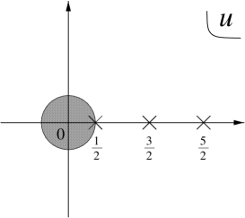
Figure 1: Analyticity of the generating function $F(r,\mu;u)$ shown on the complex $u$-plane. Poles are located at $u=\frac{1}{2},\frac{3}{2},\frac{5}{2},\cdots$. Also the domain of convergence of the series expansion at $u=0$ is shown.

Conversely from the structure of the pole of (15) nearest to $u=0$ (see Fig. 1), which limits the radius of convergence, one obtains for $n\gg 1$

$$f_{n}(r,\mu)~{}\sim~{}\frac{1}{2\pi^{2}}\,\mu\times 2^{n}.$$ (17)

Note that this asymptotic behavior is independent of $r$. This means that, although each term of the potential $V_{\beta_{0}}(r)$ is a function of $r$, its dominant part for $n\gg 1$ is only a constant potential which mimics the role of the quark mass in the determination of the quarkonium spectrum.

Thus, asymptotically, the $n$-th term of $V_{\beta_{0}}(r)$ is given by

$$V^{(n)}_{\beta_{0}}\sim-C_{F}\,4\pi\alpha_{S}(\mu)\times\frac{\mu}{2\pi^{2}}\times\biggl{\{}\frac{\beta_{0}\alpha_{S}(\mu)}{2\pi}\biggr{\}}^{n}\,\times n!.$$ (18)

As we raise $n$, first the term decreases due to powers of the small $\alpha_{S}$; for large $n$ the term increases due to the factorial $n!$. Around $n_{0}=2\pi/(\beta_{0}\alpha_{S}(\mu))$, $V^{(n)}_{\beta_{0}}$ becomes smallest. The size of the term scarcely changes within the range $n\in(n_{0}-\sqrt{n_{0}},n_{0}+\sqrt{n_{0}})$; see Fig. 2.

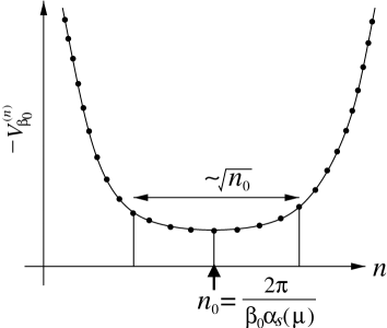
Figure 2: The graph showing schematically the asymptotic behavior of the $n$-th term of $-V_{\beta_{0}}(r)$ for $n\gg 1$.

We may consider the uncertainty of this asymptotic series as the sum of the terms within this range:

$$\delta V_{\beta_{0}}(r)\sim\sum_{n=n_{0}-\sqrt{n_{0}}}^{n_{0}+\sqrt{n_{0}}}\,\left|V^{(n)}_{\beta_{0}}\right|\sim\Lambda.$$ (19)

The $\mu$-dependence vanishes in this sum, and this leads to the claimed uncertainty.

In passing, we note that this asymptotic series is not Borel summable; a Borel summable series has terms alternating in sign, but the asymptotic series originating from the QCD infrared renormalon has terms with the same sign. We cannot circumvent the uncertainty by Borel summation of the series.

3 Renormalon Cancellation in the Total Energy of a $q\bar{q}$ system

Now we state how the problem can be circumvented. Consider the total energy of a color-singlet non-relativistic quark-antiquark pair:

$$E_{\rm tot}(r)\simeq 2m_{\rm pole}+V_{\beta_{0}}(r).$$ (20)

It was found [6] that the leading renormalon contained in the potential $V_{\beta_{0}}(r)$ gets cancelled in the total energy $E_{\rm tot}(r)$ if the pole mass $m_{\rm pole}$ is expressed in terms of the $\overline{\rm MS}$ mass. The potential and the pole mass are expressed in terms of the 1-loop running coupling $\alpha_{\rm 1L}(q)$ as

$$V_{\beta_{0}}(r)=-\int\frac{d^{3}\vec{q}}{(2\pi)^{3}}\,e^{i\vec{q}\cdot\vec{r}}\,C_{F}\frac{4\pi\alpha_{\rm 1L}(q)}{q^{2}},$$ (21)

$$m_{\rm pole}\simeq m_{\overline{\rm MS}}(\mu)+\frac{1}{2}{\hbox to18.0pt{ \hbox to-5.0pt{$\displaystyle\int$} \raise-15.0pt\hbox{$\scriptstyle{q}<\mu$} }}\frac{d^{3}\vec{q}}{(2\pi)^{3}}\,C_{F}\frac{4\pi\alpha_{\rm 1L}(q)}{q^{2}}.$$ (22)

The potential $V_{\beta_{0}}(r)$ is essentially the Fourier transform of the Coulomb gluon propagator exchanged between quark and antiquark; the difference of $m_{\rm pole}$ and $m_{\overline{\rm MS}}$ is essentially the infrared portion of the quark self-energy, see Fig. 3.

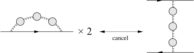
Figure 3: The 1-loop quark self-energy diagram and the one-gluon-exchange diagram between quark and antiquark, where the gluon propagators are replaced by the bubble-chains. These diagrams, respectively, contribute to the renormalons in $2m_{\rm pole}$ and $V_{\beta_{0}}(r)$.

As we saw, the renormalon uncertainty is related to the “would-be pole” contained in $\alpha_{\rm 1L}(q)$, cf. Eq. (9). The signs of the renormalon contributions are opposite between $V_{\beta_{0}}(r)$ and $m_{\rm pole}$ because the color charges are opposite between quark and antiquark while the self-enregy is proportional to the square of a same charge. Their magnitudes differ by a factor of two because both the quark and antiquark propagator poles contribute in the calculation of the potential whereas only one of the two contributes in the calculation of the self-energy. Expanding the Fourier factor in $2m_{\rm pole}$ in a Taylor series for small ${q}$,

$$e^{i\vec{q}\cdot\vec{r}}=1+{i\vec{q}\cdot\vec{r}}+\frac{1}{2}({i\vec{q}\cdot\vec{r}})^{2}+\cdots,$$ (23)

the would-be pole contained in the leading term gets cancelled against $V_{\beta_{0}}(r)$ and consequently the renormalon contributions cancel.

As a result of this cancellation, the series expansion of the total energy in $\alpha_{S}(\mu)$ behaves better if we use the $\overline{\rm MS}$ mass instead of the pole mass. Residual uncertainty due to uncancelled pole can be estimated similarly as in the previous section and is suppressed as

$$\Lambda\times\left<({\vec{q}\cdot\vec{r}})^{2}\right>\sim\Lambda\times\biggl{(}\frac{\Lambda}{\alpha_{S}m_{\rm pole}}\biggr{)}^{2},$$ (24)

which is much smaller than the original uncertainty.

4 Extracting the $\overline{\rm MS}$ masses using the Full NNLO Result

To see how well the renormalon cancellation works, we examine extractions of the bottom and top quark masses using the full next-to-next-to-leading order (NNLO) result of the boundstate spectrum. The full NNLO formula for the lowest lying ($1S$) boundstate can be calculated from the Hamiltonian Eqs. (3)-(5) and is given by [2, 7]

$$M_{1S}=2m_{\rm pole}-\frac{4}{9}\alpha_{S}(\mu)^{2}m_{\rm pole}\Biggl{[}{\textstyle\,1+\frac{\alpha_{S}(\mu)}{\pi}\biggl{\{}\Bigl{(}{\scriptstyle 11}-\frac{2}{3}n_{l}\Bigr{)}L+\Bigl{(}\frac{97}{6}-\frac{11}{9}n_{l}\Bigr{)}\biggr{\}}}~{}~{}~{}~{}~{}~{}~{}~{}~{}~{}~{}~{}~{}$$

$${\textstyle+\Bigl{(}\frac{\alpha_{S}(\mu)}{\pi}\Bigr{)}^{2}\biggl{\{}\Bigl{(}\frac{363}{4}-{\scriptstyle 11}n_{l}+\frac{1}{3}n_{l}^{2}\Bigr{)}L^{2}+\Bigl{(}\frac{927}{4}-\frac{193}{6}n_{l}+n_{l}^{2}\Bigr{)}L}~{}~{}~{}~{}~{}$$

$${\textstyle+\Bigl{(}\frac{1793}{12}+\frac{2917\pi^{2}}{216}-\frac{9\pi^{4}}{32}+\frac{275\zeta_{3}}{4}\Bigr{)}+\Bigl{(}-\frac{1693}{72}-\frac{11\pi^{2}}{18}-\frac{19\zeta_{3}}{2}\Bigr{)}n_{l}+\Bigl{(}\frac{77}{108}+\frac{\pi^{2}}{54}+\frac{2\zeta_{3}}{9}\Bigr{)}n_{l}^{2}\biggr{\}}\Biggr{]}},$$ (25)

where $L\equiv\log[\mu/(C_{F}\alpha_{S}(\mu)m_{\rm pole})]$, and $n_{l}$ denotes the number of massless quarks. We may examine the size of each term of the above perturbation series. Alternatively we may rewrite the above expression in terms of the $\overline{\rm MS}$ mass and examine the series. Presently the relation between $m_{\rm pole}$ and $\overline{m}\equiv m_{\overline{\rm MS}}(m_{\overline{\rm MS}})$ is known up to three-loop order [8]:

$$m_{\rm pole}=\overline{m}\times\biggl{[}\,1+\frac{4}{3}\Bigl{(}{\textstyle\frac{\alpha_{S}(\overline{m})}{\pi}}\Bigr{)}+\Bigl{(}{\textstyle\frac{\alpha_{S}(\overline{m})}{\pi}}\Bigr{)}^{2}(-1.0414n_{l}+13.4434)~{}~{}~{}~{}~{}~{}$$

$$+\Bigl{(}{\textstyle\frac{\alpha_{S}(\overline{m})}{\pi}}\Bigr{)}^{3}(0.6527n_{l}^{2}-26.655n_{l}+190.595)\biggr{]}.$$ (26)

First we apply the formula to the $\Upsilon(1S)$ state, for which $n_{l}=4$. Taking the input parameter as $m_{\rm pole}=4.96$ GeV/$\overline{m}=4.22$ GeV and setting $\mu=\overline{m}$ (i.e. expansion parameter is $\alpha_{S}(\overline{m})=0.22$),

$$M_{\Upsilon(1S)} = 2\times(4.96-0.05-0.08-0.11)~{}{\rm GeV}~{}~{}~{}~{}~{}\mbox{(Pole-mass scheme)}$$ (27)

$$= 2\times(4.22+0.35+0.12+0.04)~{}{\rm GeV}~{}~{}~{}~{}~{}\mbox{($\overline{\rm MS}$-scheme)}.$$ (28)

One sees that the series is not at all converging in the pole-mass scheme, whereas in the $\overline{\rm MS}$-scheme the series is converging quite nicely up to the calculated order. (See Sec. 6 for details of how we derived the series in the $\overline{\rm MS}$-scheme.) Comparing this with the experimental value $M_{\Upsilon(1S)}=9.46037\pm 0.00021$ GeV, one may extract the $\overline{\rm MS}$ bottom quark mass

$$\overline{m}_{b}\equiv m_{\overline{\rm MS}}(m_{\overline{\rm MS}})=4.22\pm 0.08~{}{\rm GeV}.$$ (29)

One might think that, looking at the behavior of the above series, we may assign a smaller theoretical uncertainty. The present uncertainty is, however, dominated by non-perturbative uncertainties other than the renormalon contributions. Thus, presently $\overline{m}_{b}$ is determined to 2% accuracy [9, 10]. It seems to be fairly good in view of the fact that its major part is controlled by perturbative QCD.

Next we turn to the (remnant of) “toponium”, for which $n_{l}=5$. At future linear $e^{+}e^{-}$ or $\mu^{+}\mu^{-}$ colliders, the top quark mass will be determined to high accuracy from the shape of the $t\bar{t}$ total production cross section in the threshold region. The location of a sharp rise of the cross section is determined mainly from the mass of the lowest lying ($1S$) $t\bar{t}$ resonance, so we will be able to measure the resonance mass and extract the top quark mass. Similarly to the previous case, we set $m_{\rm pole}=174.79$ GeV/$\overline{m}=165.00$ GeV, $\alpha_{S}(\overline{m})=0.1091$ and obtain

$$M_{1S} = 2\times(174.79-0.46-0.40-0.28)~{}{\rm GeV}~{}~{}~{}~{}~{}\mbox{(Pole-mass scheme)}$$ (30)

$$= 2\times(165.00+7.20+1.24+0.22)~{}{\rm GeV}~{}~{}~{}~{}~{}\mbox{($\overline{\rm MS}$-scheme)}.$$ (31)

In Figs. 4 are shown the convergence properties of the above series together with the corresponding cross sections.

(a)

(b)

Figure 4: The total production cross sections for $e^{+}e^{-}\to t\bar{t}$ in the threshold region, where the leading-order (LO), next-to-leading-order (NLO) and next-to-next-to-leading-order (NNLO) curves are shown. The vertical lines represent the locations of the corresponding $1S$ resonances when the top width is artificially taken to zero; also the position of $2m_{t}$ is shown by vertical lines. The two figures correspond to (a) the pole-mass scheme, and (b) the $\overline{\rm MS}$-scheme. These figures are made by T. Nagano.

In the pole-mass scheme, the convergence is very slow. According to the renormalon argument, also uncalculated higher order terms would not become much smaller. On the other hand, in the $\overline{\rm MS}$-scheme the series shows a healthy convergence behavior. For top quark, non-perturbative uncertainties are much smaller than the present perturbative theoretical uncertainty. Thus, from the above series we estimate that $\overline{m}_{t}$ can be determined to around 100 MeV accuracy [11].

5 Physical Implications

Let us discuss some physical implications of renormalon cancellation in the heavy quarkonium system. Firstly, as already mentioned, we expect that gluons with wavelength much longer than the size of the quarkonium cannot couple to this system. Hence, we expect that infrared gluons with momentum transfer $q\ll\alpha_{S}m$ should decouple from the expression of $E_{\rm tot}$. This is a naive expectation based on classical dynamics. Such understanding should be valid when it is described by the bare QCD Lagrangian without large quantum corrections. The $\overline{\rm MS}$ mass is closely related to the bare mass of quark; only ultraviolet divergences are subtracted. On the other hand, the pole mass has much more intricate relation to the bare mass, because the relation includes in addition infrared dynamics of the quantum correction to the quark self-energy. In this sense it would be natural to expect the decoupling phenomenon to be realized when the $\overline{\rm MS}$ mass is used to express $E_{\rm tot}$.

Secondly, the pole mass of a quark is ill-defined beyond perturbation theory. It can be determined only when the quark can propagate an infinite distance. Generally accepted belief is that when quark and antiquark are separated beyond a distance $\sim\Lambda^{-1}$ the color flux is spanned between the two charges due to non-perturbative effects and the free quark picture is no longer valid. On the other hand, it is natural to consider the total energy (or the mass) of a quarkonium which is a color-singlet state. It can propagate for a long time and the notion of its mass is not limited by the hadronization scale.

Thirdly, renormalon cancellation seems to be a universal feature which occurs process independently. The same phenomenon was known e.g. in the QCD corrections to the $\rho$-parameter [12] and $B$ decays [13]. Therefore, the $\overline{\rm MS}$ mass, which is determined accurately from the quarkonium spectum, would be more suited than the pole mass for an input parameter in describing other physical processes.

6 How to Cancel Renormalons in the Quarkonium Spectrum

There is one non-trivial point in realizing renormalon cancellation in the perturbation series of the quarkonium spectrum. When the pole mass and the binding energy are given as series in $\alpha_{S}$, renormalon cancellation takes place between the terms whose orders in $\alpha_{S}$ differ by one [14]:

(32)

cf. Eqs. (25) and (26). Intuitively this can be seen from the diagrams shown in Fig. 5.

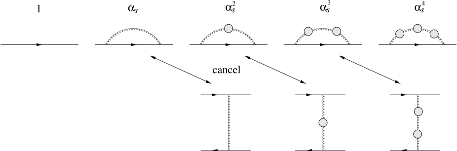
Figure 5: The figure showing how cancellations should take place between the diagrams. The orders of the potential graphs are shifted by one power of $\alpha_{S}$ which is provided by the inverse of the Bohr radius $\left<\frac{1}{r}\right>\sim\alpha_{S}m$.

An additional power of $\alpha_{S}$ in the binding energy is provided by the inverse of the Bohr radius $\left<r^{-1}\right>\sim\alpha_{S}m$,

$$\mbox{i.e.}~{}~{}~{}~{}~{}~{}~{}~{}~{}~{}~{}~{}~{}~{}\left<C_{F}\frac{\alpha_{S}^{n}}{r}\right>\sim\alpha_{S}^{n+1}m.$$ (33)

Still, one might wonder how cancellation can ever take place between different orders in $\alpha_{S}$ for any value of $\alpha_{S}$. So we demonstrate the cancellations at large orders in a specific example. The mass of the $1S$ boundstate can be written in the form of an expectation value as

$$M_{1S}=\left<{1S}\,\right|2m_{\rm pole}+\hat{H}\left|\,{1S}\,\right>$$ (34)

using the Hamiltonian (2) and its 1S energy eigenstate $\left|\,{1S}\,\right>$. We are interested in the leading renormalon contributions, so we replace

$$2m_{\rm pole}+\hat{H}~{}~{}~{}\to~{}~{}~{}2m_{\rm pole}+V_{\beta_{0}}(r).$$ (35)

The energy eigenstate can be expanded in $1/c$:

$$\left|\,{1S}\,\right>=|\,{1S}^{(0)}\rangle+\frac{1}{c}|\,{1S}^{(1)}\rangle+\frac{1}{c^{2}}|\,{1S}^{(2)}\rangle+\cdots$$ (36)

Renormalon cancellation takes place in arbitrary combination of $\langle{1S}^{(i)}|\cdots|{1S}^{(j)}\rangle$, but for simplicity we evaluate only the following part:

$$M_{1S}^{(0)}=\langle{1S}^{(0)}|\,2m_{\rm pole}+V_{\beta_{0}}(r)\,|{1S}^{(0)}\rangle=2m_{\rm pole}+\langle{1S}^{(0)}|\,V_{\beta_{0}}(r)\,|{1S}^{(0)}\rangle.$$ (37)

The second term corresponds to the binding energy and we may evaluate it at each order of the perturbation series:

$$\langle{1S}^{(0)}|V_{\beta_{0}}(r)|{1S}^{(0)}\rangle = \int_{0}^{\infty}dr\,r^{2}\,|R(r)|^{2}\,V_{\beta_{0}}(r)$$ (38)

$$= -\frac{1}{2}\,C_{F}^{2}\,\alpha_{S}(\mu)^{2}\,m_{\rm pole}\times\sum_{n=0}^{\infty}\,\biggl{\{}\frac{\beta_{0}\alpha_{S}(\mu)}{4\pi}\biggr{\}}^{n}\,g_{n}(\mu a_{0})\times n!,$$

where the zeroth-order $1S$ Coulomb wave function is given by

$$R(r)=\frac{2}{a_{0}^{3/2}}\,e^{-r/a_{0}}~{}~{},~{}~{}~{}~{}~{}~{}~{}~{}a_{0}=\biggl{(}{\textstyle\frac{1}{2}}C_{F}\alpha_{S}(\mu)m_{\rm pole}\biggr{)}^{-1}~{}:~{}\mbox{Bohr radius}.$$ (39)

$g_{n}(\mu a_{0})$’s are polynomials of $\log(\mu a_{0})$. Using the generating function method, one obtains the asymptotic form

$$g_{n}(\mu a_{0})\sim\frac{2}{\pi}\,\mu a_{0}\times 2^{n}\propto\frac{1}{\alpha_{S}}.$$ (40)

Thus, for $n\gg 1$, it becomes proportional to $\alpha_{S}^{-1}$ and effectively shifts the order of $\alpha_{S}$. By setting $\mu=\overline{m}$, it is easy to check that in this example the leading renormalon cancels as in Eq. (32) and the residual piece behaves as

$$\Bigl{[}\mbox{$n$-th term of}~{}M_{1S}^{(0)}\Bigr{]}\sim\alpha_{S}(\overline{m})\,\overline{m}\times n!\times\biggl{\{}\frac{\beta_{0}\alpha_{S}(\overline{m})}{6\pi}\biggr{\}}^{n}.$$ (41)

It follows that

$$\delta M_{1S}^{(0)}\sim\Lambda\times\biggl{(}\frac{\Lambda}{\alpha_{S}\overline{m}}\biggr{)}^{2}\ll\Lambda.$$ (42)

From this example one learns that the cancellation of renormalon contribution between shifted orders $A_{n}\,\alpha_{S}^{n}$ and $B_{n+1}\,\alpha_{S}^{n+1}$ should be properly taken into account when expressing the boundstate mass as a perturbation series. There are many different prescriptions to accomplish this. We derived the series (28) and (31) in the following manner. We have rewritten Eq. (25) as

$$M_{1S} = 2m_{\rm pole}\times\biggl{[}\,1+\sum_{n=2}^{4}\,P_{n}\,\alpha_{S}(\overline{m})^{n}\biggr{]}$$ (43)

$$= 2\overline{m}\times\biggl{[}\,1+\sum_{n=1}^{3}\,A_{n}\,\alpha_{S}(\overline{m})^{n}\biggr{]}\times\biggl{[}\,1+\sum_{n=2}^{4}\,P_{n}\,\alpha_{S}(\overline{m})^{n}\biggr{]},$$

where $P_{n}$’s are polynomials of $\log\Bigl{(}\alpha_{S}(\overline{m})\Bigr{)}$ and $A_{n}$’s are just constants independent of $\alpha_{S}(\overline{m})$. We identified $P_{n}\alpha_{S}^{n}$ as order $\alpha_{S}^{n-1}$ and then reduced the last line to a single series in $\alpha_{S}$.

Parametric accuracy of the last terms of Eqs. (28) and (31) is $\alpha_{S}^{3}\overline{m}$. In order to improve the accuracy to $\alpha_{S}^{4}\overline{m}$, we need to know further (a) the exact 4-loop relation between $m_{\rm pole}$ and $\overline{m}$, and (b) the binding energy at order $\alpha_{S}^{5}$ in the large-$\beta_{0}$ approximation.

7 Some Questions

One can ask some interesting questions related to the renormalon problem and extraction of quark mass. In the case of top quark, its mass will also be measured from the invariant mass distribution of decay products of the top quark in future hadron collider experiments and in future $e^{+}e^{-}$ collider experiments. What is the mass extracted from the peak position of the Breit-Wigner distribution? Naively it is the pole mass because the peak position is determined from the position of the pole of the top quark propagator in perturbative QCD. On the other hand, as we have seen, the pole mass suffers from a theoretical uncertainty of ${\cal O}$(300 MeV). Since future experiments will be able to determine the peak position of the invariant mass distribution to ${\cal O}$(100 MeV) accuracy, we will indeed face this serious conceptual problem. We believe that renormalon cancellation also takes place in this physical quantity. But the problem lies in the fact that we have no reliable theoretical method to calculate the invariant mass distribution of realistic color-singlet final states. Rather we calculate the invariant mass of final partons which do not combine to color-singlet state. Another question is whether the peak position of invariant mass distribution measured in hadron collider experiments will be the same as that measured in $e^{+}e^{-}$ collider experiments. The answer is probably no, since at hadron colliders top and antitop are pair-created not necessarily in a color-singlet state.

These are very interesting questions which are worth further studies.

References

• [1] M. Beneke, Phys. Rept. 317, 1 (1999).
• [2] A. Pineda and F. Ynduráin, Phys. Rev. D58, 094022 (1998).
• [3] A. Hoang and T. Teubner, Phys. Rev. D58, 114023 (1998); K. Melnikov and A. Yelkhovsky, Nucl. Phys. B528, 59 (1998).
• [4] M. Beneke and V. Braun, Nucl. Phys. B426, 301 (1994); I. Bigi, et al., Phys. Rev. D50, 2234 (1994).
• [5] U. Aglietti and Z. Ligeti, Phys. Lett. B364, 75 (1995).
• [6] A. Hoang, M. Smith, T. Stelzer and S. Willenbrock, Phys. Rev. D59, 114014 (1999); M. Beneke, Phys. Lett. B434, 115 (1998).
• [7] K. Melnikov and A. Yelkhovsky, Phys. Rev. D59, 114009 (1999).
• [8] K. Chetyrkin and M. Steinhauser, Phys. Rev. Lett. 83, 4001 (1999); hep-ph/9911434; K. Melnikov and T. v. Ritbergen, hep-ph/9912391.
• [9] A. Hoang, Phys. Rev. D61, 034005 (2000); M. Beneke and A. Signer, Phys. Lett. B471 233, (1999).
• [10] M. Beneke, hep-ph/9911490.
• [11] A. Hoang, et al., hep-ph/0001286.
• [12] P. Gambino and A. Sirlin, Phys.Lett. B355, 295 (1995).
• [13] M. Beneke, V. Braun and V. Zakharov, Phys. Rev. Lett. 73, 3058 (1994); M. Luke, A. Manohar and M. Savage, Phys. Rev. D51 4924 (1995); M. Neubert and C. Sachrajda, Nucl. Phys. B438, 235 (1995).
• [14] A. Hoang, Z. Ligeti and A. Manohar, Phys. Rev. Lett. 82, 277 (1999); Phys. Rev. D59, 074017 (1999).