Present Status of the Long Range Component of the Nuclear Force

Abstract

In order to settle the fundamental question whether the nuclear forces involve the long range components, the S-wave amplitude of the proton-proton scattering is analysed in search for the extra singularity at $\nu=0$, which corresponds to the long range force. To facilitate the search, a function, which is free from the singularities in the neighborhood of $\nu=0$ when all the interactions are short range, is constructed. The calculation of such a function from the phase shift data reveals a sharp cusp at $\nu=0$ in contradiction to the meson theory of the nuclear force. The type of the extra singularity at $\nu=0$ is close to what is expected in the case of the strong van der Waals interaction. Physical meanings of the long range force in the nuclear force are discussed. Low energy p-p experiments to confirm directly the strong long range interaction are also proposed, in which the characteristic interference patten of the Coulonb and the Van der Waals forces is predicted.

1 Introduction

In the Yukawa model of the nuclear force[1], the pi-meson plays the central roll, since the nuclear potentials are assumed to arise from the exchanges of a pion and a set of pions at least outside of the inner core region. Although the two-pion exchange potentials constructed directly from the meson theory are not successful in understanding the details of the data of the nucleon-nucleon scatterings, various phenomenological nuclear potentials have been proposed to reproduce the existing data. In the constructions of the nuclear potentials, two features are commonly shared by all the nuclear potentials, which are inherited from the meson theory of the nuclear force. One is the one-pion exchange (OPE) part of the potential and the other is that the range of the non-OPE part is shorter than $1/(2\mu)$. In terms of the singularities of the scattering amplitudes $A(s,t)$, such features correspond to the one-pion exchange pole at $t=\mu^{2}$ and the cut of the two-pion exchange which starts at $t=4\mu^{2}$. These analytic structures are common to all the amplitudes calculated from the various proposed nuclear potentials.

On the other hand, in the nineteen sixties our views on the nucleons changed from ‘elementary particles’ to composite particles, and moreover in the most important models of hadron, such as the QCD and the dyon model[2], the constructive forces of the composite particles are the Coulombic types. Therefore we cannot exclude the possibility for the induced long range force to appear between the composite particles. In particular, in the dyon model of hadron, the appearance of the strong van der Waals interaction between hadrons is a natural cosequence, because in such a model the hadrons are regarded as the ‘magnetic atoms’[3]. In general the long range force gives rise to a singularity at $t=0$ in the scattering amplitude $A(s,t)$, and therefore the analytic structure is completely different from the case of the purely short range interactions.

Since there is no apriori reason to believe that the strong  interaction is a synonym for the short range interaction, it is desirable to search for the possible long range components of the nuclear force, whenever new precise data in $|t|\ll 4\mu^{2}$ come to be available. It is the difference of the analytic structure that allows us to do the search in the clear-cut way without being disturbed by the ambiguities such as different parametrization of the nuclear potentials in the inner region. Therefore, our aim in the present article is to search for the possible extra singularity of $A(s,t)$ at $t=0$, which is characteristic of the long range force, or to find the corresponding extra singularity in the partial wave amplitude. It is important that the search of the extra singularity can be carried out independently of the uncertainties of the spectra related to other singularities. The reason of such possibility comes from the fact that the location of the extra singularity is the end point of the physical region $-4\nu\leq t\leq 0$, where the experimental data are available. Therefore, in contrast to the search for the short range force, our search of the extra singularity at $t=0$ does not require any analytic continuation from the physical region. In our approach based on the analytic structure, the dispersion technique will turn out to be useful.

In the search of the long range force, the required accuracy of the input data depends heavily on the power $\gamma$ of the threshold behavior of the spectral function $A_{t}(s,t)$ at $t=0$, where for small $\nu$ and $|t|$ the power $\gamma$ is introduced by $A_{t}(s,t)=\pi C^{\prime}t^{\gamma}+\cdots$. Since $\gamma$ and another power $\alpha$, which appears in the asymptotic behavior of the long range potential as $V(r)\sim-C/r^{\alpha}$, are related by $\alpha=2\gamma+3$, our observation of the extra singularity in the amplitude becomes more and more difficult and requires the higher precision of the input data, as $\alpha$ increases. For example, the van der Waals potentials of the London type ($\alpha=6$) and the Casimir-Polder type ($\alpha=7$) imply $\gamma=1.5$ and $\gamma=2.0$ respectively, and therefore to observe these van der Waals forces is to recognize the singularities of the type $C^{\prime}(-t)^{3/2}$ or $C^{\prime}t^{2}\log(-t)$ on the smooth back ground function of $A(s,t)$. In order to observe the long range force, it is essential to obtain the high precision data at least in the region of small $|t|$, when the power $\alpha$ of the asymptotic potential is not small.

In the hadron physics, the accuracies of the phase shift data of the S-wave proton-proton scattering in the low energy region are exceptinally high[4], and so it is better to analyse the S-wave amplitude $h_{0}(\nu)$ instead of $A(s,t)$ in our search for the long range force. After the partial wave projection, the singularity of $A(s,t)$ at $t=t_{1}$ becomes the left hand singularity at $\nu=-t_{1}/4$ in $h_{0}(\nu)$. Therefore the extra singularity at $t=0$ appears at $\nu=0$, whereas the OPE pole changes to the logarithmic cut starting at $\nu=-\mu^{2}/4$, and the two-pion exchange spectrum starts at $\nu=-\mu^{2}$ in $h_{0}(\nu)$. In addition to these singularities, $h_{0}(\nu)$ has the unitarity cut in $\nu\geq 0$. Moreover since we are considering the proton-proton scattering, $h_{0}(\nu)$ has also the cuts of the Coulombic interaction in $-\infty<\nu\leq 0$ and of the vacuum polarization in $-\infty<\nu\leq-m_{e}^{2}$ .

In section 2, we shall construct a function $K_{0}(\nu)$ whose non-OPE part is free from the singularities in $|\nu|<\mu^{2}$, when the forces are the short range types of the meson theory plus the electromagnetic interaction. If we take advantage that the scattering length is known within $0.05\%$, we can even consider the once subtracted function $K_{0}^{once}(\nu)=(K_{0}(\nu)-K_{0}(0))/\nu$. The merit to use the once subtracted function instead of $K_{0}(\nu)$ is that, since the power of the threshold behavior at $\nu=0$ changes from $\gamma$ to $(\gamma-1)$, the extra singularity becomes much easier to be obsreved, when it exists. In section 3, by using the phase shift data we shall evaluate numerically the once subtracted Kantor amplitude $K^{once}_{0}(\nu)$, and its non-OPE part $\tilde{K}^{once}_{0}(\nu)$ will be tabulated. The result of the evaluation is that $\tilde{K}_{0}^{once}(\nu)$ has a sharp cusp at $\nu=0$.

In sections 4 and 5, $\tilde{K}_{0}^{once}(\nu)$ is fitted by using the spectrum of the long range force and that of the short range force respectively. It turns out in section 4 that the chi-square minimum occurs at $\gamma=1.48\sim 1.62$, which is close to the $\gamma$ of the van der Waals interaction of the London type. In section 5, it is shown that the conventional spectrum of the short range interaction cannot reproduce the cusp.

In section 6, by assuming that the well-known mechanism to produce the van der Waals force is working, the lower bound of the strength ${}^{\ast}e^{2}$ of the underlying Coulombic force is estimated by using the inequality of the strength $C_{6}$ of the Van der Waals potential. The lower bound of ${}^{\ast}e^{2}$ becomes 3.3 or 14 depending on the value of the radius of the composite particle, which comes from the measurement of the nucleon form factor or the distance where the deviation from the asymptotic form of the van der Waals potential becomes appreciable, respectively. In section 6, it is also pointed out that the Coulombic interaction between the magnetic monopoles is an imprtant candidate of the underlying super-strong Coulombic force, and the dyon model of hadron is explained briefly. Section 7 is used for remarks and comments, in which low energy experiments to confirm the long range force, by observing the characteristic destructive interference pattern of the Coulomb and the strong Van der Waals forces, are proposed .

2 Selection of a Regular Function

The low energy proton-proton scattering is prominent in its accuracy of the measurements in the hadron physics. Especially the S-wave amplitude $h_{0}(\nu)$ in the low energy region provides the ideal place to answer to the fundamental question whether the hadron-hadron interactions are short range except for the electromagnetic components. In the following investigations, we shall make use of the difference of the analytic structures of the amplitudes $h_{0}(\nu)$. In general, for the short range interaction which arises from the exchange of a state with mass $\sqrt{t_{1}}$, a singularity appears at $\nu=-t_{1}/4$ in the partial wave amplitude $h_{0}(\nu)$. On the other hand, the long range interaction gives rise to a singularity at $\nu=0$. Since the location of the extra singularity due to the long range force is the end point of the physical region $\nu\geq 0$, where the experimental data are available, we can expect to observe the singularity directly, if it exists, without making any analytic continuation from the physical region. The first thing we have to do is to construct a function which is regular at $\nu=0$, when all the interactions are short range. Next thing is to eliminate the known near-by singularities from the function. The function with such a wider domain of analyticity serves to expose the extra singularity at $\nu=0$, and makes it easier for us to observe the long range interaction, when it exists.

Although the main aim of this section is to construct such an analytic function for the proton-proton scattering where the effects of the vaccum polarization as well as the Coulomb interaction are not negligible, it is instructive to start by constructing such a function for the neutron-neutron scattering first. It is well-known that the S-wave amplitude $h_{0}(\nu)$ has the unitarity cut in $\nu>0$ with the spectral function Im$h_{0}(\nu)$, where $h_{0}(\nu)$ relates to the phase shift by

$$h_{0}(\nu)=\frac{\sqrt{m^{2}+\nu}}{\sqrt{\nu}}e^{i\delta_{0}(\nu)}\sin\delta_{0}(\nu)\quad.$$ (1)

The most famous function, which is analytic at $\nu=0$ and therefore accepts the Taylor expansion of $\nu$ when all forces are short range, is the effective range function $X_{0}(\nu)$ of Bethe. As it is well-known, $X_{0}(\nu)$ is defined by

$$X_{0}(\nu)=\sqrt{\nu}\cot\delta_{0}(\nu).$$ (2)

From Eqs.(1) and (2), the relation between $h_{0}(\nu)$ and $X_{0}(\nu)$ is

$$h_{0}(\nu)=\frac{\sqrt{m^{2}+\nu}}{X_{0}(\nu)-i\sqrt{\nu}}\quad.$$ (3)

Since the one-pion exchange (OPE) contribution is

$$h_{0}^{1\pi}(\nu)=\frac{1}{4}\frac{g^{2}}{4\pi}\frac{\mu^{2}}{4\nu}\log(1+\frac{4\nu}{\mu^{2}})\quad,$$ (4)

the values of the coupling constant $g^{2}/4\pi$ and the neutral pion mass $\mu$ are sufficient to eliminate the OPE cut from $h_{0}(\nu)$. In fact $\tilde{h}_{0}(\nu)\equiv h_{0}(\nu)-h_{0}^{1\pi}(\nu)$ does not have the OPE cut. However Eq.(3) indicates that in order to eliminate the OPE cut from $X_{0}(\nu)$ information on Re$\,h_{0}(\nu)$ in $\nu\leq-\mu^{2}/4$ as well as $g^{2}/4\pi$ and $\mu$ are necessary. Therefore the effective range function $X_{0}(\nu)$ is not adequate for our purpose to construct a function with wider domain of analyticity.

Another possibility is the Kantor amplitude[5], which is defined by

$$K_{0}(\nu)=h_{0}(\nu)-\frac{1}{\pi}\int_{0}^{\infty}d\nu^{\prime}\frac{{\rm Im}\;h_{0}(\nu^{\prime})}{\nu^{\prime}-\nu}\quad.$$ (5)

The Kantor amplitude does not have the unitarity cut, and the values of $K_{0}(\nu)$ for real positive $\nu$ can be evaluated directly from the experimental data, although the integration must be regarded as the principal value integration of Cauchy. It is straightforward to eliminate the OPE cut from the Kantor amplitude, and which is achieved by introducing the non-OPE Kantor amplitude $\tilde{K}_{0}(\nu)$ by

$$\tilde{K}_{0}(\nu)=K_{0}(\nu)-K_{0}^{1\pi}(\nu)\quad,$$ (6)

where the OPE part of the Kantor amplitude is common to that of the partial wave amplitude, namely $K_{0}^{1\pi}(\nu)=h_{0}^{1\pi}(\nu)$. It is useful to rewrite the Kantor amplitude introduced in Eq.(5) into the form of the contour integration,

$$K_{0}(\nu)=-\frac{1}{2\pi i}\int_{C}d\nu^{\prime}\frac{h_{0}(\nu^{\prime})}{\nu^{\prime}-\nu}\quad,$$ (7)

where the closed contour $C$ is shown in Figure 1. The merit to write $K_{0}(\nu)$ in the form of Eq.(7) is that because of Eq.(3), when the effective range function $X_{0}(\nu)$ is a polynomial of $\nu$ or more generally a meromorphic function of $\sqrt{\nu}$, then the only singularities of $h_{0}(\nu)$ on the first sheet of $\nu$ are poles. Therefore by shrinking the contour $C$ to a point, $K_{0}(\nu)$ becomes the sum of the contributions of the poles on the first sheet of $\nu$ or in the upper half $\sqrt{\nu}$-plane. In this way, we need not carry out the principal value integration of the rapidly changing function of Eq.(5). This technique to change the integration into the sum of the contributions of poles will be used in the actual calculation of $K_{0}(\nu)$ in the next section. We are now in the position to examine $\tilde{K}_{0}(\nu)$ in search for the extra singularity at $\nu=0$, if the precise data of the neutron-neutron scatterings were available.

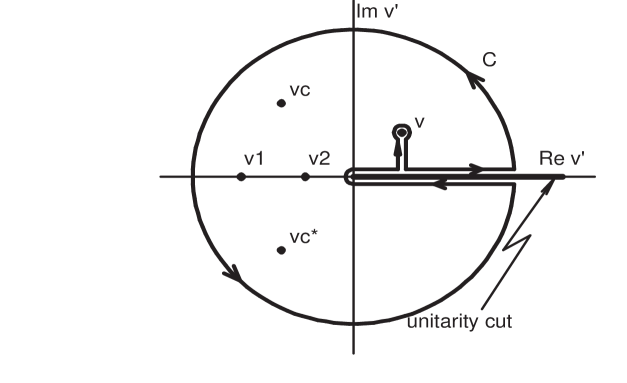
Figure 1: The contour $C$ of the integration in Eq.(7). $\nu_{1}$ and $\nu_{2}$ are real poles on negative real axis, whereas $\nu_{c}$ and $\nu_{c}^{\ast}$ are a pair of complex poles on the $\nu^{\prime}$-plane. Their values are listed in Table 2.

Let us turn to the proton-proton scattering, where the vacuum polarization as well as the Coulombic interactions are important. The Kantor amplitude introduced in Eq.(5) does not satisfy our requirement of the analyticity. This is because the Coulombic cut in $-\infty<\nu\leq 0$ and the cut of the vaccum polarization in $-\infty<\nu\leq-m_{e}^{2}$ still remain in the Kantor amplitude $K_{0}(\nu)$ of Eq.(5). The difficulties are by-passed if we remember the modified effective range function $X_{0}(\nu)$ of the proton-proton scattering, which is regular at $\nu=0$ and accepts the effective range expansion, when all the forces are short range except for the terms of the Coulomb and of the vacuum polarization. The modified effective range function $X_{0}(\nu)$ for the phase shift $\delta_{0}^{E}(\nu)$ is

$$X_{0}(\nu)=\frac{C_{0}^{2}\sqrt{\nu}}{1-\phi_{0}}\{(1+\chi_{0})\cot\delta_{0}^{E}-\tan\tau_{0}\}+me^{2}h(\eta)+me^{2}\ell_{0}(\eta)\quad.$$ (8)

In Eq.(8), two well-known functions with the Coulombic order of magnitudes appear, they are expressed using a new variable $\eta=me^{2}/(2\sqrt{\nu})$ :

$$C_{0}^{2}=\frac{2\pi\eta}{e^{2\pi\eta}-1}\qquad\;and\qquad\;h(\eta)=\eta^{2}\sum_{\ell=1}^{\infty}\frac{1}{\ell(\ell^{2}+\eta^{2})}-\log\eta-0.57722\cdots.$$ (9)

In Eq.(7) $\tau_{0}$ is the phase shift due to the vacuum polarization potential[6]

$$V^{vac}(r)=\lambda\frac{e^{2}}{r}\int_{4m_{e}^{2}}^{\infty}dt\frac{e^{-r\sqrt{t}}}{2t}(1+\frac{2m_{e}^{2}}{t})\sqrt{1-\frac{4m_{e}^{2}}{t}}\equiv\lambda\frac{e^{2}}{r}I(r)\quad,$$ (10)

where $m_{e}$ is the mass of the electron and $\lambda=2e^{2}/3\pi=1.549\times 10^{-3}$. Functions $\tau_{0}$, $\chi_{0}$, $\phi_{0}$ and $\ell_{0}(\eta)$ have the order of magnitudes of the vaccum polarization, and it is sufficient for our purpose to retain only the first term in $\lambda$. In such approximation, they are expressed by $F_{0}(r)$ and $G_{0}(r)$, which are the regular and the irregular Coulombic wave functions respectively, as

$$\tau_{0}=-2\eta\lambda\int^{\infty}_{0}dr\frac{F_{0}(r)^{2}I(r)}{r}\\$$ (11)

$$\chi_{0}=\phi_{0}=-2\eta\lambda\int_{0}^{\infty}dr\frac{F_{0}(r)G_{0}(r)I(r)}{r}\\$$ (12)

$$\ell_{0}(\eta)=-\lambda\int_{0}^{\infty}dr\frac{I(r)}{r}[(CG_{0}(r))^{2}-(CG_{0}(r))^{2}_{\nu=0}]\quad,$$ (13)

where $I(r)$ is defined in Eq.(10). Exact definitions of these functions are found in the paper by Heller[6].

By using the modified effective range function $X_{0}(\nu)$, we define the S-wave amplitude $h_{0}(\nu)$ of the p-p scattering by

$$h_{0}(\nu)=\frac{\sqrt{m^{2}+\nu}}{X_{0}(\nu)-me^{2}h(\eta)-i\sqrt{\nu}C_{0}^{2}}\quad.$$ (14)

The relation between $h_{0}(\nu)$ and the phase shift $\delta_{0}^{E}$ is obtained if we substitute $X_{0}(\nu)$ of Eq.(8) into Eq.(14), and which reduces to the well-known form

$$h_{0}(\nu)=\frac{1}{C_{0}^{2}}\frac{\sqrt{m^{2}+\nu}}{\sqrt{\nu}}e^{i\delta_{0}^{E}(\nu)}\sin\delta_{0}^{E}(\nu)\quad,$$ (15)

if the functions related to the vacuum polarization are neglected. The form of $h_{0}(\nu)$ of Eq.(15) is the same as that of the neutron-neutron scattering of Eq.(1) except for the factor $C_{0}^{2}$ given in Eq.(9), which is the penetration factor. If we compare the S-wave amplitude of the p-p scattering with that of the n-n scattering, which are given in Eq.(14) and Eq.(3) respectively, a combination of functions $(-me^{2}h(\eta)-i\sqrt{\nu}C_{0}^{2})$ appears in place of $\ -i\sqrt{\nu}$. In order to investigate the analytic structure of $h_{0}(\nu)$, it is convenient to rewrite the combination as

$$-me^{2}h(\eta)-i\sqrt{\nu}C_{0}^{2}=-i\sqrt{\nu}+me^{2}\{\log(i\eta)-\psi(1+i\eta)\}\quad.$$ (16)

Since the digamma function $\psi(z)$ has poles at non-positive integers, the poles on the $\eta$-plane appear on the positive imaginary axis. In terms of $\sqrt{\nu}$, which is $me^{2}/(2\eta)$, the series of poles appear on the negative imaginary axisis and converge to $\sqrt{\nu}=0$. It is the smallness of the fine structure constant $e^{2}$ and therefore of the residues of such poles that zeros of the denominator of Eq.(14) occur at points very close to the locations of the poles of $(-me^{2}h(\eta)-i\sqrt{\nu}C_{0}^{2})$. Therefore the partial wave amplitude $h_{0}(\nu)$ of the p-p scattering has a series of poles on the second sheet of $\nu$, namely on the lower half plane of $\sqrt{\nu}$, whereas on the first sheet of $\nu$ the analytic structure of $h_{0}(\nu)$ does not change compared to the case of the n-n scattering. This fact implies that the same definition of the Kantor amplitude $K_{0}(\nu)$ introduced for the neutron-neutron scattering, which is given in Eq.(5), is valid also for the proton-proton scattering, as long as we evaluate Im$h_{0}(\nu^{\prime})$ of Eq.(5) from Eqs.(14) and (16). Therefore the Kantor amplitude of the p-p scattering $K_{0}(\nu)$ constructed in this way is free from the singularities in the neighborhood of $\nu=0$, and so does not have the cut of the vacuum polarization as well as that of the Coulomb interaction.

3 Numerical Calculation of the Kantor
Amplitude

Since the scattering length of the S-wave amplitude of the p-p scattering is known with high precision, we shall analyse the once subtracted Kantor amplitude, which is

$$K_{0}^{once}(\nu)\equiv\frac{K_{0}(\nu)-K_{0}(0)}{\nu}.$$ (17)

Merits to use the once subtracted Kantor amplitude rather than $K_{0}(\nu)$ are twofold. The first one is the higher convergence of the integration

$$K_{0}^{once}(\nu)=\frac{h_{0}(\nu)-h_{0}(0)}{\nu}-\frac{1}{\pi}\int_{0}^{\infty}d\nu^{\prime}\frac{Im\;h_{0}(\nu^{\prime})}{\nu^{\prime}(\nu^{\prime}-\nu)}\quad,$$ (18)

namely the uncertainty arising from the lack of the very accurate data in the higher energy region is largely suppressed because of the extra factor $\nu^{\prime}$ in the denominator of the integrand. The second one is the change of the power of the threshold behavior of the spectral function from $C^{\prime}(-\nu^{\prime})^{\gamma}$ to $-C^{\prime}(-\nu^{\prime})^{\gamma-1}$, and which makes it easier for us to recognize the extra singularity at $\nu=0$ in $K_{0}^{once}(\nu)$. Since the power $\alpha$, which appears in the asymptotic behavior of the potential as $V(r)\sim-C_{\alpha}/r^{\alpha}$, and the power $\gamma$ of the spectral function Im$\>h_{0}(\nu^{\prime})$ are related by

$$\alpha=2\gamma+3\quad,$$ (19)

$\gamma$ is equal to $3/2$ for the van der Waals potential of the London type, and which is expected to occur in the dyon model of hadron[2][3]. Therefore in such a case the behavior of the once subtracted Kantor amplitude in the neighborhood of $\nu=0$ is that

$$K_{0}^{once}(\nu)={\rm const.}+C^{\prime}\sqrt{\nu}+\cdots\qquad{\rm with}\quad C^{\prime}>0\quad,$$ (20)

and we must observe the extra singularity as a cusp at $\nu=0$ unless the coefficient $C^{\prime}$ is very small.

Let us represent the effective range function of the p-p scattering $X_{0}(\nu)$ by a meromorphic function of $\nu$:

$$\frac{X_{0}(\nu)-c_{0}-c_{1}\nu}{\nu}(1-\frac{\nu}{\nu_{P}})=a_{0}+a_{1}\nu+\frac{b_{0}+b_{1}\nu}{d_{0}+d_{1}\nu+\nu^{2}}\quad,$$ (21)

in which $\nu_{P}$ is the location of the pole of $X_{0}(\nu)$. $-c_{0}$ and $c_{1}$ are the inverse of the scattering length and the effective range devided by 2 respectively. The r.h.s. of Eq.(21) involves six free parameters to be fitted. In the fitting, the Compton wave length of the neutral pion will be used as the unit of the length. In the search of the free parameters, $c_{0}$, $c_{1}$ and $\nu_{P}$ are fixed beforehand which are[7]

$$c_{0}=0.18698\quad,\quad c_{1}=0.9541\quad and\quad\nu_{P}=6.39\qquad.$$ (22)

Accuracies of $c_{0}$ and $c_{1}$ are as high as 0.05% and 0.6% respectively. On the other hand, uncertainty of $\nu_{P}$ is around 3 per cent. However reasonable accuracy of $\nu_{P}$ is sufficient for our purpose to search for the extra singularity at $\nu=0$ .

The S-wave phase shifts of the p-p scattering by the Nijmegen group[7][8][9] are used as the input to evaluate the effective range function $X_{0}(\nu)$. The once subtracted form of $X_{0}(\nu)$, in which the pole at $\nu=\nu_{P}$ is eliminated by multiplying a factor $(1-\nu/\nu_{P})$, is displayed in figure 2. The points in the figure come from the multi-energy phase shifts of Nijmegen-90 [8].

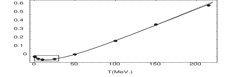
Figure 2: $(X_{0}(\nu)-c_{0}-c_{1}\nu)(1-\nu/\nu_{P})/\nu$ of Eq.(21) is plotted against $T_{lab}$, where $X_{0}(\nu)$ is the effective range function of the S-wave p-p scattering. The points are the data of Nijmegen 90. The box of the left lower corner is enlarged in fig.3.

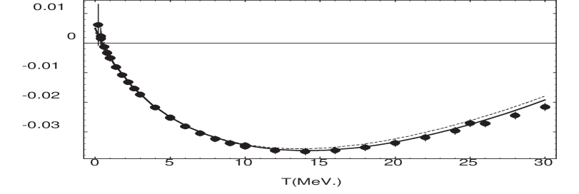
Figure 3: Enlarged graph of $(X_{0}(\nu)-c_{0}-c_{1}\nu)(1-\nu/\nu_{P})/\nu$ with error bar is plotted against $T_{lab}$ in $T_{lab}\leq 30\;MeV.$, in which the points are the data of Nijmegen 88 and 90. The parameters of the fitted curves are listed in Table 1.

The box at the left lower corner in the figure is enlarged and displayed in figure 3, and in which the low energy data in the energy range $0.1\;MeV.\leq T_{lab}\leq 30\;MeV.$ of Nijmegen-88 [7] are shown with their error bars. The data in $0.5\;MeV.\leq T_{lab}\leq 100\;MeV.$ are fitted by the meromorphic function of Eq.(21), and the six parameters are determined by the chi square search. The searched curve is shown in figures 2 and 3 as the full line, and whose parameters are tabulated in the column [sc] in Table 1. On the other hand the dash curve in the figures is a different fit by a meromorphic function, in which the six parameters are fixed by the six data points at $T_{lab}=$ 1, 5, 10, 25, 50, 100 MeV. of the Nijmegen-90[8]. The parameters of the fixed curve are tabulated in the column [fc] in Table 1.

Table 1: Parameters of the meromorphic form of the effective range function introduced in Eq.(21)

	[uc]	[sc]	[$l$c]	[fc]
$a_{0}$	$-$0.2579	$-$0.2703	$-$0.2815	$-$0.3295
$a_{1}$	0.15278	0.15504	0.15694	0.16328
$b_{0}$	0.01009	0.01983	0.03463	0.09272
$b_{1}$	0.1862	0.2098	0.2337	0.39475
$d_{0}$	0.0379	0.0720	0.1218	0.2782
$d_{1}$	0.812	0.927	1.061	1.643

In the same table, there are also columns of the curves of [$l$c] and [uc], in which the parameters are determined by fitting to the lower fringe and to the upper fringe of the error bars in $0.5MeV.\leq T_{lab}\leq 100\;MeV.$ respectively. Such parameters are necessary to estimate the errors of the Kantor amplitude.

It is remarkable that in figures 2 and 3, the curvature of the curve in the small $T_{lab}$ region increases very rapidly as $T_{lab}$ decreases to zero. If we remember that the starting points of the spectra of the one-pion exchange(OPE) and of the two-pion exchange(TPE) are $T_{lab}=-9.71\;MeV.$ and $-38.83\;MeV.$ repectively, it is not easy to understand the rapid change of the curvature in the low energy region such as $0<T_{lab}<10\;MeV.$ . On the other hand, if we accept the long range force, the appearance of such a cusp at $T_{lab}=0$ is what is expected. Since the separation of the OPE term from $X_{0}(\nu)$ is not simple, in the present article we shall examine $K_{0}^{once}(\nu)$ because, contrary to $X_{0}(\nu)$, the separation of the OPE term from the Kantor amplitude is straightforward.

Table 2: Poles and residues of $h_{0}(\nu)$ for meromorphic $X_{0}(\nu)$

	[uc]	[sc]	[$l$c]	[fc]
$\nu_{1}$	$-$0.04951	$-$0.08487	$-$0.12894	$-$0.18430
$r_{1}$	0.005345	0.016313	0.044157	0.15756
$\nu_{2}$	$-$0.54699	$-$0.58917	$-$0.63853	$-$0.87572
$r_{2}$	2.5629	2.8719	3.1755	5.0604
Re$\;\nu_{c}$	$-$3.4550	$-$2.8526	$-$2.4303	$-$1.3318
Im$\;\nu_{c}$	$-$6.0285	$-$6.0191	$-$5.9984	$-$6.0552
Re$\;r_{c}$	$-$25.427	$-$22.461	$-$20.562	$-$16.855
Im$\;r_{c}$	43.256	36.108	31.607	21.008

In Table 2, the locations of the poles of $h_{0}(\nu)$, which is introduced in Eq.(14), on the first sheet of $\nu$ and their residues are tabulated. The columns correspond to those in Table 1, and each of them has two real poles $\nu_{1}$ and $\nu_{2}$, and a pair of complex poles $(\nu_{c},\nu_{c}^{\ast})$ respectively, on the first sheet of $\nu$.

In Table 3, $\tilde{K}_{0}^{once}(\nu)$, which are the once subtracted Kantor amplitude of Eq.(17) minus the one-pion exchange contribution, are tabulated for [sc] and [fc]. Because of Eq.(7),

$$\tilde{K}_{0}^{once}(\nu)=\frac{r_{1}}{\nu_{1}(\nu-\nu_{1})}+\frac{r_{2}}{\nu_{2}(\nu-\nu_{2})}+2Re\{\frac{r_{c}}{\nu_{c}(\nu-\nu_{c})}\}+\Delta_{0}-(OPEC)$$ (23)

, where OPEC is the one-pion exchange contribution. The correction term $\Delta_{0}$ arises from the approximation to $X_{0}(\nu)$ by the meromorphic function fitted to the phase shift in the energy range of $0.5\;MeV.<T_{lab}<100\;MeV.$.

Table 3: Non-OPE part of the once subtracted Kantor amplitude $\tilde{K}_{0}^{once}(\nu)$

$\sqrt{\nu}$	$T_{lab}$	$\tilde{K}_{0}^{once}(\nu)$			$\sqrt{\nu}$	$T_{lab}$	$\tilde{K}_{0}^{once}(\nu)$
$(\mu\!=\!1)$	(MeV.)	[$\,sc\,$]	[$\,f\,c\,$]	$\Delta\tilde{K}_{0}^{once}$	$(\mu\!=\!1)$	(MeV.)	[$\,sc\,$]	[$\,f\,c\,$]	$\Delta\tilde{K}_{0}^{once}$
0.05	0.097	-5.188	-4.974	0.2803	1.15	51.35	-2.651	-2.655	0.0126
0.10	0.388	-5.049	-4.892	0.2069	1.20	55.92	-2.581	-2.584	0.0116
0.15	0.874	-4.864	-4.771	0.1307	1.25	60.67	-2.515	-2.517	0.0105
0.20	1.553	-4.671	-4.629	0.0747	1.30	65.62	-2.451	-2.453	0.0095
0.25	2.427	-4.493	-4.479	0.0418	1.35	70.77	-2.390	-2.391	0.0086
0.30	3.495	-4.335	-4.332	0.0257	1.40	76.11	-2.331	-2.332	0.0078
0.35	4.757	-4.196	-4.194	0.0193	1.45	81.64	-2.273	-2.274	0.0071
0.40	6.213	-4.070	-4.064	0.0175	1.50	87.37	-2.218	-2.218	0.0065
0.45	7.863	-3.953	-3.943	0.0174	1.55	93.29	-2.163	-2.164	0.0059
0.50	9.708	-3.842	-3.830	0.0176	1.60	99.40	-2.110	-2.111	0.0054
0.55	11.75	-3.734	-3.721	0.0177	1.65	105.7	-2.059	-2.059	0.0050
0.60	13.98	-3.628	-3.617	0.0175	1.70	112.2	-2.008	-2.008	0.0046
0.65	16.41	-3.525	-3.516	0.0170	1.75	118.9	-1.958	-1.958	0.0043
0.70	19.03	-3.423	-3.417	0.0164	1.80	125.8	-1.909	-1.909	0.0040
0.75	21.84	-3.325	-3.322	0.0158	1.85	132.9	-1.861	-1.861	0.0038
0.80	24.85	-3.229	-3.229	0.0152	1.90	140.2	-1.814	-1.814	0.0036
0.85	28.05	-3.137	-3.138	0.0146	1.95	147.7	-1.768	-1.767	0.0034
0.90	31.45	-3.048	-3.051	0.0141	2.00	155.3	-1.722	-1.722	0.0032
0.95	35.04	-2.962	-2.966	0.0137	2.05	163.2	-1.678	-1.677	0.0031
1.00	38.83	-2.880	-2.884	0.0134	2.10	171.2	-1.634	-1.634	0.0030
1.05	42.81	-2.800	-2.805	0.0132	2.15	178.5	-1.591	-1.591	0.0029
1.10	46.98	-2.724	-2.729	0.0131	2.20	187.9	-1.549	-1.549	0.0028

However the numerical value of $\Delta_{0}$ is extremely small, namely less than $2\times 10^{-3}$ or less than 10% of the error of $\tilde{K}_{0}^{once}(\nu)$ for $0<\nu<3$. The smallness of $\Delta_{0}$ comes from the facts that firstly the meromorphic function reproduce $X_{0}(\nu)$ well in the wider domain of $T_{lab}\stackrel{{\scriptstyle<}}{{\sim}}180MeV.$, secondly in the neighborhood of $T_{lab}=248\;MeV.$, where the phase shift passes through zero, the spectral function Im $h_{0}(\nu^{\prime})/\nu^{\prime}$ is small and thirdly in higher $\nu^{\prime}$ region the spectral function[10] is suppressed by the factor $\nu^{\prime}$, because we are computing the once sutracted Kantor amplitude. The last column of Table 3 is the error of $\tilde{K}_{0}^{once}(\nu)$, which is defined by

$$\Delta\;\tilde{K}_{0}^{once}(\nu)=\frac{1}{2}\{|\tilde{K}_{0}^{[uc]\;once}(\nu)-\tilde{K}_{0}^{[sc]\;once}(\nu)|+|\tilde{K}_{0}^{[lc]\;once}(\nu)-\tilde{K}_{0}^{[sc]\;once}(\nu)|\}.$$ (24)

In figure 4, $-\tilde{K}_{0}^{once}(\nu)$ is plotted against $T_{lab}$, and in which the diamonds are [sc] and the triangles are [fc] respectively. Figure 5 is the enlarged graph of the lower energy part of figure 4. The curves in the figures are that $(L)_{3}$ is the 3-parameter fit by the spectral function of the long range force, whereas $(sa)_{3}$ (dotted curve) and $(sb)_{3}$ (dash curve) are the fits by the short range potential with three free parameters. Details of the curves will be explained in sections 5. A characteristic feature of $-\tilde{K}_{0}^{once}(\nu)$ is that it has a sharp cusp at $\nu=0$, contrary to what is expected in the meson theory of the nuclear force, where the location of the two-pion exchange spectrum is ‘far away’ compared to the width of the cusp. In the one-pion exchange term of Eq.(6), $g^{2}/4\pi=14.4$ is used as the $\pi$-$N$ coupling constant[11][12]. However modifications to the different values[8][9] of $g^{2}/4\pi$ are straightforward if we remember Eq.(4). It must be pointed out that as the coupling constant $g^{2}/4\pi$ decreases the cusp of $-\tilde{K}_{0}^{once}(\nu)$ becomes more prominent.

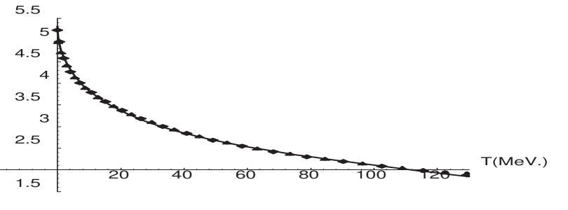
Figure 4: $-\tilde{K}_{0}^{once}(\nu)$ is plotted against $T_{lab}$ in $T_{lab}<125\;MeV.$. The diamonds and triangles are $-\tilde{K}_{0}^{once}(\nu)$ calculated from $X_{0}(\nu)$ of the [sc] and the [fc] fits, whose parameters are listed in Table 1, respectively. The curve is the fit by the spectrum of the long range force in the range $0.6\;MeV.<T_{lab}<125\;MeV.$ .

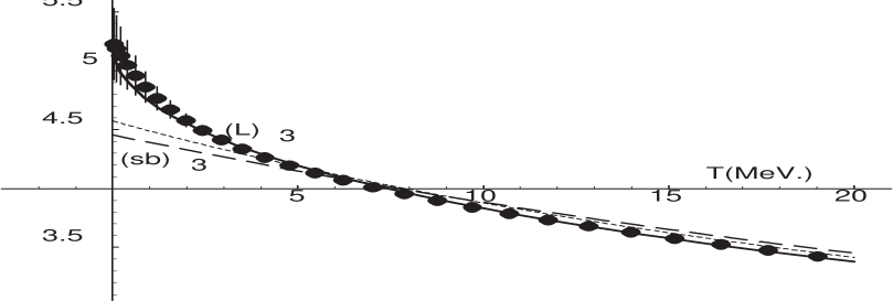
Figure 5: The enlarged graph of $-\tilde{K}_{0}^{once}(\nu)$ of [sc] is plotted in $T_{lab}<20\;MeV.$. The three curves are 3-parameter fits to the data in $0.6\;MeV.<T_{lab}<125\;MeV.$. The curve $(L)_{3}$ is the fit by the spectrum of the long range force, whereas the curves of $(s\;a)_{3}$ (dots) and $(s\;b)_{3}$ (dash) are the fits by the short range potentials.

In the next two sections, $\tilde{K}_{0}^{once}(\nu)$ of Table 3 will be analysed to understand the physical meanings of the cusp at $\nu=0$. In section 4, the cusp will be fitted by the spectrum of the long range force, in which the power $\gamma$ of the threshold behavior of the spectrum will be searched. On the other hand, in section 5 it will be examined whether the short range nuclear potential $V(r)$ can reproduce well the cusp of $\tilde{K}_{0}^{once}(\nu)$.

4 Fits by the Spectrum of the Long Range
Interactions

Figures 4 and 5 indicate that $-\tilde{K}_{0}^{once}(\nu)$ has a cusp pointed upward at $\nu=0$. If there exists the spectrum of the long range force with the attractive sign, appearance of such a cusp in $-\tilde{K}_{0}^{once}(\nu)$ is a natural consequence. In this section, we shall determine the power $\gamma$ and the strength of the threshold behavior of the spectral function at $\nu=0$. More conventional fit will be tried in the next section, in which the possibility to understand the cusp of $-\tilde{K}_{0}^{once}(\nu)$ in terms of the ordinary short range potential of the nuclear force will be considered. The integral representation of the scattering amplitude $\tilde{A}(s,t)$ of the non-OPE part is

$$\tilde{A}(s,t)=\frac{1}{\pi}\int_{t_{0}}^{\infty}dt^{\prime}\frac{\tilde{A}_{t}(s,t^{\prime})}{t^{\prime}-t}\pm\frac{1}{\pi}\int_{u_{0}}^{\infty}du^{\prime}\frac{\tilde{A}_{u}(s,u^{\prime})}{u^{\prime}-u}\quad,$$ (25)

where $t_{0}$ and $u_{0}$ are $4\mu^{2}$ for the short range potential whereas zero for the long range interaction, respectively. The tilde such as $\tilde{A}$ means the function in which the OPE part is already subtracted. Since we are considering the scattering of the identical fermi particles, the signs between the integrations of Eq.(25) are plus for the spin-singlet and minus for the spin-triplet states respectively. Moreover the spectral functions of t and u channels are the same, namely $\tilde{A}_{t}(s,\ast)=\tilde{A}_{u}(s,\ast)$. The partial wave projection of Eq.(25) gives

$$\tilde{h}_{0}(\nu)=\frac{1}{\pi}\int_{0}^{\infty}dt\tilde{A}_{t}(s,t)\frac{1}{2\nu}Q_{0}(1+\frac{t}{2\nu})+(t\rightarrow u)\;.$$ (26)

Therefore the spectral function of the left hand cut of the S-wave amplitude $\tilde{h}_{0}(\nu)$ is

$${\rm Im}\tilde{h}_{0}(\nu)=\frac{1}{4\nu}\{\int_{t_{0}}^{-4\nu}dt\tilde{A}_{t}(s,t)+\int_{u_{0}}^{-4\nu}du\tilde{A}_{u}(s,u)\}\quad for\quad\nu<-t_{0}/4\;.$$ (27)

Let us search the value of the power $\gamma$ of the spectral function of $\tilde{A}_{t}(4m^{2},t)$ at $t=0$ or of ${\rm Im}\tilde{h}_{0}(\nu)$ at $\nu=0$. Because of Eq.(27), the powers $\gamma$’s of these functions are the same. Since $\tilde{A}_{t}(4m^{2},t)$ directly relates to the potential by the Laplace transformation

$$rV(r)=-\frac{1}{\pi m^{2}}\int_{0}^{\infty}dt^{\prime}A_{t}(4m^{2},t^{\prime})e^{-r\sqrt{t^{\prime}}}\quad,$$ (28)

we shall assume the functinal form of $\tilde{A}_{t}(4m^{2},t)$ and search the parameters involved. In the search of the power $\gamma$, three-parameter form of the spectral function will be used, which is

$$\tilde{A}_{t}(4m^{2},t)=\pi C^{\prime}t^{\gamma}\exp[-\beta t]\quad,$$ (29)

where the exponential factor is necessary to make the integration Eq.(26) convergent.

In the search, 68 points of $\tilde{K}_{0}^{once}(\nu)$ in $0.6MeV.<T_{lab}<125MeV.$ are fitted. The fitted points are chosen to be equispacing with respect to $\sqrt{\nu}$, or more precisely $\sqrt{\nu_{n}}=0.025n$ with $5\leq n\leq 72$. The parameters $(\gamma\;,\;\beta\;,\;C^{\prime}\;)$ and $\chi$ of the best fits are

$$\gamma=1.543\;,\quad\beta=0.06264\;,\quad C^{\prime}=0.1762\quad and\quad\chi=0.441 for$$ [sc] (30)

$$\gamma=1.569\;,\quad\beta=0.06544\;,\quad C^{\prime}=0.1734\quad and\quad\chi=0.343 for$$ [ fc ] (31)

respectively. The curves in figures 4 and 5 are the fits of [sc] (full line) and [fc] (dash line) respectively.

In figure 6, $\chi(\gamma)$ is plotted against $\gamma$, in which the full line is [sc] and the dash line is [fc] respectively. $\chi(\gamma)$ is obtained by making the chi-square search for fixed $\gamma$. From the curves, minimum points are determined, which are $\gamma_{min}=1.543\pm 0.055$ and $1.569\pm 0.044$ for [sc] and [fc] respectively. The range of the uncertainty of $\gamma_{min}$ is estimated by the condition that $\chi(\gamma)\leq 1.25\chi_{min}$, in which $\chi_{min}$ is the minimum value of $\chi(\gamma)$. It is remarkable that the value of the power $\gamma$ is close to what is expected in the case of the van der Waals potential of the London type namely to $\gamma=1.50$.

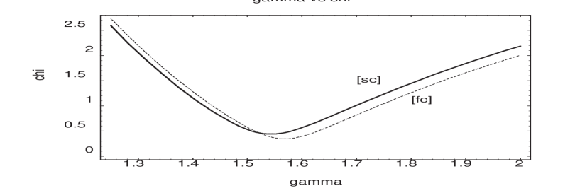
Figure 6: $\chi(\gamma)$ are plotted against $\gamma$. The curves are the fits to the $-\tilde{K}_{0}^{once}(\nu)$ of [sc] (full line) and of [fc] (dash line) respectively. The minimum is close to $\gamma=1.5$ of the Van der Waals force of the London type.

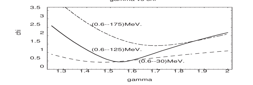
Figure 7: $\chi(\gamma)$ are plotted against $\gamma$ for [sc]. The three curves correspond to the different fitted regions. They are $T_{lab}=$ $(0.6\sim 30)MeV.$ , $(0.6\sim 125)MeV.$ and $(0.6\sim 175)MeV.$ respectively.

However before we discuss about the physical meaning of the value that $\gamma\approx 1.5$, it is necessary to examine the dependency of $\gamma_{min}$ on the fitted range of energy. In figure 7, three curves of $\chi(\gamma)$ with different fitted energy domains are shown. They are $(0.6\sim 30)$ MeV. and $(0.6\sim 175)$ MeV., in addition to the domain $(0.6\sim 125)$ MeV., which was shown in fig.6. The figure indicates that as the energy domain shrinks, $\gamma_{min}$ moves slowly to samaller value. For $0.6MeV.<T_{lab}<30MeV.$ the best fit is that $\gamma_{min}=1.467\pm 0.111$ and $\chi_{min}=0.423$ for [sc]. On the other hand, as the energy region expands, $\gamma_{min}$ increases and moreover the value of $\chi_{min}$ increases rapidly. Therefore the 3-parameter function of Eq.(29) is not suitable for the fit to so many data points. In fact, for the domain $0.6MeV.\leq T_{lab}\leq 175MeV.$, the curve in the figure indicates that $\gamma_{min}=1.695\pm{0.192\atop 0.150}$ and $\chi_{min}=1.410$ for [sc]. Therefore even if we change the energy domain, the power $\gamma$ still remains in the neighborhood of 1.5 .

5 Fits by the Spectral Function of the Short Range Interactions

In the previous section, it was found that the cusp in $\tilde{K}_{0}(\nu)$ obtained in section 3 was reproduced well by the spectral function $\tilde{A}_{t}(4m^{2},t)$ of the long range interaction given in Eqs.(29),(30) and (31). However it is important to ask whether the cusp can be understood also in the framework of the more conventional approach, namely in terms of the spectral function of the short range interaction expected in the meson theory. It is well known that, in the meson theory of the nuclear force, the spectral function of the two-pion exchange is

$$\tilde{A}_{t}(4m^{2},t)=\left\{\begin{array}[]{ll}\qquad 0&{\rm in}\quad t\leq 4\mu^{2}\\ \pi C^{\prime}_{2\pi}(t-4\mu^{2})^{1/2}+\cdots&{\rm in}\quad t>4\mu^{2}\end{array}\right.$$ (32)

, in the neighborhood of the two-pion threshold at $t=4\mu^{2}$. The power 1/2 of Eq.(32) comes from the functional form of the phase volume of the two-particle state exchanged. The coefficient $C^{\prime}_{2\pi}$ can be estimated from the phase shifts of the $\pi$-$N$ and the $\pi$-$\pi$ scatterings by using the generalized unitarity of the dispersion technique[3]. From Eqs.(27) and (32), the spectral function of the left hand cut of $\tilde{h_{0}}(\nu)$, which is the same as that of $\tilde{K_{0}}(\nu)$, becomes

$${\rm Im}\tilde{h}_{0}(\nu^{\prime})=\left\{\begin{array}[]{ll}\qquad 0&{\rm in}\quad\nu^{\prime}>-1\\ \frac{8\pi}{3\nu^{\prime}}C^{\prime}_{2\pi}(-\nu^{\prime}-1)^{3/2}+\cdots&{\rm in}\quad\nu^{\prime}\leq-1\quad.\end{array}\right.$$ (33)

Since the power of the spectral function at the threshold $\nu=-1$ increases to 3/2, the distance of the average location of the spectrum from $\nu=0$ is much larger compared to that of the threshold point. With such a spectral function, it will be not easy to reproduce the cusp of $\tilde{K}_{0}^{once}(\nu)$ observed in $\nu\ll 1$, where in our unit $\nu=1$ corresponds to $T_{lab}=38.83MeV.$ . On the other hand, the updated nuclear potentials are believed to fit well to the precise phase shift data.[13][14][15][16].

In this section, we shall examine the updated nuclear potentials more closely, and in which we shall concentrate on the cusp at $\nu=0$. Among various potentials, we shall choose the regularized Reid potential updated by the Nijmegen group (Reid 93) as an example[15], in which 50 phenomenological parameters are searched to fit to 1787 p-p data and 2514 n-p data in the energy range of $0<T_{lab}<350MeV.$. It is remarkable that by using such potential they achieved excellent fits $\chi^{2}=1.03$ per datum, which is close to the chi-square value $0.99$ of the energy dependent phase shift analysis. In the Reid93, the S-wave potential of the non-OPE part of the p-p scattering involves five parameters:

$$V_{pp}(^{1}S_{0})=A_{2}Y(2)+A_{3}Y(3)+A_{4}Y(4)+A_{5}Y(5)+A_{6}Y(6)\quad,$$ (34)

where the regularized Yukawa functions of the range $1/(p\mu)$ are

$$Y(p)=p\frac{1}{r}[e^{-p\bar{\mu}r}-e^{-\Lambda r}(1+\frac{\Lambda^{2}-p^{2}\bar{\mu}^{2}}{2\Lambda^{2}}\Lambda r)]$$ (35)

and $\bar{\mu}$ is the average masses of the three types of pions and $\Lambda=8\bar{\mu}$. Contrary to the original Reid potential[17], this potential has a characteristic feature that the $Y(2)$ term exists. Such term gives rise to a pole at $t=4\mu^{2}$ in the scattering amplitude $A(s,t)$, whereas in the meson theory $t=4\mu^{2}$ is merely the starting point of the continuous spectrum of the two-pion exchange. Therefore it is not desirable from the point of view of the meson theory to have the $Y(2)$ term in Eq.(34). On the other hand the inclusion of the $Y(2)$ term is necessary, in fitting the very precise low energy data of the p-p scattering, to reduce the the chi-square value. The contradictory situation already indicates the difficulty to reproduce the cusp from the far-away spectral function of the meson theory of the nuclear force.

In figure 5, results of the 3-parameter fits to the data points in $0.6\;MeV.<T_{lab}<125\;MeV.$ are compared. The curve $(L)_{3}$ is the fit by the spectrum of the long range force, while the curves of $(s\;a)_{3}$ and $(s\;b)_{3}$ are the fits by the short range potentials of the Reid types of Eq.(34). The $(s\;a)_{3}$ is the sum of $Y(2)$, $Y(3)$ and $Y(4)$, on the other hand $(s\;b)_{3}$ is the sum of $Y(3)$, $Y(4)$ and $Y(5)$, where $Y(p)$ is the regularized Yukawa potential of range $1/p$ defined in Eq.(35). The $\chi$-values per datum of $(L)_{3}$, $(sa)_{3}$ and $(sb)_{3}$ are 0.441, 1.82 and 3.11 respectively. It is evident that the short range potentials with three parameters cannot reproduce the cusp at $\nu=0$. It is interesting that the inclusion the $Y(2)$ term always reduce the $\chi$-value, this is because the lack of the spectrum of small $t$ is the reason of the deviation from the data points of $\tilde{K}_{0}^{once}(\nu)$.

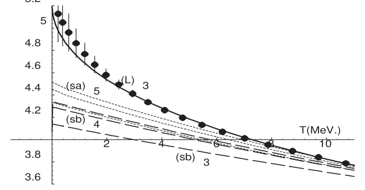
Figure 8: The seven curves are the fits to $\;-\tilde{K}_{0}^{once}(\nu)\;$ of [sc] in the off-cusp region $T_{lab}=$ $(20\sim 125)MeV.$. The fitted curves are then extrapolated to $T_{lab}=0$. The $(L)_{3}$ curve is the 3-parameter fit by the spectrum of the long range force, on the other hand $(s\;a)_{n}$ (dotted curves) and $(s\;b)_{n}$ (dash curves) are the n-paremeter fits by the Reid type potentials. The differences of $(s\;a)_{n}$ and $(s\;b)_{n}$ are that, although $(s\;a)_{n}$ involves $Y(2)$ term, in $(s\;b)_{n}$ the Yukawa term of the longest range is $Y(3)$.

In figure 8, the seven curves are the fits to $\;-\tilde{K}_{0}^{once}(\nu)\;$ of [sc] in the off-cusp region $T_{lab}=$ $(20\sim 125)MeV.$. The fitted curves are then extrapolated to $T_{lab}=0$. The $(L)_{3}$ (full line) curve is the 3-parameter fit by the spectrum of the long range force of Eq.(29) as before, on the other hand $(s\;a)_{n}$ (dotted line) and $(s\;b)_{n}$ (dash line) are the n-paremeter fits by the Reid type potentials. The differences of $(s\;a)_{n}$ and $(s\;b)_{n}$ are that, although $(s\;a)_{n}$ involves $Y(2)$ term, in $(s\;b)_{n}$ the Yukawa term of the longest range is $Y(3)$. In general as the numbers of the parameters $n$ increase, the curves come closer to the data points. However the curves of Fig.8 indicate that the curves of the short range interaction $(s\;b)_{n}$ cannot reproduce the cusp of the data points at $\nu=0$.

In the meson theory, the nearest singularity of $\;-\tilde{K}_{0}^{once}(\nu)\;$ occurs at $\nu=-1$ or in terms of $T_{lab}$ at $-38.83\;MeV.$, which is the threshold of the two-pion exchange spectrum. Since Eq.(33) indicates that the power of of the threshold behavior of the two-pion exchange spectrum at $\nu=-1$ is 3/2, the distance to the average location of the spectrum from the origin is much larger than one. What is important is that the length of our extrapolation ($\sim$ 0.5) is short compared not only to the size of the fitted domain ($\sim 3.0$) but also to the distance to the left hand spectrum ($>1$). Therefore if the analytic structure expected in the meson theory is correct, the extrapolated curve must approximately follow the data points. However figure 8 indicates that this is not the case. On the other hand, the extrapolated curve of the long range force $(L)_{3}$ traces the data point nicely. Therefore we conclude that the analytic structure of the amplitude of the nucleon-nucleon scattering is different from what is expected in the meson theory of the nuclear force, rather the nuclear force involves the large component of the long range force.

6 Strong van der Waals Interaction as a
Candidate of the Nuclear Force

In section 2, we introduced the S-wave Kantor amplitude of the proton-proton scattering $K_{0}(\nu)$, which was free from the singularities of the vacuum polarization and the Coulombic interaction as well as the unitarity cut. By subtracting the one-pion exchange contribution from $K_{0}(\nu)$, the domain of analyticity expands further, and the nearest singularity of the non-OPE Kantor amplitude $\tilde{K}_{0}(\nu)$ occurs at $\nu=-1$, and which is the branch point of the two-pion exchange spectrum. By using the phase shift data of the Nijmegen group[7] [8], the once subtracted non-OPE Kantor amplitude $\tilde{K}_{0}^{once}(\nu)$ defined in Eqs.(6)and (18) was calculated in section 3. The appearance of the cusp at $\nu=0$ is rather surprising, because in the meson theory of the nuclear force, $\tilde{K}_{0}^{once}(\nu)$ is regular at least in $|\nu|<1$.

It turns out that the conventional fits of the spectra of the short range forces cannot reproduce the cusp properly even if the potentials with five parameters given in Eq.(34) are used in the fitting. On the other hand, if we use the spectra of the long range force, three parameters of Eq.(29) are sufficient to reproduce the cusp of $\tilde{K}_{0}^{once}(\nu)$. In summary, the short range condition, that Im$h_{0}(\nu)\equiv 0$ in $\nu>-1$, is too severe to reproduce the cusp in $|\nu|\ll 1$. Therefore it is natural to regard the cusp as an effect of the long range interaction between hadrons. The power $\gamma$ of the threshold behavior was searched in section 4, and it turned out that $\gamma=1.543\pm 0.056$ from the multi-energy data [sc] and $\gamma=1.569\pm 0.046$ determined from the fit [fc], respectively. Since the power $\alpha$ of the asymptotic behavior of the long range potential $V(r)$ is related to the power $\gamma$ by $\alpha=2\gamma+3$, the values of $\gamma$ imply $\alpha=6.09\pm 0.11$ and $\alpha=6.17\pm 0.09$ for [sc] and [fc] respectively.

It is remarkable that the values of $\alpha$ are close to that of the van der Waals potential of the London type ( $\alpha=6$ ). Although $\alpha$ can assume any value from $-1$ (Coulomb) to infinity (Yukawa), Nature chooses a special value in the neighborhood of $\alpha=6$. Therefore it is difficult to believe the occurrence of the value $\alpha=5.98\sim 6.26$ is merely accidental, rather the ordinary mechanism to produce the van der Waals interaction must be working. It is well-known in the atomic and molecular physics that, when the underlying Coulombic force exists, the dipole-dipole interaction occurs between the neutral composite particles, and the two-step process of such interactions causes the attractive potential[18]. The form of the potential between particle 1 and particle 2 is

$$V(R)=-\mathop{{\sum}^{\prime}}_{n}\frac{(H^{\prime})_{0n}(H^{\prime})_{n0}}{E_{n}-E_{0}}\quad,$$ (36)

where $H^{\prime}$ is the hamiltonian of the dipole-dipole interaction

$$H^{\prime}=\frac{{}^{\ast}e^{2}}{R^{3}}(x_{1}x_{2}+y_{1}y_{2}-2z_{1}z_{2})\quad,$$ (37)

in which ${}^{\ast}e^{2}$ is the strength of the underlying Coulombic interaction.

It is important to notice that each term in the summation of Eq.(36) is positive definite. Therefore if we replace all the denominators $(E_{n}-E_{0})$ in Eq.(36) by the first excitation energy $(\Delta E_{1})$, then by using the closure property the upper bound of the strength $C_{6}$ of the van der Waals potential, which is introduced by $V(R)=-C_{6}/R^{6}+\cdots$, is obtained. It is[18]

$$C_{6}<\frac{R^{6}({H^{\prime}}^{2})_{00}}{(\Delta E_{1})}=\frac{2}{3}\frac{{}^{\ast}e^{4}}{(\Delta E_{1})}\;\overline{r_{1}^{2}}\;\;\overline{r_{2}^{2}}\;\;.$$ (38)

On the other hand, if we retain only the terms of the first excited states in the summation, Eq.(36) gives the lower bound of $C_{6}$, namely

$$C_{6}>\frac{2}{3}\frac{{}^{\ast}e^{4}}{(\Delta E_{1})}\tilde{R_{1}}^{2}\;\tilde{R_{2}}^{2}\quad,$$ (39)

where $\tilde{R_{i}}^{2}$ relates to the dipole transition amplitude $\tilde{z}$ by

$$\tilde{R}^{2}=3|\tilde{z}|^{2}\qquad{\rm with}\quad\tilde{z}=\int d^{3}r\psi^{\ast}_{1,1,0}\;(r\cos\theta)\;\psi_{0,0,0}\;.$$ (40)

Since we know the value of $C_{6}$, Eqs.(38) and (39) will be used in turn to give the lower and the upper bounds of the strength of the underlying Coulombic force ${}^{\ast}e^{2}$ respectively, and which are

$$\sqrt{\frac{3}{2}C_{6}(\Delta E_{1})}\quad\frac{1}{\overline{r^{2}}}<\;^{\ast}\!e^{2}<\sqrt{\frac{3}{2}C_{6}(\Delta E_{1})}\quad\frac{1}{\tilde{R}^{2}}\;$$ (41)

The numerical values of $C^{\prime}$ and $\beta$ of Eq.(29) for $\gamma=1.5$ are obtained by shrinking the energy range to be fitted. The results are

$$\gamma =1.5 \;,\quad\beta=0.0547\quad and\quad C^{\prime}=0.174\qquad for\quad[sc]$$ (42)

$$\gamma =1.5 \;,\quad\beta=0.0541\quad and\quad C^{\prime}=0.172\qquad for\quad[\;fc\;]$$ (43)

in the unit of the neutral pion mass, and the energy range of the fits are $(0.6\sim 34)$ MeV. and $(0.6\sim 39)$ MeV. for [sc] and [ fc ] respectively. Since the coefficient $C_{\alpha}$ of the asymptotic potential is

$$C_{\alpha}=C^{\prime}\frac{2\Gamma(\alpha-1)}{m^{2}}\qquad{\rm with}\quad\alpha=2\gamma+3\quad,$$ (44)

$C_{6}=0.9933C^{\prime}$ in our unit. If we use the mass difference of $\Delta(1232)$ and $N$ as the first excitation energy, namely $\Delta E=2.18$, then the lower bound of ${}^{\ast}e^{2}$ becomes

$${}^{\ast}e^{2}>\frac{\sqrt{3.27C^{\prime}}}{\overline{r_{1}^{2}}}.$$ (45)

To go further we need the size of the composite particle, the radius of proton in particular. Although we do not have much information on the radius, we shall consider two cases. In the first case, $\overline{r_{1}^{2}}$ is $(0.7{\rm fm.})^{2}$, which comes from the nucleon form factor. In another case $\overline{r_{1}^{2}}$ is set equal to $\beta$ of Eqs.(42) and (43), because at the range $r=\sqrt{\beta}$ the potential starts to deviate appreciablly from the asymptotic form of the van der Waals potential of $V(R)\sim-C_{6}/R^{6}$ and therefore $\sqrt{\beta}$ may be regarded as the size of the composite particle. The results are :

$${}^{\ast}e^{2}>3.27\qquad ( {\rm from\;the\;form\;factor}\;)$$

$${}^{\ast}e^{2}>13.8\qquad ( {\rm from}\quad\overline{r_{1}^{2}}=\beta\;)\;.$$

As it is expected, the underlying Coulombic force is super-strong, because the induced van der Waals force has already the order of magnitude of the strong interaction.

The coupling constants ${}^{\ast}e^{2}$ of the QED and the QCD are too small, they are $(137.036)^{-1}$ and 0.32 respectively. On the other hand, the Coulombic force of the magnetic monopoles is an imortant candidate of the underlying Coulombic interaction. It is well-known from the charge quantization condition of Dirac that[19]

$${}^{\ast}e^{2}=\frac{137.036}{4}.$$ (46)

Therefore ${}^{\ast}e^{2}$ of the magnetic charge is large enough to satisfies the condition of the lower bound, moreover it is not very large compared to the value of the lower bound. This situation is satisfactory, because the upper bound of Eq.(41) must have the value of the same order of magnitude as the lower bound.

Since the Coulombic interaction between the magnetic monopoles is a suitable candedite of the underlying dynamics of the nuclear force, it is worthwhile to repeat briefly the magnetic monopole model of hadron[2]. Although it is overshadowed by the QCD, it still has virtue to be considered. The monopole model of hadron is essentially the quark model, in which the quarks bear the magnetic charges. Such a fundamental particle is often called dyon, since it is doublly charged, namely electrically and magnetically charged. Because of the superstrong Coulombic force between magnetic charges, the dyons form the bound states of magnetic charge zero, and such composite particles are identified with the hadrons. In a sense, hadrons are regarded as “ magnetic atoms ” in this model[3]. Therefore it is not surprising to observe the strong van der Waals forces between hadrons. In this article we actually observed the strong van der Waals interaction in the proton-proton scattering. Since the van der Waals interaction is universal[20], we may expect to observe such a force also in other scattering processes. However because of the lower precision of the data, the elimination of the two-pion exchange cut is necessary at least in the threshold region of the spectrum. After carrying out such eliminations, we can actually observe the long range force in the P-wave amplitudes of the $\pi$-$N$ and the $\pi$-$\pi$ scatterings[21][22].

7 Remarks and Comments

In this paper we searched for the long range force in the S-wave amplitude of the proton-proton scattering. In order to see the extra singularity of the long range force in $h_{0}(\nu)$ at $\nu=0$ as clearly as possible, we constructed a regular function $K_{0}(\nu)$ from the modified effective range function $X_{0}(\nu)$ of the proton-proton scattering, where the function $K_{0}(\nu)$ does not have the normal singularities in the neighborhood of $\nu=0$. By separating the OPE part and then making the once subtracted function $\tilde{K}_{0}^{once}(\nu)$, it becomes much easier for us to observe the extra singularity at $\nu=0$ when it exists. It is impressive to observe that $\tilde{K}_{0}^{once}(\nu)$ has a sharp cusp at $\nu=0$, and the form of which is close to the square root type, namely to $\tilde{K}_{0}^{once}(\nu)=(C^{\prime\prime}_{0}+C^{\prime\prime}\sqrt{\nu})$ with positive $C^{\prime\prime}$. The $\sqrt{\nu}$ singularity is exactly what is expected in the van der Waals interaction of the London type. Moreover the observed sign of $C^{\prime\prime}$ indicates that the long range force is attractive.

If we state it more precisely, when the spectral function has the form of $A_{t}(4m^{2},t)=\pi C^{\prime}t^{\gamma}\exp(-\beta t)$, the chi-square fit to the multi-energy phase shift data[7] [8] determines the three parameters involved. They are $\gamma=1.54$, $\beta=0.063$ and $C^{\prime}=0.175$ in the unit of the neutral pion mass. It is interesting to see that the spectral function $A_{t}(4m^{2},t)$ has a peak at $\sqrt{t}=4.9$ namely at 660MeV.. On the other hand, the location of the peak of the spectrum $A_{t}(4m^{2},t)/t$ of the once subtracted amplitude is $\sqrt{t}=2.93$ or 395MeV.. When we do not need the very precise description of the low energy phase shifts, the spectral function can be replaced by a $\delta$-function located somewhere between 400 and 650MeV.. Such a $\delta$-function may correspond to the fictitious $\sigma$-meson of the one-boson exchange model of the nuclear potential[23][24] [25].

Since the power $\gamma$ of the threshold behavior of the spectral function $A_{t}(4m^{2},t)$ is close to that of the van der Waals force of the London type, we may assume that the ordinary mechanism, which produce the van der Waals force, is working. Then the strength ${}^{\ast}e^{2}$ of the underlying Coulombic force can be estimated. This is possible because there are the well-known inequalities on the coefficient $C_{6}$ of the van der Waals potential[18], in particular the upper bound of which is obtained by using the strength ${}^{\ast}e^{2}$ and the radius $(\;\overline{r^{2}}\;)^{1/2}$ of the composite particle. Since we know the strength $C_{6}$ of the van der Waals potential from the fitting, the inequality gives instead the lower bound of ${}^{\ast}e^{2}$, which depends on size of the composite state. For $(\;\overline{r^{2}}\;)^{1/2}=0.5$, which is obtained by the measurement of the nucleon form factor, we obtain ${}^{\ast}e^{2}>3.3$, whereas for $(\;\overline{r^{2}}\;)^{1/2}=\sqrt{\beta}=0.25$, we obtain ${}^{\ast}e^{2}>14$. In any case, the underlying Coulombic force is super-strong. Among the interactions of the Coulombic form, the force between the magnetic monopoles satisfies this inequalty, because ${}^{\ast}e^{2}=137.036/4\;$ due to the charge quantization condition of Dirac[19]. Therefore the dyon model of hadron, in which the constituent particle dyon bears the magnetic charge as well as the electric charge, must be an important candidate of the model of hadron[2].

Finally, in order to confirm the long range force in the proton-proton scattering, it is desirable to observe directly the difference of the interference patterns by measuring precisely the angular distributions of the cross section in the low energy experiments. Our proposal is to observe the interference between the repulsive Coulomb force and the attractive long range interaction obtained in the present article. Since the interference pattern of the conventional short range foece and the Coulomb force is known, the difference can be predicted by using the values of parameters $\gamma$, $\beta$ and $C$. It turns out that the most favorable energy is in $T_{lab}=25MeV.\sim 40MeV.$. Since the relative deviation, namely $\Delta(d\sigma/d\Omega)\cdot(d\sigma/d\Omega)^{-1}$, has a dip around $\theta_{c.m.}=10^{\circ}$ with the depth $\sim 0.3\%$, there exist two challenging requirements in the measurements. They are the accuracy and the domain of $\theta_{c.m.}$. However since the shape of the interference pattern is important, there is no severe conditions on the normalization of the cross section. Details will be published in a separate paper.

References

- [1] H. Yukawa , Proc. Phys. Math. Soc. Japan 17 , 98 , (1935)
-
[2]
J. Schwinger , Science 165 ,757 , (1969)
A. O. Barut , Phys. Rev. D3 , 1747 , (1971)
T. Sawada , Phys. Lett. B43 , 517 , (1973) -
[3]
T. Sawada , Phys. Lett. 43B , 517 , (1973)
T. Sawada , Nucl. Phys. B71 , 82 , (1974)
T. Sawada , Prog. Theor. Phys. 59 , 149 , (1978) - [4] Ch. Thomann, J. E. Benn and S. Münch Nucl. Phys. A303 , 457 , (1978)
- [5] P. B. Kantor , Phys. Rev. Lett. 12 , 52 , (1964)
- [6] L. Heller , Phys. Rev. 120 , 627 , (1960)
- [7] J.R. Bergervoet, P.C. van Campen, W.A. van der Sanden and J.J. de Swart , Phys. Rev. C38 , 15 , (1988)
- [8] J.R. Bergervoet, P.C. van Campen, R.A.M. Klomp, J.L. de Kok, T.A. Rijken, V.G.J. Stoks and J.J. de Swart , Phys. Rev. C41 , 1435 , (1990)
- [9] V.G.J. Stoks , R.A.M. Klomp , M.C.M. Rentmeester and J.J. de Swart , Phys. Rev. C48 , 792 , (1993)
-
[10]
R. A. Arndt, L. D. Roper, R. A. Bryan, R. B. Clark,
B. J. DerWest and P. Signell , Phys. Rev. D28 , 97 , (1983)
R. A. Arndt, J. S. Hyslop III and L. D. Roper, Phys. Rev. D35 , 128 , (1987)
R. A. Arndt, L. D. Roper, R. L. Workman and M. W. McNaughton , Phys. Rev. D45 , 3995 , (1992) - [11] O. Dumbrajs, R. Koch, H. Pilkuhn, G. C. Oades, H. Behrens, J. J. DeSwart and P. Kroll , Nucl. Phys. B216 , 277 , (1983)
- [12] D.V.Bugg and R.Machleidt , Phys. Rev. C52 , 1203 , (1995)
- [13] M.Lacombe , B.Loiseau , J.M.Richard , R.Vinh Mau , J.Côté , P.Pirès and R.de Tourreil , Phys. Rev. C21 , 861 , (1980)
-
[14]
R.Machleidt , K. Holinde and Ch. Elster ,
Phys. Rep. 149 , 1 , (1987)
R.Machleidt , Adv.Nucl.Phys. 19 , 189 , (1989)
J.Heidenbauer and K.Holinde , Phys.Rev. C40 , 2465 , (1989) -
[15]
V.G.J. Stoks , R.A.M. Klomp , C.P.F.Terheggen
and J.J. de Swart , Phys. Rev. C49 , 2950 , (1994)
M.M.Nagels, T.A. Rijken and J.J. de Swart , Phys. Rev. D17 , 768 , (1978) - [16] R.B.Wiringa, V.G.J. Stoks , R.Schiavilla , Phys. Rev. C51 , 38 , (1995)
- [17] R.V.Reid Jr. , Ann Phys.(N.Y.) 50 , 411 , (1968)
- [18] L.Pauling and E.B.Wilson Jr. , “ Introduction to Quantum Mechanics ” , McGraw-Hill Book Company Inc. , (1935)
- [19] P. A. M. Dirac , Proc. R. Soc. London A133 , 60 , (1931)
- [20] T. Sawada , Phys. Lett. B100 , 50 , (1981)
- [21] T. Sawada , Nuovo Cimento 62A , 207 , (1981)
-
[22]
T. Sawada , Prog. Theor. Phys. 63
, 2016 , (1980)
T. Sawada , Phys. Lett. B225 , 291 , (1989) - [23] M.G.Fuda and Y.Zhang , Phys. Rev. C51 , 23 , (1995)
-
[24]
P.Estabrooks and A.D.Martin , Nucl.Phys. B79
, 301 , (1974)
C.D.Froggatt and J.L.Petersen , Nucl.Phys. B129 , 89 , (1977)
O.O.Patarakin , V.N.Tikhonov and K.N.Mukhin , Nucl.Phys. A598 , 335 , (1996) - [25] T.Sawada, Frascati Physics Series XV, 223, (1999)