Do Neutrinos Decay?

Abstract

If neutrinos have masses and mixings, in general some will decay. In models with new particles and new couplings, some decay modes can be fast enough to be of phenomenological interest.

I Introduction

It is generally agreed that most probably neutrinos have non-zero masses and non-trivial mixings. This belief is based primarily on the evidence for neutrino mixings and oscillations from the data on atmospheric neutrinos and on solar neutrinosbarger .

If this is true, then in general the heavier neutrinos are expected to decay into the lighter ones via flavor changing processes. The only questions are (a) whether the lifetimes are short enough to be phenomenologically interesting (or are they too long?) and (b) what are the dominant decay modes.

Throughout the following discussion, to be specific, I will assume that the neutrino masses are at most of order of a few eV. There are interesting things to be done with heavier decaying neutrinos which we will not discuss here todaykawasaki .

II Radiative Decays

For eV neutrinos, the only radiative decay modes possible are $\nu_{i}\rightarrow\nu_{j}+\gamma$. They can occur at one loop level in SM (Standard Model). The decay rate is given bypetcov :

$$\Gamma=\frac{9}{16}\ \frac{\alpha}{\pi}\ \frac{G^{2}_{F}}{128\pi^{3}}\ \frac{\left(\delta m_{ij}^{2}\right)^{3}}{m_{i}}\left|\sum_{\alpha}\ U_{i\alpha}^{*}\ U_{\alpha j}\ \left(\frac{m_{\alpha}^{2}}{m^{2}_{W}}\right)\right|^{2}$$ (1)

where $\delta m^{2}_{ij}=m^{2}_{i}-m^{2}_{j}$ and $\alpha$ runs over $e,\mu$ and $\tau$. When $m_{i}\gg m_{j},m_{i}\sim O(eV)$ and for maximal mixing $(4U^{*2}_{i\alpha}U^{2}_{\alpha j})\sim O(1)$ and $(\alpha\cong\tau)$ one obtains for $\Gamma$

$$\Gamma_{SM}\sim 10^{-45}\ sec^{-1}$$ (2)

which is far too small to be interesting. If the dominant contribution is from electron (rather than $\tau$) then there is enhancement in matter (due to the electrons present) by a factornieves

$$10^{24}\left(\frac{\rho_{e}}{10^{24}(cc)^{-1}}\right)\left(\frac{1eV}{m_{i}}\right)^{4}\ F$$ (3)

where the function $F$ tends to $4m_{i}/E_{i}$ for relativistic $\nu^{\prime}_{i}s_{i}$ and this enhancement can be as large as $10^{16}$.

The decay mode $\nu_{i}\rightarrow\nu_{j}+\gamma$ comes from an effective coupling which can be written as:

$$\left(\frac{e}{m_{i}+m_{j}}\right)\bar{\psi}_{j}\sigma_{\mu\nu}(C+D\gamma_{5})\psi_{i}\ F{{}_{\mu}\nu}$$ (4)

Let us define $k_{ij}$ as

$$k_{ij} = \left(\frac{e}{m_{i}+m_{j}}\right)\sqrt{\mid C\mid^{2}+\mid D\mid^{2}}$$

$$\equiv k_{0}\mu_{B}$$

where $\mu_{B}=e/2m_{e}$. Since the experimental bounds on $\mu_{\nu i}$, the magnetic moments of neutrinos, come from reactions such as $\nu_{e}e\rightarrow e``\nu^{\prime\prime}$ which are not sensitive to the final state neutrinos; the bounds apply to both diagonal as well as transition magnetic moments and so can be used to limit $k^{i}_{0}$ and the corresponding lifetimes. The current bounds areparticle :

$$k^{e}_{0}\ <\ 10^{-10}$$ (6)

$$k^{\mu}_{0}\ <\ 7.4.10^{-10}$$

$$k^{\tau}_{0}\ <\ 5.4.10^{-7}$$

For $m_{i}\gg m_{j}$, the decay rate for $\nu_{i}\rightarrow\nu_{j}+\gamma$ is given by

$$\Gamma=\frac{\alpha}{2m_{e}^{2}}\ m_{i}^{3}\ k_{0}^{2}$$ (7)

This, in turn, gives indirect bounds on radiative decay lifetimes for $O(eV)$ neutrinos of:

$$\tau_{\nu_{e}}\ >\ 5.10^{18}\ \mbox{sec}$$ (8)

$$\tau_{\nu_{\mu}}\ >\ 5.10^{16}\ \mbox{sec}$$

$$\tau_{\nu_{\tau}}\ >\ 2.10^{11}\ \mbox{sec}$$

There is one caveat in deducing these bounds. Namely, the form factors C and D are evaluated at $q^{2}\sim O(eV^{2})$ in the decay matrix elements whereas in the scattering from which the bounds are derived, they are evaluated at $q^{2}\sim O(MeV^{2})$. Thus, some extrapolation is necessary. It can be argued that, barring some bizarre behaviour, this is justifiedfrere .

There are other bounds on radiative lifetimes of neutrinos which are all based on non-observation of the final state $\gamma$-ray. The most direct observational bounds from reactor and accelerators areparticle :

$$\tau(\nu_{e})\ >300\ s$$ (9)

$$\tau(\nu_{\mu})\ >15.4\ s$$

There are other more indirect boundsparticle . From cosmology:

$$\tau>2.10^{21}\ s.$$ (10)

From x-ray and $\gamma$-ray fluxes:

$$\tau>7.10^{9}\ s.$$ (11)

Here we have set $m_{i}\sim O(eV)$. All these bounds depend on assuming that $m_{i}\gg m_{j}$ in the mode $\nu_{i}\rightarrow\nu_{j}+\gamma$. The bounds are not valid if there is near degeneracy; since in this case the $\gamma$-ray can be soft.

III The Sciama Model

Dennis Sciama proposed an intriguing and imaginative scenario for radiative decay of a neutrino about 10 years agosciama . It went thru several metamorphoses; starting out as a decay mode $\nu_{\tau}\rightarrow\nu_{\mu}+\gamma$ and ending up most recently as $\nu_{st}\rightarrow\nu^{\prime}_{st}+\gamma$mohapatra .

The proposal was this: (a) suppose the decay $\nu_{\alpha}\rightarrow\nu_{\beta}+\gamma$ takes place, (b) the mass of $\nu_{\alpha}(m_{\nu\alpha})$ is $\sim 27.4$ eV, and $m_{\nu_{\alpha}}\gg m_{\nu_{\beta}},$ (c) thus $E_{\gamma}\approx\ 13.7$ eV for a slow moving $\nu_{\alpha}$; (d) the lifetime by this mode for $\nu_{\alpha}$ is about $2.10^{23}$ sec. These properties are consistent with all the bounds. The purpose was to account for the anomalous amount of ionised $H$ in interstellar space. The energy of the decay photon is just right to ionise hyrogen; and the lifetime is chosen so as to provide the required amount of ionization.

After a lengthy innings (of 10 years), it appears that the Sciama model is finally ruled out. The most recent evidence against it is the non-observation of the line at 911 Å(corresponding to 13.7 eV) with the predicted intensitybowyer .

IV Invisible Decays

A decay mode with essentially invisible final states which does not involve any new particles is the three body neutrino decay mode. The decay is $\nu_{i}\rightarrow\nu_{j}\nu_{j}\bar{\nu}_{j}$. This decay, like the radiative mode, can occur at one loop level in SM. With a mass pattern $m_{i}\gg m_{j}$ the decay rate can be written as

$$\Gamma=\frac{\epsilon^{2}\ G^{2}_{F}\ m_{j}^{5}}{192\pi^{3}}$$ (12)

In the SM at one loop level, with the internal $\tau$ dominating, the value of $\epsilon^{2}$ is given bylee

$$\epsilon_{SM}^{2}=\frac{3}{16}\left(\frac{\alpha}{\pi}\right)^{2}\left(\frac{m_{\tau}}{m_{W}}\right)^{4}\left\{\ell n\left(\frac{m_{\tau}^{2}}{m_{w}^{2}}\right)\right\}^{2}\left(U_{\tau j}\ U^{*}_{\tau i}\right)^{2}$$ (13)

With maximal mixing $\epsilon^{2}_{SM}\approx 3.10^{-12}$. Even if $\epsilon$ were as large as 1 with new physics contributions; it only gives a value for $\Gamma$ of $5.10^{-35}\ sec^{-1}$. Hence, this decay mode will not yield decay rates large enough to be of interest. It is worth noting that the current experimental bound on $\epsilon$ is quite poor: $\epsilon<O(100)$bilenky .

V $\nu_{\alpha_{L}}\rightarrow\nu_{\beta_{L}}+\chi$

If the only new particle introduced is an I=0, L=0, J=0, massless particle such as a Goldstone boson (familon), then a new decay mode is possible:

$$\nu_{\alpha_{L}}\rightarrow\nu_{\beta_{L}}+\chi$$ (14)

which arises from a coupling of the form

$$g_{p}\bar{\psi}_{\beta_{L}}\gamma_{\mu}\psi_{\alpha_{L}}\partial_{\mu}\chi$$ (15)

with a decay rate

$$\Gamma=\frac{g^{2}_{p}m^{3}_{\alpha}}{16\pi}$$ (16)

$SU(2)_{L}$ symmetry predicts a similar coupling for the charged leptons with decay mode $\ell_{\alpha}\rightarrow\ell_{\beta}+\chi$. Thus the $\nu_{\alpha}$ lifetime is related to the B.R. $(\ell_{\alpha}\rightarrow\ell_{\beta}+\chi)$ by

$$\tau_{\nu_{\alpha}}=\frac{\tau_{\ell\alpha}}{B.R.(\ell_{\alpha}\rightarrow\ell_{\beta}+\chi)}\left(\frac{m_{\nu_{\alpha}}}{m_{\ell_{\alpha}}}\right)^{-3}$$ (17)

The current bounds on $\mu$ and $\tau$ branching ratios areparticle ; jodidio

$$B.R.(\mu\rightarrow e\chi)\ <2.10^{-6}$$ (18)

$$B.R.(\tau\rightarrow\mu\chi)\ <7.10^{-6}$$

and lead to

$$\tau_{\nu_{\mu}}>10^{24}\ s$$ (19)

$$\tau_{\nu_{\tau}}>10^{20}\ s.$$

Coupling to a scalar field with $I=1/2$, $L=0$ would have the same constraint as above; and in addition would require fine tuning to avoid mixing with the SM Higgs.

VI Fast Invisible Decays

The only possibility for fast invisible decays of neutrinos seems to lie with Majoron models. There are two classes of models; the I=1 Gelmini-Roncadelligelmini majoron and the I=0 Chikasige-Mohapatra-Pecceichikasige majoron. In general, one can choose the majoron to be a mixture of the two; furthermore the coupling can be to flavor as well as sterile neutrinos. The effective interaction is of the form:

$$g_{\alpha}\bar{\nu}_{\beta}^{c}\nu_{\alpha}\ J$$ (20)

giving rise to decay:

$$\nu_{\alpha}\rightarrow\bar{\nu}_{\beta}\ +J$$ (21)

where $J$ is a massless $J=0\ L=2$ particle; $\nu_{\alpha}$ and $\nu_{\beta}$ are mass eigenstates which may be mixtures of flavor and sterile neutrinos. Models of this kind which can give rise to fast neutrino decays and satisfy the bounds below have been discussed by Valle, Joshipura and othersvalle . These models are unconstrained by $\mu$ and $\tau$ decays which do not arise due to the $\Delta L=2$ nature of the coupling. The I=I coupling is constrained by the bound on the invisible $Z$ widthkawasaki ; and requires that the Majoron be a mixture of I=1 and I=0. The couplings of $\nu_{\mu}$ and $\nu_{e}\ (g_{\mu}$ and $g_{e})$ are constrained by the limits on multi-body $\pi,k$ decays ${\pi\rightarrow\mu\nu\nu\nu}$ and $K\rightarrow\mu\nu\nu\nu$ and on $\mu-e$ university violation in $\pi$ and K decaysbarger1 .

Granting that models with fast, invisible decays of neutrinos can be constructed, can such decay modes be responsible for any observed neutrino anomaly?

We assume a component of $\nu_{\alpha},$ i.e., $\nu_{2}$, to be the only unstable state, with a rest-frame lifetime $\tau_{0}$, and we assume two flavor mixing, for simplicity:

$$\nu_{\alpha}=cos\theta\nu_{2}\ +sin\theta\nu_{1}$$ (22)

with $m_{2}>m_{1}$. From Eq. (2) with an unstable $\nu_{2}$, the $\nu_{\alpha}$ survival probability is

$$P_{\alpha\alpha} = sin^{4}\theta\ +cos^{4}\theta{\rm exp}(-\alpha L/E)$$

$$+ 2sin^{2}\theta cos^{2}\theta{\rm exp}(-\alpha L/2E)cos(\delta m^{2}L/2E),$$

where $\delta m^{2}=m^{2}_{2}-m_{1}^{2}$ and $\alpha=m_{2}/\tau_{0}$. Since we are attempting to explain neutrino data without oscillations there are two appropriate limits of interest. One is when the $\delta m^{2}$ is so large that the cosine term averages to 0. Then the survival probability becomes

$$P_{\mu\mu}=sin^{4}\theta\ +cos^{4}\theta{\rm exp}(-\alpha L/E)$$ (24)

Let this be called decay scenario A. The other possibility is when $\delta m^{2}$ is so small that the cosine term is 1, leading to a survival probability of

$$P_{\mu\mu}=(sin^{2}\theta+cos^{2}\theta{\rm exp}(-\alpha L/2E))^{2}$$ (25)

corresponding to decay scenario B. Decay models for both kinds of scenarios can be constructed; although they require fine tuning and are not particularly elegant.

The possibility of solar neutrinos decaying to explain the discrepancy is a very old suggestionpakvasa . The most recent analysis of the current solar neutrino data finds that no good fit can be found: $U_{ei}\approx 0.6$ and $\tau_{\nu}$ (E=10 MeV) $\sim 6$ to 27 sec. come closestacker . The fits become acceptable only if the suppression of the solar neutrinos is energy independent as proposed by several authorsharrison (which is possible if the Homestake data are excluded from the fit). The above conclusions are valid for both the decay scenarios A as well as B.

For atmospheric neutrinos, assuming neutrino decay scenario A, it was found that it is possible to choose $\theta$ and $\alpha$ to provide a good fit to the Super-Kamiokande L/E distributions of $\nu_{\mu}$ events and $\nu_{\mu}/\nu_{e}$ event ratiobarger2 . The best-fit values of the two parameters are $cos^{2}\theta\sim 0.87$ and $\alpha\sim 1GeV/D_{E},$ where $D_{E}=12800$ km is the diameter of the Earth. This best-fit $\alpha$ value corresponds to a rest-frame $\nu_{2}$ lifetime of

$$\tau_{0}=m_{2}/\alpha\sim\frac{m_{2}}{(1eV)}\times 10^{-10}s.$$ (26)

However, it was then shown that the fit to the higher energy events in Super-K (especially the upcoming muons) is quite poorlipari . The reason that the inclusion of high energy upcoming muon events makes the fits poorer is very simple. In the decay A scenario, due to time dilation, the decay is suppressed at high energy and there is hardly any depletion of $\nu_{\mu}^{\prime}s$, contrary to observation.

Turning to decay scenario B, consider the following possibilitybarger3 . The three states $\nu_{\mu},\nu_{\tau},\nu_{s}$ (where $\nu_{s}$ is a sterile neutrino) are related to the mass eigenstates $\nu_{2}\nu_{3}\nu_{4}$ by the approximate mixing matrix.

$$\left(\begin{array}[]{c}\nu_{\mu}\\ \nu_{\tau}\\ \nu_{s}\end{array}\right)=\left(\begin{array}[]{ccc}\cos\theta&\sin\theta&0\\ -\sin\theta&\cos\theta&0\\ 0&0&1\end{array}\right)\left(\begin{array}[]{c}\nu_{2}\\ \nu_{3}\\ \nu_{4}\end{array}\right)$$ (27)

and the decay is $\nu_{2}\to\bar{\nu}_{4}+J$. The electron neutrino, which we identify with $\nu_{1}$, cannot mix very much with the other three because of the more stringent bounds on its couplingsbarger1 , and thus our preferred solution for solar neutrinos would be small angle matter oscillations.

In this case the $\delta m_{23}^{2}$ in Eq. (23) is not related to the $\delta m_{24}^{2}$ in the decay, and can be very small, say $<10^{-4}\rm\,eV^{2}$ (to ensure that oscillations play no role in the atmospheric neutrinos). Then the oscillating term is 1 and $P(\nu_{\mu}\to\nu_{\mu})$ is given by Eq. (25).

In order to compare the predictions of this model with the standard $\nu_{\mu}\leftrightarrow\nu_{\tau}$ oscillation model, we have calculated with Monte Carlo methods the event rates for contained, semi-contained and upward-going (passing and stopping) muons in the Super-K detector, in the absence of ‘new physics’, and modifying the muon neutrino flux according to the decay or oscillation probabilities discussed above. We have then compared our predictions with the SuperK data fukuda , calculating a $\chi^{2}$ to quantify the agreement (or disagreement) between data and calculations. In performing our fit (see Ref. barger3 for details) we do not take into account any systematic uncertainty, but we allow the absolute flux normalization to vary as a free parameter $\beta$.

The decay model of Equation (24) above gives a very good fit with a minimum $\chi^{2}=33.7$ (32 d.o.f.) for the choice of parameters

$$\tau_{\nu}/m_{\nu}=63\rm~{}km/GeV,\ \cos^{2}\theta=0.30$$ (28)

and normalization $\beta=1.17$.

In Fig. 1 we compare the best fits of the two models considered (oscillations and decay) with the SuperK data. In the figure we show (as data points with statistical error bars) the ratios between the SuperK data and the Monte Carlo predictions calculated in the absence of oscillations or other form of ‘new physics’ beyond the standard model. In the six panels we show separately the data on $e$-like and $\mu$-like events in the sub-GeV and multi-GeV samples, and on stopping and passing upward-going muon events. The solid (dashed) histograms correspond to the best fits for the decay model ($\nu_{\mu}\leftrightarrow\nu_{\tau}$ oscillations). One can see that the best fits of the two models are of comparable quality. The reason for the similarity of the results obtained in the two models can be understood by looking at Fig. 2, where we show the survival probability $P(\nu_{\mu}\to\nu_{\mu})$ of muon neutrinos as a function of $L/E_{\nu}$ for the two models using the best fit parameters. In the case of the neutrino decay model (thick curve) the probability $P(\nu_{\mu}\to\nu_{\mu})$ monotonically decreases from unity to an asymptotic value $\sin^{4}\theta\simeq 0.49$. In the case of oscillations the probability has a sinusoidal behaviour in $L/E_{\nu}$. The two functional forms seem very different; however, taking into account the resolution in $L/E_{\nu}$, the two forms are hardly distinguishable. In fact, in the large $L/E_{\nu}$ region, the oscillations are averaged out and the survival probability there can be well approximated with 0.5 (for maximal mixing). In the region of small $L/E_{\nu}$ both probabilities approach unity. In the region $L/E_{\nu}$ around 400 km/GeV, where the probability for the neutrino oscillation model has the first minimum, the two curves are most easily distinguishable, at least in principle.

Decay Model

There are two decay possibilities that can be considered: (a) $\nu_{2}$ decays to $\bar{\nu}_{4}$ which is dominantly $\nu_{s}$ with $\nu_{2}$ and $\nu_{3}$ mixtures of $\nu_{\mu}$ and $\nu_{\tau}$, as in Eq. (27), and (b) $\nu_{2}$ decays into $\bar{\nu}_{4}$ which is dominantly $\bar{\nu}_{\tau}$ and $\nu_{2}$ and $\nu_{3}$ are mixtures of $\nu_{\mu}$ and $\nu_{s}$. In both cases the decay interaction has to be of the form

$${\cal{L}}_{int}=g_{24}\ \overline{\nu_{4_{L}}^{c}}\ \nu_{2_{L}}J+h.c.$$ (29)

where $J$ is a Majoron field that is dominantly iso-singlet (this avoids any conflict with the invisible width of the $Z$). Viable models for both the above cases can be constructed valle ; joshipura . However, case (b) needs additional iso-triplet light scalars which cause potential problems with Big Bang Nucleosynthesis (BBN), and there is some preliminary evidence from SuperK against $\nu_{\mu}$–$\nu_{s}$ mixing kajita . Hence we only consider case (a), i.e. $\nu_{2}\to\bar{\nu}_{4}+J$ with $\nu_{4}\approx\nu_{s}$, as implicit in Eq. (27). With this interaction, the $\nu_{2}$ rest-lifetime is given by

$$\tau_{2}=\frac{16\pi}{g^{2}}\cdot\ \frac{m_{2}}{\delta m^{2}(1+x)^{2}},$$ (30)

where $\delta m^{2}=m^{2}_{2}-m^{2}_{4}$ and $x=m_{4}/m_{2}\ (0<x<1)$. From the value of $\alpha^{-1}=\tau_{2}/m_{2}=63$ km/GeV found in the fit and for $x=0$, we have

$$g^{2}\delta m^{2}\simeq 0.16\rm\,eV^{2}$$ (31)

Combining this with the bound on $g^{2}$ from $K\rightarrow\mu$ decays of $g^{2}<2.4\times 10^{-4}$ barger1 we have

$$\delta m^{2}>650\rm\ eV^{2}\,.$$ (32)

Even with a generous interpretation of the uncertainties in the fit, this $\delta m^{2}$ implies a minimum mass difference in the range of about 25 eV. Then $\nu_{2}$ and $\nu_{3}$ are nearly degenerate with masses $\stackrel{{\scriptstyle\sim}}{{>}}{\cal O}$(25 eV) and $\nu_{4}$ is relatively light. We assume that a similar coupling of $\nu_{3}$ to $\nu_{4}$ and J is somewhat weaker leading to a significantly longer lifetime for $\nu_{3}$, and the instability of $\nu_{3}$ is irrelevant for the analysis of the atmospheric neutrino data.

For the atmospheric neutrinos in SuperK, two kinds of tests have been proposed to distinguish between $\nu_{\mu}$–$\nu_{\tau}$ oscillations and $\nu_{\mu}$–$\nu_{s}$ oscillations. One is based on the fact that matter effects are present for $\nu_{\mu}$–$\nu_{s}$ oscillationsbdppw but are nearly absent for $\nu_{\mu}$–$\nu_{\tau}$ oscillationspanta leading to differences in the zenith angle distributions due to matter effects on upgoing neutrinos smirnov . The other is the fact that the neutral current rate will be affected in $\nu_{\mu}$–$\nu_{s}$ oscillations but not for $\nu_{\mu}$–$\nu_{\tau}$ oscillations as can be measured in events with single $\pi^{0}$’s vissani . In these tests our decay scenario will behave as a hybrid in that there is no matter effect but there is some effect in neutral current rates.

Long-Baseline Experiments

The survival probability of $\nu_{\mu}$ as a function of $L/E$ is given in Eq. (1). The conversion probability into $\nu_{\tau}$ is given by

$$P(\nu_{\mu}\to\nu_{\tau})=\sin^{2}\theta\cos^{2}\theta(1-e^{-\alpha L/2E})^{2}\,.$$ (33)

This result differs from $1-P(\nu_{\mu}\to\nu_{\mu})$ and hence is different from $\nu_{\mu}$–$\nu_{\tau}$ oscillations. Furthermore, $P(\nu_{\mu}\to\nu_{\mu})+P(\nu_{\mu}\to\nu_{\tau})$ is not 1 but is given by

$$P(\nu_{\mu}\to\nu_{\mu})+P(\nu_{\mu}\to\nu_{\tau})=1-\cos^{2}\theta(1-e^{-\alpha L/E})$$ (34)

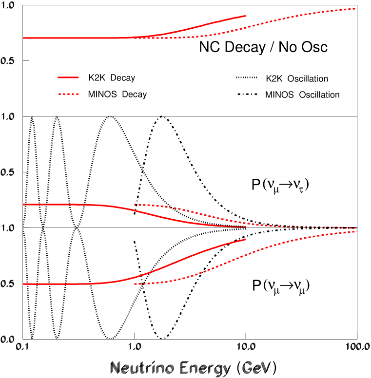
and determines the amount by which the predicted neutral-current rates are affected compared to the no oscillations (or the $\nu_{\mu}$–$\nu_{\tau}$ oscillations) case. In Fig. 3 we give the results for $P(\nu_{\mu}\to\nu_{\mu})$, $P(\nu_{\mu}\to\nu_{\tau})$ and $P(\nu_{\mu}\to\nu_{\mu})+P(\nu_{\mu}\to\nu_{\tau})$ for the decay model and compare them to the $\nu_{\mu}$–$\nu_{\tau}$ oscillations, for both the K2Kwho and MINOSminos (or the corresponding European projectNGS ) long-baseline experiments, with the oscillation and decay parameters as determined in the fits above.

The K2K experiment, already underway, has a low energy beam $E_{\nu}\approx 1\mbox{--}2$ GeV and a baseline $L=250$ km. The MINOS experiment will have 3 different beams, with average energies $E_{\nu}=3,$ 6 and 12 GeV and a baseline $L=732$ km. The approximate $L/E_{\nu}$ ranges are thus 125–250 km/GeV for K2K and 50–250 km/GeV for MINOS. The comparisons in Figure 3 show that the energy dependence of $\nu_{\mu}$ survival probability and the neutral current rate can both distinguish between the decay and the oscillation models. MINOS and the European project may also have $\tau$ detection capabilities that would allow additional tests.

Big Bang Nucleosynthesis

The decay of $\nu_{2}$ is sufficiently fast that all the neutrinos ($\nu_{e},\nu_{\mu},\nu_{\tau},\nu_{s}$) and the Majoron may be expected to equilibrate in the early universe before the primordial neutrinos decouple. When they achieve thermal equilibrium each Majorana neutrino contributes $N_{\nu}=1$ and the Majoron contributes $N_{\nu}=4/7$ kolb , giving and effective number of light neutrinos $N_{\nu}=4{4\over 7}$ at the time of Big Bang Nucleosynthesis. From the observed primordial abundances of ⁴He and ⁶Li, upper limits on $N_{\nu}$ are inferred, but these depend on which data are usedolive ; lisi ; burles . Conservatively, the upper limit to $N_{\nu}$ could extend up to 5.3 (or even to 6 if ⁷Li is depleted in halo starsolive ).

Cosmic Neutrino Fluxes

Since we expect both $\nu_{2}$ and $\nu_{3}$ to decay, neutrino beams from distant sources (such as Supernovae, active galactic nuclei and gamma-ray bursters) should contain only $\nu_{e}$ and $\bar{\nu}_{e}$ but no $\nu_{\mu}$, $\bar{\nu}_{\mu}$, $\nu_{\tau}$ and $\bar{\nu}_{\tau}$. This is a very strong prediction of our decay scenario. We can compare the very different expectations for neutrino flavor mixes from very distant sources such as AGN’s or GRB’s. Let us suppose that at the source the flux ratios are typical of a beam dump, a reasonable assumption: $N_{\nu_{e}}:N_{\nu_{\mu}}:N_{\nu_{\tau}}=1:2:0$. Then, for the conventional oscillation scenario, when all the $\delta m^{2}$’s satisfy $\delta m^{2}\ L/4E>>1$, it turns out curiously enough that for a wide variety of choices of neutrino mixing matrices, the final flavor mix is the same, namely: $N_{\nu_{e}}:N_{\nu_{\mu}}:N_{\nu_{\tau}}=1:1:1$. In the case of the decay B scenario, as mentioned here, we have $N_{\nu_{e}}:N_{\nu_{\mu}}:N_{\nu_{\tau}}=1:0:0.$ The two are quite distinct. Techniques for determining these flavor mixes in future KM3 neutrino telescopes have been proposedlearned .

Reactor and Accelerator Limits

The $\nu_{e}$ is essentially decoupled from the decay state $\nu_{2}$ so the null observations from the CHOOZ reactor are satisfiedchooz . The mixings of $\nu_{\mu}$ and $\nu_{\tau}$ with $\nu_{s}$ and $\nu_{e}$ are very small, so there is no conflict with stringent accelerator limits on flavor oscillations with large $\delta m^{2}$ zuber .

Summary

In summary, neutrino decay remains a viable alternative to neutrino oscillations as an explanation of the atmospheric neutrino anomaly. The model consists of two nearly degenerate mass eigenstates $\nu_{2}$, $\nu_{3}$ with mass separation $\stackrel{{\scriptstyle\sim}}{{>}}{\cal O}(25$ eV) from another nearly degenerate pair $\nu_{1}$, $\nu_{4}$. The $\nu_{\mu}$ and $\nu_{\tau}$ flavors are approximately composed of $\nu_{2}$ and $\nu_{3}$, with a mixing angle $\theta_{23}\simeq 57^{\circ}$. The state $\nu_{2}$ is unstable, decaying to $\bar{\nu}_{4}$ and a Majoron with a lifetime $\tau_{2}\sim 10^{-12}$ sec. The electron neutrino $\nu_{e}$ and a sterile neutrino $\nu_{s}$ have negligible mixing with $\nu_{\mu},\nu_{\tau}$ and are approximate mass eigenstates ($\nu_{e}\approx\nu_{1},\nu_{s}\approx\nu_{4})$, with a small mixing angle $\theta_{14}$ and a $\delta m_{41}^{2}\approx 10^{-5}\rm\,eV^{2}$ to explain the solar neutrino anomaly. The states $\nu_{3}$ and $\nu_{4}$ are also unstable, but with $\nu_{3}$ lifetime somewhat longer and $\nu_{4}$ lifetime much longer than the $\nu_{2}$ lifetime. This decay scenario is difficult to distinguish from oscillations because of the smearing in both L and $E_{\nu}$ in atmospheric neutrino events. However, long-baseline experiments, where $L$ is fixed, should be able to establish whether the dependence of $L/E_{\nu}$ is exponential or sinusoidal. In this scenario only $\nu_{1}$ is stable. Thus, neutrinos of supernovae or of extra galactic origin would be almost entirely $\nu_{e}$. The contribution of the electron neutrinos and the Majorons to the cosmological energy density $\Omega$ is negligible and not relevant for large scale structure formation.

VII Conclusion

In general, when neutrinos have masses and do mix; they can decay as well as oscillate. Some neutrino anomalies may be caused by one or the other or both. Non-oscillatory explanations have to be ruled out experimentally. Eventually, invisible neutrino decays can be severely constrained when data from Long Baseline experiments with good resolution in L and E become available.

Figure 1: Comparison of decay model (solid histograms) and $\nu_{\mu}$–$\nu_{\tau}$ oscillation model (dashed histograms) with SuperK data.

Figure 2: Survival probabiliity for $\nu_{\mu}$ versus $\log_{10}(L/E)$ for the decay model (heavy solid curve) and $\nu_{\mu}$ oscillation model (thin curve).

Figure 3: Long-baseline expectations for the K2K and MINOS long-baseline experiments from the decay model and the $\nu_{\mu}$–$\nu_{\tau}$ oscillation model. The upper panel gives the neutral current predictions compared to no oscillations (or $\nu_{\mu}$–$\nu_{\tau}$ oscillations).

References

- (1) V. Barger, these proceedings.
- (2) M. Kawasaki, K. Kohri and K. Sato, Phys. Lett. B340, 132 (1998); R. A. Malaney and G. Starkman, Phys. Rev. D52, 5480 (1995); A. Dolgov, S. Pastore and J. Valle, astro-ph-950611.
- (3) S. Petcov, Sov. J. Nucl. Phys. 24, 340 (1977), ibid. 25, 698 (1977); W. Marciano and A. Sanda, Phys. Lett. B67, 303 (1977).
- (4) J. Nieves and P. Pal, Phys. Rev. D40, 1693 (1989); J.C. D’Olivo, J. Nieves and P. Pal, Phys. Rev. D40, 3679 (1989).
- (5) C. Caso et al, Review of Particle Properties, Particle Data Group,Eur. Phys. J. C3, 1 (1998).
- (6) J-M. Frere, R.B. Nevzorov and M. Vysotsky, Phys. Lett. B394, 127 (1997).
- (7) D. Sciama, Ap. J. 364, 549 (1990); Phys. Rev. Lett. 65, 2839 (1990); Nature 348, (1990); D. Sciama, P. Salacci and M. Persic, Nature 358, 718 (1992). D. Sciama, Ap. J. 409, L25 (1993); D. Sciama, SISSA-61-98-A (June 1998).
- (8) R.N. Mohapatra and D. Sciama, hep-ph/9811446.
- (9) S. Bowyer et al., astro-ph/9906241.
- (10) B.W. Lee and R. Shrock, Phys. Rev. D16, 1444 (1977); S.T. Petcov, Phys. Lett. B68, 365 (1977); W. Marciano and A.I. Sanda, Phys. Lett. B67, 303 (1977).
- (11) M. Bilenky and A. Santamaria, hep-ph/9908272.
- (12) A. Jodidio et al, Phys. Rev. D34, 1967 (1986).
- (13) G. Gelmini and M. Roncadelli, Phys. Lett. B99, 411 (1981).
- (14) Y. Chikasige, R. Mohapatra and R. Peccei, Phys. Rev. Lett. 45, 1926 (1980).
- (15) J. Valle, Phys. Lett. B131, 87 (1983); G. Gelmini and J. Valle, ibid B142, 181 (1983), A. Choi and A. Santamaria, Phys. Lett. B267, 504 (1991); A. Joshipura and S. Rindani, Phys. Rev. D4, 300 (1992).
- (16) V. Barger, W-Y. Keung and S. Pakvasa, Phys. Rev. D25, 907 (1982).
- (17) S. Pakvasa and K. Tennakone, Phys. Rev. Lett. 28, 1415 (1972); J.N. Bahcall, N. Cabibbo and A. Yahil, Phys. Rev. Lett. 28, 316 (1972); See also A. Acker, A. Joshipura and S. Pakvasa, Phys. Lett. B285, 371 (1992); Z. Berezhiani, G. Fiorentini, A. Rossi and M. Moretti, JETP Lett. 55, 151 (1992).
- (18) A. Acker and S. Pakvasa (in preparation); A. Acker and S. Pakvasa, Phys. Lett. B320, 320 (1994).
- (19) P.F. Harrison, D.H. Perkins and W.G. Scott, Phys. Lett. B428, 79(1999); A. Acker, J.G. Learned, S. Pakvasa and T.J. Weiler, Phys. Lett. B298, 149 (1993); G. Conforto, M. Barone and C. Grimani, Phys. Lett. B447, 122 (1999); A. Strumia, JHEP 9904, 026 (1999).
- (20) V. Barger, J. G. Learned, S. Pakvasa and T.J. Weiler, Phys. Rev. Lett. 82, 2640 (1999).
- (21) P. Lipari and M. Lusignoli, Phys. Rev. D60, 013003 (1999); G. L. Fogli, E. Lisi and A. Marrone, Phys. Rev. D59, 117303 (1999); S. Choubey and S. Goswami, hep/ph-9904257.
- (22) V. Barger, J. G. Learned, P. Lipari, M. Lusignoli, S. Pakvasa and T. J. Weiler, Phys. Lett. B462, 109 (1999).
- (23) Y. Fukuda et al.(the Super-Kamiokande Collaboration), Phys. Rev. Lett. 81, 1562 (1998); ibid 82, 2644 (1998) ; T. Kajita hep-ex/9810001. The use of more recent data (K. Scholberg, hep-ex/9905016) does not change the conclusions.
- (24) A. Joshipura (private communication).
- (25) T. Kajita, Super-Kamiokande results presented at the “Beyond the Desert” Workshop, Castle Ringberg, Tegernsee, Germany, June 6–12, 1999 (to be published in the proceedings).
- (26) V. Barger, N. Deshpande, P. Pal, R.J.N. Phillips and K. Whisnant, Phys. Rev. D43, 1759 (1991); E. Akhmedov, P. Lipari and M. Lusignoli, Phys. Lett. B300, 128 (1993).
- (27) J. Pantaleone, Phys. Rev. D49, 2152 (1994).
- (28) Q. Liu and A. Smirnov, Nucl. Phys. B524, 505 (1998); P. Lipari and M. Lusignoli, Phys. Rev. D58, 073005 (1998).
- (29) F. Vissani and A. Smirnov, Phys. Lett. B432, 376 (1998); J. Learned, S. Pakvasa, and J. Stone, Phys. Lett. B435, 131 (1998); L. Hall and H. Murayama, Phys. Lett. B436, 323 (1998).
- (30) KEK-PS E362, INS-924 report (1992).
- (31) MINOS Collaboration, NuMI-L-375 report (1998).
- (32) ICANOE, F. Emeudo et al., INFN-AE-99-07.
- (33) R. Kolb and M. S. Turner, The Early Universe, Addison - Wesley (1990).
- (34) K. Olive and D. Thomas, hep-ph/9811444.
- (35) E. Lisi, S. Sarkar and F. Villante, Phys. Rev. D59, 123520 (1999).
- (36) S. Burles, K. Nollett, J. Truran and M. S. Turner, Phys. Rev. Lett. 82, 4176 (1999).
- (37) J. G. Learned and S. Pakvasa, Astropart. Phys. 3, 267 (1995); F. Halzen and D. Saltzberg, Phys. Rev. Lett. 81, 5722 (1998).
- (38) M. Apollonio et al. (the CHOOZ Collaboration), Phys. Lett. B420, 320 (1998).
- (39) For a review of accelerator limits, see K. Zuber, Phys. Rep. 305, 295 (1998).