On the Applicability of Weak-Coupling Results in High Density QCD

Abstract

Quark matter at asymptotically high baryon chemical potential is in a color superconducting state characterized by a gap $\Delta$. We demonstrate that although present weak-coupling calculations of $\Delta$ are formally correct for $\mu\rightarrow\infty$, the contributions which have to this point been neglected are large enough that present results can only be trusted for $\mu\gg\mu_{c}\sim 10^{8}$ MeV. We make this argument by using the gauge dependence of the present calculation as a diagnostic tool. It is known that the present calculation yields a gauge invariant result for $\mu\rightarrow\infty$; we show, however, that the gauge dependence of this result only begins to decrease for $\mu\gtrsim\mu_{c}$, and conclude that the result can certainly not be trusted for $\mu<\mu_{c}$. In an appendix, we set up the calculation of the influence of the Meissner effect on the magnitude of the gap. This contribution to $\Delta$ is, however, much smaller than the neglected contributions whose absence we detect via the resulting gauge dependence.

I Introduction

The starting point for a description of matter at high baryon density and low temperature is a Fermi sea of quarks. The important degrees of freedom — those whose fluctuations cost little free energy — are those involving quarks near the Fermi surface. We know from the work of Bardeen, Cooper, and Schrieffer [1] that any attractive interaction between the quarks, regardless how weak, makes the Fermi sea unstable to the formation of a condensate of Cooper pairs. In QCD, the interaction of two quarks whose colors are antisymmetric (the color $\bar{\bf 3}_{A}$ channel) is attractive. (The attractiveness of this interaction can be seen from single-gluon exchange, as is relevant at short distances, or via counting strings or analyzing the instanton induced coupling, as may be relevant at longer distances.) We therefore expect that under any circumstance in which cold dense quark matter is present, it will be in a color superconducting phase [2, 3, 4, 5, 6]. The one caveat is that this conclusion is known to be false if the number of colors is $N_{c}=\infty$[7]. Recent work [8, 9] indicates that quark matter is in a color superconducting phase for $N_{c}$ less than of order thousands, and in this paper we only discuss QCD with $N_{c}=3$.

We now know much about the symmetries and physical properties of color superconducting quark matter. The dominant condensate in QCD with two flavors of quarks is in the color $\bar{\bf 3}_{A}$ channel, breaking $SU(3)_{\rm color}\rightarrow SU(2)$, and is a flavor singlet[2, 3, 4, 5, 6]. Quarks with two of three colors have a gap in this 2SC phase, and five of eight gluons get a mass via the Meissner effect. In QCD with three flavors of quarks, the Cooper pairs cannot be flavor singlets, and flavor symmetries are necessarily broken. The symmetries of the phase which results have been analyzed in Ref. [10], and were in fact first analyzed in a different (zero density) context in Ref. [11]. The dominant condensate locks color and flavor symmetries, leaving an unbroken global symmetry under simultaneous $SU(3)$ transformations of color, left-flavor, and right-flavor. In this CFL phase, all nine quarks have a gap and all eight gluons have a mass[10]. Chiral symmetry is spontaneously broken, as is baryon number, and there are consequently nine massless Goldstone bosons [10]. Matter in the CFL phase is therefore similar in many respects to superfluid hypernuclear matter [10, 12, 13, 14]. The fact that color superconducting phases always feature either chiral symmetry breaking (as in the CFL phase) or some quarks which remain gapless (as in the 2SC phase) may be understood as a consequence of imposing ’t Hooft’s anomaly matching criterion [15]. The first order phase transition between the CFL and 2SC phases has been analyzed in detail[13, 14, 16], but all that will concern us below is that any finite strange quark mass is unimportant at large enough $\mu$, and quark matter is therefore in the CFL phase at asymptotically large $\mu$.

Much recent work has resulted in two classes of estimates of the magnitude of $\Delta$, the gap in the density of quasiparticle states in the superconducting phase. The first class of estimates are done within the context of models whose parameters are chosen to give reasonable vacuum physics. Examples include analyses in which the interaction between quarks is replaced simply by four-fermion interactions with the quantum numbers of the instanton interaction[5, 6, 17] or of single-gluon exchange[10, 13] and more sophisticated analyses done using instanton liquid models[18, 19]. Renormalization group analyses have also been used to explore the space of all possible four-fermion interactions allowed by the symmetries of QCD[20, 21]. These methods yield results which are in qualitative agreement: the gaps range from several tens of MeV up to as much as about 100 MeV and the corresponding critical temperatures, above which the superconducting condensates vanish, can be as large as about 50 MeV.

The second class of estimates uses $\mu\rightarrow\infty$ physics as a guide. At asymptotically large $\mu$, models with short range interactions are bound to fail, because the dominant interaction is due to the long-range magnetic interaction coming from single-gluon exchange[22, 23]. The collinear infrared divergence in small-angle scattering via single-gluon exchange results in a gap which is parametrically larger at $\mu\rightarrow\infty$ than it would be for any point-like four-fermion interaction[3]. Son showed [23] that this collinear divergence is regulated by Landau damping (dynamical screening) and that as a consequence, the parametric dependence of the gap in the limit in which the QCD coupling $g\rightarrow 0$ is

$$\frac{\Delta}{\mu}\sim\frac{1}{g^{5}}\exp\left(-\,\frac{3\pi^{2}}{\sqrt{2}g}\right)\ ,$$ (1)

which is more easily seen as an expansion in $g$ when rewritten as

$$\ln\left(\frac{\Delta}{\mu}\right)=-\frac{3\pi^{2}}{\sqrt{2}}\frac{1}{g}-5\ln g+f(g)\ .$$ (2)

This equation should be viewed as a definition of $f(g)$, which will include a term which is constant for $g\rightarrow 0$ and terms which vanish for $g\rightarrow 0$. The result (1) has been confirmed using a variety of methods[24, 25, 26, 27, 28, 29], and several estimates of $\lim_{g\rightarrow 0}f(g)$ exist in the literature. For example, Schaefer and Wilczek find[24, 30]

$$\lim_{g\rightarrow 0}f(g)\sim\ln\left[2^{-1/3}256\pi^{4}\left(\frac{2}{3}\right)^{5/2}\right]=8.88$$ (3)

in the CFL phase (see also Ref. [25]), and Brown, Liu, and Ren[28] find a result for $\lim_{g\rightarrow 0}f(g)$ which is smaller by $(\pi^{2}+4)/8-\ln 2=1.04$. If this asymptotic expression is applied by taking $g=g(\mu)$ from the perturbative QCD $\beta$-function (with $\Lambda_{\rm QCD}=200$ MeV), evaluating $\Delta$ at $\mu\sim 500$ MeV yields gaps in rough agreement with the estimates based on zero-density phenomenology.

The central purpose of this paper is to demonstrate that this nice agreement must at present be seen as coincidental, because present estimates for $f$ are demonstrably uncontrolled for $g>g_{c}\sim 0.8$, corresponding to $\mu<\mu_{c}$ with $\mu_{c}\sim 10^{8}$ or higher.

The weak-coupling calculations are derived from analyses (done using varying approximations) of the one-loop Schwinger-Dyson equation without vertex correction, and (with one exception) yield gauge dependent results. However, Schaefer and Wilczek argue that the result for $\lim_{g\rightarrow 0}f(g)$ in such a calculation is gauge invariant. The one calculation which is gauge invariant throughout is the calculation of $T_{c}$ (and hence $\Delta$ since the BCS relation $T_{c}=0.57\Delta$ holds [25]) done by Brown, Liu, and Ren[28]. As in other calculations, however, these authors neglect vertex corrections. Our purpose is to use the fact that our calculation (like most) is gauge dependent, and only gauge invariant for $g\rightarrow 0$, to estimate the $g$ above which vertex corrections, left out of all calculations, cannot be neglected.

We begin by sketching the derivation of the one-loop Schwinger-Dyson equation for $\Delta$, making as few approximations as we can. We solve the resulting gap equation numerically in several different gauges. Our results are (yet one more) confirmation of (1). Furthermore, we do find evidence that the gauge dependence of $f$ decreases for $g\rightarrow 0$. However, this decrease only begins to set in for $g\lesssim 0.8$. This implies that the contributions to $\Delta$ which have been neglected — like those arising from vertex corrections — only become subleading for $g\ll g_{c}\sim 0.8$. If we translate $g_{c}$ to $\mu_{c}$ by assuming $g$ should be taken as $g(\mu)$, this corresponds to $\mu_{c}\sim 10^{8}$ MeV. Recent work [31] shows that $g$ should be evaluated at a much lower ($g$-dependent) scale than $\mu$. This means that the condition $g<g_{c}\sim 0.8$ would translate into $\mu>\mu_{c}$ with $\mu_{c}$ orders of magnitude larger than $\mu_{c}\sim 10^{8}$ MeV.

The original purpose of our investigation was to do a self-consistent calculation of the influence of the Meissner effect on the magnitude of the gap in the CFL phase. In the presence of a condensate, the gluon propagator is modified: some gluons get a mass. In the CFL phase, all gluons get a mass, and this makes a calculation based on perturbative single-gluon exchange a self-consistent and complete description of the physics at asymptotically large $\mu$, with no remaining infrared problems. (In the 2SC phase, in contrast, the calculation of $\Delta$ leaves unanswered any questions about the non-Abelian infrared physics of the three gluons left unscreened by the condensate.) We felt that this motivation warranted a self-consistent calculation in which we calculate the gap using a Schwinger-Dyson equation in which the gluon propagator is modified not only by the presence of the Fermi sea (Debye mass, Landau damping) but is also affected by the condensate (the Meissner effect). We set this calculation up in an appendix. Previous work, beginning with that of Ref. [23], shows that the form of Eq. (1) is unmodified by including the Meissner effect, but $f(g)$ is affected. Our preliminary results suggest that the changes in $f(g)$ are small, as anticipated in Refs. [23, 24, 27, 29, 32, 33]. Indeed, the effects of physics left out of the present analysis, which we have diagnosed via the gauge dependence of $f(g)$, are much larger than those introduced by the Meissner effect at any $g$ we have investigated.

II Deriving the gap equation

In this section, we derive the gap equation for QCD with three massless flavors which is valid at asymptotically high densities. We follow Ref. [24], but make fewer approximations. Because our point is to stress the importance of effects which we do not calculate, we will make our assumptions and approximations very clear as we proceed. In other words, since the lesson we learn from our results is that they cannot yet be trusted, it is important to detail carefully all points at which we leave something out.

We use the standard Nambu-Gorkov formalism by defining an eight-component field $\Psi=(\psi,\bar{\psi}^{T})$. In this basis, the inverse quark propagator takes the form

$$S^{-1}(k)=\left(\begin{array}[]{cc}k\!\!\!/+\mu\gamma_{0}&\bar{\Delta}\\ \Delta&(k\!\!\!/-\mu\gamma_{0})^{T}\end{array}\right)$$ (4)

where $\bar{\Delta}=\gamma_{0}\Delta^{\dagger}\gamma_{0}$. The color, flavor, and Dirac indices are suppressed in the above expression. The diagonal blocks correspond to ordinary propagation and the off-diagonal blocks reflect the possibility for “anomalous propagation” in the presence of a diquark condensate.

We make the following ansatz for the form of the gap matrix[4, 10, 24, 34]:

$$\Delta^{ab}_{ij}(k) =(\lambda^{A}_{I})^{ab}(\lambda^{A}_{I})_{ij}C\gamma_{5}\left({\Delta_{1}^{A}}(k_{0})P_{+}(k)+{\Delta_{2}^{A}}(k_{0})P_{-}(k)\right)$$ (5)

$$+(\lambda^{S}_{J})^{ab}(\lambda^{S}_{J})_{ij}C\gamma_{5}\left({\Delta_{1}^{S}}(k_{0})P_{+}(k)+{\Delta_{2}^{S}}(k_{0})P_{-}(k)\right)$$ (6)

Here, $a,b=1,2,3$ are color indices, $i,j=1,2,3$ are flavor indices, $\lambda^{A}_{I}$ are antisymmetric $U(3)$ color or flavor matrices with $I=1,2,3$, and $\lambda^{S}_{J}$ are symmetric $U(3)$ color or flavor with $J=1,\ldots,6$, and the projection operators $P_{\pm}$ are defined as

$$P_{+}(k)={{1+\vec{\alpha}\cdot\hat{k}}\over 2}$$ (7)

$$P_{-}(k)={{1-\vec{\alpha}\cdot\hat{k}}\over 2}$$ (8)

with $\vec{\alpha}=\gamma_{0}\vec{\gamma}$.

By making this ansatz, we are making several assumptions:

• First, we have taken $\Delta_{1}^{A}$, $\Delta_{2}^{A}$, $\Delta_{1}^{S}$, and $\Delta_{2}^{S}$ to be functions of $k_{0}$ only. All are in principle functions of both $k_{0}$ and $|\vec{k}|$, but we assume that they are dominated by $|\vec{k}|\sim\mu$. This is a standard assumption, and although we do not expect that relaxing this assumption would resolve the problems which we diagnose below, this does belong on the list of potential cures.

• Second, we have explicitly separated the gaps which are antisymmetric $\bar{\bf 3}_{A}$ in color and flavor from those which are symmetric ${\bf 6}_{S}$ in color and flavor and, in both cases, we have assumed that the favored channel is the one in which color and flavor rotations are locked. The color and flavor structure of our ansatz is thus precisely that first explored in Ref. [10], which allows quarks of all three colors and all three flavors to pair. Subsequent work [30, 32, 33, 35] confirms that this is the favored condensate, and we will not attempt to further generalize it here.

• Third, we have assumed that the Cooper pairs in the condensate have zero spin and orbital angular momentum. This seems a safe assumption in the CFL phase, where the dominant condensate, made of Cooper pairs with zero spin and orbital angular momentum, leaves no quarks ungapped.

• Fourth, we neglect $\bar{\psi}\psi$ condensates. Since chiral symmetry is broken in the CFL phase, these must be nonzero [10]. This applies to both color singlet and color octet $\bar{\psi}\psi$ condensates[36]. Such condensates are small[19, 30], however, and we expect that neglecting them results in only a very small error in the magnitude of the dominant diquark condensate.

The most important assumption we make is that we obtain the gap by solving the one-loop Schwinger-Dyson equation of the form

$$S^{-1}(k)-S_{0}^{-1}(k)=ig^{2}\int\frac{d^{4}q}{(2\pi)^{4}}\Gamma_{\mu}^{a}S(q)\Gamma_{\nu}^{b}D_{ab}^{\mu\nu}(k-q)\ ,$$ (9)

using a medium-modified gluon propagator described below and unmodified vertices

$$\Gamma_{\mu}^{a}=\left(\begin{array}[]{cc}\gamma_{\mu}\lambda^{a}/2&0\\ 0&-(\gamma_{\mu}\lambda^{a}/2)^{T}\end{array}\right).$$ (10)

Here, $S_{0}$ is the bare fermion propagator with $\Delta=0$. Note that we use a Minkowski metric unless stated otherwise. We will demonstrate that our results are completely uncontrolled for $g>g_{c}\sim 0.8$. This breakdown could in principle reflect a failure of any of our assumptions. We expect, however, that it arises because contributions which have been truncated in writing (9) are large for $g>g_{c}$. That is, we expect that this truncation (and not any of the simplifications introduced by our ansatz for $\Delta$) is the most significant assumption we are making.

We obtain four coupled gap equations

$$\Delta^{A}_{1,2}(k_{0})=-{i\over 6}g^{2}\int\frac{d^{4}q}{(2\pi)^{4}}{\rm Tr}\left[P_{\pm}(k)\gamma_{\mu}\left(P_{+}(q)a_{+}(q)+P_{-}(q)a_{-}(q)\right)\gamma_{\nu}\right]D^{\mu\nu}(k-q)$$ (11)

$$\Delta^{S}_{1,2}(k_{0})=-{i\over 6}g^{2}\int\frac{d^{4}q}{(2\pi)^{4}}{\rm Tr}\left[P_{\pm}(k)\gamma_{\mu}\left(P_{+}(q)b_{+}(q)+P_{-}(q)b_{-}(q)\right)\gamma_{\nu}\right]D^{\mu\nu}(k-q)$$ (12)

where $P_{\pm}$ means $P_{+}$ in the $\Delta_{1}$ equation and $P_{-}$ in the $\Delta_{2}$ equation and where

$$a_{+}(q) = {-{\Delta_{2}^{S}}(q_{0})-{\Delta_{2}^{A}}(q_{0})\over q_{0}^{2}-(|\vec{q}|+\mu)^{2}-4\left[{\Delta_{2}^{A}}(q_{0})+2{\Delta_{2}^{S}}(q_{0})\right]^{2}}$$ (13)

$$+{\left[{\Delta_{2}^{A}}(q_{0})-{\Delta_{2}^{S}}(q_{0})\right]\left[-q_{0}^{2}+(|\vec{q}|+\mu)^{2}+(5{\Delta_{2}^{A}}(q_{0})+7{\Delta_{2}^{S}}(q_{0}))({\Delta_{2}^{A}}(q_{0})+3{\Delta_{2}^{S}}(q_{0}))\right]\over\left[q_{0}^{2}-(|\vec{q}|+\mu)^{2}-({\Delta_{2}^{A}}(q_{0})-{\Delta_{2}^{S}}(q_{0}))^{2}\right]\left[q_{0}^{2}-(|\vec{q}|+\mu)^{2}-4({\Delta_{2}^{A}}(q_{0})+2{\Delta_{2}^{S}}(q_{0}))^{2}\right]}$$ (14)

$$a_{-}(q) = {-{\Delta_{1}^{S}}(q_{0})-{\Delta_{1}^{A}}(q_{0})\over q_{0}^{2}-(|\vec{q}|-\mu)^{2}-4\left[{\Delta_{1}^{A}}(q_{0})+2{\Delta_{1}^{S}}(q_{0})\right]^{2}}$$ (15)

$$+{\left[{\Delta_{1}^{A}}(q_{0})-{\Delta_{1}^{S}}(q_{0})\right]\left[-q_{0}^{2}+(|\vec{q}|-\mu)^{2}+(5{\Delta_{1}^{A}}(q_{0})+7{\Delta_{1}^{S}}(q_{0}))({\Delta_{1}^{A}}(q_{0})+3{\Delta_{1}^{S}}(q_{0}))\right]\over\left[q_{0}^{2}-(|\vec{q}|-\mu)^{2}-({\Delta_{1}^{A}}(q_{0})-{\Delta_{1}^{S}}(q_{0}))^{2}\right]\left[q_{0}^{2}-(|\vec{q}|-\mu)^{2}-4({\Delta_{1}^{A}}(q_{0})+2{\Delta_{1}^{S}}(q_{0}))^{2}\right]}$$ (16)

$$b_{+}(q) = {{\Delta_{2}^{S}}(q_{0})\over q_{0}^{2}-(|\vec{q}|+\mu)^{2}-4\left[{\Delta_{2}^{A}}(q_{0})+2{\Delta_{2}^{S}}(q_{0})\right]^{2}}$$ (17)

$$+{\left[{\Delta_{2}^{A}}(q_{0})-{\Delta_{2}^{S}}(q_{0})\right]\left[{\Delta_{2}^{A}}(q_{0})+{\Delta_{2}^{S}}(q_{0})\right]\left[{\Delta_{2}^{A}}(q_{0})+5{\Delta_{2}^{S}}(q_{0})\right]\over\left[q_{0}^{2}-(|\vec{q}|+\mu)^{2}-({\Delta_{2}^{A}}(q_{0})-{\Delta_{2}^{S}}(q_{0}))^{2}\right]\left[q_{0}^{2}-(|\vec{q}|+\mu)^{2}-4({\Delta_{2}^{A}}(q_{0})+2{\Delta_{2}^{S}}(q_{0}))^{2}\right]}$$ (18)

$$b_{-}(q) = {{\Delta_{1}^{S}}(q_{0})\over q_{0}^{2}-(|\vec{q}|-\mu)^{2}-4\left[{\Delta_{1}^{A}}(q_{0})+2{\Delta_{1}^{S}}(q_{0})\right]^{2}}$$ (19)

$$+{\left[{\Delta_{1}^{A}}(q_{0})-{\Delta_{1}^{S}}(q_{0})\right]\left[{\Delta_{1}^{A}}(q_{0})+{\Delta_{1}^{S}}(q_{0})\right]\left[{\Delta_{1}^{A}}(q_{0})+5{\Delta_{1}^{S}}(q_{0})\right]\over\left[q_{0}^{2}-(|\vec{q}|-\mu)^{2}-({\Delta_{1}^{A}}(q_{0})-{\Delta_{1}^{S}}(q_{0}))^{2}\right]\left[q_{0}^{2}-(|\vec{q}|-\mu)^{2}-4({\Delta_{1}^{A}}(q_{0})+2{\Delta_{1}^{S}}(q_{0}))^{2}\right]}\ .$$ (20)

In a general covariant gauge, the resummed gluon propagator is given by

$$D_{\mu\nu}(q)={P^{T}_{\mu\nu}\over q^{2}-G(q)}+{P^{L}_{\mu\nu}\over q^{2}-F(q)}-\xi{q_{\mu}q_{\nu}\over q^{4}}$$ (21)

where $G(q)$ and $F(q)$ are functions of $q_{0}$ and $|\vec{q}|$ and the projectors $P^{T,L}_{\mu\nu}$ are defined as follows:

$$P^{T}_{ij}=\delta_{ij}-\hat{q_{i}}\hat{q_{j}},\ P^{T}_{00}=P^{T}_{0i}=0,\ P^{L}_{\mu\nu}=-g_{\mu\nu}+{q_{\mu}q_{\nu}\over q^{2}}-P^{T}_{\mu\nu}.$$ (22)

The functions $F$ and $G$ describe the effects of the medium on the gluon propagator. If we neglect the Meissner effect (that is, if we neglect the modification of $F(q)$ and $G(q)$ due to the gap $\Delta$ in the fermion propagator) then $F(q)$ describes Thomas-Fermi screening and $G(q)$ describes Landau damping and they are given in the HDL approximation by[37]

$$F(q) = m^{2}{q^{2}\over|\vec{q}|}\left(1-{iq_{0}\over|\vec{q}|}Q_{0}\left({iq_{0}\over|\vec{q}|}\right)\right),\ \ \ \ \ \ {\rm with}\ Q_{0}(x)={1\over 2}\log\left({x+1\over x-1}\right)$$ (23)

$$G(q) = {1\over 2}m^{2}{iq_{0}\over|\vec{q}|}\left[\left(1-\left({iq_{0}\over|\vec{q}|}\right)^{2}\right)Q_{0}\left({iq_{0}\over|\vec{q}|}\right)+{iq_{0}\over|\vec{q}|}\right]\ ,$$ (24)

where $m^{2}=3g^{2}\mu^{2}/2\pi^{2}$ is the Debye screening mass for $N_{f}=3$. We discuss the modifications of $F(q)$ and $G(q)$ due to the Meissner effect in an Appendix.

In order to obtain the final form of the gap equation, we need the following trace:

$$\begin{array}[]{l}{\rm Tr}\left[P_{\pm}(k)\gamma_{\mu}\left(P_{+}(q)a_{+}(q)+P_{-}(q)a_{-}(q)\right)\gamma_{\nu}\right]D^{\mu\nu}(k-q)\\ \\ \begin{array}[]{lll}&=a_{+}(q)&\left[2{-1\mp\widehat{(k-q)}\cdot\hat{k}\widehat{(k-q)}\cdot\hat{q}\over(k-q)^{2}-G(k-q)}+{-1\mp\hat{k}\cdot\hat{q}{(k-q)_{0}^{2}+(\vec{k}-\vec{q})^{2}\over(k-q)^{2}}\pm 2\widehat{(k-q)}\cdot\hat{k}\widehat{(k-q)}\cdot\hat{q}{(k-q)_{0}^{2}\over(k-q)^{2}}\over(k-q)^{2}-F(k-q)}\right.\\ &&+\left.{\xi\over(k-q)^{2}}\left(1\mp\hat{k}\cdot\hat{q}{(k-q)_{0}^{2}+(\vec{k}-\vec{q})^{2}\over(k-q)^{2}}\pm 2\widehat{(k-q)}\cdot\hat{k}\widehat{(k-q)}\cdot\hat{q}{(\vec{k}-\vec{q})^{2}\over(k-q)^{2}}\right)\right.\Biggr{]}\\ \\ &+a_{-}(q)&\left[2{-1\pm\widehat{(k-q)}\cdot\hat{k}\widehat{(k-q)}\cdot\hat{q}\over(k-q)^{2}-G(k-q)}+{-1\pm\hat{k}\cdot\hat{q}{(k-q)_{0}^{2}+(\vec{k}-\vec{q})^{2}\over(k-q)^{2}}\mp 2\widehat{(k-q)}\cdot\hat{k}\widehat{(k-q)}\cdot\hat{q}{(k-q)_{0}^{2}\over(k-q)^{2}}\over(k-q)^{2}-F(k-q)}\right.\\ &&+\left.{\xi\over(k-q)^{2}}\left(1\pm\hat{k}\cdot\hat{q}{(k-q)_{0}^{2}+(\vec{k}-\vec{q})^{2}\over(k-q)^{2}}\mp 2\widehat{(k-q)}\cdot\hat{k}\widehat{(k-q)}\cdot\hat{q}{(\vec{k}-\vec{q})^{2}\over(k-q)^{2}}\right)\right.\Biggr{]}\ .\end{array}\end{array}$$ (25)

This allows us to recast Eq. (11) into the following form:

$$\begin{array}[]{ll}\Delta_{1}^{A}(k_{0})=-{i\over 6}g^{2}\begin{minipage}[l][0.5in][c]{7.22743pt}\par\vskip 0.0pt\vskip 8.5pt plus 3.0pt minus 4.0pt\hbox to469.75499pt{\hskip 0.0pt\hskip 0.0pt plus 1000.0pt$\displaystyle\int$\hskip 0.0pt plus 1000.0pt}\vskip 8.5pt plus 3.0pt minus 4.0pt\noindent\ignorespaces\end{minipage}\frac{d^{4}q}{(2\pi)^{4}}&\!\left[a_{+}(q)\!\left(\!2{-1-\widehat{(k-q)}\cdot\hat{k}\widehat{(k-q)}\cdot\hat{q}\over(k-q)^{2}-G(k-q)}\!+\!{-1-\hat{k}\cdot\hat{q}{(k-q)_{0}^{2}+(\vec{k}-\vec{q})^{2}\over(k-q)^{2}}+2\widehat{(k-q)}\cdot\hat{k}\widehat{(k-q)}\cdot\hat{q}{(k-q)_{0}^{2}\over(k-q)^{2}}\over(k-q)^{2}-F(k-q)}\right.\right.\\ &+\!\left.{\xi\over(k-q)^{2}}\!\left(\!1\!-\!\hat{k}\cdot\hat{q}{(k-q)_{0}^{2}+(\vec{k}-\vec{q})^{2}\over(k-q)^{2}}\!+\!2\widehat{(k-q)}\cdot\hat{k}\widehat{(k-q)}\cdot\hat{q}{(\vec{k}-\vec{q})^{2}\over(k-q)^{2}}\right)\right)\\ &+a_{-}(q)\!\!\left(\!2{-1+\widehat{(k-q)}\cdot\hat{k}\widehat{(k-q)}\cdot\hat{q}\over(k-q)^{2}-G(k-q)}\!+\!{-1+\hat{k}\cdot\hat{q}{(k-q)_{0}^{2}+(\vec{k}-\vec{q})^{2}\over(k-q)^{2}}-2\widehat{(k-q)}\cdot\hat{k}\widehat{(k-q)}\cdot\hat{q}{(k-q)_{0}^{2}\over(k-q)^{2}}\over(k-q)^{2}-F(k-q)}\right.\\ &+\!\left.\left.{\xi\over(k-q)^{2}}\!\left(\!1\!+\!\hat{k}\cdot\hat{q}{(k-q)_{0}^{2}+(\vec{k}-\vec{q})^{2}\over(k-q)^{2}}\!-\!2\widehat{(k-q)}\cdot\hat{k}\widehat{(k-q)}\cdot\hat{q}{(\vec{k}-\vec{q})^{2}\over(k-q)^{2}}\right)\right)\right]\\ &\\ \Delta_{2}^{A}(k_{0})=-{i\over 6}g^{2}\begin{minipage}[l][0.5in][c]{7.22743pt}\par\vskip 0.0pt\vskip 8.5pt plus 3.0pt minus 4.0pt\hbox to469.75499pt{\hskip 0.0pt\hskip 0.0pt plus 1000.0pt$\displaystyle\int$\hskip 0.0pt plus 1000.0pt}\vskip 8.5pt plus 3.0pt minus 4.0pt\noindent\ignorespaces\end{minipage}\frac{d^{4}q}{(2\pi)^{4}}&\!\left[a_{+}(q)\!\left(\!2{-1+\widehat{(k-q)}\cdot\hat{k}\widehat{(k-q)}\cdot\hat{q}\over(k-q)^{2}-G(k-q)}\!+\!{-1+\hat{k}\cdot\hat{q}{(k-q)_{0}^{2}+(\vec{k}-\vec{q})^{2}\over(k-q)^{2}}-2\widehat{(k-q)}\cdot\hat{k}\widehat{(k-q)}\cdot\hat{q}{(k-q)_{0}^{2}\over(k-q)^{2}}\over(k-q)^{2}-F(k-q)}\right.\right.\\ &+\!\left.{\xi\over(k-q)^{2}}\!\left(\!1\!+\!\hat{k}\cdot\hat{q}{(k-q)_{0}^{2}+(\vec{k}-\vec{q})^{2}\over(k-q)^{2}}\!-\!2\widehat{(k-q)}\cdot\hat{k}\widehat{(k-q)}\cdot\hat{q}{(\vec{k}-\vec{q})^{2}\over(k-q)^{2}}\right)\right)\\ &+a_{-}(q)\!\!\left(2{-1-\widehat{(k-q)}\cdot\hat{k}\widehat{(k-q)}\cdot\hat{q}\over(k-q)^{2}-G(k-q)}\!+\!{-1-\hat{k}\cdot\hat{q}{(k-q)_{0}^{2}+(\vec{k}-\vec{q})^{2}\over(k-q)^{2}}+2\widehat{(k-q)}\cdot\hat{k}\widehat{(k-q)}\cdot\hat{q}{(k-q)_{0}^{2}\over(k-q)^{2}}\over(k-q)^{2}-F(k-q)}\right.\\ &+\!\left.\left.{\xi\over(k-q)^{2}}\!\left(\!1\!-\!\hat{k}\cdot\hat{q}{(k-q)_{0}^{2}+(\vec{k}-\vec{q})^{2}\over(k-q)^{2}}\!+\!2\widehat{(k-q)}\cdot\hat{k}\widehat{(k-q)}\cdot\hat{q}{(\vec{k}-\vec{q})^{2}\over(k-q)^{2}}\right)\right)\right]\end{array}$$ (26)

$$\begin{array}[]{ll}\Delta_{1}^{S}(k_{0})=-{i\over 6}g^{2}\begin{minipage}[l][0.5in][c]{7.22743pt}\par\vskip 0.0pt\vskip 8.5pt plus 3.0pt minus 4.0pt\hbox to469.75499pt{\hskip 0.0pt\hskip 0.0pt plus 1000.0pt$\displaystyle\int$\hskip 0.0pt plus 1000.0pt}\vskip 8.5pt plus 3.0pt minus 4.0pt\noindent\ignorespaces\end{minipage}\frac{d^{4}q}{(2\pi)^{4}}&\!\left[b_{+}(q)\!\left(\!2{-1-\widehat{(k-q)}\cdot\hat{k}\widehat{(k-q)}\cdot\hat{q}\over(k-q)^{2}-G(k-q)}\!+\!{-1-\hat{k}\cdot\hat{q}{(k-q)_{0}^{2}+(\vec{k}-\vec{q})^{2}\over(k-q)^{2}}+2\widehat{(k-q)}\cdot\hat{k}\widehat{(k-q)}\cdot\hat{q}{(k-q)_{0}^{2}\over(k-q)^{2}}\over(k-q)^{2}-F(k-q)}\right.\right.\\ &+\!\left.{\xi\over(k-q)^{2}}\!\left(\!1\!-\!\hat{k}\cdot\hat{q}{(k-q)_{0}^{2}+(\vec{k}-\vec{q})^{2}\over(k-q)^{2}}\!+\!2\widehat{(k-q)}\cdot\hat{k}\widehat{(k-q)}\cdot\hat{q}{(\vec{k}-\vec{q})^{2}\over(k-q)^{2}}\right)\right)\\ &+b_{-}(q)\!\!\left(\!2{-1+\widehat{(k-q)}\cdot\hat{k}\widehat{(k-q)}\cdot\hat{q}\over(k-q)^{2}-G(k-q)}\!+\!{-1+\hat{k}\cdot\hat{q}{(k-q)_{0}^{2}+(\vec{k}-\vec{q})^{2}\over(k-q)^{2}}-2\widehat{(k-q)}\cdot\hat{k}\widehat{(k-q)}\cdot\hat{q}{(k-q)_{0}^{2}\over(k-q)^{2}}\over(k-q)^{2}-F(k-q)}\right.\\ &+\!\left.\left.{\xi\over(k-q)^{2}}\!\left(\!1\!+\!\hat{k}\cdot\hat{q}{(k-q)_{0}^{2}+(\vec{k}-\vec{q})^{2}\over(k-q)^{2}}\!-\!2\widehat{(k-q)}\cdot\hat{k}\widehat{(k-q)}\cdot\hat{q}{(\vec{k}-\vec{q})^{2}\over(k-q)^{2}}\right)\right)\right]\\ &\\ \Delta_{2}^{S}(k_{0})=-{i\over 6}g^{2}\begin{minipage}[l][0.5in][c]{7.22743pt}\par\vskip 0.0pt\vskip 8.5pt plus 3.0pt minus 4.0pt\hbox to469.75499pt{\hskip 0.0pt\hskip 0.0pt plus 1000.0pt$\displaystyle\int$\hskip 0.0pt plus 1000.0pt}\vskip 8.5pt plus 3.0pt minus 4.0pt\noindent\ignorespaces\end{minipage}\frac{d^{4}q}{(2\pi)^{4}}&\!\left[b_{+}(q)\!\left(\!2{-1+\widehat{(k-q)}\cdot\hat{k}\widehat{(k-q)}\cdot\hat{q}\over(k-q)^{2}-G(k-q)}\!+\!{-1+\hat{k}\cdot\hat{q}{(k-q)_{0}^{2}+(\vec{k}-\vec{q})^{2}\over(k-q)^{2}}-2\widehat{(k-q)}\cdot\hat{k}\widehat{(k-q)}\cdot\hat{q}{(k-q)_{0}^{2}\over(k-q)^{2}}\over(k-q)^{2}-F(k-q)}\right.\right.\\ &+\!\left.{\xi\over(k-q)^{2}}\!\left(\!1\!+\!\hat{k}\cdot\hat{q}{(k-q)_{0}^{2}+(\vec{k}-\vec{q})^{2}\over(k-q)^{2}}\!-\!2\widehat{(k-q)}\cdot\hat{k}\widehat{(k-q)}\cdot\hat{q}{(\vec{k}-\vec{q})^{2}\over(k-q)^{2}}\right)\right)\\ &+b_{-}(q)\!\!\left(2{-1-\widehat{(k-q)}\cdot\hat{k}\widehat{(k-q)}\cdot\hat{q}\over(k-q)^{2}-G(k-q)}\!+\!{-1-\hat{k}\cdot\hat{q}{(k-q)_{0}^{2}+(\vec{k}-\vec{q})^{2}\over(k-q)^{2}}+2\widehat{(k-q)}\cdot\hat{k}\widehat{(k-q)}\cdot\hat{q}{(k-q)_{0}^{2}\over(k-q)^{2}}\over(k-q)^{2}-F(k-q)}\right.\\ &+\!\left.\left.{\xi\over(k-q)^{2}}\!\left(\!1\!-\!\hat{k}\cdot\hat{q}{(k-q)_{0}^{2}+(\vec{k}-\vec{q})^{2}\over(k-q)^{2}}\!+\!2\widehat{(k-q)}\cdot\hat{k}\widehat{(k-q)}\cdot\hat{q}{(\vec{k}-\vec{q})^{2}\over(k-q)^{2}}\right)\right)\right].\end{array}$$ (26)

III Solving the gap equation

In order to obtain a tractable numerical problem, we make two further simplifying assumptions:

• First, at weak coupling we expect the physics to be dominated by particles and holes near the Fermi surface. This manifests itself in Eq. (26) in the fact that $a_{-}$ and $b_{-}$ have singularities on the Fermi surface while $a_{+}$ and $b_{+}$ are regular there, and we therefore expect that at weak coupling we can neglect $a_{+}$ and $b_{+}$. Upon doing this, we have equations for $\Delta_{1}^{A,S}$ which do not involve $\Delta_{2}^{A,S}$. We are only interested in $\Delta_{1}^{A,S}$, since $\Delta_{2}^{A,S}$ describe the propagation of antiparticles far from the Fermi surface. If we assume that we are at weak enough coupling that $a_{+}$ and $b_{+}$ can be neglected (that is if we assume that $\Delta_{1}^{A,S}\ll\mu$) then we can ignore $\Delta_{2}^{A,S}$ in our calculation of $\Delta_{1}^{A,S}$. (Note that we are not assuming that $\Delta_{2}^{A,S}$ is any smaller than $\Delta_{1}^{A,S}$; there is no reason for this to be true.) We will see that our results break down for $g\gtrsim 0.8$, at which $\Delta<10^{-7}\mu$. Because $\Delta\ll\mu$, neglecting the effects of $\Delta_{2}^{A,S}$ on $\Delta_{1}^{A,S}$ should be a good approximation, and we do not expect that including these effects would cure the problems we discover. This should, however, be investigated further.

• Second, we set $\Delta_{1}^{S}=0$, and solve an equation for $\Delta_{1}^{A}$ alone. This assumption is in fact inconsistent, as the gap in the symmetric channel must be nonzero. This is clear from explicit examination of the gap equations Eq. (26) (and indeed of the gap equations of Ref. [10]). In fact, this result is manifest on symmetry grounds [13, 38]: in the presence of $\Delta_{1}^{A}\neq 0$, a nonzero $\Delta_{1}^{S}$ breaks no new global symmetries and there is therefore no symmetry to keep it zero. Because single-gluon exchange is repulsive in the symmetric channel, this condensate can only exist in the presence of condensation in the antisymmetric channel. Explicit calculation [10, 30, 32] shows that the symmetric condensates are much smaller than those in the antisymmetric channels. We are therefore confident that keeping $\Delta_{1}^{S}$ would yield only a very small correction to $\Delta_{1}^{A}$.

We must now solve a single gap equation for $\Delta_{1}^{A}(k_{0})$, which henceforth we denote simply as $\Delta(k_{0})$. The reader will see below that this equation is still rather involved. Most authors have made further approximations, valid for $g\rightarrow 0$. Because we make no further approximations, our results cannot be gauge invariant. This allows us to test the claim that the results become gauge invariant in the limit $g\rightarrow 0$, and to use the rapidity of the disappearance of gauge dependence as this limit is approached to evaluate at what $g$ the contributions we have truncated can legitimately be ignored.

In order to obtain numerical solutions, it is convenient to do a Wick rotation $q_{0}\rightarrow iq_{0}$ to Euclidean space, yielding the gap equation

$$\Delta(k_{0}) = {g^{2}\over 6}\!\int\!\frac{d^{4}q}{(2\pi)^{4}}\Biggl{[}{\Delta(q_{0})\over q_{0}^{2}+(|\vec{q}|-\mu)^{2}+4\Delta^{2}(q_{0})}$$ (27)

$$\qquad\qquad+{\Delta(q_{0})\left(q_{0}^{2}+(|\vec{q}|-\mu)^{2}+5\Delta^{2}(q_{0})\right)\over\left(q_{0}^{2}+(|\vec{q}|-\mu)^{2}+\Delta^{2}(q_{0})\right)\left(q_{0}^{2}+(|\vec{q}|-\mu)^{2}+4\Delta^{2}(q_{0})\right)}\Biggr{]}$$ (28)

$$\qquad\Biggl{[}2{1-\widehat{(k-q)}\cdot\hat{k}\widehat{(k-q)}\cdot\hat{q}\over(k-q)_{0}^{2}+(\vec{k}-\vec{q})^{2}+G(k_{0}-q_{0},|\vec{k}-\vec{q}|)}$$ (29)

$$\qquad\qquad+{1+\hat{k}\cdot\hat{q}{-(k-q)_{0}^{2}+(\vec{k}-\vec{q})^{2}\over(k-q)_{0}^{2}+(\vec{k}-\vec{q})^{2}}+2\widehat{(k-q)}\cdot\hat{k}\widehat{(k-q)}\cdot\hat{q}{(k-q)_{0}^{2}\over(k-q)_{0}^{2}+(\vec{k}-\vec{q})^{2}}\over(k-q)_{0}^{2}+(\vec{k}-\vec{q})^{2}+F(k_{0}-q_{0},|\vec{k}-\vec{q}|)}$$ (30)

$$\qquad\qquad+\xi{-1+\hat{k}\cdot\hat{q}{-(k-q)_{0}^{2}+(\vec{k}-\vec{q})^{2}\over(k-q)_{0}^{2}+(\vec{k}-\vec{q})^{2}}-2\widehat{(k-q)}\cdot\hat{k}\widehat{(k-q)}\cdot\hat{q}{(\vec{k}-\vec{q})^{2}\over(k-q)_{0}^{2}+(\vec{k}-\vec{q})^{2}}\over(k-q)_{0}^{2}+(\vec{k}-\vec{q})^{2}}\Biggr{]}.$$ (31)

The integral over the azimuthal angle $\phi$ is trivial, and we therefore have three integrals to do. We do the remaining angular integral analytically, after making a change of variables. We define

$\displaystyle\vec{q^{\prime}}=\vec{k}-\vec{q}$because the integration over the polar angle $\theta$ is simpler when the momentum integration is done over $\vec{q^{\prime}}$. The simplification arises because there is no longer any angular dependence in the functions $F$ and $G$:

$$F(k_{0}-q_{0},|\vec{k}-\vec{q}|)=F(k_{0}-q_{0},|\vec{q^{\prime}}|)$$

and similarly for $G$. After doing the angular integral, the gap equation reduces to a double integral equation with integration variables $|\vec{q^{\prime}}|$ (which we henceforth denote $q$) and $q_{0}$:

$$\Delta(k_{0}) = {g^{2}\over 48\pi^{3}}\int_{-\infty}^{\infty}dq_{0}\int_{0}^{\infty}dq\left[{\Delta(q_{0})\over(k_{0}-q_{0})^{2}+q^{2}+G(k_{0}-q_{0},q)}I_{G}(q_{0},q)\right.$$ (32)

$$\qquad\left.+{\Delta(q_{0})\over(k_{0}-q_{0})^{2}+q^{2}+F(k_{0}-q_{0},q)}I_{F}(k_{0},q_{0},q)+\xi{q\Delta(q_{0})\over(k_{0}-q_{0})^{2}+q^{2}}I_{\xi}(k_{0},q_{0},q)\right]$$ (33)

$${\rm where}$$ (34)

$$I_{G}(q_{0},q<\mu) = {2(q_{0}^{2}+4\Delta^{2}(q_{0})+q^{2})(q^{2}+4\mu^{2}-q_{0}^{2}-4\Delta^{2}(q_{0}))\over 3q\mu^{2}\sqrt{q_{0}^{2}+4\Delta^{2}(q_{0})}}\arctan{q\over\sqrt{q_{0}^{2}+4\Delta^{2}(q_{0})}}$$ (35)

$$+ {4(q_{0}^{2}+\Delta^{2}(q_{0})+q^{2})(q^{2}+4\mu^{2}-q_{0}^{2}-\Delta^{2}(q_{0}))\over 3q\mu^{2}\sqrt{q_{0}^{2}+\Delta^{2}(q_{0})}}\arctan{q\over\sqrt{q_{0}^{2}+\Delta^{2}(q_{0})}}$$ (36)

$$+ {12\Delta^{2}(q_{0})+6q_{0}^{2}-2q^{2}-24\mu^{2}\over 3\mu^{2}}$$ (37)

$$I_{F}(k_{0},q_{0},q<\mu)=$$ (38)

$$\qquad{2((q_{0}^{2}+4\Delta^{2}(q_{0}))(k_{0}-q_{0})^{2}-q^{4})(q^{2}-4\mu^{2}+q_{0}^{2}+4\Delta^{2}(q_{0}))\over 3q\mu^{2}\sqrt{q_{0}^{2}+4\Delta^{2}(q_{0})}((k_{0}-q_{0})^{2}+q^{2})}\arctan{q\over\sqrt{q_{0}^{2}+4\Delta^{2}(q_{0})}}$$ (39)

$$\qquad+{4((q_{0}^{2}+\Delta^{2}(q_{0}))(k_{0}-q_{0})^{2}-q^{4})(q^{2}-4\mu^{2}+q_{0}^{2}+\Delta^{2}(q_{0}))\over 3q\mu^{2}\sqrt{q_{0}^{2}+\Delta^{2}(q_{0})}((k_{0}-q_{0})^{2}+q^{2})}\arctan{q\over\sqrt{q_{0}^{2}+\Delta^{2}(q_{0})}}$$ (40)

$$\qquad+{6q^{4}+2(k_{0}-q_{0})^{2}(-2q^{2}+12\mu^{2}-3q_{0}^{2}-6\Delta^{2}(q_{0}))\over 3\mu^{2}((k_{0}-q_{0})^{2}+q^{2})}$$ (41)

$$I_{\xi}(k_{0},q_{0},q<\mu)=$$ (42)

$$\qquad-{2(q_{0}^{2}+4\Delta^{2}(q_{0})-(k_{0}-q_{0})^{2})(q^{2}-4\mu^{2}+q_{0}^{2}+4\Delta^{2}(q_{0}))\over 3\mu^{2}\sqrt{q_{0}^{2}+4\Delta^{2}(q_{0})}((k_{0}-q_{0})^{2}+q^{2})}\arctan{q\over\sqrt{q_{0}^{2}+4\Delta^{2}(q_{0})}}$$ (43)

$$\qquad-{4(q_{0}^{2}+\Delta^{2}(q_{0})-(k_{0}-q_{0})^{2})(q^{2}-4\mu^{2}+q_{0}^{2}+\Delta^{2}(q_{0}))\over 3\mu^{2}\sqrt{q_{0}^{2}+\Delta^{2}(q_{0})}((k_{0}-q_{0})^{2}+q^{2})}\arctan{q\over\sqrt{q_{0}^{2}+\Delta^{2}(q_{0})}}$$ (44)

$$\qquad+{2q(2q^{2}-3(k_{0}-q_{0})^{2}-12\mu^{2}+3q_{0}^{2}+6\Delta^{2}(q_{0}))\over 3\mu^{2}((k_{0}-q_{0})^{2}+q^{2})}$$ (45)

$$I_{G}(q_{0},q\geq\mu)=$$ (46)

$$\quad{(q_{0}^{2}+4\Delta^{2}(q_{0})+q^{2})(q^{2}+4\mu^{2}-q_{0}^{2}-4\Delta^{2}(q_{0}))\over 3q\mu^{2}\sqrt{q_{0}^{2}+4\Delta^{2}(q_{0})}}\left(\arctan{q\over\sqrt{q_{0}^{2}+4\Delta^{2}(q_{0})}}\right.$$ (47)

$$\qquad\qquad\qquad\qquad\qquad\qquad\qquad\qquad\qquad\qquad\qquad\left.-\arctan{q-2\mu\over\sqrt{q_{0}^{2}+4\Delta^{2}(q_{0})}}\right)$$ (48)

$$\quad+{2(q_{0}^{2}+\Delta^{2}(q_{0})+q^{2})(q^{2}+4\mu^{2}-q_{0}^{2}-\Delta^{2}(q_{0}))\over 3q\mu^{2}\sqrt{q_{0}^{2}+\Delta^{2}(q_{0})}}\left(\arctan{q\over\sqrt{q_{0}^{2}+\Delta^{2}(q_{0})}}\right.$$ (49)

$$\qquad\qquad\qquad\qquad\qquad\qquad\qquad\qquad\qquad\qquad\qquad\left.-\arctan{q-2\mu\over\sqrt{q_{0}^{2}+\Delta^{2}(q_{0})}}\right)$$ (50)

$$\quad+{4(q_{0}^{2}+\Delta^{2}(q_{0})+q^{2})\over 3q\mu}\ln{q_{0}^{2}+\Delta^{2}(q_{0})+q^{2}\over q_{0}^{2}+\Delta^{2}(q_{0})+(q-2\mu)^{2}}$$ (51)

$$\quad+{2(q_{0}^{2}+4\Delta^{2}(q_{0})+q^{2})\over 3q\mu}\ln{q_{0}^{2}+4\Delta^{2}(q_{0})+q^{2}\over q_{0}^{2}+4\Delta^{2}(q_{0})+(q-2\mu)^{2}}$$ (52)

$$\quad+{12\Delta^{2}(q_{0})+6q_{0}^{2}-6q^{2}-8\mu^{2}-12\mu q\over 3\mu q}$$ (53)

$$I_{F}(k_{0},q_{0},q\geq\mu)=$$ (54)

$$\quad{((q_{0}^{2}+4\Delta^{2}(q_{0}))(k_{0}-q_{0})^{2}-q^{4})(q^{2}-4\mu^{2}+q_{0}^{2}+4\Delta^{2}(q_{0}))\over 3q\mu^{2}\sqrt{q_{0}^{2}+4\Delta^{2}(q_{0})}((k_{0}-q_{0})^{2}+q^{2})}\left(\arctan{q\over\sqrt{q_{0}^{2}+4\Delta^{2}(q_{0})}}\right.$$ (55)

$$\qquad\qquad\qquad\qquad\qquad\qquad\qquad\qquad\qquad\qquad\qquad\left.-\arctan{q-2\mu\over\sqrt{q_{0}^{2}+4\Delta^{2}(q_{0})}}\right)$$ (56)

$$\quad+{2((q_{0}^{2}+\Delta^{2}(q_{0}))(k_{0}-q_{0})^{2}-q^{4})(q^{2}-4\mu^{2}+q_{0}^{2}+\Delta^{2}(q_{0}))\over 3q\mu^{2}\sqrt{q_{0}^{2}+\Delta^{2}(q_{0})}((k_{0}-q_{0})^{2}+q^{2})}\left(\arctan{q\over\sqrt{q_{0}^{2}+\Delta^{2}(q_{0})}}\right.$$ (57)

$$\qquad\qquad\qquad\qquad\qquad\qquad\qquad\qquad\qquad\qquad\qquad\left.-\arctan{q-2\mu\over\sqrt{q_{0}^{2}+\Delta^{2}(q_{0})}}\right)$$ (58)

$$\quad+{4(q^{4}-(q_{0}^{2}+\Delta^{2}(q_{0}))(k_{0}-q_{0})^{2})\over 3q\mu(q^{2}+(k_{0}-q_{0})^{2})}\ln{q_{0}^{2}+\Delta^{2}(q_{0})+q^{2}\over q_{0}^{2}+\Delta^{2}(q_{0})+(q-2\mu)^{2}}$$ (59)

$$\quad+{2(q^{4}-(q_{0}^{2}+4\Delta^{2}(q_{0}))(k_{0}-q_{0})^{2})\over 3q\mu(q^{2}+(k_{0}-q_{0})^{2})}\ln{q_{0}^{2}+4\Delta^{2}(q_{0})+q^{2}\over q_{0}^{2}+4\Delta^{2}(q_{0})+(q-2\mu)^{2}}$$ (60)

$$\quad+{6q^{4}+2(k_{0}-q_{0})^{2}(6\mu q+4\mu^{2}-3q_{0}^{2}-6\Delta^{2}(q_{0}))\over 3\mu q((k_{0}-q_{0})^{2}+q^{2})}$$ (61)

$$I_{\xi}(k_{0},q_{0},q\geq\mu)=$$ (62)

$$\quad-{(q_{0}^{2}+4\Delta^{2}(q_{0})-(k_{0}-q_{0})^{2})(q^{2}-4\mu^{2}+q_{0}^{2}+4\Delta^{2}(q_{0}))\over 3\mu^{2}\sqrt{q_{0}^{2}+4\Delta^{2}(q_{0})}((k_{0}-q_{0})^{2}+q^{2})}\left(\arctan{q\over\sqrt{q_{0}^{2}+4\Delta^{2}(q_{0})}}\right.$$ (63)

$$\qquad\qquad\qquad\qquad\qquad\qquad\qquad\qquad\qquad\qquad\qquad\left.-\arctan{q-2\mu\over\sqrt{q_{0}^{2}+4\Delta^{2}(q_{0})}}\right)$$ (64)

$$\quad-{2(q_{0}^{2}+\Delta^{2}(q_{0})-(k_{0}-q_{0})^{2})(q^{2}-4\mu^{2}+q_{0}^{2}+\Delta^{2}(q_{0}))\over 3\mu^{2}\sqrt{q_{0}^{2}+\Delta^{2}(q_{0})}((k_{0}-q_{0})^{2}+q^{2})}\left(\arctan{q\over\sqrt{q_{0}^{2}+\Delta^{2}(q_{0})}}\right.$$ (65)

$$\qquad\qquad\qquad\qquad\qquad\qquad\qquad\qquad\qquad\qquad\qquad\left.-\arctan{q-2\mu\over\sqrt{q_{0}^{2}+\Delta^{2}(q_{0})}}\right)$$ (66)

$$\quad+{4(q_{0}^{2}+\Delta^{2}(q_{0})-(k_{0}-q_{0})^{2})\over 3\mu(q^{2}+(k_{0}-q_{0})^{2})}\ln{q_{0}^{2}+\Delta^{2}(q_{0})+q^{2}\over q_{0}^{2}+\Delta^{2}(q_{0})+(q-2\mu)^{2}}$$ (67)

$$\quad+{2(q_{0}^{2}+4\Delta^{2}(q_{0})-(k_{0}-q_{0})^{2})\over 3\mu(q^{2}+(k_{0}-q_{0})^{2})}\ln{q_{0}^{2}+4\Delta^{2}(q_{0})+q^{2}\over q_{0}^{2}+4\Delta^{2}(q_{0})+(q-2\mu)^{2}}$$ (68)

$$\quad+{6q_{0}^{2}+12\Delta^{2}(q_{0})-6(k_{0}-q_{0})^{2}-8\mu^{2}-12\mu q)\over 3\mu((k_{0}-q_{0})^{2}+q^{2})}$$ (69)

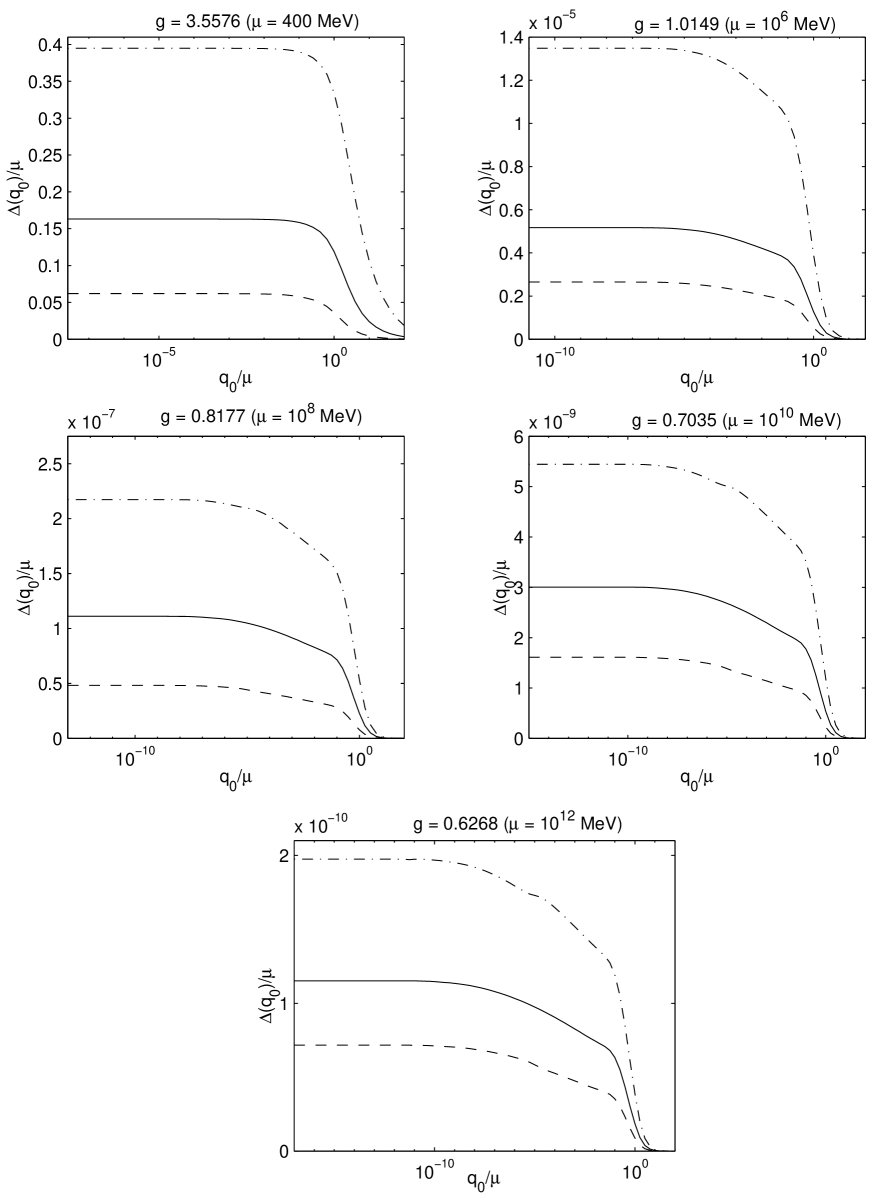
We have solved the gap equation (32) numerically for several different values of $g$ and several different values of $\xi$. It is convenient to change integration variables from $q_{0}$ to $\ln q_{0}$ and from $q$ to $\ln q$. We evaluate the $q$ integral over a range $q_{\rm min}<q<10^{4}\mu$ with $q_{\rm min}/\mu$ chosen differently for each $g$ in such a way that it is less than $10^{-5}\Delta(0)$ in all cases. The $q_{0}$ integral is made even in $q_{0}$ (by taking the average of the integrand at $q_{0}$ and $-q_{0}$) and then evaluated over a range $q_{0\rm min}<q_{0}<100\mu$, where we chose $q_{0\rm min}=q_{\rm min}$. We have checked that our results are insensitive to the choice of upper and lower cutoffs of the integration region. It was probably not necessary to choose $q_{\rm min}$ and $q_{0\rm min}$ quite as small as we did. It is, however, quite important to extend the upper limit of the $q_{0}$ and $q$ integrals to well above $\mu$ in order to avoid sensitivity to the ultraviolet cutoff. We use an iterative method, in which an initial guess for $\Delta(k_{0})$ is used on the right-hand side of (32), the integrals are done yielding a new $\Delta(k_{0})$, which is in turn used on the right-hand side. The solution converges well after about ten iterations. All results we show were iterated at least fifteen times.

FIG. 1.: The gap $\Delta(q_{0})$ for five different values of the coupling constant $g$. In each plot, the upper, middle, and lower curves are calculations done using three different gauges $\xi=-1,0,1$. In each panel, the range over which the $q_{0}$ integral was done is that shown.

Our results are shown in Fig. 1. Note that the output of our calculation is a plot of $\Delta(q_{0})/\mu$ as a function of $q_{0}/\mu$ for some choice of $g$ and $\xi$. The only way in which $\mu$ enters the calculation is to set the units of energy. The values of $\mu$ shown in Fig. 1 corresponding to each value of $g$ do not come from the calculation. They are obtained by assuming that the running coupling $g$ should be evaluated at the scale $\mu$ and using the one-loop beta function with $\Lambda_{\rm QCD}=200$ MeV. We include these values of $\mu$ to make comparison with the results of Refs. [24, 33] easier. If, as seems quite reasonable, $g$ should in fact be evaluated at a $g$-dependent scale which is lower than $\mu$, then the values of $g$ at which we have done our calculations correspond to larger values of $\mu$ than shown in Fig. 1 [31]. Evans, Hormuzdiar, Hsu, and Schwetz have obtained numerical solutions to simplified gap equations describing the gap in the CFL phase [33]. Their results agree reasonably well with the results of our calculation done in $\xi=0$ gauge but disagree qualitatively with ours in any other gauge. Simply setting $\xi=0$, as in Ref. [24, 33], is not a valid approximation at the values of $g$ at which we (and these authors) work.

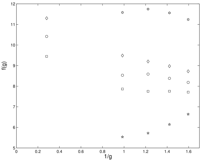
FIG. 2.: The function $f(g)$, defined in Eq. (70), for five different values of the coupling constant $g$. At each $g$, the points (from top to bottom) correspond to different gauges with $\xi=-4,-1,0,1,4$ respectively. Note that the horizontal axis is $1/g$ and $\mu$ increases to the right. At the largest value of g, we only show $\xi=-1,0,1$. In Fig. 1, we have not shown the $\Delta(q_{0})$ curves for $\xi=\pm 4$ because in these gauges $\Delta(q_{0})$ is very small or large on the scales of Fig. 1.

How should one interpret the results of a gauge dependent calculation, given that at any fixed $g$ one can obtain any result one likes if one is willing to explore gauge parameters $-\infty<\xi<\infty$? In the present circumstance, the idea is that we expect this calculation to give a gauge invariant result in the $g\rightarrow 0$ limit. More precisely, if we define

$$f(g)\equiv\ln\left[\frac{\Delta(0)}{\mu}\right]+\frac{3\pi^{2}}{\sqrt{2}g}+5\ln g$$ (70)

then we expect $f$ to go to a $\xi$-independent constant in the $g\rightarrow 0$ limit. In Fig. 2, we plot $f(g)$ in five different gauges. From this figure we learn:

• For any $\xi$, $f(g)$ is a reasonably slowly varying function of $g$. This confirms Son’s result (1) and justifies an analysis in terms of $f(g)$.

• It does appear that $\lim_{g\rightarrow 0}f(g)$ is a $\xi$-independent constant, perhaps not far from the estimate of Ref. [24], namely $\lim_{g\rightarrow 0}f(g)=8.88$, or that of Ref. [28], namely $\lim_{g\rightarrow 0}f(g)=7.84$.

• If we do a calculation in some fixed gauge, we expect that at small enough $g$ this calculation yields a good estimate of the true gauge invariant result. By doing calculations in several gauges, we can bound the regime of applicability of this estimate. We can only trust our calculation of $f(g)$ in the regime in which the $\xi$-dependence of $f$ decreases with decreasing $g$. Our calculation of $f(g)$ is completely meaningless unless $g$ is small enough that the curves for different values of $\xi$ are converging. Fig. 2 shows that the gauge dependence of our result for $f$ is about the same for all $g\gtrsim 0.8$. It is only for $g\lesssim 0.8$ that $f(g)$ calculated in different gauges begins to converge. At larger values of $g$ our calculation provides no guide whatsoever as to the value of $f$ that would be obtained in a complete, gauge invariant calculation including all the physics neglected in the present calculation. Even at $g=0.8$ the values of $\Delta(0)$ differ by a factor of about 400 for gaps with $\xi=-4$ and $\xi=4$. We could make the gauge dependence look even larger by choosing larger values of $|\xi|$. Our result does not guarantee that the calculation is under control for $g<0.8$, but it does guarantee that the result is uncontrolled and completely meaningless for $g>0.8$.

IV Conclusion

We have detailed our assumptions and approximations as we made them. Let us now ask which of them should be improved upon if we wish to include those contributions whose neglect we have diagnosed via the gauge dependence of our results. Note that $g=0.8$ corresponds to $\Delta/\mu\sim 10^{-7}$. Thus, those contributions to $f$ which we have neglected which are controlled when $\Delta\ll\mu$ are not responsible for the breakdown of our calculation around $g\sim 0.8$. We believe that the assumptions we made in writing the ansatz (5) and the assumptions we made in neglecting $\Delta_{1}^{S}$ and $\Delta^{A,S}_{2}$ all introduce errors which are small when $\Delta\ll\mu$. (For example, even though neglecting $\Delta_{2}$ is a source of gauge dependence, we do not expect that remedying this neglect would change $f(g)$ appreciably in any gauge at $g\sim 0.8$, where $\Delta/\mu$ is so small.) Hence, we believe that it is the assumptions made in writing the truncated gap equation (9) that are at fault. One obvious possible explanation is the absence of vertex corrections, although there are other missing skeleton diagrams which should also be investigated.

The gap $\Delta$ is of course a gauge invariant observable. A complete calculation would yield a gauge invariant expression for the function $f$, which could be expanded as a power series in $g$. We learn three things from our (incomplete and gauge dependent) calculation. First, our results obtained in different gauges appear to converge at small $g$ and support previous estimates of $\lim_{g\rightarrow 0}f(g)$, namely the $g^{0}$ term in the expansion of $f$. Second, because the results we obtain in different gauges only begin to converge for $g<g_{c}\sim 0.8$, we learn that contributions to our gauge dependent function $f$ which are of order $g^{1}$ and higher must have gauge dependent parts which are numerically large at $g\sim g_{c}$. Although we have simply evaluated $f(g)$ and not expanded it in $g$, we learn that such an expansion is uncontrolled for $g>g_{c}$. This suggests that if we knew the complete, gauge invariant function $f$, the $g^{1}$ and higher terms in that expansion would also become uncontrolled for $g>g_{c}$. It may be that the vertex corrections are the dominant contribution to the missing physics which is responsible for this breakdown: this hypothesis is supported by the arguments of Ref. [28] that these effects contribute to $f$ at order $g^{1}$. Regardless of whether the vertex corrections turn out to be the most important effect left out of the truncated gap equation (9), our calculation demonstrates that some contribution which is formally subleading is in fact large enough to render the calculation uncontrolled at $g\sim g_{c}$. The third thing we learn is that although present calculations do yield reasonable estimates of $\lim_{g\rightarrow 0}f(g)$, if one is interested in using these calculations to estimate the value of $\Delta$ to within a factor of two, this can only be done for $g\ll g_{c}\sim 0.8$.

In the CFL phase, all eight gluons get a mass. This means that in the CFL phase there are no gapless fermionic excitations, and no massless gluonic excitations, and therefore no non-Abelian physics in the infrared to obstruct weak-coupling calculations. The lesson we have learned is that even though everything is in principle under control, present weak-coupling calculations break down for $g>g_{c}\sim 0.8$, corresponding to $\mu<\mu_{c}$ with $\mu_{c}\sim 10^{8}$ MeV (or higher [31]). This break down occurs even though $\Delta\ll\mu$ at $g\sim g_{c}$. It should be noted that what breaks down is the weak-coupling calculation of the magnitude of the gap $\Delta$. Estimates based on models normalized to give reasonable zero density phenomenology can still be used as a guide, albeit a qualitative one. Furthermore, regardless of the fact that a controlled calculation of $\Delta$ has not yet been done at $\mu<10^{8}$ MeV, it is possible to construct a controlled effective field theory which describes the infrared physics of the CFL phase on length scales long compared to $1/\Delta$, since in such an effective theory $\Delta$ is simply a parameter determined by physics outside the effective theory. This infrared physics is dominated by the massless Abelian gauge bosons [10, 39], the Nambu-Goldstone boson arising from spontaneously broken $U(1)_{B}$ [10], and the pseudo-Nambu-Goldstone bosons arising from spontaneously broken chiral symmetry which have small masses due to the nonvanishing quark masses [10, 40, 41, 42, 43, 44, 45, 46, 47].

A The Meissner Effect

In this appendix, we set up the calculation of the Meissner effect. That is, we investigate the effect of the presence of a gap $\Delta$ on the functions $F$ and $G$ which describe the screening of the gluon propagator.

In order to establish some necessary notation, we must begin by filling in some details in the derivation of Eq. (11) from Eq. (9). We work in a color-flavor basis $(\{i,a\},\{j,b\})$. In this basis, we define the following two $9\times 9$ matrices:

$$Q^{ab}_{ij}=(\lambda^{A}_{I})^{ab}(\lambda^{A}_{I})_{ij}=\left(\begin{array}[]{ccccccccc}0&1&1&&&&&&\\ 1&0&1&&&&&&\\ 1&1&0&&&&&&\\ &&&0&-1&&&&\\ &&&-1&0&&&&\\ &&&&&0&-1&&\\ &&&&&-1&0&&\\ &&&&&&&0&-1\\ &&&&&&&-1&0\end{array}\right)$$ (A1)

$$R^{ab}_{ij}=(\lambda^{S}_{J})^{ab}(\lambda^{S}_{J})_{ij}=\left(\begin{array}[]{ccccccccc}2&1&1&&&&&&\\ 1&2&1&&&&&&\\ 1&1&2&&&&&&\\ &&&0&1&&&&\\ &&&1&0&&&&\\ &&&&&0&1&&\\ &&&&&1&0&&\\ &&&&&&&0&1\\ &&&&&&&1&0\end{array}\right)$$ (A2)

which represent the antisymmetric color and flavor ${\bar{\bf 3}}_{A}$ and the symmetric color and flavor ${\bf 6}_{S}$ channels respectively in this basis.

In the derivation of the gap equation, we were only interested in the off-diagonal lower left component of the Nambu-Gorkov fermion propagator $S$. However, the calculation of the Meissner effect involves all components of the fermion propagator. Obtaining the fermion propagator by inverting the inverse propagator (4) is straightforward but tedious. After a lot of algebra and using the ansatz (5) for the gap matrix, we find:

$$S(q)=\left(\begin{array}[]{cc}S_{11}(q)&S_{12}(q)\\ S_{21}(q)&S_{22}(q)\end{array}\right)$$ (A5)

where

$$S_{11}(q)=\left(\begin{array}[]{ccccccccc}A(q)&B(q)&B(q)&&&&&&\\ B(q)&A(q)&B(q)&&&&&&\\ B(q)&B(q)&A(q)&&&&&&\\ &&&C(q)&&&&&\\ &&&&C(q)&&&&\\ &&&&&C(q)&&&\\ &&&&&&C(q)&&\\ &&&&&&&C(q)&\\ &&&&&&&&C(q)\end{array}\right)$$ (A15)

$$S_{22}(q)=\left(\begin{array}[]{ccccccccc}E(q)&H(q)&H(q)&&&&&&\\ H(q)&E(q)&H(q)&&&&&&\\ H(q)&H(q)&E(q)&&&&&&\\ &&&D(q)&&&&&\\ &&&&D(q)&&&&\\ &&&&&D(q)&&&\\ &&&&&&D(q)&&\\ &&&&&&&D(q)&\\ &&&&&&&&D(q)\end{array}\right)$$ (A25)

$$S_{21}(q)=\overline{S_{12}}(q)=-\left(\begin{array}[]{ccccccccc}K(q)&L(q)&L(q)&&&&&&\\ L(q)&K(q)&L(q)&&&&&&\\ L(q)&L(q)&K(q)&&&&&&\\ &&&0&M(q)&&&&\\ &&&M(q)&0&&&&\\ &&&&&0&M(q)&&\\ &&&&&M(q)&0&&\\ &&&&&&&0&M(q)\\ &&&&&&&M(q)&0\end{array}\right)$$ (A35)

and where the above functions are defined as follows:

$$\begin{array}[]{ll}A(q)&=\gamma^{0}\left[P_{+}(q){q_{0}-\mu-|\vec{q}|\over q_{0}^{2}-(|\vec{q}|+\mu)^{2}-4({\Delta_{2}^{A}}(q_{0})+2{\Delta_{2}^{S}}(q_{0}))^{2}}{q_{0}^{2}-(|\vec{q}|+\mu)^{2}-3\left({\Delta_{2}^{A}}(q_{0})\right)^{2}-11\left({\Delta_{2}^{S}}(q_{0})\right)^{2}-10{\Delta_{2}^{A}}(q_{0}){\Delta_{2}^{S}}(q_{0})\over q_{0}^{2}-(|\vec{q}|+\mu)^{2}-({\Delta_{2}^{A}}(q_{0})-{\Delta_{2}^{S}}(q_{0}))^{2}}\right.\\ &+\left.P_{-}(q){q_{0}-\mu+|\vec{q}|\over q_{0}^{2}-(|\vec{q}|-\mu)^{2}-4({\Delta_{1}^{A}}(q_{0})+2{\Delta_{1}^{S}}(q_{0}))^{2}}{q_{0}^{2}-(|\vec{q}|-\mu)^{2}-3\left({\Delta_{1}^{A}}(q_{0})\right)^{2}-11\left({\Delta_{1}^{S}}(q_{0})\right)^{2}-10{\Delta_{1}^{A}}(q_{0}){\Delta_{1}^{S}}(q_{0})\over q_{0}^{2}-(|\vec{q}|-\mu)^{2}-({\Delta_{1}^{A}}(q_{0})-{\Delta_{1}^{S}}(q_{0}))^{2}}\right]\\ &\\ B(q)&=\gamma^{0}\left[P_{+}(q){q_{0}-\mu-|\vec{q}|\over q_{0}^{2}-(|\vec{q}|+\mu)^{2}-4({\Delta_{2}^{A}}(q_{0})+2{\Delta_{2}^{S}}(q_{0}))^{2}}{\left({\Delta_{2}^{A}}(q_{0})+5{\Delta_{2}^{S}}(q_{0})\right)\left({\Delta_{2}^{A}}(q_{0})+{\Delta_{2}^{S}}(q_{0})\right)\over q_{0}^{2}-(|\vec{q}|+\mu)^{2}-({\Delta_{2}^{A}}(q_{0})-{\Delta_{2}^{S}}(q_{0}))^{2}}\right.\\ &+\left.P_{-}(q){q_{0}-\mu+|\vec{q}|\over q_{0}^{2}-(|\vec{q}|-\mu)^{2}-4({\Delta_{1}^{A}}(q_{0})+2{\Delta_{1}^{S}}(q_{0}))^{2}}{\left({\Delta_{1}^{A}}(q_{0})+5{\Delta_{1}^{S}}(q_{0})\right)\left({\Delta_{1}^{A}}(q_{0})+{\Delta_{1}^{S}}(q_{0})\right)\over q_{0}^{2}-(|\vec{q}|-\mu)^{2}-({\Delta_{1}^{A}}(q_{0})-{\Delta_{1}^{S}}(q_{0}))^{2}}\right]\end{array}$$ (A36)

$$\begin{array}[]{ll}C(q)&=\gamma^{0}\left[P_{+}(q){q_{0}-\mu-|\vec{q}|\over q_{0}^{2}-(|\vec{q}|+\mu)^{2}-({\Delta_{2}^{A}}(q_{0})-{\Delta_{2}^{S}}(q_{0}))^{2}}+P_{-}(q){q_{0}-\mu+|\vec{q}|\over q_{0}^{2}-(|\vec{q}|-\mu)^{2}-({\Delta_{1}^{A}}(q_{0})-{\Delta_{1}^{S}}(q_{0}))^{2}}\right]\\ &\\ D(q)&=C\gamma^{0}\left[P_{-}(q){q_{0}+\mu+|\vec{q}|\over q_{0}^{2}-(|\vec{q}|+\mu)^{2}-({\Delta_{2}^{A}}(q_{0})-{\Delta_{2}^{S}}(q_{0}))^{2}}+P_{+}(q){q_{0}+\mu-|\vec{q}|\over q_{0}^{2}-(|\vec{q}|-\mu)^{2}-({\Delta_{1}^{A}}(q_{0})-{\Delta_{1}^{S}}(q_{0}))^{2}}\right]C\\ &\\ E(q)&=C\gamma^{0}\left[P_{-}(q){q_{0}+\mu+|\vec{q}|\over q_{0}^{2}-(|\vec{q}|+\mu)^{2}-4({\Delta_{2}^{A}}(q_{0})+2{\Delta_{2}^{S}}(q_{0}))^{2}}{q_{0}^{2}-(|\vec{q}|+\mu)^{2}-3\left({\Delta_{2}^{A}}(q_{0})\right)^{2}-11\left({\Delta_{2}^{S}}(q_{0})\right)^{2}-10{\Delta_{2}^{A}}(q_{0}){\Delta_{2}^{S}}(q_{0})\over q_{0}^{2}-(|\vec{q}|+\mu)^{2}-({\Delta_{2}^{A}}(q_{0})-{\Delta_{2}^{S}}(q_{0}))^{2}}\right.\\ &+\left.P_{+}(q){q_{0}+\mu-|\vec{q}|\over q_{0}^{2}-(|\vec{q}|-\mu)^{2}-4({\Delta_{1}^{A}}(q_{0})+2{\Delta_{1}^{S}}(q_{0}))^{2}}{q_{0}^{2}-(|\vec{q}|-\mu)^{2}-3\left({\Delta_{1}^{A}}(q_{0})\right)^{2}-11\left({\Delta_{1}^{S}}(q_{0})\right)^{2}-10{\Delta_{1}^{A}}(q_{0}){\Delta_{1}^{S}}(q_{0})\over q_{0}^{2}-(|\vec{q}|-\mu)^{2}-({\Delta_{1}^{A}}(q_{0})-{\Delta_{1}^{S}}(q_{0}))^{2}}\right]C\\ &\\ H(q)&=C\gamma^{0}\left[P_{-}(q){q_{0}+\mu+|\vec{q}|\over q_{0}^{2}-(|\vec{q}|+\mu)^{2}-4({\Delta_{2}^{A}}(q_{0})+2{\Delta_{2}^{S}}(q_{0}))^{2}}{\left({\Delta_{2}^{A}}(q_{0})+5{\Delta_{2}^{S}}(q_{0})\right)\left({\Delta_{2}^{A}}(q_{0})+{\Delta_{2}^{S}}(q_{0})\right)\over q_{0}^{2}-(|\vec{q}|+\mu)^{2}-({\Delta_{2}^{A}}(q_{0})-{\Delta_{2}^{S}}(q_{0}))^{2}}\right.\\ &+\left.P_{+}(q){q_{0}+\mu-|\vec{q}|\over q_{0}^{2}-(|\vec{q}|-\mu)^{2}-4({\Delta_{1}^{A}}(q_{0})+2{\Delta_{1}^{S}}(q_{0}))^{2}}{\left({\Delta_{1}^{A}}(q_{0})+5{\Delta_{1}^{S}}(q_{0})\right)\left({\Delta_{1}^{A}}(q_{0})+{\Delta_{1}^{S}}(q_{0})\right)\over q_{0}^{2}-(|\vec{q}|-\mu)^{2}-({\Delta_{1}^{A}}(q_{0})-{\Delta_{1}^{S}}(q_{0}))^{2}}\right]C\\ &\\ K(q)&=2C\gamma^{5}\left[P_{+}(q)\left({{\Delta_{2}^{S}}(q_{0})\over q_{0}^{2}-(|\vec{q}|+\mu)^{2}-4({\Delta_{2}^{A}}(q_{0})+2{\Delta_{2}^{S}}(q_{0}))^{2}}\right.\right.\\ &\qquad\qquad\qquad\left.+{{\Delta_{2}^{A}}(q_{0})-{\Delta_{2}^{S}}(q_{0})\over q_{0}^{2}-(|\vec{q}|+\mu)^{2}-4({\Delta_{2}^{A}}(q_{0})+2{\Delta_{2}^{S}}(q_{0}))^{2}}{\left({\Delta_{2}^{A}}(q_{0})+5{\Delta_{2}^{S}}(q_{0})\right)\left({\Delta_{2}^{A}}(q_{0})+{\Delta_{2}^{S}}(q_{0})\right)\over q_{0}^{2}-(|\vec{q}|+\mu)^{2}-({\Delta_{2}^{A}}(q_{0})-{\Delta_{2}^{S}}(q_{0}))^{2}}\right)\\ &+\left.P_{-}(q)\left({{\Delta_{1}^{S}}(q_{0})\over q_{0}^{2}-(|\vec{q}|-\mu)^{2}-4({\Delta_{1}^{A}}(q_{0})-2{\Delta_{1}^{S}}(q_{0}))^{2}}\right.\right.\\ &\qquad\qquad\qquad\left.\left.+{{\Delta_{1}^{A}}(q_{0})-{\Delta_{1}^{S}}(q_{0})\over q_{0}^{2}-(|\vec{q}|-\mu)^{2}-4({\Delta_{1}^{A}}(q_{0})+2{\Delta_{1}^{S}}(q_{0}))^{2}}{\left({\Delta_{1}^{A}}(q_{0})+5{\Delta_{1}^{S}}(q_{0})\right)\left({\Delta_{1}^{A}}(q_{0})+{\Delta_{1}^{S}}(q_{0})\right)\over q_{0}^{2}-(|\vec{q}|-\mu)^{2}-({\Delta_{1}^{A}}(q_{0})-{\Delta_{1}^{S}}(q_{0}))^{2}}\right)\right]\\ &\\ L(q)&=C\gamma^{5}\left[P_{+}(q)\left({{\Delta_{2}^{S}}(q_{0})+{\Delta_{2}^{A}}(q_{0})\over q_{0}^{2}-(|\vec{q}|+\mu)^{2}-4({\Delta_{2}^{A}}(q_{0})+2{\Delta_{2}^{S}}(q_{0}))^{2}}\right.\right.\\ &\qquad\qquad\qquad\left.\left.+{-{\Delta_{2}^{A}}(q_{0})+{\Delta_{2}^{S}}(q_{0})\over q_{0}^{2}-(|\vec{q}|+\mu)^{2}-4({\Delta_{2}^{A}}(q_{0})+2{\Delta_{2}^{S}}(q_{0}))^{2}}{\left({\Delta_{2}^{A}}(q_{0})+5{\Delta_{2}^{S}}(q_{0})\right)\left({\Delta_{2}^{A}}(q_{0})+{\Delta_{2}^{S}}(q_{0})\right)\over q_{0}^{2}-(|\vec{q}|+\mu)^{2}-({\Delta_{2}^{A}}(q_{0})-{\Delta_{2}^{S}}(q_{0}))^{2}}\right)\right.\\ &+\left.P_{-}(q)\left({{\Delta_{1}^{S}}(q_{0})+{\Delta_{1}^{A}}(q_{0})\over q_{0}^{2}-(|\vec{q}|-\mu)^{2}-4({\Delta_{1}^{A}}(q_{0})+2{\Delta_{1}^{S}}(q_{0}))^{2}}\right.\right.\\ &\qquad\qquad\qquad\left.\left.+{-{\Delta_{1}^{A}}(q_{0})+{\Delta_{1}^{S}}(q_{0})\over q_{0}^{2}-(|\vec{q}|-\mu)^{2}-4({\Delta_{1}^{A}}(q_{0})+2{\Delta_{1}^{S}}(q_{0}))^{2}}{\left({\Delta_{1}^{A}}(q_{0})+5{\Delta_{1}^{S}}(q_{0})\right)\left({\Delta_{1}^{A}}(q_{0})+{\Delta_{1}^{S}}(q_{0})\right)\over q_{0}^{2}-(|\vec{q}|-\mu)^{2}-({\Delta_{1}^{A}}(q_{0})-{\Delta_{1}^{S}}(q_{0}))^{2}}\right)\right]\\ &\\ M(q)&=C\gamma^{5}\left[P_{+}(q){-{\Delta_{2}^{A}}(q_{0})+{\Delta_{2}^{S}}(q_{0})\over q_{0}^{2}-(|\vec{q}|+\mu)^{2}-({\Delta_{2}^{A}}(q_{0})-{\Delta_{2}^{S}}(q_{0}))^{2}}+P_{-}(q){-{\Delta_{1}^{A}}(q_{0})+{\Delta_{1}^{S}}(q_{0})\over q_{0}^{2}-(|\vec{q}|-\mu)^{2}-({\Delta_{1}^{A}}(q_{0})-{\Delta_{1}^{S}}(q_{0}))^{2}}\right].\end{array}$$ (A36)

Note that $S_{21}(q)=\overline{S_{12}}(q)$ is a general property of the Fermion propagator $S$ and can be proved for an arbitrary number of colors and flavors using only the definition of the inverse Fermion propagator, Eq. (4), and properties of the Dirac gamma matrices. Whereas only $K$, $L$ and $M$ were used in the derivation of the gap equation, all these functions are required in evaluating the Meissner effect.

FIG. 3.: One-loop contribution to the Meissner effect.

The Meissner effect is the change in the screening of the gluon propagator induced by the presence of a gap. To one loop order, we need to evaluate the gluon propagator of Fig. 3 using the full fermion propagator including the gap. The result can still be written in the form (21) but now

$$F(q)=F_{0}(q)+\delta F(q)\ \ {\rm and}\ \ G(q)=G_{0}(q)+\delta G(q)$$ (A37)

where $F_{0}$ and $G_{0}$ are the $\Delta=0$ functions written as $F$ and $G$ in (23). Recall that $G_{0}$, which describes Landau damping, vanishes for $q_{0}\rightarrow 0$. Because $\delta G$ is nonzero in the $q_{0}\rightarrow 0$ limit, the Meissner effect can be described as giving a mass to the gluons. Previous analyses of the Meissner effect have either been done for two-flavor QCD [48, 49] or have used simplified estimates [27, 32, 33]. Our goal is to formulate the correct calculation of $\delta F(q)$ and $\delta G(q)$ in the CFL phase. Recent work along the same lines can be found in Ref. [50].

From the diagram of Fig. 3, we obtain the gluon polarization

$$\begin{array}[]{lll}\Pi^{\mu\nu}_{ab}&=-ig^{2}\int{d^{4}k\over(2\pi)^{4}}{\rm Tr}&\left[\Gamma^{\mu}_{a}S(k+q)\Gamma^{\nu}_{b}S(k)\right]\\ &=-ig^{2}\int{d^{4}k\over(2\pi)^{4}}{\rm Tr}&\left[\gamma^{\mu}{\lambda_{a}\over 2}S_{11}(k+q)\gamma^{\nu}{\lambda_{b}\over 2}S_{11}(k)+\left(\gamma^{\mu}{\lambda_{a}\over 2}\right)^{T}S_{22}(k+q)\left(\gamma^{\nu}{\lambda_{b}\over 2}\right)^{T}S_{22}(k)\right.\\ &&\left.-\gamma^{\mu}{\lambda_{a}\over 2}S_{12}(k+q)\left(\gamma^{\nu}{\lambda_{b}\over 2}\right)^{T}S_{21}(k)-\left(\gamma^{\mu}{\lambda_{a}\over 2}\right)^{T}S_{21}(k+q)\gamma^{\nu}{\lambda_{b}\over 2}S_{12}(k)\right],\end{array}$$ (A38)

where the trace is taken over color, flavor, and Dirac indices and all four elements of the fermion propagator, $S(q)$, have been defined previously in Eqs. (A15) – (A36). This polarization amplitude contains all the one loop contributions to the gluon propagator including the gap independent contributions, $F_{0}(q)$ and $G_{0}(q)$. $\Pi^{\mu\nu}_{ab}$ can be written in terms of $F$ and $G$ in a simple fashion:

$$\Pi^{\mu\nu}_{ab}=\delta_{ab}\left[\left(G_{0}(q)+\delta G(q)\right)P^{\mu\nu T}+\left(F_{0}(q)+\delta F(q)\right)P^{\mu\nu L}\right].$$ (A39)

Hence, we only need to compute two components of $\Pi^{\mu\nu}_{ab}$ in order to obtain the functions $\delta F(q)$ and $\delta G(q)$, for example, $\Pi_{33}^{00}$ and $\Pi_{33}^{11}$. Because we already know $F_{0}(q)$ and $G_{0}(q)$, our goal is to extract $\delta F(q)$ and $\delta G(q)$. We are therefore only interested in the difference $\Pi^{\mu\nu}_{ab}(\Delta\neq 0)-\Pi^{\mu\nu}_{ab}(\Delta=0)$. Finally, because $\delta F(q)$ and $\delta G(q)$ depend only on $q_{0}$ and $|\vec{q}|$, we can choose $\vec{q}$ to lie along the $z$-axis for simplicity. Keeping all this in mind, we find that (in Euclidean space)

$$\delta F(q)={q_{0}^{2}+|\vec{q}|^{2}\over|\vec{q}|^{2}}\left(\Pi^{00}_{33}(\Delta\neq 0)-\Pi^{00}_{33}(\Delta=0)\right)$$ (A40)

$$\delta G(q)=\Pi^{11}_{33}(\Delta\neq 0)-\Pi^{11}_{33}(\Delta=0).$$ (A41)

Note that (unlike the integrals which arise on the right hand side of the gap equation) the integrals which must be done in evaluating $\Pi(q)$ are ultraviolet divergent, and therefore sensitive to how they are cutoff at large $k_{0}$ and $k$. This ultraviolet divergence has nothing to do with $\Delta$, and is canceled in our calculation of $\delta F$ and $\delta G$ by subtracting the $\Delta=0$ result for $\Pi(q)$. We have checked that our results for $\delta F$ and $\delta G$ are insensitive to the ultraviolet cutoffs in the integrals.

Looking back at the definition of $\Pi^{\mu\nu}_{ab}$, we can see that it depends on $\Delta_{1}^{A,S}(k_{0})$ and $\Delta_{2}^{A,S}(k_{0})$. We make the same assumptions here as in our solution of the gap equation, namely that the antiparticle and sextet contributions can be neglected if $\Delta\ll\mu$ and if one is interested in physics dominated by particles and holes near the Fermi surface. Before we proceed, let us define the following notation for the functions $A(q)$ through $M(q)$ defined in Eq. (A36): identify the scalar functions multiplying the $P_{\pm}$ projectors with the appropriate $\pm$ signs, e.g. $A_{+}(q)$. With this notation, the dominant contributions to the two polarization amplitudes we are interested in are:

$$\begin{array}[]{ll}\Pi^{00}_{33}=-{i\over 2}g^{2}\!\int\!{d^{4}k\over(2\pi)^{4}}&\!\left(1+\widehat{(k+q)}\cdot\hat{k}\right)\left[A_{-}(k+q)A_{-}(k)-B_{-}(k+q)B_{-}(k)\right.\\ &+2C_{-}(k+q)C_{-}(k)+E_{+}(k+q)E_{+}(k)-H_{+}(k+q)H_{+}(k)\\ &+2D_{+}(k+q)D_{+}(k)-2K_{-}(k+q)K_{-}(k)\\ &\left.+2L_{-}(k+q)L_{-}(k)+2M_{-}(k+q)M_{-}(k)\right]\\ \Pi^{11}_{33}=-{i\over 2}g^{2}\!\int\!{d^{4}k\over(2\pi)^{4}}&\!\left(1+2\widehat{(k+q)}^{1}\hat{k}^{1}-\widehat{(k+q)}\cdot\hat{k}\right)\left[A_{-}(k+q)A_{-}(k)\right.\\ &-B_{-}(k+q)B_{-}(k)+2C_{-}(k+q)C_{-}(k)+E_{+}(k+q)E_{+}(k)\\ &-H_{+}(k+q)H_{+}(k)+2D_{+}(k+q)D_{+}(k)+2K_{-}(k+q)K_{-}(k)\\ &\left.-2L_{-}(k+q)L_{-}(k)-2M_{-}(k+q)M_{-}(k)\right].\end{array}$$ (A42)

In any one gauge, i.e. for a particular choice of $\xi$, our task is now clear. We first calculate $\Delta(k_{0})$ with $\delta F(q)=\delta G(q)=0$, as described in the body of the paper. We must then use (A42) to evaluate $\delta F(q)$ and $\delta G(q)$ given by Eq. (A40). As in the calculation of $\Delta$, we can do all angular integrals analytically and evaluate the double integral over $k_{0}$ and $|{\vec{k}}|$ numerically. We must then re-evaluate $\Delta(k_{0})$ with the new gluon propagator, modified by the addition of $\delta F(q)$ and $\delta G(q)$. We must then iterate this procedure, calculating $\delta F(q)$ and $\delta G(q)$ and then recalculating $\Delta(k_{0})$ repeatedly, until all results have converged. We have not carried this program to completion. However, preliminary numerical investigation suggests that, in agreement with arguments and estimates made by others [23, 24, 27, 29, 32, 33], the change in $\Delta$ arising from the inclusion of $\delta F$ and $\delta G$ is small. In particular, it appears to be much smaller than the change in $\Delta$ which arises if one changes gauge from $\xi=-1$ to $\xi=0$ to $\xi=1$. Perhaps at some extremely small $g$, the influence of the Meissner effect on the gap could be larger than the influence of the neglected physics whose absence we diagnose via the gauge dependence of our results. At any $g$ at which we have been able to obtain numerical results, however, the Meissner effect is insignificant relative to that which is missing.