R-Parity Violation and the Decay $b\rightarrow s\gamma$

Abstract

We investigate the influence of the R-parity violating couplings $\lambda$, $\lambda^{\prime}$ and $\lambda^{\prime\prime}$ on the branching ratio of $b\rightarrow s\gamma$ in leading logarithmic approximation. The operator basis is enlarged and the corresponding $\gamma$-matrix calculated. The matching conditions receive new contributions from the R-parity violating sector. The comparison with the experiment is rather difficult due to the model dependence of the result.

I Introduction

The decay $b\rightarrow s\gamma$, forbidden at tree-level in the Standard Model (SM), is an excellent candidate for exploring the influence of new physics beyond the SM. However, the experimentally measured branching ratio $\mbox{Br}(B\rightarrow X_{s}\gamma)=(3.15\pm 0.93)\cdot 10^{-4}$ [1] is in perfect agreement with the SM prediction computed at the next-to-leading order:$\mbox{Br}(b\rightarrow s\gamma)_{SM}=(3.28\pm 0.30)\cdot 10^{-4}$ [2]. This leads to the conclusion that the influence of new physics on this decay is either very limited or the new contributions cancel among each other to a large extent. The most serious and attractive extention of the Standard Model is Supersymmetry (SUSY). It has a variety of very appealing features. For instance it provides a natural solution to the hierarchy problem. SUSY doubles the particle spectrum of the SM providing every fermion with a bosonic partner and vice versa. If SUSY were an exact symmetry of nature the new particles would be of the same mass as their partners. This is definitely excluded from experiment. Therefore SUSY must be broken. To retain the solution of the hierarchy problem one allows only a breaking which does not introduce quadratic divergences in loop diagrams. Although this reduces the set of possible breaking terms substantially to the so-called soft-breaking terms the number of free parameters of softly broken SUSY still exceeds one hundred. This theory, i.e., SUSY with soft breaking terms and no others, emerges naturally as low energy limit of local supersymmetry, Supergravity (SUGRA) by breaking it at some high scale $\sim 10^{11}$ GeV and taking the so-called flat limit [3]. The connection to supergravity eliminates much of the freedom in choosing the parameters for the soft breaking terms, enhancing the predictive power of the model.
Viewing naturalness as a first principle in model building one runs immediately into a problem: The Yukawa interactions are fixed by the so-called Superpotential $W$, which is the most general third degree polynomial that can be built of gauge invariant combinations of the (left-handed) superfields of the theory. In the case of the minimal extension of the standard model with gauge group $SU(3)\times SU(2)\times U(1)$ it shows the form

$$W = \lambda^{u}_{ij}Q_{i}H_{2}U_{j}^{c}+\lambda^{d}_{ij}H_{1}Q_{i}D_{j}^{c}+\lambda^{e}_{ij}H_{1}L_{i}E_{j}^{c}+\mu H_{1}H_{2}$$ (2)

$$+\mu_{2i}L_{i}H_{2}+\frac{1}{2}\lambda_{ijk}L_{i}L_{j}E_{k}^{c}+\lambda^{\prime}_{ijk}L_{i}Q_{j}D_{k}^{c}+\frac{1}{2}\lambda^{\prime\prime}_{ijk}U_{i}^{c}D_{j}^{c}D_{k}^{c},$$

where $Q,\,U^{c},\,D^{c},\,L,\,E^{c},\,H_{1}$ and $H_{2}$ label the left-handed superfields that describe left- and right-handed (s)quarks and (s)leptons and the Higgs-bosons (-fermions) respectively. The terms on the second line of (2) lead to unwanted baryon- and lepton-number violating vertices. The product $\lambda^{\prime}_{ijk}\cdot\lambda^{\prime\prime}_{ijk}$, for instance, is restricted to be smaller than $10^{-10}$ [4]. It is not obvious why the coefficients of these terms should not be of order unity if the corresponding interaction is not protected by any symmetry. Hence one way to avoid these unwanted couplings is the invention of a new discrete symmetry, called R-Parity [5]. The multiplicative quantum number $R$ is then defined as

$$R=(-1)^{3B+L+2s},$$ (3)

where $s$ is the spin of the particle. The particles of the standard model are then R-parity even fields while their supersymmetric partners are R-parity odd fields. The superfields adopt the value of R from their scalar components. The terms on the second line of (2) are then forbidden by this symmetry. One ends up with the Minimal Supersymmetric Standard Model (MSSM) [6, 7, 8]. One could even go one step further and promote this new symmetry to a $U(1)$ gauge symmetry (R-symmetry). The R-charges must then be chosen such that the “nice” terms remain in the Lagrangian and the unwanted terms will not be allowed anymore. Further requirement is the vanishing of possible additional anomalies [9, 10]. This scenario is preferred from a string theoretical view because in string theory one has many additional $U(1)$’s “floating around”, what makes the introduction of this symmetry more natural.
It is interesting to explore what the constraints on the R-parity violating couplings, especially $\lambda_{ijk}$, $\lambda^{\prime}_{ijk}$, and $\lambda^{\prime\prime}_{ijk}$, are from the experimental point of view. Bounds on these couplings have been found by many authors [11, 12, 13, 14]. Sometimes the bounds on products of couplings are more restrictive than the products of the individual bounds. Depending on the reactions that the couplings are involved in the constraints from experiment are very strong or rather poor.
In this paper we want to explore the (theoretical) influence of $\lambda$, $\lambda^{\prime}$, and $\lambda^{\prime\prime}$ on the decay $b\rightarrow s\gamma$. This has been done before by other authors [15]. However, here we will include the full operator basis at leading-log of the effective low-energy theory.
The comparison with the experiment must result in bounds that are model dependent. The relevant couplings are proportional to the inverse mass-squared of particles (Higgs, SUSY-partners) that have not yet been detected. However, it is clear from next-to-leading-log calculations that the prediction of the MSSM with a realistic mass spectrum lies within the current experimental bounds.
Because of the strong model dependence we do not perform our calculations at highest precision. Nevertheless we try to include all the possibly relevant contributions at leading-log. We do not claim our results to be very accurate. It is the aim of this paper to explore if $b\rightarrow s\gamma$ has the potential power to reduce the bounds of (products of) some of the R-parity breaking couplings substantially, i.e., by some order of magnitude.
This article is divided as follows: Section 2 introduces the model we are working with. We try to describe as precise as possible what our assumptions are. The following section deals with the effective Hamiltonian approach. The enhanced operator basis is presented and the $\gamma$-matrix as well as the matching conditions at $M_{W}$ calculated. The comparison with the experiment is performed in section 4. Section 5 contains our conclusions. In the appendix we present some technical details of our computations, namely the mixing matrices,the relevant part of the interaction Lagrangian and the RGE’s that are needed.

II Framework

In supersymmetry the matter fields are described by left-handed chiral superfields $\Sigma^{i}$. They contain a scalar boson $z^{i}$ and a two-component fermion $\psi^{i}$. Real vector superfields $V^{a}$ are needed to form the gauge bosons $A^{a}_{\mu}$ and the gauginos $\lambda^{a}$. The minimal supersymmetric standard model is the model with the smallest particle content that is able to mimic the features of the standard model, i.e., including all the observed particles, gauge group $SU(3)_{\mathrm{colour}}\times SU(2)_{\mathrm{weak}}\times U(1)_{Y}$, spontaneous symmetry breaking and the Higgs mechanism. Its superfields together with their components are collected in table I. A few comments are in order:

• Because the theory only deals with left-handed chiral superfields the $SU(2)$-singlet matter fields must be defined via their charged conjugated (anti-) fields.

• No conjugated superfields are allowed in the superpotential $W$. Therefore we need to introduce a second Higgs field to give the up and the down quarks a mass when the neutral components gain a vacuum expectation value (vev).

• The $L$’s and $R$’s in the names of squarks and sleptons only identify the fermionic partners. These fields are just normal complex scalar bosons.

It must be mentioned that the fields in table I are not the physical fields.

• In the Higgs sector three degrees of freedom are eaten by the gauge bosons in analogy to the SM. We end up with one charged and three neutral Higgs bosons.

• Higgsinos and gauginos of $SU(2)\times U(1)$ mix to form charginos and neutralinos.

• Photon, $W$- and $Z$-boson form when the electroweak symmetry breaks down.

• The three generations of quarks and leptons mix via the Cabibbo-Kobayashi-Maskawa-matrix $K$ to give the mass eigenstates in complete analogy to the standard model.

• The family mixing also takes place in the squark and slepton sector. However, there is an additional mixing between the partners of left- and right-handed fermions due to the soft-breaking terms.

Appendix A gives a more detailed description of the different mixings including a complete listing of all relevant mixing matrices.

The component expression of the Lagrangian we base our model on can be written as

$${\mathcal{L}}={\mathcal{L}}_{\mathrm{kin}}+{\mathcal{L}}_{\mathrm{int}}+{\mathcal{L}}_{W}-V_{\mathrm{soft}},$$ (4)

where

• ${\mathcal{L}}_{\mathrm{kin}}$ and ${\mathcal{L}}_{\mathrm{int}}$ stand for the kinetic energies, the interactions between chiral and gauge fields and part of the scalar potential.

• ${\mathcal{L}}_{W}$ contains the rest of the scalar potential and the Yukawa interactions:

  $${\mathcal{L}}_{W}=-\sum_{i}\left|\frac{\partial W}{\partial z_{i}}\right|^{2}-\frac{1}{2}\sum_{ij}\left[\psi_{i}\frac{\partial^{2}W}{\partial z_{i}\partial z_{j}}\psi_{j}+\mbox{h.c.}\right],$$ (5)

  where $W$ should be viewed as a function of the scalar fields.

• $W$ is the superpotential which contains all possible gauge invariant combinations of the left-handed superfields (but not their conjugated right-handed partners). In our case, this results in equation (2). It should be noted that every term is a gauge invariant combination of the corresponding superfields, for instance, $Q_{i}H_{2}U_{j}^{c}$ is abbreviated for $\epsilon_{\alpha\beta}\,Q_{i}^{\alpha A}\,H_{2}^{\beta}\,U_{j}^{cA}$, where $\alpha$ and $\beta$ are $SU(2)$-indices, $A$ is an $SU(3)$-index and $\epsilon_{\alpha\beta}$ is the completely antisymmetric tensor with $\epsilon_{12}=1$ . The second line of (2) represents the R-parity breaking sector. As a consequence of the antisymmetry in the fields $\lambda$ is antisymmetric in its first two indices and $\lambda^{\prime\prime}$ is antisymmetric in its last two indices. Therefore the trilinear R-parity breaking couplings of $W$ contain $9+27+9=45$ new parameters.

• $V_{\mathrm{soft}}$ includes the soft-breaking trilinear terms of the scalar potential and mass terms for the scalar fields and the gauginos. It has the form

  $$V_{\mathrm{soft}} = [h^{u}_{ij}\tilde{q}_{i}\tilde{h}_{2}\tilde{u}_{j}^{\dagger}+h^{d}_{ij}\tilde{h}_{1}\tilde{q}_{i}\tilde{d}_{j}^{\dagger}+h^{e}_{ij}\tilde{h}_{1}\tilde{\ell}_{i}\tilde{e}_{j}^{\dagger}$$ (9)

  $$+\frac{1}{2}C_{ijk}\tilde{\ell}_{i}\tilde{\ell}_{j}\tilde{e}^{\dagger}_{k}+C^{\prime}_{ijk}\tilde{\ell}_{i}\tilde{q}_{j}\tilde{d}^{\dagger}_{k}+\frac{1}{2}C^{\prime\prime}_{ijk}\tilde{u}^{\dagger}_{i}\tilde{d}^{\dagger}_{j}\tilde{d}^{\dagger}_{k}$$

  $$+\tilde{\mu}\tilde{h}_{1}\tilde{h}_{2}+\tilde{\mu}_{2i}\tilde{\ell}_{i}\tilde{h}_{2}]+\mbox{h.c.}+m_{ab}^{2}z^{a}z^{b\dagger}$$

  $$+\frac{1}{2}M_{a}[\lambda_{a}\lambda_{a}+\mbox{h.c.}].$$

The MSSM in its full generality with an additional R-parity breaking sector involves over 150 free parameters. These are by far too many for the model to be predictive. In the following we will reduce the parameter space substantially by making some assumptions that are, hopefully, well motivated.
As a first step it is important to mention that we see our softly broken global SUSY at a low energy scale $\sim M_{Z}$ emerging from a spontaneously broken local supersymmetry at a high scale $M_{X}\sim 10^{16}$ GeV taking the flat limit $M_{\mathrm{Planck}}\rightarrow\infty$, $m_{0}:=m_{\mathrm{gravitino}}=$constant. This fixes most of the parameters of $V_{\mathrm{soft}}$ at $M_{X}$:

• All the coefficients of the trilinear terms in $V_{\mathrm{soft}}$ are related to the corresponding terms of $W$ by a multiplication with a universal factor $Am_{0}$:

  $$\begin{array}[]{lcl}h^{u}_{ij}=Am_{0}\lambda^{u}_{ij}\hskip 28.45274pt&C_{ijk}=Am_{0}\lambda_{ijk}\\ \\ h^{d}_{ij}=Am_{0}\lambda^{d}_{ij}\hskip 28.45274pt&C^{\prime}_{ijk}=Am_{0}\lambda^{\prime}_{ijk}\\ \\ h^{e}_{ij}=Am_{0}\lambda^{e}_{ij}\hskip 28.45274pt&C^{\prime\prime}_{ijk}=Am_{0}\lambda^{\prime\prime}_{ijk}\end{array}$$ (10)

• An analogous statement holds for the bilinear terms:

  $$\tilde{\mu}=Bm_{0}\mu\hskip 28.45274pt \tilde{\mu}_{2i}=Bm_{0}\mu_{2i},$$ (11)

  where usually

  $$B=A-1.$$ (12)

• The mass term of the scalars are diagonal and universally equal to the gravitino mass $m_{0}$:

  $$m_{ab}^{2}=m_{0}^{2}\delta_{ab}$$ (13)

We assume unification of the gauge group at $M_{X}$. As a consequence all the gaugino masses are equal at that scale:

$$M_{i}(M_{X})=M\hskip 28.45274pt\forall i$$ (14)

Not all entries of the Yukawa-matrices $\lambda^{u}_{ij}$, $\lambda^{d}_{ij}$, and $\lambda^{e}_{ij}$ are observable in the SM. One usually chooses two of them (in most cases $\lambda^{d}$ and $\lambda^{e}$) to be diagonal. Although this is in principle not possible in our model we will adopt this choice here for convenience. All the entries at $M_{W}$ are then fixed by the quark/lepton masses, the vevs $v_{1}$ and $v_{2}$ of the neutral Higgs bosons $H_{1}$ and $H_{2}$ respectively and the Cabibbo-Kobayashi-Maskawa-matrix $K$.

$\mu H_{1}H_{2}$ is the so-called $\mu$-term. The mass parameter $\mu$ must be of order of the weak scale whereas the natural scale would be the Planck mass $M_{P}\sim 10^{19}$ GeV. The question why this parameter is so small is referred to as the $\mu$-problem.

$\mu_{2i}L_{i}H_{2}$ and $\tilde{\mu}_{2i}\tilde{\ell}_{i}\tilde{h}_{2}$ mix Higgs and leptonic sector. We choose to set $\mu_{2i}(M_{X})=\tilde{\mu}_{2i}(M_{X})=0$. At $M_{Z}$, $\mu_{2i}L_{i}H_{2}$ can be rotated away with the help of a field redefinition of the Higgs field whereas $\tilde{\mu}_{2i}$ is, at least in the case of a physically realistic spectrum, small enough to be neglected.
One ends up with the following free parameters:

$$A,\;m_{0},\;M,\;\mu$$ (15)

Usually, one replaces one of these parameters by $\tan\beta=v_{2}/v_{1}$. A second parameter will be fixed by the requirement of a correct electroweak symmetry breaking. This means, the minimum of the scalar Higgs potential must occur at values $(v_{1},v_{2})$ which reproduce the correct mass of the $Z$-boson:

$$M_{Z}^{2}=\frac{g^{2}_{1}+g^{2}_{2}}{2}(v_{1}^{2}+v_{2}^{2})$$ (16)

It has been realized by many authors [16, 17, 18] that the tree-level potential

$$V_{0} = (\mu^{2}+m^{2}_{H_{1}H_{1}})(\tilde{h}^{0}_{1})^{2}+(\mu^{2}+m^{2}_{H_{2}H_{2}})(\tilde{h}^{0}_{2})^{2}+2\tilde{\mu}\,\tilde{h}^{0}_{1}\,\tilde{h}^{0}_{2}$$ (18)

$$+\frac{g_{1}^{2}+g_{2}^{2}}{8}\left[(\tilde{h}^{0}_{1})^{2}-(\tilde{h}^{0}_{2})^{2}\right]^{2}$$

is not enough to gain sensible values for $v_{1}$ and $v_{2}$. Thus we have to include the first correction $\Delta V$ to the effective potential. At a mass scale $Q$, it has the form [19, 20]

$$\Delta V = \frac{1}{64\pi^{2}}\mbox{Str}\left[{\mathcal{M}}^{4}\left(\ln{\frac{{\mathcal{M}}^{2}}{Q^{2}}}-\frac{3}{2}\right)\right]$$ (19)

$$= \frac{1}{64\pi^{2}}\sum_{p}(-1)^{2s_{p}}(2s_{p}+1)n_{p}M_{p}^{4}\left(\ln{\frac{|M_{p}^{2}|}{Q^{2}}}-\frac{3}{2}\right).$$ (20)

Here, Str denotes the supertrace and ${\mathcal{M}}^{2}$ is the tree-level mass matrix squared. $p$ runs over all particles of the theory with spin $s_{p}$ whereas $M_{p}$ is the corresponding eigenvalue (mass) of the particle. $n_{p}$ counts for the degrees of freedom according to colour and helicity. The eigenvalues $M_{p}$ depend on the neutral components of $\tilde{h}_{1}$ and $\tilde{h}_{2}$ and therefore change the shape of the potential and its minimum. For most of the particles, they can only be computed numerically. One comment is in order: A phase rotation of the Higgs fields can turn a negative vev into a positive one. This freedom is reflected in the fact that the sign of $\mu$ can be chosen freely giving then a different phenomenology.
To compute the mixing matrices and the one-loop effective potential one has to know the mass matrices at $M_{Z}$. Unfortunately, for most of the parameters we know the boundary conditions at the high scale $M_{X}$. Hence one has to set up the complete set of RGE’s to run the parameters from $M_{X}$ to $M_{Z}$. The details of how to get a consistent parameter space are described in section IV, the complete set of RGE’s can be found in appendix B.

III The effective Hamiltonian

A The case of the MSSM

The decay $b\rightarrow s\gamma$ occurs at energies of a few GeV$\sim m_{b}$. This is much below the weak scale. It makes sense to work with an effective Hamiltonian ${\mathcal{H}}_{{\mathrm{eff}}}$ where all the heavy fields (compared to $m_{b}$) are integrated out [21]. In the SM these are the $Z$- and the $W$-boson and the top quark whereas for our purposes the $Z$-boson does not play any role. A result of integrating out these fields is the appearance of new local operators of dimension higher than four. This can be illustrated by the shrinking of the Feynman diagrams in Fig. 1.
Once one lets the strong interaction come into the game, QCD corrections of these new operators give rise to additional operators. For a consistent treatment of all the corrections at a certain level of QCD we have to include a set of operators $O_{i}$ which closes under these corrections. Our low-energy theory is then described by an effective Hamiltonian

$${\mathcal{H}}_{\mathrm{eff}}=-\sum_{i}C_{i}O_{i}.$$ (21)

The QCD renormalization of the operators must be performed at a scale where no large logarithms appear, i.e., at $\mu\sim M_{W}$. However, a calculation of $\mbox{Br}(b\rightarrow s\gamma)$ at energy scales $\sim m_{b}$ requires the knowledge of the Wilson coefficients $C_{i}$ at that scale. The $C_{i}$’s depend on a renormalization scale $\mu$. They obey the renormalization group equations

$$\frac{dC_{i}}{d\ln\mu}=\gamma_{ji}C_{j},$$ (22)

where $\gamma_{ij}$ is the gamma-matrix that emerges from the QCD-mixing of the operators $O_{i}$. As initial conditions we find $C_{i}(M_{W})$ by matching the effective theory with the full theory at that scale. The RGE’s are then solved to give $C_{i}(m_{b})$

In the standard model the relevant set of operators for $b\rightarrow s\gamma$ is given by

$$O_{1} = (\overline{s_{L}}_{\alpha}\gamma^{\mu}b_{L\alpha})\;(\overline{c_{L}}_{\beta}\gamma_{\mu}c_{L\beta})$$ (23)

$$O_{2} = (\overline{s_{L}}_{\alpha}\gamma^{\mu}b_{L\beta})\;(\overline{c_{L}}_{\beta}\gamma_{\mu}c_{L\alpha})$$ (25)

$$O_{3} = (\overline{s_{L}}_{\alpha}\gamma^{\mu}b_{L\alpha})\;\sum_{i}(\overline{q_{L}}_{i\beta}\gamma_{\mu}q_{Li\beta})$$ (27)

$$O_{4} = (\overline{s_{L}}_{\alpha}\gamma^{\mu}b_{L\beta})\;\sum_{i}(\overline{q_{L}}_{i\beta}\gamma_{\mu}q_{Li\alpha})$$ (29)

$$O_{5} = (\overline{s_{L}}_{\alpha}\gamma^{\mu}b_{L\alpha})\;\sum_{i}(\overline{q_{R}}_{i\beta}\gamma_{\mu}q_{Ri\beta})$$ (31)

$$O_{6} = (\overline{s_{L}}_{\alpha}\gamma^{\mu}b_{L\beta})\;\sum_{i}(\overline{q_{R}}_{i\beta}\gamma_{\mu}q_{Ri\alpha})$$ (33)

$$O_{7} = \frac{e}{16\pi^{2}}\;m_{b}\;\overline{s_{L}}_{\alpha}\sigma_{\mu\nu}b_{R\alpha}\;F^{\mu\nu}$$ (35)

$$O_{8} = \frac{g_{s}}{16\pi^{2}}\;m_{b}\;\overline{s_{L}}_{\alpha}\sigma_{\mu\nu}b_{R\beta}\;t^{a\alpha\beta}\;G^{a\mu\nu}.$$ (37)

Here, $\overline{q_{L/R}}\gamma^{\mu}q_{L/R}=\overline{q}\gamma^{\mu}(1\mp\gamma^{5})q$, $\overline{s}_{L}\sigma_{\mu\nu}b_{R}=\overline{s}\sigma_{\mu\nu}(1+\gamma^{5})b$, the sum runs over the five quarks of the effective theory at $m_{b}$, and $\alpha$, $\beta$ are colour indices. The operators $O_{1}$ and $O_{3}-O_{6}$ are introduced by QCD corrections through diagrams like those depicted in Fig. 2.

It is interesting to note that in the MSSM without R-parity violation the relevant operator basis does not change although we definitely have new decay channels. The $\gamma$-matrix at leading-log can be found in appendix C by picking up the relevant entries. Because the contribution of the diagram in Fig. 3 is not divergent, the mixing of $O_{1}-O_{6}$ with $O_{7/8}$ involves two-loop diagrams like those of figures 4 and 5 [22, 23].

Although we only need the divergent part of these diagrams one has to be very careful in computing the counterterms because one must include certain additional operators [24, 25], so-called evanescent operators that vanish in four dimensions but must be kept in $D$ dimensions in all intermediate steps of the calculation. Furthermore, the two-loop results are regularization scheme dependent [25]. This regularization scheme dependence of the $\gamma$-matrix cancels with possible finite one-loop [but $O(\alpha_{s}^{0})$] contributions from $O_{5}$ and $O_{6}$, inserted in the diagram of Fig. 3, to the matrix element of $b\rightarrow s\gamma$. As a result of these complications, the calculation of the $\gamma$-matrix at leading-log has been finished only few years ago [26, 27, 28, 29]. Meanwhile, also the next-to leading result is known [30, 31, 32, 33, 34, 35, 36, 37, 38, 39, 40, 41, 42, 43, 25]. We will concentrate on the leading-log calculation.

The matching of the effective theory with the full theory at $M_{W}$ must be performed only at order $\alpha_{s}^{0}$ because the leading QCD corrections are already included in the operator mixing. In the standard model this involves diagrams with a $W$-exchange for $O_{2}$ and diagrams with a $W$-$t$-loop (in the unitary gauge) for $O_{7/8}$ corresponding to Fig. 6 (a). The result is then [44]

$$C_{2\mathrm{SM}}(M_{W}) = \frac{G_{F}}{\sqrt{2}}K_{ts}^{*}K_{tb}$$ (38)

$$C_{7\mathrm{SM}}(M_{W}) = -\frac{G_{F}}{\sqrt{2}}K_{ts}^{*}K_{tb}3x_{tW}[Q_{u}F_{1}(x_{tW})+F_{2}(x_{tW})]$$ (39)

$$C_{8\mathrm{SM}}(M_{W}) = -\frac{G_{F}}{\sqrt{2}}K_{ts}^{*}K_{tb}3x_{tW}F_{1}(x_{tW}),$$ (40)

where $G_{F}=g_{2}^{2}/(4\sqrt{2}M_{W}^{2})\approx 1.166\cdot 10^{-5}$ GeV^-2 is the Fermi constant, $x_{ab}=m_{a}^{2}/m_{b}^{2}$ and the functions $F_{i}$ are given in appendix D.

The matching conditions for $C_{7/8}$ become far more complicated in the case of the MSSM, even without R-parity violation. In addition to the $W$-$t$-loop there are four more combinations of particles in the loop:

• charged Higgs $H^{\pm}$—top $t$ ,Fig. 6 (b)

• up-squark $\tilde{u}$—chargino $\chi^{\mathrm{ch}}$ ,Fig. 6 (c)

• down-squark $\tilde{d}$—neutralino $\chi^{0}$ ,Fig. 6 (d)

• down-squark $\tilde{d}$—gluino $g$ ,Fig. 6 (e)

In principle, these contributions give rise to two new operators

$$\tilde{O}_{7} = \frac{e}{16\pi^{2}}\;m_{b}\;\overline{s_{R}}_{\alpha}\sigma_{\mu\nu}b_{L\alpha}\;F^{\mu\nu}$$ (41)

$$\tilde{O}_{8} = \frac{g_{s}}{16\pi^{2}}\;m_{b}\;\overline{s_{R}}_{\alpha}\sigma_{\mu\nu}b_{L\beta}\;t^{a\alpha\beta}\;G^{a\mu\nu}.$$ (43)

Note that $\tilde{O}_{7/8}$ differ from $O_{7/8}$ only by their handedness. The Wilson coefficients of these new operators are usually so small that they can be safely neglected [45]. However, we will include them in our calculations because we need them later on anyway. We only neglect contributions from the Higgs sector which are proportional to some light quark masses.
The matching conditions become rather involved now. They include many mixing matrices, whose definitions we give in appendix A 1. We have [45]

$$C_{7\mathrm{MSSM}} = C_{7\mathrm{SM}}$$ (50)

$$-\frac{G_{F}}{\sqrt{2}}K_{ts}^{*}K_{tb}\{\cot^{2}\beta\,x_{tH}[Q_{u}F_{1}(x_{tH})+F_{2}(x_{tH})]$$

$$\phantom{-\frac{G_{F}}{\sqrt{2}}K_{ts}^{*}K_{tb}\{}+x_{tH}[Q_{u}F_{3}(x_{tH})+F_{4}(x_{tH})]\}$$

$$+\frac{1}{4}\frac{1}{m^{2}_{\tilde{u}_{j}}}B^{d}_{2j\ell}B^{d*}_{3j\ell}\left[F_{1}(x_{\chi^{\mathrm{ch}}_{\ell}\tilde{u}_{j}})+Q_{u}F_{2}(x_{\chi^{\mathrm{ch}}_{\ell}\tilde{u}_{j}})\right]$$

$$+\frac{1}{4}\frac{1}{m^{2}_{\tilde{u}_{j}}}\frac{m_{\chi^{\mathrm{ch}}_{\ell}}}{m_{b}}B^{d}_{2j\ell}A^{d*}_{3j\ell}\left[F_{3}(x_{\chi^{\mathrm{ch}}_{\ell}\tilde{u}_{j}})+Q_{u}F_{4}(x_{\chi^{\mathrm{ch}}_{\ell}\tilde{u}_{j}})\right]$$

$$+\frac{Q_{d}}{4}\frac{1}{m^{2}_{\tilde{d}_{j}}}\left[D^{d}_{2j\ell}D^{d*}_{3j\ell}F_{2}(x_{\chi^{0}_{\ell}\tilde{d}_{j}})+\frac{m_{\chi^{0}_{\ell}}}{m_{b}}D^{d}_{2j\ell}C^{d*}_{3j\ell}F_{4}(x_{\chi^{0}_{\ell}\tilde{d}_{j}})\right]$$

$$+\frac{2}{3}Q_{d}\,g_{s}^{2}\frac{1}{m^{2}_{\tilde{d}_{j}}}\left[\Gamma^{d\dagger}_{L2j}\Gamma^{d}_{Lj3}F_{2}(x_{g\tilde{d}_{j}})-\frac{m_{g}}{m_{b}}\Gamma^{d\dagger}_{L2j}\Gamma^{d}_{Rj3}F_{4}(x_{g\tilde{d}_{j}})\right]$$

$$C_{8\mathrm{MSSM}} = C_{8\mathrm{SM}}$$ (57)

$$-\frac{G_{F}}{\sqrt{2}}K_{ts}^{*}K_{tb}[\cot^{2}\beta\,x_{tH}F_{1}(x_{tH})+x_{tH}F_{3}(x_{tH})]$$

$$+\frac{1}{4}\frac{1}{m^{2}_{\tilde{u}_{j}}}\left[B^{d}_{2j\ell}B^{d*}_{3j\ell}F_{2}(x_{\chi^{\mathrm{ch}}_{\ell}\tilde{u}_{j}})+\frac{m_{\chi^{\mathrm{ch}}_{\ell}}}{m_{b}}B^{d}_{2j\ell}A^{d*}_{3j\ell}F_{4}(x_{\chi^{\mathrm{ch}}_{\ell}\tilde{u}_{j}})\right]$$

$$+\frac{1}{4}\frac{1}{m^{2}_{\tilde{d}_{j}}}\left[D^{d}_{2j\ell}D^{d*}_{3j\ell}F_{2}(x_{\chi^{0}_{\ell}\tilde{d}_{j}})+\frac{m_{\chi^{0}}}{m_{b}}D^{d}_{2j\ell}C^{d*}_{3j\ell}F_{4}(x_{\chi^{0}_{\ell}\tilde{d}_{j}})\right]$$

$$+\frac{2}{3}g_{s}^{2}\frac{1}{m^{2}_{\tilde{d}_{j}}}\left[\Gamma^{d\dagger}_{L2j}\Gamma^{d}_{Lj3}F_{2}(x_{g\tilde{d}_{j}})-\frac{m_{g}}{m_{b}}\Gamma^{d\dagger}_{L2j}\Gamma^{d}_{Rj3}F_{4}(x_{g\tilde{d}_{j}})\right]$$

$$-\frac{3}{4}g_{s}^{2}\frac{1}{m^{2}_{\tilde{d}_{j}}}\left[\Gamma^{d\dagger}_{L2j}\Gamma^{d}_{Lj3}F_{1}(x_{g\tilde{d}_{j}})-\frac{m_{g}}{m_{b}}\Gamma^{d\dagger}_{L2j}\Gamma^{d}_{Rj3}F_{3}(x_{g\tilde{d}_{j}})\right]$$

$$\tilde{C}_{7\mathrm{MSSM}} = -\frac{G_{F}}{\sqrt{2}}K_{ts}^{*}K_{tb}\frac{m_{s}m_{b}}{m_{t}^{2}}\,\tan^{2}\beta\,x_{tH}[Q_{u}F_{1}(x_{tH})+F_{2}(x_{tH})]$$ (63)

$$+\frac{1}{4}\frac{1}{m^{2}_{\tilde{u}_{j}}}A^{d}_{2j\ell}A^{d*}_{3j\ell}\left[F_{1}(x_{\chi^{\mathrm{ch}}_{\ell}\tilde{u}_{j}})+Q_{u}F_{2}(x_{\chi^{\mathrm{ch}}_{\ell}\tilde{u}_{j}})\right]$$

$$+\frac{1}{4}\frac{1}{m^{2}_{\tilde{u}_{j}}}\frac{m_{\chi^{\mathrm{ch}}_{\ell}}}{m_{b}}A^{d}_{2j\ell}B^{d*}_{3j\ell}\left[F_{3}(x_{\chi^{\mathrm{ch}}_{\ell}\tilde{u}_{j}})+Q_{u}F_{4}(x_{\chi^{\mathrm{ch}}_{\ell}\tilde{u}_{j}})\right]$$

$$+\frac{Q_{d}}{4}\frac{1}{m^{2}_{\tilde{d}_{j}}}\left[C^{d}_{2j\ell}C^{d*}_{3j\ell}F_{2}(x_{\chi^{0}_{\ell}\tilde{d}_{j}})+\frac{m_{\chi^{0}_{\ell}}}{m_{b}}C^{d}_{2j\ell}D^{d*}_{3j\ell}F_{4}(x_{\chi^{0}_{\ell}\tilde{d}_{j}})\right]$$

$$+\frac{2}{3}Q_{d}\,g_{s}^{2}\frac{1}{m^{2}_{\tilde{d}_{j}}}\left[\Gamma^{d\dagger}_{R2j}\Gamma^{d}_{Rj3}F_{2}(x_{g\tilde{d}_{j}})-\frac{m_{g}}{m_{b}}\Gamma^{d\dagger}_{R2j}\Gamma^{d}_{Lj3}F_{4}(x_{g\tilde{d}_{j}})\right]$$

$$\tilde{C}_{8\mathrm{MSSM}} = -\frac{G_{F}}{\sqrt{2}}K_{ts}^{*}K_{tb}\frac{m_{s}m_{b}}{m_{t}^{2}}\,\tan^{2}\beta\,x_{tH}F_{1}(x_{tH})$$ (69)

$$+\frac{1}{4}\frac{1}{m^{2}_{\tilde{u}_{j}}}\left[A^{d}_{2j\ell}A^{d*}_{3j\ell}F_{2}(x_{\chi^{\mathrm{ch}}_{\ell}\tilde{u}_{j}})+\frac{m_{\chi^{\mathrm{ch}}_{\ell}}}{m_{b}}A^{d}_{2j\ell}B^{d*}_{3j\ell}F_{4}(x_{\chi^{\mathrm{ch}}_{\ell}\tilde{u}_{j}})\right]$$

$$+\frac{1}{4}\frac{1}{m^{2}_{\tilde{d}_{j}}}\left[C^{d}_{2j\ell}C^{d*}_{3j\ell}F_{2}(x_{\chi^{0}_{\ell}\tilde{d}_{j}})+\frac{m_{\chi^{0}_{\ell}}}{m_{b}}C^{d}_{2j\ell}D^{d*}_{3j\ell}F_{4}(x_{\chi^{0}_{\ell}\tilde{d}_{j}})\right]$$

$$+\frac{2}{3}g_{s}^{2}\frac{1}{m^{2}_{\tilde{d}_{j}}}\left[\Gamma^{d\dagger}_{R2j}\Gamma^{d}_{Rj3}F_{2}(x_{g\tilde{d}_{j}})-\frac{m_{g}}{m_{b}}\Gamma^{d\dagger}_{R2j}\Gamma^{d}_{Lj3}F_{4}(x_{g\tilde{d}_{j}})\right]$$

$$-\frac{3}{4}g_{s}^{2}\frac{1}{m^{2}_{\tilde{d}_{j}}}\left[\Gamma^{d\dagger}_{R2j}\Gamma^{d}_{Rj3}F_{1}(x_{g\tilde{d}_{j}})-\frac{m_{g}}{m_{b}}\Gamma^{d\dagger}_{R2j}\Gamma^{d}_{Lj3}F_{3}(x_{g\tilde{d}_{j}})\right].$$

B Including the R-parity breaking terms

1 The new operator basis

As mentioned before, the difference between the standard model and the MSSM does not lie in a change of the operator basis but rather in different matching conditions at $M_{W}$. This situation changes drastically if one includes the R-parity breaking sector. Now our basis has to be enlarged. To find out which are the relevant new operators we first write down the R-parity breaking Yukawa couplings:

$${\mathcal{L}}_{\mathrm{Yukawa}\not R}={\mathcal{L}}_{\lambda}+{\mathcal{L}}_{\lambda^{\prime}}+{\mathcal{L}}_{\lambda^{\prime\prime}},$$ (70)

where

$${\mathcal{L}}_{\lambda} = \frac{1}{2}\lambda_{ijk}\left[\Gamma^{e\dagger}_{Li\ell}\tilde{e}_{\ell}\overline{e_{R}}_{k}\nu_{Lj}+\Gamma^{\nu\dagger}_{j\ell}\tilde{\nu}_{\ell}\overline{e_{R}}_{k}e_{Li}+\Gamma^{e}_{R\ell k}\tilde{e}^{\dagger}_{\ell}\overline{e^{c}_{R}}_{i}\nu_{Lj}\right]$$ (72)

$$+\frac{1}{2}\lambda^{*}_{ijk}\left[\Gamma^{e}_{L\ell i}\tilde{e}^{\dagger}_{\ell}\overline{\nu_{L}}_{j}e_{Rk}+\Gamma^{\nu\dagger}_{\ell j}\tilde{\nu}^{\dagger}_{\ell}\overline{e_{L}}_{i}e_{Rk}+\Gamma^{e\dagger}_{Rk\ell}\tilde{e}_{\ell}\overline{\nu_{L}}_{j}e^{c}_{Ri}\right]$$

$${\mathcal{L}}_{\lambda^{\prime}} = \frac{1}{2}\lambda^{\prime}_{ijk}\left[\Gamma^{e\dagger}_{Li\ell}K^{\dagger}_{jm}\tilde{e}_{\ell}\overline{d_{R}}_{k}u_{Lm}+\Gamma^{u\dagger}_{Lj\ell}\tilde{u}_{\ell}\overline{d_{R}}_{k}e_{Li}+\Gamma^{d}_{R\ell k}K^{\dagger}_{jm}\tilde{d}^{\dagger}_{\ell}\overline{e^{c}_{R}}_{i}u_{Lm}\right.$$ (77)

$$-\left.\Gamma^{\nu\dagger}_{i\ell}\tilde{\nu}_{\ell}\overline{d_{R}}_{k}d_{Lj}-\Gamma^{d\dagger}_{Lj\ell}\tilde{d}_{\ell}\overline{d_{R}}_{k}\nu_{Li}-\Gamma^{d}_{R\ell k}\tilde{d}^{\dagger}_{\ell}\overline{\nu^{c}_{R}}_{i}d_{Lj}\right]$$

$$+\frac{1}{2}\lambda^{\prime*}_{ijk}\left[\Gamma^{e}_{L\ell i}K_{mj}\tilde{e}^{\dagger}_{\ell}\overline{u_{L}}_{m}d_{Rk}+\Gamma^{u}_{L\ell j}\tilde{u}^{\dagger}_{\ell}\overline{e_{L}}_{i}d_{Rk}+\Gamma^{d\dagger}_{Rk\ell}K_{mj}\tilde{d}_{\ell}\overline{u_{L}}_{m}e^{c}_{Ri}\right.$$

$$-\left.\Gamma^{\nu}_{\ell i}\tilde{\nu}^{\dagger}_{\ell}\overline{d_{L}}_{j}d_{Rk}-\Gamma^{d}_{L\ell j}\tilde{d}^{\dagger}_{\ell}\overline{\nu_{L}}_{i}d_{Rk}-\Gamma^{d\dagger}_{Rk\ell}\tilde{d}_{\ell}\overline{d_{L}}_{j}\nu^{c}_{Ri}\right]$$

$${\mathcal{L}}_{\lambda^{\prime\prime}} = -\frac{1}{4}\lambda^{\prime\prime}_{ijk}\left[\Gamma^{u}_{R\ell i}\tilde{u}^{\dagger}_{\ell}\overline{d_{R}}_{j}d^{c}_{Lk}+\Gamma^{d}_{R\ell j}\tilde{d}^{\dagger}_{\ell}\overline{u_{R}}_{i}d^{c}_{Lk}+\Gamma^{d}_{R\ell k}\tilde{d}_{\ell}^{\dagger}\overline{u_{R}}_{i}d^{c}_{Lj}\right]$$ (80)

$$-\frac{1}{4}\lambda^{\prime\prime*}_{ijk}\left[\Gamma^{u\dagger}_{Ri\ell}\tilde{u}_{\ell}\overline{d^{c}_{L}}_{k}d_{Rj}+\Gamma^{d\dagger}_{Rj\ell}\tilde{d}_{\ell}\overline{d^{c}_{L}}_{k}u_{Ri}+\Gamma^{d\dagger}_{Rk\ell}\tilde{d}_{\ell}\overline{d^{c}_{L}}_{j}u_{Ri}\right].$$

Here, all the fields belong to the mass basis. The colour indices have been omitted.

The next task is to build four-quark operators out of two Yukawa couplings that contribute at $O(\alpha_{s})$ to $b\rightarrow s\gamma$. The boson serves as a bridge between the fermions in analogy to the $W$ boson in the standard model. The following points must be taken care of:

• The top quark is not at our disposal in the five flavour effective theory.

• We not only need an ingoing $b$ and an outgoing $s$. The two remaining quarks must be of the same type because one has to be able to close the loop with these fermions.

It is clear that ${\mathcal{L}}_{\lambda}$ cannot participate because it contains no squarks and semi-leptonic operators can be neglected. Also, ${\mathcal{L}}_{\lambda^{\prime}}$ does not mix with ${\mathcal{L}}_{\lambda^{\prime\prime}}$. As an example, we take the first term of ${\mathcal{L}}_{\lambda^{\prime}}$ together with his hermitian conjugate. The situation is depicted in Fig. 7:

$$\frac{i}{2}\lambda^{\prime}_{ij2}\Gamma^{e\dagger}_{Li\ell}K^{\dagger}_{jm}\tilde{e}_{\ell}\overline{s_{R}}u_{Lm}\frac{i}{k^{2}-m_{\tilde{e}_{\ell}}^{2}}\frac{i}{2}\lambda^{\prime*}_{ab3}\Gamma^{e}_{L\ell a}K_{mb}\tilde{e}^{\dagger}_{\ell}\overline{u_{L}}_{m}b_{R}$$ (81)

$$\stackrel{{\scriptstyle k^{2}\ll m^{2}_{\tilde{e}_{\ell}}}}{{\longrightarrow}} \frac{i}{4}\frac{1}{m_{\tilde{e}_{\ell}}^{2}}\lambda^{\prime}_{ij2}\lambda^{\prime*}_{aj3}\Gamma^{e\dagger}_{Li\ell}\Gamma^{e}_{L\ell a}\;(\overline{s_{R}}u_{Lj})\;(\overline{u_{L}}_{j}b_{R})$$ (83)

$$= -\frac{i}{8}\frac{1}{m_{\tilde{e}_{\ell}}^{2}}\lambda^{\prime}_{ij2}\lambda^{\prime*}_{aj3}\Gamma^{e\dagger}_{Li\ell}\Gamma^{e}_{L\ell a}\;(\overline{s_{R}}_{\alpha}\gamma^{\mu}b_{R\beta})\;(\overline{u_{L}}_{j\alpha}\gamma^{\mu}u_{Lj\beta})$$ (85)

In the first step we used the fact that the two squarks have to be of the same type and the unitarity of the CKM-matrix. In the second step we performed a Fierz rearrangement. This is done to get the same structure (i.e., two vectors) for the four-fermion operator as in the standard model case. The advantages of this rearrangement will become clear when calculating the $\gamma$-matrix. In the last line we put the colour indices $\alpha$, $\beta$ for clarity.
As one can see clearly, the effect of the (unitary) squark mixing matrix $\Gamma^{e}_{L}$ becomes enhanced if the masses of the selectrons are very different for the three generations. If there were a mass degeneracy they would simply give a factor $\delta_{ia}$. This is a general feature in our calculations.
The operator that appears in Eq. (85) is of a new type. It consists of a right-handed $b$- and a right-handed $s$-quark. (Actually, these are two operators, one with a pair of $u$-quarks and the other with two $c$-quarks.)

A careful investigation results in the following set of new operators:
From ${\mathcal{L}}_{\lambda}^{\prime}$ one gets

$$P_{1} = (\overline{s_{R}}_{\alpha}\gamma^{\mu}b_{R\beta})\;(\overline{u_{L}}_{\beta}\gamma_{\mu}u_{L\alpha})$$ (86)

$$P_{2} = (\overline{s_{R}}_{\alpha}\gamma^{\mu}b_{R\beta})\;(\overline{c_{L}}_{\beta}\gamma_{\mu}c_{L\alpha})$$ (88)

$$P_{3} = (\overline{s_{R}}_{\alpha}\gamma^{\mu}b_{R\beta})\;(\overline{d_{L}}_{\beta}\gamma_{\mu}d_{L\alpha})$$ (90)

$$P_{4} = (\overline{s_{R}}_{\alpha}\gamma^{\mu}b_{R\beta})\;(\overline{s_{L}}_{\beta}\gamma_{\mu}s_{L\alpha})$$ (92)

$$P_{5} = (\overline{s_{R}}_{\alpha}\gamma^{\mu}b_{R\beta})\;(\overline{b_{L}}_{\beta}\gamma_{\mu}b_{L\alpha})$$ (94)

$$P_{6} = (\overline{s_{L}}_{\alpha}\gamma^{\mu}b_{L\beta})\;(\overline{d_{R}}_{\beta}\gamma_{\mu}d_{R\alpha})$$ (96)

$$P_{7} = (\overline{s_{L}}_{\alpha}\gamma^{\mu}b_{L\beta})\;(\overline{s_{R}}_{\beta}\gamma_{\mu}s_{R\alpha})$$ (98)

$$P_{8} = (\overline{s_{L}}_{\alpha}\gamma^{\mu}b_{L\beta})\;(\overline{b_{R}}_{\beta}\gamma_{\mu}b_{R\alpha})$$ (100)

$$P_{9} = (\overline{s_{R}}_{\alpha}\gamma^{\mu}b_{R\alpha})\;\sum_{i}(\overline{q_{R}}_{i\beta}\gamma^{\mu}q_{Ri\beta})$$ (102)

$$P_{10} = (\overline{s_{R}}_{\alpha}\gamma^{\mu}b_{R\beta})\;\sum_{i}(\overline{q_{R}}_{i\beta}\gamma^{\mu}q_{Ri\alpha})$$ (104)

$$P_{11} = (\overline{s_{R}}_{\alpha}\gamma^{\mu}b_{R\alpha})\;\sum_{i}(\overline{q_{L}}_{i\beta}\gamma^{\mu}q_{Li\beta})$$ (106)

$$P_{12} = (\overline{s_{R}}_{\alpha}\gamma^{\mu}b_{R\beta})\;\sum_{i}(\overline{q_{L}}_{i\beta}\gamma^{\mu}q_{Li\alpha}).$$ (108)

It is worth noting that the operators $P_{1}$ - $P_{8}$ emerge directly from the Lagrangian and $P_{9}$ - $P_{12}$ are induced through QCD corrections. One would expect partners of $P_{1}$ - $P_{8}$ with colour structure $(\alpha\alpha)(\beta\beta)$ to be introduced by QCD. This does not happen at leading-log (accidently).

${\mathcal{L}}_{\lambda^{\prime\prime}}$ leads to the following additional operators:

$$R_{1} = (\overline{s_{R}}_{\alpha}\gamma^{\mu}b_{R\alpha})\;(\overline{u_{R}}_{\beta}\gamma_{\mu}u_{R\beta})$$ (109)

$$R_{2} = (\overline{s_{R}}_{\alpha}\gamma^{\mu}b_{R\beta})\;(\overline{u_{R}}_{\beta}\gamma_{\mu}u_{R\alpha})$$ (111)

$$R_{3} = (\overline{s_{R}}_{\alpha}\gamma^{\mu}b_{R\alpha})\;(\overline{c_{R}}_{\beta}\gamma_{\mu}c_{R\beta})$$ (113)

$$R_{4} = (\overline{s_{R}}_{\alpha}\gamma^{\mu}b_{R\beta})\;(\overline{c_{R}}_{\beta}\gamma_{\mu}c_{R\alpha})$$ (115)

$$R_{5} = (\overline{s_{R}}_{\alpha}\gamma^{\mu}b_{R\alpha})\;(\overline{d_{R}}_{\beta}\gamma_{\mu}d_{R\beta})$$ (117)

$$R_{6} = (\overline{s_{R}}_{\alpha}\gamma^{\mu}b_{R\beta})\;(\overline{d_{R}}_{\beta}\gamma_{\mu}d_{R\alpha}).$$ (119)

Here, all the operators $R_{1}$ - $R_{6}$ appear already in the tree-level effective Lagrangian.
In principle, the effective Hamiltonian also contains semi-leptonic Operators. However, these can be neglected because, as a consequence of their Dirac structure, they do not contribute to the decay $b\rightarrow s\gamma$.

2 The $\gamma$-matrix

The whole basis now consists of 28 operators. Their QCD-mixing is described by a $28\times 28$-$\gamma$-matrix. It is depicted in appendix C. There are three different blocks in this matrix that have to be treated in separate ways.

• mixing of four-fermion operators among themselves
  This block involves the one-loop diagrams of Fig. 2. There are no further complications. The mixing of $O_{1}$ - $O_{8}$ is known already since a long time [46].

• mixing of $O_{7}$, $O_{8}$ and $\tilde{O}_{7}$, $\tilde{O}_{8}$ among themselves
  These entries need not to be computed. The mixing of $O_{7}$ and $O_{8}$ is known and the new operators mix in exactly the same way such that the corresponding numbers can be copied.

• mixing of the four-fermion operators with $O_{7}$, $O_{8}$, $\tilde{O}_{7}$, $\tilde{O}_{8}$
  This task is more difficult. In principle, one has to compute the divergent part of all the diagrams of Fig. 4 and 5 together with their counterterms and the contributions of the evanescent operators [47]. Moreover, there are four different types of chiralities to be inserted: $(LL)(LL)$, $(LL)(RR)$, $(RR)(LL)$ and $(RR)(RR)$. For the first two this calculation had to be performed for the case of the standard model. The detailed results are listed in [26]. The second two types of insertions are new. Fortunately, one can deduce the divergent parts of these types of insertions by making the following two observations:

  • The diagrams of Fig. 4 contain only one fermion line. Here, it is crucial if the two quark pairs of the inserted operator have the same or opposite chirality. Thus, an insertion of a $(RR)(RR)$ leads to the same divergence as an insertion of a $(LL)(LL)$ as well as the divergence of an insertion of a $(RR)(LL)$ is the same as for the case of $(LL)(RR)$.

  • One must be careful with the diagrams that contain a closed fermion loop (Fig. 5). At a first sight, one may deduce that the divergence does depend on the chirality of the quarks running in the loop but not on the chirality of the $s$- and the $b$-quark. However, this is wrong. The difference between a right- and a left-handed quark in the loop results in a term $\mathrm{Tr}(\pm\gamma^{5}\,\Gamma)$ where $\Gamma$ stands for a collection of at least four Dirac $\gamma$-matrices and the sign corresponds to a right- or left-handed quark in the loop, respectively. The trace leads to an $\varepsilon$-tensor that is contracted with a $\gamma$-matrix between the external quarks. This produces an additional $\gamma^{5}$. Now note that $\gamma^{5}\,P_{R}=+P_{R}$, whereas $\gamma^{5}\,P_{L}=-P_{L}$. This means, we need to change the chirality in both fermion pairs to end up with the same mixing. Hence, if an insertion of an operator of type $(LL)(LL)$ [$(LL)(RR)$] gives a certain contribution to $O_{7/8}$ the $(RR)(RR)$ [$(RR)(LL)$] operator will give exactly the same contribution to $\tilde{O}_{7/8}$.

To summarize, the mixing of the four-fermion operators with $\tilde{O}_{7/8}$ can be deduced completely from the results of [26] by interchanging left-handed and right-handed projectors.

All the previous calculations involve $\gamma^{5}$. It is therefore clear that the results depend on the regularization scheme. This dependence will be cancelled by finite one-loop (but $O(\alpha_{s}^{0})$) contributions of some four-fermion operators $Q_{i}$ to the Amplitude $A$ of $b\rightarrow s\gamma$ through the diagram of Fig. 3. Schematically, the result is then

$$A=C_{7}\langle s\gamma|O_{7}|b\rangle_{\mathrm{tree}}+\tilde{C}_{7}\langle s\gamma|\tilde{O}_{7}|b\rangle_{\mathrm{tree}}+\sum_{i}C_{Q_{i}}\langle s\gamma|Q_{i}|b\rangle_{\mathrm{1-loop}}.$$ (120)

An alternative [49] is to define effective coefficients in a way that $A$ becomes

$$A=C_{7}^{\mathrm{eff}}\langle s\gamma|O_{7}|b\rangle_{\mathrm{tree}}+\tilde{C}_{7}^{\mathrm{eff}}\langle s\gamma|\tilde{O}_{7}|b\rangle_{\mathrm{tree}}.$$ (121)

This can be achieved by defining four vectors $\{y_{i}\}$, $\{z_{i}\}$, $\{\tilde{y}_{i}\}$, and $\{\tilde{z}_{i}\}$ through

$$\langle s\gamma|Q_{i}|b\rangle_{\mathrm{1-loop}} =: y_{i}\langle s\gamma|O_{7}|b\rangle_{\mathrm{tree}}$$ (122)

$$\langle s\>\mathrm{gluon}|Q_{i}|b\rangle_{\mathrm{1-loop}} =: z_{i}\langle s\>\mathrm{gluon}|O_{8}|b\rangle_{\mathrm{tree}}$$ (124)

$$\langle s\gamma|Q_{i}|b\rangle_{\mathrm{1-loop}} =: \tilde{y}_{i}\langle s\gamma|\tilde{O}_{7}|b\rangle_{\mathrm{tree}}$$ (126)

$$\langle s\>\mathrm{gluon}|Q_{i}|b\rangle_{\mathrm{1-loop}} =: \tilde{z}_{i}\langle s\>\mathrm{gluon}|\tilde{O}_{8}|b\rangle_{\mathrm{tree}}.$$ (128)

The effective Wilson-coefficients must be defined as

$$C_{7}^{\mathrm{eff}}(\mu) := C_{7}(\mu)+\sum_{i}y_{i}C_{i}(\mu)$$ (129)

$$C_{8}^{\mathrm{eff}}(\mu) := C_{8}(\mu)+\sum_{i}z_{i}C_{i}(\mu)$$ (131)

$$\tilde{C}_{7}^{\mathrm{eff}}(\mu) := \tilde{C}_{7}(\mu)+\sum_{i}\tilde{y}_{i}C_{i}(\mu)$$ (133)

$$\tilde{C}_{8}^{\mathrm{eff}}(\mu) := \tilde{C}_{8}(\mu)+\sum_{i}\tilde{z}_{i}C_{i}(\mu)$$ (135)

$$C_{Q_{i}}^{\mathrm{eff}}(\mu) := C_{Q_{i}}(\mu).$$ (137)

The vector

$$\vec{C}^{\mathrm{eff}}(\mu):=\left\{C_{Q_{i}}^{\mathrm{eff}}(\mu),C_{7}^{\mathrm{eff}}(\mu),C_{8}^{\mathrm{eff}}(\mu),\tilde{C}_{7}^{\mathrm{eff}}(\mu),\tilde{C}_{8}^{\mathrm{eff}}(\mu)\right\}$$ (138)

is then regularization scheme independent. Remember that the index $i$ runs over all four fermion operators.
The effective coefficients obey RGE’s which can be derived from the RGE’s for $C_{k}(\mu)$, where $k$ labels the whole set of operators. They are

$$\frac{d}{\ln\mu}C_{k}^{\mathrm{eff}}(\mu)=\frac{\alpha_{s}}{4\pi}\gamma_{jk}^{\mathrm{eff}}\,C_{j}^{\mathrm{eff}}(\mu),$$ (139)

where

$$\gamma_{jk}^{\mathrm{eff}}=\left\{\begin{array}[]{ll}\gamma_{jk}+\sum_{i=1}^{24}y_{i}\gamma_{ji}-y_{j}\gamma_{O_{7}O_{7}}-z_{j}\gamma_{O_{8}O_{7}}&k=O_{7},\>j=1,\ldots,24\\ \gamma_{jk}+\sum_{i=1}^{24}z_{i}\gamma_{ji}-z_{j}\gamma_{O_{8}O_{8}}&k=O_{8},\>j=1,\ldots,24\\ \gamma_{jk}+\sum_{i=1}^{24}\tilde{y}_{i}\gamma_{ji}-\tilde{y}_{j}\gamma_{\tilde{O}_{7}\tilde{O}_{7}}-\tilde{z}_{j}\gamma_{\tilde{O}_{8}\tilde{O}_{7}}&k=\tilde{O}_{7},\>j=1,\ldots,24\\ \gamma_{jk}+\sum_{i=1}^{24}\tilde{z}_{i}\gamma_{ji}-\tilde{z}_{j}\gamma_{\tilde{O}_{8}\tilde{O}_{8}}&k=\tilde{O}_{8},\>j=1,\ldots,24\\ \gamma_{jk}&\mbox{otherwise}\end{array}\right.$$ (140)

For a finite contribution of an operator inserted in the diagram of Fig. 3 we need

• two pairs of fermions with different chirality, i.e., operators of the form $(LL)(RR)$ or $(RR)(LL)$

• a $b$-quark running in the loop.

This reduces the possibilities to $O_{5}$, $O_{6}$, $P_{5}$, $P_{8}$, $P_{11}$ and $P_{12}$. The results for $\{y_{i}\}$, $\{z_{i}\}$, $\{\tilde{y}_{i}\}$ and $\{\tilde{z}_{i}\}$ are then

$$\begin{array}[]{lcllcl}y_{i}&=&\left\{\begin{array}[]{cl}-\frac{2}{3}&i=O_{5}\\ -2&i=O_{6},\>P_{8}\\ 0&\mbox{otherwise}\end{array}\right.&z_{i}&=&\left\{\begin{array}[]{cl}2&i=O_{5}\\ 0&\mbox{otherwise}\end{array}\right.\\ \\ \tilde{y}_{i}&=&\left\{\begin{array}[]{cl}-\frac{2}{3}&i=P_{11}\\ -2&i=P_{5},\>P_{12}\\ 0&\mbox{otherwise}\end{array}\right.&\tilde{z}_{i}&=&\left\{\begin{array}[]{cl}2&i=P_{11}\\ 0&\mbox{otherwise}\end{array}\right.\end{array}$$ (141)

There is one more subtlety concerning the matching at $M_{W}$: In the standard model we have $\langle s\gamma|H^{\mathrm{eff}}|b\rangle=C_{7}(M_{W})\langle s\gamma|O_{7}|b\rangle$. Now, more operators contribute:

$$\langle s\gamma|H^{\mathrm{eff}}|b\rangle = C_{7}(M_{W})\langle s\gamma|O_{7}|b\rangle+\tilde{C}_{7}(M_{W})\langle s\gamma|\tilde{O}_{7}|b\rangle$$ (143)

$$-2C_{P_{8}}(M_{W})\langle s\gamma|P_{8}|b\rangle-2C_{P_{5}}(M_{W})\langle s\gamma|P_{5}|b\rangle$$

$$= C_{7}^{\mathrm{eff}}(M_{W})\langle s\gamma|O_{7}|b\rangle+\tilde{C}_{7}^{\mathrm{eff}}(M_{W})\langle s\gamma|\tilde{O}_{7}|b\rangle.$$ (144)

Hence, the matching procedure does not lead to $C_{7}(M_{W})$ and $\tilde{C}_{7}(M_{W})$ but directly to $C_{7}^{\mathrm{eff}}(M_{W})$ and $\tilde{C}_{7}^{\mathrm{eff}}(M_{W})$.

3 The matching conditions

The matching for the additional four-fermion operators must only be performed at tree-level. The matching conditions are therefore easily derived. An example is given in (85). The complete set is

$$C_{P_{1}}^{\mathrm{eff}}(M_{W}) = -\frac{1}{8}\lambda^{\prime}_{i12}\lambda^{\prime*}_{j13}\Gamma^{e\dagger}_{Li\ell}\Gamma^{e}_{L\ell j}\frac{1}{m_{\tilde{e}_{\ell}}^{2}}$$ (145)

$$C_{P_{2}}^{\mathrm{eff}}(M_{W}) = -\frac{1}{8}\lambda^{\prime}_{i22}\lambda^{\prime*}_{j23}\Gamma^{e\dagger}_{Li\ell}\Gamma^{e}_{L\ell j}\frac{1}{m_{\tilde{e}_{\ell}}^{2}}+\frac{G_{F}}{\sqrt{2}}K_{ts}^{*}K_{tb}\frac{m_{s}m_{b}}{2m_{H^{+}}^{2}}\tan^{2}\beta$$ (147)

$$C_{P_{3}}^{\mathrm{eff}}(M_{W}) = -\frac{1}{8}\lambda^{\prime}_{i12}\lambda^{\prime*}_{j13}\Gamma^{\nu\dagger}_{Li\ell}\Gamma^{\nu}_{L\ell j}\frac{1}{m_{\tilde{\nu}_{\ell}}^{2}}$$ (149)

$$C_{P_{4}}^{\mathrm{eff}}(M_{W}) = -\frac{1}{8}\lambda^{\prime}_{i22}\lambda^{\prime*}_{j23}\Gamma^{\nu\dagger}_{Li\ell}\Gamma^{\nu}_{L\ell j}\frac{1}{m_{\tilde{\nu}_{\ell}}^{2}}$$ (151)

$$C_{P_{5}}^{\mathrm{eff}}(M_{W}) = -\frac{1}{8}\lambda^{\prime}_{i32}\lambda^{\prime*}_{j33}\Gamma^{\nu\dagger}_{Li\ell}\Gamma^{\nu}_{L\ell j}\frac{1}{m_{\tilde{\nu}_{\ell}}^{2}}$$ (153)

$$C_{P_{6}}^{\mathrm{eff}}(M_{W}) = -\frac{1}{8}\lambda^{\prime}_{i31}\lambda^{\prime*}_{j21}\Gamma^{\nu\dagger}_{Li\ell}\Gamma^{\nu}_{L\ell j}\frac{1}{m_{\tilde{\nu}_{\ell}}^{2}}$$ (155)

$$C_{P_{7}}^{\mathrm{eff}}(M_{W}) = -\frac{1}{8}\lambda^{\prime}_{i32}\lambda^{\prime*}_{j22}\Gamma^{\nu\dagger}_{Li\ell}\Gamma^{\nu}_{L\ell j}\frac{1}{m_{\tilde{\nu}_{\ell}}^{2}}$$ (157)

$$C_{P_{8}}^{\mathrm{eff}}(M_{W}) = -\frac{1}{8}\lambda^{\prime}_{i33}\lambda^{\prime*}_{j23}\Gamma^{\nu\dagger}_{Li\ell}\Gamma^{\nu}_{L\ell j}\frac{1}{m_{\tilde{\nu}_{\ell}}^{2}}$$ (159)

$$C_{P_{9}}^{\mathrm{eff}}(M_{W}) = C_{P_{10}}^{\mathrm{eff}}(M_{W})=C_{P_{11}}^{\mathrm{eff}}(M_{W})=C_{P_{12}}^{\mathrm{eff}}(M_{W})=0$$ (161)

$$C_{R_{1}}^{\mathrm{eff}}(M_{W}) = \frac{1}{8}\lambda^{\prime\prime}_{1i2}\lambda^{\prime\prime*}_{1j3}\Gamma^{d\dagger}_{Rj\ell}\Gamma^{d}_{R\ell i}\frac{1}{m_{\tilde{d}_{\ell}}^{2}}$$ (164)

$$C_{R_{2}}^{\mathrm{eff}}(M_{W}) = -\frac{1}{8}\lambda^{\prime\prime}_{1i2}\lambda^{\prime\prime*}_{1j3}\Gamma^{d\dagger}_{Rj\ell}\Gamma^{d}_{R\ell i}\frac{1}{m_{\tilde{d}_{\ell}}^{2}}=-C_{R_{1}}^{\mathrm{eff}}(M_{W})$$ (166)

$$C_{R_{3}}^{\mathrm{eff}}(M_{W}) = \frac{1}{8}\lambda^{\prime\prime}_{2i2}\lambda^{\prime\prime*}_{2j3}\Gamma^{d\dagger}_{Rj\ell}\Gamma^{d}_{R\ell i}\frac{1}{m_{\tilde{d}_{\ell}}^{2}}$$ (168)

$$C_{R_{4}}^{\mathrm{eff}}(M_{W}) = -\frac{1}{8}\lambda^{\prime\prime}_{2i2}\lambda^{\prime\prime*}_{2j3}\Gamma^{d\dagger}_{Rj\ell}\Gamma^{d}_{R\ell i}\frac{1}{m_{\tilde{d}_{\ell}}^{2}}=-C_{R_{3}}^{\mathrm{eff}}(M_{W})$$ (170)

$$C_{R_{5}}^{\mathrm{eff}}(M_{W}) = \frac{1}{8}\lambda^{\prime\prime}_{i12}\lambda^{\prime\prime*}_{j13}\Gamma^{u\dagger}_{Rj\ell}\Gamma^{u}_{R\ell i}\frac{1}{m_{\tilde{u}_{\ell}}^{2}}$$ (172)

$$C_{R_{6}}^{\mathrm{eff}}(M_{W}) = -\frac{1}{8}\lambda^{\prime\prime}_{i12}\lambda^{\prime\prime*}_{j13}\Gamma^{u\dagger}_{Rj\ell}\Gamma^{u}_{R\ell i}\frac{1}{m_{\tilde{u}_{\ell}}^{2}}=-C_{R_{5}}^{\mathrm{eff}}(M_{W}).$$ (174)

In $C_{P_{2}}^{\mathrm{eff}}(M_{W})$ we included a term coming from Higgs exchange because it can possibly be large in the case of a large $\tan\beta$.
There are some more terms to add to $C_{7}$, $C_{8}$, $\tilde{C}_{7}$, and $\tilde{C}_{8}$, too

$$C_{7}^{\mathrm{eff}}(M_{W}) = C_{7\mathrm{MSSM}}(M_{W})$$ (177)

$$-\frac{1}{4}\frac{Q_{d}}{m_{\tilde{\nu}_{\ell}}^{2}}\lambda^{\prime}_{i3k}\lambda^{\prime*}_{j2k}\Gamma^{\nu\dagger}_{i\ell}\Gamma^{\nu}_{\ell j}F_{1}(x_{d_{k}\tilde{\nu}_{\ell}})$$

$$+\frac{1}{48}\frac{Q_{d}}{m^{2}_{\tilde{d}_{\ell}}}\lambda^{\prime}_{k3i}\lambda^{\prime*}_{k2j}\Gamma^{d\dagger}_{Rj\ell}\Gamma^{d}_{R\ell i}$$

$$C_{8}^{\mathrm{eff}}(M_{W}) = C_{8\mathrm{MSSM}}(M_{W})$$ (180)

$$-\frac{1}{4}\frac{1}{m_{\tilde{\nu}_{\ell}}^{2}}\lambda^{\prime}_{i3k}\lambda^{\prime*}_{j2k}\Gamma^{\nu\dagger}_{i\ell}\Gamma^{\nu}_{\ell j}F_{1}(x_{d_{k}\tilde{\nu}_{\ell}})$$

$$+\frac{1}{48}\frac{1}{m^{2}_{\tilde{d}_{\ell}}}\lambda^{\prime}_{k3i}\lambda^{\prime*}_{k2j}\Gamma^{d\dagger}_{Rj\ell}\Gamma^{d}_{R\ell i}$$

$$\tilde{C}_{7}^{\mathrm{eff}}(M_{W}) = \tilde{C}_{7\mathrm{MSSM}}(M_{W})$$ (187)

$$+\frac{1}{4}\frac{1}{m_{\tilde{e}_{\ell}}^{2}}\lambda^{\prime}_{ia2}\lambda^{\prime*}_{jb3}K^{\dagger}_{an}K_{nb}\Gamma^{e\dagger}_{Li\ell}\Gamma^{e}_{L\ell j}\left[-Q_{u}F_{1}(x_{u_{n}\tilde{e}_{\ell}})+Q_{e}F_{2}(x_{u_{n}\tilde{e}_{\ell}})\right]$$

$$+\frac{1}{4}\frac{1}{m_{\tilde{u}_{\ell}}^{2}}\lambda^{\prime}_{ki2}\lambda^{\prime*}_{kj3}\Gamma^{u\dagger}_{Li\ell}\Gamma^{u}_{L\ell j}\left[-Q_{e}F_{1}(x_{e_{k}\tilde{u}_{\ell}})+Q_{u}F_{2}(x_{e_{k}\tilde{u}_{\ell}})\right]$$

$$-\frac{Q_{d}}{4}\frac{1}{m_{\tilde{\nu}_{\ell}}^{2}}\lambda^{\prime}_{ik2}\lambda^{\prime*}_{jk3}\Gamma^{\nu\dagger}_{i\ell}\Gamma^{\nu}_{\ell j}F_{1}(x_{d_{k}\tilde{\nu}_{\ell}})$$

$$+\frac{Q_{d}}{48}\frac{1}{m_{\tilde{d}_{\ell}}^{2}}\lambda^{\prime}_{ki2}\lambda^{\prime*}_{kj3}\Gamma^{d\dagger}_{Li\ell}\Gamma^{d}_{L\ell j}$$

$$+\frac{1}{2}\frac{1}{m_{\tilde{u}_{\ell}}^{2}}\lambda^{\prime\prime}_{ik2}\lambda^{\prime\prime*}_{jk3}\Gamma^{u\dagger}_{Rj\ell}\Gamma^{u}_{R\ell i}\left[Q_{d}F_{1}(x_{d_{k}\tilde{u}_{\ell}})-Q_{u}F_{2}(x_{d_{k}\tilde{u}_{\ell}})\right]$$

$$+\frac{1}{2}\frac{1}{m_{\tilde{d}_{\ell}}^{2}}\lambda^{\prime\prime}_{ki2}\lambda^{\prime\prime*}_{kj3}\Gamma^{d\dagger}_{Rj\ell}\Gamma^{d}_{R\ell i}\left[Q_{u}F_{1}(x_{u_{k}\tilde{d}_{\ell}})-Q_{d}F_{2}(x_{u_{k}\tilde{d}_{\ell}})\right]$$

$$\tilde{C}_{8}^{\mathrm{eff}}(M_{W}) = \tilde{C}_{8\mathrm{MSSM}}(M_{W})$$ (195)

$$-\frac{1}{4}\frac{1}{m_{\tilde{e}_{\ell}}^{2}}\lambda^{\prime}_{ia2}\lambda^{\prime*}_{jb3}K^{\dagger}_{an}K_{nb}\Gamma^{e\dagger}_{Li\ell}\Gamma^{e}_{L\ell j}F_{1}(x_{u_{n}\tilde{e}_{\ell}})$$

$$+\frac{1}{4}\frac{1}{m_{\tilde{u}_{\ell}}^{2}}\lambda^{\prime}_{ki2}\lambda^{\prime*}_{kj3}\Gamma^{u\dagger}_{Li\ell}\Gamma^{u}_{L\ell j}F_{2}(x_{e_{k}\tilde{u}_{\ell}})$$

$$-\frac{1}{4}\frac{1}{m_{\tilde{\nu}_{\ell}}^{2}}\lambda^{\prime}_{ik2}\lambda^{\prime*}_{jk3}\Gamma^{\nu\dagger}_{i\ell}\Gamma^{\nu}_{\ell j}F_{1}(x_{d_{k}\tilde{\nu}_{\ell}})$$

$$+\frac{1}{48}\frac{1}{m_{\tilde{d}_{\ell}}^{2}}\lambda^{\prime}_{ki2}\lambda^{\prime*}_{kj3}\Gamma^{d\dagger}_{Li\ell}\Gamma^{d}_{L\ell j}$$

$$+\frac{1}{4}\frac{1}{m_{\tilde{u}_{\ell}}^{2}}\lambda^{\prime\prime}_{ik2}\lambda^{\prime\prime*}_{jk3}\Gamma^{u\dagger}_{Rj\ell}\Gamma^{u}_{R\ell i}\left[-F_{1}(x_{d_{k}\tilde{u}_{\ell}})+F_{2}(x_{d_{k}\tilde{u}_{\ell}})\right]$$

$$+\frac{1}{4}\frac{1}{m_{\tilde{d}_{\ell}}^{2}}\lambda^{\prime\prime}_{ki2}\lambda^{\prime\prime*}_{kj3}\Gamma^{d\dagger}_{Rj\ell}\Gamma^{d}_{R\ell i}\left[-F_{1}(x_{u_{k}\tilde{d}_{\ell}})+F_{2}(x_{u_{k}\tilde{d}_{\ell}})\right]$$

$$-2C_{P_{5}}(M_{W}).$$

4 $\mathbf{b\rightarrow u|c\;e\bar{\nu}}$

It is convenient to express the branching ratio $\mbox{Br}(b\rightarrow s\gamma)$ through the semi-leptonic decay $b\rightarrow u|c\;e\bar{\nu}$ [50, 51, 52, 53]:

$$\mbox{Br}(b\rightarrow s\gamma)=\frac{\Gamma(b\rightarrow s\gamma)}{\Gamma(b\rightarrow u|c\;e\bar{\nu})}\mbox{Br}_{\mathrm{exp}}(b\rightarrow u|c\;e\bar{\nu}),$$ (196)

where we take $\mbox{Br}_{\mathrm{exp}}(b\rightarrow u|c\;e\bar{\nu})=10.5\%$ [54]. This has the advantage that the large bottom mass dependence ($\sim m_{b}^{5}$) cancels out. In the SM the semi-leptonic decay is mediated by a $W$-boson [Fig. 8 (a)] whereas in the case of the MSSM the charged Higgs can take the role of the $W$. However, the coupling to the leptons is proportional to the electron mass and hence it can be safely neglected. Introducing the R-parity breaking terms (72) -(80) offers new decay channels depicted in Figs. 8 (b) and (c) which have to be included in the decay width. Please note the following few things:

• In the MSSM the decay $b\rightarrow ue\bar{\nu}$ is suppressed by the small CKM- matrix element $K_{ub}$ and can therefore be neglected. In our case we have to include this decay mode.

• The absence of lepton generation mixing in the SM forces the anti-neutrino to be $\bar{\nu}_{e}$. This restriction is no longer valid in our case. Therefore, we have to sum over the three generations before squaring the amplitude because the generation of the neutrino is not detected.

• Setting the mass of the lepton to zero (which is certainly a valid approximation) the computation in the MSSM does not distinguish between the electron and the muon. Here, the two particles involve different couplings. We give the results for an outgoing electron. For the muon just change the “1” in the relevant coupling to a “2”.

The results are then, to leading order and with $m_{u}^{2}/m_{b}^{2}=0$

$$\Gamma(b\rightarrow s\gamma) = \frac{e^{2}m_{b}^{5}}{192\pi^{5}}\frac{3}{4}(|C_{7}|^{2}+|\tilde{C}_{7}|^{2})$$ (197)

$$\Gamma(b\rightarrow u|c\;e\bar{\nu}) = \frac{m_{b}^{5}}{192\pi^{3}}\frac{1}{32}\left\{\left(1-8\epsilon^{2}+8\epsilon^{6}-\epsilon^{8}-24\epsilon^{4}\log\epsilon\right)\times\right.$$ (199)

$$\left.\left[|2A+C_{2}|^{2}+|B_{2}|^{2}\right]+|B_{1}|^{2}+|C_{1}|^{2}\right\},$$

where

$$A = 2\sqrt{2}G_{F}K_{23}$$ (200)

$$B_{r} = \sum_{i=1}^{3}\frac{\lambda_{ij1}\lambda^{\prime*}_{mn3}}{m^{2}_{\tilde{e}_{\ell}}}\Gamma^{e}_{L\ell m}\Gamma^{e\dagger}_{Li\ell}K_{rn}\hskip 28.45274ptr=1,2$$ (201)

$$C_{r} = \sum_{i=1}^{3}-\frac{\lambda^{\prime}_{i3k}\lambda^{\prime*}_{1mn}}{m^{2}_{\tilde{d}_{\ell}}}\Gamma^{d}_{R\ell k}\Gamma^{d\dagger}_{Rn\ell}K_{rm}$$ (202)

$$\epsilon = \frac{m_{c}}{m_{b}}.$$ (203)

IV Results

The formulas of the previous section are far too complicated to be treated “by hand” but it is no problem to feed them to a computer. The $\gamma$-matrix is independent of the parameters of supersymmetry. With the help of Mathematica [55] it is possible to diagonalize it and find the influence of the QCD effects.

A General results

Because of the enlarged operator basis the expression for $C_{7}$ changes. In general, the solution of the RGE for the Wilson-coefficients is given by

$$\vec{C}^{\mathrm{eff}}(\mu)=V\left[\left(\frac{\alpha_{s}(M_{W})}{\alpha_{s}(\mu)}\right)^{\frac{\vec{\gamma}_{D}}{2\beta_{0}}}\right]_{D}V^{-1}\vec{C}^{\mathrm{eff}}(M_{W}),$$ (204)

where $V$ diagonalizes $\gamma^{T}$

$$\gamma_{D}=V^{-1}\gamma^{T}V.$$ (205)

$\beta_{0}=23/3$ is the one-loop beta-function and $\vec{\gamma}_{D}$ is the vector containing the eigenvalues of $\gamma$. In our case

$$\vec{\gamma}_{D}=\begin{array}[t]{ccccccc}(-16&-16&-16&-16&-16&-16&-16\\ -16&-8&-8&-8&-8&4&4\\ 4&4&\frac{28}{3}&\frac{28}{3}&\frac{32}{3}&\frac{32}{3}&2.233\\ 2.233&6.266&6.266&-13.791&-13.791&-6.486&-6.486).\end{array}$$ (206)

To have an idea which coefficients are relevant we perform a numerical ana-lysis with $\alpha_{s}(M_{Z})=0.121$ and $\mu=m_{b}=4.2$ GeV. The coefficients $C_{7}^{\mathrm{eff}}(m_{b})$ and $\tilde{C}_{7}^{\mathrm{eff}}(m_{b})$ are then

$$C_{7}^{\mathrm{eff}}(m_{b}) = -0.351C_{O_{2}}^{\mathrm{eff}}(M_{W})-0.198C_{P_{6}}^{\mathrm{eff}}(M_{W})-0.198C_{P_{7}}^{\mathrm{eff}}(M_{W})$$ (208)

$$-0.178C_{P_{8}}^{\mathrm{eff}}(M_{W})+0.665C_{7}^{\mathrm{eff}}(M_{W})+0.093C_{8}^{\mathrm{eff}}(M_{W})$$

$$\tilde{C}_{7}^{\mathrm{eff}}(m_{b}) = 0.510C_{P_{1}}^{\mathrm{eff}}(M_{W})+0.510C_{P_{2}}^{\mathrm{eff}}(M_{W})-0.198C_{P_{3}}^{\mathrm{eff}}(M_{W})$$ (212)

$$-0.198C_{P_{4}}^{\mathrm{eff}}(M_{W})-0.178C_{P_{5}}^{\mathrm{eff}}(M_{W})+0.381C_{R_{1}}^{\mathrm{eff}}(M_{W})$$

$$+0.381C_{R_{3}}^{\mathrm{eff}}(M_{W})-0.213C_{R_{5}}^{\mathrm{eff}}(M_{W})+0.665\tilde{C}_{7}^{\mathrm{eff}}(M_{W})$$

$$+0.093\tilde{C}_{8}^{\mathrm{eff}}(M_{W}),$$

It is clear that the four-fermion operators including a left-handed $s$-quark contribute to $C_{7/8}$ whereas the ones with a right-handed $s$-quark contribute to $\tilde{C}_{7/8}$. The numbers multiplying the different Wilson coefficients are all of the same size, hence there is a priory no term which can be neglected.

B Specific results for R-parity violation

It is obvious that the Wilson coefficients depend in a very complicated way on the parameters of our supersymmetric model. Changes of $\lambda$, $\lambda^{\prime}$, or $\lambda^{\prime\prime}$ not only affect the result in a direct way but also in an indirect fashion through an altered mass spectrum and different mixing matrices. Therefore it is very hard to make general statements on the behaviour of the branching ratio.
As mentioned, it is not our aim to perform a high precision analysis of the parameter space [56, 57, 58, 59] but to explore the influence of the R-parity violating couplings on $b\rightarrow s\gamma$ with a reasonable accuracy. We know that our results for the branching ratio are only valid at the 25% level because we do a leading-log approximation with large scale uncertainty [49]. However, we expect the impact of the R-parity breaking terms not to change much when including the next-to-leading corrections. This means that the shape of the curves remain more or less the same whereas the offset where our curves start (i.e., no R-parity breaking) may change significantly when calculating the next-to-leading-log approximation. Solving the RGE’s was performed in the following way:

• Solve the equations for the gauge couplings. The boundary conditions are the physical values at $M_{Z}$. The gauge couplings will meet at $M_{X}\approx 2\cdot 10^{16}$ GeV. Choose a common value $M(M_{X})$ for the gaugino masses at that high scale and solve the RGE’s for $M_{1}$-$M_{3}$.

• Set $\tan\beta$ and $\lambda(M_{Z})$, $\lambda^{\prime}(M_{Z})$ and $\lambda^{\prime\prime}(M_{Z})$ to the desired value and use them together with the quark and lepton masses as inputs at $M_{Z}$ for the Yukawa couplings. Let these couplings run to $M_{X}$.

• Choose $A$, $\mu_{2i}(M_{X})$ and trial values for $m_{0}$ and $\mu(M_{X})$ to complete the boundary conditions at $M_{X}$. The whole set of RGE’s is then run down to $M_{Z}$. We choose $\mu_{2i}(M_{X})=0$. This is an approximation because $\mu_{2i}$ and $\tilde{\mu}_{2i}$ will not vanish at $M_{Z}$. However, in our examples their values are so small compared to $\mu$ and $\tilde{\mu}$ that we can neglect them avoiding a mixing between $H_{1}$ and $L_{i}$.

• The minimum of the one-loop effective Higgs potential $V_{0}+\Delta V$ will in general not be at $(v_{1},v_{2})$ which makes it necessary to adjust $\mu(M_{X})$ and $m_{0}$ in a clever way. We chose the Newton method to converge to the desired position of the minimum. Following [18] we evaluate the minimum of the potential at some average mass scale to avoid large logarithms and therefore get a more reliable result.

The next step is the numerical diagonalization of the mass matrices to find the masses of the physical particles and the relevant mixing matrices.
Changing the value of the R-parity violating couplings makes it necessary to continuously adjust the values of $m_{0}$ and $\mu(M_{X})$ which alters the mass spectrum of the particles at $M_{Z}$. All the following examples correspond to mass spectra within the current bounds for the masses of the supersymmetric particles. We encountered two critical situations, namely too small masses for the lightest selectron and/or the lightest Higgs boson. An idea would then be to constrain the bounds on the R-parity violating couplings through the requirement of a phenomenologically realistic mass spectrum independent of the value for the branching ratio Br$(b\rightarrow s\gamma)$. However, in general, a realistic mass spectrum does not restrict the R-parity breaking parameters substantially. Moreover, the mass spectrum highly depends on the values of $\tan\beta$, $A$ and $M(M_{X})$. Hence, such bounds would be strongly model dependent.
As reference model we chose $\tan\beta=5$, $A=0$ and $M(M_{X})=300$ GeV. With vanishing R-parity violating couplings this leads to squark masses of $600-800$ GeV, sleptons of $260-330$ GeV, a lightest neutralino of 120 GeV and a lightest Higgs of about 100 GeV. Fig. 9 shows the behaviour of Br$(b\rightarrow s\gamma)$ in the neighbourhood of our reference model with, in addition, $\lambda^{\prime}_{132}=\lambda^{\prime}_{122}=0.1$. Interestingly, the value for the branching ratio is rather stable under a change of $\tan\beta$ and $A$.
As mentioned before, it is very difficult to isolate generic features of the different models. Let us make some comments:

• At least two of the $\lambda$’s must be non-zero to have an influence on the result. There are two exceptions: $\lambda^{\prime\prime}_{123}$ and $\lambda^{\prime\prime}_{223}$ alone will give a contribution due to the anti-symmetry of $\lambda^{\prime\prime}$. However, their impact on the branching ratio is so small that no reasonable bounds can be found.

• As all the effective couplings depend on the inverse mass-squared of a heavy particle, it is clear that the influence of the new physics is bigger in models with a lower mass spectrum. To see the effect of smaller masses compare Figs. 10 (a) and (b) where for the latter $M(M_{X})=100$ GeV is taken which results in, for instance, squark masses of about 250 GeV. Note, that our reference model leads to quite high masses.

• The squarks are always heavier than the sleptons. As a consequence, the influence of non-vanishing $\lambda^{\prime\prime}$ on Br$(b\rightarrow s\gamma)$ is much smaller than for non-vanishing $\lambda^{\prime}$.

• The simplest non trivial situation consists of a single non-vanishing pair of R-parity violating couplings. We encounter the following scenarios:

  • The largest effect results from the pair $(\lambda^{\prime}_{122},\lambda^{\prime}_{132})$ (see Fig. 11). It is not reasonable to extract a bound for the product of these parameters because (through the RGE’s) the dependence on these couplings is much more complex. However, we draw the conclusion that significant effects result if both couplings exceed 0.1-0.2. Fig. 11 also shows that the branching ratio may strongly depend on the relative sign of the couplings. This happens if the new contributions are able to diminish the value of $C_{7}$.

  • A general feature of our model is that the influence of a pair of non-vanishing R-parity violating couplings on the branching ratio starts being significant if $(\lambda^{\prime},\lambda^{\prime})\sim 0.2-0.4$. For $(\lambda^{\prime\prime},\lambda^{\prime\prime})$, in most cases, the requirement of non-diverging RGE’s for these couplings gives more stringent bounds. There is one more aspect: Some of the contributing pairs have more than one distinct index. They appear only because of the mass differences of the different squark or slepton generations. This can be seen clearly in formulas (174): If the masses were independent of their index the $\Gamma$’s would combine to an identity matrix leaving only those pairs with an identical sfermion index. The bounds on these pairs are much less stringent. This is exactly what happens in the case of $\lambda^{\prime\prime}_{123}$ and $\lambda^{\prime\prime}_{223}$ when being the only non-vanishing coupling. This is another reason why the results for this situation are not stringent.

  • A special situation is depicted in Fig. 12. The branching ratio seems to “explode” at $\lambda^{\prime}_{312}=\lambda^{\prime}_{313}\approx 0.3$. This is due to the mentioned decreasing mass squared of the lightest selectron, which appears in some denominators in the matching conditions. Hence, the specific position of the peak is highly model dependent.

• If several pairs of couplings are non-vanishing the picture can get more complex, as Fig. 13 shows. There, we combined the decreasing effect with the peak due to the small selectron mass.

• It is difficult to compare our results with existing constraints for the R-parity breaking couplings because the results are extremely model dependent. However, in the case of $\lambda^{\prime}$ our bounds are highly competitive. For comparison we put the current bounds [11, 12, 13] in the captions of the respective figures.

V Conclusions

To examine the influence of R-parity breaking on $b\rightarrow s\gamma$ one has to enlarge the operator basis substantially. At the leading-log level it consists of 28 operators, neglecting Higgs-lepton mixing avoiding this way the introduction of scalar operators. The corresponding $\gamma$-matrix can be found with the help of previously known results and diagonalized numerically. The matching conditions of the magnetic penguins $O_{7}$ and $O_{8}$ get new contributions. Their counterparts of opposite chirality, $\tilde{O}_{7}$ and $\tilde{O}_{8}$, also have to be considered. If one uses the semi-leptonic decay $b\rightarrow u|c\;e\bar{\nu}$ to cancel the large bottom mass dependence new contributions to this decay must be included.
R-parity breaking definitely has influence on the branching ratio of $b\rightarrow s\gamma$. However, its impact is highly model dependent because the (unknown) supersymmetric masses are mostly responsible for the size of the new contributions. In a cautious model the new couplings are able to change significantly the result if they are of order $10^{-1}$. Moreover, 45 new (complex) Yukawa couplings offer an infinite number of possible scenarios. The simplest cases involve only one or two couplings present but also in these situations completely different evolutions of the branching ratio are possible. To give more concrete results we definitely need more informations on the parameters of our supersymmetric model.

A Mixing matrices and interaction Lagrangian

1 mixing matrices

[6, 7]

In this first appendix we present the mass mixing matrices for the relevant particles. They are needed for two reason: First, their eigenvalues correspond to the physical masses of the particles and second, the unitary matrices that diagonalize the mass matrices rotate the fields to their (physical) mass eigenstates.

Charginos

The charginos $\chi^{\mathrm{ch}}_{1/2}$ are a mixture of charged gauginos $\lambda^{\pm}$ and Higgsinos $h_{1}^{-}$ and $h_{2}^{+}$. Defining

$$\psi^{+}=\left(\begin{array}[]{c}-i\lambda^{+}\\ h_{2}^{+}\end{array}\right)\hskip 56.9055pt\psi^{-}=\left(\begin{array}[]{c}-i\lambda^{-}\\ h_{1}^{-}\end{array}\right)$$ (A1)

the mass terms are then

$${\mathcal{L}}_{m}^{\mathrm{ch}}=-\frac{1}{2}(\psi^{+T}X^{T}\psi^{-}+\psi^{-T}X\psi^{+})+\mbox{h.c.},$$ (A2)

where

$$X=\left(\begin{array}[]{cc}-M_{2}&g_{2}v_{2}\\ g_{2}v_{1}&-\mu\end{array}\right).$$ (A3)

The two-component charginos $\chi^{\pm}_{i}\;(i=1,2)$ and the four-component charginos $\chi^{\mathrm{ch}}_{1/2}$ are then defined as

$$\begin{array}[]{llllll}\chi_{i}^{+}&=&V_{ij}\psi_{j}^{+}&\chi_{i}^{-}&=&U_{ij}\psi_{j}^{-}\\ \\ \chi^{\mathrm{ch}}_{1}&=&\left(\begin{array}[]{c}\chi_{1}^{+}\\ \overline{\chi_{1}^{-}}\end{array}\right)&\chi_{2}^{\mathrm{ch}}&=&\left(\begin{array}[]{c}\chi_{2}^{+}\\ \overline{\chi_{2}^{-}}\end{array}\right),\end{array}$$ (A4)

where the unitary matrices $U$ and $V$ diagonalize $X$:

$$M_{D}^{\mathrm{ch}}=U^{*}XV^{-1}=VX^{\dagger}U^{T}$$ (A5)

${\mathcal{L}}^{\mathrm{ch}}_{m}$ then becomes

$${\mathcal{L}}^{\mathrm{ch}}_{m}=-M^{\mathrm{ch}}_{D\,11}\>\overline{\chi_{1}^{\mathrm{ch}}}\chi^{\mathrm{ch}}_{1}-M^{\mathrm{ch}}_{D\,22}\>\overline{\chi^{\mathrm{ch}}_{2}}\chi^{\mathrm{ch}}_{2}.$$ (A6)

$U$ and $V$ can be found by observing that

$$M^{\mathrm{ch}\,2}_{D}=VX^{T}XV^{-1}=U^{*}XX^{T}U^{*-1}.$$ (A7)

They are not fixed completely by these conditions. The freedom can be used to arrange the elements of $M^{\mathrm{ch}}_{D}$ to be positive: If the $i^{\mathrm{th}}$ eigenvalue of $M^{\mathrm{ch}}_{D}$ is negative simply multiply the $i^{th}$ row of $V$ with $-1$.

Neutralinos

The neutralinos are linear combinations of the gauginos $\lambda^{\prime}$ and $\lambda_{3}$ and the neutral Higgsinos $h_{1}^{0}$ and $h_{2}^{0}$. If we define

$$\psi^{0}=\left(\begin{array}[]{c}-i\lambda^{\prime}\\ -i\lambda_{3}\\ h_{1}^{0}\\ h_{2}^{0}\end{array}\right)$$ (A8)

the neutralino mass term reads

$${\mathcal{L}}^{0}_{m}=-\frac{1}{2}\psi^{0T}Y\psi^{0}+\mbox{h.c.},$$ (A9)

where

$$Y=\left(\begin{array}[]{cccc}-M_{1}&0&-\frac{g_{1}v_{1}}{\sqrt{2}}&\frac{g_{1}v_{2}}{\sqrt{2}}\\ 0&-M_{2}&\frac{g_{2}v_{1}}{\sqrt{2}}&-\frac{g_{2}v_{2}}{\sqrt{2}}\\ -\frac{g_{1}v_{1}}{\sqrt{2}}&\frac{g_{2}v_{1}}{\sqrt{2}}&0&\mu\\ \frac{g_{1}v_{2}}{\sqrt{2}}&-\frac{g_{2}v_{2}}{\sqrt{2}}&\mu&0\end{array}\right)$$ (A10)

Two- and four-component neutralinos must be defined as

$$\begin{array}[]{l}\tilde{\chi}^{0}_{i}=N_{ij}\psi^{0}_{j}\hskip 42.67912pti=1,\ldots,4\\ \chi^{0}_{i}=\left(\begin{array}[]{c}\tilde{\chi}^{0}_{i}\\ \overline{\tilde{\chi}^{0}_{i}}\end{array}\right)\end{array}$$ (A11)

To diagonalize the mass matrix $N$ must obey

$$N_{D}=N^{*}YN^{-1},$$ (A12)

where $N_{D}$ is a diagonal matrix. $N$ can be found using the property

$$N_{D}^{2}=NY^{\dagger}YN^{-1}.$$ (A13)

The eigenvalues and eigenvectors are found numerically. Possible negative entries in $N_{D}$ are turned positive by multiplying the corresponding row of $N$ by a factor of $i$.

Quarks and Leptons

The situation in the quark and lepton sector is in almost complete analogy to the standard model. The quarks and leptons get their masses from the Yukawa potential when the Higgs bosons acquire a vacuum expectation value. We define the mass eigenstates by

$$\begin{array}[]{ll}u_{Li}^{(m)}=U^{L}_{ij}u_{Lj}&u_{Ri}^{(m)}=U^{R}_{ij}u_{Rj}\\ \\ d_{Li}^{(m)}=D^{L}_{ij}d_{Lj}&d_{Ri}^{(m)}=D^{R}_{ij}d_{Rj}\\ \\ e_{Li}^{(m)}=E_{ij}^{L}e_{Lj}&e_{Ri}^{(m)}=E^{R}_{ij}e_{Rj}.\end{array}$$ (A14)

The mixing matrices must satisfy

$$\begin{array}[]{rlllll}D^{R}\lambda^{dT}D^{L\dagger}&=&\lambda^{d}_{D}&=&\mbox{diag}\left(\frac{m_{di}}{v_{1}}\right)&i=1,\ldots,3\\ \\ U^{R}\lambda^{uT}U^{L\dagger}&=&\lambda^{u}_{D}&=&\mbox{diag}\left(\frac{m_{ui}}{v_{2}}\right)&\\ \\ E^{R}\lambda^{eT}E^{L\dagger}&=&\lambda^{e}_{D}&=&\mbox{diag}\left(\frac{m_{ei}}{v_{1}}\right)\end{array}$$ (A15)

$$v_{1} = \sqrt{2}\frac{M_{W}}{g_{2}}\cos\beta$$ (A16)

$$v_{2} = \sqrt{2}\frac{M_{W}}{g_{2}}\sin\beta.$$ (A17)

As one can see, the eigenvalues of $\lambda^{u}$ and $\lambda^{d}$ are fixed by the quark masses and the minimum of the Higgs potential. In the SM the only effect of the mixing which can be seen is the CKM-matrix $K=U^{L}D^{L\dagger}$ appearing in the flavour changing charged currents. Therefore it is possible and convenient to set

$$D^{L}=D^{R}=U^{R}=\openone\hskip 42.67912pt(\Rightarrow U^{L}=K)$$ (A18)

(To be more precise, one chooses $\lambda^{d}$ and $\lambda^{e}$ to be diagonal and $\lambda^{u}=K^{T}\mbox{diag}\left(m_{ui}/v_{2}\right)$.) Although in our theory the mixing matrices appear in all kinds of combinations we adopt this convention here, emphasising that it is a choice made just for convenience. It is possible that one day an underlying theory fixes the values of $\lambda^{u}$ and $\lambda^{d}$ at some (high) scale.
Please note that in the text we neglect the superscript $m$ for the mass eigenstates.

Squarks and Sleptons

If supersymmetry were not broken squarks and sleptons would be rotated to their mass basis with the help of the same matrices as their fermionic partners. But since this situation is not realistic we need to introduce a further set of unitary rotation matrices. The notation must be set up carefully because the mass eigenstates of squarks and sleptons are linear combinations of the partners of left- and right-handed partners of the corresponding fermions. We define the $6\times 3$-matrices $\Gamma$ in the following way:

$$\begin{array}[]{lllll}\tilde{u}^{(m)}&=&\left(\Gamma^{u}_{L}|\Gamma^{u}_{R}\right)\left(\begin{array}[]{c}\tilde{u}_{L}\\ \tilde{u}_{R}\end{array}\right)&=&\Gamma^{u}\tilde{u}\\ \\ \tilde{d}^{(m)}&=&\left(\Gamma^{d}_{L}|\Gamma^{d}_{R}\right)\left(\begin{array}[]{c}\tilde{d}_{L}\\ \tilde{d}_{R}\end{array}\right)&=&\Gamma^{d}\tilde{d}\\ \\ \tilde{e}^{(m)}&=&\left(\Gamma^{e}_{L}|\Gamma^{e}_{R}\right)\left(\begin{array}[]{c}\tilde{e}_{L}\\ \tilde{e}_{R}\end{array}\right)&=&\Gamma^{e}\tilde{e}\\ \\ \tilde{\nu}^{(m)}&=&\Gamma^{\nu}\tilde{\nu}_{L}\end{array}$$ (A19)

To diagonalize the mass terms the mixing matrices have to satisfy

$$\Gamma^{u}m^{2}_{\mathrm{su}}\Gamma^{u\dagger} = m^{2}_{\mathrm{su}D}$$ (A20)

$$\Gamma^{d}m^{2}_{\mathrm{sd}}\Gamma^{d\dagger} = m^{2}_{\mathrm{sd}D}$$ (A22)

$$\Gamma^{e}m^{2}_{\mathrm{se}}\Gamma^{e\dagger} = m^{2}_{\mathrm{se}D}$$ (A24)

$$\Gamma^{\nu}m^{2}_{\mathrm{s\nu}}\Gamma^{\nu\dagger} = m^{2}_{\mathrm{s\nu}D},$$ (A26)

where the matrices on the RHS are diagonal containing the masses squared of the phy-sical particles.
The mass matrices are (with the exception of the sneutrino) of the form $\left(\begin{array}[]{cc}A&B\\ B^{\dagger}&C\end{array}\right)$, where $A$, $B$ and $C$ are $3\times 3$-matrices. For the different fields they are (choosing $\mu$ real)

• up-squarks:

  $$A = m^{2}_{Q}+v_{2}^{2}\lambda^{u}\lambda^{u\dagger}+M^{2}_{Z}\cos 2\beta\left(\frac{1}{2}-\frac{2}{3}\sin^{2}\theta_{W}\right)\openone_{3}$$ (A27)

  $$B = \left(h^{u}+\mu\cot\beta\lambda^{u}\right)v_{2}$$ (A28)

  $$C = m^{2}_{U}+v_{2}^{2}\lambda^{u\dagger}\lambda^{u}+\frac{2}{3}M_{Z}^{2}\cos 2\beta\sin^{2}\theta_{W}\openone_{3}$$ (A29)

• down-squarks:

  $$A = m^{2}_{Q}+v_{1}^{2}\lambda^{d}\lambda^{d\dagger}+M^{2}_{Z}\cos 2\beta\left(-\frac{1}{2}+\frac{1}{3}\sin^{2}\theta_{W}\right)\openone_{3}$$ (A30)

  $$B = \left(h^{d}+\mu\tan\beta\lambda^{d}\right)v_{1}$$ (A31)

  $$C = m^{2}_{D}+v_{1}^{2}\lambda^{d\dagger}\lambda^{d}-\frac{1}{3}M_{Z}^{2}\cos 2\beta\sin^{2}\theta_{W}\openone_{3}$$ (A32)

• selectrons

  $$A = m^{2}_{L}+v_{1}^{2}\lambda^{e}\lambda^{e\dagger}+M^{2}_{Z}\cos 2\beta\left(-\frac{1}{2}+\sin^{2}\theta_{W}\right)\openone_{3}$$ (A33)

  $$B = \left(h^{e}+\mu\tan\beta\lambda^{e}\right)v_{1}$$ (A34)

  $$C = m^{2}_{E}+v_{1}^{2}\lambda^{e\dagger}\lambda^{e}-M_{Z}^{2}\cos 2\beta\sin^{2}\theta_{W}\openone_{3}$$ (A35)

The sneutrinos have

$$m^{2}_{\mathrm{s\nu}}=m^{2}_{\tilde{e}}+\frac{M_{Z}}{2}\cos 2\beta\openone_{3}$$ (A36)

Higgses

The Higgs sector consists of two $SU(2)$ doublets $\tilde{h}_{1}$ and $\tilde{h}_{2}$. The real and the imaginary part of the neutral components mix via the matrix

$$\left(\begin{array}[]{cc}\mu^{2}+m_{H_{1}}^{2}+\frac{g_{1}^{2}+g_{2}^{2}}{4}(3v_{1}^{2}-v_{2}^{2})&\tilde{\mu}-\frac{g_{1}^{2}+g_{2}^{2}}{2}v_{1}v_{2}\\ \tilde{\mu}-\frac{g_{1}^{2}+g_{2}^{2}}{2}v_{1}v_{2}&\mu^{2}+m_{H_{2}}^{2}-\frac{g_{1}^{2}+g_{2}^{2}}{4}(v_{1}^{2}-3v_{2}^{2})\end{array}\right)$$ (A37)

and

$$\left(\begin{array}[]{cc}\mu^{2}+m_{H_{1}}^{2}+\frac{g_{1}^{2}+g_{2}^{2}}{4}(v_{1}^{2}-v_{2}^{2})&-\tilde{\mu}\\ -\tilde{\mu}&\mu^{2}+m_{H_{2}}^{2}-\frac{g_{1}^{2}+g_{2}^{2}}{4}(v_{1}^{2}-v_{2}^{2})\end{array}\right)$$ (A38)

respectively. The charged components give rise to a mass matrix of the form

$$\left(\begin{array}[]{cc}\mu^{2}+m_{H_{1}}^{2}+\frac{g_{1}^{2}+g_{2}^{2}}{4}(v_{1}^{2}-v_{2}^{2})+\frac{g_{2}^{2}v_{2}^{2}}{2}&-\tilde{\mu}+\frac{g_{2}^{2}}{2}v_{1}v_{2}\\ -\tilde{\mu}+\frac{g_{2}^{2}}{2}v_{1}v_{2}&\mu^{2}+m_{H_{2}}^{2}-\frac{g_{1}^{2}+g_{2}^{2}}{4}(v_{1}^{2}-v_{2}^{2})+\frac{g_{2}^{2}v_{1}^{2}}{2}\end{array}\right)$$ (A39)

All the above expressions are valid at tree-level. The vacuum expectation values $v_{1}$ and $v_{2}$ are found by minimizing the effective Higgs potential. If one inserts the gained formulas into (A37) - (A39) one of the eigenvalues of (A38) and (A39) vanishes, indicating the eaten fields of the Higgs mechanism that takes place.

2 Interaction Lagrangian

For the evaluation of the matching conditions we need certain parts of the interaction Lagrangian. In addition to equations(72) - (80) these are

Squark-Quark-Chargino

$${\mathcal{L}}_{\tilde{q}q\chi^{\mathrm{ch}}} = \tilde{u}_{j}\overline{d_{i}}\left[A^{d}_{ij\ell}P_{L}+B^{d}_{ij\ell}P_{R}\right]\chi^{\mathrm{ch}\;c}_{\ell}+\tilde{u}_{i}^{\dagger}\overline{\chi^{\mathrm{ch}\;c}_{\ell}}\left[A^{d\dagger}_{ij\ell}P_{R}+B^{d\dagger}_{ij\ell}P_{L}\right]d_{j}$$ (A41)

$$+\tilde{d}_{j}\overline{u_{i}}\left[A^{u}_{ij\ell}P_{L}+B^{u}_{ij\ell}P_{R}\right]\chi_{\ell}^{\mathrm{ch}}+\tilde{d}^{\dagger}_{i}\overline{\chi^{\mathrm{ch}}_{\ell}}\left[A^{u\dagger}_{ij\ell}P_{R}+B^{u\dagger}_{ij\ell}P_{L}\right]u_{j},$$

where

$$A^{d}_{ij\ell} = (\lambda^{d}_{D}\Gamma^{u\dagger}_{L})_{ij}U^{*}_{\ell 2}$$ (A42)

$$B^{d}_{ij\ell} = (K^{\dagger}\lambda^{u}_{D}\Gamma^{u\dagger}_{R})_{ij}V_{\ell 2}-g_{2}\Gamma^{u\dagger}_{Lij}V_{\ell 1}$$ (A44)

$$A^{u}_{ij\ell} = (\lambda^{u}_{D}K\Gamma^{d\dagger}_{L})_{ij}V^{*}_{\ell 2}$$ (A46)

$$B^{u}_{ij\ell} = (K\lambda^{d}_{D}\Gamma^{d\dagger}_{R})_{ij}U_{\ell 2}-g_{2}(K\Gamma^{d\dagger}_{L})_{ij}U_{\ell 1}$$ (A48)

$$P_{L/R} = \frac{1}{2}(1\mp\gamma^{5})$$ (A50)

and $\chi^{\mathrm{ch}\;c}_{\ell}$ denotes the charge conjugated field.

Squark-Quark-Neutralino

$${\mathcal{L}}_{\tilde{q}q\chi^{0}} = -\tilde{d}_{j}\overline{d_{i}}\left[C^{d}_{ij\ell}P_{L}+D^{d}_{ij\ell}P_{R}\right]\chi^{0}_{\ell}-\tilde{d}^{\dagger}_{i}\overline{\chi^{0}_{\ell}}\left[C^{d\dagger}_{ij\ell}P_{R}+D^{d\dagger}_{ij\ell}P_{L}\right]d_{j}$$ (A52)

$$-\tilde{u}_{j}\overline{u_{i}}\left[C^{u}_{ij\ell}P_{L}+D^{u}_{ij\ell}P_{R}\right]\chi^{0}_{\ell}-\tilde{u}^{\dagger}_{i}\overline{\chi^{0}_{\ell}}\left[C^{u\dagger}_{ij\ell}P_{R}+D^{u\dagger}_{ij\ell}P_{L}\right]u_{j},$$

where

$$C^{d}_{ij\ell} = (\lambda^{d}_{D}\Gamma^{d\dagger}_{L})_{ij}N^{*}_{\ell 3}-\sqrt{2}g_{1}Q_{d}\Gamma^{d\dagger}_{Rij}N^{*}_{\ell 1}$$ (A53)

$$D^{d}_{ij\ell} = (\lambda^{d}_{D}\Gamma^{d\dagger}_{R})_{ij}N_{\ell 3}+\frac{1}{\sqrt{2}}\Gamma^{d\dagger}_{Lij}((2Q_{d}+1)g_{1}N_{\ell 1}-g_{2}N_{\ell 2})$$ (A55)

$$C^{u}_{ij\ell} = (\lambda^{u}_{D}K\Gamma^{u\dagger}_{L})_{ij}N^{*}_{\ell 4}-\sqrt{2}Q_{u}g_{1}\Gamma^{u\dagger}_{Rij}N^{*}_{\ell 1}$$ (A57)

$$D^{u}_{ij\ell} = (\lambda^{u}_{D}\Gamma^{u\dagger}_{R})_{ij}N_{\ell 4}+\frac{1}{\sqrt{2}}(K\Gamma^{u\dagger}_{L})_{ij}((2Q_{d}+1)g_{1}N_{\ell 1}+g_{2}N_{\ell 2}).$$ (A59)

Squark-Quark-Gluino

$${\mathcal{L}}_{\tilde{q}qg} = -\sqrt{2}g_{s}T^{A\alpha\beta}\left[\tilde{u}^{\dagger}_{i\alpha}\overline{g_{A}}\left[(\Gamma^{u}_{L}K^{\dagger})_{ij}P_{L}-\Gamma^{u}_{Rij}P_{R}\right]u_{j\beta}\right.$$ (A60)

$$+ \tilde{d}^{\dagger}_{i\alpha}\overline{g_{A}}\left[\Gamma^{d}_{Lij}P_{L}-\Gamma^{d}_{Rij}P_{R}\right]d_{j\beta}$$ (A61)

$$+ \tilde{u}_{i\alpha}\overline{u_{j\beta}}\left[(K\Gamma^{u\dagger}_{L})_{ij}P_{R}-\Gamma^{u\dagger}_{Rij}P_{L}\right]g_{A}$$ (A62)

$$+ \left.\tilde{d}_{j\alpha}\overline{d_{i\beta}}\left[\Gamma^{d\dagger}_{Lij}P_{R}-\Gamma^{d\dagger}_{Rij}P_{L}\right]g_{A}\right]$$ (A63)

Gluino-Gluino-Gluon

$${\mathcal{L}}_{gg\tilde{g}}=\frac{i}{2}g_{s}f^{ABC}\overline{g_{A}}\gamma_{\mu}g_{B}A^{\mu}_{C}$$ (A64)

Note: There is a symmetry factor of two in the Feynman rule for this vertex.

B Renormalization group equations

We present the full set of RGE’s for all the parameters of the MSSM including R-parity breaking terms. Our results are in complete agreement with [60, 26], although we don’t restrict ourselves to couplings of the third generation. All the formulas can be derived from the expressions for the most general form of a softly broken SUSY [61, 62, 63]. Let us begin with the parameters of the superpotential $W$ ($t=\ln\mu$).

$$16\pi^{2}\frac{d}{dt}\mu = \mbox{Tr}\left(3\lambda^{d}\lambda^{d\dagger}+3\lambda^{u}\lambda^{u\dagger}+\lambda^{e}\lambda^{e\dagger}\right)\mu-\left[g_{1}^{2}+3g_{2}^{2}\right]\mu$$ (B2)

$$+\left[3\lambda^{d}_{\ell m}\lambda^{\prime*}_{i\ell m}+\lambda^{e}_{\ell m}\lambda^{*}_{i\ell m}\right]\mu_{2i}$$

$$16\pi^{2}\frac{d}{dt}\mu_{2i} = \left[(\lambda^{e}\lambda^{e\dagger})_{ij}+\lambda_{i\ell m}\lambda_{j\ell m}^{*}+3\lambda^{\prime}_{i\ell m}\lambda^{\prime*}_{j\ell m}\right]\mu_{2j}$$ (B6)

$$+\left[3\lambda^{\prime}_{i\ell m}\lambda^{d*}_{\ell m}+\lambda_{i\ell m}\lambda^{e*}_{\ell m}\right]\mu$$

$$+3\mbox{Tr}(\lambda^{u}\lambda^{u\dagger})\mu_{2i}-\left[g_{1}^{2}+3g_{2}^{2}\right]\mu_{2i}$$

$$16\pi^{2}\frac{d}{dt}\lambda^{u}_{ij} = \left[(\lambda^{u}\lambda^{u\dagger})_{ik}+(\lambda^{d}\lambda^{d\dagger})_{ik}+\lambda^{\prime*}_{\ell km}\lambda^{\prime}_{\ell im}\right]\lambda^{u}_{kj}$$ (B10)

$$+\left[2(\lambda^{u\dagger}\lambda^{u})_{kj}+\lambda^{\prime\prime*}_{k\ell m}\lambda^{\prime\prime}_{j\ell m}\right]\lambda^{u}_{ik}$$

$$+3\mbox{Tr}(\lambda^{u}\lambda^{u\dagger})\lambda^{u}_{ij}-\left[\frac{13}{9}g_{1}^{2}+3g_{2}^{2}+\frac{16}{3}g_{3}^{2}\right]\lambda^{u}_{ij}$$

$$16\pi^{2}\frac{d}{dt}\lambda^{d}_{ij} = \left[(\lambda^{u}\lambda^{u\dagger})_{ik}+(\lambda^{d}\lambda^{d\dagger})_{ik}+\lambda^{\prime*}_{\ell km}\lambda^{\prime}_{\ell im}\right]\lambda^{d}_{kj}$$ (B16)

$$+\left[2(\lambda^{d\dagger}\lambda^{d})_{kj}+2\lambda^{\prime*}_{\ell mk}\lambda^{\prime}_{\ell mj}+2\lambda^{\prime\prime*}_{\ell km}\lambda^{\prime\prime}_{\ell jm}\right]\lambda^{d}_{ik}$$

$$+\left[3\mbox{Tr}(\lambda^{d}\lambda^{d\dagger})+\mbox{Tr}(\lambda^{e}\lambda^{e\dagger})\right]\lambda^{d}_{ij}$$

$$+\left[3\lambda^{d}_{\ell m}\lambda^{\prime*}_{k\ell m}+\lambda^{e}_{\ell m}\lambda^{*}_{k\ell m}\right]\lambda^{\prime}_{kij}$$

$$-\left[\frac{7}{9}g_{1}^{2}+3g_{2}^{2}+\frac{16}{3}g_{3}^{2}\right]\lambda^{d}_{ij}$$

$$16\pi^{2}\frac{d}{dt}\lambda^{e}_{ij} = \left[(\lambda^{e}\lambda^{e\dagger})_{ik}+\lambda^{*}_{k\ell m}\lambda_{i\ell m}+3\lambda^{\prime*}_{k\ell m}\lambda^{\prime}_{i\ell m}\right]\lambda^{e}_{kj}$$ (B22)

$$+\left[2(\lambda^{e\dagger}\lambda^{e})_{kj}+\lambda^{*}_{\ell mk}\lambda_{\ell mj}\right]\lambda^{e}_{ik}$$

$$+\left[3\mbox{Tr}(\lambda^{d}\lambda^{d\dagger})+\mbox{Tr}(\lambda^{e}\lambda^{e\dagger})\right]\lambda^{e}_{ij}$$

$$+\frac{1}{2}\left[3\lambda^{d}_{\ell m}\lambda^{\prime*}_{k\ell m}+\lambda^{e}_{\ell m}\lambda^{*}_{k\ell m}\right]\lambda_{kij}$$

$$-\left[3g_{1}^{2}+3g_{2}^{2}\right]\lambda^{e}_{ij}$$

$$16\pi^{2}\frac{d}{dt}\lambda_{ijk} = \left[(\lambda^{e}\lambda^{e\dagger})_{in}+\lambda^{*}_{n\ell m}\lambda_{i\ell m}+3\lambda^{\prime*}_{n\ell m}\lambda^{\prime}_{i\ell m}\right]\lambda_{njk}$$ (B29)

$$+\left[(\lambda^{e}\lambda^{e\dagger})_{jn}+\lambda^{*}_{n\ell m}\lambda_{j\ell m}+3\lambda^{\prime*}_{n\ell m}\lambda^{\prime}_{j\ell m}\right]\lambda_{ink}$$

$$+\left[2(\lambda^{e\dagger}\lambda^{e})_{nk}+\lambda^{*}_{\ell mn}\lambda_{\ell mk}\right]\lambda_{ijn}$$

$$+2\left[3\lambda^{d*}_{\ell m}\lambda^{\prime}_{i\ell m}+\lambda^{e*}_{\ell m}\lambda_{i\ell m}\right]\lambda^{e}_{jk}$$

$$-2\left[3\lambda^{d*}_{\ell m}\lambda^{\prime}_{j\ell m}+\lambda^{e*}_{\ell m}\lambda_{j\ell m}\right]\lambda^{e}_{ik}$$

$$-\left[3g_{1}^{2}+3g_{2}^{2}\right]\lambda_{ijk}$$

$$16\pi^{2}\frac{d}{dt}\lambda^{\prime}_{ijk} = \left[(\lambda^{e}\lambda^{e\dagger})_{in}+\lambda^{*}_{n\ell m}\lambda_{i\ell m}+3\lambda^{\prime*}_{n\ell m}\lambda^{\prime}_{i\ell m}\right]\lambda^{\prime}_{njk}$$ (B35)

$$+\left[(\lambda^{u}\lambda^{u\dagger})_{jn}+(\lambda^{d}\lambda^{d\dagger})_{jn}+\lambda^{\prime*}_{\ell nm}\lambda^{\prime}_{\ell jm}\right]\lambda^{\prime}_{ink}$$

$$+\left[2(\lambda^{d\dagger}\lambda^{d})_{nk}+2\lambda^{\prime*}_{\ell mn}\lambda^{\prime}_{\ell mk}+2\lambda^{\prime\prime*}_{\ell nm}\lambda^{\prime\prime}_{\ell km}\right]\lambda^{\prime}_{ijn}$$

$$+\left[3\lambda^{d*}_{\ell m}\lambda^{\prime}_{i\ell m}+\lambda^{e*}_{\ell m}\lambda_{i\ell m}\right]\lambda^{d}_{jk}$$

$$-\left[\frac{7}{9}g_{1}^{2}+3g_{2}^{2}+\frac{16}{3}g_{3}^{2}\right]\lambda^{\prime}_{ijk}$$

$$16\pi^{2}\frac{d}{dt}\lambda^{\prime\prime}_{ijk} = \left[2(\lambda^{u\dagger}\lambda^{u})_{ni}+\lambda^{\prime\prime*}_{n\ell m}\lambda^{\prime\prime}_{i\ell m}\right]\lambda^{\prime\prime}_{njk}$$ (B40)

$$+\left[2(\lambda^{d\dagger}\lambda^{d})_{nj}+2\lambda^{\prime*}_{\ell nm}\lambda^{\prime}_{\ell mj}+2\lambda^{\prime\prime*}_{\ell nm}\lambda^{\prime\prime}_{\ell jm}\right]\lambda^{\prime\prime}_{ink}$$

$$+\left[2(\lambda^{d\dagger}\lambda^{d})_{nk}+2\lambda^{\prime*}_{\ell nm}\lambda^{\prime}_{\ell mk}+2\lambda^{\prime\prime*}_{\ell nm}\lambda^{\prime\prime}_{\ell km}\right]\lambda^{\prime\prime}_{ijn}$$

$$-\left[\frac{4}{3}g_{1}^{2}+8g_{3}^{2}\right]\lambda^{\prime\prime}_{ijk}$$

The parameters of $V_{\mathrm{soft}}$ obey the following RGE’s:

$$16\pi^{2}\frac{d}{dt}\tilde{\mu} = \mbox{Tr}\left(3\lambda^{d}\lambda^{d\dagger}+3\lambda^{u}\lambda^{u\dagger}+\lambda^{e}\lambda^{e\dagger}\right)\tilde{\mu}$$ (B45)

$$+\left[3\lambda^{d}_{\ell m}\lambda^{\prime*}_{i\ell m}+\lambda^{e}_{\ell m}\lambda^{*}_{i\ell m}\right]\tilde{\mu}_{2i}$$

$$+2\mbox{Tr}\left(3h^{d}\lambda^{d\dagger}+3h^{u}\lambda^{u\dagger}+h^{e}\lambda^{e\dagger}\right)\mu$$

$$+2\left[3h^{d}_{\ell m}\lambda^{\prime*}_{i\ell m}+h^{e}_{\ell m}\lambda^{*}_{i\ell m}\right]\mu_{2i}$$

$$-\left[g_{1}^{2}+3g_{2}^{2}\right]\tilde{\mu}+\left[2M_{1}g_{1}^{2}+6M_{2}g_{2}^{2}\right]\mu$$

$$16\pi^{2}\frac{d}{dt}\tilde{\mu}_{2i} = \left[(\lambda^{e}\lambda^{e\dagger})_{ij}+\lambda^{*}_{j\ell m}\lambda_{i\ell m}+3\lambda^{\prime*}_{j\ell m}\lambda^{\prime}_{i\ell m}\right]\tilde{\mu}_{2j}+3\mbox{Tr}(\lambda^{u}\lambda^{u\dagger})\tilde{\mu}_{2i}$$ (B51)

$$+\left[3\lambda^{d*}_{\ell m}\lambda^{\prime}_{i\ell m}+\lambda^{e*}_{\ell m}\lambda_{i\ell m}\right]\tilde{\mu}$$

$$+2\left[(h^{e}\lambda^{e\dagger})_{ij}+C_{i\ell m}\lambda^{*}_{j\ell m}+3C^{\prime}_{i\ell m}\lambda^{\prime*}_{j\ell m}\right]\mu_{2j}$$

$$+6\mbox{Tr}(h^{u}\lambda^{u\dagger})\mu_{2i}+2\left[3\lambda^{d*}_{\ell m}C^{\prime}_{i\ell m}+\lambda^{e*}_{\ell m}C_{i\ell m}\right]\mu$$

$$-\left[g_{1}^{2}+3g_{2}^{2}\right]\tilde{\mu}_{2i}+\left[2M_{1}g_{1}^{2}+6M_{2}g_{2}^{2}\right]\mu_{2i}$$

$$16\pi^{2}\frac{d}{dt}h^{u}_{ij} = 5(\lambda^{u}\lambda^{u\dagger}h^{u})_{ij}+(\lambda^{d}\lambda^{d\dagger}h^{u})_{ij}+4(h^{u}\lambda^{u\dagger}\lambda^{u})_{ij}$$ (B57)

$$+2(h^{d}\lambda^{d\dagger}\lambda^{u})_{ij}+3\mbox{Tr}(\lambda^{u}\lambda^{u\dagger})h^{u}_{ij}+6\mbox{Tr}(h^{u}\lambda^{u\dagger})\lambda^{u}_{ij}$$

$$+\lambda^{\prime*}_{m\ell n}\lambda^{\prime}_{min}h^{u}_{\ell j}+\lambda^{\prime\prime*}_{\ell nm}\lambda^{\prime\prime}_{jnm}h^{u}_{i\ell}+2\lambda^{\prime*}_{mn\ell}C^{\prime}_{mi\ell}\lambda^{u}_{nj}$$

$$+2\lambda^{\prime\prime*}_{\ell mn}C^{\prime\prime}_{jmn}\lambda^{u}_{i\ell}+\frac{13}{9}g_{1}^{2}(2M_{1}\lambda^{u}_{ij}-h^{u}_{ij})$$

$$+3g_{2}^{2}(2M_{2}\lambda^{u}_{ij}-h^{u}_{ij})+\frac{16}{3}g_{3}^{2}(2M_{3}\lambda^{u}_{ij}-h^{u}_{ij})$$

$$16\pi^{2}\frac{d}{dt}h^{d}_{ij} = 5(\lambda^{d}\lambda^{d\dagger}h^{d})_{ij}+(\lambda^{u}\lambda^{u\dagger}h^{d})_{ij}+4(h^{d}\lambda^{d\dagger}\lambda^{d})_{ij}$$ (B68)

$$+2(h^{u}\lambda^{u\dagger}\lambda^{d})_{ij}+\mbox{Tr}(3\lambda^{d}\lambda^{d\dagger}+\lambda^{e}\lambda^{e\dagger})h^{d}_{ij}$$

$$+\mbox{Tr}(6h^{d}\lambda^{d\dagger}+2h^{e}\lambda^{e\dagger})\lambda^{d}_{ij}$$

$$+\left[\lambda^{e}_{\ell m}C^{\prime}_{kij}+2h^{e}_{\ell m}\lambda^{\prime}_{kij}\right]\lambda^{*}_{k\ell m}$$

$$+3\left[\lambda^{d}_{\ell m}C^{\prime}_{kij}+2h^{d}_{\ell m}\lambda^{\prime}_{kij}\right]\lambda^{\prime*}_{k\ell m}$$

$$+\left[h^{d}_{kj}\lambda^{\prime}_{\ell im}+2\lambda^{d}_{kj}C^{\prime}_{\ell im}\right]\lambda^{\prime*}_{\ell km}$$

$$+2\left[h^{d}_{ik}\lambda^{\prime}_{\ell mj}+2\lambda^{d}_{ik}C^{\prime}_{\ell mj}\right]\lambda^{\prime*}_{\ell mk}$$

$$+2\left[h^{d}_{ik}\lambda^{\prime\prime}_{\ell jm}+2\lambda^{d}_{ik}C^{\prime\prime}_{\ell jm}\right]\lambda^{\prime\prime*}_{\ell km}$$

$$+\frac{7}{9}g_{1}^{2}(2M_{1}\lambda^{d}_{ij}-h^{d}_{ij})+3g_{2}^{2}(2M_{2}\lambda^{d}_{ij}-h^{d}_{ij})$$

$$+\frac{16}{3}g_{3}^{2}(2M_{3}\lambda^{d}_{ij}-h^{d}_{ij})$$

$$16\pi^{2}\frac{d}{dt}h^{e}_{ij} = 5(\lambda^{e}\lambda^{e\dagger}h^{e})_{ij}+4(h^{e}\lambda^{e\dagger}\lambda^{e})_{ij}$$ (B75)

$$+\mbox{Tr}(3\lambda^{d}\lambda^{d\dagger}+\lambda^{e}\lambda^{e\dagger})h^{e}_{ij}+\mbox{Tr}(6h^{d}\lambda^{d\dagger}+2h^{e}\lambda^{e\dagger})\lambda^{e}_{ij}$$

$$+\left[\lambda^{e}_{\ell m}C_{kij}+2h^{e}_{\ell m}\lambda_{kij}+h^{e}_{kj}\lambda_{i\ell m}+2\lambda^{e}_{kj}C_{i\ell m}\right]\lambda^{*}_{k\ell m}$$

$$+3\left[\lambda^{d}_{\ell m}C_{kij}+2h^{d}_{\ell m}\lambda_{kij}+h^{e}_{kj}\lambda^{\prime}_{i\ell m}+2\lambda^{e}_{kj}C^{\prime}_{i\ell m}\right]\lambda^{\prime*}_{k\ell m}$$

$$+\left[h^{e}_{ik}\lambda_{\ell mj}+2\lambda^{e}_{ik}C_{\ell mj}\right]\lambda^{*}_{\ell mk}$$

$$+3g_{1}^{2}(2M_{1}\lambda^{e}_{ij}-h^{e}_{ij})+3g_{2}^{2}(2M_{2}\lambda^{e}_{ij}-h^{e}_{ij})$$

$$16\pi^{2}\frac{d}{dt}C_{ijk} = \left[(\lambda^{e}\lambda^{e\dagger})_{in}+\lambda^{*}_{n\ell m}\lambda_{i\ell m}+3\lambda^{\prime*}_{n\ell m}\lambda^{\prime}_{i\ell m}\right]C_{njk}$$ (B86)

$$+\left[(\lambda^{e}\lambda^{e\dagger})_{jn}+\lambda^{*}_{n\ell m}\lambda_{j\ell m}+3\lambda^{\prime*}_{n\ell m}\lambda^{\prime}_{j\ell m}\right]C_{ink}$$

$$+\left[3\lambda^{d*}_{\ell m}\lambda^{\prime}_{i\ell m}+\lambda^{e*}_{\ell m}\lambda_{i\ell m}\right]h^{e}_{jk}-\left[3\lambda^{d*}_{\ell m}\lambda^{\prime}_{j\ell m}+\lambda^{e*}_{\ell m}\lambda_{j\ell m}\right]h^{e}_{ik}$$

$$+\left[2(\lambda^{e\dagger}\lambda^{e})_{nk}+\lambda^{*}_{\ell mn}\lambda_{\ell mk}\right]C_{ijn}$$

$$+\left[2(h^{e}\lambda^{e\dagger})_{in}+2\lambda^{*}_{n\ell m}C_{i\ell m}+6\lambda^{\prime*}_{n\ell m}C^{\prime}_{i\ell m}\right]\lambda_{njk}$$

$$+\left[2(h^{e}\lambda^{e\dagger})_{jn}+2\lambda^{*}_{n\ell m}C_{j\ell m}+6\lambda^{\prime*}_{n\ell m}C^{\prime}_{j\ell m}\right]\lambda_{ink}$$

$$+\left[6\lambda^{d*}_{\ell m}C^{\prime}_{i\ell m}+2\lambda^{e*}_{\ell m}C_{i\ell m}\right]\lambda^{e}_{jk}$$

$$-\left[6\lambda^{d*}_{\ell m}C^{\prime}_{j\ell m}+2\lambda^{e*}_{\ell m}C_{j\ell m}\right]\lambda^{e}_{ik}$$

$$+\left[4(\lambda^{e\dagger}h^{e})_{nk}+2\lambda^{*}_{\ell mn}C_{\ell mk}\right]\lambda_{ijn}$$

$$+3g_{1}^{2}(2M_{1}\lambda_{ijk}-C_{ijk})+3g_{2}^{2}(2M_{2}\lambda_{ijk}-C_{ijk})$$

$$16\pi^{2}\frac{d}{dt}C^{\prime}_{ijk} = \left[(\lambda^{e}\lambda^{e\dagger})_{in}+\lambda^{*}_{n\ell m}\lambda_{i\ell m}+3\lambda^{\prime*}_{n\ell m}\lambda^{\prime}_{i\ell m}\right]C^{\prime}_{njk}$$ (B97)

$$+\left[(\lambda^{u}\lambda^{u\dagger})_{jn}+(\lambda^{d}\lambda^{d\dagger})_{jn}+\lambda^{\prime*}_{\ell nm}\lambda^{\prime}_{\ell jm}\right]C^{\prime}_{ink}$$

$$+\left[2(\lambda^{d\dagger}\lambda^{d})_{nk}+2\lambda^{\prime*}_{\ell mn}\lambda^{\prime}_{\ell mk}+2\lambda^{\prime\prime*}_{\ell nm}\lambda^{\prime\prime}_{\ell km}\right]C^{\prime}_{ijn}$$

$$+\left[3\lambda^{d*}_{\ell m}\lambda^{\prime*}_{i\ell m}+\lambda^{e*}_{\ell m}\lambda_{i\ell m}\right]h^{d}_{jk}$$

$$+\left[2(h^{e}\lambda^{e\dagger})_{in}+2\lambda^{*}_{n\ell m}C_{i\ell m}+6\lambda^{\prime*}_{n\ell m}C^{\prime}_{i\ell m}\right]\lambda^{\prime}_{njk}$$

$$+\left[2(h^{u}\lambda^{u\dagger})_{jn}+2(h^{d}\lambda^{d\dagger})_{jn}+2\lambda^{\prime*}_{\ell nm}C^{\prime}_{\ell jm}\right]\lambda^{\prime}_{ink}$$

$$+\left[4(\lambda^{d\dagger}h^{d})_{nk}+4\lambda^{\prime*}_{\ell mn}C^{\prime}_{\ell mk}+4\lambda^{\prime\prime*}_{\ell nm}C^{\prime\prime}_{\ell km}\right]\lambda^{\prime}_{ijn}$$

$$+\left[6\lambda^{d*}_{\ell m}C^{\prime}_{i\ell m}+2\lambda^{e*}_{\ell m}C_{i\ell m}\right]\lambda^{d}_{jk}$$

$$+\frac{7}{9}g_{1}^{2}(2M_{1}\lambda^{\prime}_{ijk}-C^{\prime}_{ijk})+3g_{2}^{2}(2M_{2}\lambda^{\prime}_{ijk}-C^{\prime}_{ijk})$$

$$+\frac{16}{3}g_{3}^{2}(2M_{3}\lambda^{\prime}_{ijk}-C^{\prime}_{ijk})$$

$$16\pi^{2}\frac{d}{dt}C^{\prime\prime}_{ijk} = \left[2(\lambda^{u\dagger}\lambda^{u})_{ni}+\lambda^{\prime\prime*}_{n\ell m}\lambda^{\prime\prime}_{i\ell m}\right]C^{\prime\prime}_{njk}$$ (B105)

$$+\left[2(\lambda^{d\dagger}\lambda^{d})_{nj}+2\lambda^{\prime*}_{\ell mn}\lambda^{\prime}_{\ell mj}+2\lambda^{\prime\prime*}_{\ell nm}\lambda^{\prime\prime}_{\ell jm}\right]C^{\prime\prime}_{ink}$$

$$+\left[2(\lambda^{d\dagger}\lambda^{d})_{nk}+2\lambda^{\prime*}_{\ell mn}\lambda^{\prime}_{\ell mk}+2\lambda^{\prime\prime*}_{\ell nm}\lambda^{\prime\prime}_{\ell km}\right]C^{\prime\prime}_{ijn}$$

$$+\left[4(\lambda^{u\dagger}h^{u})_{ni}+2\lambda^{\prime\prime*}_{n\ell m}C^{\prime\prime}_{i\ell m}\right]\lambda^{\prime\prime}_{njk}$$

$$+\left[4(\lambda^{d\dagger}h^{d})_{nj}+4\lambda^{\prime*}_{\ell mn}C^{\prime}_{\ell mj}+4\lambda^{\prime\prime*}_{\ell nm}C^{\prime\prime}_{\ell jm}\right]\lambda^{\prime\prime}_{ink}$$

$$+\left[4(\lambda^{d\dagger}h^{d})_{nk}+4\lambda^{\prime*}_{\ell mn}C^{\prime}_{\ell mk}+4\lambda^{\prime\prime*}_{\ell nm}C^{\prime\prime}_{\ell km}\right]\lambda^{\prime\prime}_{ijn}$$

$$+\frac{4}{3}g_{1}^{2}(2M_{1}\lambda^{\prime\prime}_{ijk}-C^{\prime\prime}_{ijk})+8g_{3}^{2}(2M_{3}\lambda^{\prime\prime}_{ijk}-C^{\prime\prime}_{ijk})$$

$$16\pi^{2}\frac{d}{dt}m^{2}_{U_{i}U_{j}} = \left[2(\lambda^{u\dagger}\lambda^{u})_{ki}+\lambda^{\prime\prime*}_{k\ell m}\lambda^{\prime\prime}_{i\ell m}\right]m^{2}_{U_{k}U_{j}}$$ (B110)

$$+\left[2(\lambda^{u\dagger}\lambda^{u})_{jk}+\lambda^{\prime\prime*}_{j\ell m}\lambda^{\prime\prime}_{k\ell m}\right]m^{2}_{U_{i}U_{k}}$$

$$+4\lambda^{u\dagger}_{j\ell}\lambda^{u}_{mi}m^{2}_{Q_{\ell}Q_{m}}+4\lambda^{u\dagger}_{j\ell}\lambda^{u}_{\ell i}m^{2}_{H_{2}H_{2}}+4\lambda^{\prime\prime*}_{j\ell m}\lambda^{\prime\prime}_{inm}m^{2}_{D_{\ell}D_{n}}$$

$$+4(h^{u\dagger}h^{u})_{ji}+2C^{\prime\prime*}_{j\ell m}C^{\prime\prime}_{i\ell m}-\frac{32}{9}g_{1}^{2}M_{1}^{2}\delta_{ij}-\frac{32}{3}g_{3}^{2}M_{3}^{2}\delta_{ij}$$

$$16\pi^{2}\frac{d}{dt}m^{2}_{D_{i}D_{j}} = \left[2(\lambda^{d\dagger}\lambda^{d})_{jk}+2\lambda^{\prime*}_{\ell mj}\lambda^{\prime}_{\ell mk}+2\lambda^{\prime\prime*}_{\ell jm}\lambda^{\prime\prime}_{\ell km}\right]m^{2}_{D_{i}D_{k}}$$ (B118)

$$+\left[2(\lambda^{d\dagger}\lambda^{d})_{ki}+2\lambda^{\prime*}_{\ell mk}\lambda^{\prime}_{\ell mi}+2\lambda^{\prime\prime*}_{\ell km}\lambda^{\prime\prime}_{\ell im}\right]m^{2}_{D_{k}D_{j}}$$

$$+4\lambda^{d\dagger}_{j\ell}\lambda^{d}_{\ell i}m^{2}_{H_{1}H_{1}}+4\lambda^{d\dagger}_{j\ell}\lambda^{d}_{mi}m^{2}_{Q_{\ell}Q_{m}}+4\lambda^{\prime*}_{\ell nj}\lambda^{\prime}_{mni}m^{2}_{L_{\ell}L_{m}}$$

$$+4\lambda^{\prime*}_{n\ell j}\lambda^{\prime}_{nmi}m^{2}_{Q_{\ell}Q_{m}}+4\lambda^{\prime\prime*}_{n\ell j}\lambda^{\prime\prime}_{nmi}m^{2}_{D_{\ell}D_{m}}+4\lambda^{\prime\prime*}_{\ell nj}\lambda^{\prime\prime}_{mni}m^{2}_{U_{\ell}U_{m}}$$

$$+4\lambda^{\prime*}_{knj}\lambda^{d}_{ni}m^{2}_{H_{1}L_{k}}+4\lambda^{d*}_{nj}\lambda^{\prime}_{kni}m^{2}_{L_{k}H_{1}}$$

$$+4(h^{d\dagger}h^{d})_{ji}+4C^{\prime*}_{\ell mj}C^{\prime}_{\ell mi}+4C^{\prime\prime*}_{\ell jm}C^{\prime\prime}_{\ell im}$$

$$-\frac{8}{9}g_{1}^{2}M_{1}^{2}\delta_{ij}-\frac{32}{3}g_{3}^{2}M_{3}^{2}\delta_{ij}$$

$$16\pi^{2}\frac{d}{dt}m^{2}_{Q_{i}Q_{j}} = \left[(\lambda^{u}\lambda^{u\dagger})_{kj}+(\lambda^{d}\lambda^{d\dagger})_{kj}+\lambda^{\prime*}_{\ell jm}\lambda^{\prime}_{\ell km}\right]m^{2}_{Q_{i}Q_{k}}$$ (B126)

$$+\left[(\lambda^{u}\lambda^{u\dagger})_{ik}+(\lambda^{d}\lambda^{d\dagger})_{ik}+\lambda^{\prime*}_{\ell km}\lambda^{\prime}_{\ell im}\right]m^{2}_{Q_{k}Q_{j}}$$

$$+2\lambda^{u\dagger}_{\ell j}\lambda^{u}_{i\ell}m^{2}_{H_{2}H_{2}}+2\lambda^{u\dagger}_{mj}\lambda^{u}_{i\ell}m^{2}_{U_{m}U_{\ell}}+2\lambda^{d\dagger}_{\ell j}\lambda^{d}_{i\ell}m^{2}_{H_{1}H_{1}}$$

$$+2\lambda^{d\dagger}_{mj}\lambda^{d}_{i\ell}m^{2}_{D_{m}D_{\ell}}+2\lambda^{\prime*}_{mjn}\lambda^{\prime}_{\ell in}m^{2}_{L_{m}L_{\ell}}+2\lambda^{\prime*}_{njm}\lambda^{\prime}_{ni\ell}m^{2}_{D_{m}D_{\ell}}$$

$$+2\lambda^{\prime*}_{kjn}\lambda^{d}_{in}m^{2}_{L_{k}H_{1}}+2\lambda^{d*}_{jn}\lambda^{\prime}_{kin}m^{2}_{H_{1}L_{k}}$$

$$+2(h^{u}h^{u\dagger})_{ij}+2(h^{d}h^{d\dagger})_{ij}+2C^{\prime*}_{\ell jm}C^{\prime}_{\ell im}$$

$$-\frac{2}{9}g_{1}^{2}M_{1}^{2}\delta_{ij}-6g_{2}^{2}M_{2}^{2}\delta_{ij}-\frac{32}{3}g_{3}^{2}M_{3}^{2}\delta_{ij}$$

$$16\pi^{2}\frac{d}{dt}m^{2}_{E_{i}E_{j}} = \left[2(\lambda^{e\dagger}\lambda^{e})_{jk}+\lambda^{*}_{\ell mj}\lambda_{\ell mk}\right]m^{2}_{E_{i}E_{k}}$$ (B132)

$$+\left[2(\lambda^{e\dagger}\lambda^{e})_{ki}+\lambda^{*}_{\ell mk}\lambda_{\ell mi}\right]m^{2}_{E_{k}E_{j}}$$

$$+4\lambda^{e\dagger}_{jk}\lambda^{e}_{ki}m^{2}_{H_{1}H_{1}}+4\lambda^{e\dagger}_{jm}\lambda^{e}_{\ell i}m^{2}_{L_{m}L_{\ell}}+4\lambda^{*}_{nmj}\lambda_{n\ell i}m^{2}_{L_{m}L_{\ell}}$$

$$+4\lambda^{*}_{nkj}\lambda^{e}_{ni}m^{2}_{L_{k}H_{1}}+4\lambda^{e*}_{nj}\lambda_{nki}m^{2}_{H_{1}L_{k}}$$

$$+4(h^{e\dagger}h^{e})_{ij}+2C^{*}_{\ell mj}C_{\ell mi}-8g_{1}^{2}M_{1}^{2}\delta_{ij}$$

$$16\pi^{2}\frac{d}{dt}m^{2}_{L_{i}L_{j}} = \left[(\lambda^{e}\lambda^{e\dagger})_{ik}+\lambda^{*}_{k\ell m}\lambda_{i\ell m}+3\lambda^{\prime*}_{k\ell m}\lambda^{\prime}_{i\ell m}\right]m^{2}_{L_{k}L_{j}}$$ (B142)

$$+\left[(\lambda^{e}\lambda^{e\dagger})_{kj}+\lambda^{*}_{j\ell m}\lambda_{k\ell m}+3\lambda^{\prime*}_{j\ell m}\lambda^{\prime}_{k\ell m}\right]m^{2}_{L_{i}L_{k}}$$

$$+\left[3\lambda^{d*}_{\ell m}\lambda^{\prime}_{i\ell m}+\lambda^{e*}_{\ell m}\lambda_{i\ell m}\right]m^{2}_{H_{1}L_{j}}$$

$$+\left[3\lambda^{\prime*}_{j\ell m}\lambda^{d}_{\ell m}+\lambda^{*}_{j\ell m}\lambda^{e}_{\ell m}\right]m^{2}_{L_{i}H_{1}}$$

$$+2\lambda^{e\dagger}_{kj}\lambda^{e}_{ik}m^{2}_{H_{1}H_{1}}+2\lambda^{e\dagger}_{mj}\lambda^{e}_{i\ell}m^{2}_{E_{m}E_{\ell}}+2\lambda^{*}_{mjn}\lambda_{\ell in}m^{2}_{L_{m}L_{\ell}}$$

$$+2\lambda^{*}_{njm}\lambda_{ni\ell}m^{2}_{E_{m}E_{\ell}}+6\lambda^{\prime*}_{jmn}\lambda^{\prime}_{i\ell n}m^{2}_{Q_{m}Q_{\ell}}+6\lambda^{\prime*}_{jnm}\lambda^{\prime}_{in\ell}m^{2}_{D_{m}D_{\ell}}$$

$$+2\lambda^{*}_{kjn}\lambda^{e}_{in}m^{2}_{L_{k}H_{1}}+2\lambda^{e*}_{jn}\lambda_{kin}m^{2}_{H_{1}L_{k}}$$

$$+2(h^{e}h^{e\dagger})_{ij}+2C^{*}_{j\ell m}C_{i\ell m}+6C^{\prime*}_{j\ell m}C^{\prime}_{i\ell m}$$

$$-2g_{1}^{2}M_{1}^{2}\delta_{ij}-6g_{2}^{2}M_{2}^{2}\delta_{ij}$$

$$16\pi^{2}\frac{d}{dt}m^{2}_{H_{1}H_{1}} = \mbox{Tr}(6\lambda^{d}\lambda^{d\dagger}+2\lambda^{e}\lambda^{e\dagger})m^{2}_{H_{1}H_{1}}$$ (B150)

$$+\left[3\lambda^{\prime*}_{i\ell m}\lambda^{d}_{\ell m}+\lambda^{*}_{i\ell m}\lambda^{e}_{\ell m}\right]m^{2}_{L_{i}H_{1}}$$

$$+\left[3\lambda^{d*}_{\ell m}\lambda^{\prime}_{i\ell m}+\lambda^{e*}_{\ell m}\lambda_{i\ell m}\right]m^{2}_{H_{1}L_{i}}$$

$$+6\lambda^{d\dagger}_{nm}\lambda^{d}_{\ell n}m^{2}_{Q_{m}Q_{\ell}}+6\lambda^{d\dagger}_{mn}\lambda^{d}_{n\ell}m^{2}_{D_{m}D_{\ell}}$$

$$+2\lambda^{e\dagger}_{nm}\lambda^{e}_{\ell n}m^{2}_{L_{m}L_{\ell}}+2\lambda^{e\dagger}_{mn}\lambda^{e}_{n\ell}m^{2}_{E_{m}E_{\ell}}$$

$$+\mbox{Tr}(6h^{d}h^{d\dagger}+2h^{e}h^{e\dagger})$$

$$-2g_{1}^{2}M_{1}^{2}-6g_{2}^{2}M_{2}^{2}$$

$$16\pi^{2}\frac{d}{dt}m^{2}_{L_{i}H_{1}} = \left[(\lambda^{e}\lambda^{e\dagger})_{ik}+\lambda^{*}_{k\ell m}\lambda_{i\ell m}+3\lambda^{\prime*}_{k\ell m}\lambda^{\prime}_{i\ell m}\right]m^{2}_{L_{k}H_{1}}$$ (B158)

$$+\mbox{Tr}(3\lambda^{d}\lambda^{d\dagger}+\lambda^{e}\lambda^{e\dagger})m^{2}_{L_{i}H_{1}}$$

$$+\left[3\lambda^{d*}_{\ell m}\lambda^{\prime}_{i\ell m}+\lambda^{e*}_{\ell m}\lambda_{i\ell m}\right]m^{2}_{H_{1}H_{1}}$$

$$+\left[3\lambda^{d*}_{\ell m}\lambda^{\prime}_{k\ell m}+\lambda^{e*}_{\ell m}\lambda_{k\ell m}\right]m^{2}_{L_{i}L_{k}}$$

$$+6\lambda^{d*}_{nm}\lambda^{\prime}_{in\ell}m^{2}_{D_{m}D_{\ell}}+6\lambda^{d*}_{mn}\lambda^{\prime}_{i\ell n}m^{2}_{Q_{m}Q_{\ell}}$$

$$+2\lambda^{e*}_{nm}\lambda_{ni\ell}m^{2}_{E_{m}E_{\ell}}+2\lambda^{e*}_{mn}\lambda_{\ell in}m^{2}_{L_{m}L_{\ell}}$$

$$+6h^{d*}_{\ell m}C^{\prime}_{i\ell m}+2h^{e*}_{\ell m}C_{i\ell m}$$

$$16\pi^{2}\frac{d}{dt}m^{2}_{H_{2}H_{2}} = 6\mbox{Tr}(\lambda^{u}\lambda^{u\dagger})m^{2}_{H_{2}H_{2}}$$ (B162)

$$+6\lambda^{u\dagger}_{nm}\lambda^{u}_{\ell n}m^{2}_{Q_{m}Q_{\ell}}+6\lambda^{u\dagger}_{mn}\lambda^{u}_{n\ell}m^{2}_{U_{m}U_{\ell}}$$

$$+6\mbox{Tr}(h^{u}h^{u\dagger})-2g_{1}^{2}M_{1}^{2}-6g_{2}^{2}M_{2}^{2}$$

Gauge couplings and gaugino masses run in the following way

$$\begin{array}[]{lcllcl}16\pi^{2}\frac{d}{dt}g_{1}&=&11g_{1}^{3}&\hskip 28.45274pt16\pi^{2}\frac{d}{dt}M_{1}&=&22g_{1}^{2}M_{1}\\ \\ 16\pi^{2}\frac{d}{dt}g_{2}&=&g_{2}^{3}&\hskip 28.45274pt16\pi^{2}\frac{d}{dt}M_{2}&=&2g_{2}^{2}M_{2}\\ \\ 16\pi^{2}\frac{d}{dt}g_{3}&=&-3g_{3}^{3}&\hskip 28.45274pt16\pi^{2}\frac{d}{dt}M_{3}&=&-6g_{3}^{2}M_{3}\\ \end{array}$$ (B163)

C The $\gamma$-matrix

The QCD-mixing of our new operator basis leads to a $28\times 28$-matrix. How its elements are deduced is explained in section III B 2. Fortunately, many entries vanish giving us a chance to derive the eigenvalues and -vectors with the help of Mathematica. We split $\gamma^{{\mathrm{eff}}}$ in the three block mentioned in section III B 2. The four-fermion operators give the block (we have included the ordering of the operators in the first row)

$${\left(\begin{array}[]{cccccccccccccccccccccccccccc}O_{1}&O_{2}&O_{3}&O_{4}&O_{5}&O_{6}&P_{1}&P_{2}&P_{3}&P_{4}&P_{5}&P_{6}&P_{7}&P_{8}&P_{9}&P_{10}&P_{11}\par&P_{12}&R_{1}&R_{2}&R_{3}&R_{4}&R_{5}&R_{6}\\ -2&6&0&0&0&0&0&0&0&0&0&0&0&0&0&0&0&0&0&0&0&0&0&0\\ 6&-2&-\frac{2}{9}&\frac{2}{3}&-\frac{2}{9}&\frac{2}{3}&0&0&0&0&0&0&0&0&0&0&0&0&0&0&0&0&0&0\\ 0&0&-\frac{22}{9}&\frac{22}{3}&-\frac{4}{9}&\frac{4}{3}&0&0&0&0&0&0&0&0&0&0&0&0&0&0&0&0&0&0\\ 0&0&\frac{44}{9}&\frac{4}{3}&-\frac{10}{9}&\frac{10}{3}&0&0&0&0&0&0&0&0&0&0&0&0&0&0&0&0&0&0\\ 0&0&0&0&2&-6&0&0&0&0&0&0&0&0&0&0&0&0&0&0&0&0&0&0\\ 0&0&-\frac{10}{9}&\frac{10}{3}&-\frac{10}{9}&-\frac{38}{3}&0&0&0&0&0&0&0&0&0&0&0&0&0&0&0&0&0&0\\ 0&0&0&0&0&0&-16&0&0&0&0&0&0&0&-\frac{2}{9}&\frac{2}{3}&-\frac{2}{9}&\frac{2}{3}&0&0&0&0&0&0\\ 0&0&0&0&0&0&0&-16&0&0&0&0&0&0&-\frac{2}{9}&\frac{2}{3}&-\frac{2}{9}&\frac{2}{3}&0&0&0&0&0&0\\ 0&0&0&0&0&0&0&0&-16&0&0&0&0&0&-\frac{2}{9}&\frac{2}{3}&-\frac{2}{9}&\frac{2}{3}&0&0&0&0&0&0\\ 0&0&0&0&0&0&0&0&0&-16&0&0&0&0&-\frac{2}{9}&\frac{2}{3}&-\frac{2}{9}&\frac{2}{3}&0&0&0&0&0&0\\ 0&0&0&0&0&0&0&0&0&0&-16&0&0&0&-\frac{2}{9}&\frac{2}{3}&-\frac{2}{9}&\frac{2}{3}&0&0&0&0&0&0\\ 0&0&-\frac{2}{9}&\frac{2}{3}&-\frac{2}{9}&\frac{2}{3}&0&0&0&0&0&-16&0&0&0&0&0&0&0&0&0&0&0&0\\ 0&0&-\frac{2}{9}&\frac{2}{3}&-\frac{2}{9}&\frac{2}{3}&0&0&0&0&0&0&-16&0&0&0&0&0&0&0&0&0&0&0\\ 0&0&-\frac{2}{9}&\frac{2}{3}&-\frac{2}{9}&\frac{2}{3}&0&0&0&0&0&0&0&-16&0&0&0&0&0&0&0&0&0&0\\ 0&0&0&0&0&0&0&0&0&0&0&0&0&0&-\frac{22}{9}&\frac{22}{3}&-\frac{4}{9}&\frac{4}{3}\par&0&0&0&0&0&0\\ 0&0&0&0&0&0&0&0&0&0&0&0&0&0&\frac{44}{9}&\frac{4}{3}&-\frac{10}{9}&\frac{10}{3}\par&0&0&0&0&0&0\\ 0&0&0&0&0&0&0&0&0&0&0&0&0&0&0&0&2&-6&0&0&0&0&0&0\\ 0&0&0&0&0&0&0&0&0&0&0&0&0&0&-\frac{10}{9}&\frac{10}{3}&-\frac{10}{9}&-\frac{38}{3}\par&0&0&0&0&0&0\\ 0&0&0&0&0&0&0&0&0&0&0&0&0&0&0&0&0&0&-2&6&0&0&0&0\\ 0&0&0&0&0&0&0&0&0&0&0&0&0&0&-\frac{2}{9}&\frac{2}{3}&-\frac{2}{9}&\frac{2}{3}\par&6&-2&0&0&0&0\\ 0&0&0&0&0&0&0&0&0&0&0&0&0&0&0&0&0&0&0&0&-2&6&0&0\\ 0&0&0&0&0&0&0&0&0&0&0&0&0&0&-\frac{2}{9}&\frac{2}{3}&-\frac{2}{9}&\frac{2}{3}\par&0&0&6&-2&0&0\\ 0&0&0&0&0&0&0&0&0&0&0&0&0&0&0&0&0&0&0&0&0&0&-2&6\\ 0&0&0&0&0&0&0&0&0&0&0&0&0&0&-\frac{2}{9}&\frac{2}{3}&-\frac{2}{9}&\frac{2}{3}\par&0&0&0&0&6&-2\\ \end{array}\right)}$$ (C1)

The $4\times 4$-block of the magnetic penguins looks like

$$\left(\begin{array}[]{cccc}O_{7}&O_{8}&\tilde{O}_{7}&\tilde{O}_{8}\\ \frac{32}{3}&0&0&0\\ -\frac{32}{9}&\frac{28}{3}&0&0\\ 0&0&\frac{32}{3}&0\\ 0&0&-\frac{32}{9}&\frac{28}{3}\end{array}\right)$$ (C2)

The four last columns that mix four-fermion operators with magnetic penguins are given as rows. They are

$$\left(\begin{array}[]{lcccccccccccccc}&O_{1}&O_{2}&O_{3}&O_{4}&O_{5}&O_{6}&P_{1}&P_{2}&P_{3}&P_{4}&P_{5}&P_{6}\\ O_{7}&0&\frac{832}{81}&-\frac{928}{81}&\frac{272}{81}&\frac{64}{9}&-\frac{592}{81}\par&0&0&0&0&0&\frac{400}{81}\\ O_{8}&6&\frac{140}{27}&\frac{1090}{27}&\frac{1024}{27}&-\frac{118}{3}&-\frac{1406}{27}&0&0&0&0&0&-\frac{238}{27}\\ \tilde{O}_{7}&0&0&0&0&0&0&-\frac{896}{81}&-\frac{896}{81}&\frac{400}{81}&\frac{400}{81}&\frac{400}{81}&0\\ \tilde{O}_{8}&0&0&0&0&0&0&-\frac{238}{27}&-\frac{238}{27}&-\frac{238}{27}&-\frac{238}{27}&-\frac{454}{27}&0\\ \\ &P_{7}&P_{8}&P_{9}&P_{10}&P_{11}&P_{12}&R_{1}&R_{2}&R_{3}&R_{4}&R_{5}&R_{6}\\ &\frac{400}{81}&\frac{400}{81}&0&0&0&0&0&0&0&0&0&0\\ &-\frac{238}{27}&-\frac{454}{27}&0&0&0&0&0&0&0&0&0&0\\ &0&0&-\frac{928}{81}&\frac{272}{81}&\frac{64}{9}&-\frac{592}{81}&0&\frac{832}{81}&0&\frac{832}{81}&0&-\frac{464}{81}\\ &0&0&\frac{1090}{27}&\frac{1024}{27}&-\frac{118}{3}&-\frac{1406}{27}&6&\frac{140}{27}&6&\frac{140}{27}&6&\frac{140}{27}\end{array}\right)$$ (C3)

We emphasize that the matrix depicted here is $\gamma^{\mathrm{eff}}$. In the HV-scheme it should coincide with the uncorrected $\gamma$. We have checked this explicitly for all the entries.

D Definition of the functions $F_{1}$ - $F_{4}$

These functions appear in all calculations of diagrams like those of Fig. 6.

$$F_{1}(x) = \frac{1}{12(1-x)^{4}}\left[2+3x-6x^{2}+x^{3}+6x\log x\right]$$ (D1)

$$F_{2}(x) = \frac{1}{12(1-x)^{4}}\left[1-6x+3x^{2}+2x^{3}-6x^{2}\log x\right]$$ (D2)

$$F_{3}(x) = \frac{1}{2(1-x)^{3}}\left[-3+4x-x^{2}-2\log x\right]$$ (D3)

$$F_{4}(x) = \frac{1}{2(1-x)^{3}}\left[1-x^{2}+2x\log x\right]$$ (D4)

TABLE I.: Superfields of the MSSM with their component fields

	Superfield	Boson	Fermion
(S)quarks	$Q_{i}$	$\tilde{q}_{i}=\left(\begin{array}[]{l}\tilde{u}_{Li}\\ \tilde{d}_{Li}\end{array}\right)$	$q_{i}=\left(\begin{array}[]{l}u_{Li}\\ d_{Li}\end{array}\right)$
	$U^{c}_{i}$	$\tilde{u}^{\dagger}_{Ri}$	$u^{c}_{Ri}$
	$D^{c}_{i}$	$\tilde{d}^{\dagger}_{Ri}$	$d^{c}_{Ri}$
(S)leptons	$L_{i}$	$\tilde{\ell}_{i}=\left(\begin{array}[]{l}\tilde{e}_{Li}\\ \tilde{\nu}_{Li}\end{array}\right)$	$\ell_{i}=\left(\begin{array}[]{l}e_{Li}\\ \nu_{Li}\end{array}\right)$
	$e^{c}_{i}$	$\tilde{e}_{i}^{\dagger}$	$e^{c}_{Ri}$
Higgs(inos)	$H_{1}$	$\tilde{h}_{1}=\left(\begin{array}[]{l}\tilde{h}_{1}^{0}\\ \tilde{h}_{1}^{-}\end{array}\right)$	$h_{1}=\left(\begin{array}[]{l}h_{1}^{0}\\ h_{1}^{-}\end{array}\right)$
	$H_{2}$	$\tilde{h}_{2}=\left(\begin{array}[]{l}\tilde{h}_{2}^{+}\\ \tilde{h}_{2}^{0}\end{array}\right)$	$h_{2}=\left(\begin{array}[]{l}h_{2}^{+}\\ h_{2}^{0}\end{array}\right)$
Gauge fields	$V^{a}$	$A^{a}_{\mu}$	$\lambda^{a}$

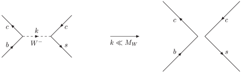
FIG. 1.: From the full to the effective theory

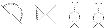
FIG. 2.: Diagrams contributing to the 1-loop mixing of the four-fermion operators.

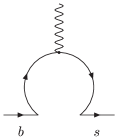
FIG. 3.: Diagram that gives finite contributions.

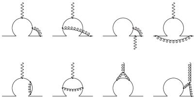
FIG. 4.: Two-loop diagrams needed for calculating the $\gamma$-matrix. The wavy line can be a photon or a gluon. These diagrams have no closed fermion loop.

FIG. 5.: Two-loop diagrams needed for calculating the $\gamma$-matrix. The wavy line can be a photon or a gluon. These diagrams have a closed fermion loop.

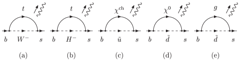
FIG. 6.: Diagrams that contribute to the matching of $O_{7/8}$ and $\tilde{O}_{7/8}$. The outgoing photon/gluon is attached at every possible position.

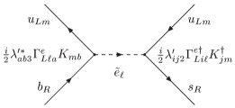
FIG. 7.: Illustration of the example in equation (85).

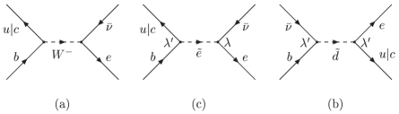
FIG. 8.: Contributions to $b\rightarrow u|c\;e\bar{\nu}$. The arrows indicate the particle flow.

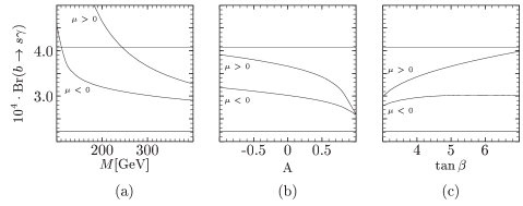
FIG. 9.: Behaviour of Br$(b\rightarrow s\gamma)$ in the neighbourhood of our reference model with $\tan\beta=5$, $A=0$, $\tilde{\mu}_{2i}=0$, $M=300$ GeV and, in addition, $\lambda^{\prime}_{132}=\lambda^{\prime}_{122}=0.1$. The horizontal lines show the current experimental bounds.

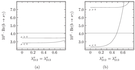
FIG. 10.: Values for Br$(b\rightarrow s\gamma)$ as a function of $\lambda^{\prime\prime}_{212}=\lambda^{\prime\prime}_{213}$. The other parameters are: $\tan\beta=5$, $A=0$, $\tilde{\mu}_{2i}=0$, and (a): $M=300$ GeV, (b): $M=100$ GeV. The current bounds are: $\lambda^{\prime\prime}_{212}\leq 1.23$, $\lambda^{\prime\prime}_{213}\leq 1.23$ [11], $|\lambda^{\prime\prime}_{212}\cdot\lambda^{\prime\prime}_{213}|\leq 0.006$ [12].

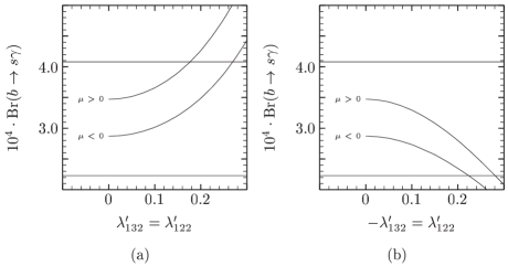
FIG. 11.: Values for Br$(b\rightarrow s\gamma)$ as a function of (a) $\lambda^{\prime}_{132}=\lambda^{\prime}_{122}$, (b) $-\lambda^{\prime}_{132}=\lambda^{\prime}_{122}$. The current bounds are: $\lambda^{\prime}_{132}\leq 0.28\frac{m_{\tilde{t}}}{100\mathrm{GeV}}$, $\lambda^{\prime}_{122}\leq 0.049\frac{m_{\tilde{d}}}{100\mathrm{GeV}}$ [11].

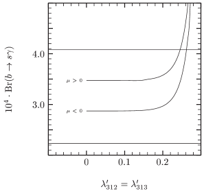
FIG. 12.: Values for Br$(b\rightarrow s\gamma)$ as a function of $\lambda^{\prime}_{312}=\lambda^{\prime}_{313}$ within our reference model. The current bounds are: $\lambda^{\prime}_{312}\leq 0.11\frac{m_{\tilde{s}}}{100\mathrm{GeV}}$, $\lambda^{\prime}_{313}\leq 0.11\frac{m_{\tilde{b}}}{100\mathrm{GeV}}$ [11], $|\lambda^{\prime}_{312}\cdot\lambda^{\prime}_{313}|\leq 0.01$ for squarks of 100 GeV [13]. The peak results from a small lightest selectron mass.

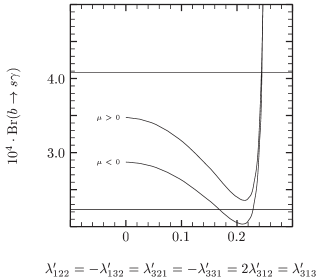
FIG. 13.: Values for Br$(b\rightarrow s\gamma)$ as a function of $-\lambda^{\prime}_{132}=\lambda^{\prime}_{122}=-\lambda^{\prime}_{331}=\lambda^{\prime}_{321}=2\lambda^{\prime}_{312}=\lambda^{\prime}_{313}$ within our reference model. Additional current bounds are: $\lambda^{\prime}_{331}\leq 0.45\frac{m_{\tilde{b}}}{100\mathrm{GeV}}$, $\lambda^{\prime}_{321}\leq 0.52\frac{m_{\tilde{d}}}{100\mathrm{GeV}}$ [11].

REFERENCES

- [1] S. Ahmet et al. eprint CLEO CONF 99-10.
- [2] A. Czarnecki and W. Marciano, Phys. Rev. Lett. 81, 277 (1998).
- [3] H. P. Nilles, Phys. Rep. 110, 1 (1984).
- [4] A. Smirnov and F. Vissani, Phys. Lett. B202, 138 (1988).
- [5] H. Dreiner eprint hep-ph/9707435.
- [6] H. Haber and G. Kane, Phys. Rep. 117, 75 (1985).
- [7] J. Gunion and H. Haber, Nucl. Phys. B272, 1 (1986).
- [8] S. Dawson eprint hep-ph/9712464.
- [9] A. Chamseddine and H. Dreiner, Nucl. Phys. B447, 195 (1995).
- [10] A. Chamseddine and H. Dreiner, Nucl. Phys. B458, 6 (1996).
- [11] B. Allanach et al. eprint hep-ph/9906224.
- [12] P. Roy eprint hep-ph/9712520.
- [13] G. Bhattacharyya eprint hep-ph/9709395.
- [14] K. Agashe and M. Graesser, Phys. Rev. D 54, 4445 (1996).
- [15] B. de Carlos and P. White, Phys. Rev. D 55, 4222 (1997).
- [16] G. Gamberini, G. Ridolfi, and F. Zwirner, Nucl. Phys. B 331, 331 (1990).
- [17] R. Arnowitt and P. Nath, Phys. Rev. D 46, 3981 (1992).
- [18] B. de Carlos and J. Casas, Phys. Lett. B 309, 320 (1993).
- [19] S. Coleman and E. Weinberg, Phys. Rev. D 7, 1888 (1973).
- [20] D. Guitsos eprint hep-ph/9905278.
- [21] A. Buras, hep-ph/9806471 An excellent detailed review on this topic.
- [22] B. Grinstein, R. Springer, and M. Wise, Phys. Lett. B 202, 138 (1988).
- [23] B. Grinstein, R. Springer, and M. Wise, Nucl. Phys. B 339, 269 (1990).
- [24] S. Herrlich and U. Nierse, Nucl. Phys. B 455, 39 (1995).
- [25] A. Buras and P. Weisz, Nucl. Phys. B 333, 66 (1990).
- [26] M. Ciuchini, E. Franco, L. Reina, and L. Silvestrini, Nucl. Phys. B 421, 41 (1994).
- [27] M. Ciuchini, E. Franco, G. Martinelli, L. Reina, and L. Silvestrini, Phys. Lett. B 316, 127 (1993).
- [28] M. Misiak, Phys. Lett. B 269, 161 (1991).
- [29] M. Misiak, Phys. Lett. B 321, 113 (1994).
- [30] M. Ciuchini, G. Degrassi, P. Gambino, and G. Giudice, Nucl. Phys. B 534, 3 (1998).
- [31] A. Ali and C. Greub, Z. Phys. C 49, 431 (1991).
- [32] A. Ali and C. Greub, Phys. Lett. B 259, 182 (1991).
- [33] A. Ali and C. Greub, Phys. Lett. B 361, 146 (1995).
- [34] C. Greub and T. Hurth, Phys. Rev. D 56, 2934 (1997).
- [35] C. Greub and T. Hurth p. 2934, eprint hep-ph/9708214.
- [36] C. Greub, T. Hurth, and D. Wyler, Phys. Lett. B 380, 385 (1996).
- [37] C. Greub, T. Hurth, and D. Wyler, Phys. Rev. D 54, 3350 (1996).
- [38] M. Misiak and M. Münz, Phys. Lett. B 344, 308 (1995).
- [39] K. Chetyrkin, M. Misiak, and M. Münz, Phys. Lett. B 400, 206 (1997).
- [40] K. Adel and Y. Yao, Mod. Phys. Lett. A 8, 1679 (1993).
- [41] K. Adel and Y. Yao, Phys. Rev. D 49, 4945 (1994).
- [42] G. Altarelli, G. Curci, G. Martinelli, and S. Petrarca, Nucl. Phys. B 187, 461 (1981).
- [43] A. Buras, A. Kwiatkowski, and N. Pott, Nucl. Phys. B 517, 353 (1998).
- [44] T. Inami and C. Lim, Prog. Theor. Phys. 65, 297 (1981).
- [45] S. Bertolini, F. Borzumati, A. Masiero, and G. Ridolfi, Nucl. Phys. B 353, 591 (1991).
- [46] F. Gilman and M. Wise, Phys. Rev. D 20, 2392 (1979).
- [47] K. Chetyrkin, M. Misiak, and M. Münz, Nucl. Phys. B 518, 473 (1998).
- [48] E. J. Chun, K. Hwang, and J. S. Lee eprint hep-ph/0005013.
- [49] A. Buras, M. Misiak, M. Münz, and S. Pokorski, Nucl. Phys. B 424, 374 (1994).
- [50] F. Borzumati and A. Masiero, Phys. Rev. Lett. 59, 180 (1987).
- [51] N. Cabibbo and L. Maiani, Phys. Lett. 79 B, 109 (1978).
- [52] J. Cortes, X. Pham, and A. Tounsi, Phys. Rev. D 25, 188 (1982).
- [53] G. Fogli, Phys. Rev. D 28, 1153 (1983).
- [54] C. Caso et al. (Particle Data Group), Europ. Phys. J. C 3, 1 (1998).
- [55] S. Wolfram, The Mathematica Book (Cambridge Univ. Press, Cambridge, 1999), 4th ed.
- [56] H. Baer, C. Chen, and R. Munroe, Phys. Rev. D 51, 1046 (1995).
- [57] H. Baer and M. Brhlik, Phys. Rev. D 55, 3201 (1997).
- [58] H. Baer, M. Brhlik, D. Castaño, and X. Tata, Phys. Rev. D 58, 015007 (1998).
- [59] B. de Carlos and J. A. Casas, Phys. Lett. B 349, 300 (1995), erratum ibid. B 351, 604 (1995).
- [60] B. de Carlos and P. White, Phys. Rev. D 54, 3427 (1996).
- [61] J.-P. Derendinger and C. Savoy, Nucl. Phys. B 237, 307 (1984).
- [62] B. Gato, J. León, J. Pérez-Mercader, and M. Quirós, Nucl. Phys. B 253, 285 (1985).
- [63] N. Falck, Z. Phys C 30, 247 (1986).