Edinburgh 2000/09
CERN-TH/2000-105
hep-ph/0004060
{centering}
STATIC CORRELATION LENGTHS IN QCD AT
HIGH TEMPERATURES AND FINITE DENSITIES
A. Harta, M. Laineb,c and O. Philipsenb
aDept. of Physics and Astronomy, Univ. of Edinburgh,
Edinburgh EH9 3JZ, Scotland, UK
bTheory Division, CERN, CH-1211 Geneva 23,
Switzerland
cDept. of Physics, P.O.Box 9, FIN-00014 Univ. of Helsinki,
Finland
Abstract
We use a perturbatively derived effective field theory and three-dimensional lattice simulations to determine the longest static correlation lengths in the deconfined QCD plasma phase at high temperatures () and finite densities (). For vanishing chemical potential, we refine a previous determination of the Debye screening length, and determine the dependence of different correlation lengths on the number of massless flavours as well as on the number of colours. For non-vanishing but small chemical potential, the existence of Debye screening allows us to carry out simulations corresponding to the full QCD with two (or three) massless dynamical flavours, in spite of a complex action. We investigate how the correlation lengths in the different quantum number channels change as the chemical potential is switched on.
Edinburgh 2000/09
CERN-TH/2000-105
May 2000
1 Introduction
With the advent of RHIC and ALICE, there is a growing need for a precise understanding of various properties of QCD at temperatures up to a GeV. At the moment, we are still far from a satisfactory level in this respect, even for the equilibrium properties of the plasma. Indeed, even though the system can in principle be described as a gas of quarks and gluons, a fully perturbative computation with these degrees of freedom does in practice not work well at any reasonable temperatures below GeV, since the perturbative series is badly convergent due to infrared sensitive contributions [1]–[4]. On the other hand, the only systematic fully non-perturbative method available, four-dimensional (4d) lattice simulations, is severely restricted in the presence of light dynamical fermions, and even more so in the presence of a finite baryon density; the current state of the art is summarised in [5]. A first principles solution of any problem related to non-equilibrium phenomena remains even further in the future.
The physics problem we address in this paper is the determination of various static correlation lengths. To tackle this problem, we will employ a method which can overcome some of the difficulties mentioned above. The method combines analytic and numerical techniques, in a way that both are used in a regime where they are well manageable. First, perturbation theory is employed in deriving, by what is called dimensional reduction [6, 7, 8, 9, 3, 4], an effective theory for the long range degrees of freedom of the system. At high temperatures all such degrees of freedom are bosonic, since fermions are screened by non-zero Matsubara frequencies , with odd. The reduction step can thus be carried out with dynamical, massless fermions and, as we shall see, with a finite chemical potential. Second, non-perturbative lattice simulations are used to study the infrared sensitive dynamics of the remaining degrees of freedom. The theory to be studied with simulations is the SU(3)+adjoint Higgs model in three dimensions (3d), and many of its properties have already been determined [10].
The method we employ suffers clearly from a number of restrictions. First of all, in QCD it is limited to temperatures above , roughly 111For the electroweak theory, in contrast, similar methods allow for a precise determination of the properties of the phase transition at for Higgs masses GeV [11, 12].. This can be inferred from a comparison of the dynamical scales described by the effective theory to those integrated out [4] as well as, more concretely, from a direct quantitative comparison of the correlation lengths measured within 3d for SU(2) [13], with those determined using 4d SU(2) lattice simulations at finite temperature (without fermions) [14]222For early work with similar conclusions both in SU(2) and SU(3), see [7]. Recently, analogous results have been reached also by considering gauge fixed correlators [15], as well as by considering dimensional reduction of pure SU(3) from (2+1)d to 2d [16].. Second, as we shall see, it is also limited by the largest chemical potential that can be reached. We will be able to go up to .
If there are restrictions, there are also strengths. What can be done within the effective theory can be done quite precisely. The simulations are comparatively easy technically, they yield high accuracy continuum limits for the quantities under investigation, and hence there is little ambiguity in the conclusions. For instance, studies in 3d have produced detailed and accurate insight into the relative sizes of perturbative and non-perturbative contributions to the Debye screening length [17, 13], a quantity which could be directly relevant for such signals of the quark–gluon plasma as suppression.
In the present work, we extend the study of [13] first to SU(3) Yang-Mills theory, and then to two- and three-flavour QCD in the massless limit. In comparing with earlier results in SU(3) [4, 17], we improve on the accuracy of Debye screening length determination and measure the screening lengths also in the other quantum number channels. We also discuss explicitly the and dependence of our results — here is the number of colours and is the number of (massless) quark flavours.
We then proceed to extend our calculations to finite baryon density. Our approach is straightforward: dimensional reduction leads to an additional complex term in the effective action, which has to be absorbed in the observables for practical simulations. This “reweighting” displays in principle similar problems as chemical potential simulations in four dimensions (for reviews, see [5, 18]). We find that for the effective theory there exists a range of volumes and ratios , however, for which the problems are in practice manageable. We demonstrate this by investigating a range of imaginary chemical potentials [19], for which we find complete agreement between reweighted calculations and those using the exact action. We then employ the reweighting technique to the case of real chemical potentials.
2 Continuum formulation for
We start by reviewing the result of the dimensional reduction step for . We follow closely Ref. [4].
The effective theory emerging from hot QCD by dimensional reduction [6] is the SU(3)+adjoint Higgs model with the action
| (2.1) |
where , , , and are all traceless Hermitian matrices (, etc), and and are the gauge and scalar coupling constants with mass dimension one, respectively. The physical properties of the effective theory are determined by the two dimensionless ratios
| (2.2) |
where is the dimensional regularization scale in 3d. The parameters , as well as the scale , are via dimensional reduction functions of the temperature and the QCD scale . For , the result is [4]
| (2.3) | |||||
| (2.4) | |||||
| (2.5) |
We have assumed here massless flavours, but the inclusion of quark masses is also possible in principle.
The scales entering in Eqs. (2.3), (2.4) are
| (2.6) | |||||
| (2.7) | |||||
| (2.8) |
To be explicit, for we obtain
| (2.9) |
Corrections to these expressions are of relative magnitude .
An important question is how small one can in practice take and still have only small corrections in Eqs. (2.3)–(2.5). As was observed in [4], for the expansion appears to converge surprisingly fast, with an error on a few percent level even at . The expansions need a priori not be as good for every parameter, however.
Consider for instance . One may expect higher loop graphs to amount to an increase in the effective scale factor , since there are many “massive” () particles inside the loops instead of one. Thus an upper bound on the error in can be obtained by evaluating the 2-loop QCD running coupling at the 1-loop scale (for ). This gives a correction of up to 25%, which is quite large. An explicit computation of including effects of order would thus be welcome in order to clarify whether the expansion for in reality converges as rapidly as for or not. Such computations are beyond our scope here and we will simply use Eqs. (2.3)–(2.5); a comparison with direct 4d simulations at turns out to be quite satisfactory within this procedure, and thus we will work under the assumption that the error in is similarly small as in .
Finally, we may sometimes want to express the temperature to which our simulations correspond in terms of , rather than . In view of Eq. (2.9), this requires knowledge of the deconfinement temperature , which can only be fixed with 4d simulations. For the case , we take the value from [22]333A recent computation [23] favours a slightly larger central value, but well within the error bars.. For , the determination of is not accurate, and we will take as a reference. Our results however only depend on , so they can be reinterpreted as corresponding to some other temperature relative to if need be.
2.1 Operators and quantum numbers
The physical observables on which we shall focus in this paper are spatial correlation lengths of QCD at finite temperatures. For the practical calculations we reinterpret the 3d theory in Eq. (2.1) which we use to compute them, as a (2+1)d one. We take operators to live on the ()-plane, and the correlations are taken in the direction. Thus we compute the spectrum of the 2d Hamiltonian of the effective theory, whose eigenvalues then correspond to screening masses or inverse spatial correlation lengths of the 4d theory at finite temperature. Thus, unless otherwise stated, “bound states”, “glueballs” etc. refer to the eigenstates of the effective Hamiltonian and to the screening masses of the 4d theory in the above sense.
We use the quantum number notation
| (2.10) | |||||
| (2.11) | |||||
| (2.12) |
The action in Eq. (2.1) is invariant under these operations. In the finite temperature context, the operation in the 3d theory is a remnant of the 4d time reversal operation [24]. The parity means a parity on the 2d plane, i.e. a reflection across the -axis. The charge conjugation is a non-trivial quantum number only for SU(3), since for SU(2) it is just a global gauge transformation , so that there are no gauge invariant operators odd in [24]. In addition to these discrete transformations, we define a rotation in the ()-plane, with the corresponding angular momentum . Thus the full symmetry group is , and accordingly we classify our operators and states by .
We note from Eqs. (2.10)–(2.12) that apart from , the action of on the operators in the ()-plane corresponds to complex conjugation (and ). Thus any real operator which does not contain is even in . This means, in particular, that for the scalar operators in which no single can appear, there are effectively only two quantum numbers left out of the original three, thus four different channels. The lowest dimensional gauge invariant operators of these types in the channels are:
| (2.13) |
All operators here with vanish identically for SU(2). Going out of the plane (i.e., allowing also for ), other channels would in principle become possible [24], but we do not expect them to change our conclusions.
3 Lattice formulation for
To simulate the effective theory in Eq. (2.1) on the lattice, we use the discretised version
| (3.1) | |||||
where the fields in the lattice action have been rescaled relative to the continuum, where is the lattice spacing, and denotes the elementary plaquette in the -plane located at . The parameters of the continuum and lattice theory are up to two loops related by a set of equations which become exact in the continuum limit [25, 26],
| (3.2) | |||||
For a given pair of continuum parameters these equations determine the lattice parameters as a function of the lattice spacing, and hence govern the approach to the continuum limit, . We have not implemented improvement [27] here, since the discretisation effects in the correlation lengths are already quite small at the values of we are using.
3.1 Observables
Operators for all the quantum number channels considered can be constructed from a number of basic operator types. We consider operators involving only scalar fields or products of scalar and gauge field variables,
| (3.3) |
Furthermore, we have loop operators constructed from link variables only,
| (3.4) |
and in addition to the elementary plaquette , we also consider squares of size as well as rectangles of size , , . Another useful pure gauge operator is the Polyakov loop along a spatial direction ,
| (3.5) |
which can be used to extract the 3d string tension. It also gives useful information about finite volume effects via so called torelon states [28, 29].
Operators with definite quantum number assignments are constructed from the above types by taking linear combinations with appropriate transformation properties. Clearly operators containing an even number of scalar fields, such as , will couple to states, and those with odd, such as , to . The different channels can be chosen by utilising the projection operators , where, e.g., , . Different spin states are obtained by employing the operation which rotates the operators by around . Note also that even though lattice rotations are restricted to multiples of , we are in practice close enough to the continuum limit that continuum symmetries are reproduced within the statistical errors; thus we keep the continuum notation in terms of even on the lattice.
In the following we list the operators used corresponding to Eq. (2.13):
| channel: | ||
| : | , | |
| : | , | |
| : | real part of symmetric combinations of , | |
| : | , | |
| : | , | |
| channel: | ||
| : | imaginary part of symmetric combinations of , | |
| : | , | |
| channel: | ||
| : | , | |
| channel: | ||
| : | , | |
| : | . |
We have also measured higher spin states. For we have a fairly large basis, identical to the one described in [13]. The states prove to be quite heavy, so that their relevance for the 4d finite temperature system is not immediately obvious at modest temperatures, and thus for simplicity we consider here only the ground states in the channels with , without specifying the other quantum numbers.
3.2 Blocking and matrix correlators
For later reference, let us recall the general principles of how the operators discussed above can be used for a reliable extraction of correlation lengths [30].
The eigenstates of the 2d Hamiltonian in the region of parameter space where we work are bound states. In order to increase the overlap of our operators onto such extended states, we construct smeared link and scalar field variables as described in [13]. For every quantum number channel, we then measure the correlation matrix
| (3.6) |
where we have denoted . This matrix can be diagonalised by solving a generalised eigenvalue problem,
| (3.7) |
where . We carry out this procedure at which gives somewhat differing eigenvectors , and check that the final outcome remains the same within error bars. We normalise the eigenvectors according to , so that satisfy , and are thus the normalized eigenstates of the 2d Hamiltonian. The final results are extracted from the correlation functions
| (3.8) |
by computing effective masses
| (3.9) |
and ensuring that these have attained a stable plateau value. Information about the composition of in terms of the operators used in the simulation, which we shall quote in some of our tables, is obtained from the overlaps .
3.3 Simulation and analysis
In our Monte Carlo simulation of the lattice action, Eq. (3.1), link variables are updated by a combination of heat bath and over-relaxation steps with algorithms described in [31]. The scalar fields are generated by a combination of heat bath and reflection steps [32]. One “compound” sweep consists of several over-relaxation and reflection updates following each heat bath update of gauge and scalar fields. Measurements are taken after every compound sweep. Typically, we gathered between 5 000 and 20 000 measurements depending on the lattice sizes. Statistical errors are estimated using a jackknife procedure with bin sizes of 100 – 250 measurements.
4 Numerical results for
In this section we discuss simulations of the effective theory for parameter values corresponding to hot SU(3) gauge theory with flavours of fermions at zero baryon density. Detailed investigations of finite volume effects and scaling of correlation lengths have been performed for the 3d pure SU(2) and SU(2)+adjoint Higgs theories in [31, 13], as well as for the 3d pure SU(3) theory in [31, 17]. In these works explicit continuum extrapolations were performed. For large enough the scaling behaviour was found to be quite good, with continuum results differing from those on a fine lattice by only a few percent. Our gauge couplings here were chosen to produce a similar lattice spacing, and checks also show good scaling. The parameter combinations and the lattices used for them are collected in Table 1.
| 2. | 0 | 0. | 11346 | 0. | 39188 | , | ||
| 0. | 009636 | 4. | 0 | — | ||||
| 1. | 5 | 0. | 10304 | 0. | 43668 | — | ||
| 2. | 0 | 0. | 09191 | 0. | 4830 | |||
| 1. | 5 | 0. | 08680 | 0. | 47890 | — | ||
| 2. | 0 | 0. | 07814 | 0. | 52741 | — | ||
| 2. | 0 | 0. | 062921 | 0. | 569680 | — | ||
4.1 The mass spectrum for
The main features of the spectrum, displayed in detail in Tables 5, 7 in the Appendix, are the same as those found in previous studies of the confinement region for SU(2) with fundamental [29] or adjoint [13] scalar fields. There is a dense spectrum of bound states, consisting of a replication of the glueball spectrum found in the pure SU(3) theory [31], and additional bound states of scalars, with little mixing between the two. This may be concluded from the fact that, as indicated in Table 5, some eigenstates are composed predominantly of purely gluonic operators , with practically no contribution from operators carrying the same quantum numbers but containing scalars. Comparing with [31], we find that our gluonic states have quantitatively the same masses as the corresponding glueballs in the pure Yang-Mills theory; the comparison is shown in Table 2.
| gauge–Higgs | pure gauge | |||||
| scalar | glueball | glueball | ||||
| 0. | 994 (19) | 2. | 511 (65) | 2. | 575 (18) | |
| 2. | 95 (16) | 3. | 61 (32) | 3. | 841 (28) | |
| 2. | 46 (10) | 3. | 50 (25) | 3. | 795 (27) | |
| 3. | 355 (94) | 4. | 14 (28) | 4. | 257 (33) | |
As can be observed from Table 2, however, in the physically interesting region of couplings the lightest states in given quantum number channels are not glueballs but always states including the scalar field . This can be understood in the sense that in the finite temperature context the phase transition is (for ) assumed to be driven by the symmetry related to (or on the lattice), and thus is the dominant infrared degree of freedom. Let us now discuss the corresponding correlation lengths in more detail.
4.1.1 The “magnetic” sector,
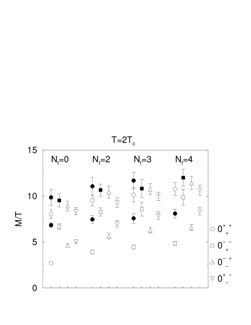
Consider first operators with . We will call this the “magnetic” sector, even though the operators can include an even number of -fields. This sector determines the correlation length related to the lowest lying glueballs and all other observables, as well as that felt by the real part of the 4d temporal Polyakov loop [33, 24] (not to be confused with the spatial Polyakov loop in the 3d theory). In order to express the masses in units of temperature, we use the perturbative expression for the gauge coupling in Eq. (2.3) to arrive at and . The spectrum in these units is shown in Fig. 1.
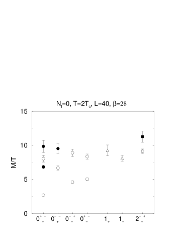
Let us first discuss the channel . From Table 5 in the Appendix, we note that the lightest state (open circle in Fig. 1(left)) is dominantly , while the next state (filled circle in Fig. 1(left)) is dominantly . Thus, the naïve ordering of states consisting of the fields and is reversed non-perturbatively: at low temperatures it is the which is responsible for the lightest gauge invariant state in the system.
As the temperature is increased, however, the ordering gets changed. The lowest state becomes heavier with increasing temperature, as the scalar “constituent mass parameter” is then growing (for a discussion of the constituent picture in a similar context, see [34, 15]). On the other hand, the glueball does not contain much admixture. Correspondingly its mass, in units of , is quite insensitive to , so that for large enough temperatures indeed the glueball corresponds to the lightest excitation. This situation is, however, only realised at high temperatures ; an extreme example is shown in Fig. 1(right). In this limit the may be integrated out, leaving the 3d pure SU(3) gauge theory as an effective theory [6].
For the channel , the behaviour is similar, but the masses are much larger. Let us mention here already that in the 4d theory with fermions at modest temperatures , all the higher-lying bosonic states in general are probably heavier than some gauge invariant states consisting of fermionic fields , which are not addressed by our theory, and whose mass we may expect to be . (At lower temperatures such states can be even lighter, since in the chiral limit they are expected to represent the critical degrees of freedom.)
To get an impression of the quality of dimensional reduction for , we now compare the state with that found directly from a 4d simulation at [14]. Our value is , to be compared with reported in [14]. In complete analogy with the SU(2) case [13], it is thus found that dimensional reduction quantitatively reproduces the lowest screening mass of the 4d Yang-Mills theory at temperatures as low as .
We can also carry out another comparison. The real part of the 4d temporal Polyakov loop carries quantum numbers , and non-perturbatively mixes with other operators in that channel. Correspondingly, its decay should also be determined by the bound state . Indeed, the exponential decay of the 4d temporal Polyakov loop correlator is in 4d measured to be [35], which is quite compatible with the value we find here.
On the other hand, in contrast to SU(2) where even several excitations agree between the full and the effective theory, we find here deviations of about 20% in comparing with [14]. This may signal that the effective theory is not as reliable for states whose mass is approaching . However, we also believe that there could be some room for improvement upon this apparent disagreement. The 4d simulations are quite difficult, and it is not easy to guarantee at this stage that the infinite volume and continuum limits are reached for the excited states.
4.1.2 The “electric” Debye sector,
Of particular phenomenological relevance for the QCD plasma is the Debye mass, whose inverse gives the length scale over which the colour-electric field is screened. The expansion in powers of coupling constants for this quantity reads
| (4.1) |
The perturbative leading order result is [36]
| (4.2) |
but at next-to-leading order , only a logarithm can be extracted [37] (the 2nd term on the right hand side of Eq. (4.1)), whereas the coefficient is entirely non-perturbative. To determine it, we use the gauge invariant definition of the Debye mass based on the Euclidean time reflection symmetry as given in [24]. According to this definition, the Debye mass corresponds to the mass of the lightest state odd under this transformation. The remnant of Euclidean time reflection symmetry in our reduced model is the scalar reflection symmetry , and the Debye mass thus corresponds to the mass of the lightest state of our spectrum. As shown in Fig. 1, this is the ground state , while is slightly heavier.
With this definition, the coefficient can be measured separately from the exponential decay of a Wilson line in a 3d pure gauge theory [24]. The measurements for have been performed in [17] with the results , . On the other hand, the mass we have measured here also includes the correction in Eq. (4.1). We can thus now estimate the magnitude of the remainder; our results are shown in Table 3. We find that the corrections are less than 30% even at temperatures as low as , and they disappear entirely for asymptotically large temperatures. The sign is negative, so that the complete result is somewhat smaller than estimated in [17] based on the perturbative contributions and alone, instead of . The result is also about % smaller than what can be extracted from [4], a difference which we presume to be due to the relatively small lattice sizes used there.
| pert. part | ||||||||||
|---|---|---|---|---|---|---|---|---|---|---|
| 1. | 70(5) | 0. | 514 | 1. | 65(6) | -0. | 46(6) | 4. | 6(2) | |
| 3. | 82(12) | 2. | 165 | 1. | 65(6) | 0. | 00(12) | 0. | 96(3) | |
We can conclude that for temperatures of physical interest, the Debye mass according to this definition is entirely non-perturbative, with its next-to-leading order correction being larger than the leading term. This remains to be the case up to [17]. But even at , as the table shows, there are sizeable corrections to the leading behaviour. This leads to the conclusion that the scale dominating the Debye mass is with non-perturbative physics for all temperatures of interest, in contrast to the naïve expectation . The reason for this behaviour is the large non-perturbative coefficient that appears in front of the correction term in the series in .
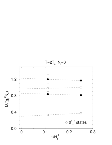
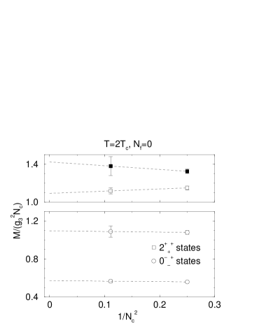
4.1.3 scaling between SU(2) and SU(3)
Let us finally discuss the scaling with . In [31] it was found for SU() pure gauge theories with that the differences in the mass spectra can be accounted for by the leading order corrections in a large expansion, and that the coefficients of these are remarkably small. In theories with various scalar fields, the glueball content has been found to be practically identical to that of pure gauge theories for [29, 38, 13], and thus the scaling behaviour with is preserved. It is then natural to ask if the same scaling behaviour holds for the scalar bound states, which are not present in the Yang-Mills theory. In Fig. 2 we plot some of our low lying states from the current analysis as well as the SU(2) case [13] (we have to focus on states with in order to have an SU(2) counterpart). Indeed we observe a similar scaling for the scalar states as for the glueballs. This suggests that the screening masses of hot SU(3) gauge theory are close to the limit, and hence large methods may be useful approximations to analytically deal with some of the non-perturbative aspects discussed here.
4.2 The mass spectrum for
Having convinced ourselves that dimensional reduction of pure Yang-Mills theory works at the very least for the lowest static bosonic correlation functions of the theory, we may now move ahead to exploit the advantage of this formalism, the easy inclusion of fermions. For the case of massless fermion, all that is required is to evaluate Eqs. (2.3)–(2.5) for the desired and simulate the effective theory with the corresponding parameters. Each of these simulations gives results completely analogous to those of the case, except for a slight shift in the values. For the reader interested in the detailed numbers, we collect our data in Tables 6, 8 in the Appendix, at temperatures , and , which probes the lower limit of the range of validity of dimensional reduction.
With the tables at hand, the spectrum shown in Fig. 1 for is now also known for . In Fig. 3 we display the dependence on of the low lying states. The general behaviour of slightly rising mass values with can be understood from Eqs. (4.1), (4.2). Increasing increases the value of corresponding to the bare scalar mass, and hence the masses of the bound states increase as well. In units of the temperature, the increase from to the phenomenologically interesting case is about 30% for , % for the other channels. The correlation lengths decrease accordingly.
4.3 The spatial string tension
Finally, let us discuss one observable of the 3d theory which does not have an interpretation as a physical 4d correlation length. A Polyakov loop in a spatial direction couples to a flux loop state (or torelon) that winds around the periodic boundaries of the finite volume. The exponential fall-off of its correlator is related to the mass of the flux loop, according to
| (4.3) |
Such a flux loop state can be easily identified through its energy scaling linearly with the size of the lattice as seen in, e.g., Table 9. Since the scalar fields are in the adjoint representation, they cannot screen the colour flux represented by the Polyakov loop in fundamental representation, in contrast to the case with fundamental scalars [39]. Thus, a string tension can be defined by the slope of the static potential at infinite separation, just as in pure gauge theory. Accordingly, the coefficient corresponds to the string tension at separation . For large enough , an estimate for the string tension in infinite volume is then provided by the relation [40]
| (4.4) |
We have extracted the string tension by diagonalising a basis of various smeared Polyakov loops, and the results are given in Tables 9, 10.
We note that the string tension in continuum units is rather insensitive to the precise parameter values , as it fluctuates by less than 4% between the cases considered. Moreover, all values are similarly close to the ones obtained in pure gauge theory [31]. This is a further indication of the insensitivity of the pure gauge sector to the presence of the adjoint scalar fields. In the context of Yang-Mills theory at finite temperature, the string tension of the effective theory corresponds to the spatial string tension as measured in 4d simulations at finite temperature. Indeed, our value on the finest lattice for , is in good agreement with the spatial 4d result given in [41].
5 Extension of the method to finite density
As we have mentioned in the Introduction, there is no satisfactory algorithm to simulate lattice QCD in four dimensions at finite baryon density, with small quark masses. On the other hand, in the experimental situation of heavy ion collisions there always is a net baryon density, which in the collisions at and above AGS and SPS energies can be estimated to correspond to [42]. As long as the temperature is sufficiently above , dimensional reduction is applicable for the lowest lying static correlation functions in QCD, as we have seen in the previous sections. We now proceed to dimensionally reduce QCD at finite temperature and density. As we shall see, it is possible to perform simulations in the -range of interest in this framework.
5.1 The effective theory with
At leading order, the introduction of leads to a very simple modification of the effective 3d theory in Eq. (2.1). New effects come only from fermions, where we change in the loop momenta; here denotes the fermionic Matsubara frequencies. The 1-loop effective potential computed in [43] tells then that the effective action for the Matsubara zero mode of has for the terms ()
| (5.1) |
There is of course no term linear in , unlike in the Abelian case [44]. Note furthermore that for SU(2), .
In general, the inclusion of also leads to other new operators than . However, as can be seen from the effective potential computed in [43], there are no higher order operators involving only , at least at 1-loop and 2-loop levels. On the contrary, there could be operators such as . As is usual in effective field theories, we expect such non-renormalizable operators to give contributions suppressed with respect to the dynamical effects arising within the effective theory in Eq. (5.1) by a power of the scale hierarchy, and therefore we ignore them here. It is perhaps also worthwhile to mention that since no appears in perturbation theory in QCD and since the construction of the effective theory in Eq. (5.1) is only sensitive to the ultraviolet and thus purely perturbative, no Chern-Simons type operators are expected to be generated.
Going to 3d units (, ) and denoting
| (5.2) |
the dominant changes due to in the action in Eq. (2.1) are then
| (5.3) |
Thus, one new operator is generated in the effective action, and one of the parameters which already existed, gets modified. We note that the new operator is quite special and it, for instance, does not generate new ultraviolet divergences for the parameters in the original action in Eq. (2.1).
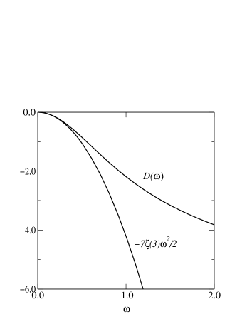
A more precise computation of the effective action requires the inclusion of 2-loop effects in Eq. (5.1), as well as a 1-loop computation of the wave function corrections of and the gauge coupling . We proceed as explained in [4], changing in the fermion propagators, and including the 2-loop contributions into the effective potential from [43, 45]. Let
| (5.4) | |||||
At small , . We then obtain
| (5.5) | |||||
| (5.6) | |||||
| (5.9) |
In the case we actually study, , these reduce to
| (5.10) | |||||
| (5.11) | |||||
| (5.12) | |||||
| (5.13) |
where , are from Eq. (2.9), and corrections are of relative order . Let us recall that at .
Due to the small value of , we will in the analysis which follows for simplicity ignore even the corrections in in Eqs. (5.10), (5.11), (5.13), and use the leading order expressions displayed already in Eq. (5.3). All of the sub-dominant effects neglected work in the same direction and would strengthen the changes we see in the mass spectrum. For this is obvious because, according to Eq. (5.13), for a given the physical value would be larger than what we have used. For , Eq. (5.11) and the negative value of imply that the fact that we have kept unchanged means that we have effectively moved slightly up in . In a major part of this effect cancels since the correction is the same in Eqs. (5.10), (5.11). Therefore, remains essentially the same for given , even though the temperature is slightly higher.
5.2 A complex action and reweighting
The generic problem of SU(3) simulations at non-vanishing chemical potential now appears as follows. For , there is the imaginary term in the action, and the conventional importance sampling will not work444It can be seen directly in 4d that the sign problem is strongly correlated with the imaginary part of the temporal Polyakov loop [21]. This corresponds precisely to in the 3d language.. A way to circumvent this is to do the importance sampling with the action at , while is included in the operators. We will refer to this procedure as “reweighting”. Reweighting is also applied in the “Glasgow method” suggested for simulations in 4d (for a review, see [46]); however, in our approach we do not need to carry out any expansion related to . Denoting by brackets the expectation value with respect to the action in Eq. (3.1), operators even and odd in therefore appear as
| (5.14) |
Since Eq. (5.14) involves trigonometric functions, the problem manifests itself if configurations with occur frequently. In this case there are cancellations in the functional integral, and the Monte Carlo method will soon lose its accuracy.
Configurations with need not always be typical, however. Indeed, let us consider the distribution of in Eq. (5.2) for . The centre of the distribution is at zero. The fact that there is Debye screening, , guarantees that the distribution is approximately Gaussian. Its width is easily computed, and is given by the 2-loop scalar sunset graph on the lattice, which has been evaluated in [25, 26]:
| (5.15) |
We note that the width grows with the lattice size (or, more precisely, with the physical lattice size )555For a fixed physical lattice size, the width grows with , but only logarithmically.. Nevertheless, if is small enough, the infinite volume and continuum scaling limits of the correlation functions may be extracted before Eq. (5.15) grows to values . In these cases we can in practice carry out all the measurements before the oscillations set in. The feasibility of this procedure can be checked by monitoring the numerical distribution of , the argument of the reweighting factors. Accurate calculations should be possible whenever the bulk of the distribution is contained in the interval . Once the distribution gets significantly broader, the breakdown should show up in the correlation functions simply as a noisy signal.
Even assuming that the oscillations are under control, reweighting according to Eq. (5.14) of course requires some care. The importance sampling of the Monte Carlo is dominated by the minimum of the action at , which is unmodified by including in the operators. If the minimum is widely separated from the true minimum in configuration space, there is a danger of biasing the Monte Carlo towards the wrong configurations. In order to check this, we have tested the reweighting method by considering imaginary, . In this case the action is real and the scalar update can be modified by a Metropolis step to include , and hence update with the exact action. The results can then be compared with those obtained from Eq. (5.14), now with
| (5.16) |
Simultaneously, we change the sign of in in Eq. (5.3).
5.3 Determining masses with a complex action
Assuming that our reweighting procedure works, we then have to extract masses in the changed symmetry situation. After the inclusion of , the action of the effective theory is no longer real, and no longer invariant in . It is however still invariant under and . In the scalar channel this means that the operators and in Eq. (2.13) can couple to each other, and similarly and . These two channels are still distinguished, however, by the parity .
We measure the correlation matrix between the two channels which used to be decoupled for . From Eq. (5.14) we know that the result is of the block form
| (5.17) |
where , are symmetric matrices (possibly of different sizes), representing the correlations within the two channels as in Eq. (3.6). We have factored out in the off-diagonal blocks, to make it clear that the result is odd in and vanishes for . In order to facilitate the solution of the eigenvalue problem in Eq. (3.7), we may note that we can equivalently consider the eigenvalue problem for the real correlation matrix
| (5.18) |
obtained from by a similarity transformation . Finally, for imaginary chemical potentials we have a correlation matrix of the usual symmetric form as in Eq. (3.6),
| (5.19) |
In addition, let us note that physical observables such as masses (i.e., inverse correlation lengths) must be even in , since a change of its sign can be compensated for by the field redefinition in the action in Eq. (5.3). Since the mass spectrum is well defined and there are no massless modes at , we moreover expect that the system is analytic in for small , the expressions of the masses starting with . In particular, masses must remain real for small enough (even though for the eigenvalues of a fully general matrix of the form in Eqs. (5.17), (5.18) this is not always the case).
We can use these observations to discuss the form of the mass eigenstates. For the cases in Eqs. (5.17), (5.18), we do not in general have orthonormal eigenvectors in the usual sense. In order for the procedure to make physical sense, we however expect (and observe) that the eigenvectors are independent of within statistical accuracy, with eigenvalues of the form , as in Eq. (3.7).
Consider now first Eq. (5.19). Since the eigenvalues are even in , the eigenvectors should be of the forms
| (5.20) |
where normalisation conditions have also been shown. With analytic continuation, we can then directly apply this to the case of Eq. (5.17),
| (5.21) |
as well as to the case of Eq. (5.18), using the similarity transformation:
| (5.22) |
We observe that the “metric” has changed, but otherwise the situation is quite analogous to the usual one in Eq. (5.20).
Fortunately, in practice even less needs to be changed in the usual numerical analysis based on a matrix of the form in Eqs. (3.6), (5.19), if we use Eq. (5.18). There are algorithms finding the eigenvalues and eigenvectors for a general non-symmetric real matrix. The only change is in the normalisation according to Eq. (5.22), which amounts to fixing an overall coefficient for each eigenvector. However, as we only consider the correlations between the eigenvectors, cf. Eq. (3.8), and do not need to verify orthogonality explicitly, we can equally well employ a “wrong” scalar product and normalisation based on the old type of metric in Eq. (5.20) (with ). Then everything goes precisely as before.
Finally, let us illustrate the general expectations for the mass pattern with a simple matrix as an analogue of Eq. (5.17). Consider two real scalar fields , with a mass term
| (5.23) |
For and , the mass eigenvalues are real, , . Thus the lightest mass goes up, which is what we expect for a real chemical potential. In fact there is another effect contributing in the same direction, since according to Eq. (5.3) the parameter grows with . In the case of a complex , on the contrary, the lightest mass becomes even lighter, the heaviest mass even heavier: , . Again, the change of contributes in the same direction for the lightest mass.
6 Numerical results for
We now proceed to present the results of our first numerical explorations of . We restrict our attention to the case , , corresponding to . As we have explicitly checked for good scaling behaviour at , we work exclusively with in this section. The parameters and lattices considered are summarised in Table 4, and the detailed results are displayed in Tables 11, 12 in the Appendix.
| 0. | 5 i | 0. | 47382 | 0. | 0338 i | |
| 1. | 0 i | 0. | 44630 | 0. | 0675 i | |
| 1. | 5 i | 0. | 40042 | 0. | 1013 i | |
| 0. | 5 | 0. | 49218 | 0. | 0338 | |
| 1. | 0 | 0. | 51970 | 0. | 0675 | |
| 1. | 5 | 0. | 56558 | 0. | 1013 | |
| 2. | 0 | 0. | 62981 | 0. | 1351 | |
| 4. | 0 | 1. | 07026 | 0. | 2702 | |
6.1 Consistency checks and the general pattern
We begin by assessing the distribution of the argument of the reweighting factors in Eq. (5.14). We find that any typical histogram can be easily fitted to a Gaussian, from which we determine its width. The plots in Fig. 5 show the corresponding distributions as a function of and the lattice volume, with behaviour as expected from Eq. (5.15). The volume chosen for the series is large enough to be free from finite size effects in the simulations. As the histograms show, for these volumes the distribution of the argument of the reweighting factor is entirely contained within one period for . On the other hand, at the tails of the distribution are significantly spreading. Nevertheless, the bulk of the distribution is still within the region without sign flips. For the same number of measurements at , however, the errors on the correlation functions are indeed by a factor of three larger in the latter case, confirming the onset of the sign problem. Going to still larger will thus lead to increasingly noisy signals, until a mass determination becomes impossible.


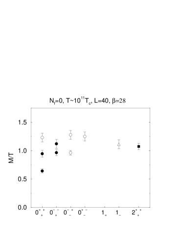
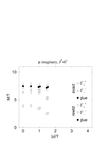
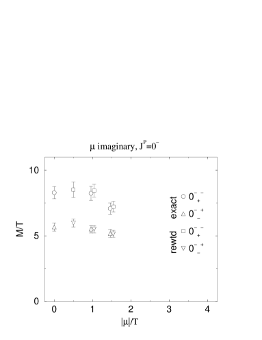
In the next step, we test the reliability of the reweighting procedure by comparing with the correct importance sampling in the case of an imaginary chemical potential. This comparison can only be carried out for a limited range of . In the full action, the imaginary chemical potential term weakens the metastability [4] of the symmetric phase, and tunnelling during typical simulations to the unphysical phase becomes possible. This can be countered by increasing the lattice volume, but in so doing we increase the width of the distribution of . We find however that there exists a window of opportunity between these two limits where we can usefully compare the two algorithms. In the left panels of Fig. 6, the ground states of the and channels are shown as a function of imaginary . First, we note the correct qualitative behaviour of a mass decrease with , as described after Eq. (5.23). Second, we observe complete agreement within the small statistical errors between the reweighted observables and those measured with the full action.
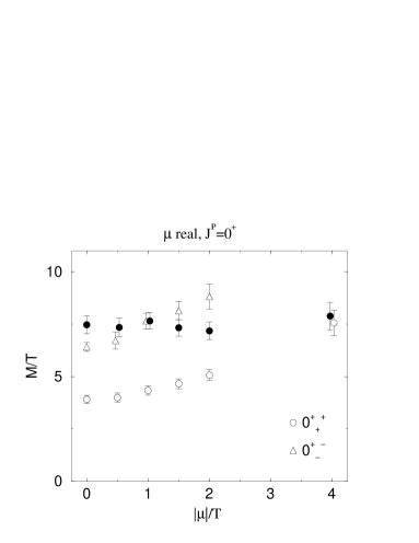
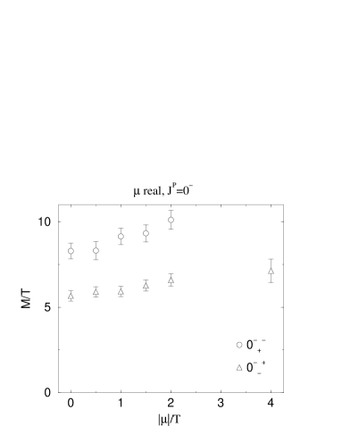
With these tests passed, we can thus display the same states for the case of real chemical potential in the right panels of Fig. 6. Again in agreement with the qualitative behaviour expected from the discussion after Eq. (5.23), the lowest mass values are growing with increasing , since the constituent mass parameter gets larger, see Eq. (5.3). Thus the corresponding correlation lengths decrease. We note again, however, that purely gluonic states (or, in the 4d language, purely magnetic states ) are rather insensitive to , in analogy with their behaviour under variations of discussed earlier. This means that at large enough , they may become the lightest states in the system, as suggested by the top right panel of Fig. 6.
At we have performed a finite volume check, comparing lattices of and at . We find the low lying masses to be consistent within statistical errors, see Table 12. This is encouraging, implying that the reweighting does not magnify finite volume effects unduly, and that it is indeed possible to extrapolate screening masses to the infinite volume in a finite chemical potential context, before the onset of oscillations.
6.2 The Debye screening length at finite baryon density
Let us now consider what happens to the Debye screening length as defined in Sec. 4.1.2. This definition is based on the -symmetry of our effective theory [24]. For the extra term in the action spoils the symmetry, resulting in a merging of the various -channels, while only remains as a good quantum number. The question then arises, how can the Debye mass be defined in such a situation [24]?
We now note the following. For , the lightest state was . This is, however, also the lightest state in the channel . Thus, even after , the same operator continues to determine the long distance decay of a number of operators. The values can be seen in Fig. 6, bottom right. If we define this largest correlation length to correspond to Debye screening, then does not change the situation in an essential way, and the corresponding correlation length decreases with . An example of a 4d gauge invariant operator with such a behaviour is [24].
On the other hand, the operator does couple to after the inclusion of . Therefore, its correlation length strictly speaking increases by a factor of almost two as soon as , as can be seen from the top right panel in Fig. 6. There we have labelled the states with the quantum numbers of the limit; however, for , any operator which originally had just the quantum numbers such as , couples now also to . The eigenstate shown in Fig. 6 which does have a larger mass, is a particular linear combination of the two types of original states. Nevertheless, the overlap between the two operators , is very small for small , so that even for there is an intermediate distance range where correlations should decay as shown with in Fig. 6, as discussed in [24]. Thus no abrupt change is observed. An example of a gauge invariant 4d operator with such a behaviour is the imaginary part of the 4d temporal Polyakov loop.
7 Conclusions
In this paper, we have carried out mass measurements in the different quantum number channels within the 3d SU(3)+adjoint Higgs theory. We have stayed on the dimensional reduction curve in the symmetry restored phase of the 3d theory, and the results are thus expected to correspond to spatial correlation lengths in the deconfined quark–gluon plasma phase of QCD. This interpretation appears to be relatively accurate at least down to . We first considered a vanishing chemical potential , and then also extended the measurements to a finite .
For , we believe that the asymptotic correlation lengths related to the real and imaginary parts of the 4d temporal Polyakov loop, as well as to other gauge invariant bosonic operators, are now relatively well understood. For instance, at , the real part of the Polyakov loop (with quantum numbers according to our conventions discussed in Sec. 2.1) decays exponentially at , while the imaginary part () decays at , as can be observed from Fig. 1. The Debye screening length according to the definition of [24] turns out to be determined by operators of the type , and is slightly longer than the screening length of the imaginary part of the Polyakov loop, .
We have also explicitly studied the effects of dynamical fermions on the longest correlation lengths. For fixed , the correlation lengths decrease as is increased. For instance, in the phenomenologically interesting case of at , the real part of the Polyakov loop decays exponentially at , while the imaginary part at . As a theoretical point, it is interesting to note that in units of , the screening lengths scale quite well with .
We have then extended the measurements to . We have demonstrated that the use of dimensional reduction allows one to carry out simulations corresponding to phenomenologically interesting values of quark masses, temperatures, and (although not at the point of the phase transition). Simulations are possible because the only term in the super-renormalizable 3d action suffering from the sign problem, , comes with a very small numerical coefficient.
In general, we observe that as is switched on at a fixed temperature, the screening lengths decrease. This can be interpreted so that the lightest excitations, involving , are “less critical” and correspondingly heavier. Thus, staying at a fixed temperature but increasing , we are apparently moving further away from the critical line, which hence has to bend down. This is in complete accordance with what we qualitatively know about the phase diagram in the -plane.
However, there is one state whose mass does not increase, the 3d glueball . Thus at large enough , similarly to the case of large enough at , it becomes the lightest excitation in the system. We find that the crossover corresponds roughly to in terms of the dimensionless parameter defined in Eqs. (2.2), (5.3). For , this corresponds roughly to at , and at .
Finally we have addressed the behaviour of the imaginary part of the 4d temporal Polyakov loop. As the chemical potential is switched on, its asymptotic correlation length suddenly increases contrary to the other observables discussed, and agrees for all with that of the real part of the 4d temporal Polyakov loop.
The task remains to establish a direct connection between the screening masses discussed here and observables relevant for the phenomenology of heavy ion collision experiments.
Acknowledgements
We acknowledge useful discussions with R.D. Pisarski and K. Rajagopal. This work was partly supported by the TMR network Finite Temperature Phase Transitions in Particle Physics, EU contract no. FMRX-CT97-0122. The work of A.H. was supported in part by UK PPARC grant PPA/G/0/1998/00621.
Note added
After the submission of our paper, a letter appeared by Gavai and Gupta [47], who measure the spatial meson (pion) correlation length at for light dynamical fermions. They observe that at the meson “mass” measured from has become lighter than the lightest bosonic mass (represented by in the 3d language), so that the bosonic gauge degrees of freedom are no longer the lightest dynamical degrees of freedom, and thus the standard dimensionally reduced effective theory should not be reliable any more. This observation is in accordance with our comments in Sec. 4.1.1. However, Gavai and Gupta make the further suggestion that even in the temperature range where the meson mass is no longer the lightest one, but is still below its asymptotic value ( in the case of the chiral continuum limit), dimensional reduction may not be reliable, in contrast to the situation in the purely bosonic case . Let us comment that there is no hard evidence for the latter suggestion. In fact, it seems quite possible to us that the decrease from could be partly accounted for precisely by the confining bosonic 3d gauge field dynamics related to . Furthermore, we see no evidence for why the bosonic correlation lengths we have measured here would not be satisfactorily reproduced by the 3d theory in this temperature range. Thus we believe that our bosonic mass measurement for (both at and ) do reproduce at least the qualitative features of the physical 4d theory at all temperatures .
As already discussed by Gavai and Gupta, one might also expect that chiral effects responsible for the behaviour seen by them are at somewhat larger than in the realistic case . For instance, is lighter for smaller as we have discussed in this paper, while still reaches the same asymptotic value, so that the level crossing invalidating dimensional reduction should take place at a smaller temperature.
References
- [1] A.D. Linde, Phys. Lett. B 96 (1980) 289; D.J. Gross, R.D. Pisarski and L.G. Yaffe, Rev. Mod. Phys. 53 (1981) 43.
- [2] P. Arnold and C. Zhai, Phys. Rev. D 50 (1994) 7603 [hep-ph/9408276]; Phys. Rev. D 51 (1995) 1906 [hep-ph/9410360].
- [3] E. Braaten and A. Nieto, Phys. Rev. Lett. 76 (1996) 1417 [hep-ph/9508406]; Phys. Rev. D 53 (1996) 3421 [hep-ph/9510408].
- [4] K. Kajantie et al, Nucl. Phys. B 503 (1997) 357 [hep-ph/9704416]; Phys. Rev. Lett. 79 (1997) 3130 [hep-ph/9708207].
- [5] F. Karsch, Plenary talk at Lattice ’99, hep-lat/9909006, to appear in the proceedings.
- [6] P. Ginsparg, Nucl. Phys. B 170 (1980) 388; T. Appelquist and R.D. Pisarski, Phys. Rev. D 23 (1981) 2305.
- [7] S. Nadkarni, Phys. Rev. Lett. 60 (1988) 491; T. Reisz, Z. Phys. C 53 (1992) 169; L. Kärkkäinen, P. Lacock, D.E. Miller, B. Petersson and T. Reisz, Phys. Lett. B 282 (1992) 121; Nucl. Phys. B 418 (1994) 3 [hep-lat/9310014]; L. Kärkkäinen, P. Lacock, B. Petersson and T. Reisz, Nucl. Phys. B 395 (1993) 733.
- [8] S. Huang and M. Lissia, Nucl. Phys. B 438 (1995) 54 [hep-ph/9411293]; Nucl. Phys. B 480 (1996) 623 [hep-ph/9511383].
- [9] K. Kajantie, M. Laine, K. Rummukainen and M. Shaposhnikov, Nucl. Phys. B 458 (1996) 90 [hep-ph/9508379]; Phys. Lett. B 423 (1998) 137 [hep-ph/9710538].
- [10] K. Kajantie, M. Laine, A. Rajantie, K. Rummukainen and M. Tsypin, JHEP 9811 (1998) 011 [hep-lat/9811004].
- [11] K. Kajantie et al, Nucl. Phys. B 466 (1996) 189 [hep-lat/9510020]; Nucl. Phys. B 493 (1997) 413 [hep-lat/9612006]; M. Gürtler et al, Nucl. Phys. B 483 (1997) 383 [hep-lat/9605042]; Phys. Rev. D 56 (1997) 3888 [hep-lat/9704013]; O. Philipsen et al, Nucl. Phys. B 528 (1998) 379 [hep-lat/9709145]; K. Rummukainen et al, Nucl. Phys. B 532 (1998) 283 [hep-lat/9805013].
- [12] F. Csikor, Z. Fodor and J. Heitger, Phys. Rev. Lett. 82 (1999) 21 [hep-ph/9809291]; M. Laine, JHEP 06 (1999) 020 [hep-ph/9903513].
- [13] A. Hart and O. Philipsen, Nucl. Phys. B 572 (2000) 243 [hep-lat/9908041].
- [14] S. Datta and S. Gupta, Nucl. Phys. B 534 (1998) 392 [hep-lat/9806034]; Phys. Lett. B 471 (2000) 382 [hep-lat/9906023].
- [15] F. Karsch, M. Oevers and P. Petreczky, Phys. Lett. B 442 (1998) 291 [hep-lat/9807035].
- [16] P. Bialas, A. Morel, B. Petersson, K. Petrov and T. Reisz, hep-lat/0003004.
- [17] M. Laine and O. Philipsen, Nucl. Phys. B 523 (1998) 267 [hep-lat/9711022]; Phys. Lett. B 459 (1999) 259 [hep-lat/9905004].
- [18] M. Alford, Nucl. Phys. B (Proc. Suppl.) 73 (1999) 161 [hep-lat/9809166].
- [19] M. Alford, A. Kapustin and F. Wilczek, Phys. Rev. D 59 (1999) 054502 [hep-lat/9807039]; M. Lombardo, hep-lat/9908006.
- [20] T.C. Blum, J.E. Hetrick and D. Toussaint, Phys. Rev. Lett. 76 (1996) 1019 [hep-lat/9509002]; R. Aloisio, V. Azcoiti, G. Di Carlo, A. Galante and A.F. Grillo, hep-lat/9903004; J. Engels, O. Kaczmarek, F. Karsch and E. Laermann, Nucl. Phys. B 558 (1999) 307 [hep-lat/9903030].
- [21] P. de Forcrand and V. Laliena, Phys. Rev. D 61 (2000) 034502 [hep-lat/9907004]; K. Langfeld and G. Shin, hep-lat/9907006.
- [22] J. Fingberg, U. Heller and F. Karsch, Nucl. Phys. B 392 (1993) 493.
- [23] B. Beinlich, F. Karsch, E. Laermann and A. Peikert, Eur. Phys. J. C 6 (1999) 133 [hep-lat/9707023].
- [24] P. Arnold and L.G. Yaffe, Phys. Rev. D 52 (1995) 7208 [hep-ph/9508280].
- [25] K. Farakos, K. Kajantie, K. Rummukainen and M. Shaposhnikov, Nucl. Phys. B 442 (1995) 317 [hep-lat/9412091].
- [26] M. Laine and A. Rajantie, Nucl. Phys. B 513 (1998) 471 [hep-lat/9705003].
- [27] G.D. Moore, Nucl. Phys. B 493 (1997) 439 [hep-lat/9610013]; Nucl. Phys. B 523 (1998) 569 [hep-lat/9709053].
- [28] C. Michael, J. Phys. G 13 (1987) 1001.
- [29] O. Philipsen, M. Teper and H. Wittig, Nucl. Phys. B 469 (1996) 445 [hep-lat/9602006]; Nucl. Phys. B 528 (1998) 379 [hep-lat/9709145].
- [30] G.C. Fox, R. Gupta, O. Martin and S. Otto, Nucl. Phys. B 205 (1982) 188; B. Berg and A. Billoire, Nucl. Phys. B 221 (1983) 109; M. Lüscher and U. Wolff, Nucl. Phys. B 339 (1990) 222; A.S. Kronfeld, Nucl. Phys. B (Proc. Suppl.) 17 (1990) 313.
- [31] M. Teper, Phys. Rev. D 59 (1999) 014512 [hep-lat/9804008].
- [32] B. Bunk, Nucl. Phys. B (Proc. Suppl.) 42 (1995) 566.
- [33] S. Nadkarni, Phys. Rev. D 33 (1986) 3738; E. Braaten and A. Nieto, Phys. Rev. Lett. 74 (1995) 3530 [hep-ph/9410218].
- [34] W. Buchmüller and O. Philipsen, Phys. Lett. B 397 (1997) 112 [hep-ph/9612286].
- [35] O. Kaczmarek, F. Karsch, E. Laermann and M. Lütgemeier, hep-lat/9908010.
- [36] E.V. Shuryak, Zh. Eksp. Teor. Fiz. 74 (1978) 408 [Sov. Phys. JETP 47 (1978) 212]; J.I. Kapusta, Nucl. Phys. B 148 (1979) 461; D.J. Gross, R.D. Pisarski and L.G. Yaffe, Rev. Mod. Phys. 53 (1981) 43.
- [37] A.K. Rebhan, Phys. Rev. D 48 (1993) 3967 [hep-ph/9308232]; Nucl. Phys. B 430 (1994) 319 [hep-ph/9408262].
- [38] E.M. Ilgenfritz, A. Schiller and C. Strecha, Eur. Phys. J. C 8 (1999) 135 [hep-lat/9807023].
- [39] O. Philipsen and H. Wittig, Phys. Rev. Lett. 81 (1998) 4056 [hep-lat/9807020]; ibid. 83 (1999) 2684 (E).
- [40] P. de Forcrand, G. Schierholz, H. Schneider and M. Teper, Phys. Lett. 160 B (1985) 137.
- [41] F. Karsch, E. Laermann and M. Lütgemeier, Phys. Lett. 346 B (1995) 94 [hep-lat/9411020].
- [42] J. Cleymans and K. Redlich, Phys. Rev. C 60 (1999) 054908 [nucl-th/9903063]; and references therein.
- [43] C.P. Korthals Altes, R.D. Pisarski and A. Sinkovics, Phys. Rev. D 61 (2000) 056007 [hep-ph/9904305].
- [44] S.Yu. Khlebnikov and M.E. Shaposhnikov, Phys. Lett. B 387 (1996) 817 [hep-ph/9607386].
- [45] C.P. Korthals Altes, Nucl. Phys. B 420 (1994) 637 [hep-th/9310195].
- [46] I.M. Barbour, S.E. Morrison, E.G. Klepfish, J.B. Kogut and M. Lombardo, Nucl. Phys. A (Proc. Suppl.) 60 (1998) 220 [hep-lat/9705042].
- [47] R.V. Gavai and S. Gupta, hep-lat/0004011.
Appendix Appendix A Tables
For completeness, we collect in this Appendix the numerical results for the correlation length measurements we have carried out.
| Ops. | Ops. | Ops. | Ops. | |||||||||
| 1. | 022(15) | 1. | 022(11) | 0. | 994(19) | 2. | 55(13) | |||||
| 2. | 44(14) | 2. | 51(11) | 2. | 511(66) | 2. | 86(14) | |||||
| 2. | 92(14) | 2. | 62(11) | 2. | 65(8) | 3. | 75(21) | |||||
| 3. | 70(18) | 2. | 95(14) | 2. | 95(16) | 4. | 28(28) | |||||
| 3. | 79(18) | 3. | 66(21) | 3. | 61(32) | 4. | 89(27) | |||||
| 4. | 62(28) | 4. | 14(25) | 3. | 66(36) | — | ||||||
| Ops. | Ops. | Ops. | Ops. | |||||||||
| 3. | 60(18) | 2. | 63(7) | 2. | 82(13) | 2. | 94(17) | |||||
| 3. | 55(19) | 3. | 44(16) | 3. | 355(94) | 4. | 26(19) | |||||
| 4. | 23(25) | 3. | 92(21) | 4. | 14(28) | 4. | 35(28) | |||||
| 4. | 94(53) | 4. | 06(28) | 3. | 94(33) | 5. | 05(44) | |||||
| 1. | 183(22) | 1. | 316(18) | 1. | 351(18) | 1. | 477(18) | 1. | 557(22) | 1. | 335(19) | |
| 2. | 51(5) | 2. | 16(18) | 2. | 576(50) | 2. | 51(13) | 2. | 59(11) | 2. | 55(7) | |
| 2. | 64(9) | 2. | 86(19) | 2. | 60(13) | 2. | 90(18) | 2. | 83(18) | 2. | 74(9) | |
| 3. | 14(13) | 3. | 26(18) | 3. | 29(11) | 3. | 35(21) | 3. | 44(18) | 3. | 25(12) | |
| 3. | 68(21) | 3. | 83(24) | 3. | 51(33) | 3. | 86(25) | — | 3. | 76(28) | ||
| 4. | 01(35) | 3. | 84(32) | 4. | 11(25) | 4. | 25(32) | — | 4. | 05(33) | ||
| 2. | 69(12) | 2. | 88(11) | 2. | 84(18) | 2. | 98(12) | 2. | 90(14) | 2. | 74(7) | |
| 3. | 56(14) | 3. | 73(15) | 3. | 69(21) | 3. | 57(28) | 3. | 77(19) | 3. | 59(12) | |
| 4. | 27(18) | 4. | 08(28) | 3. | 76(23) | 4. | 27(33) | 4. | 16(32) | 4. | 14(24) | |
| 3. | 83(28) | 4. | 40(33) | 4. | 06(28) | — | — | 3. | 87(24) | |||
| 2. | 57 (11) | 2. | 53 (9) | 2. | 46 (10) | 3. | 83 (19) | |
| 3. | 71 (28) | 3. | 91 (21) | 3. | 50 (25) | 4. | 48 (28) | |
| 1. | 799 (35) | 1. | 771 (32) | 1. | 699 (43) | 3. | 82 (12) | |
| 3. | 28 (18) | 3. | 25 (18) | 3. | 27 (18) | 5. | 07 (28) | |
| 1. | 85 (7) | 1. | 90 (5) | 1. | 85 (5) | 4. | 96 (28) | |
| 3. | 06 (33) | 3. | 06 (18) | 3. | 07 (12) | — | ||
| 3. | 47 (28) | 3. | 49 (30) | 3. | 33 (28) | — | ||
| 2. | 76 (28) | 2. | 99 (21) | 2. | 98 (14) | 4. | 42 (28) | |
| 2. | 83 (7) | 2. | 96 (7) | 2. | 74 (14) | 2. | 84 (21) | 3. | 16 (25) | 2. | 83 (7) | |
| 3. | 71 (21) | 3. | 94 (19) | 3. | 70 (18) | 3. | 58 (28) | 3. | 84 (25) | 3. | 64 (14) | |
| 1. | 932 (32) | 1. | 977 (43) | 1. | 960 (43) | 2. | 079 (35) | 2. | 103 (67) | 1. | 932 (43) | |
| 3. | 46 (11) | 3. | 52 (21) | 3. | 50 (21) | 3. | 56 (11) | 3. | 66 (16) | 3. | 56 (14) | |
| 2. | 19 (7) | 2. | 27 (11) | 2. | 391 (35) | 2. | 604 (70) | 2. | 677 (70) | — | ||
| 3. | 31 (24) | 3. | 29 (19) | 3. | 31 (15) | 3. | 53 (21) | 3. | 60 (11) | 3. | 29 (10) | |
| 3. | 59 (25) | 3. | 92 (20) | 4. | 06 (16) | 4. | 11 (32) | 4. | 08 (25) | 3. | 73 (15) | |
| 3. | 10 (18) | 3. | 17 (25) | 2. | 91 (16) | 3. | 28 (28) | 3. | 21 (18) | 3. | 08 (12) | |
| 1. | 042 (40) | 0. | 749 (20) | 0. | 585 (17) | 0. | 625 (20) | |
| 0. | 167 (4) | 0. | 166 (3) | 0. | 122 (2) | 0. | 126 (2) | |
| 0. | 585 (15) | 0. | 580 (11) | 0. | 569 (10) | 0. | 588 (10) | |
| 0. | 760(21) | 0. | 818(15) | 0. | 798(19) | 0. | 847(35) | 0. | 820(19) | 0. | 588(11) | |
| 0. | 161(3) | 0. | 167(2) | 0. | 165(2) | 0. | 170(4) | 0. | 167(2) | 0. | 123(2) | |
| 0. | 563(11) | 0. | 584(8) | 0. | 577(8) | 0. | 595(15) | 0. | 584(8) | 0. | 574(10) | |
| rewtd. | rewtd. | exact | rewtd. | exact | ||||||
| 1. | 34 (3) | 1. | 20 (2) | 1. | 18 (2) | 0. | 89 (3) | 0. | 85 (3) | |
| 1. | 94 (6) | 1. | 89 (6) | 1. | 73 (11) | 2. | 54 (14) | 2. | 96 (21) | |
| 2. | 21 (9) | 2. | 22 (7) | 2. | 21 (11) | 1. | 81 (6) | 1. | 81 (6) | |
| 2. | 54 (18) | 2. | 53 (9) | 2. | 50 (13) | 2. | 45 (11) | 2. | 45 (18) | |
| 2. | 04 (3) | 1. | 87 (4) | 1. | 86 (3) | 1. | 76 (3) | 1. | 77 (7) | |
| 2. | 91 (15) | 2. | 88 (9) | 2. | 81 (13) | 2. | 46 (7) | 2. | 42 (9) | |
| 3. | 15 (25) | 3. | 32 (18) | 3. | 45 (20) | 3. | 29 (21) | 3. | 23 (25) | |
| 3. | 80 (35) | 3. | 75 (25) | 3. | 63 (28) | 3. | 50 (27) | 3. | 70 (28) | |
| Ops. | Ops. | Ops. | |||||||
| 1. | 37 (4) | 1. | 48 (2) | 1. | 59 (2) | ||||
| 2. | 29 (8) | 2. | 61 (3) | 2. | 50 (5) | ||||
| 2. | 51 (9) | 2. | 61 (4) | 2. | 78 (5) | ||||
| 2. | 64 (17) | 2. | 84 (8) | 2. | 82 (7) | ||||
| Ops. | Ops. | Ops. | |||||||
| 2. | 01 (2) | 2. | 02 (2) | 2. | 14 (3) | ||||
| 2. | 84 (12) | 3. | 12 (6) | 3. | 18 (7) | ||||
| 3. | 49 (18) | 3. | 56 (7) | 3. | 67 (11) | ||||
| 3. | 74 (21) | 3. | 68 (11) | 3. | 73 (12) | ||||
| Ops. | Ops. | Ops. | |||||||
| 1. | 73 (3) | 1. | 80 (11) | 2. | 58 (16) | ||||
| 2. | 45 (8) | 2. | 43 (21) | 2. | 69 (18) | ||||
| 3. | 01 (14) | 2. | 71 (21) | — | |||||
| 3. | 02 (14) | — | — | ||||||
| Ops. | Ops. | Ops. | |||||||
| 2. | 25 (5) | 2. | 19 (7) | 2. | 43 (20) | ||||
| 3. | 45 (8) | 3. | 37 (25) | 4. | 17 (22) | ||||
| 3. | 57 (11) | 3. | 78 (35) | — | |||||
| 3. | 70 (16) | 3. | 85 (36) | — | |||||