Abstract

In future collider experiments at the TeV scale, large logarithmic corrections originating from massive boson exchange can lead to significant corrections to observable cross sections. Recently double logarithms of the Sudakov-type were resummed for spontaneously broken gauge theories and found to exponentiate. In this paper we use the virtual contributions to the Altarelli-Parisi splitting functions to obtain the next to leading order kernel of the infrared evolution equation in the fixed angle scattering regime at high energies where particle masses can be neglected. In this regime the virtual corrections can be described by a generalized renormalization group equation with infrared singular anomalous dimensions. The results are valid for virtual electroweak corrections to fermions and transversely polarized vector bosons with an arbitrary number of external lines. The subleading terms are found to exponentiate as well and are related to external lines, allowing for a probabilistic interpretation in the massless limit. For $Z$-boson and $\gamma$ final states our approach leads to exponentiation with respect to each amplitude containing the fields of the unbroken theory. For longitudinal degrees of freedom it is shown that the equivalence theorem can be used to obtain the correct double logarithmic asymptotics. At the subleading level, corrections to the would be Goldstone bosons contribute which should be considered separately. Explicit comparisons with existing one loop calculations are made.

1 Introduction

Future high energy experiments at the LHC and possibly a linear collider (TESLA or the NLC for instance), will probe the full non-Abelian nature of the electroweak Standard Model (SM). Thus one has to view the photon in particular as a particle with non-Abelian character. At energies much larger than the weak scale, Sudakov logarithms, originating from vector boson exchange, can lead to significant radiative corrections. The double logarithms (DL) can be of order ${\cal O}(20$ %$)$ at one loop in the TeV range and a few % at the two loop level. In addition, subleading corrections can also be significant, especially if the experimental accuracy is of the order of ${\cal O}(1$ %$)$.

As of this writing, there is no complete two loop calculation in the electroweak theory due to the complexity of the number and nature of processes involved. It is thus of considerable interest to investigate terms which are potentially large and which can be resummed to all orders. In Ref. [1] the leading DL corrections were calculated and found to exponentiate. The results were obtained by using the infrared evolution equation method [2] calculated with the massless fields of the unbroken theory. The equation has a different kernel depending on the value of the infrared cutoff.

There are, however, some important differences of the electroweak theory with respect to an unbroken gauge theory. Since the physical cutoff of the massive gauge bosons is the weak scale $M\equiv M_{\rm w}$, pure virtual correction lead to physical cross sections depending on the infrared “cutoff”. Only the photon needs to be treated in a semi-inclusive way. Additional complications arise due to the mixing involved to make the mass eigenstates and the fact that at high energies, the longitudinal degrees of freedom are not suppressed. Furthermore, since the asymptotic states are not group singlets, it is expected that fully inclusive cross sections contain Bloch-Nordsieck violating electroweak corrections [3].

In this paper we extend the method of Ref. [1] to the next to leading order for the case of virtual corrections at high energies where we can neglect particle masses. In addition, we show that the results of Ref. [1] are also valid for longitudinal degrees of freedom, which at first sight, is far from obvious. The connection between the calculation performed in the massless theory and the longitudinal degrees of freedom is provided by the Goldstone boson equivalence theorem. Another complication in comparison with the unbroken non-Abelian case is the mixing of the mass-eigenstates. Especially for the external $Z$-boson and the photon states, the corresponding corrections in general don’t factorize with respect to the original amplitude. We indicate how the corrections are given to subleading level in terms of the fields of the unbroken theory.

Finally we compare our results with existing one-loop corrections in the high energy approximation for on-shell $W$-pair production in electron-positron scattering. Although this comparison constitutes a strong test of our approach it should be mentioned that it would be extremely helpful to compare the results obtained in this approach with a general method in terms of the physical fields. In this context a two loop DL-calculation would help clarify the situation with contradicting results in the literature [4] and a subleading one loop approach [5] would give further support to the results presented in this work.

2 Logarithmic corrections in non-Abelian theories

In this section we are concerned with virtual double and single logarithmic corrections to scattering amplitudes in massless non-Abelian theories at fixed angle with all invariants large with respect to an infrared cutoff $\mu$, i.e. $\mu^{2}\ll s_{j,l}\equiv 2p_{j}p_{l}\sim s$. It must be emphasized that in high energy collider experiments there are also contributions depending on angular variables (i.e. u/t etc.) which can be of genuine subleading nature [6]. The philosophy adopted here is that terms of the type $\log\frac{s}{\mu^{2}}\log\frac{u}{t}$ etc. should be calculated exactly at least at the one loop level. For the higher order terms below, we are only concerned with the $\log\frac{s}{\mu^{2}}$ behavior with $\mu^{2}\ll s\sim|t|\sim|u|$. All mass terms are neglected, i.e. we assume $m_{i}<\mu$.

We begin by reviewing the general method for virtual corrections in the DL-approximation following the approach of Ref. [1].

2.1 Double logarithmic corrections

Sudakov effects have been widely discussed for non-Abelian gauge theories, such as $SU(N)$ and can be calculated in various ways (see, for instance, [7]). A general method of finding the DL asymptotics (not only of the Sudakov type) is based on the infrared evolution equations describing the dependence of the amplitudes on the infrared cutoff $\mu$ of the virtual particle transverse momenta [2]. This cutoff plays the same role as the fictitious photon mass $\lambda$ in QED, but, unlike $\lambda$, it is not necessary that it vanishes and it may take an arbitrary value. It can be introduced in a gauge invariant way by working, for instance, in a finite phase space volume in the transverse direction with linear size $l\sim 1/\mu$. Instead of calculating asymptotics of particular Feynman diagrams and summing these asymptotics for a process with $n$ external lines it is convenient to extract the virtual particle with the smallest value of $|{\mbox{\boldmath$k$}_{\perp}}|$ in such a way, that the transverse momenta $|{\mbox{\boldmath$k$}_{\perp}^{\prime}}|$ of the other virtual particles are much bigger

$$\mbox{\boldmath$k$}_{\perp}^{\prime^{2}}\gg{\mbox{\boldmath$k$}_{\perp}^{2}}\gg\mu^{2}\;.$$ (1)

For the other particles ${\mbox{\boldmath$k$}_{\perp}^{2}}$ plays the role of the initial infrared cut-off $\mu^{2}$.

In particular, the Sudakov DL corrections are related to the exchange of soft gauge bosons. For this case the integral over the momentum $k$ of the soft (i.e. $|k^{0}|\ll\sqrt{s}$) virtual boson with the smallest ${\mbox{\boldmath$k$}}_{\perp}$ can be factored off, which leads to the following infrared evolution equation:

$${\cal M}(p_{1},...,p_{n};\mu^{2}) = {\cal M}_{\rm Born}(p_{1},...,p_{n})-\frac{i}{2}\frac{g^{2}_{s}}{(2\pi)^{4}}\sum_{j,l=1,j\neq l}^{n}\int_{s\gg\mbox{{\scriptsize\boldmath$k$}}^{2}_{\perp}\gg\mu^{2}}\frac{d^{4}k}{k^{2}+i\epsilon}\;\;\frac{p_{j}p_{l}}{(kp_{j})(kp_{l})}$$ (2)

$$\times\;T^{a}(j)T^{a}(l){\cal M}(p_{1},...,p_{n};{\mbox{\boldmath$k$}^{2}_{\perp}})\,,$$

where the amplitude ${\cal M}(p_{1},...,p_{n};{\mbox{\boldmath$k$}^{2}_{\perp}})$ on the right hand side is to be taken on the mass shell, but with the substituted infrared cutoff: $\mu^{2}\longrightarrow{\mbox{\boldmath$k$}^{2}_{\perp}}$. The generator $T^{a}(l)(a=1,...,N)$ acts on the color indices of the particle with momentum $p_{l}$. The non-Abelian gauge coupling is $g$. In Eq. (2), and below, $\mbox{\boldmath$k$}_{\perp}$ denotes the component of the gauge boson momentum $k$ transverse to the particle emitting this boson. It can be expressed in invariant form as $\mbox{\boldmath$k$}^{2}_{\perp}\equiv\min((kp_{l})(kp_{j})/(p_{l}p_{j}))$ for all $j\neq l$.

The above factorization is related to a non-Abelian generalization of the Gribov theorem for the amplitude of the Bremsstrahlung of a photon with small transverse momentum ${\mbox{\boldmath$k$}_{\perp}}$ in high energy hadron scattering [8].

The form in which we present Eq. (2) corresponds to a covariant gauge for the gluon with momentum $k$. Formally this expression can be written in a gauge invariant way if we include in the sum the term with $j=l$ (which does not give a DL contribution). Indeed, in this case we can substitute $p_{i}p_{j}$ by $-p_{i}^{\mu}p_{j}^{\nu}d_{\mu\nu}(k)$, where the polarization matrices of the boson $d_{\mu\nu}(k)$ in the various gauges differ by the terms proportional to $k^{\mu}$ or $k^{\nu}$ giving a vanishing contribution due to the conservation of the total color charge $\sum_{a}T^{a}=0$. Thus we have the possibility of choosing appropriate gauges for each kinematical region of quasi-collinearity of $k$ and $p_{l}$. We can, however, use (2) as well, noting that in this region for $j\neq l$ we have $p_{j}p_{l}/kp_{j}\simeq E_{l}/\omega$, where $E_{l}$ is the energy of the particle with momentum $p_{l}$ and $\omega$ the frequency of the emitted gauge boson, so that:

$${\cal M}(p_{1},...,p_{n};\mu^{2}) = {\cal M}_{\rm Born}(p_{1},...,p_{n})-\frac{2g^{2}_{s}}{(4\pi)^{2}}\sum_{l=1}^{n}\int_{\mu^{2}}^{s}\frac{d{\mbox{\boldmath$k$}_{\perp}^{2}}}{{\mbox{\boldmath$k$}_{\perp}^{2}}}\int_{|\mbox{\scriptsize\boldmath$k$}_{\perp}|/\sqrt{s}}^{1}\frac{dv}{v}$$ (3)

$$\times\;C_{l}{\cal M}(p_{1},...,p_{n};{\mbox{\boldmath$k$}_{\perp}^{2}})\;\;,$$

where $C_{l}$ is the eigenvalue of the Casimir operator $T^{a}(l)T^{a}(l)$ ($C_{l}=C_{A}$ for gauge bosons in the adjoint representation of the gauge group $SU(N)$ and $C_{l}=C_{F}$ for fermions in the fundamental representation). In this last step we also used the identity $\sum_{j=1}^{n}T^{a}(j){\cal M}(p_{1},...,p_{n};{\mbox{\boldmath$k$}_{\perp}^{2}})=0$, corresponding to the conservation of the total group charge. The integral over $d^{4}k$ was written in terms of the Sudakov components according to the discussion in section 2.2 upon replacing the longitudinal component $u$ with the boson on-shell expression $suv=\mu^{2}+{\mbox{\boldmath$k$}_{\perp}^{2}}$. Thus, in Sudakov DL corrections there are no interference effects, so that we can talk about the emission (and absorption) of a gauge boson by a definite (external) particle, namely by a particle with momentum almost collinear to $k$.

The differential form of the infrared evolution equation follows immediately from (3):

$$\frac{\partial{\cal M}(p_{1},...,p_{n};\mu^{2})}{\partial\log(\mu^{2})}=K(\mu^{2}){\cal M}(p_{1},...,p_{n};\mu^{2})\,,$$ (4)

where

$$K(\mu^{2})\equiv-\frac{1}{2}\sum_{l=1}^{n}\frac{\partial W_{l}(s,\mu^{2})}{\partial\log(\mu^{2})}$$ (5)

with

$$W_{l}(s,\mu^{2})=\frac{g^{2}_{s}}{(4\pi)^{2}}C_{l}\,\log^{2}\frac{s}{\mu^{2}}\,.$$ (6)

$W_{l}$ is the probability to emit a soft and almost collinear gauge boson from the particle $l$, subject to the infrared cut-off $\mu$ on the transverse momentum [1]. Note again that the cut-off $\mu$ is not taken to zero. To logarithmic accuracy, we obtain directly from (6):

$$\frac{\partial W_{l}(s,\mu^{2})}{\partial\log(\mu^{2})}=-\frac{g^{2}_{s}}{8\pi^{2}}C_{l}\log\frac{s}{\mu^{2}}\,.$$ (7)

The infrared evolution equation (4) should be solved with an appropriate initial condition. In the case of large scattering angles, if we choose the cut-off to be the large scale $s$ then clearly there are no Sudakov corrections. The initial condition is therefore

$${\cal M}(p_{1},...,p_{n};s)={\cal M}_{\rm Born}(p_{1},...,p_{n}),$$ (8)

and the solution of (4) is thus given by the product of the Born amplitude and the Sudakov form factors:

$${\cal M}(p_{1},...,p_{n};\mu^{2})={\cal M}_{\rm Born}(p_{1},...,p_{n})\exp\left(-\frac{1}{2}\sum_{l=1}^{n}W_{l}(s,\mu^{2})\right)$$ (9)

Therefore we obtain an exactly analogous Sudakov exponentiation for the gauge group $SU(N)$ to that for the Abelian case [9].

2.2 Soft divergences in the massless theory

In this section we briefly review the types of soft, i.e. $|k^{0}|\ll\sqrt{s}$, divergences in loop corrections with massless particles. In general, those contributions, unlike the collinear logarithms, can be obtained by setting all $k$ dependent terms in the numerator of tensor integrals to zero (since the terms left are of the order of the hard scale $s$). Thus it is clear that the tensor structure which emerges is that of the inner scattering amplitude in Fig. 2 taken on the mass-shell, times a scalar function of the given loop correction. In the Feynman gauge, for instance, we find for the well known vertex corrections the familiar three-point function $C_{0}$ and for higher point functions we note that in the considered case all infrared divergent scalar integrals reduce to $C_{0}$ multiplied by factors of $\frac{1}{s}$ etc.. The only infrared divergent three point function is given by

$$C_{0}(s/\mu^{2})\equiv\int_{{\mbox{\boldmath$k$}^{2}_{\perp}}>\mu^{2}}\frac{d^{4}k}{(2\pi)^{4}}\frac{1}{(k^{2}+i\varepsilon)(k^{2}+2p_{j}k+i\varepsilon)(k^{2}-2p_{l}k+i\varepsilon)}$$ (10)

It is now convenient to use the Sudakov parametrization for the exchanged virtual boson:

$$k=vp_{j}\;+up_{l}+k_{\perp}$$ (11)

For the boson propagator we use the identity

$$\frac{i}{suv-{\mbox{\boldmath$k$}^{2}_{\perp}}+i\varepsilon}={\cal P}\frac{i}{suv-{\mbox{\boldmath$k$}^{2}_{\perp}}}+\pi\delta(suv-{\mbox{\boldmath$k$}^{2}_{\perp}})$$ (12)

writing it in form of the real and imaginary parts (the principle value is indicated by ${\cal P}$). The latter does not contribute to the DL asymptotics and at higher orders gives subsubleading contributions. Rewriting the measure as $d^{4}k=d^{2}k_{\perp}d^{2}k_{\parallel}$ with

$$d^{2}k_{\perp} = |{\mbox{\boldmath$k$}_{\perp}}|d|{\mbox{\boldmath$k$}_{\perp}}|d\phi=\frac{1}{2}d{\mbox{\boldmath$k$}^{2}_{\perp}}d\phi=\pi d{\mbox{\boldmath$k$}^{2}_{\perp}}$$ (13)

$$d^{2}k_{\parallel} = |\partial(k^{0},k^{x})/\partial(u,v)|dudv\approx\frac{s}{2}dudv$$ (14)

where we turn the coordinate system such that the $p_{j},p_{l}$ plane corresponds to $0,x$ and the $y,z$ coordinates to the $k_{\perp}$ direction so that it is purely spacelike. The last equation follows from $p_{l}^{2}=0$, i.e. $p_{l_{x}}^{2}\approx p_{l_{0}}^{2}$ and

$$(p_{j_{0}}p_{l_{x}}-p_{l_{0}}p_{j_{x}})^{2}\approx(p_{j_{0}}p_{l_{0}}-p_{l_{x}}p_{j_{x}})^{2}=(p_{j}p_{l})^{2}=s/2$$ (15)

The function $C_{0}(s/\mu^{2})$ is fastly converging for large ${\mbox{\boldmath$k$}^{2}_{\perp}}$ and we are interested here in the region $\mu^{2}\ll s$ in order to obtain large logarithms. Then logarithmic corrections come from the region ${\mbox{\boldmath$k$}^{2}_{\perp}}\ll s|u|,s|v|\ll s$ (the strong inequalities give DL, the simple inequalities single ones) and we can write to logarithmic accuracy:

$$C_{0}(s/\mu^{2}) = \frac{s\pi}{2(2\pi)^{4}}\int^{\infty}_{-\infty}du\int^{\infty}_{-\infty}dv\int^{\infty}_{\mu^{2}}d{\mbox{\boldmath$k$}^{2}_{\perp}}\times$$ (16)

$$\frac{1}{(suv-{\mbox{\boldmath$k$}^{2}_{\perp}}+i\varepsilon)(suv-{\mbox{\boldmath$k$}^{2}_{\perp}}+su+i\varepsilon)(suv-{\mbox{\boldmath$k$}^{2}_{\perp}}-sv+i\varepsilon)}$$

$$\approx \frac{si\pi^{2}}{2(2\pi)^{4}}\int^{\infty}_{-\infty}\frac{du}{su}\int^{\infty}_{-\infty}\frac{dv}{sv}\int^{\infty}_{-\infty}d{\mbox{\boldmath$k$}^{2}_{\perp}}\Theta({\mbox{\boldmath$k$}^{2}_{\perp}}-\mu^{2})\delta(suv-{\mbox{\boldmath$k$}}^{2}_{\perp})$$

$$\approx \frac{i}{2(4\pi)^{2}s}\int^{1}_{-1}\frac{du}{u}\int^{1}_{-1}\frac{dv}{v}\Theta(suv-\mu^{2})$$

$$= \frac{i}{(4\pi)^{2}s}\int^{1}_{0}\frac{du}{u}\int^{1}_{0}\frac{dv}{v}\Theta(suv-\mu^{2})$$

$$= \frac{i}{(4\pi)^{2}s}\int^{1}_{\frac{\mu^{2}}{s}}\frac{du}{u}\int^{1}_{\frac{\mu^{2}}{su}}\frac{dv}{v}$$

$$= \frac{i}{2(4\pi)^{2}s}\log^{2}\frac{s}{\mu^{2}}$$

Thus, no single soft logarithmic corrections are present in $C_{0}(s/\mu^{2})$. In order to see that this result is not just a consequence of our regulator, we repeat the calculation for a fictitious gluon mass. In this case we have

$$C_{0}(s/\lambda^{2})\equiv\int\frac{d^{4}k}{(2\pi)^{4}}\frac{1}{(k^{2}-\lambda^{2}+i\varepsilon)(k^{2}+2p_{j}k+i\varepsilon)(k^{2}-2p_{l}k+i\varepsilon)}$$ (17)

It is clear that $C_{0}(s/\lambda^{2})$ contains soft and collinear divergences ($k\parallel p_{j,l}$) and is regulated with the cutoff $\lambda$, which plays the role of $\mu$ in this case. Integrating over Feynman parameters we find:

$$C_{0}(s/\lambda^{2})=\frac{i}{(4\pi)^{2}s}\left(\frac{1}{2}\log^{2}\frac{s}{-\lambda^{2}+i\varepsilon}+\frac{\pi^{2}}{3}\right)$$ (18)

We are only interested here in the real part of loop corrections of scattering amplitudes since they are multiplied by the Born amplitude and the imaginary pieces contribute to cross sections at the next to next to leading level as mentioned above. In fact, the minus sign inside the double logarithm corresponds precisely to the omitted principle value contribution of Eq. (12) in the previous calculation. Thus, no single soft logarithmic correction is present in the case when particle masses can be neglected.

This feature prevails to higher orders as well since it has been shown that also in non-Abelian gauge theories the one-loop Sudakov form factor exponentiates [7].

In case we would keep mass-terms, even two point functions, which in our scheme can only yield collinear logarithms, would contain a soft logarithm due to the mass-renormalization which introduces a derivative contribution [10]. In conclusion, all leading soft corrections are contained in double logarithms (soft and collinear) and subleading logarithmic corrections in a massless theory, with all invariants large ($s_{j,l}=2p_{j}p_{l}\sim{\cal O}(s)$) compared to the infrared cutoff, are of the collinear type or renormalization group logarithms.

2.3 Virtual logarithmic corrections from the Altarelli-Parisi splitting functions

In an axial gauge, collinear logarithms are related to corrections on a particular external leg depending on the choice of the four vector $n_{\nu}$ [11]. A typical diagram is depicted in Fig. 1. In a general covariant gauge this corresponds (using Ward identities) to a sum over insertions in all $n$ external legs [1].

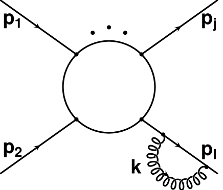
Figure 1: In an axial gauge, all collinear logarithms come from corrections to a particular external line (depending on the choice of the four vector $n^{\nu}$ satisfying $n^{\nu}A^{a}_{\nu}=0$) as illustrated in the figure. In a covariant gauge, the sum over all possible insertions is reduced to a sum over all $n$-external legs due to Ward identities. Overall, these corrections factorize with respect to the Born amplitude.

We can therefore adopt the strategy to extract the gauge invariant contribution from the external line corrections on the invariant matrix element at the subleading level. The results of the previous section are thus important in that they allow the use of the Altarelli-Parisi approach to calculate the subleading contribution to the evolution kernel of Eq. (4). We are here only concerned with virtual corrections and use the universality of the splitting functions to calculate the subleading terms. For this purpose we use the virtual quark and gluon contributions to the splitting functions $P^{V}_{qq}(z)$ and $P^{V}_{gg}(z)$ describing the probability to emit a soft and/or collinear virtual particle with energy fraction $z$ of the original external line four momentum. The infinite momentum frame corresponds to the Sudakov parametrization with lightlike vectors. In general, the splitting functions $P_{BA}$ describe the probability of finding a particle $B$ inside a particle $A$ with fraction $z$ of the longitudinal momentum of $A$ with probability ${\cal P}_{BA}$ to first order [12]:

$$d{\cal P}_{BA}(z)=\frac{\alpha_{s}}{2\pi}P_{BA}dt$$ (19)

where the variable $t=\log\frac{s}{\mu^{2}}$ for our purposes. It then follows [12] that

$$d{\cal P}_{BA}(z)=\frac{\alpha_{s}}{2\pi}\frac{z(1-z)}{2}\overline{\sum_{spins}}\frac{|V_{A\longrightarrow B+C}|^{2}}{{\mbox{\boldmath$k$}^{2}_{\perp}}}d\log{\mbox{\boldmath$k$}^{2}_{\perp}}$$ (20)

where $V_{A\longrightarrow B+C}$ denotes the elementary vertices and

$$P_{BA}(z)=\frac{z(1-z)}{2}\overline{\sum_{spins}}\frac{|V_{A\longrightarrow B+C}|^{2}}{{\mbox{\boldmath$k$}^{2}_{\perp}}}$$ (21)

The upper bound on the integral over $d{\mbox{\boldmath$k$}^{2}_{\perp}}$ in Eq. (20) is $s$ and it is thus directly related to $dt$. Regulating the virtual infrared divergences with the transverse momentum cutoff as described above, we find the virtual contributions to the splitting functions for external quark and gluon lines:

$$P^{V}_{qq}(z) = C_{F}\left(-2\log\frac{s}{\mu^{2}}+3\right)\delta(1-z)$$ (22)

$$P^{V}_{gg}(z) = C_{A}\left(-2\log\frac{s}{\mu^{2}}+\frac{4}{C_{A}}\beta^{\rm QCD}_{0}\right)\delta(1-z)$$ (23)

The functions can be calculated directly from loop corrections to the elementary processes [13, 14, 15] and the logarithmic term corresponds to the leading kernel of section 2.1. We introduce virtual distribution functions which include only the effects of loop computations. These fulfill the Altarelli-Parisi equations

$$\frac{\partial q(z,t)}{\partial t} = \frac{\alpha_{s}}{2\pi}\int^{1}_{z}\frac{dy}{y}q(z/y,t)P^{V}_{qq}(y)$$ (24)

$$\frac{\partial g(z,t)}{\partial t} = \frac{\alpha_{s}}{2\pi}\int^{1}_{z}\frac{dy}{y}g(z/y,t)P^{V}_{gg}(y)$$ (25)

The splitting functions are related by $P_{BA}=P^{R}_{BA}+P^{V}_{BA}$, where $R$ denotes the contribution from real gauge boson emission. $P_{BA}$ is free of logarithmic corrections and positive definite. The subleading term in Eq. (23) indicates that the only subleading corrections in the pure glue sector are related to a shift in the scale of the coupling. These corrections enter with a different sign compared to the conventional running coupling effects. The renormalizations with respect to the Born amplitude as well as the ones belonging to the next to leading terms at higher orders will be indicated below by writing $\alpha_{s}(\overline{\mu}^{2})\longrightarrow\alpha_{s}(s)$. For fermion lines there is an additional subleading correction from collinear terms which is not related to a change in the scale of the coupling.

Inserting the virtual probabilities of Eqs. (22) and (23) into the Eqs. (24) and (25) we find:

$$q(1,t) = q_{0}\exp\left[-\frac{\alpha_{s}(s)C_{F}}{2\pi}\left(\log^{2}\frac{s}{\mu^{2}}-3\log\frac{s}{\mu^{2}}\right)\right]$$ (26)

$$g(1,t) = g_{0}\exp\left[-\frac{\alpha_{s}(s)C_{A}}{2\pi}\left(\log^{2}\frac{s}{\mu^{2}}-\frac{4}{C_{A}}\beta^{\rm QCD}_{0}\log\frac{s}{\mu^{2}}\right)\right]$$ (27)

where $\beta^{\rm QCD}_{0}=\frac{11}{12}C_{A}-\frac{1}{3}T_{F}n_{f}$ with $C_{A}=3$ and $T_{F}=\frac{1}{2}$.

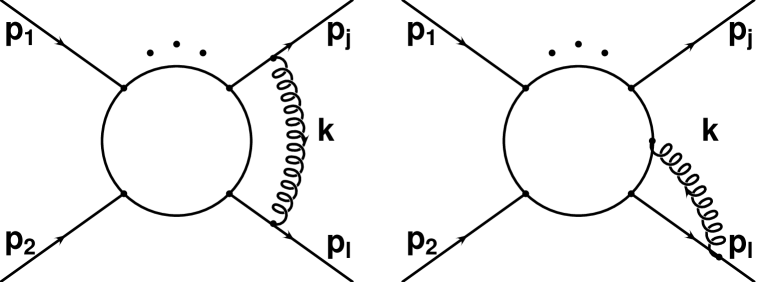
Figure 2: Feynman diagrams contributing to the infrared evolution equation (32) for a process with $n$ external legs. In a general covariant gauge the virtual gluon with the smallest value of ${\mbox{\boldmath$k$}}_{\perp}$ is attached to different external lines. The inner scattering amplitude is assumed to be on the mass shell.

These functions describe the total contribution for the emission of virtual particles (i.e. $z=1$), with all invariants large compared to the cutoff $\mu$, to the densities $q(z,t)$ and $g(z,t)$. The normalization is on the level of the cross section. For the invariant matrix element we thus find at the subleading level:

$${\cal M}(p_{1},...,p_{n},g_{s},\mu) = {\cal M}(p_{1},...,p_{n},g_{s}(s))\times$$ (28)

$$\exp\left(-\frac{1}{2}\sum^{n_{q}}_{j=1}W^{q}_{j}(s,\mu^{2})-\frac{1}{2}\sum^{n_{g}}_{l=1}W^{g}_{l}(s,\mu^{2})\right)$$

with $n_{q}+n_{g}=n$, and

$$W^{q}(s,\mu^{2}) = \frac{\alpha_{s}(s)C_{F}}{4\pi}\left(\log^{2}\frac{s}{\mu^{2}}-3\log\frac{s}{\mu^{2}}\right)$$ (29)

$$W^{g}(s,\mu^{2}) = \frac{\alpha_{s}(s)C_{A}}{4\pi}\left(\log^{2}\frac{s}{\mu^{2}}-\frac{4}{C_{A}}\beta^{\rm QCD}_{0}\log\frac{s}{\mu^{2}}\right)$$ (30)

Again we note that the running coupling notation in the Born-amplitude of Eq. (28) denotes the renormalization corrections of the Born amplitude and higher order corrections. The functions $W^{q}$, $W^{g}$ correspond to the probability of emitting a virtual soft and/or collinear gauge boson from the particle $q$, $g$ subject to the infrared cutoff $\mu$. Typical diagrams contributing to Eq. (28) in a covariant gauge are depicted in Fig. 2. In massless QCD there is no need for the label $W^{q}_{j}$ or $W^{g}_{l}$, however, we write it for later convenience. The universality of the splitting functions is crucial in obtaining the above result.

2.4 Renormalization group equation

The solution presented in Eq. (28) determines the evolution of the virtual scattering amplitude ${\cal M}(p_{1},...,p_{n},g_{s},\mu)$ for large energies at fixed angles and subject to the infrared regulator $\mu$. In the massless case there is a one to one correspondence between the high energy limit and the infrared limit as only the ratio $s/\mu^{2}$ enters as a dimensionless variable [17, 18]. Thus, we can generalize the Altarelli-Parisi equations (24) and (25) to the invariant matrix element in the language of the renormalization group. For this purpose, we define the infrared singular (logarithmic) anomalous dimensions

$$\Gamma_{q}(t)\equiv\frac{C_{F}\alpha_{s}}{4\pi}t\;\;;\;\;\Gamma_{g}(t)\equiv\frac{C_{A}\alpha_{s}}{4\pi}t$$ (31)

Infrared divergent anomalous dimensions have been derived in the context of renormalization properties of gauge invariant Wilson loop functionals [19]. In this context they are related to undifferentiable cusps of the path integration and the cusp angle $~{}p_{j}p_{l}/\mu^{2}$ gives rise to the logarithmic nature of the anomalous dimension. In case we use off-shell amplitudes, one also has contributions from end points of the integration [19]. The leading terms in the equation below have also been discussed in Refs. [20], [21] and [22] in the context of QCD. With these notations we find that Eq. (28) satisfies

$$\left(\frac{\partial}{\partial t}+\beta^{\rm QCD}\frac{\partial}{\partial g_{s}}+n_{g}\left(\Gamma_{g}(t)-\frac{1}{2}\frac{\alpha_{s}}{\pi}\beta^{\rm QCD}_{0}\right)+n_{q}\left(\Gamma_{q}(t)+\frac{1}{2}\gamma_{q\overline{q}}\right)\right)$$

$$\times{\cal M}(p_{1},...,p_{n},g_{s},\mu)=0$$ (32)

to the order we are working here and where ${\cal M}(p_{1},...,p_{n},g_{s},\mu)$ is taken on the mass-shell. The difference in the sign of the derivative term compared to Eq. (4) is due to the fact that instead of differentiating with respect to $\log\mu^{2}$ we use $\log s/\mu^{2}$. The quark-antiquark operator anomalous dimension $\gamma_{q\overline{q}}=-C_{F}\frac{3}{4}\frac{\alpha}{\pi}$ enters even for massless theories as the quark antiquark operator leads to scaling violations through loop effects since the quark masslessness is not protected by gauge invariance and a dimensionful infrared cutoff needs to be introduced. Thus, although the Lagrangian contains no $mq\overline{q}$ term, quantum corrections lead to the anomalous scaling violations in the form of $\gamma_{q\overline{q}}$. The factor $\frac{1}{2}$ occurs since we write Eq. (32) in terms of each external line separately. For the gluon, the scaling violation due to the infrared cutoff are manifest in terms of an anomalous dimension proportional to the $\beta$-function since the gluon mass is protected by gauge invariance from loop corrections. Thus, in the bosonic sector the subleading terms correspond effectively to a scale change of the coupling. Fig. 3 illustrates the corrections to the external quark-antiquark lines from loop effects.

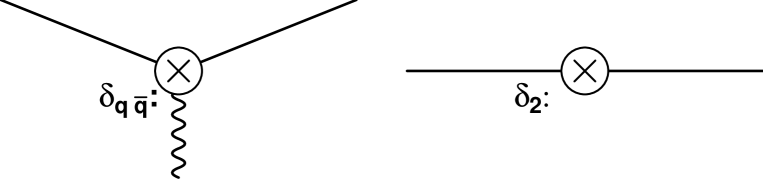
Figure 3: The two counterterms contributing to the quark anomalous dimension $\gamma_{q\overline{q}}=\frac{\partial}{\partial\log\overline{\mu}^{2}}\left(-\delta_{q\overline{q}}+\delta_{2}\right)$. Here $\overline{\mu}$ denotes the $\overline{\rm MS}$ dimensional regularization mass parameter. Due to divergences in loop corrections there are scaling violations also in the massless theory.

Except for the infrared singular anomalous dimension (Eq. (31)), all other terms in Eq. (32) are the standard contributions to the renormalization group equation for S-matrix elements [23]. In QCD, observables with infrared singular anomalous dimensions, regulated with a fictitious gluon mass, are ill defined due to the masslessness of gluons. In the electroweak theory, however, we can legitimately investigate only virtual corrections since the gauge bosons will require a mass. Eq. (32) will thus be very useful in the following sections.

3 Logarithmic corrections in broken gauge theories

In the following we will apply the results obtained in the previous sections to the case of spontaneously broken gauge theories. It will be necessary, at least at the subleading level, to distinguish between transverse and longitudinal degrees of freedom. The physical motivation in this approach is that for very large energies, $s\gg M_{W}^{2}\equiv M^{2}$, the electroweak theory is in the unbroken phase, with an exact $SU(2)\times U(1)$ gauge symmetry. We will calculate the corrections to this theory and use the high energy solution as a matching condition for the regime for values of $\mu<M$.

We begin by considering some simple kinematic arguments for massive vector bosons. A vector boson at rest has momentum $k^{\nu}=(M,0,0,0)$ and a polarization vector that is a linear combination of the three orthogonal unit vectors

$$e_{1}\equiv(0,1,0,0)\;\;\;,\;\;\;e_{1}\equiv(0,0,1,0)\;\;\;,\;\;\;e_{3}\equiv(0,0,0,1)\;\;\;.$$ (33)

After boosting this particle along the $3$-axis, its momentum will be $k^{\nu}=(E_{k},0,0,k)$. The three possible polarization vectors are now still satisfying:

$$k_{\nu}e^{\nu}_{j}=0\;\;\;,\;\;\;e_{j}^{2}=-1\;\;\;.$$ (34)

Two of these vectors correspond to $e_{1}$ and $e_{2}$ and describe the transverse polarizations. The third vector satisfying (34) is the longitudinal polarization vector

$$e_{L}^{\nu}(k)=(k/M,0,0,E_{k}/M)$$ (35)

i.e. $e_{L}^{\nu}(k)=k^{\nu}/M+{\cal O}(M/E_{k})$ for large energies. These considerations illustrate that the transversely polarized degrees of freedom at high energies are related to the massless theory, while the longitudinal degrees of freedom need to be considered separately.

Another manifestation of the different high energy nature of the two polarization states is contained in the Goldstone boson equivalence theorem. It states that the unphysical Goldstone boson that is “eaten up” by a massive gauge boson still controls its high energy asymptotics. A more precise formulation is given below in section 3.2.

Thus we can legitimately use the results obtained in the massless non-Abelian theory if we restrict ourselves to the transverse degrees of freedom at high energies. We will, however, show that to DL accuracy the results of Ref. [1] can be used in connection with the Goldstone boson equivalence theorem.

Another difference to the situation in an unbroken non-Abelian theory is the mixing of the physical fields with the fields in the unbroken phase. These complications are especially relevant for the $Z$-boson and the photon.

3.1 Results for transverse degrees of freedom

The results we obtain in this section are generally valid for spontaneously broken gauge theories, however, for definiteness we discuss only the electroweak Standard Model. The physical gauge bosons are thus a massless photon (described by the field $A_{\nu}$) and massive $W^{\pm}$ and $Z$ bosons (described correspondingly by fields $W_{\nu}^{\pm}$ and $Z_{\nu}$).:

$$W^{\pm}_{\nu} = \frac{1}{\sqrt{2}}\left(W^{1}_{\nu}\pm iW^{2}_{\nu}\right)$$ (36)

$$Z_{\nu} = \cos\theta_{\rm w}W^{3}_{\nu}+\sin\theta_{\rm w}B_{\nu}$$ (37)

$$A_{\nu} = -\sin\theta_{\rm w}W^{3}_{\nu}+\cos\theta_{\rm w}B_{\nu}$$ (38)

Thus, amplitudes containing physical fields will correspond to a linear combination of the massless fields in the unbroken phase. The situation is illustrated schematically for a single gauge boson external leg in Fig. 4. In case of the $W^{\pm}$ bosons, the corrections factorize with respect to the physical amplitude.

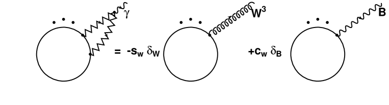
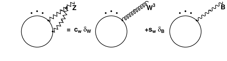
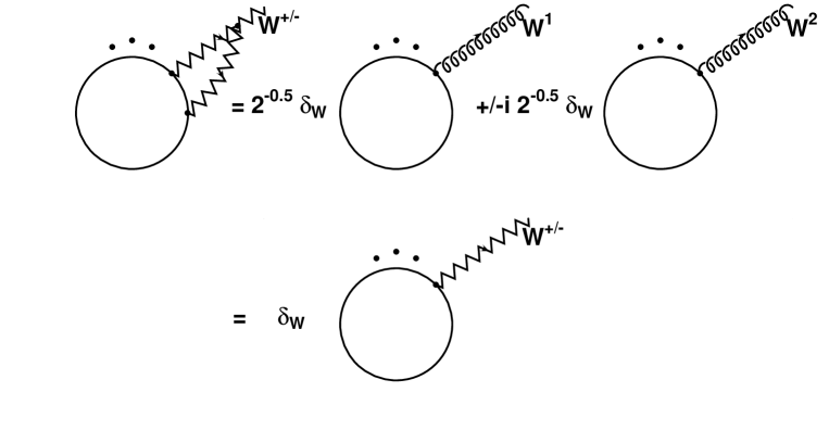
Figure 4: The schematic corrections to external gauge boson emissions in terms of the fields in the unbroken phase of the electroweak theory. There are no mixing terms between the $W^{3}_{\nu}$ and $B_{\nu}$ fields for massless fermions. We denote $\cos\theta_{\rm w}$ by $c_{\rm w}$ and $\sin\theta_{\rm w}$ by $s_{\rm w}$. For $W^{\pm}$ final states, the corrections factorize with respect to the physical amplitude. In general, one has to sum over all fields of the unbroken theory with each amplitude being multiplied by the respective mixing coefficient.

To logarithmic accuracy, all masses can be set equal:

$$M_{Z}\sim M_{W}\sim M_{\rm Higgs}\sim M$$

and the energy considered to be much larger, $\sqrt{s}\gg M$. The physical fields are given in terms of the unbroken fields according to Eqs. (36), (37) and (38). The left and right handed fermions are correspondingly doublets ($T=1/2$) and singlets ($T=0$) of the $SU$(2) weak isospin group and have hypercharge $Y$ related to the electric charge $Q$, measured in units of the proton charge, by the Gell-Mann-Nishijima formula $Q=T^{3}+Y/2$.

The value for the infrared cutoff $\mu$ can be chosen in two different regimes: 1) $\sqrt{s}\gg\mu\gg M$ and 2) $\mu\ll M$. The second case is universal in the sense that it does not depend on the details of the electroweak theory and will be discussed below. In the first region we can neglect spontaneous symmetry breaking effects (in particular gauge boson masses) and consider the theory with fields $B_{\nu}$ and $W_{\nu}^{a}$. One could of course also calculate everything in terms of the physical fields, however, we emphasize again that in this case we need to consider the photon also in region 1). The omission of the photon would lead to the violation of gauge invariance since the photon contains a mixture of the $B_{\nu}$ and $W_{\nu}^{3}$ fields.

In region 1), the renormalization group equation (or generalized infrared evolution equation) (32) in the case of all $m_{i}<M$ reads

$$\left(\frac{\partial}{\partial t}+\beta\frac{\partial}{\partial g}+\beta^{\prime}\frac{\partial}{\partial g^{\prime}}+\sum_{i=1}^{n_{g}}\Gamma^{i}_{g}(t)-n_{\rm W}\frac{1}{2}\frac{\alpha}{\pi}\beta_{0}-n_{\rm B}\frac{1}{2}\frac{\alpha^{\prime}}{\pi}\beta^{\prime}_{0}+\sum_{k=1}^{n_{f}}\left(\Gamma^{k}_{f}(t)+\frac{1}{2}\gamma^{k}_{q\overline{q}}\right)\right)$$

$$\times{\cal M}^{\perp}(p_{1},...,p_{n},g,g^{\prime},\mu)=0$$ (39)

where the index $\perp$ indicates that we consider only $n_{g}$ transversely polarized external gauge bosons and $n_{\rm W}+n_{\rm B}=n_{g}$. The two $\beta$-functions are given by:

$$\beta(g(\overline{\mu}^{2})) = \frac{\partial g(\overline{\mu}^{2})}{\partial\log\overline{\mu}^{2}}\approx-\beta_{0}\frac{g^{3}(\overline{\mu}^{2})}{8\pi^{2}}$$ (40)

$$\beta^{\prime}(g^{\prime}(\overline{\mu}^{2})) = \frac{\partial g^{\prime}(\overline{\mu}^{2})}{\partial\log\overline{\mu}^{2}}\approx-\beta^{\prime}_{0}\frac{{g^{\prime}}^{3}(\overline{\mu}^{2})}{8\pi^{2}}$$ (41)

with the one-loop terms given by:

$$\beta_{0}=\frac{11}{12}C_{A}-\frac{1}{3}n_{gen}-\frac{1}{24}n_{h}\;\;\;,\;\;\;\beta^{\prime}_{0}=-\frac{5}{9}n_{gen}-\frac{1}{24}n_{h}$$ (42)

where $n_{gen}$ denotes the number of fermion generations [24, 25] and $n_{h}$ the number of Higgs doublets. The infrared singular anomalous dimensions read

$$\Gamma^{i}_{f,g}(t)=\left(\frac{\alpha}{4\pi}T_{i}(T_{i}+1)+\frac{\alpha^{\prime}}{4\pi}\left(\frac{Y_{i}}{2}\right)^{2}\right)t$$ (43)

where $T_{i}$ and $Y_{i}$ are the total weak isospin and hypercharge respectively of the particle emitting the soft and collinear gauge boson. Analogously,

$$\gamma^{i}_{q\overline{q}}=-3\left(\frac{\alpha}{4\pi}T_{i}(T_{i}+1)+\frac{\alpha^{\prime}}{4\pi}\left(\frac{Y_{i}}{2}\right)^{2}\right)$$ (44)

The initial condition for Eq. (39) is given by the requirement that for the infrared cutoff $\mu^{2}=s$ we obtain the Born amplitude. The solution of (39) is thus given by

$${\cal M}^{\perp}(p_{1},...,p_{n},g,g^{\prime},\mu)={\cal M}^{\perp}_{\rm Born}(p_{1},...,p_{n},g(s),g^{\prime}(s))$$

$$\times\exp\left\{-\frac{1}{2}\sum^{n_{g}}_{i=1}\left(\frac{\alpha(s)}{4\pi}T_{i}(T_{i}+1)+\frac{\alpha^{\prime}(s)}{4\pi}\left(\frac{Y_{i}}{2}\right)^{2}\right)\log^{2}\frac{s}{\mu^{2}}\right.$$

$$\;\;\;\;\;\;\;\;\;\;\;\;+\left(n_{\rm W}\frac{\alpha(s)}{2\pi}\beta_{0}+n_{\rm B}\frac{\alpha^{\prime}(s)}{2\pi}\beta^{\prime}_{0}\right)\log\frac{s}{\mu^{2}}$$

$$-\frac{1}{2}\left.\sum^{n_{f}}_{k=1}\left(\frac{\alpha(s)}{4\pi}T_{k}(T_{k}+1)+\frac{\alpha^{\prime}(s)}{4\pi}\left(\frac{Y_{k}}{2}\right)^{2}\right)\left[\log^{2}\frac{s}{\mu^{2}}-3\log\frac{s}{\mu^{2}}\right]\right\}$$ (45)

where $n_{\rm W}$ and $n_{\rm B}$ denote the number of external $W$ and $B$ fields respectively. The $SU(2)\times U(1)$ group factors in the exponential can be written in terms of the parameters of the broken theory as follows:

$$g^{2}T_{i}(T_{i}+1)+{g^{\prime}}^{2}\left(\frac{Y_{i}}{2}\right)^{2}=e_{i}^{2}+g^{2}\left(T_{i}(T_{i}+1)-(T_{i}^{3})^{2}\right)+\frac{g^{2}}{\cos^{2}\theta_{w}}\left(T_{i}^{3}-\sin^{2}\theta_{w}Q_{i}\right)^{2},$$

where the three terms on the r.h.s. correspond to the contributions of the soft photon (interacting with the electric charge $e_{i}=Q_{i}g\sin\theta_{w}$), the $W^{\pm}$ and the $Z$ bosons, respectively. Although we may rewrite solution (45) in terms of the parameters of the broken theory in the form of a product of three exponents corresponding to the exchanges of photons, $W^{\pm}$ and $Z$ bosons, it would be wrong to identify the contributions of the diagrams without virtual photons with this expression for the particular case $e_{i}^{2}=0$. This becomes evident when we note that if we were to omit photon lines then the result would depend on the choice of gauge, and therefore be unphysical. Only for $\theta_{w}=0$, where the photon coincides with the $B$ gauge boson, would the identification of the $e_{i}^{2}$ term with the contribution of the diagrams with photons be correct.

We now need to discuss the solution in the general case. In region 1) we calculated the scattering amplitude for the theory in the unbroken phase in the massless limit. Choosing the cutoff $\mu$ in region 2), $\mu\ll M$, we have to only consider the photon contribution. In this region we cannot necessarily neglect all mass terms, so we need to discuss the subleading terms for QED with mass effects. If $m_{i}\ll\mu$, the results from the massless QCD discussion of section 2.3 can be used directly by using the Abelian limit $C_{F}=1$. In case $\mu\ll m_{i}$ we must use the well known next to leading order QED results, e.g. [26], and the virtual probabilities take the following form for fermions:

$$w^{f}_{i}(s,\mu^{2})=\left\{\begin{array}[]{lc}\frac{e_{i}^{2}}{(4\pi)^{2}}\left(\log^{2}\frac{s}{\mu^{2}}-3\log\frac{s}{\mu^{2}}\right)&,\;\;\;m_{i}\ll\mu\\ \frac{e_{i}^{2}}{(4\pi)^{2}}\left[\left(\log\frac{s}{m_{i}^{2}}-1\right)2\log\frac{m_{i}^{2}}{\mu^{2}}\right.\\ \left.\;\;\;\;\;\;\;\;\;\;+\log^{2}\frac{s}{m_{i}^{2}}-3\log\frac{s}{m_{i}^{2}}\right]&,\;\;\;\mu\ll m_{i}\end{array}\right.$$ (46)

Note, that in the last equation the full subleading collinear logarithmic term [10] is used in distinction to Ref. [26]. In the explicit two loop calculation presented in Ref. [27] it can be seen that the full collinear term also exponentiates at the subleading level in massive QED. For $W^{\pm}$ bosons we have analogously:

$$w^{\rm w}_{i}(s,\mu^{2})=\frac{e_{i}^{2}}{(4\pi)^{2}}\left[\left(\log\frac{s}{M^{2}}-1\right)2\log\frac{M^{2}}{\mu^{2}}+\log^{2}\frac{s}{M^{2}}\right]$$ (47)

In addition we have collinear terms for external on-shell photon lines from fermions with mass $m_{j}$ and electromagnetic charge $e_{j}$ up to scale $M$:

$$w_{i}^{\gamma}(M^{2},\mu^{2})=\left\{\begin{array}[]{lc}\frac{n_{f}}{3}\frac{e_{j}^{2}}{4\pi^{2}}N^{j}_{C}\log\frac{M^{2}}{\mu^{2}}&,\;\;\;m_{j}\ll\mu\\ \frac{1}{3}\sum_{j=1}^{n_{f}}\frac{e_{j}^{2}}{4\pi^{2}}N^{j}_{C}\log\frac{M^{2}}{m_{j}^{2}}&,\;\;\;\mu\ll m_{j}\end{array}\right.$$ (48)

Note that automatically, $w_{i}^{\gamma}(M^{2},M^{2})=0$. At one loop order, this contribution cancels against terms from the renormalization of the QED coupling up to scale $M$. For external $Z$-bosons, however, there are no such collinear terms since the mass is large compared to the $m_{i}$. Thus, the corresponding RG-logarithms up to scale $M$ remain uncanceled.

The appropriate initial condition is given by Eq. (45) evaluated at the matching point $\mu=M$. Thus we find for the general solution in region 2):

$${\cal M}^{\perp}(p_{1},...,p_{n},g,g^{\prime},\mu)={\cal M}^{\perp}_{\rm Born}(p_{1},...,p_{n},g(s),g^{\prime}(s))$$

$$\times\exp\left\{-\frac{1}{2}\sum^{n_{g}}_{i=1}\left(\frac{\alpha(s)}{4\pi}T_{i}(T_{i}+1)+\frac{\alpha^{\prime}(s)}{4\pi}\left(\frac{Y_{i}}{2}\right)^{2}\right)\log^{2}\frac{s}{M^{2}}\right.$$

$$\;\;\;\;\;\;\;\;\;\;\;\;+\left(n_{\rm W}\frac{\alpha(s)}{2\pi}\beta_{0}+n_{\rm B}\frac{\alpha^{\prime}(s)}{2\pi}\beta^{\prime}_{0}\right)\log\frac{s}{M^{2}}$$

$$-\frac{1}{2}\left.\sum^{n_{f}}_{k=1}\left(\frac{\alpha(s)}{4\pi}T_{k}(T_{k}+1)+\frac{\alpha^{\prime}(s)}{4\pi}\left(\frac{Y_{k}}{2}\right)^{2}\right)\left[\log^{2}\frac{s}{M^{2}}-3\log\frac{s}{M^{2}}\right]\right\}$$

$$\times\exp\left[-\frac{1}{2}\sum_{i=1}^{n_{f}}\left(w^{f}_{i}(s,\mu^{2})-w^{f}_{i}(s,M^{2})\right)-\frac{1}{2}\sum_{i=1}^{n_{w}}\left(w^{\rm w}_{i}(s,\mu^{2})-w^{\rm w}_{i}(s,M^{2})\right)\right.$$

$$\;\;\;\;\;\;\;\;\;\;\;\left.-\frac{1}{2}\sum_{i=1}^{n_{\gamma}}w_{i}^{\gamma}(M^{2},\mu^{2})\right]$$

$$={\cal M}^{\perp}_{\rm Born}(p_{1},...,p_{n},g(s),g^{\prime}(s))$$

$$\times\exp\left\{-\frac{1}{2}\sum^{n_{g}}_{i=1}\left(\frac{\alpha(s)}{4\pi}T_{i}(T_{i}+1)+\frac{\alpha^{\prime}(s)}{4\pi}\left(\frac{Y_{i}}{2}\right)^{2}\right)\log^{2}\frac{s}{M^{2}}\right.$$

$$\;\;\;\;\;\;\;\;\;\;\;\;+\left(n_{\rm W}\frac{\alpha(s)}{2\pi}\beta_{0}+n_{\rm B}\frac{\alpha^{\prime}(s)}{2\pi}\beta^{\prime}_{0}\right)\log\frac{s}{M^{2}}$$

$$-\frac{1}{2}\left.\sum^{n_{f}}_{k=1}\left(\frac{\alpha(s)}{4\pi}T_{k}(T_{k}+1)+\frac{\alpha^{\prime}(s)}{4\pi}\left(\frac{Y_{k}}{2}\right)^{2}\right)\left[\log^{2}\frac{s}{M^{2}}-3\log\frac{s}{M^{2}}\right]\right\}$$

$$\times\exp\left[-\frac{1}{2}\sum_{i=1}^{n}\!\left(\frac{e_{i}^{2}(s)}{(4\pi)^{2}}\!\left(2\log\frac{s}{m_{i}\,M}\log\frac{M^{2}}{m_{i}^{2}}+2\log\frac{s}{m_{i}^{2}}\log\frac{m_{i}^{2}}{\mu^{2}}+3\log\frac{m_{i}^{2}}{M^{2}}\right.\right.\right.$$

$$\left.\left.\left.-2\log\frac{m_{i}^{2}}{\mu^{2}}\right)\right)-\frac{1}{2}\sum_{i=1}^{n_{\gamma}}\frac{1}{3}\frac{e_{i}^{2}}{4\pi^{2}}N^{i}_{C}\log\frac{M^{2}}{m_{i}^{2}}\right]$$ (49)

The last equality holds for $\mu\ll m_{i}\ll M$ and we have absorbed all $\beta$-function terms not related to external lines into redefinitions of the scales of the couplings. It is important to note again that, unlike the situation in QCD, in the electroweak theory we have in general different mass scales determining the running of the couplings of the physical on-shell renormalization scheme quantities. We have written the above result in such a way that it holds for arbitrary chiral fermions and transversely polarized gauge bosons. In order to include physical external photon states in the on-shell scheme, the renormalization condition is given by the requirement that the physical photon does not mix with the Z-boson. This leads to the condition that the Weinberg rotations in Fig. 4 at one loop receive no RG-corrections. Thus, above the scale $M$ the subleading collinear and RG-corrections cancel for physical photon and Z-boson states. For physical observables, soft real photon emission must be taken into account in an inclusive (or semi inclusive) way and the parameter $\mu^{2}$ in (49) will be replaced by parameters depending on the experimental requirements. This will be briefly discussed in the following section.

3.1.1 Semi inclusive cross sections

In order to make predictions for observable cross sections, the unphysical infrared cutoff $\mu^{2}$ has to be replaced with a cutoff $\mu^{2}_{exp}$, related to the lower bound of $\mbox{\boldmath$k$}_{\perp}^{2}$ of the other virtual particles of those gauge bosons emitted in the process which are not included in the cross section. We assume that $\mu^{2}_{exp}<M^{2}$, so that the non-Abelian component of the photon is not essential. The case $\mu^{2}_{exp}>M^{2}$ is much more complicated and is discussed in Ref. [1] through two loops at the DL level.

We again only discuss transversely polarized external gauge boson in the Born process and can write the expression for the semi-inclusive cross section:

$$d\sigma^{\perp}(p_{1},\ldots,p_{n},g,g^{\prime},\mu_{exp}) = d\sigma^{\perp}_{\rm elastic}(p_{1},\ldots,p_{n},g(s),g^{\prime}(s),\mu)$$ (50)

$$\times\exp(w_{\exp}^{\gamma}(s,m_{i},\mu,\mu_{exp}))$$

In the soft photon approximation we have:

$$w_{\exp}^{\gamma}(s,m_{i},\mu,\mu_{exp})\!\! = \!\!\!\left\{\begin{array}[]{lc}\frac{e_{i}^{2}}{(4\pi)^{2}}\sum_{i=1}^{n}\left[-\log^{2}\frac{s}{\mu^{2}_{exp}}+\log^{2}\frac{s}{\mu^{2}}-3\log\frac{s}{\mu^{2}}\right]&,m_{i}\ll\mu\\ \frac{e_{i}^{2}}{(4\pi)^{2}}\sum_{i=1}^{n}\left[\left(\log\frac{s}{m_{i}^{2}}-1\right)2\log\frac{m_{i}^{2}}{\mu^{2}}+\log^{2}\frac{s}{m_{i}^{2}}\right.\\ \left.-2\log\frac{s}{\mu^{2}_{exp}}\left(\log\frac{s}{m_{i}^{2}}-1\right)\right]&,\mu\ll m_{i}\end{array}\right.$$ (54)

where the upper case applies only to fermions since for $W^{\pm}$ we have $\mu<M$ in region 2). Since the upper bound on ${\mbox{\boldmath$k$}_{\perp}^{2}}$ of the photons which are allowed to be radiated is less than $M^{2}$, we must use the cut-off $\mu^{2}<M^{2}$ and, consequently, (49) for the matrix element of the non-radiative process. Therefore, we obtain

$$d\sigma^{\perp}(p_{1},\ldots,p_{n},g,g^{\prime},\mu_{exp})=d\sigma_{\rm Born}^{\perp}(p_{1},\ldots,p_{n},g(s),g^{\prime}(s))$$

$$\times\exp\left\{-\sum^{n_{g}}_{i=1}\left(\frac{\alpha(s)}{4\pi}T_{i}(T_{i}+1)+\frac{\alpha^{\prime}(s)}{4\pi}\left(\frac{Y_{i}}{2}\right)^{2}\right)\log^{2}\frac{s}{M^{2}}\right.$$

$$\;\;\;\;\;\;\;\;\;\;\;\;+\left(n_{\rm W}\frac{\alpha(s)}{\pi}\beta_{0}+n_{\rm B}\frac{\alpha^{\prime}(s)}{\pi}\beta^{\prime}_{0}\right)\log\frac{s}{M^{2}}$$

$$\left.-\sum^{n_{f}}_{k=1}\left(\frac{\alpha(s)}{4\pi}T_{k}(T_{k}+1)+\frac{\alpha^{\prime}(s)}{4\pi}\left(\frac{Y_{k}}{2}\right)^{2}\right)\left[\log^{2}\frac{s}{M^{2}}-3\log\frac{s}{M^{2}}\right]\right\}$$

$$\times\exp\left[-\sum_{i=1}^{n_{f}}\left(w^{f}_{i}(s,\mu^{2})-w^{f}_{i}(s,M^{2})\right)-\sum_{i=1}^{n_{w}}\left(w^{\rm w}_{i}(s,\mu^{2})-w^{\rm w}_{i}(s,M^{2})\right)\right.$$

$$\;\;\;\;\;\;\;\;\;\;\;\left.-\sum_{i=1}^{n_{\gamma}}w_{i}^{\gamma}(M^{2},m_{j}^{2})\right]$$

$$\times\exp\left(\frac{e_{i}^{2}}{(4\pi)^{2}}\sum_{i=1}^{n}\left[\left(\log\frac{s}{m_{i}^{2}}-1\right)2\log\frac{m_{i}^{2}}{\mu^{2}}-2\log\frac{s}{\mu^{2}_{exp}}\left(\log\frac{s}{m_{i}^{2}}-1\right)\right.\right.$$

$$\left.\left.+\log^{2}\frac{s}{m_{i}^{2}}\right]\right)$$ (56)

where we use $\mu\ll m_{i}$. The $\mu$ dependence in this expression cancels and the semi-inclusive cross section depends only on the parameters of the experimental requirements.

Eq. (56) contains all leading double and single logarithms to cross sections containing arbitrary numbers of external fermions and transversely polarized gauge bosons. We have only assumed that all masses are not larger than the electroweak scale $M$ and impose a cut on the the allowed values of emitted real gauge bosons ${\mbox{\boldmath$k$}_{\perp}^{2}}\leq\mu^{2}_{exp}<M^{2}$, i.e. up to the weak scale we only need to consider real QED effects.

3.2 Longitudinal degrees of freedom

In this section we discuss if results obtained from the massless unbroken phase of the $SU(2)\times U(1)$ theory, where due to gauge invariance we have only transverse physical degrees of freedom, can be extended to the full theory including longitudinal vector bosons. This point of discussion is necessary and important since the longitudinal degrees of freedom don’t decouple at high energies and could give crucial clues to potentially strong dynamical effects for large Higgs masses $m_{H}\sim 1TeV$ [24].

The connection between the strategy pursued for the transverse degrees of freedom and the corrections to longitudinally polarized vector bosons at high energies is provided by the Goldstone boson equivalence theorem [28]. It states that at tree level for S-matrix elements for longitudinal bosons at the high energy limit $M^{2}/s\longrightarrow 0$ can be expressed through matrix elements involving their associated would be Goldstone bosons. We write schematically in case of a single gauge boson:

$${\cal M}(W^{\pm}_{L},\psi_{{\rm phys}}) = {\cal M}(\phi^{\pm},\psi_{{\rm phys}})+{\cal O}\left(\frac{M_{\rm w}}{\sqrt{s}}\right)$$ (57)

$${\cal M}(Z_{L},\psi_{{\rm phys}}) = {\cal M}(\phi,\psi_{{\rm phys}})+{\cal O}\left(\frac{M_{\rm z}}{\sqrt{s}}\right)$$ (58)

The problem with this statement of the equivalence theorem is that it holds only at tree level [29, 30]. For calculations at higher orders, additional terms enter which change Eqs. (57) and (58).

Because of the gauge invariance of the physical theory and the associated BRST invariance, a modified version of Eqs. (57) and (58) can be derived [29] which reads

$$k^{\nu}{\cal M}(W^{\pm}_{\nu}(k),\psi_{{\rm phys}}) = C_{\rm w}M_{\rm w}{\cal M}(\phi^{\pm}(k),\psi_{{\rm phys}})+{\cal O}\left(\frac{M_{\rm w}}{\sqrt{s}}\right)$$ (59)

$$k^{\nu}{\cal M}(Z_{\nu}(k),\psi_{{\rm phys}}) = C_{\rm z}M_{\rm z}{\cal M}(\phi(k),\psi_{{\rm phys}})+{\cal O}\left(\frac{M_{\rm z}}{\sqrt{s}}\right)$$ (60)

where the multiplicative factors $C_{\rm w}$ and $C_{\rm z}$ depend only on wave function renormalization constants and mass counterterms. Thus, using the form of the longitudinal polarization vector of Eq. (35) we can write

$${\cal M}(W^{\pm}_{L}(k),\psi_{{\rm phys}}) = C_{\rm w}{\cal M}(\phi^{\pm}(k),\psi_{{\rm phys}})+{\cal O}\left(\frac{M_{\rm w}}{\sqrt{s}}\right)$$ (61)

$${\cal M}(Z_{L}(k),\psi_{{\rm phys}}) = C_{\rm z}{\cal M}(\phi(k),\psi_{{\rm phys}})+{\cal O}\left(\frac{M_{\rm z}}{\sqrt{s}}\right)$$ (62)

Thus we see that in principle, there are logarithmic loop corrections to the tree level equivalence theorem. In addition, for longitudinal gauge bosons we also have logarithmic corrections with Yukawa terms [6]. On the one hand, this means that the method of section 3.1 should be used with caution to obtain the relevant subleading terms. Thus we should consider these corrections separately. On the other, since the corrections are at most logarithmic, it means that the results of Ref. [1] can be extended to the longitudinal sector as well. Thus we find for $\mu_{exp}<M$:

$$d\sigma^{\parallel}(p_{1},\ldots,p_{n},g,g^{\prime},\mu_{exp})=d\sigma_{\rm Born}^{\phi}(p_{1},\ldots,p_{n},g,g^{\prime})$$

$$\times\exp\left\{-\sum^{n}_{i=1}\left(\frac{\alpha}{4\pi}T_{i}(T_{i}+1)+\frac{\alpha^{\prime}}{4\pi}\left(\frac{Y_{i}}{2}\right)^{2}\right)\log^{2}\frac{s}{M^{2}}\right\}$$

$$\times\exp\left[-\sum_{i=1}^{n}\left(w^{{\rm DL}}_{i}(s,\mu^{2})-w^{{\rm DL}}_{i}(s,M^{2})\right)+w^{{\rm DL}}_{exp}\right]$$ (63)

where the index $\parallel$ indicates the cross section for longitudinally polarized gauge bosons, while the field $\phi$ indicates that the appropriate fields and quantum numbers on the r.h.s. in Eq. (63) are those of the associated would be Goldstone bosons.

Thus, we have shown that all DL corrections can be summed to all orders by employing the evolution equation approach of Ref. [1] in connection with the Goldstone boson equivalence theorem.

4 Comparison with explicit results

In this section we compare our results obtained in the previous sections with known results in special cases and one loop calculations. In Ref. [32], QCD-results for the Sudakov form factor were generalized to the high energy electroweak theory. Since the general strategy pursued is the same as in Ref. [1], we of course agree with their result for leading and subleading electroweak corrections to $e^{+}e^{-}\longrightarrow f\overline{f}$ to all orders.

Figure 5: The pictorial Goldstone boson equivalence theorem for $W$-pair production in $e^{+}e^{-}$ collisions. The correct DL-asymptotics for longitudinally polarized bosons are obtained by using the quantum numbers of the charged would be Goldstone scalars at high energies.

A very important check is provided by the explicit one-loop corrections of Ref. [6] for high energy on-shell $W$-pair production in the soft photon approximation. In the following, the lower index on the cross section indicates the helicity of the electron, where $e^{-}_{-}$ denotes the left handed electron. We summarize the relevant results for $e^{+}_{+}e^{-}_{-}\longrightarrow W^{+}_{\perp}W^{-}_{\perp}$, $e^{+}_{+}e^{-}_{-}\longrightarrow W^{+}_{\parallel}W^{-}_{\parallel}$ and $e^{+}_{-}e^{-}_{+}\longrightarrow W^{+}_{\parallel}W^{-}_{\parallel}$ for convenience as follows:

$$\left(\frac{d\sigma}{d\Omega}\right)_{-,\,\perp}\!\! \approx \!\!\left(\frac{d\sigma}{d\Omega}\right)^{\rm\!\!Born}_{-,\,\perp}\!\!\left\{1+\frac{e^{2}}{8\pi^{2}}\left[-\frac{1+2c_{\rm w}^{2}+8c_{\rm w}^{4}}{4c_{\rm w}^{2}s_{\rm w}^{2}}\log^{2}\frac{s}{M^{2}}+3\frac{1-2c_{\rm w}^{2}+4c_{\rm w}^{4}}{4c_{\rm w}^{2}s_{\rm w}^{2}}\log\frac{s}{M^{2}}\right.\right.$$ (64)

$$\left.\left.+3\log\frac{s}{m_{e}^{2}}+2\log\frac{4\Delta E^{2}}{s}\left(\log\frac{s}{m_{e}^{2}}+\log\frac{s}{M^{2}}-2\right)\right.\right.$$

$$\left.\left.-\frac{4}{3}\sum_{j=1}^{n_{f}}Q_{j}^{2}N^{j}_{C}\log\frac{m_{j}^{2}}{M^{2}}\right]\right\}$$

$$\left(\frac{d\sigma}{d\Omega}\right)_{-,\,\parallel} \approx \left(\frac{d\sigma}{d\Omega}\right)^{\rm Born}_{-,\,\parallel}\left\{1+\frac{e^{2}}{8\pi^{2}}\left[-\frac{1-2c_{\rm w}^{2}+4c_{\rm w}^{4}}{2c_{\rm w}^{2}s_{\rm w}^{2}}\log^{2}\frac{s}{M^{2}}\right.\right.$$ (65)

$$\left.\left.+2\log\frac{4\Delta E^{2}}{s}\left(\log\frac{s}{m_{e}^{2}}+\log\frac{s}{M^{2}}\right)\right]\right\}$$

$$\left(\frac{d\sigma}{d\Omega}\right)_{+,\,\parallel} \approx \left(\frac{d\sigma}{d\Omega}\right)^{\rm Born}_{+,\,\parallel}\left\{1+\frac{e^{2}}{8\pi^{2}}\left[-\frac{5-10c_{\rm w}^{2}+8c_{\rm w}^{4}}{4c_{\rm w}^{2}s_{\rm w}^{2}}\log^{2}\frac{s}{M^{2}}\right.\right.$$ (66)

$$\left.\left.+2\log\frac{4\Delta E^{2}}{s}\left(\log\frac{s}{m_{e}^{2}}+\log\frac{s}{M^{2}}\right)\right]\right\}$$

where the last line in Eq. (64) corresponds to a sum over all fermions contributing to the coupling renormalization (with multiplicity $N_{C}=3$ for quarks and $N_{C}=1$ for leptons). This contribution can be included in the scale of the running on-shell charge $\alpha_{\rm eff}(M^{2})$ [33]. For the longitudinal cross sections we are only concerned with DL corrections. The Born cross sections are given by:

$$\left(\frac{d\sigma}{d\Omega}\right)^{\rm Born}_{-,\,\perp} = \frac{e^{4}}{64\pi^{2}s}\frac{1}{4s_{\rm w}^{4}}\frac{u^{2}+t^{2}}{t^{2}}\sin^{2}\theta$$ (67)

$$\left(\frac{d\sigma}{d\Omega}\right)^{\rm Born}_{-,\,\parallel} = \frac{e^{4}}{64\pi^{2}s}\frac{1}{16s_{\rm w}^{4}c_{\rm w}^{4}}\sin^{2}\theta$$ (68)

$$\left(\frac{d\sigma}{d\Omega}\right)^{\rm Born}_{+,\,\parallel} = \frac{e^{4}}{64\pi^{2}s}\frac{1}{4c_{\rm w}^{4}}\sin^{2}\theta$$ (69)

where we keep the angular dependence. In Eq. (67) a sum over the two transverse polarizations of the $W^{\pm}$ ($++$ and $--$) is implicit. These expressions demonstrate that the longitudinal cross sections in Eqs. (68) and (69) are not suppressed with respect to Eq. (67). On the other hand, $\left(\frac{d\sigma}{d\Omega}\right)^{\rm Born}_{+,\,\perp}$ is mass suppressed [6].

Eqs. (64), (65) and (66) were of course calculated in terms of the physical fields of the broken theory and in the on-shell scheme. We denote $c_{\rm w}=\cos\theta_{\rm w}$ and $s_{\rm w}=\sin\theta_{\rm w}$ respectively. In order to compare with the results of section 3 we listed the relevant quantum numbers in Table 1. For comparison with Eq. (64) and to logarithmic accuracy, we can absorb the running coupling effects from our massless scheme to the on-shell scheme as follows. The Born cross section in our approach is proportional to $g^{4}$ (see Eq. (67)). The coupling renormalization above the scale $M$ is given by:

$$g^{2}(s)=g^{2}(M^{2})\left(1-\frac{g^{2}(M^{2})}{4\pi^{2}}\left(\frac{11}{12}C_{A}-\frac{1}{24}n_{h}-\frac{n_{gen}}{3}\right)\log\frac{s}{M^{2}}\right)$$ (70)

Below the scale where non-Abelian effects enter, the running is only due to the electromagnetic coupling and we write $g^{2}(M^{2})=\frac{e^{2}_{\rm eff}(M^{2})}{s_{\rm w}^{2}}$ with

$$e^{2}_{\rm eff}(M^{2})=e^{2}\left(1+\frac{1}{3}\frac{e^{2}}{4\pi^{2}}\sum_{j=1}^{n_{f}}Q_{j}^{2}N^{j}_{C}\log\frac{M^{2}}{m_{j}^{2}}\right)$$ (71)

We therefore observe that the running coupling terms proportional to $\log\frac{s}{M^{2}}$ cancel for this process with the subleading contributions from the virtual splitting functions (see Eq. (49)) and what remains are just the Abelian terms up to scale $M$. Thus for Eq. (64) we obtain from Eq. (56) at the one loop level:

$$\left(\frac{d\sigma}{d\Omega}\right)_{-,\,\perp}\!\! = \!\!\left(\frac{d\sigma}{d\Omega}\right)^{\rm Born}_{-,\,\perp}\left\{1-\left(\frac{g^{2}}{8\pi^{2}}T_{\rm w}(T_{\rm w}+1)+\frac{{g^{\prime}}^{2}}{8\pi^{2}}\frac{Y^{2}_{\rm w}}{4}\right)\log^{2}\frac{s}{M^{2}}\right.$$ (72)

$$\!\!-\left(\frac{g^{2}}{8\pi^{2}}T_{e^{-}_{-}}(T_{e^{-}_{-}}+1)+\frac{{g^{\prime}}^{2}}{8\pi^{2}}\frac{Y^{2}_{e^{-}_{-}}}{4}\right)\left(\log^{2}\frac{s}{M^{2}}-3\log\frac{s}{M^{2}}\right)-\frac{e^{2}}{8\pi^{2}}\times$$

$$\!\!\left[\left(\log\frac{s}{m_{e}^{2}}-1\right)2\log\frac{m_{e}^{2}}{\mu^{2}}+\log^{2}\frac{s}{m_{e}^{2}}-3\log\frac{s}{m_{e}^{2}}-\log^{2}\frac{s}{M^{2}}+3\log\frac{s}{M^{2}}\right.$$

$$\!\!+2\left(\log\frac{s}{M^{2}}-1\right)\log\frac{M^{2}}{\mu^{2}}-\left(\log\frac{s}{m_{e}^{2}}-1\right)\left(2\log\frac{m_{e}^{2}}{\mu^{2}}-2\log\frac{s}{\mu^{2}_{exp}}\right)-$$

$$2\left(\log\frac{s}{M^{2}}-1\right)\left(\log\frac{M^{2}}{\mu^{2}}-\log\frac{s}{\mu^{2}_{exp}}\right)-\log^{2}\frac{s}{m_{e}^{2}}-\log^{2}\frac{s}{M^{2}}\Bigg{]}$$

$$\left.+\frac{2}{3}\frac{e^{2}}{4\pi^{2}}\sum_{j=1}^{n_{f}}Q_{j}^{2}N^{j}_{C}\log\frac{M^{2}}{m_{j}^{2}}\right\}$$

$$= \!\!\left(\frac{d\sigma}{d\Omega}\right)^{\rm\!\!Born}_{-,\,\perp}\!\left\{1-\frac{e^{2}}{8\pi^{2}}\left(\frac{1+10c_{\rm w}^{2}}{4s_{\rm w}^{2}c_{\rm w}^{2}}\log^{2}\frac{s}{M^{2}}-3\frac{1+2c_{\rm w}^{2}}{4s_{\rm w}^{2}c_{\rm w}^{2}}\log\frac{s}{M^{2}}\right)+\frac{e^{2}}{8\pi^{2}}\times\right.$$

$$\!\!\left[2\log^{2}\frac{s}{M^{2}}-3\log\frac{m_{e}^{2}}{M^{2}}-4\log\frac{s}{\mu^{2}_{exp}}\left(\log\frac{s}{m_{e}M}-1\right)\right]$$

$$\left.+\frac{2}{3}\frac{e^{2}}{4\pi^{2}}\sum_{j=1}^{n_{f}}Q_{j}^{2}N^{j}_{C}\log\frac{M^{2}}{m_{j}^{2}}\right\}$$

Eq. (72) agrees with Eq. (64), which are both valid in the soft photon approximation. Here and below we assume that $\Delta E<M$ and $\mu_{exp}<M$. Analogously in the DL approximation, it is straightforward to check the validity of our results for Eqs. (65) and (66), emphasizing again that in this case we need to use the quantum numbers of the associated Goldstone bosons, see Fig. 5 and Tab. 1.

	T	Y	Q
$e^{-}_{-}$	1/2	-1	-1
$e^{-}_{+}$	0	-2	-1
$e^{+}_{+}$	1/2	1	1
$e^{+}_{-}$	0	2	1
$W^{\pm}$	1	0	$\pm$1
$\phi^{\pm}$	1/2	$\pm$1	$\pm$1

Table 1: The quantum numbers of various particles in the electroweak theory. The indices indicate the helicity of the electrons. We neglect all mass terms. For longitudinally polarized gauge bosons, the associated scalar Goldstone bosons describe the DL asymptotics.

Thus we have verified that our results, calculated in terms of the unbroken massless fields, give the correct leading and subleading logarithms in transversely polarized $W$-pair production at the one loop level. For longitudinally polarized $W$-pairs the correct DL asymptotics is reproduced.

5 Conclusions

In this paper we considered the calculation of virtual next to leading electroweak corrections at energies much larger than the electroweak scale when all particle masses can be neglected. We follow the same approach as in Ref. [1] which consists of using the fields of the unbroken theory to obtain logarithmic corrections with the infrared evolution equation method in different regions of the infrared cutoff. When particle masses can be neglected there is a one to one correspondence between the high and low energy scaling behavior and the evolution equation can be formulated in terms of the renormalization group with infrared singular anomalous dimension. The next to leading kernel can then be obtained from the virtual contribution to the Altarelli-Parisi splitting functions.

For external gauge boson emission one can use the above approach for transverse degrees of freedom. For fermions and $W^{\pm}$ external states, the next to leading corrections exponentiate with respect to the physical Born amplitudes. For $Z$ boson and $\gamma$ final states, one needs to include the effect of mixing appropriately. For these final states we have exponentiation with respect to the amplitudes containing the fields of the unbroken theory but not with respect to the physical Born amplitude.

For longitudinal degrees of freedom, one can use the Goldstone-boson equivalence theorem to obtain the correct DL asymptotic behavior. These terms are found to exponentiate as well. Loop corrections, however, lead to additional corrections including Yukawa terms at the subleading level and should be considered separately.

We also compared our results with exact one loop calculations in the high energy approximation and could reproduce the leading and subleading terms for transversely polarized $W$-pair production in $e^{+}e^{-}$ collisions and the DL corrections for the longitudinal degrees of freedom.

Finally we note that there are of course terms which we have neglected in this analysis. As mentioned above, there are angular logarithms of the form $\log\frac{s}{M^{2}}\log\frac{t}{u}$, which in general could be significant and should be computed separately. We also omitted all mass-logarithms of the form $\log\frac{s}{M^{2}}\log\frac{M_{Z}}{M_{W}}$ and top-Yukawa terms. For the latter, it might be possible to include them consistently into the virtual splitting functions. For longitudinal degrees of freedom it would also be very helpful to calculate subleading corrections.

In conclusion, for future high energy experiments in the multi-TeV energy regime, the leading high energy behavior of general scattering amplitudes can be an important ingredient to study the effect of new physics expected in precisely this range.

References

• [1] V.S. Fadin, L.N. Lipatov, A.D. Martin, M. Melles; Phys.Rev. D61 (2000) 094002.
• [2] R. Kirschner, L. N. Lipatov; JETP 83 (1982) 488; Phys. Rev. D26 (1982) 1202.
• [3] M. Ciafaloni, P. Ciafaloni, D. Comelli; Phys. Rev. Lett. 84:4810, 2000.
• [4] P. Ciafaloni, D. Comelli; Phys. Lett. B476 (2000) 49.
• [5] A. Denner, S. Pozzorini; PSI-PR-00-15.
• [6] W. Beenakker, A. Denner, S. Dittmaier, R. Mertig, T. Sack; Nucl. Phys. B410 (1993) 245.
• [7] J. J. Carazzone, E. C. Poggio, H. R. Quinn, Phys. Rev. D11 (1975) 2286;
J. M. Cornwall, G. Tiktopoulos, Phys. Rev. Lett. 35 (1975) 338;
V. V. Belokurov, N. I. Usyukina, Phys. Lett. B94 (1980) 251;
Theor. Math. Phys. 44 (1980) 657; 45 (1980) 957;
J.C. Collins; Phys. Rev. D22 (1980) 1478; A. Sen; Phys. Rev. D24 (1981) 3281;
G.P. Korchemsky; Phys. Lett. B217 (1989) 330; Phys. Lett. B220 (1989) 629.
• [8] V. N. Gribov, Yad. Fiz. 5 (1967) 399 (Sov. J. Nucl. Phys. 5 (1967) 280); Sov. J. Nucl. Phys. 12 (1971) 543;
L. N. Lipatov, Nucl. Phys. B307 (1988) 705;
V. Del Duca, Nucl. Phys. B345 (1990) 369.
• [9] V. V. Sudakov, Sov. Phys. JETP 3 (1956) 65.
• [10] M. Melles; A. Phys. Pol. B 28 (1997) 1159.
• [11] J. Frenkel, J.C. Taylor; Nucl. Phys. 116 (1976) 64; J. Frenkel, R. Meuldermans, Phys. Lett. B 65 (1976) 64; J. Frenkel, Phys. Lett. B 65 (1976) 383; K.J. Kim, University of Mainz Preprint MZ-TH 76/6.
• [12] G. Altarelli, G. Parisi; Nucl. Phys. B126 (1977) 298.
• [13] G. Altarelli, R.K. Ellis, G. Martinelli; Nucl. Phys. B157 (1979) 461.
• [14] G. Altarelli; Phys. Rept. 81 (1982) 1.
• [15] A.I. Davydychev, P. Osland, O.V. Tarasov; Phys. Rev. D54 (1996) 4087.
• [16] V.N. Gribov, L.N. Lipatov; Yad. Fiz.15 (1972) 1218, Sov. J. Nucl. Phys. 15 (1972) 675; Yad. Fiz. 15 (1972) 781, Sov. J. Nucl. Phys. 15 (1972) 438.
• [17] E.C. Poggio, H.R. Quinn, J.B. Zuber; Phys. Rev. D15 (1977) 1630.
• [18] E.C. Poggio; Phys. Rev. D16 (1977) 2586.
• [19] G.P. Korchemsky, A.V. Radyushkin; Phys. Lett. B 171 (1986) 459.
• [20] J. M. Cornwall, G. Tiktopoulos; Phys. Rev. D13 (1976) 3370.
• [21] C.P. Korthals-Altes, E.de Rafael; Nucl. Phys. B106 (1976) 237.
• [22] T. Kinoshita, A. Ukawa; Phys. Rev. D16 (1977) 332.
• [23] G. Sterman, “An introduction to quantum field theory”, Cambridge University Press 1993.
• [24] S. Weinberg, “The quantum theory of fields (II)”, Cambridge University Press 1996.
• [25] G.G. Gross, “Grand Unified Theories”, Oxford University Press 1984.
• [26] D.R. Yennie, S.C. Frautschi, H. Suura; Ann. Phys. (NY) 13 (1961) 379.
• [27] F.A. Berends, W.L.van Neerven, G.J.H. Burgers; Nucl. Phys. B 297:429, 1988, Erratum-ibid. B 304:921, 1988.
• [28] J.M. Cornwall, D.N. Levin, G. Tiktopoulos; Phys. Rev. D10 (1974) 1145; C.E. Vayonakis, Lett. Nuov. Cim. 17 (1976) 383; M.S. Chanowitz, M.K. Gaillard, Nucl. Phys. B 261 (1985) 379.
• [29] Y.P. Yao, C.P. Yuan; Phys. Rev. 38 (1988) 2237.
• [30] J. Bagger, C. Schmidt; Phys. Rev. D41 (1990) 264.
• [31] A. Denner, S. Dittmaier; Phys. Rev. D54 (1996) 4499.
• [32] J.H. Kühn, A.A. Penin, V.A. Smirnov; hep-ph/9912503.
• [33] E. de Rafael, J.L. Rosner; Ann. Phys. 82 (1973) 369; C.P. Korthals-Altes, E. de Rafael; Nucl. Phys. B106 (1976) 237.