Status of the solution to the solar neutrino problem
based on non-standard neutrino interactions

Abstract

We analyze the current status of the solution to the solar neutrino problem based both on: a) non-standard flavor changing neutrino interactions (FCNI) and b) non-universal flavor diagonal neutrino interactions (FDNI). We find that FCNI and FDNI with matter in the sun as well as in the earth provide a good fit not only to the total rate measured by all solar neutrino experiments but also to the day-night and seasonal variations of the event rate, as well as the recoil electron energy spectrum measured by the SuperKamiokande collaboration. This solution does not require massive neutrinos and neutrino mixing in vacuum. Stringent experimental constraints on FCNI from bounds on lepton flavor violating decays and on FDNI from limits on lepton universality violation rule out $\nu_{e}\to\nu_{\mu}$ transitions induced by New Physics as a solution to the solar neutrino problem. However, a solution involving $\nu_{e}\to\nu_{\tau}$ transitions is viable and could be tested independently by the upcoming $B$-factories if flavor violating tau decays would be observed at a rate close to the present upper bounds.

I Introduction

In recent years the accuracy with which the solar neutrino flux is being measured has been improved significantly [1, 2, 3, 4, 5]. Better statistics and calibration of the pioneering experiments, as well as the first next-generation experiment SuperKamiokande, measuring the solar neutrino spectrum and the event rate as a function of the zenith angle with unprecedented precision, have provided a lot of new information about the solar neutrino problem [6]. On the theoretical side several substantial improvements have been made in the standard solar model (SSM) [7, 8, 9, 10] which now includes diffusion of helium and heavy elements and updated low energy nuclear cross sections relevant to the solar neutrino production [11]. Furthermore, the SSM has received an important independent confirmation by the excellent agreement between its predicted sound speeds and recent helioseismological observations [8].

All five solar neutrino experiments [1, 2, 3, 4, 5] observe a solar neutrino flux which is smaller than predicted by the SSMs. In order to understand this discrepancy it has been suggested that neutrinos are endowed with properties which are not present in the standard electroweak theory [12]. These new properties allow the electron neutrinos to be converted along their way from the center of the sun to the detectors on earth into different neutrino flavors, i.e. into muon, tau, or possibly sterile [13] neutrinos. The fact that the terrestrial experiments are less sensitive to these neutrino flavors explains the observed lower counting rates. The most plausible solution is that neutrinos are massive and there is mixing in the lepton sector. Then neutrino oscillations in vacuum [14] or matter [15, 16] (the Mikheyev-Smirnov-Wolfenstein (MSW) effect) can explain the deficit of observed neutrinos with respect to the predictions of the SSM [17, 18, 19].

In his seminal paper Wolfenstein [15] observed that non-standard neutrino interactions (NSNI) with matter can also generate neutrino oscillations. In particular this mechanism could be relevant to solar neutrinos interacting with the dense solar matter along their path from the core of the sun to its surface [20, 21, 22, 23, 24, 25, 26]. In this case the flavor changing neutrino interactions (FCNI) are responsible for the off-diagonal elements in the neutrino propagation matrix (similar to the $\Delta m^{2}\sin^{2}2\theta$ term induced by vacuum mixing). For massless neutrinos resonantly enhanced conversions can occur due to an interplay between the standard electroweak neutrino interactions and non-universal flavor diagonal neutrino interactions (FDNI) with matter [20, 27].

While many extensions of the standard model allow for massive neutrinos, it is important to stress that also many New Physics models predict new neutrino interactions. The minimal supersymmetric standard model without $R$-parity has been evoked as an explicit model that could provide the FCNI and FDNI needed for this mechanism. Systematic studies of the data demonstrated that resonantly enhanced oscillations induced by FCNI and FDNI for massless neutrinos [21, 25], or FCNI in combination with massive neutrinos [21, 26] can solve the solar neutrino problem.

In this paper we investigate the current status of the solution to the solar neutrino problem based on NSNI, which is briefly reviewed in section II. In the first part of our study (section III) we present a comprehensive statistical analysis of this solution. Our analysis comprises both the measured total rates of Homestake [1], GALLEX [2], SAGE [3] and SuperKamiokande [5] and, for the first time in the context of NSNI, the full SuperKamiokande data set (corresponding to 825 effective days of operation) including the recoil electron spectrum and the day-night asymmetry. We have not included in our $\chi^{2}$ analysis the seasonal variation but we will comment on this effect. For the solar input we take the solar neutrino fluxes and their uncertainties as predicted in the standard solar model by Bahcall and Pinsonneault (hereafter BP98 SSM) [9]. The BP98 SSM includes helium and heavy elements diffusion, as well as the new recommended value [11] for the low energy $S$-factor, $S_{17}=19^{+4}_{-2}$ eV b. We also study the dependence of the allowed parameter space on the high energy ⁸B neutrino flux, by varying the flux normalization as a free parameter.

In the second part of our study for the first time a systematic, model-independent investigation of the phenomenological constraints on FCNI and new non-universal FDNI relevant for solar neutrinos is presented (section IV). Our two main goals are: a) to find out whether NSNI can be sufficiently large to provide a viable solution to the solar neutrino problem, and b) to study various kinds of new interactions in order to single out those New Physics models that can provide such interactions. Since the typical energy scales relevant for solar neutrinos are lower than the weak interaction scale and therefore lower than any New Physics scale, it is sufficient to discuss the effective operators induced by heavy boson exchange that allow for non-standard neutrino scattering off quarks or electrons. These operators are related by the $SU(2)_{L}$ symmetry of the standard electroweak theory to operators that induce anomalous contributions to leptonic decays. Since $SU(2)_{L}$ violation cannot be large for New Physics at or above the weak scale, one can use the upper bounds on lepton flavor violating decays or on lepton universality violation to put model-independent bounds on the relevant non-standard neutrino interactions.

We find that non-standard neutrino interactions can provide a good fit to the solar neutrino data if there are rather large non-universal FDNI (of order $0.5\,G_{F}$) and small FCNI (of order a few times $10^{-3}\,G_{F}$). Our phenomenological analysis indicates that FCNI could only be large enough to provide $\nu_{e}\to\nu_{\tau}$ transitions, while $\nu_{e}\to\nu_{\mu}$ transitions are not relevant for the solution of the solar neutrino problem, because of strong experimental constraints. Large FDNI can only be induced by an intermediate doublet of $SU(2)_{L}$ (a scalar or a vector boson) or by a neutral vector singlet. We conclude that the minimal supersymmetric model with broken $R$-parity [28] is the favorite model for this scenario.

In section V we discuss how to to confirm or exclude the solution to the solar neutrino problem based on non-standard neutrino interactions by future experiments. We argue that the magnitudes of FCNI parameters necessary for $\nu_{e}\to\nu_{\tau}$ conversion in the sun could be tested independently by the upcoming $B$-factories. Finally, we discuss briefly the possibility of distinguishing this solution from the others by future solar and long-baseline neutrino oscillation experiments.

II Neutrino flavor conversion induced by non-standard neutrino interactions

Any model beyond the standard electroweak theory that gives rise to the processes

$$\nu_{e}\,f \to \nu_{\ell}\,f\,,$$ (1)

$$\nu_{\alpha}\,f \to \nu_{\alpha}\,f\,,$$ (2)

where (here and below) $f=u,d,e$ and $\ell=\mu,\tau$ and $\alpha=e,\mu,\tau$, is potentially relevant for neutrino oscillations in the sun, since these processes modify the effective mass of neutrinos propagating in dense matter.

The evolution equations for massless neutrinos that interact with matter via the standard weak interactions and the non-standard interactions in (1) and (2) is given by [20, 21]:

$$i\frac{d}{dr}\pmatrix{A_{e}(r)\cr A_{\ell}(r)}=\sqrt{2}G_{F}\pmatrix{n_{e}(r)&\epsilon_{\nu_{\ell}}^{f}n_{f}(r)\cr\epsilon_{\nu_{\ell}}^{f}n_{f}(r)&{\epsilon^{\prime}}_{\nu_{\ell}}^{f}n_{f}(r)\cr}\,\pmatrix{A_{e}(r)\cr A_{\ell}(r)}\,,$$ (3)

where $A_{e}(r)$ and $A_{\ell}(r)$ are, respectively, the probability amplitudes to detect a $\nu_{e}$ and $\nu_{\ell}$ at position $r$. For neutrinos that have been coherently produced as $\nu_{e}$ in the solar core at position $r_{0}$, the equations in (3) are subject to the boundary conditions $A_{e}(r_{0})=1$ and $A_{\ell}(r_{0})=0$. While $W$-exchange of $\nu_{e}$ with the background electrons gives rise to the well known forward scattering amplitude $\sqrt{2}G_{F}n_{e}(r)$, the FCNI in (1) induce a flavor changing forward scattering amplitude $\sqrt{2}G_{F}\epsilon_{\nu_{\ell}}^{f}n_{f}(r)$ and the non-universal FDNI are responsible for the flavor diagonal entry $\sqrt{2}G_{F}{\epsilon^{\prime}}_{\nu_{\ell}}^{f}n_{f}(r)$ in eq. (3). Here

$$n_{f}(r)=\left\{\matrix{n_{n}(r)+2n_{p}(r)&f=u\cr 2n_{n}(r)+n_{p}(r)&f=d}\right.$$ (4)

is the respective fermion number density at position $r$ in terms of the proton [neutron] number density $n_{p}(r)$ [$n_{n}(r)$] and

$$\varepsilon=\epsilon_{\nu_{\ell}}^{f}\equiv{G_{\nu_{e}\nu_{\ell}}^{f}\over G_{F}}~{}~{}~{}~{}~{}~{}~{}\mbox{and}~{}~{}~{}~{}~{}~{}~{}\varepsilon^{\prime}={\epsilon^{\prime}}_{\nu_{\ell}}^{f}\equiv{G_{\nu_{\ell}\nu_{\ell}}^{f}-G_{\nu_{e}\nu_{e}}^{f}\over G_{F}}\,,$$ (5)

describe, respectively, the relative strength of the FCNI in (1), and the new flavor diagonal, but non-universal interactions in (2). $G_{\nu_{\alpha}\nu_{\beta}}^{f}$ ($\alpha,\beta=e,\mu,\tau$) denotes the effective coupling of the four-fermion operator

$${\cal O}_{\nu}^{f}\equiv(\overline{\nu_{\alpha}}\,\nu_{\beta})\,(\bar{f}\,f)\,.$$ (6)

that gives rise to such interactions. The Lorentz structure of ${\cal O}_{\nu}^{f}$ depends on the New Physics that induces this operator. Operators which involve only left-handed neutrinos (and which conserve total lepton number $L$) can be decomposed into a $(V-A)\otimes(V-A)$ and a $(V-A)\otimes(V+A)$ component. (Any single New Physics contribution that is induced by chiral interactions yields only one of these two components.) It is, however, important to note that only the vector part of the background fermion current affects the neutrino propagation for an unpolarized medium at rest [15, 29]. Hence only the $(V-A)\otimes(V)$ part of ${\cal O}_{\nu}^{f}$ is relevant for neutrino oscillations in normal matter. One mechanism to induce such operators is due to the exchange of heavy bosons that appear in various extensions of the standard model. An alternative mechanism arises when extending the fermionic sector of the standard model and is due to $Z$-induced flavor-changing neutral currents (FCNCs). For a discussion of $Z$-induced FCNC effects on solar neutrinos, see Refs. [30, 31].

A resonance occurs when the diagonal entries of the evolution matrix in eq. (3) coincide at some point $r_{res}$ along the trajectory of the neutrino, leading to the resonance condition

$${\epsilon^{\prime}}_{\nu_{\ell}}^{f}n_{f}(r_{res})=n_{e}(r_{res})\,.$$ (7)

An immediate consequence is that new FDNI for $f=e$ alone cannot induce resonant neutrino flavor conversions.

As we will see in section IV only $\nu_{e}\to\nu_{\tau}$ conversions are compatible with the existing phenomenological constraints on $\epsilon_{\nu_{\ell}}^{f}$ and ${\epsilon^{\prime}}_{\nu_{\ell}}^{f}$. We note that in the minimal supersymmetric standard model with broken $R$-parity [28] the relevant parameters are given by

$$\epsilon_{\nu_{\tau}}^{d}={{\lambda^{\prime}_{331}}^{*}\cdot\lambda^{\prime}_{131}\over 4M_{\tilde{b}}^{2}\sqrt{2}\,G_{F}}\,,~{}~{}~{}~{}~{}~{}~{}\mbox{and}~{}~{}~{}~{}~{}~{}~{}{\epsilon^{\prime}}_{\nu_{\tau}}^{d}={|\lambda^{\prime}_{331}|^{2}-|\lambda^{\prime}_{131}|^{2}\over 4M_{\tilde{b}}^{2}\sqrt{2}\,G_{F}}\,,$$ (8)

in terms of the trilinear couplings $\lambda^{\prime}_{ijk}$ and the bottom squark mass $M_{\tilde{b}}$.

The neutrino evolution matrix in eq. (3) vanishes in vacuum and is negligibly small for the matter densities of the earth’s atmosphere. Therefore the probability of finding an electron neutrino arriving at the detector during day time is easily obtained by evolving the equations in (3) from the neutrino production point to the solar surface. Furthermore, typically there are many oscillations between the neutrino production and detection point and a resonance. Therefore the phase information before and after the resonance is usually lost after integration over the production and detection region and one may use classical survival probabilities. Then at day time we have [21]

$$P_{\nu_{e}\to\nu_{e}}^{\rm day}=|A_{e}(r_{s})|^{2}\simeq\frac{1}{2}+(\frac{1}{2}-P_{c})\cos 2\theta_{m}^{p}~{}\cos 2\theta_{m}^{s}\,,$$ (9)

where $r_{s}$ is the solar surface position and in the analytic expression in eq. (9) we denote by $\theta_{m}^{p}$ and $\theta_{m}^{s}$, respectively, the effective, matter-induced mixing at the neutrino production point and at the solar surface. In terms of the New Physics parameters $\varepsilon$, $\varepsilon^{\prime}$ and the fermion densities the effective mixing is given by [20, 21]

$$\tan 2\theta_{m}={2\epsilon_{\nu_{\ell}}^{f}n_{f}\over{\epsilon^{\prime}}_{\nu_{\ell}}^{f}n_{f}-n_{e}}\,.$$ (10)

Note that $\tan 2\theta_{m}=2\epsilon_{\nu_{\ell}}^{e}/({\epsilon^{\prime}}_{\nu_{\ell}}^{e}-1)$ is constant for $f=e$. $P_{c}$ is the level crossing probability. The approximate Landau-Zener expression is [20, 21]

$$P_{c}=\exp\left[-\pi\gamma/2\right]~{}~{}~{}~{}~{}{\rm with}~{}~{}~{}~{}~{}\gamma=4\sqrt{2}G_{F}\left|{(\epsilon_{\nu_{\ell}}^{f}/{\epsilon^{\prime}}_{\nu_{\ell}}^{f})^{2}\over{\epsilon^{\prime}}_{\nu_{\ell}}^{f}}\cdot{n_{e}\over{d\over dx}\left(n_{f}\over n_{e}\right)}\right|_{res}\,.$$ (11)

When neutrinos arrive at the detector during the night, a modification of the survival probability has to be introduced since the non-standard neutrino interactions with the terrestrial matter may regenerate electron neutrinos that have been transformed in the sun. Assuming that the neutrinos reach the Earth as an incoherent mixture of the effective mass-eigenstates $\nu_{1}$ and $\nu_{2}$ the survival probability during night-time can be written as [32]:

$$P_{\nu_{e}\to\nu_{e}}^{\rm night}=\frac{P_{\nu_{e}\to\nu_{e}}^{\rm day}-\sin^{2}\theta_{m}^{s}+P_{2e}(1-2P_{\nu_{e}\to\nu_{e}}^{\rm day})}{\cos 2\theta_{m}^{s}}\,.$$ (12)

Here $P_{2e}$ is the probability of a transition from the state $\nu_{2}$ to the flavor eigenstate $\nu_{e}$ along the neutrino path in the Earth.

For our analysis we assume a step function profile for the Earth matter density, which has been shown to be a good approximation in other contexts (see e.g. Ref. [33] for a recent analysis of matter effects for atmospheric neutrinos). Then the earth matter effects on the neutrino propagation correspond to a parametric resonance and can be calculated analytically [34],

$$P_{2e}=\sin^{2}\theta_{m}^{s}+W_{1}^{2}\cos 2\theta_{m}^{s}+W_{1}W_{3}\sin 2\theta_{m}^{s}\,,$$ (13)

where the parameters $W_{1}$ and $W_{3}$ contain all the information of the Earth density and are defined in Ref. [34]. (The only difference is that in our case also the off-diagonal element of the neutrino evolution matrix varies when the neutrino propagates through the earth matter.)

It is this interaction with the terrestrial matter that can produce a day-night variation of the solar neutrino flux and, consequently, a seasonal modulation of the data. (Note that this seasonal variation is of a different nature than the one expected for vacuum oscillations from the change of the baseline due to the eccentricity of the earth’s orbit around the sun.)

III Analysis of the solar neutrino data

In this section we present our analysis of the solution to the solar neutrino problem based on neutrino flavor conversions induced by NSNI in matter. Our main goal is to determine the values of $\varepsilon$ and $\varepsilon^{\prime}$ that can explain the experimental observations without modifying the standard solar model predictions.

A Rates

First we consider the data on the total event rate measured by the Chlorine (Cl) experiment [1], the Gallium (Ga) detectors GALLEX [2] and SAGE [3] and the water Cherenkov experiment SuperKamiokande (SK) [5]. We compute the allowed regions in parameter space according to the BP98 SSM [9] and compare the results with the regions obtained for an arbitrary normalization $f_{B}$ of the high energy neutrino ⁸B neutrino fluxes.

We use the minimal $\chi^{2}$ statistical treatment of the data following the analyses of Refs. [35, 36]. Our $\chi^{2}$ function is defined as follows:

$$\chi^{2}_{R}(\varepsilon,\varepsilon^{\prime}[,f_{B}])=\sum_{i,j=1,...,4}\left(R_{i}^{th}(\varepsilon,\varepsilon^{\prime}[,f_{B}])-R_{i}^{obs}\right)\,\left[\sigma^{2}_{R}\right]^{-1}_{ij}\,\left(R_{j}^{th}(\varepsilon,\varepsilon^{\prime}[,f_{B}])-R_{j}^{obs}\right)\,,$$ (14)

where $R_{i}^{th}$ and $R_{i}^{obs}$ denote, respectively, the predicted and the measured value for the event rates of the four solar experiments ($i$ = Cl, GALLEX, SAGE, SK). The error matrix $\sigma_{R}$ contains both the experimental (systematic and statistical) and the theoretical errors.

In Fig. 1 the allowed regions in the parameter space of $\epsilon_{\nu}^{d}$ and ${\epsilon^{\prime}}_{\nu}^{d}$ for neutrino scattering off $d$-quarks are shown at 90, 95 and 99 % confidence level (CL). In Fig. 1a, the ⁸B flux is fixed by the BP98 SSM prediction ($f_{B}=1$). The best fit point of this analysis is found at

$$\epsilon_{\nu}^{d}=3.2\times 10^{-3}~{}~{}~{}~{}~{}~{}~{}\mbox{and}~{}~{}~{}~{}~{}~{}~{}{\epsilon^{\prime}}_{\nu}^{d}=0.61\,,$$ (15)

with $\chi^{2}_{min}=2.44$ for $4-2=2$ degrees of freedom (DOF). Allowing an arbitrary ⁸B flux normalization, a different best fit point is obtained for $(\epsilon_{\nu}^{d},{\epsilon^{\prime}}_{\nu}^{d})=(2.2\times 10^{-2},0.59)$ and $f_{B}=1.36$ with $\chi^{2}_{min}=0.91$ for $4-3=1$ DOF. The result of this analysis is shown in Fig. 1b. (Effects due to deviations of the hep neutrino flux from the standard solar model prediction are expected to be less significant and we do not consider them in this work.)

In Fig. 2 the allowed regions in the parameter space of $\epsilon_{\nu}^{u}$ and ${\epsilon^{\prime}}_{\nu}^{u}$ for neutrino scattering off $u$-quarks are shown at 90, 95 and 99 % CL. In Fig. 2a, the ⁸B flux is fixed by the BP98 SSM prediction. The best fit point of this analysis is found at

$$\epsilon_{\nu}^{u}=1.32\times 10^{-3}~{}~{}~{}~{}~{}~{}~{}\mbox{and}~{}~{}~{}~{}~{}~{}~{}{\epsilon^{\prime}}_{\nu}^{u}=0.43\,,$$ (16)

with $\chi^{2}_{min}=2.64$ for two DOF. Allowing an arbitrary ⁸B flux normalization $f_{B}$, a different best fit point is obtained for $(\epsilon_{\nu}^{u},{\epsilon^{\prime}}_{\nu}^{u})=(5.8\times 10^{-3},0.425)$ and $f_{B}=1.34$ with $\chi^{2}_{min}=0.96$ for one DOF. The result of this analysis is shown in Fig. 2b.

It is remarkable that the neutrino flavor conversion mechanism based on NSNI provides quite a good fit to the total rates despite the fact that the conversion probabilities (9) and (12) do not depend on the neutrino energy. This is unlike the case of the vacuum and the MSW conversion mechanisms which provide the appropriate energy dependence to yield a good fit. For NSNI the only way to distinguish between neutrinos of different energies is via the position of the resonance $r_{res}$. Note that according to eq. (7), $r_{res}$ is a function of $\varepsilon^{\prime}$ only. As can be seen in Fig. 3, $n_{e}/n_{f}$ ($f=d,u$) is a smooth and monotonic function of the distance from the solar center $r$, allowing to uniquely determine $r_{res}$ for a given value of $\varepsilon^{\prime}$. From Fig. 3 it follows that a resonance can only occur if $\epsilon^{\prime}_{d}\in[0.50,0.77]$ for NSNI with $d$-quarks or $\epsilon^{\prime}_{u}\in[0.40,0.46]$ for NSNI with $u$-quarks. For both cases the major part of these intervals corresponds to $r_{res}\ \hbox to0.0pt{\raise 3.0pt\hbox{$<$}\hss}{\lower 3.0pt\hbox{$\sim$}}\ 0.2\,R_{\odot}$ ($R_{\odot}$ being the solar radius). For $\epsilon^{\prime}_{d,u}$ within the 90 % CL regions (indicated in Fig. 1 and Fig. 2) we find $r_{res}\approx 0.1~{}R_{\odot}$. Since the nuclear reactions that produce neutrinos with higher energies in general take place closer to the solar center (see chapter 6 of Ref. [6] for the various spatial distributions of the neutrino production reactions), a resonance position close to the solar center implies that predominantly the high energy neutrinos are converted by a resonant transition. For $r_{res}\approx 0.1~{}R_{\odot}$ practically all ⁸B-neutrinos cross the resonance layer, fewer ⁷Be-neutrinos pass through the resonance, while most of the $pp$-neutrinos are not be affected by the resonance since their production region extends well beyond the resonance layer. Therefore for most of the allowed region in Fig. 1 and Fig. 2 we have

$$\langle P(^{8}\text{B})\rangle<\langle P(^{7}\text{Be})\rangle<\langle P(pp)\rangle\,.$$ (17)

We note that the above relation is still valid when taking into account that a significant fraction of the $pp$ neutrinos crosses the resonance layer twice, if they are produced just outside resonance. This is – roughly speaking – because a $\nu_{e}$ which undergoes a resonant flavor transition when entering the solar interior at $r_{res}$ is reconverted into a $\nu_{e}$ at the second resonance when it emerges again from the solar core. In our numerical calculations we properly take into account the effects of such double resonances.

An immediate consequence of the relation in eq. (17) is that as long as $f_{B}=1$ the NSNI solution predicts that $R_{SK}<R_{Cl}<R_{Ga}$, which is inconsistent with the observed hierarchy of the rates, $R_{Cl}<R_{SK}<R_{Ga}$, leading to a somewhat worse fit than the standard MSW solutions. However when treating $f_{B}$ as a free parameter, for $f_{B}\sim 1.3-1.4$ the SK rate is sufficiently enhanced to give the correct relation between the rates. In this case also the neutral current contribution from $\nu_{\mu,\tau}\,e^{-}$ scattering is increased due to a larger $\nu_{\mu,\tau}$ flux, which is consistent with the Super-Kamiokande observations. We find that for the best fit points for $(\varepsilon,\varepsilon^{\prime})$ in Figs. 1b and 2b and $f_{B}\sim 1.35$ the survival probability for ⁸B, ⁷Be and $pp$-neutrinos are $\sim 0.24$, $0.4$ and $0.7$, respectively.

In Fig. 1b and Fig. 2b the ⁸B neutrino flux normalization $f_{B}$ has been varied as a free parameter in order to study the dependence of the allowed parameter space on the high energy neutrino flux. It is interesting to note that the allowed regions in these figures do not completely contain those in Fig. 1a and Fig. 2a where the boron flux and its uncertainty is determined by the BP98 SSM. In order to explain this apparently inconsistent result we have have plotted $\chi^{2}$ as a function of $f_{B}$ in Fig. 4 allowing $f_{B}$ to vary within a sufficiently broad interval ($0<f_{B}<100$) for every point in the $(\varepsilon,\varepsilon^{\prime})$ parameter space. The horizontal lines indicate the 68, 90 and 99 % CL limits for two DOF. The intersection of these lines with the $\chi^{2}$ curve determine the relevant ranges of the boron flux allowed by the experimental data. The vertical dotted lines indicate the $1\sigma$ and $3\sigma$ ranges of the boron neutrino flux in the BP98 SSM.

Note that the $\chi^{2}$ minima are obtained for a boron flux significantly larger ($f_{B}\sim 1.35$) than the one predicted by the SSM ($f_{B}=1.0$), as we already anticipated in the discussion of eq. (17). Moreover, from Fig. 4 it follows that for $f_{B}<1$ the fit to the experimental data imposes stronger constraints on the boron flux than the SSM. For $f_{B}>1$ the situation is exactly the opposite. Therefore the effect of relaxing $f_{B}$ from its SSM value is that regions in the $(\varepsilon,\varepsilon^{\prime})$ parameter space where the averaged survival probability for ⁸B neutrinos, $\langle P(^{8}\text{B})\rangle$ is smaller can be easily compensated by a larger boron flux and obtain a lower value for $\chi^{2}_{R}$. On the other hand regions where $\langle P(^{8}\text{B})\rangle$ is rather large require a small boron flux which is more difficult to achieve when eliminating the SSM constraint on $f_{B}$. This is the main mechanism behind the changes of the allowed regions upon relaxing the SSM constraint on $f_{B}$. It explains why the regions with large $\varepsilon$ are allowed in Fig. 1a and Fig. 2a and are ruled out in Fig. 1b and Fig. 2b. Here $\langle P(^{8}\text{B})\rangle$ is rather large and a small boron flux $f_{B}\sim 1$ like in the SSM is preferred to explain the data. The opposite occurs in the area between the two disconnected regions in Fig. 1a and Fig. 2a. Here $\langle P(^{8}\text{B})\rangle$ is comparatively small and therefore a larger boron flux increases $\chi^{2}_{R}$ in this region leading to the merging of the separated contours in Fig. 1b and Fig. 2b when $f_{B}$ is treated as a free parameter.

B Zenith Angle Data

Next, we consider the zenith angle dependence of the solar neutrino data of the SuperKamiokande experiment. As mentioned above, NSNI with matter may affect the neutrino propagation through the earth resulting in a difference between the event rates during day and night time. The data obtained by the SuperKamiokande collaboration are divided into five bins containing the events observed at night and one bin for the events collected during the day [37] and have been averaged over the period of SuperKamiokande operation: 403.2 effective days for the day events and 421.5 effective days for the night events. The experimental results suggest an asymmetry between the total data collected during the day ($D$) and the total data observed during the night ($N$) [37]:

$$A=2\,{N-D\over N+D}=0.065\pm 0.031(stat.)\pm 0.013(syst.)\,.$$ (18)

In order to take into account the earth matter effect we define the following $\chi^{2}$-function that characterizes the deviations of the six measured ($Z^{obs}_{i}$) from the predicted ($Z^{th}_{i}$) values of the rate as a function of zenith angle:

$$\chi^{2}_{Z}(\varepsilon,\varepsilon^{\prime},\alpha_{Z})=\sum_{i=1,...,6}{\left(\alpha_{Z}Z^{th}_{i}(\varepsilon,\varepsilon^{\prime})-Z^{obs}_{i}\right)^{2}\over\sigma_{Z,i}^{2}}\,.$$ (19)

Here $\sigma_{Z,i}$ refers to the total error associated with each zenith angle bin and we have neglected possible correlations between the systematic errors of these bins. Since we are only interested in the shape of the zenith angle distribution, we have introduced an overall normalization factor, $\alpha_{Z}$, which is treated as a free parameter and determined from the fit. (Using this procedure also prevents over-counting the data on the total event rate when combining all available data in section III E). Note that the experimental value of the day-night asymmetry in eq. (18) is not used in the fit, since the six zenith angle bins already include consistently all the available information about the earth effects.

In Fig. 5 we show the allowed regions in the $(\varepsilon,\varepsilon^{\prime})$ parameter space for neutrino scattering off $d$- and $u$-quarks, respectively. The contours in Fig. 5 correspond to the allowed regions at 90, 95 and 99 % CL. The best fit (indicated by the open circle) is obtained for $(\epsilon_{\nu}^{d},{\epsilon^{\prime}}_{\nu}^{d})=(0.251,0.62$) and $\alpha_{Z}=0.819$ with $\chi^{2}_{min}=1.10$ for neutrino scattering off $d$-quarks and at $(\epsilon_{\nu}^{u},{\epsilon^{\prime}}_{\nu}^{u})=(0.229,0.690$) and $\alpha_{Z}=0.685$ with $\chi^{2}_{min}=1.44$ for neutrino scattering off $u$-quarks (having $6-3=3$ DOF in both cases).

Finally, in Fig. 6 we show the expected zenith angle distributions for SuperKamiokande using the values of $(\epsilon,\epsilon^{\prime})$ determined by the best fit. For comparison, we also present in this figure the expected zenith angle distributions for the best fit values of $(\epsilon,\epsilon^{\prime})$ found in the combined analysis (that will be discussed in section III E).

C Recoil Electron Spectrum

We also consider the measurements of the recoil electron spectrum by SuperKamiokande [37]. The available data, after 825 days of operation, are divided into 18 bins. 17 of these bins have a width of 0.5 MeV and are grouped into two bins for a super low energy analysis with energies between 5.5 MeV and 6.5 MeV and 15 bins with energies ranging from 6.5 MeV (the low energy limit) to 14 MeV. The last bin includes all the events with energies larger than 14 MeV.

Since the electron neutrino survival probability does not depend on the neutrino energy in the NSNI scenario, the spectral distortion of the recoil electrons from ⁸B neutrino due to the presence of a $\nu_{\mu,\tau}$ component in the neutrino flux is expected to be very small [38] and therefore, even a relatively small spectral distortion (such as the one expected in small mixing angle MSW solution) could rule out this solution.

The $\chi^{2}$-function that characterizes the deviations of the measured ($S^{obs}_{i}$) from the predicted ($S^{th}_{i}$) values for the electron recoil spectrum therefore provides an important test of the NSNI solution. It is defined as:

$$\chi^{2}_{S}(\varepsilon,\varepsilon^{\prime},\alpha_{S})=\sum_{i,j=1,...,18}\left(\alpha_{S}S^{th}_{i}(\varepsilon,\varepsilon^{\prime})-S^{obs}_{i}\right)\left[\sigma^{2}_{S}\right]^{-1}_{ij}\left(\alpha_{S}S^{th}_{j}(\varepsilon,\varepsilon^{\prime})-S^{obs}_{j}\right)\,,$$ (20)

where the error matrix (squared)

$$\left[\sigma_{S}^{2}\right]_{ij}=\delta_{ij}\left[\sigma^{2}_{i}(stat.)+\sigma^{2}_{i}(uncorr.)\right]+\sigma_{i}(corr.)\,\sigma_{j}(corr.)+\sigma_{i}(theor.)\,\sigma_{j}(theor.)$$ (21)

includes statistical [$\sigma_{i}(stat.)$] and systematic experimental errors (including both the uncorrelated [$\sigma_{i}(uncorr.)$] and the correlated [$\sigma_{i}(corr.)$] contributions) as well as the theoretical errors [$\sigma_{i}(theor.)$] (see Refs. [17, 18] for more details.). Again, as in the analysis for the zenith angle dependence, we introduce an overall normalization factor $\alpha_{S}$, which is taken as a free parameter and determined from the fit, in order to avoid over-counting the data on the total event rate. Fitting the present data to our scenario we obtain $\chi^{2}_{min}=20.0$ for $18-1=17$ DOF, which is still acceptable at the 27 % CL.

D Seasonal Variations

The earth matter effects on neutrino flavor transitions induce a seasonal variation of the data (beyond the expected variation of the solar neutrino flux due to the eccentricity of the earth’s orbit) due to the variation of the day and night time during the year. Since these variations can be relevant to other neutrino oscillation scenarios [39], a positive signal could help to distinguish the various solutions and it is worthwhile to analyze the effects of such a variation in the NSNI scenario.

The present SK solar neutrino data do not provide any conclusive evidence in favor of such a variation, but indicate only that the variation seems to be larger for recoil electron energies above 11.5 MeV. In our scenario, however, we do not expect any correlation between the seasonal variation and the recoil electron energies, since the electron neutrino survival probability does not depend on the neutrino energy. Therefore any range of parameters that leads to a considerable seasonal modulation for energies above 11.5 MeV is disfavored by the data for lower energies. However, for the range of parameters ($\varepsilon,\varepsilon^{\prime}$) that can solve the solar neutrino problem, earth regeneration effects are never strong enough to induce a significant seasonal variation. Hence taking into account the data on seasonal variations neither changes the shape of the allowed region, nor the best fit points.

E Combined Analysis

Our final result is the fit derived from the combined analysis of all presently available solar neutrino data. In Fig. 7 and Fig. 8 we show the allowed regions for $(\epsilon_{\nu}^{d},{\epsilon^{\prime}}_{\nu}^{d})$ and $(\epsilon_{\nu}^{u},{\epsilon^{\prime}}_{\nu}^{u})$, respectively, using both the results from the total rates from the Chlorine, GALLEX, SAGE and SuperKamiokande solar neutrino experiments together with the 6 bins from the SuperKamiokande zenith angle data discussed previously. Although adding the spectral information to our analysis does not change the shape of allowed regions nor the best fit points, it is included in order to determine the quality of the global fit. However, we do not take into account the seasonal variation in our combined $\chi^{2}$ analysis, since the effect is negligible.

For neutrino scattering off $d$-quarks the best fit for the combined data is obtained for

$$\epsilon_{\nu}^{d}=0.028~{}~{}~{}~{}~{}~{}~{}\mbox{and}~{}~{}~{}~{}~{}~{}~{}{\epsilon^{\prime}}_{\nu}^{d}=0.585$$ (22)

with $\chi^{2}_{min}=29.05$ for $28-4=24$ DOF, corresponding to a solution at the 22 % CL (see Fig. 7a). Allowing $f_{B}\neq 1$, the best fit is found at $(\epsilon_{\nu}^{d},{\epsilon^{\prime}}_{\nu}^{d})=(0.018,0.585)$ and $f_{B}=1.38$ with $\chi^{2}_{min}=26.62$ for $28-5=23$ DOF, corresponding to a solution at the 27 % CL (see Fig. 7b). For neutrino scattering off $u$-quarks the best fit for the combined data is obtained for

$$\epsilon_{\nu}^{u}=0.0083~{}~{}~{}~{}~{}~{}~{}\mbox{and}~{}~{}~{}~{}~{}~{}~{}{\epsilon^{\prime}}_{\nu}^{u}=0.425$$ (23)

with $\chi^{2}_{min}=28.45$ for $28-4=24$ DOF corresponding to a solution at the 24 % CL (see Fig. 8a). Allowing $f_{B}\neq 1$, the best fit is obtained for $(\epsilon_{\nu}^{u},{\epsilon^{\prime}}_{\nu}^{u})=(0.0063,0.426)$ and $f_{B}=1.34$ with $\chi^{2}_{min}=26.59$ for $28-5=23$ DOF, corresponding to a solution at the 27 % CL (see Fig. 8b). These results have to be compared with the fit for standard model neutrinos, that do not oscillate (where the CL is smaller than $10^{-7}$), as well as to the standard solutions of the solar neutrino problem in terms of usual neutrino oscillations (36 % CL) [17, 18].

Finally, in Fig. 6 we show the expected zenith angle distributions for SuperKamiokande using the best fitted values of $(\epsilon,\epsilon^{\prime})$ from the combined analysis.

IV Phenomenological constraints on $\epsilon$ and $\epsilon^{\prime}$

In this section we investigate whether the allowed regions for the parameters $\epsilon_{\nu_{\ell}}^{f}$ and ${\epsilon^{\prime}}_{\nu_{\ell}}^{f}$ are at all phenomenologically viable. The analysis of non-standard neutrino interactions that could be relevant for the solar neutrino problem is similar to the discussions in Refs. [40, 41], where the possibility that FCNI explain the LSND results [42, 40] or the atmospheric neutrino anomaly [43, 41] was discussed.

Generically, extensions of the Standard Model include additional fields that can induce new interactions: A heavy boson ${\cal B}$ that couples weakly to some fermion bilinears $B_{ij}$ with the trilinear couplings $\lambda_{ij}$, where $i,j=1,2,3$ refer to fermion generations, induces the four fermion operator $B_{ij}^{\dagger}B_{kl}$ at tree-level. The effective coupling is given by

$$G^{B^{\dagger}B}_{N}={{\lambda_{ij}^{*}}\lambda_{kl}\over{4\sqrt{2}M^{2}_{\cal B}}}\,,$$ (24)

for energies well below the boson mass $M_{\cal B}$. Thus, in terms of the trilinear coupling $\lambda_{\alpha f}$ that describes the coupling of some heavy boson ${\cal B}$ to $\nu_{\alpha}$ ($\alpha=e,\mu,\tau$) and a charged fermion $f=u,d,e$ the effective parameters in (5) are given by

$$\epsilon_{\nu_{\ell}}^{f}={\lambda_{\ell f}^{*}\lambda_{ef}\over 4\sqrt{2}M^{2}_{\cal B}\,G_{F}}~{}~{}~{}~{}~{}~{}~{}\mbox{and}~{}~{}~{}~{}~{}~{}~{}{\epsilon^{\prime}}_{\nu_{\ell}}^{f}={|\lambda_{\ell f}|^{2}-|\lambda_{ef}|^{2}\over 4\sqrt{2}M^{2}_{\cal B}\,G_{F}}\,.$$ (25)

Since any viable extension of the Standard Model has to contain the SM gauge symmetry, the effective theory approach presented in Refs. [40, 41] is completely sufficient to describe any New Physics effect for the energy scales typical to present neutrino oscillation experiments. Even though the effective theory obviously does not contain all the information inherent in the full high-energy theory, the parameters of the effective theory are all of what is accessible at low energies, when the “heavy degrees of freedom” are integrated out.

The crucial point for our analysis is the following: Since the SM neutrinos are components of $SU(2)_{L}$ doublets, the same trilinear couplings $\lambda_{\alpha f}$ that give rise to non-zero $\epsilon_{\nu_{\ell}}^{f}$ or ${\epsilon^{\prime}}_{\nu_{\ell}}^{f}$ also induce other four-fermion operators. These operators involve the $SU(2)_{L}$ partners of the neutrinos, i.e. the charged leptons, and can be used to constrain the relevant couplings.

Noting that Lorentz invariance implies that any fermionic bilinear $B_{ij}$ can couple to either a scalar (${\cal S}$) or a vector (${\cal V}$) boson it is straightforward to write down all gauge invariant trilinear couplings between the bilinears (that contain SM fermions) and arbitrary bosons ${\cal S}$ and ${\cal V}$ that might appear in a generic extension of the Standard Model (see Tabs. 1–3 of Ref. [41]). From these couplings one then obtains all the effective four fermion operators relevant to the solution to the solar neutrino problem in terms of NSNI as well as the $SU(2)_{L}$-related operators that are used to constrain their effective couplings. (We do not consider here operators that violate total lepton number which can be induced if there is mixing between the intermediate bosons [44].)

While we refer the reader to Refs. [40, 41] for the details of this model-independent approach, we present here two explicit examples relevant to solar neutrinos to demonstrate how $SU(2)_{L}$ related processes can be used to constrain the parameters $\epsilon_{\nu_{\ell}}^{f}$ or ${\epsilon^{\prime}}_{\nu_{\ell}}^{f}$. First, consider the bilinear $\bar{L}f_{R}$ (where $L$ denotes the lepton doublet and $f=e,u,d$) that couples via a scalar doublet to its hermitian conjugate $\overline{f_{R}}L$. In terms of the component fields the effective interaction is

$${\lambda^{*}_{\alpha f}\lambda_{\beta f}\over M_{1}^{2}}(\overline{\nu_{\alpha}}f_{R})\,(\overline{f_{R}}\nu_{\beta})+{\lambda^{*}_{\alpha f}\lambda_{\beta f}\over M_{2}^{2}}(\overline{l_{\alpha}}f_{R})\,(\overline{f_{R}}l_{\beta})~{}=$$ (26)

$$- {\lambda^{*}_{\alpha f}\lambda_{\beta f}\over 2M_{1}^{2}}(\overline{\nu_{\alpha}}\gamma^{\mu}\nu_{\beta})\,(\overline{f_{R}}\gamma_{\mu}f_{R})-{\lambda^{*}_{\alpha f}\lambda_{\beta f}\over 2M_{2}^{2}}(\overline{l_{\alpha}}\gamma^{\mu}l_{\beta})\,(\overline{f_{R}}\gamma_{\mu}f_{R})\,,$$ (27)

where $l_{\alpha}=e_{L},\mu_{L},\tau_{L}$ for $\alpha=e,\mu,\tau$. $\lambda_{\alpha f}$ is the trilinear coupling of $\overline{L_{\alpha}}f_{R}$ to the scalar doublet and $M_{1,2}$ denote the masses of its $SU(2)_{L}$ components. The important point is that the scalar doublet exchange not only gives rise to the four-Fermi operator ${\cal O}^{f}_{\nu}$ in (6) (with $(V-A)\otimes(V+A)$ structure), but also produces the $SU(2)_{L}$ related operator

$${\cal O}_{l}^{f}\equiv(\overline{l_{\alpha}}\,l_{\beta})\,(\bar{f}\,f)\,,$$ (28)

which has the same Lorentz structure as ${\cal O}_{\nu}^{f}$, with the neutrinos replaced by their charged lepton partners. Moreover, the effective coupling of ${\cal O}^{f}_{l}$, that we denote by $G_{\alpha\beta}^{f}$, is related to $G_{\nu_{\alpha}\nu_{\beta}}^{f}$ by

$$G_{\nu_{\alpha}\nu_{\beta}}^{f}=G_{\alpha\beta}^{f}\,{M_{1}^{2}\over M_{2}^{2}}\,.$$ (29)

Constructing all the relevant four fermion operators that are induced by the couplings between the bilinears listed in Tabs. 1–3 of Ref. [41], one finds that in general ${\cal O}^{f}_{l}$ is generated together with ${\cal O}^{f^{\prime}}_{\nu}$. Here $f^{\prime}$ can be different from $f$ only for interactions with quarks, that is in some cases ${\cal O}^{u}_{l}$ (${\cal O}^{d}_{l}$) is generated together with ${\cal O}^{d}_{\nu}$ (${\cal O}^{u}_{\nu}$). The leptonic operator ${\cal O}^{e}_{l}$ is always generated together with ${\cal O}^{e}_{\nu}$ unless the interaction is mediated by an intermediate scalar $SU(2)_{L}$ singlet that couples to

$$(L_{\ell}L_{e})_{s}={1\over\sqrt{2}}(\overline{\nu_{\ell}^{c}}e_{L}-\overline{\ell_{L}^{c}}\nu_{e})\,.$$ (30)

Note that the singlet only couples between two different flavors, since the coupling has to be antisymmetric in flavor space. Consequently a singlet that couples to the bilinear $(L_{\ell}L_{e})_{s}$ cannot induce a non-zero $\epsilon_{\nu_{\ell}}^{e}$. The fact that the resulting four fermion operators only mediate FDNI is true because for the solar neutrinos we only care about $\nu_{e}\to\nu_{\ell}$ transitions. (For atmospheric neutrinos also $\nu_{\mu}\to\nu_{\tau}$ transitions induced by non-standard neutrino interactions with the electrons are of interest. In this case the coupling of $(L_{\mu}L_{e})_{s}$ to $(L_{\tau}L_{e})_{s}^{\dagger}$ via singlet exchange inducing FCNI is possible [41].)

The effective interactions that are mediated by a scalar singlet of mass $M$ that couples to $(L_{\ell}L_{e})_{s}$ with the elementary coupling $\lambda_{\ell e}$ are given by

$${|\lambda_{\ell e}|^{2}\over M^{2}}\left[(\overline{e_{L}}\nu_{\ell}^{c})\,(\overline{\nu_{\ell}^{c}}e_{L})-(\overline{e_{L}}\nu_{\ell}^{c})\,(\overline{\ell_{L}^{c}}\nu_{e})+(\overline{\nu_{e}}\ell_{L}^{c})\,(\overline{\ell_{L}^{c}}\nu_{e})-(\overline{\nu_{e}}\ell_{L}^{c})\,(\overline{\nu_{\ell}^{c}}e_{L})\right]=$$ (31)

$${|\lambda_{\ell e}|^{2}\over M^{2}}\left[(\overline{e_{L}}\gamma^{\mu}e_{L})\,(\overline{\nu_{\ell}}\gamma_{\mu}\nu_{\ell})-(\overline{e_{L}}\gamma^{\mu}\nu_{e})\,(\overline{\nu_{\ell}}\gamma_{\mu}\ell_{L})+(\overline{\nu_{e}}\gamma^{\mu}\nu_{e})\,(\overline{\ell_{L}}\gamma_{\mu}\ell_{L})-(\overline{\nu_{e}}\gamma^{\mu}e_{L})\,(\overline{\ell_{L}}\gamma_{\mu}\nu_{\ell})\right]\,,$$ (32)

where we used a Fierz transformation and the identity $\overline{A^{c}}\gamma^{\mu}B^{c}=-\overline{B}\gamma^{\mu}A$ to obtain (32). One can see that in this case ${\cal O}^{e}_{\nu}$ is generated together with three more operators that have the same effective coupling (up to a sign). However, unlike for the case of intermediate doublets (or triplets), all these operators involve two charged leptons and two neutrinos.

A Experimental constraints

1 Flavor changing neutrino interactions

There is no experimental evidence for any non-vanishing $G_{e\ell}^{f}$ . Therefore, whenever ${\cal O}^{f}_{l}$ is generated together with ${\cal O}^{f}_{\nu}$, one can use the upper bounds on $G_{e\ell}^{f}$ to derive constraints on $G_{\nu_{e}\nu_{\ell}}^{f}$. The most stringent constraints on $G_{e\ell}^{e}$ are due to the upper bounds on $\mu^{-}\to e^{-}\,e^{+}\,e^{-}$ and $\tau^{-}\to e^{-}\,e^{+}\,e^{-}$ [45, 46]:

$$\mbox{{\rm BR}}(\mu^{-}\to e^{-}\,e^{+}\,e^{-}) < 1.0\times 10^{-12}\,,$$ (33)

$$\mbox{{\rm BR}}(\tau^{-}\to e^{-}\,e^{+}\,e^{-}) < 2.9\times 10^{-6}\,.$$ (34)

Normalizing the above bounds to the measured rates of the related lepton flavor conserving decays, $\mbox{{\rm BR}}(\mu^{-}\to e^{-}\,\bar{\nu}_{e}\,\nu_{\mu})\approx 100\,\%$ and $\mbox{{\rm BR}}(\tau^{-}\to e^{-}\,\bar{\nu}_{e}\,\nu_{\tau})=0.18$ [46], we obtain

$$\epsilon_{\mu}^{e}\equiv G_{e\mu}^{e}/G_{F} < 1.0\times 10^{-6}\,,$$ (35)

$$\epsilon_{\tau}^{e}\equiv G_{e\tau}^{e}/G_{F} < 4.2\times 10^{-3}\,.$$ (36)

Note that the bounds on $\epsilon_{\ell}^{f}$ do only coincide with those for $\epsilon_{\nu_{\ell}}^{f}$ in the $SU(2)$ symmetric limit. We will comment on possible relaxations due to $SU(2)_{L}$ breaking effects later in section IV B.

To constrain $G_{e\mu}^{q}$ we use the upper bounds on $\mu\to e$ conversion from muon scattering off nuclei [46],

$$\sigma(\mu^{-}\,\text{Ti}\to e^{-}\,\text{Ti})\over\sigma(\mu^{-}\,\text{Ti}\to\mbox{capture})~{} < ~{}4.3\times 10^{-12}\,,$$ (37)

$$\sigma(\mu^{-}\,\text{Pb}\to e^{-}\,\text{Pb})\over\sigma(\mu^{-}\,\text{Pb}\to\mbox{capture})~{} < ~{}4.6\times 10^{-11}\,,$$ (38)

$$\sigma(\mu^{-}\,{}^{32}\text{S}\to e^{-}\,{}^{32}\text{S})\over\sigma(\mu^{-}\,{}^{32}\text{S}\to\nu_{\mu}\,^{32}\text{P}^{*})~{} < ~{}7\times 10^{-11}\,,$$ (39)

concluding that

$$\epsilon_{\mu}^{q}\equiv G_{e\mu}^{q}/G_{F}\ \hbox to0.0pt{\raise 3.0pt\hbox{$<$}\hss}{\lower 3.0pt\hbox{$\sim$}}\ 10^{-5}\,.$$ (40)

is a conservative upper bound irrespective of the inherent hadronic uncertainties for such an estimate.

To constrain $G_{e\tau}^{q}$ we may use the upper bounds on various semi-hadronic tau decays that violate lepton flavor [45, 46]:

$$\mbox{{\rm BR}}(\tau^{-}\to e^{-}\,\pi^{0})~{} < ~{}3.7\times 10^{-6}\,,$$ (41)

$$\mbox{{\rm BR}}(\tau^{-}\to e^{-}\,\rho^{0})~{} < ~{}2.0\times 10^{-6}\,,$$ (42)

$$\mbox{{\rm BR}}(\tau^{-}\to e^{-}\,\eta)~{} < ~{}8.2\times 10^{-6}\,,$$ (43)

$$\mbox{{\rm BR}}(\tau^{-}\to e^{-}\,\pi^{+}\,\pi^{-})~{} < ~{}1.9\times 10^{-6}\,.$$ (44)

Let us first consider the tau decays into $\pi^{0}$ and $\rho^{0}$. Since these mesons belong to an isospin triplet we can use the isospin symmetry to normalize the above bounds (41) and (42) by the measured rates of related lepton flavor conserving decays. Using $\mbox{{\rm BR}}(\tau^{-}\to\nu_{\tau}\pi^{-})=0.11$ [46] and $\mbox{{\rm BR}}(\tau^{-}\to\nu_{\tau}\rho^{-})=0.22$ [47, 46] we obtain

$$G_{e\tau}^{q}(\pi)<8.2\times 10^{-3}\,G_{F}\,,~{}~{}~{}~{}~{}~{}~{}\mbox{and}~{}~{}~{}~{}~{}~{}~{}G_{e\tau}^{q}(\rho)<4.2\times 10^{-3}\,G_{F}\,.$$ (45)

Since the $\pi$ ($\rho$) is a pseudoscalar (vector) meson its decay probes the axial-vector (vector) part of the quark current.

In general, any semi-hadronic operator ${\cal O}^{q}_{l}$ can be decomposed into an $I=0$ and an $I=1$ isospin component. Only the effective coupling of the latter can be constrained by the upper bounds on the decays into final states with isovector mesons, like the $\pi$ and the $\rho$. If the resulting operator is dominated by the $I=0$ component, the bounds in (45) do not hold. But in this case we can use the upper bound on $\mbox{{\rm BR}}(\tau^{-}\to e^{-}\,\eta)$ in (43). Since the $\eta$ is an isosinglet, isospin symmetry is of no use for the normalization. However, we can estimate the proper normalization using the relation between the $\eta$ and $\pi$ hadronic matrix elements, which is just the ratio of the respective decay constants, $f_{\eta}/f_{\pi}\simeq 1.3$ [47, 46]. Taking into account the phase space effects, we obtain from (43) that

$$G_{e\tau}^{q}(\eta)<1.1\times 10^{-2}\,G_{F}\,.$$ (46)

Since the $\eta$ is a pseudoscalar meson its decay probes the axial-vector part of the $I=0$ component of the quark current, while the neutrino propagation is only affected by the vector part. As we have already mentioned, for any single chiral New Physics contribution the vector and axial-vector parts have the same magnitude and we can use (46) to constrain the isosinglet component of ${\cal O}_{l}^{q}$. In case there are several contributions, whose axial-vector parts cancel each other [41], the $I=0$ component could still be constrained by the upper bound on $\mbox{{\rm BR}}(\tau^{-}\to e^{-}\,\pi^{+}\,\pi^{-})$ in (44). While the calculation of the rate is uncertain due to our ignorance of the spectra and the decay constants of the isosinglet scalar resonances, we expect that the normalization will be similar to that of the $\pi$, $\rho$ and $\eta$ discussed before. Finally we note that the decay $\tau^{-}\to e^{-}\,\omega$ would be ideal to constrain the $I=0$ vector part, but at present no upper bound on its rate is available.

While one can always fine-tune some parameters in order to avoid our bounds, our basic assumption is that this is not the case. Thus from (45) and (46) we conclude that

$$\epsilon_{\tau}^{q}\equiv G_{e\tau}^{q}/G_{F}\ \hbox to0.0pt{\raise 3.0pt\hbox{$<$}\hss}{\lower 3.0pt\hbox{$\sim$}}\ 10^{-2}\,.$$ (47)

2 Flavor diagonal neutrino interactions

So far we have only discussed the upper bounds on FCNI. However, if the neutrinos are massless then in addition to the FCNI that induce an off-diagonal term in the effective neutrino mass matrix, also non-universal flavor diagonal interactions are needed to generate the required splitting between the diagonal terms.

In general any operator that induces such FDNI is related to other lepton flavor conserving operators, that give additional contributions to SM allowed processes, and therefore violate the lepton universality of the SM. Then the upper bounds on lepton universality violation can be used to constrain these operators. Using the relation to the operators that induce the FDNI one may also constrain the latter.

As we mentioned already for massless neutrinos only a non-zero ${\epsilon^{\prime}}_{\nu_{\ell}}^{q}$ ($q=u,d$) can lead to a resonance effect, while FDNI that allow for scattering off electrons alone are insufficient to solve the solar neutrino problem. Therefore we only need to discuss the effective flavor diagonal operator

$${\cal O}_{\nu}^{q}\equiv(\overline{\nu_{\alpha}}\gamma_{\mu}\nu_{\alpha})\,(\overline{q}\gamma^{\mu}q)\,,$$ (48)

where $\alpha=e,\mu,\tau$ and $q=u_{L,R},d_{L,R}$.

It is easy to check that for FDNI induced by heavy boson exchange ${\cal O}_{\nu}^{q}$ is always induced together with

$${\cal O}_{l}^{q}\equiv(\overline{l_{\alpha}}\gamma_{\mu}l_{\alpha})\,(\overline{q^{\prime}}\gamma^{\mu}q^{\prime})\,,$$ (49)

where $q^{\prime}=u_{L,R},d_{L,R}$ can be different from $q$. Moreover, intermediate scalar singlets and triplets (that couple to $QL$) as well as charged vector singlets and triplets (that couple to $\bar{Q}L$) also give rise to

$${\cal O}_{l\nu}^{q}\equiv(\overline{l_{\alpha}}\gamma_{\mu}\nu_{\alpha})\,(\overline{q_{L}}\gamma^{\mu}q^{\prime}_{L})\,,$$ (50)

where $q^{\prime}=u,d$ for $q=d,u$. (See (32) as an example for FDNI mediated by an intermediate scalar singlet.) Since ${\cal O}_{l\nu}^{q}$ induces an additional contribution to the SM weak decay $\tau_{L}\to\pi\,\nu_{\tau}$ for $\alpha=\tau$ and to $\pi\to l_{\alpha}\,\bar{\nu}_{\alpha}$ for $\alpha=e,\mu$, the relevant effective coupling $G_{l\nu}^{q}$ can be constrained by the upper bounds on lepton universality violation in semi-hadronic decays. The latter leads to a deviation of the parameters

$$R_{e/\mu}^{\pi} \equiv \sqrt{{1\over N}{\Gamma(\pi^{-}\to e^{-}\,\bar{\nu}_{e})\over\Gamma(\pi^{-}\to\mu^{-}\,\bar{\nu}_{\mu})}}\approx 1+{G_{e\nu_{e}}^{q}-G_{\mu\nu_{\mu}}^{q}\over G_{F}}$$ (51)

$$R_{\tau/\mu}^{\pi} \equiv \sqrt{{1\over N}{\Gamma(\tau^{-}\to\nu_{\tau}\,\pi^{-})\over\Gamma(\pi^{-}\to\mu^{-}\,\bar{\nu}_{\mu})}}\approx 1+{G_{\tau\nu_{\tau}}^{q}-G_{\mu\nu_{\mu}}^{q}\over G_{F}}$$ (52)

$$R_{\tau/e}^{W} \equiv \sqrt{{1\over N}{\Gamma(W^{-}\to\tau\,\bar{\nu}_{\tau})\over\Gamma(W^{-}\to e\,\bar{\nu}_{e})}}\approx 1+{G_{\tau\nu_{\tau}}^{q}-G_{e\nu_{e}}^{q}\over G_{F}}$$ (53)

from unity. Here $N$ denotes a normalization factor, which is just the ratio of the above two rates in the SM such that $R_{\alpha/\beta}=1$ if $G_{l_{\alpha}\nu_{\alpha}}^{q}=G_{l_{\beta}\nu_{\beta}}^{q}$. In the approximation we assume that $G_{l\nu}^{q}\ll G_{F}$. From the most recent experimental data [48, 46] it follows that

$$R_{e/\mu}^{\pi} = 1.0017\pm 0.0015\,,$$ (54)

$$R_{\tau/\mu}^{\pi} = 1.005\pm 0.005\,,$$ (55)

$$R_{\tau/e}^{W} = 0.987\pm 0.023\,,$$ (56)

implying that

$${\epsilon^{\prime}}_{\ell}^{q}\equiv{G_{\ell\nu_{\ell}}^{f}-G_{e\nu_{e}}^{q}\over G_{F}}\ \hbox to0.0pt{\raise 3.0pt\hbox{$<$}\hss}{\lower 3.0pt\hbox{$\sim$}}\ 10^{-2}$$ (57)

is a conservative upper bound. If ${\cal O}_{l\nu}^{q}$ is induced together with ${\cal O}_{\nu}^{q}$, then in the $SU(2)_{L}$ symmetric limit ${\epsilon^{\prime}}_{\ell}^{q}={\epsilon^{\prime}}_{\nu}^{q}$, but a modest relaxation due to $SU(2)_{L}$ breaking effects is possible (see section IV B).

It is essential to realize that not all New Physics operators that induce the FDNI relevant to solar neutrinos are related to ${\cal O}_{l\nu}^{q}$. For an intermediate $SU(2)_{L}$ scalar doublet (see eq. (27) for $f=q$) or a vector doublet (that couples to $\overline{q^{c}}L$) or a neutral vector singlet, only ${\cal O}_{l}^{q}$ is induced together with ${\cal O}_{\nu}^{q}$. In this case one may only use the upper bound on $G_{ll}^{q}$ that are due to the constraints on compositeness. The present data from $p\,\bar{p}\to e^{+}e^{-},\mu^{+}\mu^{-}+X$ [49, 46] imply an upper limit on the scale of compositeness $\Lambda(qql_{\alpha}l_{\alpha})\ \hbox to0.0pt{\raise 3.0pt\hbox{$>$}\hss}{\lower 3.0pt\hbox{$\sim$}}\ 1.6$ TeV, which translates into

$$G_{l_{\alpha}l_{\alpha}}^{q}\ \hbox to0.0pt{\raise 3.0pt\hbox{$<$}\hss}{\lower 3.0pt\hbox{$\sim$}}\ 10^{-1}G_{F}$$ (58)

as a conservative estimate for $\alpha=e,\mu$. (One-loop contributions to the $Z$ width due to ${\cal O}_{l}^{q}$ lead to a similar constraint on $G_{ee}^{q}$ [50].) However, no upper bound on $\Lambda(qq\tau\tau)$ is available.

For a neutral vector singlet $G_{l_{\alpha}l_{\alpha}}^{q}=G_{\nu_{\alpha}\nu_{\alpha}}^{q}$ and from (5) and (58) it follows that

$${\epsilon^{\prime}}_{\nu_{\mu}}^{q}\ \hbox to0.0pt{\raise 3.0pt\hbox{$<$}\hss}{\lower 3.0pt\hbox{$\sim$}}\ 10^{-1}\,$$ (59)

while there is no model-independent bound on ${\epsilon^{\prime}}_{\nu_{\tau}}^{q}$. For intermediate $SU(2)_{L}$ doublets the bound in (59) could be relaxed somewhat, since the effective couplings of the relevant operators may differ due to $SU(2)_{L}$ breaking effects, which we discuss next.

B Constraining $SU(2)_{L}$ breaking effects

The excellent agreement between the SM predictions and the electroweak precision data implies that $SU(2)_{L}$ breaking effects cannot be large. To show that the upper bounds on $G_{ll}^{f}$ (or $G_{l\nu}^{f}$) translate into similar bounds for $G_{\nu\nu}^{f}$ if their related operators stem from the same $SU(2)_{L}$ invariant coupling, we recall from eq. (29) that in general the ratio of the couplings, $G_{\nu_{\alpha}\nu_{\beta}}^{f}/G_{\alpha\beta}^{f}$ (or $G_{\nu_{\alpha}\nu_{\beta}}^{f}/G_{\alpha\nu_{\beta}}^{f}$), is given by ratio $M_{1}^{2}/M_{2}^{2}$. Here $M_{1}$ and $M_{2}$ are the masses of the particles belonging to the $SU(2)_{L}$ multiplet that mediate the processes described by $G_{\alpha\beta}^{f}$ ($G_{\alpha\nu_{\beta}}^{f}$) and $G_{\nu_{\alpha}\nu_{\beta}}^{f}$, respectively. If $M_{1}\neq M_{2}$ this multiplet will contribute to the oblique parameters [51] $S,U$ and, most importantly, $T$ . A fit to the most recent precision data performed in Ref. [41] determined the maximally allowed ratio $(M_{1}/M_{2})^{2}_{\rm max}$ to be at most 6.8 (at 90 % CL) for intermediate scalars. (Vector bosons in general are expected to have even stronger bounds for the mass ratio). Consequently the upper limits on the effective couplings $G_{\nu\nu}$ agree with those we derived for the corresponding $G_{ll}^{f}$ (or $G_{l\nu}^{f}$) within an order of magnitude even for maximal $SU(2)_{L}$ breaking. Thus, barring fine-tuned cancellations.

$$\epsilon^{f}_{\nu_{\ell}}<6.8\,\epsilon^{f}_{\ell}~{}~{}~{}~{}~{}~{}~{}\mbox{and}~{}~{}~{}~{}~{}~{}~{}{\epsilon^{\prime}}^{f}_{\nu_{\ell}}<6.8\,{\epsilon^{\prime}}^{f}_{\ell}\,,$$ (60)

at 90 % CL.

V Implications for Future Experiments

In this section we discuss how to test the solution to the solar neutrino problem based on non-standard neutrino interactions  in future neutrino experiments.

Let us consider first the possibility of obtaining stronger constraints on New Physics from future laboratory experiments. Our phenomenological analysis shows that FCNI could only be large enough to provide $\nu_{e}\to\nu_{\tau}$ transitions while, model-independently, $\nu_{e}\to\nu_{\mu}$ transitions are irrelevant for solar neutrinos. Even for $\nu_{e}\to\nu_{\tau}$ transitions the required effective coupling has to be close to its current upper bound, which we derived from limits on anomalous tau decays. Therefore the solution to the solar neutrino problem studied in this paper could be tested by the upcoming $B$-factories that are expected to improve the present experimental bounds on several rare $\tau$ decays. For example, assuming an integrated luminosity of 30 fb^-1 (corresponding to $3\times 10^{7}\tau$ pairs) for the BaBar [52] experiment, the upper limits on the branching ratios in (41)–(44) could be reduced by one order of magnitude. This would decrease the bound on $\epsilon_{\tau}^{q}$ in (47) to a value close to the smallest possible best fit values for $\varepsilon$ (c.f. Fig. 7 and Fig. 8) ruling out a large region of the parameter space and making the NSNI solution increasingly fine-tuned.

Next we consider the implications for future solar neutrino experiments [53, 54, 55, 56, 57]. In Tab. 1 we present the expected ranges for the event rates (normalized to the SSM expectation in the absence of neutrino flavor transitions) of those experiments, if the solar neutrino problem is explained by NSNI. In Fig. 9 the predicted rates are presented graphically. The ranges correspond to the 95 % CL regions for $(\varepsilon,\varepsilon^{\prime})$ in Figs. 7b and  8b. As before we use the BP98 SSM predictions for the initial neutrino fluxes and the survival probability in eq. (9) to compute the expected rates for each of the five detectors. Specifically, there are three types of detectors: (a) The Sudbury Neutrino Observatory (SNO) [53], which is measuring the ⁸B neutrino charged current (CC) rate, (b) the BOREXINO [54] and KamLAND [55] experiments that are designed to observe the ⁷Be neutrino signal and (c) the HELLAZ [56] and HERON [57] experiments dedicated to a precise measurement of the low-energy $pp$ neutrino flux.

Tab. 1: Future solar neutrino experiments and their rates predicted by the NSNI solution

Experiment	Start of operation	Main neutrino source	Rate predicted by NSNI
SNO	1999	8B	$0.22-0.43$
BOREXINO	2001	7Be	$0.30-0.52$
KamLAND	2001	7Be	$0.30-0.52$
HELLAZ	$>2002$	$pp$	$0.52-0.83$
HERON	$>2000$	$pp$	$0.52-0.82$

The predictions for the rates in Tab. 1 reflect the relation between the predominant neutrino fluxes that we presented in eq. (17), i.e. neutrinos with higher energies are in general produced closer to the solar center and therefore more likely to pass through a resonance and undergo flavor conversion.

As can be seen from Fig. 9 the suppression pattern of the NSNI solution is clearly different from the one predicted by the small angle MSW solution (c.f. Fig. 1 of Ref. [58]). But there is a striking similarity between the NSNI solution and the LMA solution, including the preference for large $f_{B}$ (c.f. Fig. 7 of Ref. [17]), the absence of a ⁸B spectral distortion and the modest day night effect. Consequently, using solar neutrino data, it will be difficult to distinguish the NSNI scenario from the LMA MSW solution. We note, however, that the KamLAND experiment will provide an independent test of the oscillation parameters of the LMA MSW solution by observing anti electron neutrinos from several nuclear reactors around the Kamioka mine in Japan. Thus, if KamLAND would indeed confirm the LMA MSW solution, then the NSNI solution discussed in this paper will be irrelevant.

Since SNO [53] already started taking data and is expected to have some results soon, let us consider some implication for this experiment. As we have pointed out one of the important features of the NSNI conversion mechanism is the absence of any distortion in the solar neutrino spectrum even though the averaged survival probabilities of neutrinos from different nuclear reactions in the sun are not equal. Due to this feature, the following simple relation between the SuperKamiokande solar neutrino event rate $R_{SK}$ and the SNO CC event rate $R_{SNO}^{CC}$ (both normalized by the SSM predictions) holds:

$$R_{SK}=R_{SNO}^{CC}(1-r)+rf_{B},$$ (61)

where $R_{SK}$ and $R_{SNO}^{CC}$ are defined exactly as in eqs. (4) and (6) of Ref. [59] and $r$ is given by

$$r\equiv\frac{\displaystyle\int dE_{e}R(E_{e})\int dE_{\nu}\phi^{{}^{8}\text{B}}(E_{\nu})\sigma_{\nu_{\mu,\tau}e}(E_{\nu},E_{e})}{\displaystyle\int dE_{e}R(E_{e})\int dE_{\nu}\phi^{{}^{8}\text{B}}(E_{\nu})\sigma_{\nu_{e}e}(E_{\nu},E_{e})}\simeq\frac{1}{7}\,.$$ (62)

Here, $E_{e}$ and $E_{\nu}$ are the electron and neutrino energy, respectively, $R(E_{e})$ is the SuperKamiokande resolution and efficiency function, $\phi^{{}^{8}\text{B}}$ is the ⁸B neutrino flux, and $\sigma_{\nu_{e}e}$ and $\sigma_{\nu_{\mu,\tau}e}$ denote the elastic scattering cross sections for $\nu_{e}\,e^{-}\to\nu_{e}\,e^{-}$ and $\nu_{\mu,\tau}\,e^{-}\to\nu_{\mu,\tau}\,e^{-}$, respectively.

We note that $R_{SK}$ and $R_{SNO}^{CC}$ are defined such that $R_{SK}=R_{SNO}^{CC}$ in the absence of neutrino flavor transitions including the case where $f_{B}\neq 1$. (Strictly speaking, a slight violation of the equality in eq. (61) could be induced by the earth matter effect on these two experiments, since they are located at somewhat different latitudes.) Using the relation (61), the true flux of the ⁸B neutrino flux $(\phi^{{}^{8}\text{B}})_{true}=f_{B}(\phi^{{}^{8}\text{B}})_{SSM}$ could be precisely determined by combining SuperKamiokande and SNO solar neutrino measurements, if the solar neutrino problem is indeed due to NSNI.

Finally let us discuss shortly the possibility of testing the solution studied in this paper by future long-baseline neutrino oscillation experiments. Since only $\nu_{e}\to\nu_{\tau}$ transitions are viable, an independent test would require a $\nu_{\tau}$ ($\bar{\nu}_{\tau}$) appearance experiment using an intense beam of $\nu_{e}$ ($\bar{\nu}_{e}$), which could be created at future neutrino factories (see, e.g., Ref. [60]).

Assuming a constant density and using the approximation that $n_{d}\simeq n_{u}\simeq 3n_{e}$ in the earth, the conversion probability for a neutrino which travels a distance $L$ in the earth is given by:

$$P(\nu_{e}\to\nu_{\tau};L)\simeq\frac{36\varepsilon^{2}}{36\varepsilon^{2}+(1-3\varepsilon^{\prime})^{2}}\sin^{2}\left[{1\over 2}\sqrt{36\varepsilon^{2}+(1-3\varepsilon^{\prime})^{2}}\sqrt{2}G_{F}n_{e}L\right]\,.$$ (63)

Numerically, the oscillation length in the earth matter can be estimated to be

$$L_{osc}\approx 8.1\times 10^{3}\left[\frac{2\ \mbox{mol/cc}}{n_{e}}\right]\left[\frac{1}{\sqrt{36\varepsilon^{2}+(1-3\varepsilon^{\prime})^{2}}}\right]\ \mbox{km}.$$ (64)

Using eqs. (63) and (64) and the approximation $n_{e}\sim 2$ mol/cc (which is valid close to the earth surface), we find that, for the case of non-standard neutrino scattering off $d$-quark, $P\sim$ few $\times 10^{-4}$ for K2K ($L=250$ km) and $P\sim$ few $\times 10^{-3}$ for MINOS ($L=732$ km) for our best fit parameters. Similarly for $u$-quark, $P\sim$ few $\times 10^{-5}$ for K2K and $P\sim$ few $\times 10^{-4}$ for MINOS for the best fit parameters. These estimates imply that it would be hard but not impossible, at least for the case of scattering off $d$-quarks, to obtain some signal of $\nu_{e}\to\nu_{\tau}$ conversions due to NSNI interactions by using an intense $\nu_{e}$ beam which can be created by a muon storage ring [60].

VI Conclusions

According to our $\chi^{2}$ analysis non-standard neutrino interactions (NSNI) can provide a good fit to the solar neutrino data provided that there are rather large non-universal FDNI (of order $0.5\,G_{F}$) and small FCNI (of order $10^{-2}-10^{-3}\,G_{F}$). The fit to the observed total rate, day-night asymmetry, seasonal variation and spectrum distortion of the recoil electron spectrum is comparable in quality to the one for standard neutrino oscillations.

From the model-independent analysis we learn that NSNI induced by the exchange of heavy bosons cannot provide large enough $\nu_{e}\to\nu_{\mu}$ transitions, while $\nu_{e}-\nu_{\tau}$ FCNI in principle could be sufficiently strong. However, the current bounds will be improved by the up-coming $B$-factories, providing an independent test of the NSNI solution. The required large non-universal FDNI (for $\nu_{e}$ transitions into both $\nu_{\mu}$ and $\nu_{\tau}$) can be ruled out by the upper bounds on lepton universality, unless they are induced by an intermediate doublet of $SU(2)_{L}$ (a scalar or a vector boson) or by a neutral vector singlet. For $\nu_{e}\to\nu_{\mu}$ there exists a bound due to the limit on compositeness in this case, but for $\nu_{e}\to\nu_{\tau}$ there is no significant constraint at present.

Generically only very few models can fulfill the requirements needed for the solution discussed in this paper: massless neutrinos, small FCNI and relatively large non-universal FDNI. As for the vector bosons the most attractive scenario is to evoke an additional $U(1)_{B-3L_{\tau}}$ gauge symmetry (where $B$ is the baryon number and $L_{\tau}$ denotes the tau lepton number), which would introduce an additional vector singlet that only couples to the third generation leptons and quarks [61]. Among the attractive theories beyond the standard model where neutrinos are naturally massless as a result of a protecting symmetry, are supersymmetric $SU(5)$ models [62] that conserve $B-L$, and theories with an extended gauge structure such as $SU(3)_{C}\otimes SU(3)_{L}\otimes U(1)_{N}$ models [63], where a chiral symmetry prevents the neutrino from getting a mass. These particular models, however, do not contribute significantly to the specific interactions we are interested in this paper. $SU(5)$ models have negligible NSNI since they are mediated by vector bosons which have masses at the GUT scale. $SU(3)_{C}\otimes SU(3)_{L}\otimes U(1)_{N}$ models can provide large $\epsilon_{e}$ and $\epsilon^{\prime}_{e}$, but these models do not induce NSNI with quarks. From eq. (7) it follows that no resonant conversion can occur in this case.

Therefore we conclude that the best candidate for the scenario we studied are supersymmetric models with broken $R$-parity, where the relevant NSNI are mediated by a scalar doublet, namely the “left-handed” bottom squark. Although in this model neutrino masses are not naturally protected from acquiring a mass, one may either evoke an additional symmetry or assume that non-zero neutrino masses are not in a range that would spoil the solution in terms of the non-standard neutrino oscillations we have studied in this paper.

Even though we consider the conventional oscillation mechanisms as the most plausible solutions to the solar neutrino problem, it is important to realize that in general New Physics in the neutrino sector include neutrino masses and mixing, as well as new neutrino interactions. While it is difficult to explain the atmospheric neutrino problem [43] and the LSND anomalies [42] by NSNI [40, 41], we have shown in this paper that a solution of the solar neutrino problem in terms of NSNI is still viable. The ultimate goal is of course a direct experimental test of this solution. The upcoming solar neutrino experiments will provide a lot of new information which hopefully will reveal the true nature of the solar neutrino problem.

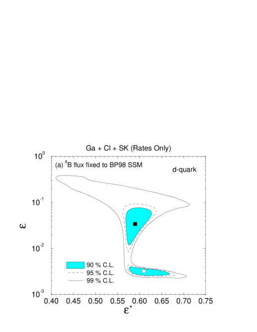
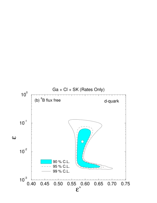
FIG. 1.: Region of $\varepsilon=\epsilon_{\nu}^{d}$ and $\varepsilon^{\prime}={\epsilon^{\prime}}_{\nu}^{d}$ which can explain the total rates measured by the Homestake, GALLEX, SAGE and SuperKamiokande solar neutrino experiments in terms of non-standard neutrino interactions with $d$-quarks. (a) The best fit (indicated by the open circle) is obtained for $(\varepsilon,\varepsilon^{\prime})=(0.0032,0.610$) with $\chi^{2}_{min}=2.44$ for $4-2=2$ DOF. A second (local) $\chi^{2}$ minimum (indicated by the solid square) is found at $(\varepsilon,\varepsilon^{\prime})=(0.034,0.610)$ with $\chi^{2}=2.63$. (b) Allowing for an arbitrary ⁸B flux normalization $f_{B}$, the best fit (indicated by the open circle) is obtained for $(\varepsilon,\varepsilon^{\prime})=(0.022,0.590)$ and $f_{B}=1.36$ with $\chi^{2}_{min}=0.91$ for $4-3=1$ DOF.

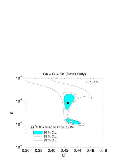
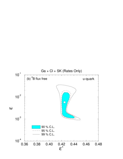
FIG. 2.: Same as in Fig. 1 but for $u$-quarks. (a) The best fit (indicated by the open circle) is obtained for $(\varepsilon,\varepsilon^{\prime})=(0.0013,0.430$) with $\chi^{2}_{min}=2.75$ for $4-2=2$ DOF. A second (local) $\chi^{2}$ minimum (indicated by the solid square) is found at $(\varepsilon,\varepsilon^{\prime})=(0.0083,0.425)$ with $\chi^{2}=2.70$. (b) Allowing for an arbitrary ⁸B flux normalization $f_{B}$, the best fit (indicated by the open circle) is obtained for $(\varepsilon,\varepsilon^{\prime})=(0.0058,0.425)$ and $f_{B}=1.34$ with $\chi^{2}_{min}=0.96$ for $4-3=1$ DOF.

FIG. 3.: The ratio of the number density of electron to that of $d$ and $u$-quarks in the sun $n_{e}(r)/n_{f}(r)$ ($f=d,u$), is plotted as a function of the distance from the solar center.

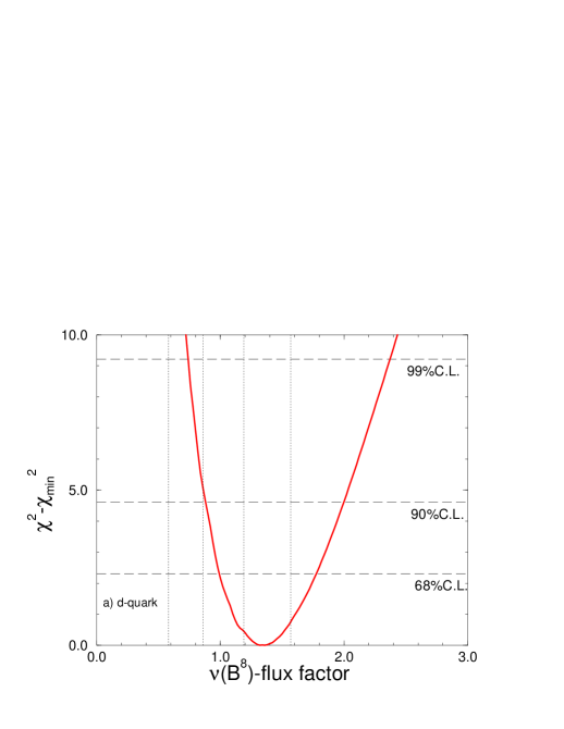
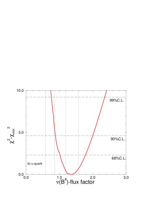
FIG. 4.: Minimum $\chi^{2}$ calculated as a function of the boron neutrino flux for (a) d-quark and (b) u-quark.

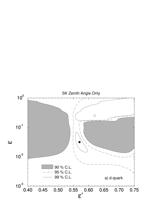
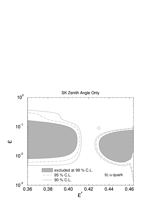
FIG. 5.: Region of $\varepsilon=\epsilon_{\nu}^{d}$ and $\varepsilon^{\prime}={\epsilon^{\prime}}_{\nu}^{d}$ which is excluded by day and night data (contained in $1+5$ bins) as measured by the SuperKamiokande solar neutrino experiment in terms of non-standard neutrino interactions with (a) $d$-quarks and (b) $u$-quarks. For $d$-quarks, the best fit (indicated by the open circle) is obtained for $(\varepsilon,\varepsilon^{\prime})=(0.251,0.620)$ and $\alpha_{Z}=0.819$ with $\chi^{2}_{min}=1.10$ for $6-3=3$ DOF. A second (local) $\chi^{2}$ minimum (indicated by the solid squared) is found at $(\varepsilon,\varepsilon^{\prime})=(0.0316,0.570$) and $\alpha_{Z}=1.02$ with $\chi^{2}=5.20$. For $u$-quarks, the best fit (indicated by the open circle) is obtained for $(\varepsilon,\varepsilon^{\prime})=(0.229,0.690)$ and $\alpha_{Z}=0.685$ with $\chi^{2}_{min}=1.44$ for $6-3=3$ DOF.

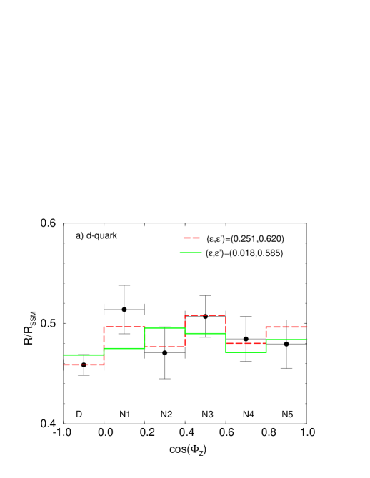
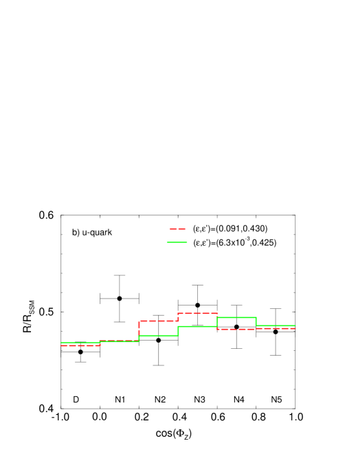
FIG. 6.: Expected the zenith angle dependence with the our best fit values of $(\varepsilon,\varepsilon^{\prime})$ determined by the SK Zenith angle only as well as the combined analysis for (a) $d$-quarks and (b) $u$-quarks.

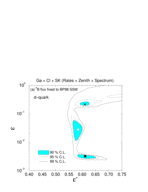
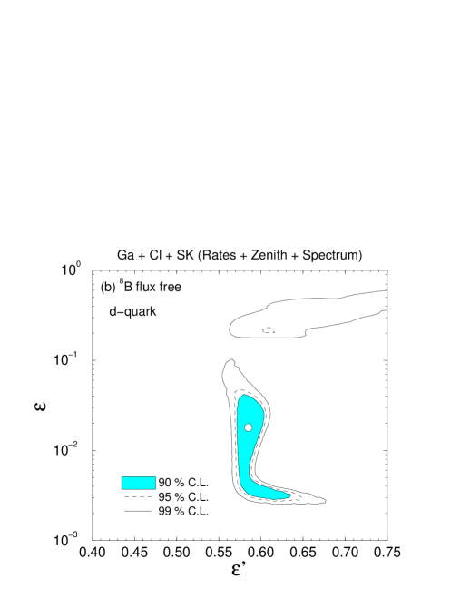
FIG. 7.: The allowed region for $\varepsilon=\epsilon_{\nu}^{d}$ and $\varepsilon^{\prime}={\epsilon^{\prime}}_{\nu}^{d}$ obtained by the combined analysis using 4 rates + 6 zenith angle bins + 18 spectrum bins for non-standard neutrino interactions with $d$-quarks. (a) Fixing $f_{B}=1$ the best fit (indicated by the open circle) is obtained for $(\varepsilon,\varepsilon^{\prime})=(0.028,0.585)$ with $\chi^{2}_{min}=29.05$ for $28-4=24$ DOF. There are two additional (local) $\chi^{2}$ minima at $(\varepsilon,\varepsilon^{\prime})=(0.0033,0.610)$ with $\chi^{2}=29.40$ (indicated by the solid square) and $(\varepsilon,\varepsilon^{\prime})=(0.21,0.61)$ with $\chi^{2}=33.1$ (indicated by the cross). (b) Same as in (a) but allowing a free $f_{B}$. The best fit (indicated by the open circle) is obtained for $(\varepsilon,\varepsilon^{\prime})=(0.018,0.585)$ and $f_{B}=1.38$ with $\chi^{2}_{min}=26.62$ for $28-5=23$ DOF.

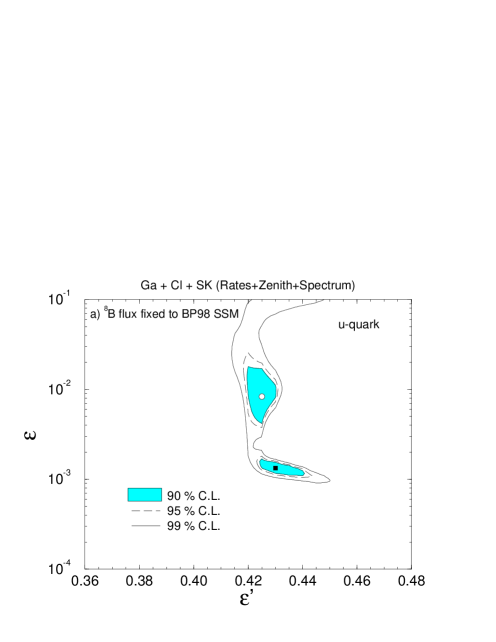
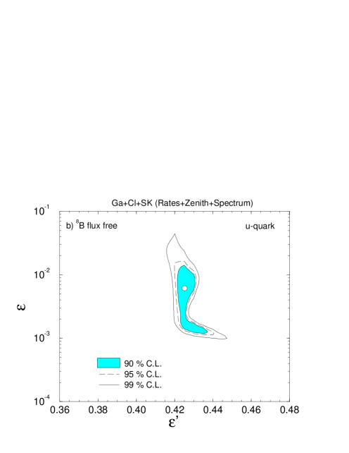
FIG. 8.: Same as in Fig. 7 but for $u$-quarks. (a) Fixing $f_{B}=1$ the best fit (indicated by the open circle) is obtained for $(\varepsilon,\varepsilon^{\prime})=(0.0083,0.425)$ with $\chi^{2}_{min}=28.45$ for $28-4=24$ DOF. A second (local) $\chi^{2}$ minimum is found at $(\varepsilon,\varepsilon^{\prime})=(0.0013,0.430)$ with $\chi^{2}=30.27$ (indicated by the solid square) (b) Same as in (a) but allowing a free $f_{B}$. The best fit (indicated by the open circle) is obtained for $(\varepsilon,\varepsilon^{\prime})=(0.0063,0.426)$ and $f_{B}=1.34$ with $\chi^{2}_{min}=26.59$ for $28-5=23$ DOF.

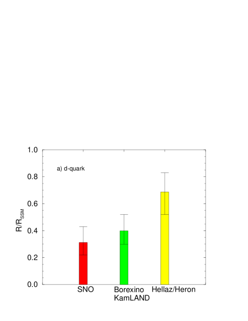
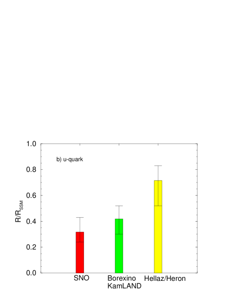
FIG. 9.: The predicted ranges of the ratios of event rates for SNO, BOREXINO and HELLAZ/HERON to the corresponding event rates predicted from the SSM assuming that the neutrino conversion induced by FCNI as well as FDNI is the solution to the solar neutrino problem. Histgrams indicate the predictions with the best fittes parameters whereas the error bars indicates the range determined by varying parameters within 95 % C.L. regions for $(\varepsilon,\varepsilon^{\prime})$ in Figs. 7b and  8b.