TUM-HEP-372/00

A consistent nonperturbative approach to thermal damping-rates

Bastian Bergerhoff and Jürgen Reingruber
Institut für Theoretische Physik
Technische Universität München
James-Franck-Strasse, D-85748 Garching, Germany

Abstract

We propose a nonperturbative scheme for the calculation of thermal damping-rates using exact renormalization group (RG)-equations. Special emphasis is put on the thermal RG where first results for the rate were given in [1]. We point out that in order to obtain a complete result that also reproduces the known perturbative behaviour one has to take into account effects that were neglected in [1]. We propose a well-defined way of doing the calculations that reproduces perturbation theory in lowest order but goes considerably beyond perturbative results and should be applicable also at second order phase-transitions.

Pacs-No.s: 11.10.Wx,11.15.Tk,05.10.Cc,05.70.Ln

Perturbation theory at finite temperatures is often invalidated by bad infrared behaviour. These problems can be solved by different resummation schemes. One of the most powerful approaches to resummation is the renormalization group of Wilson and others [2]. This involves introducing an external scale and deriving functional differential equations for the dependence of generating functionals on this scale. The right hand side of such an RG-equation can formally be interpreted as a one-loop expression in the sense that it is of order $\hbar$ compared to the left hand side. Nevertheless the Wilsonian RG constitutes a nonperturbative method and the RG-equations are exact functional relations. The approach is well known to correctly reproduce the infrared-behaviour of theories even at second-order phase-transitions.

Even though the RG-equations define a nonperturbative approach, it is possible to reproduce perturbation theory. This is straightforward for one-loop results, but becomes rather tedious if one goes to higher orders. Quantities which are well described perturbatively for a range of temperatures but for which perturbation theory fails e.g. at a phase-transition constitute a major challenge for RG-equations. This holds in particular for quantities where the one-loop contribution vanishes. The thermal damping-rate in $\varphi^{4}$-theory is an example for a quantity where the lowest order perturbative contribution is two-loop. If one aims at a reliable calculation of such quantities at all temperatures, one has to reproduce two-loop perturbation theory as the leading term and apply sensible nonperturbative resummations close to a possible phase-transition.

A recent formulation of Wilsonian RG-equations in the Schwinger-Keldysh (CTP-) formalism of real-time thermal field theory is particularily suited for calculations of nonstatic thermal Green-functions [3]. It makes use of the fact that the propagators in the CTP-formalism separate into the usual zero-temperature and a finite-T part. The finite-T parts only contribute on-shell and depend only on the three-momenta. The cutoff modifies the thermal part and one introduces cut-off propagators of the form

$$D_{\Lambda}(k) = \left(\begin{array}[]{cc}\Delta&0\\ 0&-\Delta^{*}\end{array}\right)+(\Delta-\Delta^{*})\left(\begin{array}[]{cc}0&\Theta(-k_{0})\\ \Theta(k_{0})&0\end{array}\right)+$$ (8)

$$+(\Delta-\Delta^{*})\Theta(|\vec{k}|,\Lambda)N(|k_{0}|)\left(\begin{array}[]{cc}1&1\\ 1&1\end{array}\right)$$

where $\Theta(|\vec{k}|,\Lambda)$ is a possibly smeared out step function. We will in the following use a sharp cutoff, i.e. set $\Theta(|\vec{k}|,\Lambda)=\Theta(|\vec{k}|-\Lambda)$. Thus for finite $\Lambda$, the propagation of thermal modes with three-momemtum small compared to $\Lambda$ (soft modes) is supressed, while the hard thermal modes are unmodified. Inserting this propagator into the usual expression for the generating functional $Z[J]$ one obtains a $\Lambda$-dependent functional $Z_{\Lambda}$. Introducing the modified Legendre-transform

$$\Gamma_{\Lambda}[\Phi]=-i\ln Z_{\Lambda}[J]-J\cdot\Phi-\frac{1}{2}\Phi\cdot\left(D_{\Lambda}\right)^{-1}\cdot\Phi$$ (9)

one readily obtains for the scale-dependence of $\Gamma_{\Lambda}$ the exact functional differential equation [3]

$$\Lambda\frac{\partial\Gamma_{\Lambda}[\Phi]}{\partial\Lambda}=\frac{i}{2}{\mbox{Tr}}\Lambda\frac{\partial D_{\Lambda}^{-1}}{\partial\Lambda}\left(D_{\Lambda}^{-1}+\frac{\delta^{2}\Gamma_{\Lambda}[\Phi]}{\delta\Phi\delta\Phi}\right)^{-1}$$ (10)

This is the thermal renormalization group equation (TRG) and will be the starting point of our discussion.

Being a differential equation, (10) of course has to be supplemented by boundary conditions. As discussed in [3], in the limit $\Lambda\rightarrow\infty$, the effective action $\Gamma_{\Lambda}$ is trivially obtained from the $(T\!=\!0)$-effective action of the theory. Also, in the limit $\Lambda\rightarrow 0$ the full finite temperature CTP-effective action $\Gamma[\Phi]$ is obtained.

RG-equations for Green-functions are simply obtained from (10) by taking functional derivatives with respect to $\Phi$. For the damping-rate, we are interested in the imaginary part of the two-point function. The flow-equation for the two-point function reads in terms of the thermal fields $\varphi_{i}$ with $i=1,2$ ($\varphi_{0}$ is some background configuration)

$$\left.\Lambda\frac{\partial}{\partial\Lambda}\frac{\delta^{2}\Gamma_{\Lambda}}{\delta\varphi_{i}\delta\varphi_{j}}\right|_{\varphi_{0}} = \left.\frac{1}{2}{\mbox{Tr}}K_{\Lambda}\frac{\delta^{4}\Gamma_{\Lambda}}{\delta\varphi_{i}\delta\varphi_{j}\delta\Phi\delta\Phi}\right|_{\varphi_{0}}-$$ (11)

$$\quad-\left(\left.\frac{1}{2}{\mbox{Tr}}K_{\Lambda}\frac{\delta^{3}\Gamma_{\Lambda}}{\delta\varphi_{i}\delta\Phi\delta\Phi}{\mathcal{D}}\frac{\delta^{3}\Gamma_{\Lambda}}{\delta\varphi_{j}\delta\Phi\delta\Phi}\right|_{\varphi_{0}}+(i\leftrightarrow j)\right)$$

where $K_{\Lambda}=-i{\mathcal{D}}\Lambda\frac{\partial D_{\Lambda}^{-1}}{\partial\Lambda}{\mathcal{D}}$ is the kernel of the TRG and ${\mathcal{D}}=\left(D_{\Lambda}^{-1}+\Gamma_{\Lambda}^{(2)}\right)^{-1}$ is the full two-point function [3]. Even though in this representation the flow-equation appears like a plain one-loop equation, due to the fact that all $n$-point functions involved are full $n$-point functions it is actually an exact, nonperturbative expression.

Let us then assume that we want to calculate the imaginary part of the thermal two-point function in a scalar theory with unbroken $Z_{2}$-symmetry. Perturbatively in this case the lowest contribution to the imaginary part of the self-energy occurs on two-loop level. As out in [1], in such a situation the contribution to the imaginary part of (11) has to come from an imaginary part of the full four-point function (by the $Z_{2}$-symmetry, the second contribution in (11) vanishes identically for all $\Lambda$). We thus have to solve a coupled system of at least two flow-equations, (11) and a corresponding equation for the imaginary part of the four-point function.

First however let us make some remarks concerning the thermal indice which appear in real-time formulations of thermal field-theory [4]. The physical fields always carry a thermal index 1 and one is in general interested in the calculation of Green-functions for those fields. Since the propagators are nondiagonal in the thermal indice, in the calculation of higher loop contributions one has to include vertice of the 2-fields nevertheless – neglecting those contributions yields singular expressions. If we use the TRG to compute Green-functions, we have to use full vertice according to (10). In this case, one has to allow for vertice with mixed thermal structure.

Furthermore, what enters the physical self-energy (and thus the damping-rate) is not the Green-function $\frac{\delta^{2}\Gamma}{\delta\varphi_{1}\delta\varphi_{1}}$, but rather a specific combination of the $\frac{\delta^{2}\Gamma}{\delta\varphi_{i}\delta\varphi_{j}}$ [4], known as $\bar{\Pi}(p)$ in the literature. Assuming a Schwinger-Dyson equation for the full propagator it is easy to show that for the real- and imaginary parts of $\bar{\Pi}$ the following relations hold:

$${\mathcal{R}}\bar{\Pi}(p) = {\mathcal{R}}\frac{\delta^{2}\Gamma}{\delta\varphi_{1}(p)\delta\varphi_{1}(-p)}$$

$${\mathcal{I}}\bar{\Pi}(p) = \epsilon(p_{0}){\mathcal{I}}\left(\frac{\delta^{2}\Gamma}{\delta\varphi_{1}(p)\delta\varphi_{1}(-p)}+\frac{\delta^{2}\Gamma}{\delta\varphi_{1}(p)\delta\varphi_{2}(-p)}\right)$$ (12)

($\epsilon(p_{0})$ is the sign function). ${\mathcal{I}}\bar{\Pi}$ can also be obtained as

$${\mathcal{I}}\bar{\Pi}(p) = \frac{1}{1+2N(|p_{0}|)}{\mathcal{I}}\frac{\delta^{2}\Gamma}{\delta\varphi_{1}(p)\delta\varphi_{1}(-p)}$$ (13)

Note that this expression explicitely involves a distribution function, whereas the second equation of (12) does not. We will below use (12) for a calculation of the physical self-energy. Another important feature of real-time thermal field-theories is that the effective action has the following symmetry [5]

$$\Gamma[\varphi_{1},\varphi_{2}]=-\Gamma^{*}[\varphi_{2}^{*},\varphi_{1}^{*}]$$ (14)

For real, momentum independent vertice (in the present theory with a real scalar field in configuration space), this gives the following relations:

$$\Gamma^{(n)}_{i_{1}i_{2}...i_{n}}=-\Gamma^{(n)}_{\bar{i}_{1}\bar{i}_{2}...\bar{i}_{n}}$$ (15)

where $\bar{i}=2$ for $i=1$ and vice versa. Furthermore one may introduce a functional $\bar{\Gamma}[\phi]$ by

$$\frac{\delta\bar{\Gamma}[\phi]}{\delta\phi}=\left.\frac{\delta\Gamma}{\delta\varphi_{1}}\right|_{\varphi_{1}=\phi,\varphi_{2}=\varphi_{2}[\phi]}$$ (16)

where $\varphi_{2}[\phi]$ is the solution of the field-equation for $\varphi_{2}$. For momentum-independent vertice, it is easy to see that one has

$$\bar{\Gamma}^{(3)}=\sum_{i,j=1,2}\left.\Gamma^{(3)}_{1ij}\right|_{\varphi_{a}=\phi}\quad;\quad\bar{\Gamma}^{(4)}=\sum_{i,j,k=1,2}\left.\Gamma^{(4)}_{1ijk}\right|_{\varphi_{a}=\phi}$$ (17)

and so on. These relations trivially generalize to $\Gamma_{\Lambda}$ and we will make use of them below.

Let us now turn to the calculation of the imaginary part of the self-energy of (at $T\!=\!0$) massless $\varphi^{4}$-theory. In order to obtain an equation for the scale-dependence of ${\mathcal{I}}\bar{\Pi}$, we plug the flow-equations for the two-point functions with 1-1 and 1-2 external legs into the second relation in (12). We now make a crucial approximation: We neglect the imaginary part of the self-energy on the right hand side of all flow-equations (for the present work we also assume ${\mathcal{R}}\bar{\Pi}$ to be momentum-independent, which is however not crucial for the results discussed and could be straightforwardly improved). This may be viewed as a ”quasiparticle-approximation”. As we will see below, it does not influence the leading behaviour for small couplings. Making this approximation however means that we will not be resumming imaginary parts in the calculations – a fact important to keep in mind.

In this case, the kernel takes the form [3]

$$K_{\Lambda}(k) = -2\pi\delta(k^{2}-m_{\Lambda}^{2})\Lambda\delta(|\vec{k}|-\Lambda)N(|k_{0}|)\left(\begin{array}[]{cc}1&1\\ 1&1\end{array}\right)$$ (20)

($m_{\Lambda}$ is the real part of the self-energy) and is purely real. It is thus immediatly clear that all contributions to the flow of ${\mathcal{I}}\bar{\Pi}$ are from the imaginary part of the full four-point function. Also, due to the specific combination of $\Gamma_{\Lambda,11}^{(2)}$ and $\Gamma_{\Lambda,12}^{(2)}$ appearing in (12), taking the trace over thermal indice in the flow-equation for $\bar{\Pi}$ leaves us with the following result:

$$\Lambda\frac{\partial{\mathcal{I}}\bar{\Pi}_{\Lambda}\!(p)}{\partial\Lambda}=-\frac{\Lambda^{3}}{4\pi^{2}}\frac{N(\omega_{\Lambda})}{\omega_{\Lambda}}\epsilon(p_{0})\!\!\!\sum_{i,j,k=1,2}\!\!\!{\mathcal{I}}\Gamma_{\Lambda,1ijk}^{(4)}(p,\!-p,Q_{\Lambda},\!-Q_{\Lambda})$$ (21)

In (21) we use the notation

$$\omega_{\Lambda}=\sqrt{\Lambda^{2}+m_{\Lambda}^{2}}\quad,\quad Q_{\Lambda}=(\omega_{\Lambda},|\vec{Q_{\Lambda}}|=\Lambda)$$ (22)

For the quantities appearing on the right hand side of (21), we again need the RG-equations governing their scale-dependence. Let us first discuss the flow-equation for the coupling appearing in (21). We use the notation

$${\mathcal{I}}\!\!\!\!\sum_{i,j,k=1,2}\!\!\!\Gamma_{\Lambda,1ijk}^{(4)}(p,-p,q,-q)={\mathcal{I}}\bar{\Gamma}_{\Lambda}^{(4)}(p,-p,q,-q)$$ (23)

which is suggested by (17). We now make a further approximation, which is on equal footing with the quasiparticle-approximation done above: We neglect the imaginary parts of all couplings on the right hand side of the flow-equation for ${\mathcal{I}}\bar{\Gamma}^{(4)}_{\Lambda}$. This should of course not be done in (21), since there one would disregard the leading (and in fact only) contribution. Within this approximation we find:

$$\Lambda\frac{\partial}{\partial\Lambda}{\mathcal{I}}\bar{\Gamma}_{\Lambda}^{(4)}(p,-p,q,-q)\!\!\! = \!\!\!-\frac{\Lambda}{2}\left(\bar{\Gamma}^{(4)}_{\Lambda}\right)^{2}\int\!\!\frac{d^{4}l}{(2\pi)^{2}}\delta(l^{2}\!-\!m_{\Lambda}^{2})\theta(|\vec{l}|^{2}\!+\!m_{\Lambda}^{2})\delta(|\vec{l}|\!-\!\Lambda)N(|l_{0}|)\!\!\times$$ (24)

$$\qquad\qquad\qquad\times\sum_{Q=\pm q}\delta((l+p+Q)^{2}-m_{\Lambda}^{2})\epsilon(l_{0}+p_{0}+Q_{0})$$

Note that (24) is a completely well-defined expression. Furthermore the vertex appearing here is just the combination defined in (17), and we have taken into account vertice with both 1- and 2-external legs. This is only possible for the specific sum in (23). Neglecting vertice with 2-legs within the present approach would yield ill-defined products of distributions. We have checked that the inclusion of trilinear couplings in the present approximations (i.e. considering a theory with broken symmetry at low temperatures) is possible along the same line of arguments. Thus the results depicted in (21) and (24), together with a flow-equation for the real part of the effective action at constant fields, constitute a well-defined nonperturbative method for the calculation of thermal rates. This is the first important point in the present work.

Even though the approach using Wilsonian RG-equations is nonperturbative one wants to recover the leading perturbative results in situations where perturbation theory is valid. This is a nontrivial problem, since ${\mathcal{I}}\bar{\Pi}$ in the theory under study vanishes to one-loop order.

The loop expansion can be reconstructed from Wilsonian RG-equations iteratively, making use of the fact that the right hand side of (10) is down by a factor of $\hbar$ compared to the left hand side. In order to obtain a result for ${\mathcal{I}}\bar{\Pi}$ to order $\hbar^{2}$, we need the right hand side of (21) to order $\hbar$. The quantities appearing on the right hand side of (21) are the thermal mass $m_{\Lambda}$ and the imaginary part of the four-point function at finite $\Lambda$. This imaginary part is a pure quantum effect and thus is itself of order $\hbar$, so we need not consider corrections to the mass.

In order to find the imaginary part of the four-point function (which has to be calculated for the specific choice of momenta entering in (21) and at nonvanishing external scale $\Lambda$), we turn to the corresponding flow-equation (24). To order $\hbar$ we may neglect all loop corrections to the quantities appearing on the right hand side of (24). Thus to this order the couplings and masses are $\Lambda$-independent and the integration of (24) may be performed noting that $-\delta(|\vec{l}|-\Lambda)=\partial_{\Lambda}\theta(|\vec{l}|-\Lambda)$. One finds

$${\mathcal{I}}\bar{\Gamma}_{\Lambda}^{(4)}(p,-p,q,-q)={\mathcal{I}}\bar{\Gamma}_{\Lambda=\infty}^{(4)}(p,-p,q,-q)+$$

$$\quad+\frac{1}{2}\left(\bar{\Gamma}^{(4)}\right)^{2}\!\!\int\!\!\frac{d^{4}l}{(2\pi)^{2}}\delta(l^{2}\!-\!m^{2})\theta(|\vec{l}|^{2}\!+\!m^{2})\theta(|\vec{l}|\!-\!\Lambda)N(|l_{0}|)\!\!\times$$

$$\qquad\quad\times\sum_{Q=\pm q}\delta((l+p+Q)^{2}-m^{2})\epsilon(l_{0}+p_{0}+Q_{0})$$ (25)

Plugging this result into the right hand side of the flow-equation for ${\mathcal{I}}\bar{\Pi}$ and performing the remaining $\Lambda$-integration should then give the desired imaginary part of the self energy to order $\hbar^{2}$.

The result of a perturbative calculation may be taken e.g. from [6] where one finds

$${\mathcal{I}}\bar{\Pi}(p)=-\pi\epsilon(p_{0})\frac{\left(\bar{\Gamma}^{(4)}\right)^{2}}{6}\int\frac{d^{3}\vec{k}}{(2\pi)^{3}}\frac{d^{3}\vec{q}}{(2\pi)^{3}}\frac{1}{8\omega_{k}\omega_{q}\omega_{r}}\times$$

$$\qquad\times\biggl{\{}\left[\delta(p_{0}\!+\!\omega_{k}\!+\!\omega_{q}\!+\!\omega_{r})-\delta(p_{0}\!-\!\omega_{k}\!-\!\omega_{q}\!-\!\omega_{r})\right]\times$$

$$\qquad\qquad\qquad\qquad\times\left[1\!+\!N_{k}\!+\!N_{q}\!+\!N_{r}\!+\!N_{k}N_{q}\!+\!N_{k}N_{r}\!+\!N_{q}N_{r}\right]+$$

$$\qquad\qquad+\left[\delta(p_{0}\!+\!\omega_{k}\!+\!\omega_{q}\!-\!\omega_{r})-\delta(p_{0}\!-\!\omega_{k}\!-\!\omega_{q}\!+\!\omega_{r})\right]\left[N_{r}\!+\!N_{k}N_{r}\!+\!N_{q}N_{r}\!-\!N_{k}N_{q}\right]+$$

$$\qquad\qquad+\left[\delta(p_{0}\!+\!\omega_{k}\!-\!\omega_{q}\!+\!\omega_{r})-\delta(p_{0}\!-\!\omega_{k}\!+\!\omega_{q}\!-\!\omega_{r})\right]\left[N_{q}\!+\!N_{k}N_{q}\!+\!N_{r}N_{q}\!-\!N_{k}N_{r}\right]+$$

$$\qquad\qquad+\left[\delta(p_{0}\!-\!\omega_{k}\!+\!\omega_{q}\!+\!\omega_{r})-\delta(p_{0}\!+\!\omega_{k}\!-\!\omega_{q}\!-\!\omega_{r})\right]\left[N_{k}\!+\!N_{k}N_{q}\!+\!N_{k}N_{r}\!-\!N_{q}N_{r}\right]\biggr{\}}$$ (26)

where again $\omega_{p}=\sqrt{\vec{p}^{2}+m^{2}}$ and $\vec{r}=\vec{k}+\vec{q}+\vec{p}$. $N_{p}$ is the Bose-distribution with energy $\omega_{p}$. The part $\propto 1$ is of course the $(T\!=\!0)$-imaginary part. In the present method this part enters via the boundary conditions and is not calculable within the TRG. The other parts however have to come out of our result from (21) and (24).

An important observation at this point is that for the one-loop contribution in (25) one has two parts, one being the boundary part at $\Lambda\!=\!\infty$ which is given by the one-loop $(T\!=\!0)$-result and the second one being proportional to $N$ and representing the contribution from thermal fluctuations. If we simply start with the tree-level effective action at $T\!=\!0$ – that is set the imaginary part of the four point function to 0 for $\Lambda\rightarrow\infty$ – and plug the remaining contribution from (25) into (21), we only reproduce the contributions to ${\mathcal{I}}\bar{\Pi}$ which are bilinear in the distribution functions. Dropping all $(T\!=\!0)$-quantum contributions for the boundary value of the flow of $n$-point functions is however routinely done in applications of the TRG ([1, 3, 7, 8, 9]). Since the thermal damping-rate vanishes to one-loop, one does not reproduce the leading order perturbative result (26) and will not be able to give quantitatively reliable results for all temperatures.

To end the discussion of the perturbative result, we thus need the $\Lambda\rightarrow\infty$ or $(T\!=\!0)$-value of the imaginary part of the four-point function to one loop. This is easily found to be

$${\mathcal{I}}\bar{\Gamma}_{\Lambda=\infty}^{(4)}(p,-p,q,-q)\!\! = \!\!\sum_{Q=\pm q}\!\frac{\pi}{8}\left(\bar{\Gamma}_{T=0}^{(4)}\right)^{2}\!\int\!\!\frac{d^{3}\vec{k}}{(2\pi)^{3}}\frac{1}{\omega_{k}\omega_{k+p+Q}}\times$$ (27)

$$\quad\times\left[\delta(p_{0}\!+\!Q_{0}\!-\!\omega_{k}\!-\!\omega_{k+p+Q})-\delta(p_{0}\!+\!Q_{0}\!+\!\omega_{k}\!+\!\omega_{k+p+Q})\right]$$

Using this result in (25) and plugging the resulting expression for ${\mathcal{I}}\bar{\Gamma}_{\Lambda}^{(4)}(p,-p,Q_{\Lambda},-Q_{\Lambda})$ into the flow-equation for ${\mathcal{I}}\bar{\Pi}(p)$ given in (21) one may indeed do the integration with respect to $\Lambda$ to find for $\Lambda=0$ the perturbative result (26) up to its $(T\!=\!0)$-part.

In order to go beyond the leading order two-loop result, we will take into account the thermal renormalization of the real parts of both the self-energy as well as the momentum-independent parts of the vertice. We perform a derivative expansion of the full effective action $\bar{\Gamma}_{\Lambda}$ and approximate it by the effective potential and a standard kinetic term. This approximation is discussed in detail in [3, 7, 8, 9] where also the resulting flow-equations may be found. We solve the flow-equation for the effective potential as discussed in [7, 8, 9] and thus resum the momentum-independent (thermal) parts of $n$-point functions with an arbitrary number of external legs – this resummation goes considerably beyond the usual daisy- or superdaisy-resummations. It can be systematically improved by relaxing the derivative-approximation.

As the boundary condition for the flow of the effective potential we will use the tree-level effective potential of a massless $\varphi^{4}$-theory, $U_{\Lambda=\infty}=\frac{g_{T=0}}{24}\phi^{2}$. This amounts to neglecting all $(T\!=\!0)$-loop corrections to the effective potential. Together with the boundary conditions and flow-equations for the imaginary parts as discussed above we thus have a closed system of differential equations which may be solved numerically.

The resulting imaginary part of the self-energy is connected to the thermal damping-rate $\gamma(T)$ through

$$\gamma(T)=\frac{{\mathcal{I}}\bar{\Pi}_{\Lambda=0}(p_{0}=m_{T},\vec{p}=0)}{2m_{T}}$$ (28)

Perturbatively, using daisy-resummed perturbation theory one finds for a massless theory [6, 10, 11]

$$\gamma_{pert}(T)=\frac{g_{T=0}^{3/2}}{64\sqrt{24}\pi}\sqrt{1-\frac{3g_{T=0}^{1/2}}{\sqrt{24}\pi}}T$$ (29)

In figure 1 we display the ratio of the result obtained using the flow-equations and (29) as a function of $g_{T=0}$. Indeed the TRG reproduces daisy-resummed perturbation theory for $g_{T=0}\rightarrow 0$, even though the leading perturbative result is two-loop. For finite values of the coupling, the different resummations yield different results. Let us again point out that the result of the renormalization group-calculations performed here can be understood as a fully resummed result in leading order in an expansion in the anomalous dimension and the quasiparticle approximation. It goes beyond the resummations used in the literature (it in particular trivially includes the daisy- and superdaisy-schemes [3]).

Figure 2 shows the dependence of the real- and imaginary parts of the self-energy on the external scale $\Lambda$ at fixed $g_{T=0}$. We note the typical behaviour: Small corrections to the $(T\!=\!0)$-values for large $\Lambda/T$ due to Boltzmann-suppression of the thermal fluctuations and saturation of the values for $\Lambda\ll m_{\Lambda}$. The limit $\Lambda\rightarrow 0$ is completely safe.

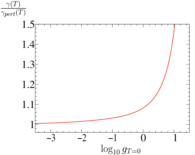
Figure 1: $\gamma(T)/\gamma_{pert}(T)$ as function of $\log g_{T=0}$.

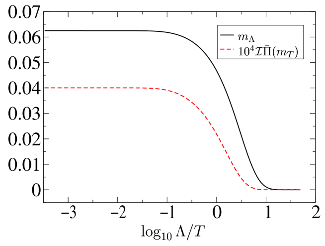
Figure 2: The thermal mass $m_{\Lambda}$ and the imaginary part of the self energy ${\mathcal{I}}\bar{\Pi}_{\Lambda}(m_{T})$ as functions of $\log\Lambda/T$. $g_{T=0}=0.1$ was chosen and dimensionful quantities are in units of $T$.

We close this letter by commenting on one of the most important qualitative points made in [1], namely that a calculation of the damping-rate from the TRG reproduces critical slowing down, i.e. the fact that the rate vanishes as the critical temperature of a theory with (at $T\!=\!0$) spontaneously broken $Z_{2}$-symmetry is approached. We believe that even though this conclusion was reached on the basis of an incomplete calculation it still holds if one uses the consistent approach laid out in the present paper. The reason why this should be the case is easy to see: The rate is an on-shell quantity with vanishing external momentum and as the critical temperature of the (second-order) phase-transition is approached, the external energy thus vanishes. On the other hand, in the framework of Wilsonian RG-equations internal propagators are never massless for any $\Lambda>0$. Close to the phase-transition, the masses and coupling exhibit three-dimensional scaling behaviour, i.e. the renormalized mass and coupling vanish as

$$m_{T}\propto(T-T_{c})^{\nu}\quad;\quad g_{T}\propto(T-T_{c})^{\nu}$$ (30)

In such a case, the limit $m_{T}\rightarrow 0$ should be completely regular and the scaling arguments also given in [1] should still hold: The perturbative result for the imaginary part of the self-energy behaves for small $m_{T}$ as $\bar{\Pi}(m_{T},0)\sim g_{T=0}^{2}\ln m_{T}$ and thus one has for the rate

$$\gamma(T)\sim\frac{g_{T=0}^{2}}{m_{T}}\ln m_{T}$$ (31)

Consistent resummation using the Wilsonian RG replaces the coupling $g_{T=0}$ with the renormalized coupling $g_{T}$ and one obtains with $t=T-T_{c}$

$$\gamma(T\rightarrow T_{c})\propto t^{\nu}\ln t\rightarrow 0$$ (32)

for positive $\nu$ (in the present model, $\nu$ is found to be $\sim 0.63$ [12, 8, 9]).

Within the scheme presented here we now have for the first time a complete approach that allows us to study linear-response and static quantities in a nonperturbative manner also in the critical regime, while reproducing the perturbative results where they are valid. As shown in [9], the TRG can also be formulated for theories involving fermionic degrees of freedom. It should be very interesting to apply this nonperturbative method e.g. to questions related to the physics of nuclear matter as the chiral phase-transition is approached.

Acknowledgements: We thank M. Pietroni for helpful discussions on his results.

References

- [1] M. Pietroni, Phys. Rev. Lett. 81 (1998), 2424.
- [2] K.G. Wilson and J.G. Kogut, Phys. Rep. 12 (1974) 75.
- [3] M. D’Attanasio and M. Pietroni, Nucl. Phys. B472 (1996) 711.
- [4] M. Le Bellac, ”Thermal Field Theory” (Cambridge 1996).
- [5] A. Niemi and G. Semenoff, Ann. of Phys. 152 (1984) 105.
- [6] E. Wang and U. Heinz, Phys. Rev. D53 (1996), 899.
- [7] B. Bergerhoff, Phys. Lett. B437 (1998), 381.
- [8] B. Bergerhoff and J. Reingruber, Phys. Rev. D60 (1999), 105036.
- [9] B. Bergerhoff, J. Manus and J. Reingruber, hep-ph/9912474, to appear in Phys. Rev. D.
- [10] R.R. Parwani, Phys. Rev. D45 (1992), 4695, D48 (1993), 5965 (E).
- [11] S. Jeon, Phys. Rev. D52 (1995), 3591.
- [12] J. Zinn-Justin, ”Quantum Field Theory and Critical Phenomena” (Oxford 1989).