Variable number schemes for heavy quark electroproduction

Abstract

We compare variable number schemes for heavy quark electroproduction.

Heavy quark production has been a major topic of investigation at hadron-hadron, electron-proton and electron-positron colliders. Here a review is given of some topics which are of interest primarily for electron-proton colliders. We concentrate on this reaction because a theoretical treatment can be based on the operator product expansion, and also because data are available for deep-inelastic charm production at HERA. How all this relates to Fermilab experiments will be discussed at the end.

In QCD perturbation theory one needs to introduce a renormalization scale and a mass factorization scale to perform calculations. We choose both equal to $\mu^{2}$, which will be a function of $Q^{2}$ and the square of the mass of the charm quark $m^{2}$. At small $\mu^{2}$, where kinematic effects due to quark masses are important, the best way to describe charm quark production is via heavy quark pair production where parton densities are used for the initial state light mass u,d,s quarks and the gluon and $m$ only appears in the heavy quark coefficient functions (or partonic cross sections) like $H_{i,g}^{\rm S,(2)}(z,Q^{2},m^{2},\mu^{2})$, etc., [1]. Here the superscripts refer to their flavor decomposition and the order in perturbation theory, while the subscripts refer to the projection $i=2,L$ and the partonic initial state. The arguments refer to the partonic Bjorken variable $z=Q^{2}/(s+Q^{2})$ and to the fact that these functions depend upon invariants and scales. The renormalization necessary to calculate these NLO expressions follows the CWZ method [2]. The symbol $H$ refers to those coefficient functions which are derived from Feynman diagrams where the virtual photon couples to a heavy quark line. Analytic expressions for these functions are not known. Numerical fits are available in [3]. Asymptotic expressions for $Q^{2}\gg m^{2}$ are available in [4] which contain terms like $\ln^{2}(Q^{2}/m^{2})$ and $\ln(Q^{2}/m^{2})\ln(Q^{2}/\mu^{2})$ multipled by functions of $z$ and demonstrate that these functions are singular in the limit that $m\rightarrow 0$. There are other heavy quark coefficient functions such as $L_{i,q}^{\rm NS,(2)}(z,Q^{2},m^{2})$, which arise from tree diagrams where the virtual photon attaches to the an initial state light quark line, so the heavy-quark is pair produced via virtual gluons. Analytic expressions for these functions are known for all $z$, $Q^{2}$ and $m^{2}$, which, in the limit $Q^{2}\gg m^{2}$ contain powers of $\ln(Q^{2}/m^{2})$ multiplied by functions of $z$. The three-flavor light mass $\overline{\rm MS}$ parton densities can be defined in terms of matrix elements of operators and are now available in parton density sets. This is a fixed order perturbation theory (FOPT) description of heavy quark production with three-flavour parton densities. Notice that due to the work in [1] the perturbation series is now known up to second order. In regions of moderate scales and invariants this NLO description is well defined and can be combined with a fragmentation function to predict exclusive distributions [5] for the outgoing charm meson, the anti-charm meson and the additional parton. This NLO massive charm approach agrees well with the recent $D$-meson inclusive data in [6] and [7]. Let us call the charm quark structure functions in this NLO description $F^{\rm EXACT}_{i,c}(x,Q^{2},m^{2},n_{f}=3)$, where $i=2,L$.

A different description, which should be more appropriate for large scales, where terms in $m^{2}$ are negligible, is to represent charm production by a parton density $f_{c}(x,\mu^{2})$, with a boundary condition that the density vanishes at small values of $\mu^{2}$. Although at first sight these approaches are completely different they are actually intimately related. It was shown in [8] that the large terms in $\ln(Q^{2}/m^{2})$ which arise when $Q^{2}\gg m^{2}$, can be resummed in all orders in perturbation theory. In this reference all the two-loop corrections to the matrix elements of massive quark and massless gluon operators in the operator product expansion were calculated. These contain the same type of logarithms mentioned above multiplied by functions of $z$, (which is the last Feynman integration parameter). After operator renormalization and suitable reorganization of convolutions of the operator matrix elements (OME’s) and the coefficient functions the expressions for the infrared-safe charm quark structure functions $F_{i,c}(x,Q^{2},m^{2},\Delta)$, become, after resummation, convolutions of light mass four-flavor parton coefficient functions, commonly denoted by expressions like ${\cal C}^{\rm S,(2)}_{i,g}(Q^{2}/\mu^{2})$ (available in [9], [10]), with four-flavor light parton densities, which also include a charm quark density $f_{c}(x,\mu^{2})$. Since the corrections to the OME’s contain terms in $\ln(Q^{2}/m^{2})$ and $\ln(m^{2}/\mu^{2})$ as well as nonlogarithmic terms it is simplest to work in the $\overline{\rm MS}$ scheme with the scale $\mu^{2}=m^{2}$ for $Q^{2}\leq m^{2}$ and $\mu^{2}=m^{2}+Q^{2}(1-m^{2}/Q^{2})^{2}/2$ for $Q^{2}>m^{2}$ and discontinuous matching conditions on the flavor densities at $\mu^{2}=m^{2}$. Then all the logarithmic terms vanish at $Q^{2}=\mu^{2}=m^{2}$ and the non-logarithmic terms in the OME’s are absorbed into the boundary conditions on the charm density, the new four-flavor gluon density and the new light-flavor u,d,s densities. The latter are convolutions of the previous three-flavor densities with the OME’s given in the Appendix of [8]. Hence we have a precise description through order $\alpha_{s}^{2}$ of how, in the limit $m\rightarrow 0$, to reexpress the $F_{i,c}^{\rm EXACT}(x,Q^{2},m^{2})$ written in terms of convolutions of heavy quark coefficient functions with three-flavor light parton densities into a description in terms of four-flavor light-mass parton coefficient functions convoluted with four-flavor parton densities. This procedure leads to the so-called zero mass variable flavor number scheme (ZM-VFNS) for $F_{i,c}(x,Q^{2},\Delta)$ where the $m$ dependent logarithms are absorbed into the new four-flavor densities. To implement this scheme one has to be careful to use inclusive quantities which are collinearly finite in the limit $m\rightarrow 0$ and $\Delta$ is an appropriate parameter which enables us to do this. In the expression for $F_{i,c}$ there is a cancellation of terms in $\ln^{3}(Q^{2}/m^{2})$ between the two-loop corrections to the light quark vertex function (the Sudakov form factor) and the convolution of the densities with the soft part of the $L_{2,q}$-coefficient function. This is the reason for the split of $L_{i,q}$ into soft and hard parts, via the introduction of a constant $\Delta$. Details and analytic results for $L_{i,c}^{\rm SOFT}$ and $L_{i,c}^{\rm HARD}$ are available in [11]. All this analysis yielded and used the two-loop matching conditions on variable-flavor parton densities across flavor thresholds, which are special scales where one makes transitions from say a three-flavor massless parton scheme to a four-flavor massless parton scheme. The threshold is a choice of $\mu$ which has nothing to do with the actual kinematical heavy flavour pair production threshold at $Q^{2}(x^{-1}-1)=4m^{2}$. In [8],[12] it was shown that the $F^{\rm EXACT}_{i,c}(x,Q^{2},m^{2},n_{f}=3)$ tend numerically to the known asymptotic results in $F^{\rm ASYMP}_{i,c}(x,Q^{2},m^{2},n_{f}=3)$, when $Q^{2}\gg m^{2}$, which also equal the ZM-VFNS results, which were called $F^{\rm PDF}_{i,c}(x,Q^{2},n_{f}=4)$. The last description is good for large (asymptotic) scales and contains a charm density $f_{c}(x,\mu^{2})$ which satisfies a specific boundary condition at $\mu^{2}=m^{2}$.

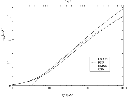
Figure 1: The charm quark structure functions $F_{2,c}^{\rm EXACT}(n_{f}=3)$ (solid line) $F_{2,c}^{\rm CSN}(n_{f}=4)$, (dot-dashed line) $F_{2,c}^{\rm BMSN}(n_{f}=4)$, (dashed line) and $F_{2,c}^{\rm PDF}(n_{f}=4)$, (dotted line) in NNLO for $x=0.005$ plotted as functions of $Q^{2}$.

s most of the experimental data occur in the kinematical regime between small $Q^{2}$ and asymptotic $Q^{2}$ a third approach has been introduced to describe the charm components of $F_{i}(x,Q^{2})$. This is called a variable flavor number scheme (VFNS). A first discussion was given in [13], where a VFNS prescription called ACOT was given in lowest order only. A proof of factorization to all orders was recently given in [14] for the total structure functions $F_{i}(x,Q^{2})$, but the NLO expressions for $F_{i,c}(x,Q^{2},m^{2})$ in this scheme were not provided. An NLO version of a VFNS scheme has been introduced in [11] and will be called the CSN scheme. A different approach, also generalized to all orders, was given in [8],[12], which is called the BMSN scheme. Finally another version of a VFNS was presented in [15], which is called the TR scheme. The differences between the various schemes can be attributed to two ingredients entering the construction of a VFNS. The first one is the mass factorization procedure carried out before the large logarithms can be resummed. The second one is the matching condition imposed on the charm quark density, which has to vanish in the threshold region of the production process. All VFNS approachs require two sets of parton densities. One set contains three-flavor number densities whereas the second set contains four-flavor number densities. The sets have to satisfy the $\overline{\rm MS}$ matching relations derived in [8]. Appropriate four-flavor densities have been constructed in [11] starting from the three-flavor LO and NLO sets of parton densities recently published in [16].

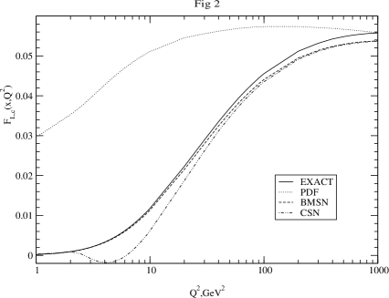
Figure 2: The charm quark structure functions $F_{L,c}^{\rm EXACT}(n_{f}=3)$ (solid line) $F_{L,c}^{\rm CSN}(n_{f}=4)$, (dot-dashed line) $F_{L,c}^{\rm BMSN}(n_{f}=4)$, (dashed line) and $F_{L,c}^{\rm PDF}(n_{f}=4)$, (dotted line) in NNLO for $x=0.005$ plotted as functions of $Q^{2}$.

Since the formulae for the heavy quark structure functions are available in [11] we only mention a few points here. The BMSN scheme avoids the introduction of any new coefficient functions other than those above. Since the asymptotic limits for $Q^{2}\gg m^{2}$ of all the operator matrix elements and coefficient functions are known we define (here $Q$ refers to the heavy charm quark)

$$F_{i,Q}^{\rm BMSN}(x,Q^{2},m^{2},\Delta,n_{f}=4)=$$

$$F_{i,Q}^{\rm EXACT}(x,Q^{2},m^{2},\Delta,n_{f}=3)$$

$$-F_{i,Q}^{\rm ASYMP}(x,Q^{2},m^{2},\Delta,n_{f}=3)$$

$$+F_{i,Q}^{\rm PDF}(x,Q^{2},m^{2},\Delta,n_{f}=4)\,.$$ (1)

The scheme for $F_{i,Q}^{\rm CSN}$ introduces a new heavy quark OME $A_{QQ}^{\rm NS,(1)}(z,\mu^{2}/m^{2})$ [17] and coefficient functions $H_{i,Q}^{\rm NS,(1)}(z,Q^{2}/m^{2})$ [18] because it requires an incoming heavy quark $Q$, which did not appear in the NLO corrections in [1]. The CSN coefficient fuctions are defined via the following equations. Up to second order we have

$${\cal C}_{i,q,Q}^{\rm CSN,SOFT,NS,(2)}\Big{(}\Delta,\frac{Q^{2}}{m^{2}},\frac{Q^{2}}{\mu^{2}}\Big{)}=$$

$$A_{qq,Q}^{\rm NS,(2)}\Big{(}\frac{\mu^{2}}{m^{2}}\Big{)}{\cal C}_{i,q}^{\rm NS,(0)}-\beta_{0,Q}\ln\left(\frac{\mu^{2}}{m^{2}}\right)$$

$$\times{\cal C}_{i,q}^{\rm NS,(1)}\Big{(}\frac{Q^{2}}{\mu^{2}}\Big{)}-{\cal C}_{i,q}^{\rm VIRT,NS,(2)}(\frac{Q^{2}}{m^{2}})$$

$$-L_{i,q}^{\rm SOFT,NS,(2)}\Big{(}\Delta,\frac{Q^{2}}{m^{2}},\frac{Q^{2}}{\mu^{2}}\Big{)}\,,$$ (2)

with the virtual term the second order Sudakov form factor. The other CSN coefficient functions are defined by equations like (we only give one of the longitudinal terms for illustration)

$${\cal C}_{L,g}^{\rm CSN,S,(1)}\Big{(}\frac{Q^{2}}{m^{2}},\frac{Q^{2}}{\mu^{2}}\Big{)}=$$

$$H_{L,g}^{\rm S,(1)}\Big{(}\frac{Q^{2}}{m^{2}}\Big{)}-A_{Qg}^{\rm S,(1)}(\frac{\mu^{2}}{m^{2}})\,{\cal C}_{L,Q}^{\rm CSN,NS,(0)}\Big{(}\frac{Q^{2}}{m^{2}}\Big{)}\,,$$ (3)

with ${\cal C}_{L,Q}^{\rm CSN,NS,(0)}={4m^{2}}/{Q^{2}}$. The CSN and BMSN schemes are designed to have the following two properties. First of all, suppressing unimportant labels,

$$F_{i,Q}^{\rm CSN}(n_{f}=4)=F_{i,Q}^{\rm BMSN}(n_{f}=4)=$$

$$F_{i,Q}^{\rm EXACT}(n_{f}=3)\quad\mbox{for}\quad Q^{2}\leq m^{2}\,.$$ (4)

Since $f_{Q}(m^{2})^{\rm NNLO}\not=0$ (see [8]) this condition can be only satisfied when we truncate the perturbation series at the same order. The second requirement is that

$$\mathop{\mbox{lim}}\limits_{\vphantom{\frac{A}{A}}Q^{2}\gg m^{2}}F_{i,Q}^{\rm BMSN}(n_{f}=4)=$$

$$\mathop{\mbox{lim}}\limits_{\vphantom{\frac{A}{A}}Q^{2}\gg m^{2}}F_{i,Q}^{\rm CSN}(n_{f}=4)=\mathop{\mbox{lim}}\limits_{\vphantom{\frac{A}{A}}Q^{2}\gg m^{2}}F_{i,Q}^{\rm PDF}(n_{f}=4)\,.$$ (5)

The only differences between the two schemes arises from terms in $m^{2}$ so they may not be equal just above $Q^{2}=m^{2}$. This turns out to be the case for the longitudinal structure function, which is more sensitive to mass effects. We plot in Fig.1 NNLO results for the $Q^{2}$ dependence of $F_{2,c}^{\rm EXACT}(n_{f}=3)$, $F_{2,c}^{\rm CSN}(n_{f}=4)$, $F_{2,c}^{\rm BMSN}(n_{f}=4)$, and $F_{2,c}^{\rm PDF}(n_{f}=4)$ at $x=0.005$. This figure shows that the results satisfy the requirements in Eqs.(4) and (5). The ZM-VFNS description is poor at small $Q^{2}$. In Fig.2 we show the results for $F_{L,c}^{\rm EXACT}(n_{f}=3)$, $F_{L,c}^{\rm CSN}(n_{f}=4)$, $F_{L,c}^{\rm BMSN}(n_{f}=4)$, and $F_{L,c}^{\rm PDF}(n_{f}=4)$ at $x=0.005$. We see that the CSN result is negative and therefore unphysicsl for $2.5<Q^{2}<6$ $({\rm GeV}/c)^{2}$ which is due to the term in $4m^{2}/Q^{2}$ and the subtraction in Eq.(3).

One way this research work is of relevance to Fermilab experiments is that it produces more precise ZM-VFNS parton densities. Such densities are used extensively to predict cross sections at high energies, for example for single top quarks. Therefore the previous work on four-flavor parton densities has been extended in [19] to incorporate the two-loop discontinuous matching conditions across the bottom flavour threshold at $\mu=m_{b}$ and provided a set of five-flavour densities, which contains a bottom quark density $f_{b}(x,\mu^{2})$. The differences between the five-flavor densities and those in [20] and [21] are also discussed. Results for deep-inelastic electroproduction of bottom quarks are presented in [22].

References

- [1] E. Laenen, S. Riemersma, J. Smith and W.L. van Neerven, Nucl. Phys. B392, 162 (1993); ibid. 229 (1993).
- [2] J. Collins, F. Wilczek and A. Zee, Phys. Rev. D18, 242 (1978).
- [3] S. Riemersma, J. Smith and W.L. van Neerven, Phys. Lett. B347, 43 (1995).
- [4] M. Buza, Y. Matiounine, J. Smith, R. Migneron and W.L. van Neerven, Nucl. Phys. B472, 611 (1996).
- [5] B.W. Harris and J. Smith, Nucl. Phys. B452, 109 (1995).
- [6] J. Breitweg et al. (ZEUS Collaboration), Phys. Lett. B407, 402 (1997), hep-ex/9908012.
- [7] C. Adloff et al. (H1-collaboration), Nucl. Phys. B545, 21 (1999).
- [8] M. Buza, Y. Matiounine, J. Smith, W.L. van Neerven, Eur. Phys. J. C1, 301 (1998).
- [9] W.L. van Neerven and E.B. Zijlstra, Phys. Lett. B272, 127 (1991), E.B. Zijlstra and W.L. van Neerven, Phys. Lett. B273, 476 (1991), Nucl. Phys. B383, 525 (1992).
- [10] P.J. Rijken and W.L. van Neerven, Phys. Rev. D51, 44 (1995).
- [11] A. Chuvakin, J. Smith and W.L. van Neerven, hep-ph/9910250.
-
[12]
M. Buza, Y. Matiounine, J. Smith, W.L. van Neerven,
Phys. Lett. B411, 211 (1997);
W.L. van Neerven, Acta Phys. Polon. B28, 2715 (1997);
W.L. van Neerven in Proceedings of the 6th International Workshop on Deep Inelastic Scattering and QCD ”DIS98” edited by GH. Coremans and R. Roosen, (World Scientific, 1998), p. 162-166, hep-ph/9804445;
J. Smith in New Trends in HERA Physics, edited by B.A. Kniehl, G. Kramer and A. Wagner, (World Scientific, 1998), p. 283, hep-ph/9708212. - [13] M.A.G. Aivazis, J.C. Collins, F.I. Olness and W.-K. Tung, Phys. Rev. D50, 3102 (1994); F. Olness and S. Riemersma, Phys. Rev. D51, 4746 (1995).
- [14] J.C. Collins, Phys. Rev. D58, 0940002 (1998).
- [15] R.S. Thorne and R.G. Roberts, Phys. Lett. B421, 303 (1998); Phys. Rev. D57, 6871 (1998).
- [16] M. Glück, E. Reya and A. Vogt, Eur. Phys. J. C5, 461 (1998).
- [17] W.L. van Neerven and J.A.M. Vermaseren, Nucl. Phys. B238, 73 (1984); See also S. Kretzer and I. Schienbein, Phys. Rev. D58, 094035 (1998).
- [18] F.A. Berends, G.J.J. Burgers and W.L. van Neerven, Nucl. Phys. B297, 429 (1988); Erratum ibid. Nucl. Phys. B304, 921 (1988).
- [19] A. Chuvakin, J. Smith, hep-ph/9911504.
- [20] A.D. Martin, R.G. Roberts, W.J. Stirling and R. Thorne, Eur. Phys. J. C4, 463 (1998).
- [21] H.L. Lai, J. Huston, S. Kuhlmann, J. Morfín, F. Olness, J. Owens, J. Pumplin, W.K. Tung, hep-ph/9903282.
- [22] A. Chuvakin, J. Smith and W.L. van Neerven, hep-ph/0002011.