Could a Slepton be the Zee boson?

Abstract

We study the feasibility of incorporating the popular Zee model for neutrino mass in the framework of the supersymmetric standard model. While a singlet slepton has the right quantum number to play the role of the Zee charged scalar boson, the SUSY framework introduces extra contributions. We derive conditions for the Zee contributions to dominate, hence retaining the flavor of the Zee model.

1 Zee Neutrino Mass Model

An economical way to generate small neutrino masses with a phenomenologically favorable texture is given by the Zee model[1, 2, 3], which generates masses via one-loop diagrams. The model consists of a charged singlet scalar $h^{\mbox{-}}_{\mbox{\tiny Zee}}$, the Zee scalar, which couples to lepton doublets $\psi_{\!\scriptscriptstyle Lj}$ via the interaction

$$f^{ij}\left(\psi^{\alpha}_{\!\scriptscriptstyle Li}{\cal C}\psi^{\beta}_{\!\scriptscriptstyle Lj}\right)\epsilon_{\!\scriptscriptstyle\alpha\beta}\;h^{\mbox{-}}_{\mbox{\tiny Zee}}\;\;,$$ (1)

where $\alpha,\beta$ are the $SU(2)$ indices, $i,j$ are the generation indices, ${\cal C}$ is the charge-conjugation matrix, and $f^{ij}$ are Yukawa couplings antisymmetric in $i$ and $j$. The latter fact is a result of the $SU(2)$ product rule and is central to the favorable texture obtained. Another ingredient of the Zee model is an extra Higgs doublet (in addition to the one that gives masses to charged leptons) that develops a vacuum expectation value (VEV) and thus provides a mass mixing between the charged Higgs boson and the Zee scalar boson. The corresponding coupling, together with the $f^{ij}$’s, enforces lepton number violation.

A recent analysis by Frampton and Glashow[2] (see also Ref.[3]) showed that the Zee mass matrix of the following texture

$$\left(\begin{array}[]{ccc}0&m_{e\mu}&m_{e\tau}\\ m_{e\mu}&0&\epsilon\\ m_{e\tau}&\epsilon&0\end{array}\right)\;,$$ (2)

where $\epsilon$ is small compared with $m_{e\mu}$ and $m_{e\tau}$, is able to provide a compatible mass pattern that explains the atmospheric and solar neutrino data. The generic Zee model guarantees the vanishing of the diagonal elements, while the suppression of the $m_{\mu\tau}$ entry, here denoted by the small parameter $\epsilon$, has to be otherwise enforced. Moreover, $m_{e\mu}\sim m_{e\tau}$ is required to give the maximal mixing solution for the atmospheric neutrino data.

Setting $\epsilon$ to zero in the above mass matrix gives the following (zeroth order) result: one linear combination of $\nu_{\mu}$ and $\nu_{\tau}$ remains massless while the orthogonal state forms a Dirac pair with $\nu_{e}$. Oscillation between the Dirac pair and the massless Majorana state could explain the atmospheric neutrino data. If we restore a nonzero $\epsilon$, or, for that matter, put in some other perturbation to the above mass matrix instead, we have the first order result: namely, we have an additonal pseudo-Dirac splitting between the massive states that could explain the solar neutrino data. To be exact, the original massless state would then also gain a tiny mass. This generalized Zee mass texture is what we will aim at in our discussion of supersymmetric version(s) of the Zee model below.

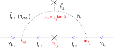
Figure 1: SUSY-Zee diagram

2 Zee Model in a Supersymmetric Framework

To take the Zee model seriously, one have to put it together with other aspects of beyond-standard-model physics. Hence it worths considering putting the model in a supersymmetric framework. The topic is studied in our recent paper[4], upon which the present report is based.

A naive idea along the line would be to add what is needed in the Zee mechanism to the minimal supersymmetric standard model (MSSM). However a right-handed slepton ($\tilde{\ell}_{\!\scriptscriptstyle R}$) actually has the same gauge quantum number as the Zee scalar boson, hence the question of our title — if the slepton could take the role. It is clear that, lepton number and, generically R-parity, has to be violated here. The MSSM spectrum even provides the second Higgs doublet needed. A careful study shows that all we need to complete the SUSY-Zee diagram is the following minimal set of only three R-parity violating (RPV) couplings:

$$\{\;\lambda_{{\scriptscriptstyle 12}\,k}\;,\;\lambda_{{\scriptscriptstyle 13}\,k}\;,\;\mu_{k}\;\}$$

where family index $k$ can be chosen arbitrarily with $\tilde{\ell}_{\!\scriptscriptstyle R_{k}}$ assuming the role of the Zee boson. The corresponding diagram is given in Fig.1. Note that our RPV parameters are defined in a flavor basis where the so-called sneutrino VEV’s are rotated away (see Refs.[5, 6] for more details).

It is interesting to note that the SUSY-Zee contribution to neutrino masses involves RPV parameters of both the bilinear and trilinear type. The existence of such a contribution under SUSY without R-parity has not been realized before our work. In fact, there is another contribution of the kind that exists even within the present minimal framework and, in that case, contributes to the same neutrino mass entries ($m_{e\mu}$ and $m_{e\tau}$) also first identified in Ref.[4]. This is shown in Fig.2.

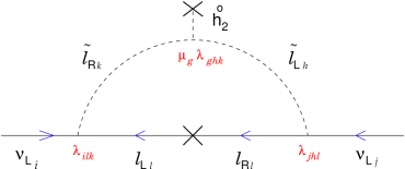
Figure 2: Another new contribution with both $\mu_{i}$ and $\lambda$’s

However, the above minimal set of RPV couplings also gives rise to other contributions that could potentially spoil the Zee mass texture. These more widely studied contributions tend to give diagonal mass matrix entries at least the same strength as the off-diagonal ones, as illustrated in Ref.[6]. To retain the successful flavor of the Zee model, one has to go to a region of the parameter space where the SUSY-Zee contribution dominates hence giving the zeroth order texture with the sub-dominating contributions fitting into a successful final result.

The best scenario here is for $k=3$, i.e. making the right-handed stau the Zee boson. We give here the neutrino mass results and summarize the required conditions as follows:

$$m_{ee}\! = \!\!\frac{-1}{16\pi^{2}}\;(A^{\!\scriptscriptstyle E}_{\tau}-\mu\tan\!\beta)\;f(M^{2}_{\tilde{\tau}_{L}},M^{2}_{\tilde{\tau}_{R}})\;m_{\tau}^{2}\,\lambda_{\scriptscriptstyle 1\!33}^{2}\;;$$ (3)

$$m_{\tau\tau}\! = \!\!\,\frac{-v^{2}\cos^{2}\!\beta\;(g^{2}M_{\scriptscriptstyle 1}+g^{{}^{\prime}2}M_{\scriptscriptstyle 2})}{2\mu\;[2\mu M_{\scriptscriptstyle 1}M_{\scriptscriptstyle 2}-v^{2}\sin\!\beta\cos\!\beta\;(g^{2}M_{\scriptscriptstyle 1}+g^{{}^{\prime}2}M_{\scriptscriptstyle 2})]}\;\mu_{\scriptscriptstyle 3}^{2}\;;$$ (4)

$$m_{e\mu}\! = \!\!\frac{-1}{16\pi^{2}}\frac{\sqrt{2}\tan\!\beta}{v\cos\!\beta}\;f(M_{h_{\scriptscriptstyle 1}^{\mbox{-}}}^{2},M_{\tilde{\tau}_{R}}^{2})\;m_{\tau}\,(m_{\mu}^{2}-m_{e}^{2})\,\mu_{\scriptscriptstyle 3}\lambda_{\scriptscriptstyle 1\!23}$$ (5)

$$-\frac{1}{16\pi^{2}}\frac{v\sin\!\beta}{\sqrt{2}}\;f(M_{\tilde{e}_{L}}^{2},M_{\tilde{\tau}_{R}}^{2})\;m_{\tau}\,\mu_{\scriptscriptstyle 3}\lambda_{\scriptscriptstyle 1\!23}\lambda_{\scriptscriptstyle 1\!33}^{2}\;;$$

$$m_{e\tau}\! = \!\!\frac{-1}{16\pi^{2}}\frac{\sqrt{2}\tan\!\beta}{v\cos\!\beta}\;f(M_{h_{\scriptscriptstyle 1}^{\mbox{-}}}^{2},M_{\tilde{\tau}_{R}}^{2})\;m_{\tau}\,(m_{\tau}^{2}-m_{e}^{2})\,\mu_{\scriptscriptstyle 3}\lambda_{\scriptscriptstyle 1\!33}$$ (6)

$$-\frac{1}{16\pi^{2}}\frac{v\sin\!\beta}{\sqrt{2}}\;f(M_{\tilde{e}_{L}}^{2},M_{\tilde{\tau}_{R}}^{2})\;m_{\tau}\,\mu_{\scriptscriptstyle 3}\lambda_{\scriptscriptstyle 1\!33}^{3}\;;$$

where $f(X,Y)=\frac{1}{X-Y}\;\log\frac{X}{Y}$; and with $m_{\mu\mu}$ and $m_{\mu\tau}$ being zero.

The conditions for the success of the scenario are given by :-

$$\lambda_{\scriptscriptstyle 1\!33} \sim \frac{m_{\mu}^{2}}{m_{\tau}^{2}}\;\lambda_{\scriptscriptstyle 1\!23}\;;$$ (7)

$$(\mu_{\scriptscriptstyle 3}\cos\!\beta)\;\lambda_{\scriptscriptstyle 1\!23} \sim \;{\cos^{3}\!\!\beta}\;{\mbox{Max}(M_{h_{\scriptscriptstyle 1}^{\mbox{-}}}^{2},M_{\tilde{\tau}_{R}}^{2})}\;(7\cdot 10^{-5}\,\mbox{GeV}^{-1})\;;$$ (8)

$${\mu_{\scriptscriptstyle 3}^{2}}\,\cos^{2}\!\!\beta \ll {\mu^{2}}M_{\scriptscriptstyle 1}\,(1\cdot 10^{-14}\,{\rm GeV}^{-1})\;;$$ (9)

$$\lambda_{\scriptscriptstyle 1\!33}^{2} \ll \frac{\mbox{Max}(M^{2}_{\tilde{\tau}_{L}},M^{2}_{\tilde{\tau}_{R}})}{(A^{\scriptscriptstyle E}_{\tau}-\mu\tan\!\beta)}\;(2.5\cdot 10^{-9}\,\mbox{GeV}^{-1})\;;$$ (10)

$$\frac{\lambda_{\scriptscriptstyle 1\!23}^{2}}{M^{2}_{\tilde{\tau}_{R}}} \leq 10^{-8}\,\mbox{GeV}^{-2}\;.$$ (11)

The feasibility of the scenario is marginal. Alternative versions with some extra chiral superfields, introduced and briefly discussed in Ref.[4], are much less contrained though.

References

- [1] A. Zee, Phys. Lett. 93B, 389 (1980).
- [2] P. Frampton and S. Glashow, Phys. Lett. B461, 95 (1999).
- [3] C. Jarlskog et.al., Phys. Lett. B449, 240 (1999).
- [4] K. Cheung and O.C.W. Kong, hep-ph/9912238, Phys. Rev. D61 (2000), (in press).
- [5] M. Bisset, O.C.W. Kong, C. Macesanu, and L. Orr, Phys. Lett. B430, 274 (1998); hep-ph/9811498, to be published in Phys. Rev. D (2000).
- [6] O.C.W. Kong, Mod. Phys. Lett. A14, 903 (1999).