OUTP-00-12P

hep-ph/0003207

March 2000

${}^{\prime\prime}+-+^{\prime\prime}$ Brane Model Phenomenology

Stavros Mouslopoulos and Antonios Papazoglou

Theoretical Physics, Department of Physics, Oxford University
1 Keble Road, Oxford, OX1 3NP, UK

Abstract

We explore the phenomenology of the recently proposed ${}^{\prime\prime}+-+^{\prime\prime}$ brane model which has a characteristic anomalously light first Kaluza-Klein mode. We consider the processes $e^{+}e^{-}\rightarrow\mu^{+}\mu^{-}$ and the Kaluza-Klein production $e^{+}e^{-}\rightarrow\gamma{\rm KK}$ giving missing visible energy. These in combination with the latest Cavendish experiments place severe bounds on the parameter space of the model. We also discuss how forthcoming experiments can test the model for “natural” range of the parameters.

1 Introduction

There has been a lot of interest during the past two years in models where the Standard Model (SM) fields are localized on a 3-brane in a higher dimensional spacetime . The motivation behind these constructions was the description and even solution of the long standing Planck hierarchy problem by geometrical means. The striking feature of these models is that they make dramatical phenomenological predictions which can be directly confronted with current and future collider experiments.

We can generally divide the recent brane-models into two classes. The first one pioneered by Antoniadis, Arkani-Hamed, Dimopoulos and Dvali [3], assumes factorizable geometry along the extra dimensions. The Planck hierarchy is then explained by the largeness of the compactification volume that suppresses the Planck scale and gives rise to a TeV fundamental mass scale ($M_{\rm Pl}^{2}=M^{n+2}V_{n}$). The size of the $n$ new dimensions can be as large as a millimeter without coming in conflict with experiment. The second class of models which were considered by Randall and Sundrum (RS) [4] assumes non-factorizable geometry (essentially spacetime is a slice of $AdS_{5}$) that associates each position on the extra dimension with different length scales, and thus different energy ones. The original RS construction consists of two parallel 3-branes of opposite tension sitting on the fixed points of an $S^{1}/Z_{2}$ orbifold. An exponential “warp” factor in the metric then generates a ratio of the mass scales between the two branes that could be $\mathcal{O}$$\left(10^{15}\right)$ although the size of the orbifold is of the order of Planck length. Assuming that the fundamental mass scale on the positive brane is of the order of $M_{\rm Pl}$ we can readily get a mass scale on the negative brane of the order the electroweak scale, thus solving the Planck hierarchy problem. In this model the compactification radius need only be some 35 times larger than the Planck length. However, living on a negative tension brane is generically problematic as far as cosmology is concerned unless we impose non-trivial constrains on the parameters of the model (see [5] for complete discussion).

In view of this difficulty Kogan, Mouslopoulos, Papazoglou, Ross and Santiago [6] proposed a brane configuration with two ${}^{\prime\prime}+^{\prime\prime}$ branes sitting on the fixed points of an $S^{1}/Z_{2}$ orbifold and an intermediate ${}^{\prime\prime}-^{\prime\prime}$ brane (see Fig. 1). In this ${}^{\prime\prime}+-+^{\prime\prime}$ model our universe is the third ${}^{\prime\prime}+^{\prime\prime}$ brane and a desired hierarchy can be generated by adjusting the size of the orbifold and the position of the intermediate ${}^{\prime\prime}-^{\prime\prime}$ brane. The above contruction appears to be special because the equivalent quantum mechanical problem, that arises from the Einstein equations after some coordinate and field redefinitions, has a double “volcano” form and supports in addition to the bound state graviton zero mode, an anomalously light and strongly coupled first KK mode “bound” state. In Ref. [6] we presented a preliminary study of the $e^{+}e^{-}\rightarrow\mu^{+}\mu^{-}$ cross section for a specific value of the $w$ and $k$ parameters (see section 2 for definitions) paying particular regard to the characteristic behaviour of the first KK mode.

It is worth mentioning that in the context of [6] if one drops the requirement of solving the hierarchy problem, one finds the exotic possibility of “bigravity”. In this case, gravitational attraction is a result of the exchange of ordinary 4D graviton plus an ultralight first KK state with Compton wavelength which might be $1\%$ of the size of the observable universe, thus generating modifications of gravity not only at small but also at ultra-large distances. The latter characteristic was also found in a brane construction by Gregory, Rubakov and Sibiryakov [7], which was recently shown to be closely related to the ${}^{\prime\prime}+-+^{\prime\prime}$ model (see [8]). However, as it is widely known [14] the modulus corresponding to the moving negative tension brane in both cases is a physical ghost, something very unattractive for these models. Nevertheless, as proposed by [15] the stabilization mechanism might offer a way out of this problem.

Figure 1: ${}^{\prime\prime}+-+^{\prime\prime}$ model with two ${}^{\prime\prime}+^{\prime\prime}$ branes at the fixed points of a $S^{1}/Z_{2}$ orbifold and a ${}^{\prime\prime}-^{\prime\prime}$ brane in between.

In the present paper we will not discuss the “bigravity” possibility, but concentrate on the case that the ${}^{\prime\prime}+-+^{\prime\prime}$ model can offer a resolution to the Planck hierarchy problem. Our aim is to further develop its collider phenomenology for different values of the $w$ and $k$ parameters and to include the constraints from missing energy processes. The region of the parameter space that can be considered as “natural”, in the sense that they solve the hierarchy problem, is examined in detail. It turns out that different parts of the parameter space are sensitive to different type of processes, thus giving us a clear picture of the expected signatures of the model.

The organization of the paper is as follows. In the next Section we review the main characteristics of the ${}^{\prime\prime}+-+^{\prime\prime}$ model. In Section 3 we discuss the phenomenology of the $e^{+}e^{-}\rightarrow\mu^{+}\mu^{-}$ and the $e^{+}e^{-}\rightarrow\gamma{\rm KK}$ processes for different values of the warp factor $w$ and $k$. Finally, we present our conclusions.

2 Characteristics of the ${}^{\prime\prime}+-+^{\prime\prime}$ model

The ${}^{\prime\prime}+-+^{\prime\prime}$ model presented in [6] (see Fig. 1) has as a starting point the action:

$$S=\int d^{4}x\int_{-L_{2}}^{L_{2}}dy\sqrt{-G}\{-\Lambda+2M^{3}R\}-\sum_{i}\int_{y=L_{i}}d^{4}xV_{i}\sqrt{-\hat{G}^{(i)}}$$ (1)

where $M$ is the 5-D fundamental scale, $\Lambda$ is the bulk cosmological constant, $\hat{G}^{(i)}_{\mu\nu}$ is the induced metric on the branes and $V_{i}$ their tensions. The ${}^{\prime\prime}+^{\prime\prime}$ branes are situated at the fixed points $L_{0}=0$, $L_{2}$ and the ${}^{\prime\prime}-^{\prime\prime}$ brane at $L_{1}$.

Taking the metric ansatz that respects 4D Poincaré invariance to be :

$$ds^{2}=e^{-2\sigma(y)}\eta_{\mu\nu}dx^{\mu}dx^{\nu}+dy^{2}$$ (2)

the Einstein equations give a solution for the $\sigma(y)$ function:

$$\sigma(y)=k\left\{L_{1}-\left||y|-L_{1}\right|\right\}$$ (3)

with the requirement that the brane tensions are tuned to $V_{0}=-\Lambda/k>0$, $V_{1}=\Lambda/k<0$, $V_{2}=-\Lambda/k>0$. The parameter $k$ is a measure of the curvature of the bulk and is given by $k=\sqrt{\frac{-\Lambda}{24M^{3}}}$. The 4D Planck mass, the fundamental scale $M$ and the parameter $k$ are related by the equation:

$$M_{\rm Pl}^{2}=\frac{M^{3}}{k}\left[1-2e^{-2kL_{1}}+e^{-2k(2L_{1}-L2)}\right]$$ (4)

It is obvious that for large enough $kL_{1}$ and $k\left(2L_{1}-L_{2}\right)$ the three mass scales $M_{\rm Pl}$, $M$, $k$ can be taken to be of the same order. The “warp” factor responsible for the generation of the desired hierarchy on the third brane is simply:

$$w=e^{-\sigma\left(L_{2}\right)}=e^{-k\left(2L_{1}-L_{2}\right)}$$ (5)

The KK spectrum is determined by considering the (linear) fluctuations of the metric ansatz. It turns out that there is always a zero mode that corresponds to the ordinary 4-D graviton. The KK masses are determined by the the quantization determinant:

$$\left|\begin{array}[]{cccc}J_{1}\left(\frac{m}{k}\right)&Y_{1}\left(\frac{m}{k}\right)&\phantom{-}0&\phantom{-}0\\ 0&0&\phantom{-}J_{1}\left(\frac{m}{k}e^{k(2L_{1}-L_{2})}\right)&\phantom{-}Y_{1}\left(\frac{m}{k}e^{k(2L_{1}-L_{2})}\right)\\ J_{1}\left(\frac{m}{k}e^{kL_{1}}\right)&Y_{1}\left(\frac{m}{k}e^{kL_{1}}\right)&\phantom{-}J_{1}\left(\frac{m}{k}e^{kL_{1}}\right)&\phantom{-}Y_{1}\left(\frac{m}{k}e^{kL_{1}}\right)\\ J_{2}\left(\frac{m}{k}e^{kL_{1}}\right)&Y_{2}\left(\frac{m}{k}e^{kL_{1}}\right)&-J_{2}\left(\frac{m}{k}e^{kL_{1}}\right)&-Y_{2}\left(\frac{m}{k}e^{kL_{1}}\right)\end{array}\right|=0$$ (6)

(where we have suppressed the subscript $n$ on the masses $m_{n}$)

Denoting the separation between the last two branes by $x=k(L_{2}-L_{1})$ we calculate the mass of the first KK state:

$$m_{1}=2kwe^{-2x}$$ (7)

Numerically, we find that the masses of the remaining KK states depend in a different way on the parameter $x$. The masses of the second state and the spacing $\Delta m$ between the subsequent states have the form:

$$m_{2} \approx 4kwe^{-x}$$ (8)

$$\Delta m \approx \varepsilon kwe^{-x}$$ (9)

with $\varepsilon$ a number between 1 and 2. The spacing only approaches a constant for high enough levels when the arguments of the Bessel functions become much greater than one.

The interaction of the KK states to the SM particles is found as in Ref. [6] to be:

$${\mathcal{L}}_{int}=-\frac{1}{M_{\rm Pl}}h_{\mu\nu}^{(0)}(x)T_{\mu\nu}\left(x\right)-\sum_{n>0}\frac{1}{c_{n}}h_{\mu\nu}^{(n)}(x)T_{\mu\nu}\left(x\right)$$ (10)

where $T_{\mu\nu}$ is the stress energy momentum tensor of the SM Lagrangian, $h_{\mu\nu}^{(0)}(x)$ the 4-D graviton, $h_{\mu\nu}^{(n)}(x)$ the $n$th level KK state and $c_{n}$ the corresponding coupling suppressions of them.

The coupling suppression of the first KK mode is independent of $x$ and equal to

$$c_{1}=wM_{\rm Pl}$$ (11)

while the coupling suppressions of the higher modes are enhanced relative to the lowest mode by a factor proportional to $e^{x}$.

The above masses and coupling suppressions have been computed in the region of large $x$ were the Bessel functions can be approximated by the first terms of their power series (note that since the parameter $x$ appears in exponentials we actually have very good approximations for $x\mathrel{\raise 1.29167pt\hbox{$>$\kern-7.5pt\lower 4.30554pt\hbox{$\sim$}}}3$). However for lower $x$’s the above approximations break down and the first mode is not so different from the other KK states. In the extreme case where the positions of the second and the third brane coincide, the positive brane disappears and we obtain the original RS model. The phenomenology of the latter has been extensively studied in [9].

3 Phenomenology

In this Section we will present a discussion of the phenomenology of the KK modes to be expected in high energy colliders, concentrating on the simple and sensitive to new physics processes $e^{+}e^{-}\rightarrow\mu^{+}\mu^{-}$ (this analysis is readily generalized to include $q\bar{q}$, $gg$ initial and final states) and $e^{+}e^{-}\rightarrow\gamma+\mbox{{missing energy}}$. Since the characteristics of the phenomenology depend on the parameters of the model ($w$,$k$,$x$) we explore the regions of the parameter space that are of special interest (i.e. give hierarchy factor $\mathcal{O}$$\left(10^{15}\right)$ and do not introduce a new hierarchy between $k$ and $M$ as seen from equation (4)).

3.1 $e^{+}e^{-}\rightarrow\mu^{+}\mu^{-}$ process

Figure 2: $e^{+}e^{-}\rightarrow\mu^{+}\mu^{-}$

Using the Feynman rules of Ref. [11] the contribution of the KK modes to $e^{+}e^{-}\rightarrow\mu^{+}\mu^{-}$ is given by

$$\sigma\left(e^{+}e^{-}\rightarrow\mu^{+}\mu^{-}\right)=\frac{s^{3}}{1280\pi}|D(s)|^{2}$$ (12)

where $D(s)$ is the sum over the propagators multiplied by the appropriate coupling suppressions:

$$D(s)=\sum_{n>0}\frac{1/c_{n}^{2}}{s-m_{n}^{2}+i\Gamma_{n}m_{n}}$$ (13)

and $s$ is the center of mass energy of $e^{+}e^{-}$.

Note that the bad high energy behaviour (a violation of perturbative unitarity) of this cross section is expected since we are working with an effective - low energy non-renormalizable theory of gravity. We assume our effective theory is valid up to an energy scale $M_{s}$ (which is ${\mathcal{O}}({\rm TeV})$), which acts as an ultraviolet cutoff. The theory that applies above this scale is supposed to give a consistent description of quantum gravity. Since this is unknown we are only able to determine the contributions of the KK states with masses less than this scale. This means that the summation in the previous formula should stop at the KK mode with mass near the cutoff.

For the details of the calculation it will be important to know the decay rates of the KK states. These are given by:

$$\Gamma_{n}=\beta\frac{m_{n}^{3}}{c_{n}^{2}}$$ (14)

where $\beta$ is a dimensionless constant that is between $\frac{39}{320\pi}\approx 0.039$ (in the case that the KK is light enough, i.e. smaller than $0.5{\rm MeV}$, so that it decays only to massless gauge bosons and neutrinos) and $\frac{71}{240\pi}\approx 0.094$ (in the case where the KK is heavy enough that can decay to all SM particles).

If we consider $w$ and $k$ fixed, then when $x$ is smaller than a certain value $x_{0}=x_{0}(w,k)$ we have a widely spaced discrete spectrum (from the point of view of TeV physics) close to the one of the RS case with cross section at a KK resonances of the form $\sigma_{res}\sim s^{3}/m_{n}^{8}$ (see [9]). For the discrete spectrum there is always a range of values of the $x$ parameter so that the KK resonances are in the range of energies of collider experiments. In these cases we calculate the excess over the SM contribution which would have been seen either by direct scanning if the resonance is near the energy at which the experiments actually run or by means of the process $e^{+}e^{-}\rightarrow\gamma\mu^{+}\mu^{-}$ which scans a continuum of energies below the center of mass energy of the experiment (of course if $k$ is raised the KK modes become heavier and there will be a value for which the lightest KK mode is above the experimental limits).

For values of $x$ greater than $x_{0}(k,w)$ the spacing in the spectrum is so small that we can safely consider it to be continuous. At this point we have to note that we consider that the “continuum” starts at the point where the convoluted KK resonances start to overlap. In this case we substitute in $D(s)$ the sum for $n\geq 2$ by an integral over the mass of the KK excitations, i.e.

$$D(s)_{KK}\approx\frac{1/c_{1}^{2}}{s-m_{1}^{2}+i\Gamma_{1}m_{1}}+\frac{1}{\Delta m\;c^{2}}\int_{m_{2}}^{M_{s}}dm\;\frac{1}{s-m^{2}+i\epsilon}$$ (15)

where the value of the integral is $\sim i\pi/2\sqrt{s}$ with the principal value negligible in the region of interest ($\sqrt{s}\ll M_{s}$) and we have considered constant coupling suppression $c$ for the modes with $n\geq 2$ (approximation that turns out to be reasonable as the coupling saturates quickly as we consider higher and higher levels). The first state is singled out because of its different coupling.

3.2 $e^{+}e^{-}\rightarrow\gamma+\mbox{{missing energy}}$ process

The missing energy processes in the SM (i.e. $e^{+}e^{-}\rightarrow\gamma\nu\bar{\nu}$) are well explored and are a standard way to count the number of neutrino species. In the presence of the KK modes there is also a possibility that any KK mode produced, if it has large enough lifetime, escapes from the detector before decaying, thus giving us an additional missing energy signal. The new diagrams that contribute to this effect are the ones in the Fig. 3.

Figure 3: $e^{+}e^{-}\rightarrow\gamma$ KK

The differential cross section of the production of a KK mode plus a photon is given by Ref. [12] and is equal to:

$$\frac{d\sigma}{dt}(e^{+}e^{-}\rightarrow\gamma+{\rm{KK}})=\frac{\alpha}{16}\sum_{n>0}\frac{1}{c_{n}^{2}s}F\left(\frac{t}{s},\frac{m_{n}^{2}}{s}\right)$$ (16)

where $s$, $t$ are the usual Mandelstam variables and the function $F$ is given by:

$$F(x,y)=\frac{1}{x(y-1-x)}[ -4x(1-x)(1+2x+2x^{2})+y(1+6x+18x^{2}+16x^{3})$$ (17)

$$-6y^{2}x(1+2x)+y^{3}(1+4x)\phantom{0}]$$

A reasonable size of a detector is of the order of $d=1$m, so we assume that the events of KK production are counted as missing energy ones if the KK modes survive at least for distance d from the interaction point (this excludes decays in neutrino pairs which always give missing energy signal). We can then find a limit on the KK masses that contribute to the experimental measurement. By a straightforward relativistic calculation we find that this is the case if:

$$\Gamma_{n}<\frac{E_{\gamma}}{m_{n}d}=\frac{s-m_{n}^{2}}{2\sqrt{s}m_{n}d}$$ (18)

From equation 14 we see that this can be done if:

$$m_{n}<\sqrt{\frac{-c_{n}^{2}+c_{n}\sqrt{c_{n}^{2}+8\beta ds^{3/2}}}{4\beta d\sqrt{s}}}$$ (19)

It turns out that usually only the first KK state mass satisfies this condition and decays outside the detector. All the other states have such short lifetimes that decay inside the detector and so are not counted as missing energy events (again this excludes decays in neutrino pairs). In the regions of the parameter space where this was not the case, we found that only a very small part of the KK tower contributed and didn’t give any important excess in comparison with the one from the first state alone. Thus, taking only the contribution of the first KK state and imposing the kinematic cuts given by the experiments on the angular integration, we found the measurable cross section. This cross section has to be compared to the error of the experimentally measured cross section because so far the SM predictions coincide with the measured value.

The most stringent measurement available is the one by OPAL Collaboration [13] at $\sqrt{s}=183$GeV. The measured cross section is $\sigma_{meas}=4.71\pm 0.34$pb so the values of the parameters of the model that give cross section greater than $0.34$pb are excluded. Since the main contribution comes from the first KK state and because its coupling depends only on the warp factor $w$, we will either exclude or allow the whole k-x plane for a given $w$. The critical value of $w$ that the KK production cross section equals to the experimental error is $w=1.8e^{-35}$.

It is worth noting that the above cross section is almost constant for different center of mass energies $\sqrt{s}$, so ongoing experiments with smaller errors (provided that they are in accordance with the SM prediction) will push the bound on $w$ further ahead.

3.3 Cavendish experiments

A further bound on the parameters of our model can be put from the Cavendish experiments. The fact that gravity is Newtonian at least down to millimeter distances implies that the corrections to gravitational law due to the presence of the KK states must be negligible for such distances. The gravitational potential is the Newton law plus a Yukawa potential due to the exchange of the KK massive particles (in the Newtonian limit):

$$V(r)=-\frac{1}{M_{\rm Pl}^{2}}\frac{M_{1}M_{2}}{r}\left(1+\sum_{n>0}\left(\frac{M_{\rm Pl}}{c_{n}}\right)^{2}e^{-m_{n}r}\right)$$ (20)

The contribution to the above sum of the second and higher modes is negligible compared with the one of the first KK state, because they have larger masses and coupling suppressions. Thus, the condition for the corrections of the Newton law to be small for millimeter scale distances is:

$$x<\tilde{x}=15-\frac{1}{2}{\rm ln}\left(\frac{-{\rm ln}w}{kw}{\rm GeV}\right)$$ (21)

3.4 $k-x$ plots

As mentioned above the range of the parameter space that we explore is chosen so that it corresponds to the region of physical interest giving rise to the observed hierarchy between the electroweak and the Planck scale i.e. $w\sim 10^{-15}$, $k\sim M_{\rm Pl}$. The allowed regions (unshaded areas) for $w=4.5e^{-35}$ and $w=10e^{-35}$ are shown in the Figures  5 and  5. The bounds from the previously mentioned experiments and the form of the diagram will be now explained in detail.

• $e^{+}e^{-}\rightarrow\mu^{+}\mu^{-}$ bounds

As we noted in section 3.1, for relatively small values of $x$ the spectrum is discrete and as $x$ increases it tends to a continuum (the dashed line shows approximately where we the spectrum turns from discrete to continuum). In case of the continuum, for the parameter region that we explore, it turns out that it does not give any bound since the excess over the SM cross section becomes important only for energies much larger than $200$GeV. However there are significant bounds coming from the discrete spectrum region, since generally we have KK resonances in the experimentally accessible region and the convolution of some of them will give significant excess to the SM background. The exclusion region coming from $e^{+}e^{-}\rightarrow\mu^{+}\mu^{-}$, is the region between the curves (1) and (2). The details of the bound depend on the behaviour of the couplings and the masses. In this case the bounds start when the KK states have sufficiently large width and height (i.e. large mass and coupling). This is the reason why curve (2) bends to the left as k increases. The shape of the upper part of the curve (2) comes from the fact that by increasing $k$ we push the masses of the KK states to larger values so that there is the possibility that the first KK state has mass smaller that $20$GeV and at the same time the rest of tower is above $200$GeV (the dotted line is where the second KK states is at $200$GeV). The last region is not experimentally explored at present. An increase of $w$ decreases all the couplings and thus this will push the bound even more to the left. Decreasing $w$ (e.g. $w=e^{-35}$), on the contrary will increase the values of the couplings and there are strict bounds coming both from the discrete and the continuum. The $e^{+}e^{-}\rightarrow\mu^{+}\mu^{-}$ experiments don’t give any bound when the first KK state has mass bigger than $\sim 200$GeV, since in this case the KK resonances cannot be produced from current experiments and the low energy effects are negligible for the range of parameters that we examine (this region is represented by the triangle at the upper left corner of the plot). As colliders probe higher center of mass energies the curve (1) will be pushed to the left and curve (2) to the right.

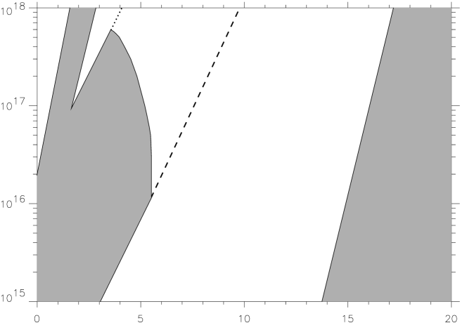
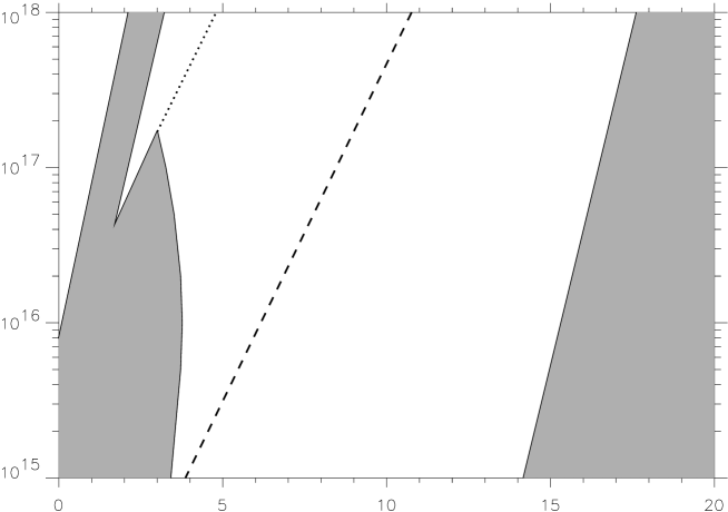
Figure 4: Excluded regions (shaded areas) for $w=4.5e^{-35}$.

Figure 5: Excluded regions (shaded areas) for $w=10e^{-35}$.

• Missing energy bounds

As we noted in section 3.2, the KK states have generally very short lifetime. For certain value of $w$, the main contribution to the cross section comes from the first KK state, since the restriction on the mass (so that the KK states escape the detector) means that only a few states contribute, even near the boundary of Cavendish bounds where the spacing of the tower is very small. Decreasing the value of $w$, we increase the coupling of the first KK state so for the values of $w<1.8e^{-35}$ the contribution from the first KK state becomes so big that excludes all the region between $e^{+}e^{-}\rightarrow\mu^{+}\mu^{-}$ and the Cavendish bound (the region with the KK tower over $200$GeV always survives). Variation of the $k$, $x$ parameters in this case does not change significantly the cross section, because the main contribution comes from the first KK mode whose coupling is constant i.e. independent of $k$, $x$ and since although its mass, $m_{1}$ depends on $k$ the cross section is insensitive to the mass changes because it is evaluated at energy $\sqrt{s}=183$GeV where the cross section has saturated. To summarize, the missing energy bounds either exclude the whole region between the $e^{+}e^{-}\rightarrow\mu^{+}\mu^{-}$ and the Cavendish limits or nothing at all (due to the smallness of the coupling). Additionally, the missing energy experiments don’t give any bound when the first KK state has mass bigger than $\sim 143$GeV, since in this case the emitted photon has energy smaller than the experimental cuts. Currently running and forthcoming colliders will push the bound of $w$ to larger values.

• Cavendish bounds

From the discussion in section 3.3 we see that the bound on the parameter space from Cavendish experiments comes from Eq. (21). The exclusion region is the one that extends to the right of the line (3) of the plots. For fixed $k$, $w$ the Cavendish bounds exclude the region $x>\tilde{x}(k,w)$ due to the fact that the first KK becomes very light (and its coupling remains constant). Now if we increase $k$, since the masses of the KK are proportional to it, we will have an exclusion region of $x>\tilde{x}(k^{\prime},w)$, with $\tilde{x}(k^{\prime},w)>\tilde{x}(k,w)$. This explains the form of the Cavendish bounds. When we increase the $w$ parameter the whole bound will move to the right since the couplings of the KK states decrease. Future Cavendish experiments testing the Newton’s law at smaller distances will push the curve (3) to the left.

4 Conclusions

In this paper we discussed the phenomenology of the ${}^{\prime\prime}+-+^{\prime\prime}$ model, presented in [6]. This was done by considering processes sensitive to the new physics, namely the $e^{+}e^{-}\rightarrow\mu^{+}\mu^{-}$ and the $e^{+}e^{-}\rightarrow\gamma{\rm KK}$. We examined the parameter space that is of physical interest (i.e. creates the hierarchy between the $M_{\rm Pl}$ and $M_{\rm E/W}$). Different regions of the parameter space are sensitive to different experiments. The previous experiments in combination with the latest Cavendish experiments place bounds on the parameter space of the model, as shown in Figs. 5 and 5. As it can be seen there is still a lot of the parameter space that is not presently excluded.

Acknowledgments: We are grateful to our supervisors Ian I. Kogan and Graham G. Ross for useful discussions and comments and to Peter B. Renton for providing us the LEP beam spreads. S.M.’s work is supported by the Hellenic State Scholarship Foundation (IKY) No. 8117781027. A.P.’s work is supported by the Hellenic State Scholarship Foundation (IKY) No. 8017711802.

References

- [1]
-
[2]
K. Akama in Gauge Theory and Gravitation, Proceedings
of the International Symposium, Nara, Japan, 1982,
ed. K.Kikkawa, N.Nakanishi and H. Nariai
(Springer-Verlag, 1983), 267;
e-version is: K.Akama, hep-th/0001113;
V.A.Rubakov and M.E. Shaposhnikov, Phys. Lett. B125 (1983) 136;
M. Visser, Phys. Lett. B159 (1985) 22;
E. J. Squires, Phys. Lett. B167 (1985) 286. -
[3]
N. Arkani-Hamed, S. Dimopoulos and G. Dvali,
Phys. Lett. B429 (1998) 263;
N. Arkani-Hamed, S. Dimopoulos and G. Dvali, Phys. Rev. D59 (1999) 086004;
I. Antoniadis, N. Arkani-Hamed, S. Dimopoulos and G. Dvali, Phys. Lett. B436 (1998) 257. -
[4]
L. Randall and R. Sundrum, Phys. Rev. Lett. 83 (1999)
3370;
L. Randall and R. Sundrum, Phys. Rev. Lett. 83 (1999) 4690. -
[5]
A. Lukas, B.A. Ovrut, K.S. Stelle and D. Waldram,
Phys. Rev. D59 (1999) 086001;
A. Lukas, B.A. Ovrut and D. Waldram, Phys. Rev. D60 (1999) 086001;
N. Kaloper and A. Linde, Phys. Rev. D59 (1999) 101303;
P. Binétruy, C. Deffayet and D. Langlois, hep-th/9905012;
T. Nihei, Phys. Lett. B465 (1999) 81;
N. Kaloper, Phys. Rev. D60 (1999) 123506;
C. Csáki, M. Graesser, C. Kolda and J. Terning, Phys. Lett. B462 (1999) 34;
J.M. Cline, C. Grojean and G. Servant, Phys. Rev. Lett. 83 (1999) 4245;
H.B. Kim and H.D. Kim, Phys. Rev. D61 (2000) 064003;
H.B. Kim, hep-th/0001209;
P. Kanti, I.I. Kogan, K.A. Olive and M. Pospelov, Phys. Lett. B468 (1999) 31;
P. Kanti, I.I. Kogan, K.A. Olive and M. Pospelov, hep- ph/9912266;
P. Kanti, K.A. Olive and M. Pospelov, hep- ph/0002229. - [6] I.I. Kogan, S. Mouslopoulos, A. Papazoglou, G.G. Ross and J. Santiago, hep-ph/9912552.
- [7] R. Gregory, V.A. Rubakov and S.M. Sibiryakov, hep-th/0002072.
- [8] I.I. Kogan and G.G.Ross, hep-th/0003074.
-
[9]
H. Davoudiasl, J.L. Hewett and T.G. Rizzo, hep-ph/9909255;
S. Chang and M. Yamaguchi, hep-ph/9909523. -
[10]
W.D. Goldberger and M.B. Wise, Phys. Rev. D60 (1999)
107505;
W.D. Goldberger and M.B. Wise, Phys. Rev. Lett. 83 (1999) 4922;
W.D. Goldberger and M.B. Wise, hep-ph/9911457;
O. De Wolfe, D.Z. Freedman, S.S. Gubser and A. Karch, hep-th/9909134;
M.A. Luty and R. Sundrum, hep-th/9910202;
C. Csáki, M. Graesser, L. Randall, and J. Terning, hep-ph/9911406;
C. Charmousis, R. Gregory and V.A. Rubakov, hep-th/9912160;
T. Tanaka and X. Montes, hep-th/0001092;
S.B. Bae, P. Ko and H.S. Lee, hep-ph/0002224;
U. Mahanta and S. Rakshit, Phys.Lett. B480 (2000) 176;
U. Mahanta and A. Datta, hep-ph/0002183. - [11] T. Han, J.D. Lykken and R.J. Zhang, Phys. Rev. D59 (1999) 105006.
- [12] G.F. Giudice, R. Rattazzi and J.D. Wells, Nucl. Phys. B544 (1999) 3.
- [13] The OPAL Collaboration, Eur. Phys. J. C8 (1999) 23.
- [14] L. Pilo, R. Rattazzi and A. Zaffaroni, hep-th/0004028.
- [15] I.I. Kogan, S. Mouslopoulos, A. Papazoglou and G.G. Ross, hep-th/0006030.