Quantum fluctuations of the quark condensate.

Abstract

The quantum fluctuations of the quark condensate are studied in a Nambu Jona-Lasinio model. Two Lorenz invariant regularizations are considered: a sharp 4-momentum cut-off and a soft gaussian regulator. The quantum fluctuations of the quark condensate are found to be large although chiral symmetry is not restored. Instabilities of the ground state appear when the system is probed by a source term proportional to the squared quark condensate. The instabilities are traced to unphysical poles introduced by the regulator and their effect is greatly enhanced when a sharp cut-off is used.

1 Introduction.

We study the effect of quantum fluctuations of the quark condensate on the physical vacuum. We use an $SU\left(2\right)_{f}$ Nambu Jona-Lasinio model in the chiral limit. Two ultra-violet regularizations are considered:

• regularization using a sharp cut-off, in which the quark propagators are set to zero when $k_{\mu}^{2}>\Lambda^{2}$, where $k_{\mu}$ is the euclidean 4-momentum of the quark propagator;

• regularization using a smooth gaussian regulator which will be described below.

We introduce a current quark mass $m$ as a source term $m\bar{\psi}\psi$ to calculate the quark condensate $\left\langle\bar{\psi}\psi\right\rangle$. We introduce another source term $\frac{1}{2}j\left(\bar{\psi}\Gamma_{a}\psi\right)^{2}$ which allows us to calculate the expectation value $\left\langle\left(\bar{\psi}\Gamma_{a}\psi\right)^{2}\right\rangle$ of the squared quark condensate. We shall however maintain $j$ at a finite value in order to study the response of the system to a deformation induced by this source term. We include the $1/N_{c}$ effects due to the quantum fluctuations of the meson fields. In the quark language, this means that we include the exchange (Fock) term as well as the (RPA) ring diagrams.

Although the quantum fluctuations of the meson fields do not restore chiral symmetry, we do find surprisingly large fluctuations of the quark condensate. We also find that the effective potential is very sensitive to the shape of the regulator. Apparent instabilities appear which we show to be artefacts sharp cut-of used in conjunction with the relatively low values of the cut-offs, used in chiral quark models.

The quantum fluctuations of the meson fields in the Nambu Jona-Lasinio model have been studied for several years [1], [2], [3], [4]. In these studies, the quark and meson loops were regularized with different cut-offs. Since both the quark and meson loops diverge, their relative contribution could be adjusted at will by a proper choice of the cut-offs thereby making it impossible to estimate the importance of the quantum fluctuations of the meson fields.

In this study we consider the Nambu Jona-Lasinio model to be a quark model in the sense that all physical processes can be expressed in term of Feynman graphs involving only quark propagators. The meson fields which are introduced in the process of bosonization are mere intermediate quantities introduced to calculate the partition function. When the quark propagators are regularized, a single cut-off regularizes both the quark and meson loops. No further regularization is required for higher order loops. This approach has also been adopted in Ref.[5] for example, with the exception that a 3-momentum cut-off was used. We shall show that results obtained with 3 and 4-momentum cut-offs can differ even qualitatively. We show that regularization with a 4-momentum cut-off introduces a non-locality which makes the ground state energy unbounded from below, or, equivalently, which makes the model acausal. We relate this instability to the unphysical poles of the quark propagator which are introduced by the regulator.

We consider the regularization of a model to be a physical phenomenon and not simply a way to be rid of infinities wherever they turn up. Because of this we regularize the model action from the outset before calculating the loop integrals and we shall see that this makes a significant difference with the common practice of regularizing the infinities of the loop integrals which are deduced from an unregularized action. We derive all quantities in terms of a regulator which is a function of the squared euclidean 4-momentum $k^{2}$.

The paper is composed of three parts. In the first part we set the notation, we explain how the calculation was performed and we define the relevant range of the model parameters. The second part is devoted to a discussion of the quantum fluctuations of the quark condensate. The last part discusses the instabilities which are displayed by the response of the system, subject to constraint proportional to the squared quark condensate.

2 The model euclidean action.

The model is defined by the euclidean action:

$$I_{m}\left(q,\bar{q}\right)=\left\langle\bar{q}\left|-i\partial_{\mu}\gamma_{\mu}+rmr\right|q\right\rangle-\frac{g^{2}}{2N_{c}}\int d_{4}x\left(\left\langle\bar{q}\left|r\right|x\right\rangle\Gamma_{a}\left\langle x\left|r\right|q\right\rangle\right)^{2}$$ (1)

It involves a quark field $q\left(x\right)\equiv\left\langle x\left|q\right.\right\rangle$. The euclidean Dirac matrices are $\gamma_{\mu}=\gamma^{\mu}=\left(i\beta,\vec{\gamma}\right)$. The model includes a regulator $r$ which is assumed to be diagonal in $k$-space: $\left\langle k\left|r\right|k^{\prime}\right\rangle=\delta_{kk^{\prime}}r\left(k\right)$. We consider both a gaussian regulator:

$$r\left(k\right)=e^{-\frac{k^{2}}{2\Lambda^{2}}}$$ (2)

and a sharp cut-off:

$$r\left(k\right)=1\;\;if\;\;k^{2}<\Lambda^{2}\quad\quad\quad r\left(k\right)=0\;\;if\;\;k^{2}>\Lambda^{2}$$ (3)

The use of the the sharp cut-off is tantamount to the calculation of Feynman graphs in which the quark propagators are set to zero when their euclidean 4-momentum $k_{\mu}^{2}$ exceeds the cut-off $\Lambda^{2}$. The bra-ket notation for the Dirac fields is:

$$\left\langle\bar{q}\left|-i\partial_{\mu}\gamma_{\mu}+m\right|q\right\rangle\equiv\int d_{4}x\,\bar{q}\left(x\right)\left(-i\partial_{\mu}\gamma_{\mu}+m\right)q\left(x\right)$$

$$\left\langle x\left|r\right|q\right\rangle=\int d_{4}y\,\left\langle x\left|r\right|y\right\rangle\,q\left(y\right)\quad\quad\left\langle\bar{q}\left|r\right|x\right\rangle=\int d_{4}y\,\,\bar{q}\left(y\right)\,\left\langle y\left|r\right|x\right\rangle\quad\quad$$ (4)

We use the current quark mass $m$ to evaluate a regularized quark condensate and that is why the current quark mass $m$ is multiplied by the regulator. The $\Gamma_{a}=\left(1,i\gamma_{5}\vec{\tau}\right)$ are the generators of chiral rotations. The number of flavors is $N_{f}$ and there are $N_{f}^{2}$ generators $\Gamma_{a}$. We assumed that the coupling constant $\frac{g^{2}}{N_{c}}$ is inversely proportional to $N_{c}$.

The partition function $W$ is given by the euclidean path integral:

$$e^{-W\left(m\right)}=\int D\left(q\right)D\left(\bar{q}\right)e^{-I\left(q,\bar{q}\right)}$$ (5)

At zero temperature and for an infinite translationally invariant system, $W=\Omega\varepsilon$ where $\Omega$ is the space-time volume $\Omega=\int d_{4}x\,1$ and where $\varepsilon$ is the energy density $\varepsilon=\frac{E}{V}$, which is the energy per unit volume of the system in its ground state.

The model is regularized in the same way as the effective quark model which has been derived from a study of the propagation of quarks in an instanton liquid [6],[7] in which case both the shape of the regulator and the value of the cut-off are derived. However, the model action (1) we are using is not exactly the same as that derived from the instanton liquid [8]. The model described by the action (1) has been actively investigated in both the soliton [9] and meson sectors [10] [11, 12].

We now adopt a notation which adds considerable transparency to the manipulations made below. We define an interaction $V$ by its matrix element:

$$\left\langle xa\left|V\right|yb\right\rangle=\left\langle yb\left|V\right|xq\right\rangle=-\delta_{ab}\delta\left(x-y\right)\frac{g^{2}}{N_{c}}\quad\quad\quad\left\langle xa\left|V^{-1}\right|yb\right\rangle=-\delta_{ab}\delta\left(x-y\right)\frac{N_{c}}{g^{2}}$$ (6)

We define a delocalized quark field $\psi\left(x\right)$ and the corresponding bilinear forms $\bar{\psi}\Gamma_{a}\psi$:

$$\psi\left(x\right)=\int d_{4}x\,\left\langle x\left|r\right|y\right\rangle\,q\left(y\right)\quad\quad\quad\bar{\psi}\left(x\right)\Gamma_{a}\psi\left(x\right)=\int d_{4}y\,d_{4}z\,\bar{q}\left(y\right)\left\langle y\left|r\right|x\right\rangle\Gamma_{a}\left\langle x\left|r\right|z\right\rangle q\left(z\right)$$ (7)

In this notation, the action (1) takes the form:

$$I_{m}\left(q,\bar{q}\right)=\left\langle\bar{q}\left|-i\partial_{\mu}\gamma_{\mu}+rmr\right|q\right\rangle+\frac{1}{2}\left(\bar{\psi}\Gamma\psi\right)V\left(\bar{\psi}\Gamma\psi\right)$$ (8)

The chiral limit is defined to be $m\rightarrow 0$.

3 The constrained system and the effective potential.

The current quark mass $m$ serves as a source term to calculate the normalized quark condensate $\left\langle\bar{\psi}\psi\right\rangle$. In order to calculate the quantum fluctuations of the quark condensate, we introduce an extra source term:

$$\frac{1}{2}j\left(\bar{\psi}\Gamma_{a}\psi\right)^{2}=\frac{1}{2}j\int d_{4}x\,\left[\left(\bar{\psi}\psi\right)^{2}+\left(\bar{\psi}i\gamma_{5}\tau_{a}\psi\right)^{2}\right]$$ (9)

which acts as a constraint on the system and which allows us to calculate the expectation value $\left\langle\left(\bar{\psi}\Gamma_{a}\psi\right)^{2}\right\rangle$ of the squared condensate. We prefer to work with the squared condensate $\left(\bar{\psi}\Gamma_{a}\psi\right)^{2}$ rather than with $\left(\bar{\psi}\psi\right)^{2}$ because $\bar{\psi}\psi$ is only one of the four components of the chiral 4-vector $\bar{\psi}\Gamma_{a}\psi$. If the system chooses to vibrate in the direction $\bar{\psi}\psi$ defined by the ground state, it will do so because the amplitudes of the vibrations in the four directions are independent. But there is no reason to prevent the system to vibrate in the other three directions.

The constraint is introduced into the action (8) and we define the constrained system by the partition function:

$$e^{-W\left(j,m\right)}=\int D\left(q\right)D\left(\bar{q}\right)e^{-I_{m}\left(q,\bar{q}\right)+\frac{1}{2}\left(\bar{\psi}\Gamma\psi\right)j\left(\bar{\psi}\Gamma\psi\right)}=\int D\left(q\right)D\left(\bar{q}\right)e^{-I_{j,m}\left(q,\bar{q}\right)}$$ (10)

where:

$$I_{j,m}\left(q,\bar{q}\right)=\left\langle\bar{q}\left|-i\partial_{\mu}\gamma_{\mu}+rmr\right|q\right\rangle+\frac{1}{2}\left(\bar{\psi}\Gamma\psi\right)\left(V-j\right)\left(\bar{\psi}\Gamma\psi\right)$$ (11)

is the action of the constrained system.

The ground state expectation value $\left\langle\left(\bar{\psi}\Gamma_{a}\psi\right)^{2}\right\rangle$ of the squared condensate in the constrained system is given by:

$$\frac{1}{2}\Omega\left\langle\left(\bar{\psi}\Gamma_{a}\psi\right)^{2}\right\rangle=-\left.\frac{\partial W\left(j,m\right)}{\partial j}\right|_{m=0}$$ (12)

and the quark condensate is given by the expression:

$$\Omega\left\langle\bar{\psi}\psi\right\rangle=\left.\frac{\partial W\left(j,m\right)}{\partial m}\right|_{m=0}$$ (13)

where $\Omega$ is the space-time volume in euclidean space.

The constrained system, described by the partition function $W\left(j,m\right)$ is not the same as the system described by the partition function $W\left(m\right)$ because it has an additional potential energy equal to $-\frac{1}{2}j\left\langle\left(\bar{\psi}\Gamma_{a}\psi\right)^{2}\right\rangle=j\frac{\partial W\left(j,m\right)}{\partial j}$. This is why, in the presence of the constraint, the energy density of the system is defined in terms of the effective potential:

$$\Gamma=W\left(j,m\right)+\frac{1}{2}j\left\langle\left(\bar{\psi}\Gamma_{a}\psi\right)^{2}\right\rangle=\left.W\left(j,m\right)-j\frac{\partial W\left(j,m\right)}{\partial j}\right|_{m=0}$$ (14)

Viewed as a function of $j$ (for a fixed $m$), a stationary point of the action occurs when:

$$\frac{\partial W\left(j,m\right)}{\partial j}=-j\frac{\partial^{2}W\left(j,m\right)}{\partial j^{2}}$$ (15)

so that the effective action is stationary when $j=0$, that is, in the absence of the constraint. This is true whatever approximation we use to calculate $W\left(j,m\right)$.

The effective potential allows us to map out the energy of the system as it deforms under the effect of the constraint $\frac{1}{2}j\left(\bar{\psi}\Gamma_{a}\psi\right)^{2}$. The choice of the constraint used to probe the energy surface of the system is, of course, arbitrary. Our choice is justified by the fact that, as we shall see in section 10, the system offers a relatively soft response to the constraint and in some cases it actually displays an instability of the ground state.

4 Bosonization in terms of local fields.

Bosonization is simply a convenient way to calculate the partition function $W\left(j,m\right)$. We introduce local auxiliary fields $\varphi_{a}\left(x\right)$ and we consider the new euclidean action:

$$I_{j,m}\left(q,\bar{q},\varphi\right)=\left\langle\bar{q}\left|-i\partial_{\mu}\gamma_{\mu}+rmr+r\varphi_{a}\Gamma_{a}r\right|q\right\rangle-\frac{1}{2}\varphi\left(V-j\right)^{-1}\varphi$$ (16)

Consider the partition function $W^{\prime}\left(j,m\right)$ defined by the path integral:

$$e^{-W^{\prime}\left(j,m\right)}=\int D\left(\varphi\right)D\left(q\right)D\left(\bar{q}\right)e^{-I_{j,m}\left(q,\bar{q},\varphi\right)}$$ (17)

The integral over $\varphi$ yields:

$$\int D\left(\varphi\right)e^{-\frac{1}{2}\left(\left(\bar{\psi}\Gamma\psi\right)-\varphi\left(V-j\right)^{-1}\right)\left(V-j\right)\left(\left(\bar{\psi}\Gamma\psi\right)-\left(V-j\right)^{-1}\varphi\right)}=e^{\frac{1}{2}tr\ln\left(V-j\right)}$$ (18)

where $tr$ denotes a trace in $\left(x,a\right)$ space:

$$tr\,1=\Omega N_{f}^{2}$$ (19)

(because there are $N_{f}^{2}$ generators $\Gamma_{a}$). From (17) and (18) we deduce a relation between the partition functions $W^{\prime}\left(j,m\right)$ and $W\left(j,m\right)$:

$$W\left(j,m\right)=W^{\prime}\left(j,m\right)+\frac{1}{2}tr\ln\left(V-j\right)$$ (20)

If we integrate out the quarks in the path integral (17), we get the partition function $W\left(j,m\right)$ in the form:

$$e^{-W\left(j,m\right)}=\int D\left(\varphi\right)e^{-I_{j,m}\left(\varphi\right)-\frac{1}{2}tr\ln\left(V-j\right)}$$ (21)

where $I_{j,m}\left(\varphi\right)$ is the so-called ”bosonized action”:

$$I_{j,m}\left(\varphi\right)=-Tr\ln\left(-i\partial_{\mu}\gamma_{\mu}+rmr+r\varphi_{a}\Gamma_{a}r\right)-\frac{1}{2}\varphi\left(V-j\right)^{-1}\varphi$$ (22)

The trace $Tr$ is over the variables (space-time $x$, Dirac indices, flavor and color) which define the quark field:

$$Tr\,\,1=4N_{c}N_{f}\Omega$$ (23)

It is convenient to shift the constituent quark mass to the interaction term by writing $m+\varphi_{a}\Gamma_{a}\equiv\varphi_{a}^{\prime}\Gamma_{a}$. The bosonized action (22) becomes:

$$I_{j,m}\left(\varphi\right)=-Tr\ln\left(-i\partial_{\mu}\gamma_{\mu}+r\varphi_{a}\Gamma_{a}r\right)-\frac{1}{2}\left(\varphi-m\right)\left(V-j\right)^{-1}\left(\varphi-m\right)$$ (24)

where dropped the prime on $\varphi$. The partition function is then given by the expression (21) in which $I_{j,m}\left(\varphi\right)$ is the action (24). In the expression (24), $m$ stands for the vector $m_{a}$ with components $m_{a}=\left(m,0,0,0\right)$.

It is usual to calculate the effective potential from the texbook formula [13]:

$$\Gamma\left(\varphi\right)=I_{m}\left(\varphi\right)+\frac{1}{2}tr\ln\frac{\partial^{2}I_{m}\left(\varphi\right)}{\partial\varphi\partial\varphi}$$ (25)

obtained from a Legendre transform which relates a source term to the expectation value of the field. We do not use this formalism because, in our case, the operator $\frac{\partial^{2}I_{m}\left(\varphi\right)}{\partial\varphi\partial\varphi}$ has negative eigenvalues. This is easily seen by considering cuts in the Mexican hat shaped $I_{m}\left(\varphi\right)$.

5 The classical approximation to the constrained system.

The classical approximation consists in approximating the path integral (21) as:

$$W\left(j,m\right)=I_{j,m}\left(\varphi_{j}\right)$$ (26)

where $\varphi_{j}$ is a stationary point of the action $I_{j,m}\left(\varphi\right)$, defined in (24). In the classical approximation, we also neglect the constant $\frac{1}{2}tr\ln\left(V-j\right)$ which we will include in section 6 together with the contribution of the field fluctuations. The term ”classical” will be used throughout although, at the quark level, it includes the quark loop. As it turns out, it is the classical approximation to the constrained system determines the response of the system to the constraint and the quantum fluctuations of the fields are only small corrections. The classical approximation is the leading order contribution in $N_{c}$ and, in the quark representation, it corresponds to the Hartree approximation.

5.1 The gap equation and the relation between $j$ and $M$.

A stationary point of the action (24) occurs for $\varphi_{a}=\left(M,0,0,0\right)$ where $M$ is the solution of the so-called gap equation:

$$\left(V-j\right)^{-1}=-\frac{M}{M-m}\frac{1}{2\Omega}Tr\frac{r^{4}}{-\partial_{\mu}^{2}+r^{4}M^{2}}\equiv-4N_{c}N_{f}\frac{M}{M-m}g_{M}$$ (27)

where $g_{M}=g_{M}\left(q=0\right)$ and $g_{M}\left(q\right)$ is the function (B.6), defined in appendix B. We shall denote by $I_{j,m}\left(M\right)$ the action at the stationary point. An explicit expression is given in appendix A.

Let $M_{0}$ be the solution of the gap equation in the absence of a constraint $\left(j=0\right)$:

$$V^{-1}=-4N_{c}N_{f}\frac{M_{0}}{M_{0}-m}\,g_{M_{0}}$$ (28)

This equation relates $M_{0}$ to the interaction strength $V$. The minus sign indicates that the interaction $V$ is attractive. Otherwise chiral symmetry would not be spontaneously broken and $\varphi_{a}=0$ would be the only stationary point of the action.

We can calculate $j$ from the equation:

$$j=\frac{1}{4N_{c}N_{f}}\left(\frac{1}{g_{M}}-\frac{1}{g_{M_{0}}}\right)-\frac{m}{4N_{c}N_{f}}\left(\frac{1}{Mg_{M}}-\frac{1}{M_{0}g_{M_{0}}}\right)$$ (29)

In practice, we start by choosing a value of $M_{0}$, which determines $V$. We then choose a value of $M$ which determines $j$. We can easily derive the relation:

$$\frac{\delta M^{2}}{\delta j}=-4N_{f}N_{c}g_{M}^{2}\left(\frac{dg_{M}}{dM^{2}}\right)^{-1}\quad\quad\left(m=0\right)$$ (30)

which shows that $M$ is a monotonically increasing function of $j$ so that it makes little difference if we plot the effective potential as a function of $j$ or $M$. The choice of $M$ is more transparent.

5.2 The classical estimates of $\left\langle\bar{\psi}\psi\right\rangle$ and $\left\langle\left(\bar{\psi}\Gamma_{a}\psi\right)^{2}\right\rangle$ in the chiral limit.

In the classical approximation, the quark condensate (13) is given by the expression:

$$\Omega\left\langle\bar{\psi}\psi\right\rangle_{class}=\left.\frac{\partial I_{j,m}\left(M\right)}{\partial m}\right|_{m=0}=\Omega\left(V-j\right)^{-1}M=-4\Omega N_{c}N_{f}Mg_{M}$$ (31)

The classical approximation to the squared quark condensate (12) is:

$$\frac{1}{2}\Omega\left\langle\left(\bar{\psi}\Gamma_{a}\psi\right)^{2}\right\rangle_{class}=-\frac{dI_{j,m}\left(M^{2}\right)}{dj}=\frac{1}{2}\Omega M^{2}\left(4N_{c}N_{f}g_{M}\right)^{2}$$ (32)

where we used the fact that, for a given value of $j$, $M$ is a stationary point of the action $I_{j,m}\left(M\right)$ .

It follows that, in the classical approximation, the fluctuation of the quark condensate is zero:

$$\left\langle\left(\bar{\psi}\Gamma_{a}\psi\right)^{2}\right\rangle_{class}=\left\langle\bar{\psi}\psi\right\rangle_{class}^{2}$$ (33)

as expected. The quantum fluctuations of the quark condensate are due to the quantum fluctuations of the $\varphi$ fields and they are introduced in section 6.

The gap equation (27) relates $M$ to the classical quark condensate and $M$ is simply a Hartree insertion:

$$M=\left(V-j\right)\left\langle\bar{\psi}\psi\right\rangle_{class}$$

(34)

5.3 The classical effective potential in the chiral limit.

Because $M$ is a stationary point of the action $I_{j,m}\left(M\right)$, the classical approximation to the effective potential (14) is:

$$\Gamma_{class}=I_{j,m}\left(M\right)-j\frac{\partial I_{j,m}\left(M\right)}{\partial j}=I_{j,m}\left(M\right)+j\frac{1}{2}\Omega\left(V-j\right)^{-2}M^{2}$$ (35)

Using (27) and (29), the classical effective potential can also be expressed as the following function of $M$:

$$\Gamma_{class}\left(M\right)=I_{j,m}\left(M\right)+\frac{1}{2}\Omega\left(4N_{c}N_{f}\right)M^{2}g_{M}\left(1-\frac{g_{M}}{g_{M_{0}}}\right)\quad\quad\quad\left(m=0\right)$$ (36)

An explicit expression for $I_{j,m}\left(M\right)$ is given in appendix A.

6 Inclusion of the quantum fluctuations of the fields $\varphi$.

A saddle point evaluation of the partition function (21) yields:

$$W\left(j,m\right)=I_{j,m}\left(\varphi_{j}\right)+\left.\frac{1}{2}tr\ln\frac{\delta^{2}I_{j,m}\left(\varphi\right)}{\delta\varphi\delta\varphi}\right|_{\varphi=\varphi_{j}}+\frac{1}{2}tr\ln\left(V-j\right)$$ (37)

where $\varphi_{j}$ is the stationary point of $I_{j,m}\left(\varphi\right)$, which is determined by the gap equation (27).

6.1 Calculation of $W\left(j,m\right)$.

To calculate the second term of (37), we need to evaluate the inverse meson propagator matrix:

$$K_{ab}^{-1}\left(x,y\right)=\frac{\delta^{2}I_{j,m}\left(\varphi\right)}{\delta\varphi_{a}\left(x\right)\delta\varphi_{b}\left(y\right)}$$ (38)

at the stationary point of $I_{j,m}\left(\varphi\right)$. From the action (24), we see that:

$$K^{-1}=\Pi-\left(V-j\right)^{-1}$$ (39)

where $\Pi$ is the polarization function (Lindhardt function):

$$\Pi_{ab}\left(x,y\right)=-\frac{\delta^{2}}{\delta\varphi_{a}\left(x\right)\delta\varphi_{b}\left(y\right)}Tr\ln\left(-i\partial_{\mu}\gamma_{\mu}+rmr+r\varphi_{a}\Gamma_{a}r\right)$$

$$=Tr\,\,\frac{1}{-i\partial_{\mu}\gamma_{\mu}+rmr+r\varphi_{a}\Gamma_{a}r}\left|x\right\rangle\Gamma_{a}\left\langle x\right|\frac{1}{-i\partial_{\mu}\gamma_{\mu}+rmr+r\varphi_{a}\Gamma_{a}r}\left|y\right\rangle\Gamma_{b}\left\langle y\right|$$ (40)

The partition function (37) becomes:

$$W\left(j,m\right)=I_{j,m}\left(\varphi_{j}\right)+\left.\frac{1}{2}tr\ln\left(1-\Pi\left(V-j\right)\right)\right|_{\varphi=\varphi_{j}}$$ (41)

The matrices $\Pi$ and $V$, and therefore $K$, are diagonal in momentum space and in the flavor indices:

$$\left\langle qa\left|K^{-1}\right|q^{\prime}b\right\rangle=\delta_{ab}\delta_{qq^{\prime}}K_{a}^{-1}\left(q\right)\quad\quad\quad\left\langle qa\left|\Pi\right|q^{\prime}b\right\rangle=\delta_{ab}\delta_{qq^{\prime}}\Pi_{a}\left(q\right)$$

In particular:

$$\Pi_{a=0}\left(q\right)\equiv\Pi_{S}\left(q\right)=4N_{c}N_{f}\left(\frac{1}{2}q^{2}f_{M}^{22}\left(q\right)+M^{2}\left(f_{M}^{26}\left(q\right)+f_{M}^{44}\left(q\right)\right)-g_{M}\left(q\right)\right)$$

$$\Pi_{a=1,2,3}\left(q\right)\equiv\Pi_{P}\left(q\right)=4N_{c}N_{f}\left(\frac{1}{2}q^{2}f_{M}^{22}\left(q\right)+M^{2}\left(f_{M}^{26}\left(q\right)-f_{M}^{44}\left(q\right)\right)-g_{M}\left(q\right)\right)$$ (42)

where the functions $f_{M}^{np}\left(q\right)$ and $g_{M}\left(q\right)$ are defined by the expressions (B.5) and (B.6) of appendix B. The regulator $r$ ensures that the polarization functions $\Pi\left(q\right)$ vanish when $q>>2\Lambda$.

If we use the gap equation (27) to express $\left(V-j\right)^{-1}$ in terms of $g_{M}\equiv g_{M}\left(q=0\right)$, we obtain analogous expressions for the inverse meson propagators:

$$K_{a=0}^{-1}\left(q\right)\equiv K_{S}^{-1}\left(q\right)=4N_{c}N_{f}\left(\frac{1}{2}q^{2}f_{M}^{22}\left(q\right)+M^{2}\left(f_{M}^{26}\left(q\right)+f_{M}^{44}\left(q\right)\right)-g_{M}\left(q\right)+\frac{M}{M-m}g_{M}\right)$$

$$K_{a=1,2,3}^{-1}\left(q\right)\equiv K_{P}^{-1}\left(q\right)=4N_{c}N_{f}\left(\frac{1}{2}q^{2}f_{M}^{22}\left(q\right)+M^{2}\left(f_{M}^{26}\left(q\right)-f_{M}^{44}\left(q\right)\right)-g_{M}\left(q\right)+\frac{M}{M-m}g_{M}\right)$$ (43)

The pion remains a Goldstone boson even in the constrained system because, in the chiral limit, $K_{a=1,2,3}^{-1}\left(q\right)\mathrel{\mathop{\rightarrow}\limits_{q\rightarrow 0}}0$. This is an important feature of the choice we have made of the constraint which does not break the chiral symmetry of the lagrangian.

The partition function (41) is then:

$$W\left(j,m\right)=I_{j,m}\left(M^{2}\right)$$

$$+\frac{1}{2}\sum_{q}\ln\left(1+\frac{M-m}{M}\frac{1}{g_{M}}\left(\frac{1}{2}q^{2}f_{M}^{22}\left(q\right)+M^{2}\left(f_{M}^{26}\left(q\right)+f_{M}^{44}\left(q\right)\right)-g_{M}\left(q\right)\right)\right)$$

$$+\frac{N_{f}^{2}-1}{2}\sum_{q}\ln\left(1+\frac{M-m}{M}\frac{1}{g_{M}}\left(\frac{1}{2}q^{2}f_{M}^{22}\left(q\right)+M^{2}\left(f_{M}^{26}\left(q\right)-f_{M}^{44}\left(q\right)\right)-g_{M}\left(q\right)\right)\right)$$ (44)

It is because we took the trouble to keep track of the term $\frac{1}{2}tr\ln\left(V-j\right)$ that the sums over $q$ converge. Another way to write $W\left(j,m\right)$ is:

$$W\left(j,m\right)=I_{j,m}\left(M\right)+\frac{1}{2}\sum_{qa}\ln\frac{K_{a}^{-1}\left(q\right)}{4N_{c}N_{f}g_{M}}\frac{M-m}{M}$$ (45)

6.2 The Fock term (exchange energy) and the ring diagrams.

Consider the expression (41) of $W\left(j,m\right)$. Using the explicit form (24) of the action $I_{j,m}\left(M\right)$ as well as the relation (34), we can write the partition function $W\left(j,m\right)$, in the chiral limit, as follows:

$$W\left(j,m\right)=-Tr\ln\left(-i\partial_{\mu}\gamma_{\mu}+r^{2}M\right)-\frac{1}{2}\left\langle\bar{\psi}\psi\right\rangle\left(V-j\right)\left\langle\bar{\psi}\psi\right\rangle+\left.\frac{1}{2}tr\ln\left(1-\Pi\left(V-j\right)\right)\right|_{\varphi=\varphi_{j}}$$ (46)

We can express the second term, together with the expansion of the logarithm, in terms of Feynman graphs. The second term of (46) is the direct (Hartree) energy:

$$\frac{1}{2}\left\langle\bar{\psi}\psi\right\rangle\left(V-j\right)\left\langle\bar{\psi}\psi\right\rangle=$$

(47)

The expansion of the logarithm in (46) generates the exchange (Fock) energy as well as the ring diagrams:

$$\frac{1}{2}tr\ln\left(1-\Pi\left(V-j\right)\right)$$

$$=-\frac{1}{2}tr\Pi\left(V-j\right)+\frac{1}{4}tr\Pi\left(V-j\right)\Pi\left(V-j\right)-\frac{1}{6}tr\Pi\left(V-j\right)\Pi\left(V-j\right)\Pi\left(V-j\right)+...$$

(48)

The terms of (48) are the next to leading order in $N_{c}$. The first term, which is the exchange (Fock) term, is special in that it does not induce any correlations in the quark wavefunction. It is easy to see that the exchange term is more sensitive than the ring diagrams to the high momenta running in the meson loop. As a result, when a sharp cut-off is used, it is the exchange term and not the ring diagrams which dominates the next to leading order contribution (48).

6.3 Expressions for the quark condensates and the quark condensates in the chiral limit.

The ground state expectation value of the squared condensate (12) can be calculated from the expression:

$$\frac{1}{2}\Omega\left\langle\left(\bar{\psi}\Gamma_{a}\psi\right)^{2}\right\rangle=\left.\frac{\partial I_{j,m}\left(M\right)}{\partial j}\right|_{m=0}-\frac{\delta M^{2}}{\delta j}\frac{\delta}{\delta M^{2}}\left(\frac{1}{2}\sum_{qa}\ln\frac{K_{a}^{-1}\left(q\right)}{4N_{c}N_{f}g_{M}}\right)$$ (49)

where $\frac{\delta M^{2}}{\delta j}$ is given by (30). The contribution of the exchange term to the squared condensate is:

$$\frac{1}{2}\Omega\left\langle\left(\bar{\psi}\Gamma_{a}\psi\right)^{2}\right\rangle_{exch}=\frac{\delta M^{2}}{\delta j}\frac{\delta}{\delta M^{2}}\left(\frac{1}{2}\left(V-j\right)\sum_{qa}\Pi_{a}\left(q\right)\right)$$ (50)

The quark condensate (13) can be calculated with the help of (41):

$$\Omega\left\langle\bar{\psi}\psi\right\rangle=\frac{\partial W\left(j,m\right)}{\partial m}=\frac{\partial}{\partial m}\left(I_{j,m}\left(M\right)+\left.\frac{1}{2}tr\ln\left(1-\Pi\left(V-j\right)\right)\right|_{M}\right)$$ (51)

We calculate the derivative $\frac{\partial W\left(j,m\right)}{\partial m}$ keeping $j$ constant. However, we must remember that $M$ depends on both $j$ and $m$ and therefore a contribution arises from the change in $M$ when $m$ is varied because, in contrast to $I_{j,m}$, $W\left(j,m\right)$ is not stationary with respect to variations of $M$. When $m\rightarrow m+\delta m$, $\left(V-j\right)$ remains constant and:

$$\delta\frac{1}{2}tr\ln\left(1-\left(V-j\right)\Pi\right)=-\frac{1}{2}tr\frac{V-j}{1-\left(V-j\right)\Pi}\delta\Pi=\frac{1}{2}trK\delta\Pi=\frac{1}{2}\frac{\delta M^{2}}{\delta m}trK\frac{\delta\Pi}{\delta M^{2}}$$ (52)

The quark condensate is thus:

$$\left\langle\bar{\psi}\psi\right\rangle=\left\langle\bar{\psi}\psi\right\rangle_{class}+\frac{\delta M^{2}}{\delta m}\frac{1}{2}\sum_{qa}K_{a}\left(q\right)\frac{\delta\Pi_{a}\left(q\right)}{\delta M^{2}}$$ (53)

From the gap equation (27) we see that $\frac{\delta M^{2}}{\delta m}=-\frac{g_{M}}{M}\left(\frac{dg_{M}}{dM^{2}}\right)^{-1}$.

The contribution of the exchange term to the quark condensate is:

$$\Omega\left\langle\bar{\psi}\psi\right\rangle_{exch}=-\left(V-j\right)\frac{\delta M^{2}}{\delta m}\frac{1}{2\Omega}\sum_{qa}\frac{\delta\Pi_{a}\left(q\right)}{\delta M^{2}}$$ (54)

The effective potential (14) can be calculated from the expression

$$\Gamma=W\left(j,m\right)+j\frac{1}{2}\left\langle\left(\bar{\psi}\Gamma_{a}\psi\right)^{2}\right\rangle$$ (55)

where $j$ is given by (29) and $\frac{1}{2}\left\langle\left(\bar{\psi}\Gamma_{a}\psi\right)^{2}\right\rangle$ by (49).

7 The relevant range of parameters.

We consider now the parameters of the model. We calculate all quantities in units of the cut-off $\Lambda$ which appears in the regulators (2) and (3). This is convenient because, for example, the effective potential is proportional to $\Lambda^{4}$ but otherwise it depends only on the ratios $M_{0}/\Lambda$ and $M/\Lambda$. Thus, the stability of the system depends on the single parameter $M_{0}/\Lambda$ and, of course on the shape of the regulator. The ratio $M_{0}/\Lambda$ is therefore the key parameter to consider and we must determine the physically meaningful range of values for $M_{0}/\Lambda$.

In the vicinity of $q=0$, the inverse pion propagator determines the value of $f_{\pi}$. In the chiral limit, we have:

$$K_{P}^{-1}\left(q\right)\approx Z_{P}\,\,q^{2}\quad\quad\quad f_{\pi}=M_{0}\sqrt{Z_{P}}$$ (56)

and $Z_{P}$ is the residue of the pion propagator at the pole $q=0$. For a given value of $M_{0}/\Lambda$, the value of $f_{\pi}$ depends on the value of $M_{0}$. Tables 1 and 2 give the values of $Z_{P}$ and $f_{\pi}$ for various values of $\frac{M_{0}}{\Lambda}$ and for two values of $M_{0}$, namely $M_{0}=300\,\,MeV$ and $M_{0}=400\,\,MeV$. For $M_{0}=300\;MeV$, the observed value $f_{\pi}=93\;MeV$ is fitted with $\frac{M_{0}}{\Lambda}\approx 0.4$. For $M_{0}=\,400\,MeV$, higher values $\frac{M_{0}}{\Lambda}\approx 0.6$ and $\frac{M_{0}}{\Lambda}\approx 0.7$ are required respectively, when a sharp cut-off and a gaussian regulator are used. Soliton calculations require $M_{0}$ to lie between $300$ and $400\;MeV$ [9]. Higher values of $M_{0}$ and therefore of $M_{0}/\Lambda$ have also been considered in order to push the unphysical $q\bar{q}$ continuum well above the $\rho$ mass of $770\,\;MeV$. In Ref.[4] for example, the value $M_{0}/\Lambda=0.74$ is used. In order to cover the full range of physically meaningful parameters, we perform our calculations from $M_{0}/\Lambda=0.2$, which means a relatively high value of the cut-off, up to $M_{0}/\Lambda=0.8$, which means a low value of the cut-off.

$\frac{M_{0}}{\Lambda}$ $Z_{S}$ $Z_{P}$ $\begin{array}[]{c}f_{\pi}\,\,\left(MeV\right)\\ {\rm for}M_{0}=300\,\,MeV\end{array}$ $\begin{array}[]{c}f_{\pi}\,\,\left(MeV\right)\\ {\rm for}M_{0}=400\,\,MeV\end{array}$ 0.2 0.171 0.189 130 173 0.4 0.0825 0.0964 93.2 124 0.6 0.0433 0.0533 69.7 92.4 0.8 0.0239 0.0307 52.6 70.1 1.0 0.0138 0.0183 40.7 54.2

Table 1: Values of $Z_{S}$, $Z_{P}$ and $f_{\pi}$, calculated with a sharp cut-off, for various values of $\frac{M_{0}}{\Lambda}$ and for two values of $M_{0}$.

$\frac{M_{0}}{\Lambda}$ $Z_{S}$ $Z_{P}$ $\begin{array}[]{c}f_{\pi}\,\,\left(MeV\right)\\ {\rm for}M_{0}=300\,\,MeV\end{array}$ $\begin{array}[]{c}f_{\pi}\,\,\left(MeV\right)\\ {\rm for}M_{0}=400\,\,MeV\end{array}$ 0.2 0.0766 0.1621 121 161 0.4 0.0305 0.0950 92.5 123 0.6 0.0155 0.0659 77.0 103 0.8 0.0089 0.0498 67.0 89.3 1.0 0.0056 0.0395 59.7 79.6

Table 2: Values of $Z_{S}$, $Z_{P}$ and $f_{\pi}$, calculated with a gaussian regulator, for various values of $\frac{M_{0}}{\Lambda}$ and for two values of $M_{0}$.

One crucial point here is that the relevant range of parameters (typically $0.4<M_{0}/\Lambda<0.8$) corresponds to uncomfortably low values of the cut-off. Most field theoretic methods applied to statistical mechanics and particle physics have been developed to systems in which $M_{0}<<\Lambda$. Considerable errors can be (and have been) made by applying methods and concepts, borrowed from the study of systems in which $M_{0}<<\Lambda$, and applied to systems in which the cut-off $\Lambda$ is of the same order of magnitude as $M_{0}$. Our calculations focus on several problems which one encounters when the cut-off is not much larger than the calculated observables. This is the regime applicable to low-energy hadronic physics and it is not an artefact of the Nambu Jona-Lasinio model. For example, low energy effective theories derived from an instanton liquid [7, 8] yield values of $M_{0}/\Lambda$ of the order of $0.4$.

As an example, consider the inverse $\sigma$-meson propagator at $q=0$ in the chiral limit. It is given by (43):

$$K_{S}^{-1}\left(q=0\right)=8N_{c}N_{f}M^{2}f_{M}\equiv 4M^{2}Z_{S}$$ (57)

where $f_{M}$ is the function $f_{M}^{np}\left(q\right)$, defined in (B.5), and taken at $q=0$, where it is independent of $n$ and $p$. This definition of $Z_{S}$ is quite arbitrary except for the fact that, for large values of the cut-off, that is, when $\frac{M_{0}}{\Lambda}\rightarrow 0$, we have $Z_{S}=Z_{P}$ and the Nambu Jona-Lasinio model reduces to a linear sigma model. The values of $Z_{S}$ are also listed in the tables 1 and 2. We see that, with a sharp cut-off, $Z_{S}$ and $Z_{P}$ differ by about 30% in the relevant parameter range $\frac{M_{0}}{\Lambda}=0.4\,-\,0.8$. With a gaussian cut-off the equality $Z_{S}=Z_{P}$ is not even approximately obtained. The fact that $Z_{S}\neq Z_{P}$ contradicts most, if not all previously reported calculations of the meson propagators, when they are derived from an unregularized action with loop integrals subsequently regularized. If we had proceeded this way, the loop integrals $f_{M}^{np}\left(q\right)$ would have been independent of $n$ and $p$, and the function $g_{M}\left(q\right)$ would have become independent of $q$. Instead of the expression (43), the meson propagators would have been equal to the usually quoted expressions (in the chiral limit):

$$K_{S}^{-1}\left(q\right)=4N_{c}N_{f}\frac{1}{2}\left(q^{2}+4M^{2}\right)f_{M}\left(q\right)\quad\quad K_{P}^{-1}\left(q\right)=4N_{c}N_{f}\frac{1}{2}q^{2}f_{M}\left(q\right)$$ (58)

and $Z_{S}$ would equal $Z_{P}$. The tables 1 and 2 show that considerable errors can be introduced if the regularization is not specified in the action from the outset and adhered to. Of course, these errors would be small if the cut-off were large, that is, if $M_{0}/\Lambda$ were very small. However, in the applications of the Nambu Jona-Lasinio model to low energy hadronic physics, it is not.

The recently claimed instability of the Nambu Jona-Lasinio model, heralded by Kleinert et al.[14], is based on a reduction of the Nambu Jona-Lasinio model to a non-linear $\sigma$-model. Although the arguments presented above raise doubts as to the validity of this reduction, and such doubts have also been voiced elsewhere [15], we shall show in section 10 that instabilities do indeed arise but that they are artefacts of the sharp cut-off regularization when the cut-off is close to $M_{0}$.

8 The quark condensate of the unconstrained system.

In this section we consider the quark condensate (53) of the unconstrained system $\left(j=0\right)$. Various contributions to the quark condensate are listed in table 3 for various values of $M_{0}/\Lambda$. They are expressed in units of $\Lambda^{3}$. We see that, throughout the range of relevant parameters, the quadratic fluctuations of the fields do not alter significantly the quark condensate. They show no sign of restoring chiral symmetry. These results agree with those found in Ref.[12]. A finer analysis would show that the negative contributions of the pion field are due to the exchange term. Although the field fluctuations do not alter significantly the ground state expectation value of the quark condensate, we shall see in the next section that they do cause an appreciable quantum fluctuation of the condensate.

$\frac{M_{0}}{\Lambda}$	$\left\langle\bar{\psi}\psi\right\rangle_{class}$	$\left\langle\bar{\psi}\psi\right\rangle_{\,\sigma\;loop}$	$\left\langle\bar{\psi}\psi\right\rangle_{\pi\;loop}$	$\left\langle\bar{\psi}\psi\right\rangle_{total}$
0.4 sharp	-0.0392	0.0018	-0.0030	-0.0404
0.6 sharp	-0.0446	0.0004	0.0003	-0.0439
0.8 sharp	-0.0451	-0.0001	0.0020	-0.0432
0.4 gauss	-0.0218	0.0024	-0.0026	-0.0220
0.6 gauss	-0.0275	0.0016	-0.0011	-0.0270
0.8 gauss	-0.0315	0.0012	-0.0001	–0.0304

Table 3: The classical quark condensate and the contributions of the quadratic fluctuations of the $\sigma$ and $\pi$ fields. The last column sums all the contributions. The condensates are expressed in units of $\Lambda^{3}$.

9 The quantum fluctuations of the quark condensate in the unconstrained system.

The expressions (53) and (49), which give the quark condensate $\left\langle\bar{\psi}\psi\right\rangle$ and the squared condensate $\left\langle\left(\bar{\psi}\Gamma_{a}\psi\right)^{2}\right\rangle$, allow us to calculate the quantum fluctuation of the quark condensate $\Delta_{\bar{\psi}\psi}$:

$$\Delta_{\bar{\psi}\psi}=\sqrt{\left\langle\left(\bar{\psi}\Gamma_{a}\psi\right)^{2}\right\rangle-\left\langle\bar{\psi}\psi\right\rangle^{2}}$$ (59)

The values are listed in table 4 for various values of $M_{0}/\Lambda$. The fluctuations are due to the exchange and ring diagrams and they vanish in the classical approximation. We see that, relative to the quark condensate, they are quite large: about 50% when a sharp cut-off is used and between 70% and 80% when a gaussian regulator is used. We also see that the quark condensates are more sensitive to the shape of the regulator than $f_{\pi}$. This is because $f_{\pi}$ would diverge logarithmically with a large cut-off, whereas the quark condensates would have a quadratic dependence on the cut-off. This is also the reason why, once $f_{\pi}$ is fixed, larger condensates are obtained with a sharp cut-off than with a gaussian regulator.

$\frac{M_{0}}{\Lambda}$	$\left\langle\bar{\psi}\psi\right\rangle$	$\left\langle\left(\bar{\psi}\Gamma_{a}\psi\right)^{2}\right\rangle$	$\Delta_{\bar{\psi}\psi}$	$\frac{\Delta_{\bar{\psi}\psi}}{\left\langle\bar{\psi}\psi\right\rangle}$
0.2 sharp	-0.0300	$11.69\times 10^{-4}$	0.0164	0.55
0.4 sharp	-0.0405	$20.05\times 10^{-4}$	0.0192	0.47
0.6 sharp	-0.0438	$23.32\times 10^{-4}$	0.0200	0.46
0.8 sharp	-0.0432	$22.56\times 10^{-4}$	0.0196	0.45
0.2 gaussian	-0.0145	$4.38\times 10^{-4}$	0.0151	1.03
0.4 gaussian	-0.0220	$7.75\times 10^{-4}$	0.017	0.78
0.6 gaussian	-0.0270	$10.67\times 10^{-4}$	0.018	0.68
0.8 gaussian	-0.0304	$12.97\times 10^{-4}$	0.019	0.63

Table 4: The quark condensate $\left\langle\bar{\psi}\psi\right\rangle$, in units of $\Lambda^{3}$, the squared condensate $\left\langle\left(\bar{\psi}\Gamma_{a}\psi\right)^{2}\right\rangle$, in units of $\Lambda^{6}$, the fluctuation of the condensate $\Delta$, in units of $\Lambda^{3}$ and its relative value $\Delta_{\bar{\psi}\psi}/\left\langle\bar{\psi}\psi\right\rangle$.

10 The effective potential in the chiral limit.

Figure 1 shows the classical effective potential (36) in the chiral limit, as a function of $\frac{M}{\Lambda}$, calculated with a gaussian regulator, for various values of $\frac{M_{0}}{\Lambda}$. The minimum occurs at $M=M_{0}$ and in all this work, we define the zero of energy to be equal to the minimum of the classical action at the point $M=M_{0}$. These curves map out the energy surface of the system while it is being deformed by the constraint $\frac{1}{2}j\left(\bar{\psi}\Gamma_{a}\psi\right)^{2}$. As stressed in section 5.1, it makes no difference whether we plot the effective potential as a function of $j$, or of $M$. Plotted as a function of $M$, the curves are easier to understand.

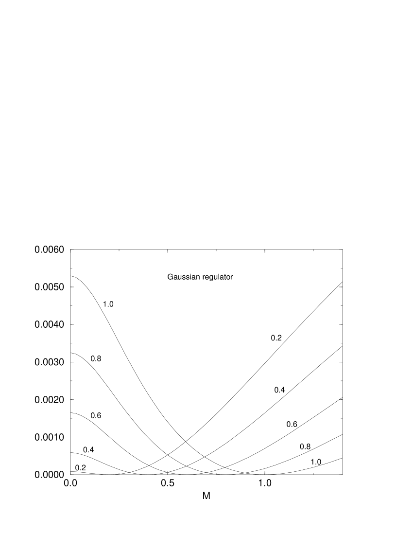
Figure 1: The classical effective potential calculated with a gaussian regulator and plotted as a function of $M$, for various indicated values of $M_{0}/\Lambda$. The effective potential is expressed in units of $\Lambda^{4}$.

Figure 2 shows shows the classical effective potential (36) calculated with a sharp cut-off. The code can be checked against analytic expressions in this case. We see that for increasing values of $\frac{M_{0}}{\Lambda}$, that is, for decreasing values of the cut-off, the minimum of the effective potential at $M=M_{0}$ becomes increasingly shallower and that it disappears altogether at the critical value $\frac{M_{0}}{\Lambda}\geq 0.\,742\quad$which can be evaluated analytically. When a gaussian regulator is used, the onset of the instability occurs at the much higher value $\frac{M_{0}}{\Lambda}\geq 2.93$ which was evaluated numerically.

The system appears to display an instability with respect to perturbations caused by the constraint $\frac{1}{2}j\left(\bar{\psi}\Gamma_{a}\psi\right)^{2}$. Furthermore, the energy of the system does not seem bounded from below. It goes without saying that the classical action (as opposed to the classical effective potential) displays a minimum at $M=M_{0}$ for all values of $M_{0}/\Lambda$.

Figure 2: The classical effective potential, calculated with a sharp 4-momentum cut-off, and plotted as a function of $M$ for various indicated values of $M_{0}/\Lambda$. The effective potential is expressed in units of $\Lambda^{4}$.

Let us take a closer look at this apparent instability. It is not an artefact of the classical approximation. Figure 3 shows the various contributions to the effective potential when the $1/N_{c}$ field fluctuations are included, using a sharp cut-off with $M_{0}/\Lambda=0.8$. We see that the field fluctuations lower the energy but that they do not significantly change the shape of the effective potential, so that the instability remains. We also see that the exchange (Fock) term dominates the $1/N_{c}$ corrections because it is more sensitive than the ring diagrams to the high momenta running in the meson loop. These conclusions remain valid for smaller values of $M_{0}/\Lambda$.

Figure 3: Various contributions to the effective potential calculated with a sharp cut-off with a value $M_{0}/\Lambda=0.8$. The energies are measured relative to the classical action at $M=M_{0}$.

By way of comparison, figure 4 shows the contributions of the $1/N_{c}$ corrections when a gaussian regulator is used. Although the effect of the meson fluctuations is somewhat larger, the stability of the system is not modified. We see however that the ring diagrams make a somewhat larger contribution than the exchange (Fock) term, because the gaussian regulator reduces the effect of the high momenta running in the meson loop. The same conclusions can be reached for different values of $\frac{M_{0}}{\Lambda}$. As mentioned above, the instability also occurs when a gaussian cut-off is used, but at much higher values of $M_{0}/\Lambda\geq 2.93$. For such high values, the cut-off is too small to be physically meaningful. With a gaussian regulator and in the relevant range of parameters $0.4<M_{0}/\Lambda<0.8$, one needs to probe the system with values as high as $M/\Lambda>4$ before it becomes apparent that the energy is not bounded from below.

Figure 4: Various contributions to the effective potential calculated with a gaussian regulator and with $M_{0}/\Lambda=0.8$. The energies are measured relative to the classical action at $M=M_{0}$.

A clue concerning the nature of the instability can be obtained by considering the effective potential obtained with a sharp 3-momentum regularisation. In this regularization, the trace of the quark loop is calculated by integrating the energy variable from $-\infty$ to $+\infty$, and by limiting the 3-momentum by the condition $\left|\vec{k}\right|<\Lambda$. This regularization is tantamount to a limitation of the quantum mechanical Hilbert space available to the quarks. Figure 5 shows that the effective potential, calculated with a sharp 3-momentum cut-off, behaves as expected and that it does not display the instability.

Figure 5: The classical effective potential calculated with a sharp 3-momentum cut-off, for various indicated values of $M_{0}/\Lambda$. No instability appears.

11 Unphysical poles of the quark propagator.

The fact that the effective potential, calculated with a sharp 4-momentum cut-off, displays an instability that does not occur when a sharp 3-momentum cut-off is used, can be understood as an effect of the unphysical poles of the quark propagator which are introduced by the 4-momentum regulator. For constant fields, the quark propagator can be written in the form:

$$\frac{1}{k_{\mu}\gamma_{\mu}+r^{2}M}=\frac{-k_{\mu}\gamma_{\mu}+r_{k}^{2}M}{\omega^{2}+\vec{k}^{2}+r_{k}^{4}M^{2}}\quad\quad\quad\left(k_{\mu}=\left(\omega,\vec{k}\right)\right)$$ (60)

When a 3-momentum regularisation is used, we have $r_{k}^{2}=1$ when $\left|\vec{k}\right|<\Lambda$ and $r_{k}^{2}=0$ otherwise. In the complex $\omega$-plane, the quark propagator has only on-shell poles at $\omega=\pm i\sqrt{\vec{k}^{2}+M^{2}}$.

However, when a 4-momentum regulator is used, the quark propagator acquires extra poles, which also occur when proper-time regularization is used [16]. Such poles are unphysical in the sense that, taken seriously, they lead to instabilities of the vacuum. Equivalently one can say that the system behaves as if it was governed by a non-hermitian hamiltonian. This is sometimes also expressed by saying that the theory becomes acausal. We assign the cause of the instability discussed above to the existence of such unphysical poles. When the 4-momentum cut-off is high (and $M_{0}/\Lambda$ correspondingly low) the effect of these unphysical poles is not felt. But this is not the case in low energy hadronic physics where the parameter $M_{0}/\Lambda$ is in the range $0.4<M_{0}/\Lambda<0.8$. Furthermore, the position (and therefore the effect) of the unphysical poles depends very much on the shape of the regulator.

A qualitative understanding of the difference between a sharp 4-momentum cut-off and a soft gaussian regulator can be understood by comparing the location of the poles of the quark propagator in the complex $k^{2}$ plane. When a gaussian regulator is used, the poles of the quark propagator occur when:

$$k^{2}+M^{2}e^{-\frac{2k^{2}}{\Lambda^{2}}}=0$$ (61)

Poles on the real axis of the complex $k^{2}$ plane occur only if $M^{2}<\frac{\Lambda^{2}}{2}$. Otherwise and in addition, poles occur in the complex plane. Figure 6 shows the poles of the quark propagator in the two cases $M/\Lambda=0.2$ (large cut-off) and $M/\Lambda=0.8$ (small cut-off). The poles all lie to the left of the imaginary axis and they move closer to it when the cut-off gets small. Table 5 gives the residues of the poles.

$\frac{M}{\Lambda}$ ${\rm Re}k^{2}$ ${\rm Im}k^{2}$ residue $\frac{M}{\Lambda}$ ${\rm Re}k^{2}$ ${\rm Im}k^{2}$ residue 0.2 -0.044 0 $\allowbreak 1.1\,0$ 0.8 -0.072 $\pm 0.74$ $0.\,29\mp i\,\,0.\,51$ 0.2 -1.941 0 $-0.\,35$ 0.8 -0.906 $\pm 3.81$ $-0.01\,4\mp i\,\,0.\,13$ 0.2 -2.342 $\pm 3.64$ $-0.05\,5\mp i\,0.\,11$ 0.8 -1.202 $\pm 6.98$ $-0.007\,1\mp i\,\,0.071$ 0.2 -2.607 $\pm 6.89$ $-0.02\,0\mp i\,0.06\,6$ 0.8 -1.386 $\pm 10.14$ $-0.004\,3\mp i\,\,0.04\,9$ 0.2 -2.783 $\pm 10.08$ $-0.01\,1\mp i\,\,0.04\,7$

Table 5: Position and residues of the poles of the quark propagator with a gaussian regulator. Values are given for $M/\Lambda=0.2$ and $0.8$

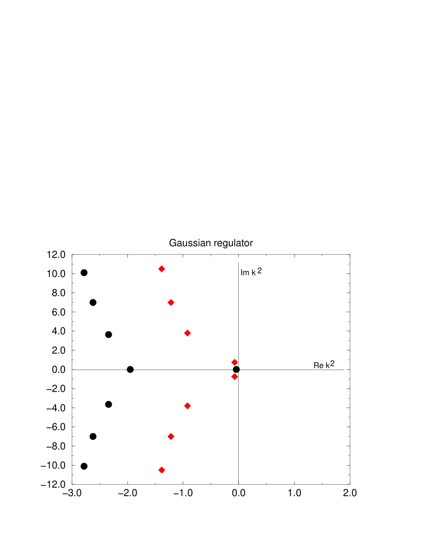
Figure 6: The poles of the quark propagator with a gaussian regulator in the complex $k^{2}$ plane. The circles are for $M/\Lambda=0.2$ and the diamonds are for $M/\Lambda=0.8$.

Consider next regularisation using a sharp 4-momentum cut-off. The corresponding regulator does not have an analytic form, but we have checked that very similar results are obtained with a Wood-Saxon shaped regulator $r_{k}^{4}=\frac{1}{1+e^{\frac{k^{2}-\Lambda^{2}}{c}}}$ which becomes equivalent to a sharp cut-off when $c\rightarrow 0$. The poles of the quark propagator are then the solution of the the equation:

$$k^{2}+\frac{M^{2}}{1+e^{\frac{k^{2}-\Lambda^{2}}{c}}}=0$$ (62)

Setting $k^{2}=x+iy$, this equation decomposes into the two equations:

$$x+M^{2}\frac{1+e^{\frac{x-\Lambda^{2}}{c}}\cos\frac{y}{c}}{\left(1+e^{\frac{x-\Lambda^{2}}{c}}\cos\frac{y}{c}\right)^{2}+\left(e^{\frac{x-\Lambda^{2}}{c}}\sin\frac{y}{c}\right)^{2}} = 0$$ (63)

$$y-M^{2}\frac{e^{\frac{x-\Lambda^{2}}{c}}\sin\frac{y}{c}}{\left(1+e^{\frac{x-\Lambda^{2}}{c}}\cos\frac{y}{c}\right)^{2}+\left(e^{\frac{x-\Lambda^{2}}{c}}\sin\frac{y}{c}\right)^{2}} = 0$$ (64)

One pole occurs on the negative real axis $\left(y=0\quad x\approx-M^{2}\right)$ in the vicinity of $-M^{2}$. It is simple to see that the complex poles all occur in the vicinity of the line $x=\Lambda$. The imaginary part $y$ is then the solution of the equation:

$$\frac{y}{2c}=\frac{M^{2}}{4c}\tan\frac{y}{2c}$$ (65)

The spacing between the poles is thus close to $2\pi c$ so that they get denser in number as $c\rightarrow 0$. In that limit, the continuum of poles forms a cut which expresses the discontinuity of the regulator when a sharp cut-off is used. A more exact numerical calculation of the position and residues of the poles is given in the table 6 for the case where $c=0.05$ $\Lambda^{2}$ and $M/\Lambda=0.8$.

$M/\Lambda=0.8\quad c/\Lambda^{2}=0.05\,$ $x$ $y$ residue $M=0.8\quad c=0.05$ -0.64000 0 1 $M=0.8\quad c=0.05$ 1.02152 $\pm 0.46354$ $-0.02\,7646\pm 0.007\,3992i$ $M=0.8\quad c=0.05$ 1.01790 $\pm 0.77472$ $-0.02\,4736\pm 0.01\,1194i$ $M=0.8\quad c=0.05$ 1.01431 $\pm 1.08764$ $-0.02\,1203\pm 0.01\,3627i$ $M=0.8\quad c=0.05$ 1.01128 $\pm 1.401618$ $-0.01\,7739\pm 0.0\,148i$

Table 6: Position and residues of the first few poles the quark propagator when a Wood-Saxon shaped regulator with $c=0.05$ $\Lambda^{2}$ and $M/\Lambda=0.8$.

The unphysical poles produced by a soft gaussian regulator lie to the left of the imaginary axis of the complex $k^{2}$ plane. They are therefore mostly felt at low values of $k^{2}$ where phase space factors reduce their effect. The unphysical poles produced by a sharp cut-off lie close to the boundary $k^{2}=\Lambda^{2}$ of high values of $k^{2}$ from which diverging quantities derive most of their contribution. This explains qualitatively the difference between the effect of the two regularizations on the effective potential. It would be worth analyzing whether the instabilities, recently heralded by Kleinert et al.[Kleinert], are not also artefacts of the use of a sharp 4-momentum in conjunction with a low cut-off.

12 Conclusions.

Although the meson loop contributions do not modify appreciably the value of the quark condensate, they do cause large quantum fluctuations of the quark condensate. The Lorentz invariant regularization of the quark propagator, used in conjunction with the relatively low cut-off values required in low energy hadronic physics, makes the physical vacuum unstable against distortions caused by the squared quark condensate. The instability depends strongly on the shape of the regulator. It is only weakly felt when a soft gaussian regulator is used but its effects are greatly enhanced in calculations which use a sharp 4-momentum cut-off. Large errors can be made if loop integrals are regularized after being derived from an unregularized action, instead of including the regulator in the model action from the outset. The ground state instability can be traced to unphysical poles of the quark propagator which are introduced by the regulator.

Appendix A Expressions for the classical action and the classical effective action.

In the chiral limit, the value of the classical action at the stationaty point is:

$$I_{j,m=0}\left(M^{2}\right)-I\left(M_{0}^{2}\right)$$ (A.1)

$$=\frac{1}{2}4N_{c}N_{f}\frac{\Omega}{\left(2\pi\right)^{4}}\int d_{4}k\left(-\ln\frac{k^{2}+r_{k}^{4}M^{2}}{k^{2}+r_{k}^{4}M_{0}^{2}}+\,\,\frac{r_{k}^{4}M^{2}}{k^{2}+r_{k}^{4}M^{2}}-\frac{r_{k}^{4}M_{0}^{2}}{k^{2}+r_{k}^{4}M_{0}^{2}}\right)$$ (A.2)

We measure all energies relative to the minimum $I\left(M_{0}^{2}\right)$ of the classical action in the unconstrained system where $j=0$. In units of $\Omega\Lambda^{4}$, the classical action depends only on the two variables $\frac{M}{\Lambda}$ and $\frac{M_{0}}{\Lambda}$.

Appendix B Expressions for the meson propagators.

B.1 The meson propagators $K_{ab}^{-1}$ and the polarization function $\Pi_{a}$ at a point $\varphi_{a}=\left(M,0,0,0\right)$.

From the second order expansion of $-Tr\ln\left(-i\partial_{\mu}\gamma_{\mu}+r\varphi_{a}\Gamma_{a}r\right)$ we obtain the following expression for the polarization function:

$$\Pi^{\left(2\right)}\left(\delta\varphi\right)=\frac{1}{2}Tr\frac{1}{-i\partial_{\mu}\gamma_{\mu}+r^{2}M}r\delta\varphi_{a}\Gamma_{a}r\frac{1}{-i\partial_{\mu}\gamma_{\mu}+r^{2}M}r\delta\varphi_{a}\Gamma_{a}r$$ (B.1)

The calculation is standard. Taking traces over the Dirac and flavor indices, and keeping track of the regulator, we obtain:

$$\Pi^{\left(2\right)}=4N_{c}N_{f}\frac{1}{2\Omega}\sum_{q}\delta S\left(q\right)\delta S\left(-q\right)\left(\frac{1}{2}q^{2}f_{M}^{22}\left(q\right)+M^{2}\left(f_{M}^{26}\left(q\right)+f_{M}^{44}\left(q\right)\right)-g_{M}\left(q\right)\right)$$

$$+4N_{c}N_{f}\frac{1}{2\Omega}\sum_{q}\delta P_{i}\left(q\right)\delta P_{i}\left(-q\right)\left(\frac{1}{2}q^{2}f_{M}^{22}\left(q\right)+M^{2}\left(f_{M}^{26}\left(q\right)-f_{M}^{44}\left(q\right)\right)-g_{M}\left(q\right)\right)$$ (B.2)

where we wrote the fields $\varphi_{a}$ in terms of scalar and pseudoscalar fields $S$ and $P_{i}:$

$$\Gamma_{a}\varphi_{a}=S+i\gamma_{5}\tau_{i}P_{i}$$ (B.3)

The Fourier transforms are defined to be:

$$S\left(q\right)=\int d_{4}x\,\,e^{iq_{\mu}x_{\mu}}S\left(x\right)\quad\quad\quad P_{i}\left(q\right)=\int d_{4}x\,\,e^{iq_{\mu}x_{\mu}}P_{i}\left(x\right)$$ (B.4)

The function $f_{M}^{np}\left(q\right)$ is:

$$f_{M}^{np}\left(q\right)=\frac{4\pi}{\left(2\pi\right)^{4}}\int_{0}^{\infty}k^{3}dk\int_{0}^{\pi}d\alpha\sin{}^{2}\alpha\frac{r_{k_{1}}^{n}r_{k_{2}}^{p}}{\left(k_{1}^{2}+r_{k_{1}}^{4}M^{2}\right)\left(k_{2}^{2}+r_{k_{2}}^{4}M^{2}\right)}$$ (B.5)

with $k_{1}=k-\frac{q}{2}$ and $k_{2}=k+\frac{q}{2}$. The function $g_{M}\left(q\right)$ is:

$$g_{M}\left(q\right)=\frac{4\pi}{\left(2\pi\right)^{4}}\int_{0}^{\infty}k^{3}dk\int_{0}^{\pi}d\alpha\sin{}^{2}\alpha\frac{r_{k_{1}}^{2}}{k_{1}^{2}+r_{k_{1}}^{4}M^{2}}r_{k_{2}}^{2}$$ (B.6)

and we denote by $g_{M}$ the function $g_{M}\left(q=0\right)$.

It follows that the polarization function is diagonal in momentum space:

$$\left\langle qa\left|\Pi\right|q^{\prime}b\right\rangle=\delta_{ab}\delta_{qq^{\prime}}\Pi_{a}\left(q\right)$$ (B.7)

where:

$$\Pi_{a=0}\left(q\right)\equiv\Pi_{S}\left(q\right)=4N_{c}N_{f}\left(\frac{1}{2}q^{2}f_{M}^{22}\left(q\right)+M^{2}\left(f_{M}^{26}\left(q\right)+f_{M}^{44}\left(q\right)\right)-g_{M}\left(q\right)\right)$$

$$\Pi_{a=1,2,3}\left(q\right)\equiv\Pi_{P}\left(q\right)=4N_{c}N_{f}\left(\frac{1}{2}q^{2}f_{M}^{22}\left(q\right)+M^{2}\left(f_{M}^{26}\left(q\right)-f_{M}^{44}\left(q\right)\right)-g_{M}\left(q\right)\right)$$ (B.8)

The inverse propagator matrix $K^{-1}$ is obtained by adding $-\left\langle xa\left|\left(V-j\right)^{-1}\right|yb\right\rangle$. We use the gap equation (27) to write:

$$-\left(V-j\right)^{-1}=4N_{c}N_{f}\frac{M}{M-m}g_{M}$$ (B.9)

so that:

$$K_{S}^{-1}\left(q\right)=4N_{c}N_{f}\left(\frac{1}{2}q^{2}f_{M}^{22}\left(q\right)+M^{2}\left(f_{M}^{26}\left(q\right)+f_{M}^{44}\left(q\right)\right)-g_{M}\left(q\right)+\frac{M}{M-m}g_{M}\left(0\right)\right)$$

$$K_{P}^{-1}\left(q\right)=4N_{c}N_{f}\left(\frac{1}{2}q^{2}f_{M}^{22}\left(q\right)+M^{2}\left(f_{M}^{26}\left(q\right)-f_{M}^{44}\left(q\right)\right)-g_{M}\left(q\right)+\frac{M}{M-m}g_{M}\left(0\right)\right)$$ (B.10)

Acknowledgments.

The author wishes to thank W.Broniowski and B.Golli for numerous discussions, and J.Zinn-Justin and L.Pitaevskii for help in undestanding reference [11].

References

- [1] R.Tegen V.Dmitrasinovic, H.Schulze and R.Lemmer. Annals Phys. 238, page 332, 1995.
- [2] C.Christov G.Ripka E.Nikolov, W.Broniowski and K.Goeke. Nucl.Phys.. A608, page 411, 1996.
- [3] W.Florkowski and W.Broniowski. Melting of the quark condensate in the njl model with meson loops. H.Niewodniczanski Institute of Nuclear Physics preprint INP 1728/PH, hep-ph/9605315.
- [4] M.Oertel M.Bumballa and J.Wambach. Meson properties in the 1/n corrected njl model. hep-ph/0001239. In this paper they calculate several effects due to two pion and two sigma intermediate states. A very carefully performed calculation., 2000.
- [5] J.Huefner S.P.Klevansky, Y.B.He and P.Rehberg. Nucl.Phys. A630, page 719, 1998.
- [6] E.Shuryak. Nucl.Phys. B203, pages 93,116,140, 1982.
- [7] D.I.Diakonov and V.Y.Petrov. Nucl.Phys. B272, page 457, 1986.
- [8] D.I.Diakonov C.Weiss and M.V.Polyakov. Nucl.Phys. B461, page 539, 1996.
- [9] W.Broniowski B.Golli and G.Ripka. Phys.Lett. B437, page 24, 1998.
- [10] R.S.Plant and M.C.Birse. Nucl.Phys. A628, page 607, 1998.
- [11] W.Broniowski. Mesons in non-local chiral quark models. hep-ph/9911514. 1999.
- [12] B.Szczerbinska and W.Broniowski. Acta Pol. 31, page 835, 2000.
- [13] C.Itzykson and J.B.Zuber. Quantum Field Theory. McGraw Hill, 1980.
- [14] H.Kleinert and B.Van Den Boosche. No massless pions in the nambu jona-lasinio model due to chiral fluctuations. hep-ph/9908284. 1999.
- [15] E.Babaev. On symmetry breakdown in njl … hep-th/9909052. 2000.
- [16] E.N.Nikolov W.Broniowski, G.Ripka and K.Goeke. Zeit.Phys. A354, page 421, 1996.