Non-Fermi Liquid Behaviour, the BRST Identity in the Dense Quark-Gluon Plasma and Color Superconductivity.

Abstract

At sufficiently high baryon densities, the physics of a dense quark-gluon plasma may be investigated through the tools of perturbative QCD. This approach has recently been successfully applied to the study of color superconductivity, where the dominant di-quark pairing interaction arises from one gluon exchange. Screening in the plasma leads to novel behaviour, including a remarkable non-BCS scaling of $T_{C}$, the transition temperature to the color superconducting phase. Radiative corrections to one gluon exchange were previously considered and found to affect $T_{C}$. In particular, the quark self-energy in a plasma leads to non-Fermi liquid behaviour and suppresses $T_{C}$. However, at the same time, the quark-gluon vertex was shown not to modify the result at leading order. This dichotomy between the effects of the radiative corrections at first appears rather surprising, as the BRST identity connects the self-energy to the vertex corrections. Nevertheless, as we demonstrate, there is in fact no contradiction with the BRST identity, at least to leading log order. This clarifies some of the previous statements on the importance of the higher order corrections to the determination of $T_{C}$ and the zero temperature gap in color superconductivity.

I Introduction.

Attention to the physics of a dense quark-gluon plasma has recently been revived, along with progress in understanding the phase structure of QCD. Interest has only heightened recently with the projected onset of relativistic heavy ion collisions at BNL. Such unusual conditions of QCD may also exist in nature, for example in the core of a dense neutron star. The asymptotic freedom of QCD makes a perturbative treatment applicable at sufficiently high baryon density, and the attractive di-quark interaction mediated by one gluon exchange in the antisymmetric color representation induces superconductivity below a certain temperature [1, 2, 3, 4, 5, 6, 7].

Working at non-zero temperature and chemical potential introduces several complications. One of the primary features of the plasma is that it screens the QCD interaction. Thus it is necessary in principle to dress gluon propagators with hard dense/thermal loops (HDL/HTL) in the plasma. For conditions in the range of interest for color superconductivity, the temperature effects are less important, and only the effects of screening by HDL need to be considered. That this screening is important is a corollary of a more general statement, namely that, with a long range interaction at non-zero chemical potential, a straightforward power series expansion of the free energy in the coupling $g$ results in infra-red divergences. A resummation over the fermion loops, and the replacement of the bare gluon propagator by that dressed with HDL [8, 9, 10], prior to perturbative expansion resolves the infra-red difficulties. This was demonstrated, for example, for a non-relativistic electron gas with Coulomb interaction in [11]. The resultant perturbative series contains logarithms of the coupling constant accompanying the powers of it.

As a result of HDL, the electric gluon propagator is screened effectively by a Debye mass, $m_{D}$, while the magnetic propagator is poorly screened via Landau damping in the sensitive region of momentum space. An important consequence of this is the introduction of non-Fermi liquid behavior of the quark self-energy [12]. In the infra-red limit (highlighted by a cutoff $l_{c}$) this self-energy is

$$\Sigma(\nu,\vec{p}\,)|_{p=\mu}\simeq-\frac{ig^{2}}{12\pi^{2}}C_{f}\gamma_{4}\,\nu\ln\frac{4l_{c}^{3}}{\pi m_{D}^{2}|\nu|},$$ (1)

where $(\vec{p},\nu)$ are the Euclidean energy-momentum. Such a non-analytic dependence on energy $\nu$ was first discovered in solid state physics [13] in the context of magnetic interactions. The logarithm suppresses the quasi-particle weight at the Fermi level and the single fermion occupation number becomes a continuous function at $p=p_{F}$, the Fermi momentum, in contrast to the kink of a Fermi liquid. Another effect is a term $\sim T\ln T$ in the specific heat, but this turns out to be too small to be observed since the magnetic coupling represents merely a relativistic correction. Such non-analyticity as indicated by (1) was also suggested for certain strongly correlated systems such as high $T_{C}$ superconductors [14].

In a relativistic quark-gluon plasma, the relatively poor screening by Landau damping is far more transparent. The di-quark pairing force is dominated by magnetic gluons, and Landau damping gives rise to a remarkable non-BCS scaling of the transition temperature and the energy gap for color superconductivity [12, 15, 16, 17],

$$k_{B}T_{C}=c\frac{\mu}{g^{5}}e^{-\sqrt{\frac{6N_{c}}{N_{c}+1}}\frac{\pi^{2}}{g}}.$$ (2)

The non-Fermi liquid behavior (1) suppresses the pre-exponential factor $c$ significantly, and we found that [18]

$$c=c_{0}e^{-\frac{1}{16}(\pi^{2}+4)(N_{c}-1)}\simeq 0.176\,c_{0}\qquad\hbox{for $N_{c}=3$},$$ (3)

with $c_{0}$ the pre-exponential factor without radiative corrections [15, 16, 19, 20]. We have also argued that the contributions from other higher order diagrams to (3) are subleading.

Since the inverse quark propagator is related to the quark-gluon vertex function through a BRST identity, so is the quark self-energy $\Sigma(P)$ of Fig. 1 to the radiative correction $\Lambda_{\mu}^{l}(P^{\prime},P)$ of Fig. 2. To illustrate such a relation, we focus on the vertex correction in Fig. 2a, which survives in the abelian case and will be referred to as the ‘abelian’ vertex in the following. After factorizing out the group theoretic coefficients from the vertex and self-energy,

$$\Lambda_{\mu}^{l(a)}(P^{\prime},P)=gT_{f}^{m}T_{f}^{l}T_{f}^{m}\Lambda_{\mu}(P^{\prime},P)$$ (4)

and

$$\Sigma(P)=T_{f}^{l}T_{f}^{l}\Xi(P),$$ (5)

we have the Takahashi identity

$$(P^{\prime}-P)_{\mu}\Lambda_{\mu}(P^{\prime},P)=\Xi(P^{\prime})-\Xi(P).$$ (6)

Taking the limit $P^{\prime}\to P$, we end up with the usual Ward identity,

$$\Lambda_{\mu}(P,P)=\frac{\partial}{\partial P_{\mu}}\Xi(P),$$ (7)

which is similar to the Ward identity of QED. Because of the above behavior of $\Xi(P)$, this identity raises a suspicion that $\Lambda_{\mu}(P^{\prime},P)$ must also contribute to the pre-exponential factor in a manner similar to (3). This was, however, ruled out in [18] where we showed that while the derivative $\frac{\partial}{\partial\nu}\Xi(P)$ contains the logarithm of $\nu$, the derivative $\frac{\partial}{\partial p_{i}}\Xi(P)$ does not, and thus the effect is not that of wave function renormalization. The contribution of $\Lambda_{4}(P^{\prime},P)$ remains subleading even with the logarithm since the Coulomb propagator attached to it is strongly screened.

Nevertheless a paradox arises here. The integral representations of $\Lambda_{i}(P,P)$ and $\Lambda_{4}(P,P)$ look identical while the above results, together with (7), suggests different answers. In this article we shall disentangle this mystery. It turns out that the expression $\Lambda_{\mu}(P,P)$ is highly ambiguous in the presence of a Fermi sea, and in particular,

$$\lim_{\vec{p}\,^{\prime}\to\vec{p}}\lim_{\nu^{\prime}\to\nu}\Lambda_{\mu}(P^{\prime},P)\neq\lim_{\nu^{\prime}\to\nu}\lim_{\vec{p}\,^{\prime}\to\vec{p}}\Lambda_{\mu}(P^{\prime},P),$$ (8)

a common ambiguity of the infra-red limit (the zero energy-momentum limit of soft lines of a diagram) in the absence of covariance. The contribution of $\Lambda_{\mu}^{l}(P^{\prime},P)$ to color superconductivity comes mainly in the region $|\nu^{\prime}-\nu|\ll\mu$ with $|\vec{p}\,^{\prime}-\vec{p}\,|\sim m_{D}^{2/3}|\nu^{\prime}-\nu|^{1/3}$ while $|p-\mu|\sim|\nu|$ and $|p^{\prime}-\mu|\sim|\nu^{\prime}|$, which is closer to the order of the left hand side of (8). By carefully tracing the subtleties of the infra-red limit along the different routes, we are able to reconcile the logarithmic behavior of (1) with the Ward identity (7) as well as the full BRST identity when the group theoretic factors and the vertex diagrams in Fig. 2b and Fig. 2c are restored. Yet the suppression in (3) remains intact.

Though we are mainly addressing QCD and color superconductivity in this article, the non-Fermi liquid behavior of the fermion self-energy and the vertex function apply, to a simpler extent, to the relativistic electron plasma as well. Such a plasma exists inside a white dwarf star, a supernova or a red giant star, for which the condition that the chemical potential is much higher that the temperature is valid.

In the next section, we shall calculate the quark self-energy and pin down the mathematical mechanism behind the logarithm of (1). The vertex function $\Lambda_{\mu}^{l}(P^{\prime},P)$ is analyzed in section III in light of the BRST identity. The contribution to color superconductivity will be discussed in section IV together with some concluding remarks.

II The Quark Self-Energy.

FIG. 1.: The quark self-energy diagram.

Little motivation is required for the analysis of the quark self-energy, represented in Fig. 1; it may appear as a simple radiative correction in perturbative processes, but it also enters the BRST identity. The form of the self-energy also characterises the non-Fermi liquid behaviour at high density and has a subtle influence over the divergences of the quark vertices. Without more ado, in Euclidean space we write,

$$\Sigma(P)=-g^{2}T_{f}^{l}T_{f}^{l}\frac{1}{\beta}\sum_{n}\int\frac{d^{3}\vec{l}}{(2\pi)^{3}}{\mathcal{D}}_{\mu\nu}(L)\gamma_{\mu}S(L+P)\gamma_{\nu},$$ (9)

where $L=(\vec{l},-\omega_{n})$, $P=(\vec{p},-\nu_{n})$, $\omega_{n}=n\epsilon$, $\nu_{n}=\left(n+\frac{1}{2}\right)\epsilon$, $\epsilon=2\pi k_{B}T$ and $T_{f}^{l}T_{f}^{l}=C_{f}=\frac{N_{c}^{2}-1}{2N_{c}}$ for $T_{f}$ in the fundamental representation of $SU(N_{c})$. Following the notation of [18, 20], we write the quark propagator as

$$S(P)=\frac{i}{/\kern-8.0ptP},$$ (10)

where $/\kern-8.0ptP=\gamma_{4}(\mu+i\nu)-i\vec{\gamma}\cdot\vec{p}$. In the presence of a Fermi sea it is necessary to incorporate HDL into the gluon propagator at leading order. While it is possible that a magnetic mass of order $T$ exists, at high density $\mu\gg k_{B}T$ the damping due to HDL prevails over that due to HTL [21]. Incorporating HDL, the gluon propagator in the covariant gauge takes the form

$${\cal D}_{\mu\nu}(K)=\frac{-i}{K^{2}+\sigma^{M}(k,\omega)}P_{\mu\nu}^{T}+\frac{-i}{K^{2}[1+\sigma^{E}(k,\omega)/k^{2}]}P_{\mu\nu}^{L}-i\alpha\frac{K_{\mu}K_{\nu}}{(K^{2})^{2}},$$ (11)

where $K=(\vec{k},-\omega)$, $K^{2}=k^{2}+\omega^{2}$, $P_{ij}^{T}=\delta_{ij}-\hat{k}_{i}\hat{k}_{j}$, $P_{i4}^{T}=P_{4j}^{T}=P_{44}^{T}=0$,

$$P_{\mu\nu}^{L}=\delta_{\mu\nu}-\frac{K_{\mu}K_{\nu}}{K^{2}}-P_{\mu\nu}^{T},$$ (12)

and $\alpha$ is the gauge parameter (we have adopted the notation $|\vec{k}\,|=k$). The electric self-energy $\sigma^{E}(k,\omega)$ and the magnetic self-energy $\sigma^{M}(k,\omega)$ in (11) are given by $\sigma^{E}(k,\omega)=m_{D}^{2}f^{E}\left(\omega/k\right)$, $\sigma^{M}(k,\omega)=m_{D}^{2}f^{M}\left(\omega/k\right)$, with $m_{D}^{2}\simeq\frac{N_{f}g^{2}\mu^{2}}{2\pi^{2}}$ and

$$f^{E}(x) = \left[1-x\tan^{-1}\left(\frac{1}{x}\right)\right],$$ (13)

$$f^{M}(x) = \frac{x}{2}\left[(1+x^{2})\tan^{-1}\left(\frac{1}{x}\right)-x\right].$$ (14)

For more discussion of our notation or HDL in general see [18, 20] or [21], respectively. From (13) we can see that the Coulomb interaction is strongly screened while from (14) the magnetic interaction is not. In this paper, we shall be interested only in the leading infra-red behavior, which comes solely from magnetic gluon exchange, and so we shall neglect the electric contributions and regard

$${\cal D}_{\mu\nu}(K)\approx-i{\cal D}(k,\omega)P_{\mu\nu}^{T},$$ (15)

with

$${\cal D}(k,\omega)=\frac{1}{k^{2}+\omega^{2}+\sigma^{M}(k,\omega)}.$$ (16)

To focus upon the infra-red behavior, we separate the loop integral into two regions and rewrite the self-energy as

$$\Sigma(P)=C_{f}\left[\Xi^{<}(P)+\Xi^{>}(P)\right],$$ (17)

where the superscripts denote integration inside and outside the infra-red sensitive region: $0<l<l_{c}$, $-\omega_{c}<\omega_{n}<\omega_{c}$ with $l_{c},\omega_{c}\ll\mu$. We shall evaluate the infra-red sensitive region only,

$$\Xi^{<}(P)\simeq-\frac{g^{2}}{4\pi^{2}}\int_{0}^{l_{c}}dl\,l^{2}\int_{-1}^{1}d(\cos\theta)\frac{1}{\beta}\sum_{n}\frac{\gamma_{4}-i(\hat{l}\cdot\hat{p})^{2}\vec{\gamma}\cdot\hat{p}}{\xi-i(\omega_{n}+\nu_{m})}{\cal D}(l,\omega_{n}),$$ (18)

where $\xi=|\vec{l}+\vec{p}\,|-\mu$. Corrections due to the change from a discrete sum to an integral are sub-leading; they can be obtained using zeta-function techniques as demonstrated for similar processes in [20]. Thus, in pursuit of the leading order behavior only, we immediately move to the continuous energy limit with $k_{B}T\ll\nu_{m}\ll\omega_{c}$. Making the change of variables from $\theta$ to $\xi$,

$$\int_{-1}^{1}d(\cos\theta)[\gamma_{4}-i(\hat{l}\cdot\hat{p})^{2}\vec{\gamma}\cdot\hat{p}]\simeq\int_{\xi_{p}-l}^{\xi_{p}+l}\frac{d\xi}{l}\left[\gamma_{4}-i\frac{\mu^{2}}{l^{2}p^{2}}\left(\xi-\xi_{p}\right)^{2}\vec{\gamma}\cdot\hat{p}\right],$$ (19)

with $\xi_{p}=p-\mu$, we find,

$$\Xi^{<}(\nu,\vec{p}\,)\simeq-\frac{g^{2}}{8\pi^{3}}\int_{0}^{l_{c}}dl\,l\int_{-\omega_{c}}^{\omega_{c}}d\omega{\cal D}(l,\omega)F(\nu,p;l,\omega),$$ (20)

$$F(\nu,p;l,\omega)=\int_{\xi_{p}-l}^{\xi_{p}+l}d\xi\frac{\gamma_{4}-i\frac{\mu^{2}}{l^{2}p^{2}}\left(\xi-\xi_{p}\right)^{2}\vec{\gamma}\cdot\hat{p}}{\xi-i(\omega+\nu)}.$$ (21)

Fixing $p=\mu$ for the external lines and carrying out the integration over $\xi$, we have,

$$F(\nu,\mu;l,\omega)=2i\gamma_{4}\tan^{-1}\frac{l}{\omega+\nu}+2\frac{\omega+\nu}{l}\vec{\gamma}\cdot\hat{p}\left(1-{\omega+\nu\over l}\tan^{-1}\frac{l}{\omega+\nu}\right),$$ (22)

so that

$$\frac{\partial}{\partial\nu}F(\nu,\mu;l,\omega) = 2\pi i\gamma_{4}\delta(\nu+\omega)-\frac{2il}{(\omega+\nu)^{2}+l^{2}}\gamma_{4}$$ (24)

$$\qquad+\frac{2}{l}\left[-2\frac{\omega+\nu}{l}\tan^{-1}\frac{l}{\omega+\nu}+\frac{2(\omega+\nu)^{2}+l^{2}}{(\omega+\nu)^{2}+l^{2}}\right]\vec{\gamma}\cdot\hat{p},$$

where the delta function comes from the discontinuity of the inverse tangent function. We find the energy dependence of the self-energy by differentiating,

$$\left.\frac{\partial}{\partial\nu}\Xi^{<}(\nu,\vec{p}\,)\right|_{p=\mu}=g^{2}[A(\nu)+B(\nu)],$$ (25)

with

$$A(\nu)=-\frac{i}{4\pi^{2}}\gamma_{4}\int_{0}^{l_{c}}dl\frac{l}{l^{2}+\nu^{2}+m_{D}^{2}f^{M}\left(\frac{-\nu}{l}\right)}$$ (26)

and

$$B(\nu) = \frac{1}{4\pi^{3}}\int_{0}^{l_{c}}dl\int_{-\omega_{c}}^{\omega_{c}}d\omega{\cal D}(l,\omega)$$ (28)

$$\qquad\qquad\Biggl{\{}\frac{il}{(\omega+\nu)^{2}+l^{2}}\gamma_{4}-\frac{1}{l}\left[2\frac{\omega+\nu}{l}\tan^{-1}\frac{l}{\omega+\nu}+\frac{2(\omega+\nu)^{2}+l^{2}}{(\omega+\nu)^{2}+l^{2}}\right]\vec{\gamma}\cdot\hat{p}\Biggr{\}}.$$

Noting the asymptotic behavior, that $f^{M}(x)\simeq{\pi\over 4}|x|$ for $|x|\ll 1$, a scale $l_{0}$ may be introduced to divide the integration in $A(\nu)$ into two: $|\nu|\ll l_{0}\ll\left(m_{D}^{2}|\nu|\right)^{1/3}$. For $l<l_{0}$ we have the contribution,

$$\int_{0}^{l_{0}}dl\frac{l}{l^{2}+\nu^{2}+m_{D}^{2}f^{M}\left(\frac{\nu}{l}\right)}\leq\frac{1}{m_{D}^{2}}\int_{0}^{l_{0}}dl\frac{l}{f^{M}\left(\frac{\nu}{l}\right)}<\frac{1}{m_{D}^{2}f^{M}\left(\frac{\nu}{l_{0}}\right)}\int_{0}^{l_{0}}dl\,l\sim\frac{l_{0}^{3}}{m_{D}^{2}|\nu|}\ll 1.$$ (29)

All of the inequalities follow straightforwardly from the definition of $l_{0}$ except for the second, which is due to $f^{M}(\nu/l)$ being a monotonically decreasing function of $l$. Therefore, neglecting this subleading contribution, we find a logarithmic infra-red singularity in $A(\nu)$ arising from the second region (namely the region $l_{0}<l<l_{c}$). The integration $B(\nu)$ is finite in the limit $\nu\to 0$. We end up with

$$\left.\frac{\partial}{\partial\nu}\Xi^{<}(\nu,\vec{p}\,)\right|_{p=\mu}=-\frac{ig^{2}}{4\pi^{2}}\gamma_{4}\int_{l_{0}}^{l_{c}}dl\frac{l^{2}}{l^{3}+\nu^{2}l+{\pi\over 4}m_{D}^{2}|\nu|}\simeq-\frac{ig^{2}}{12\pi^{2}}\gamma_{4}\ln\frac{4l_{c}^{3}}{\pi m_{D}^{2}|\nu|}+\cdots.$$ (30)

That the self-energy does not depend upon the spatial momentum in the infra-red limit can easily be ascertained by differentiating $\Xi(P)$ with respect to $p_{i}$. Noting that $\frac{\partial}{\partial p_{i}}=\hat{p}_{i}\frac{\partial}{\partial\xi_{p}}$, from (20) and (21) it is straightforward to find,

$$\left.\frac{\partial}{\partial\xi_{p}}\Xi^{<}(\nu,\vec{p}\,)\right|_{p=\mu}=ig^{2}B(\nu),$$ (31)

which is both real and finite in the limit $\nu\to 0$. Therefore the logarithmic singularity can not be attributed to a wavefunction renormalization. This is also the case found in a solid state physics context [13].

To summarise, we find that in a dense quark-gluon plasma the quark self-energy exhibits non-analytic behavior only for the energy component,

$$\left.\Sigma(P)\right|_{p=\mu}=-\frac{ig^{2}}{12\pi^{2}}C_{f}\gamma_{4}\,\nu\ln\frac{4l_{c}^{3}}{\pi m_{D}^{2}|\nu|}+\cdots$$ (32)

(the imaginary part of the self-energy, contributing to damping in the plasma [22, 23], is analytic as $\nu\to 0$). It is important to note that the infra-red non-analyticity in the energy originates in the discontinuity of the pole cutting the contour in the $\xi$ integration. This feature gives rise to the $\delta$-function in (24) which ultimately leads to the infra-red non-analyticity. This behavior will be seen to repeat itself in section IIIA where it will lead to infra-red divergences in the radiative corrections to the quark-gluon vertex.

From the result (32) it is clear that covariance is broken; this is a direct effect of the presence of a Fermi sea. We also see that $\Xi^{<}(0)=0$, so that the self-energy leads to no chemical potential renormalisation from the infra-red side. What is also of considerable interest is the BRST identity. How this is met in the dense quark-gluon plasma is subtle and we investigate this phenomenon in the next section.

III The BRST Identity at High Density.

Since the quark self-energy is only non-analytic in the external energy, one may expect from a generalisation of the Ward identity of QED that the Coulomb-quark vertex has similar behavior and is divergent while the magnetic gluon-quark vertex is not. However, it is also clear that the integrands in the infra-red region for $\Lambda_{4}^{l}$ and $\Lambda_{i}^{l}$ are mathematically identical, save for an indiced prefactor. Apparently we have something of a paradox: from the self-energy we expect only the Coulomb vertex to be divergent, but there appears to be no mathematical difference between the infra-red contribution to the Coulomb and magnetic vertices. We shall resolve this paradox in this section and show how the BRST identity works at high density. First of all, we shall examine the zero energy-momentum transfer limit of the abelian vertex $\Lambda_{\mu}(P^{\prime},P)$ and derive the precise expression of the Ward identity (7):

$$\lim_{\nu^{\prime}\to\nu}\lim_{\vec{p}\,^{\prime}\to\vec{p}}\Lambda_{4}(P^{\prime},P) = -\frac{\partial}{\partial\nu}\Xi(P),$$ (33)

$$\lim_{\vec{p}\,^{\prime}\to\vec{p}}\lim_{\nu^{\prime}\to\nu}\Lambda_{i}(P^{\prime},P) = \frac{\partial}{\partial p_{i}}\Xi(P).$$ (34)

The latter relation for the magnetic vertex was previously investigated in [24] for a system of fermions interacting with transverse abelian gauge bosons. Contrasting the Coulomb and magnetic cases in (33) provides an important clue hinting that the ordering of limits contributes to the subtlety we are overlooking. To show how the paradox is resolved this identity shall be considered in the next subsection, where the infra-red behavior of the vertices is discussed and the abelian vertex is treated in detail. In the second subsection we shall show how the full BRST identity works in the dense quark-gluon plasma in terms of Feynman diagrams.

A Infra-red Behavior of the Abelian Vertex.

To explore the behavior of the quark-gluon vertices and their relation to the BRST identity we shall analyse in detail the abelian vertex $\Lambda_{\mu}^{l(a)}$ shown in Fig. 2a. We refer to this vertex as ‘abelian’ since it is the only physical vertex that also appears in the abelian theory. In order to simplify matters further, in this subsection we shall put both external quarks on-shell, $p=p^{\prime}=\mu$.

Intuitively, we may expect the behavior of the vertex to depend subtly upon the ordering of the limits. We may develop this intuition from HDL, for example, where although there is an analytic result for the screening (13) and (14), it has different asymptotic behavior in the two orderings of the limits ($x\to 0$ and $x\to\infty$). As we shall see, HDL and the BRST identity at high density are intimately connected and it is no surprise that the ordering of limits in (33) is crucial in resolving the paradox. We write the abelian vertex as

$$\Lambda_{\mu}^{l(a)}(P^{\prime},P) = gT_{f}^{m}T_{f}^{l}T_{f}^{m}\Lambda_{\mu}(P^{\prime},P)$$ (35)

$$= gT_{f}^{l}\left(-{C_{ad}\over 2}+C_{f}\right)\Lambda_{\mu}^{(a)}(P^{\prime},P),$$ (36)

where

$$\Lambda_{\mu}^{(a)}(P^{\prime},P)=\frac{ig^{2}}{\beta}\sum_{n}\int\frac{d^{3}\vec{l}}{(2\pi)^{3}}{\cal D}_{\nu\rho}(l,\omega)\gamma_{\nu}S(L+P^{\prime})\gamma_{\mu}S(L+P)\gamma_{\rho}.$$ (37)

This may be written in terms of two integrals, one inside and one outside the infra-red sensitive region; $0<l<l_{c}$, $-\omega_{c}<\omega<\omega_{c}$ with $l_{c},\omega_{c}\ll\mu$,

$$\Lambda_{\mu}^{(a)}(P^{\prime},P)=\hat{P}_{\mu}\left[\Lambda^{(a)<}(P^{\prime},P)+\Lambda^{(a)>}(P^{\prime},P)\right].$$ (38)

with $\hat{P}_{\mu}=(-i\hat{p},1)$. In this subsection we are only interested in the leading infra-red behavior. So we evaluate,

$$\Lambda^{(a)<}(P^{\prime},P) \simeq \frac{g^{2}}{8\pi^{3}}\int_{0}^{l_{c}}dl\,l^{2}\int_{-1}^{1}d(\cos\theta)(\gamma_{4}-i\vec{\gamma}\cdot\hat{p}\cos^{2}\theta)\widetilde{\Lambda}(P,P^{\prime};L),$$ (39)

$$\widetilde{\Lambda}(P,P^{\prime};L) = \int\kern-10.0pt\circ\frac{d\omega}{2\pi}\frac{{\cal D}(l,\omega)}{\zeta^{\prime}-\zeta}\left(\frac{1}{\omega+\zeta^{\prime}}-\frac{1}{\omega-\zeta^{\prime}}-\frac{1}{\omega+\zeta}+\frac{1}{\omega-\zeta}\right)\ln(-\omega),$$ (40)

where $\zeta=\nu+i\xi$, $\xi=|\vec{l}+\vec{p}\,|-\mu$ and $\zeta^{\prime}$ and $\xi^{\prime}$ refer to $\nu^{\prime}$, $\vec{p}\,^{\prime}$. The logarithm in (40) introduces a branch cut which we may take to lie along the positive real axis and the contour to run above and below it in the normal fashion. As shown for the self-energy, it is only the discontinuities that occur as poles cut the contour and branch cut that induce the infra-red singularity. Hence we need only focus upon the second and fourth terms in (40), since the other terms are regular. Using the convention that ${\rm arg}(-1)=0$, we find that the contribution of these poles reads

$$\widetilde{\Lambda}_{\rm{disc.}}(P^{\prime},P;L)=\frac{\pi}{\zeta^{\prime}-\zeta}\left[{\rm Sign}(\xi){\cal D}(l,\zeta)-{\rm Sign}(\xi^{\prime}){\cal D}(l,\zeta^{\prime})\right],$$ (41)

where the sign function comes from the discontinuity of $\ln(-\omega)$ crossing the cut.

We are now in a position to take the limit $P_{\mu}\to P_{\mu}^{\prime}$ for the Ward identity and we shall consider the two different orderings of the limits in turn:

$${i)}~{}~{}\lim_{\nu^{\prime}\to\nu}\lim_{\vec{p}\,^{\prime}\to\vec{p}}\widetilde{\Lambda}_{\rm{disc.}}(P^{\prime},P;L) = -\pi{\rm Sign}(\xi)\frac{\partial}{\partial\nu}{\cal D}(l,\zeta),$$ (42)

$${ii)}~{}~{}\lim_{\vec{p}\,^{\prime}\to\vec{p}}\lim_{\nu^{\prime}\to\nu}\widetilde{\Lambda}_{\rm{disc.}}(P^{\prime},P;L) = i\pi\frac{\partial}{\partial\xi}\left[{\rm Sign}(\xi){\cal D}(l,\zeta)\right].$$ (43)

In both cases we are looking at the infra-red limit, and thus fix the external momentum to be $p=p^{\prime}=\mu$, $\xi_{p}=0$.

First of all, considering case $i$), using the change of variables (19) it is straightforward to find,

$$\left.\lim_{\nu^{\prime}\to\nu}\lim_{\vec{p}\,^{\prime}\to\vec{p}}\Lambda^{(a)<}(P^{\prime},P)\right|_{p=\mu} = -\frac{g^{2}}{8\pi^{2}}\int_{0}^{l_{c}}dl\,l\int_{-l}^{l}d\xi\>{\rm Sign}(\xi)\frac{\partial}{\partial\nu}{\cal D}(l,\zeta)(\gamma_{4}-i\frac{\xi^{2}}{l^{2}}\vec{\gamma}\cdot\hat{p})$$ (44)

$$= \frac{ig^{2}}{4\pi^{2}}\gamma_{4}\int_{0}^{l_{c}}dl\,l\left[{\cal D}(l,\nu)-{\cal D}(l,\nu+il)\right]+\cdots\$$ (45)

$$= \frac{ig^{2}}{12\pi^{2}}\gamma_{4}\ln\frac{4l_{c}^{3}}{\pi m_{D}^{2}|\nu|}+\cdots,$$ (46)

where the second term in the brackets of (45) contributes to the subleading terms denoted by ellipses in (46).

Secondly, considering case $ii$), we find that differentiation gives two terms which will cancel in the leading order,

$$\left.\lim_{\vec{p}\,^{\prime}\to\vec{p}}\lim_{\nu^{\prime}\to\nu}\Lambda^{(a)<}(P^{\prime},P)\right|_{p=\mu}=\frac{ig^{2}}{8\pi^{2}}\int_{0}^{l_{c}}dl\,l\int_{-l}^{l}d\xi (\gamma_{4}-i{\xi^{2}\over l^{2}}\vec{\gamma}\cdot\hat{p})$$ (48)

$$\times\left[{\rm Sign}(\xi)\frac{\partial}{\partial\xi}{\cal D}(l,\zeta)+2\delta(\xi){\cal D}(l,\zeta)\right].$$

The first term is identical to that evaluated for case $i$) above. With the same approximation, the second term is,

$$-\frac{ig^{2}}{4\pi^{2}}\int_{0}^{l_{c}}dl\frac{l^{2}}{l^{3}+{\pi\over 4}m_{D}^{2}|\nu|}\simeq-\frac{ig^{2}}{12\pi^{2}}\ln\frac{4l_{c}^{3}}{\pi m_{D}^{2}|\nu|}.$$ (49)

The two leading contributions cancel and in this ordering of limits the vertex is finite.

Now we can see how the paradox is resolved. The spatial abelian vertex considered with the ordering of the limits in case $ii$) is finite, in agreement with the second part of the identity (33).

B The BRST Identity.

The BRST identity is a generalisation of the Ward-Takahashi identities for non-abelian gauge theory obtained through the BRST transformations. The BRST version of the Takahashi identity can be written as,

$$(P^{\prime}-P)^{\mu}\Lambda_{\mu}^{l}(P^{\prime},P)=gT_{f}^{l}(\Sigma(P^{\prime})-\Sigma(P))+R^{l}(P^{\prime},P).$$ (50)

The physical quark-gluon vertices $\Lambda_{\mu}^{l}=\Lambda_{\mu}^{l(a)}+\Lambda_{\mu}^{l(b)}+\Lambda_{\mu}^{l(c)}$ are represented in Fig. 2. The non-physical ghost-quark vertices induced by the BRST transformation, $R^{l}=R^{l(a)}+R^{l(b)}+R^{l(c)}$, are represented in Fig. 3. They vanish for on-shell Minkowski momenta $P$ and $P^{\prime}$ at $\mu=0$.

The nontrivial part of the BRST identity (50) is in the dressing of the gluon lines of Figs. 1, 2 and 3 by HDL and the inclusion of Fig. 2c. The order of the perturbative expansion is mixed up without offsetting the simple form of the identity. The detailed derivation of (50) is given in Appendix A.

FIG. 2.: The physical radiative corrections to the quark-gluon vertex; $a$) $\Lambda_{\mu}^{l(a)}$, the abelian vertex, $b$) $\Lambda_{\mu}^{l(b)}$, the tri-gluon vertex and $c$) $\Lambda_{\mu}^{l(c)}$, the triangular vertex.

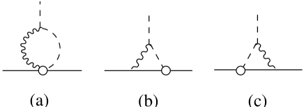
FIG. 3.: The non-physical ghost diagrams generated by the BRST transformations; representing $a$) $R^{l(a)}$, $b$) $R^{l(b)}$ and $c$) $R^{l(c)}$. The open circles denote non-physical vertices generated by BRST.

Setting $\vec{p}\,^{\prime}=\vec{p}$ on the Fermi level, the BRST identity (50) implies that

$$\lim_{\nu^{\prime}\to\nu}\left[\Lambda_{4}^{l}(P^{\prime},P)-\frac{R^{l}(P^{\prime},P)}{\nu^{\prime}-\nu}\right]_{\vec{p}\,^{\prime}=\vec{p},\;p=\mu} = -gT_{f}^{l}\frac{\partial}{\partial\nu}\Sigma(P)$$ (51)

$$= \frac{ig^{3}}{12\pi^{2}}C_{f}^{\vphantom{l}}T_{f}^{l}\gamma_{4}\ln\frac{4l_{c}^{3}}{\pi m_{D}^{2}|\nu|}.$$ (52)

It follows from the discussions of the previous subsection that $\Lambda_{4}^{l}(P^{\prime},P)=\Lambda_{4}^{l(a)}(P^{\prime},P)+\Lambda_{4}^{l(b)}(P^{\prime},P)+\Lambda_{4}^{l(c)}(P^{\prime},P)$ with

$$\Lambda_{4}^{l(a)}(P^{\prime},P)=gT_{f}^{l}\left(-\frac{C_{ad}}{2}+C_{f}\right)\frac{ig^{2}}{12\pi^{2}}\gamma_{4}\ln\frac{4l_{c}^{3}}{\pi m_{D}^{2}|\nu|}.$$ (53)

It remains to find the logarithmic terms from Figs. 2b, 2c or 3 to reconcile the BRST identity (50) to the leading order of the infrared logarithms.

For $\vec{p}\,^{\prime}=\vec{p}$ and $p=\mu$, we have

$$\Lambda_{4}^{l(b)}(P^{\prime},P) = ig^{3}f^{alb}T_{f}^{a}T_{f}^{b}\frac{1}{\beta}\sum_{n}\int\frac{d^{3}\vec{l}}{(2\pi)^{3}}(2\omega_{n}-\nu^{\prime}-\nu){\cal D}^{2}(l,\omega_{n})(\delta_{ij}-\hat{l}_{i}\hat{l}_{j})\gamma_{i}S(P+L)\gamma_{j}$$ (54)

$$= \frac{1}{2}gC_{ad}T_{f}^{l}[\Lambda_{4}^{(b)<}(P^{\prime},P)+\Lambda_{4}^{(b)>}(P^{\prime},P)],$$ (55)

where the superscripts specify the contributions from loop momentum inside and outside the infrared region, $|\omega|<\omega_{c}$ and $l<l_{c}$. The inside contribution can be approximated by

$$\Lambda_{4}^{(b)<}(P^{\prime},P) = \frac{g^{2}}{4\pi^{3}}\int_{0}^{l_{c}}dl\,l\int_{-\omega_{c}}^{\omega_{c}}d\omega\,\omega{\cal D}^{2}(l,\omega)\int_{-l}^{l}d\xi\frac{\gamma_{4}-i\frac{\xi^{2}}{l^{2}}\vec{\gamma}\cdot\hat{p}}{i(\omega+\nu)-\xi}$$ (56)

$$= -\frac{g^{2}}{2\pi^{3}}(iI_{i}\gamma_{4}+I_{2}\vec{\gamma}\cdot\hat{p}),$$ (57)

where

$$I_{1}=\int_{0}^{l_{c}}dl\,l\int_{-\omega_{c}}^{\omega_{c}}d\omega\,\omega{\cal D}^{2}(l,\omega)\tan^{-1}\frac{l}{\omega+\nu}$$ (58)

and

$$I_{2}=\int_{0}^{l_{c}}dl\,l\int_{-\omega_{c}}^{\omega_{c}}d\omega\,\omega{\cal D}^{2}(l,\omega)\left[\frac{\omega+\nu}{l}-\tan^{-1}\frac{l}{\omega+\nu}\right].$$ (59)

In the limit $\nu\to 0$, the integrand of both integrals $I_{1}$ and $I_{2}$ are positive and can be bounded by letting $\omega_{c}\to\infty$ and changing the integration variables from $(l,\omega)$ to $(l,x=\omega/l)$. We have

$$|I_{1}|\leq\int_{0}^{\infty}dx\frac{x\tan^{-1}{1\over x}}{(1+x^{2})^{2}}\left[\ln\frac{l_{c}^{2}(1+x^{2})}{m_{D}^{2}f^{M}(x)}-1\right]$$ (60)

and

$$|I_{2}|\leq\int_{0}^{\infty}dx\frac{x\left(x-\tan^{-1}{1\over x}\right)}{(1+x^{2})^{2}}\left[\ln\frac{l_{c}^{2}(1+x^{2})}{m_{D}^{2}f^{M}(x)}-1\right].$$ (61)

Both integrals are convergent and hence $\Lambda_{4}^{l(b)}$ does not contribute to the infrared logarithm. It is also straightforward to verify that the BRST generated diagrams in Fig. 3 do not display any logarithmic behavior in the limit $\nu\to 0$. Thus the only candidate left over is the diagram in Fig. 2c corresponding to gluon insertion on a HDL.

Though formidable as it looks, evaluation of Fig. 2c can be simplified with the aid of a Ward type identity which relates the derivative of the gluon self-energy and the tri-gluon vertex with three external gluon lines. Again the answer is sensitive to the relative order of the limits $\nu^{\prime}\to\nu$ and $\vec{p}\,^{\prime}\to\vec{p}$. In appendix B, we shall demonstrate that

$$\lim_{\nu^{\prime}\to\nu}\lim_{\vec{p}\,^{\prime}\to\vec{p}}\Lambda_{4}^{l(c)}(P^{\prime},P)=\frac{ig^{3}}{24\pi^{2}}C_{ad}T^{l}\gamma_{4}\ln\frac{4l_{c}^{3}}{\pi m_{D}^{2}|\nu|}+\cdots,$$ (62)

which completes the BRST identity (51) to the leading logarithm level. The other order of the limits, $\lim_{\nu^{\prime}\to\nu}\lim_{\vec{p}\,^{\prime}\to\vec{p}}\Lambda_{j}^{l(c)}(P^{\prime},P)$ is infrared finite.

To summarise, we have shown how the BRST identity works in a quark-gluon plasma at high density in terms of Feynman diagrams. The derivation of the identity is quite general and that it works at high density is not surprising, but with this presentation we hope that the mystery that shrouds this topic may be lifted. With the incorporation of HDL, the BRST identity is no longer satisfied order by order. The payment for using HDL is that orders of perturbation theory become mixed up.

IV Color superconductivity

Perturbative QCD has been applied successfully toward the study of color superconductivity at high baryon densities. In this regime, single gluon exchange dominates the pairing interaction, and screening plays an important role in the non-BCS behavior of color superconductivity [12, 15, 16, 17]. In Refs. [18, 20], the superconducting pairing temperature of a dense quark-gluon plasma was investigated by means of a Dyson-Schwinger approach to the pairing interaction. The resulting problem was reduced to one of finding the smallest eigenvalue, $\lambda$, of the Fredholm equation

$$f_{s_{1}^{\prime}s_{2}^{\prime}}(n^{\prime}|p^{\prime})=\frac{\lambda^{2}}{\beta}\sum_{n,s_{1},s_{2}}\int_{0}^{\infty}dp\,K_{s_{1}^{\prime}s_{2}^{\prime},s_{1}^{\vphantom{\prime}}s_{2}^{\vphantom{\prime}}}(n^{\prime},n|p^{\prime},p)f_{s_{1}s_{2}}(n|p),$$ (63)

with the condition $\lambda^{2}=1$ yielding the critical temperature. The kernel is given by

$$K_{s_{1}^{\prime}s_{2}^{\prime},s_{1}^{\vphantom{\prime}}s_{2}^{\vphantom{\prime}}}(n^{\prime},n|p^{\prime},p)=\frac{p^{2}}{2\pi}\sum_{s_{1}^{\prime\prime}s_{2}^{\prime\prime}}\gamma_{s_{1}^{\prime}s_{2}^{\prime},s_{1}^{\prime\prime}s_{2}^{\prime\prime}}(n^{\prime},n|p^{\prime},p)S_{s_{1}^{\prime\prime}s_{1}}(n|p)S_{s_{2}^{\prime\prime}s_{2}}(-n|p),$$ (64)

and consists of the $s$-wave components of the two particle irreducible amplitude for the scattering of two quarks in their color antisymmetric channel with zero total energy and momentum, $\gamma_{s_{1}^{\prime}s_{2}^{\prime},s_{1}^{\vphantom{\prime}}s_{2}^{\vphantom{\prime}}}(n^{\prime},n|p^{\prime},p)$, and the full quark propagator $S_{s^{\prime}s}(n|p)$. The initial energies of the two quarks are $\pm i\nu_{n}$ and the final ones are $\pm i\nu_{n^{\prime}}$ with $\nu_{n}=(n+\frac{1}{2})\epsilon$. The initial momenta of the two quarks are $\pm\vec{p}$ and the final ones are $\pm\vec{p}\,^{\prime}$. The diagrammatic expansion of $\gamma_{s_{1}^{\prime}s_{2}^{\prime},s_{1}^{\vphantom{\prime}}s_{2}^{\vphantom{\prime}}}(n^{\prime},n|p^{\prime},p)$ to order $g^{4}$ and $S_{s^{\prime}s}(n|p)$ to order $g^{2}$ is shown in Fig. 4.

FIG. 4.: The diagrammatic expansion of the two particle irreducible vertex $\Gamma_{s_{1}^{\prime}s_{2}^{\prime},s_{1}^{\vphantom{\prime}}s_{2}^{\vphantom{\prime}}}(n^{\prime},n|p^{\prime},p)$ to order $g^{4}$ and the quark self-energy $S_{s^{\prime}s}(n|p)$ to order $g^{2}$.

Collecting previous results, the perturbative expansion of the least eigenvalue reads [18, 20]

$$\frac{1}{\lambda^{2}} = {g^{2}\over 24\pi^{2}}\left(1+{1\over N_{c}}\right)\left[{4\over\pi^{2}}\log^{2}{2\over\hat{\epsilon}}+{8\over\pi^{2}}(\gamma+\log 2)\log{2\over\hat{\epsilon}}+{\cal O}(1)\right]$$ (66)

$$-\left({g^{2}\over 24\pi^{2}}\right)^{2}\left(1+{1\over N_{c}}\right)\left[C_{f}{4(\pi^{2}+4)\over\pi^{4}}\log^{3}{2\over\hat{\epsilon}}+{\cal O}(\log^{2}{2\over\hat{\epsilon}})\right]+{\cal O}(g^{6}),$$

where the leading ${\cal O}(g^{2})$ term stems from the first diagram of Fig. 4 with a bare quark propagator. Relative to this leading term, the radiative corrections and the two gluon exchange appear to be suppressed by $g^{2}$ as is the case with the remaining diagrams of Fig. 4, but may not be so because of the infra-red logarithm, each counted as $g^{-1}$ for $T\sim T_{C}$ in accordance with (2). The radiative correction to the quark propagator is such an example [12]. The logarithm of the self-energy, contained in the second line of (66), gives rise to a significant contribution to the prefactor [18]. Though the radiative correction to the vertex function is liable to such a logarithm according to the BRST identity, this does not happen in the energy momentum region $|p-\mu|\sim|\nu|$, $|p^{\prime}-\mu|\sim|\nu^{\prime}|$ and $|\vec{p}-\vec{p}\,^{\prime}|\sim(\kappa|\nu-\nu^{\prime}|)^{\frac{1}{3}}$, where the main contribution to the kernel (64) comes from; this is indicated by the absence of the logarithm in the limit $\nu^{\prime}\to\nu$ followed by $\vec{p}\,^{\prime}\to\vec{p}$ of the vertex function. In what follows, we shall demonstrate this point via an explicit evaluation of the contribution of the abelian vertex function to the partial wave amplitude.

Consider the abelian vertex Fig. 2a, with $p=p^{\prime}=\mu$, $q=2\mu\sin\frac{\theta}{2}\simeq\mu\theta$. The infra-red contribution is given by

$$\overline{\Lambda}_{j}^{(a)}(P^{\prime},P)=\overline{u}(P^{\prime})\Lambda_{j}^{(a)}(P^{\prime},P)u(P)$$ (67)

$$\kern 20.00003pt=g^{2}\hat{p}_{j}\int_{l<l_{c}}\frac{d^{3}\vec{l}}{(2\pi)^{3}}\int_{-\omega_{c}}^{\omega_{c}}\frac{d\omega}{2\pi}{\cal D}(l,\omega)\frac{\hat{p}\cdot\hat{p}^{\prime}-(\hat{p}\cdot\hat{l})(\hat{p}^{\prime}\cdot\hat{l})}{[i(\omega+\nu^{\prime})-\xi^{\prime}][i(\omega+\nu)-\xi]}$$ (68)

$$\kern 20.00003pt=g^{2}\hat{p}_{j}\int_{l<l_{c}}\frac{d^{3}\vec{l}}{(2\pi)^{3}}\int_{-\omega_{c}}^{\omega_{c}}\frac{d\omega}{2\pi}{\cal D}(l,\omega)\frac{\hat{p}\cdot\hat{p}^{\prime}-(\hat{p}\cdot\hat{l})(\hat{p}^{\prime}\cdot\hat{l})}{i\Delta\nu-\xi^{\prime}+\xi}\left[\frac{1}{i(\omega+\nu)-\xi}-\frac{1}{i(\omega+\nu^{\prime})-\xi^{\prime}}\right],$$ (69)

where $\Delta\nu=\nu^{\prime}-\nu$, $\xi=|\vec{p}+\vec{l}\,|-\mu$ and $\xi^{\prime}=|\vec{p}\,^{\prime}+\vec{l}\,|-\mu$ with $|\xi|\leq l$ and $|\xi^{\prime}|\leq l$. It follows from the discussions of the previous sections that the sensitive region of the integration variables which is responsible to the non-Fermi liquid logarithm corresponds to the singularities of the fractions inside the bracket. Therefore one of $\xi$ and $\xi^{\prime}$ must be kept small in the sensitive region. If there were an infra-red logarithm, it would come from

$$\overline{\Lambda}_{\eta}^{(a)}(P^{\prime},P)=\int_{l<l_{c}}\frac{d^{3}\vec{l}}{(2\pi)^{3}}\int_{-\omega_{c}}^{\omega_{c}}\frac{d\omega}{2\pi}\frac{{\cal D}(l,\omega)}{i\Delta\nu-\xi^{\prime}+\xi}\left[\frac{\theta(\eta l-|\xi|)}{i(\omega+\nu)-\xi}-\frac{\theta(\eta l-|\xi^{\prime}|)}{i(\omega+\nu)-\xi^{\prime}}\right],$$ (70)

with $\eta\ll 1$. Transforming the integration variables from $\vec{l}$ to $l$, $\xi$ and $\xi^{\prime}$, we have

$$d^{3}\vec{l}=\frac{\mu^{2}}{J}l\,dl\,d\xi\,d\xi^{\prime},$$ (71)

where the Jacobian is $J=|\vec{l}\cdot\vec{p}\times\vec{p}\,^{\prime}|\simeq\mu^{2}\sqrt{l^{2}\theta^{2}-(\xi-\xi^{\prime})^{2}}$ with the approximation that $\xi$ or $\xi^{\prime}\ll l$. Introducing

$$\overline{\cal D}(l,\omega)=\int_{-\infty}^{\omega}d\omega^{\prime}{\cal D}(l,\omega^{\prime}),$$ (72)

and carrying out the integration over $\xi$ and $\xi^{\prime}$, we obtain

$$\overline{\Lambda}_{\eta}^{(a)}(P^{\prime},P) = \frac{1}{8\pi^{2}}\int_{0}^{l_{c}}dl\frac{l}{\sqrt{l^{2}\theta^{2}+\Delta\nu^{2}}}\int_{-\omega_{c}}^{\omega_{c}}d\omega\overline{\cal D}(l,\omega)[\delta(\omega+\nu)-\delta(\omega+\nu^{\prime})]$$ (73)

$$= \frac{1}{8\pi^{2}}\int_{0}^{l_{c}}dl\frac{l}{\sqrt{l^{2}\theta^{2}+\Delta\nu^{2}}}\int_{-\nu^{\prime}}^{-\nu}d\omega{\cal D}(l,\omega).$$ (74)

Note that if $\vec{p}\,^{\prime}\to\vec{p}$ first, we have a complete exposure of $\Delta\nu$ in the denominator,

$$\overline{\Lambda}_{\eta}^{(a)}(P^{\prime},P)\simeq\frac{1}{8\pi^{2}}\frac{1}{\Delta\nu}\int_{0}^{l_{c}}dl\,l\int_{-\nu^{\prime}}^{-\nu}d\omega{\cal D}(l,\omega).$$ (75)

The integration will give rise to $\nu^{\prime}\ln|\nu^{\prime}|-\nu\ln|\nu|$, which in the limit $\nu^{\prime}\to\nu$ produces the infra-red logarithm. But here, with $\theta\sim|\nu^{\prime}-\nu|^{\frac{1}{3}}$ and $l\sim|\nu|^{\frac{1}{3}}$, such a singularity is suppressed through the $l^{2}\theta^{2}$ term inside of the square root. Indeed, if we insert $\Lambda_{\eta}^{(a)}(P^{\prime},P)$ into the partial wave integration, we find the corresponding contribution

$$\gamma_{IR}(\nu^{\prime},\nu)=\frac{g^{4}}{8\pi^{2}}\int_{0}^{\theta_{c}}d\theta\,\theta{\cal D}(\mu\theta,\nu^{\prime}-\nu)\int_{0}^{l_{c}}dl\frac{l}{\sqrt{l^{2}\theta^{2}+\Delta\nu^{2}}}\int_{-\nu^{\prime}}^{-\nu}d\omega{\cal D}(l,\omega).$$ (76)

$\gamma_{IR}(\nu^{\prime},\nu)$ may be bounded by dropping $\Delta\nu$ inside the square root. Then the integration over $\theta$ decouples from that over $l$ and $\omega$, i.e.

$$|\gamma_{IR}(\nu^{\prime},\nu)|\leq\frac{g^{4}}{8\pi^{2}}IJ,$$ (77)

where

$$I=\int_{0}^{\theta_{c}}d\theta{\cal D}(\mu\theta,\nu^{\prime}-\nu)$$ (78)

and

$$J=\int_{0}^{l_{c}}dl\int_{-\nu^{\prime}}^{-\nu}d\omega{\cal D}(l,\omega).$$ (79)

It follows from the properties of the function ${\cal D}(l,\omega)$ that $I$ and $J$ are bounded from above by

$$I\leq\frac{2\pi}{3\sqrt{3}\mu}(\kappa|\nu^{\prime}-\nu|)^{-\frac{1}{3}}$$ (80)

and

$$J\leq\frac{\pi}{\sqrt{3}}\kappa^{-\frac{1}{3}}||\nu^{\prime}|^{\frac{2}{3}}-{\rm{Sign}}(\nu^{\prime}\nu)|\nu|^{\frac{2}{3}}|,$$ (81)

where $\kappa={\pi\over 4}m_{D}^{2}$. Combining $I$ and $J$, we see that $\gamma_{IR}(\nu^{\prime},\nu)$ is nonsingular in the limit $\nu^{\prime}\to 0$ and $\nu\to 0$ along any path in the $(\nu^{\prime},\nu)$-plane.

It is important to note that this result for $\gamma_{IR}(\nu^{\prime},\nu)$ only pertains to any possible additional infra-red enhancement arising from the radiative quark-gluon vertex $\Lambda^{l(a)}_{\eta}$. For the complete partial wave amplitude, $\gamma(\nu^{\prime},\nu)$, the collinear magnetic gluon exchange logarithm, already present at tree level, i.e.

$$\gamma_{\rm tree}(\nu^{\prime},\nu)\simeq{g^{2}\over 6\mu^{2}}\ln{8\mu^{3}\over\kappa|\Delta\nu|},$$ (82)

maintains its presence at the radiative level. Indeed, based on numerical evaluation of the partial wave amplitude, $\gamma_{\rm abelian}(\nu^{\prime},\nu)$, we have confirmed that only this expected collinear logarithm is present. We have also evaluated the infra-red contribution $\gamma_{IR}(\nu^{\prime},\nu)$ numerically, and the result supports the above analytic arguments.

Though our conclusion that the vertex function does not contribute to the pre-exponential factor agrees with that made in [15], the arguments used in [15] to justify this conclusion merit further consideration. In particular, the formula for the vertex function, taken from Ref. [21], is not applicable for the infra-red contribution at a large chemical potential in comparison with the temperature. This can be judged by the absence of the infra-red logarithm from their vertex function in any order of the limit of zero energy-momentum transfer; this absence contradicts the BRST identity as discussed above. In fact, only the expressions for diagrams with internal fermion lines only can be carried over from the high temperature region to the large chemical potential region, as is the case with the gluon self-energy functions (13) and (14). For diagrams with internal gluon lines, the infra-red region makes significant contributions, leading to effects such as the non-Fermi liquid behaviour of the quark self-energy and vertex functions, which has been completely ignored by the Hard thermal loop approximation employed in [21].

By careful examination of the radiative corrections to the quark self-energy and vertex functions, we have reconciled the non-Fermi liquid behavior in the dense plasma with the BRST identity. The incorporation of HDL, and the resulting resummation in the gluon propagator, leads to a mixing of orders in the perturbative expansion. Hence proof of BRST involves combining diagrams of different loop order, as seen in Fig. 2. An important consequence of this result for color superconductivity is the verification that there are no additional infra-red logarithms accompanying the radiative correction to the vertex function. This strengthens our previous result that the only radiative correction to the determination of $T_{C}$ comes from the quark self-energy, and suggests that the pre-exponential factor of (3) is in fact exact to leading order in $g$.

Acknowledgements.

We would like to thank R. Pisarski and D. Rischke for raising the issue of the consistency of the non-Fermi liquid behavior with the BRST identity, which motivated this investigation. We also wish to thank D.T. Son for bringing Ref. [24] to our attention. The work of W.E. Brown and H.C. Ren is supported in part by the US Department of Energy under grant DOE-91ER40651-TASKB. H.C. Ren’s work is also supported in part by the Wiessman visiting professorship of Baruch College of CUNY.

Hai-cang Ren would like to dedicate this work to his friend, Dr. D.Y. Chen, who passed away following a tragic accident.

A

In this appendix, we shall prove the BRST identity, (50), relating the self-energy, vertex and ghost diagrams of Figs. 1, 2 and 3 in the presence of hard dense loops.

Using the standard trick,

$$(P^{\prime}-P)^{\mu}S(P^{\prime}+L)\gamma_{\mu}S(P+L)=S(P^{\prime}+L)-S(P+L),$$ (A1)

we may trivially relate the abelian vertex Fig. 2a with self-energy Fig. 1.

$$(P^{\prime}-P)^{\mu}\Lambda_{\mu}^{l(a)}(P^{\prime},P)=gT_{f}^{l}\left(1-\frac{C_{ad}}{2C_{f}}\right)\left(\Sigma(P^{\prime})-\Sigma(P)\right).$$ (A2)

which, apart from the group theoretic factors, is nothing but the Takahashi identity of QED and is independent of the form of the gluon propagator. However, for non-abelian gauge theories, the group coefficients do not match; cancellation of the extra term must result from the additional vertices.

In QCD there is a second physical process at $O(g^{3})$ in perturbation theory, formed with the tri-gluon vertex $-if^{lmn}\Gamma_{\mu\lambda\rho}$, as shown in Fig. 2b. We now turn to this diagram to see how it may cancel the extra terms. It is straightforward to write down an expression,

$$\Lambda_{\mu}^{l(b)}(P^{\prime},P)=f^{lmn}T_{f}^{m}T_{f}^{n}\frac{g^{3}}{\beta}\sum_{n}\int\frac{d^{3}\vec{l}}{(2\pi)^{3}}{\mathcal{D}}_{\nu\lambda}(L)(-i)\Gamma_{\mu\lambda\rho}(L,L-Q){\mathcal{D}}_{\rho\nu^{\prime}}(L)\gamma_{\nu}S(P+L)\gamma_{\nu^{\prime}},$$ (A3)

where $if^{lmn}T_{f}^{m}T_{f}^{n}=-\frac{C_{ad}}{2}T_{f}^{l}$. However, this expression may be simplified when contracted with $(P^{\prime}-P)_{\mu}$ with the aid of the identity

$$(P^{\prime}-P)^{\mu}{\mathcal{D}}_{\nu^{\prime}\lambda}(P^{\prime})\Gamma_{\mu\lambda\rho}(P^{\prime},P){\mathcal{D}}_{\rho\nu}(P)=i\left\{V_{\nu^{\prime}\nu}^{(1)}(P^{\prime},P)+V_{\nu^{\prime}\nu}^{(2)}(P^{\prime},P)+V_{\nu^{\prime}\nu}^{(3)}(P^{\prime},P)\right\},$$ (A4)

where

$$V_{\nu^{\prime}\nu}^{(1)}(P^{\prime},P) = i\left[{\mathcal{D}}_{\nu^{\prime}\nu}(P)-{\mathcal{D}}_{\nu^{\prime}\nu}(P^{\prime})\right],$$ (A5)

$$V_{\nu^{\prime}\nu}^{(2)}(P^{\prime},P) = {\mathcal{D}}_{\nu^{\prime}\lambda}(P^{\prime})\left[\Pi_{\lambda\rho}(P^{\prime})-\Pi_{\lambda\rho}(P)\right]{\mathcal{D}}_{\rho\nu}(P),$$ (A6)

$$V_{\nu^{\prime}\nu}^{(3)}(P^{\prime},P) = \Delta(P^{\prime})P_{\nu^{\prime}}^{\prime}P_{\lambda}^{\prime}{\mathcal{D}}_{\lambda\nu}(P)-{\mathcal{D}}_{\nu^{\prime}\lambda}(P^{\prime})P_{\lambda}P_{\nu}\Delta(P).$$ (A7)

$\Pi_{\mu\nu}(P)$ is the HDL diagram which satisfies $P_{\mu}\Pi_{\mu\nu}(P)=0$ and $\Delta(P)=-i/p^{2}$ is the ghost propagator. Since $\Pi$ is itself of $O(g^{2})$, we see here that the price one pays for incorporating HDL in the gluon propagator is the mixing of orders in perturbation theory. To prove (A4), we start with the bare gluon propagator,

$$D_{\mu\nu}(P)=\frac{-i}{P^{2}}\Big{[}\delta_{\mu\nu}+(\alpha-1)\frac{P_{\mu}P_{\nu}}{P^{2}}\Big{]},$$ (A8)

and the identity

$$(P^{\prime}-P)_{\mu}(-i)\Gamma_{\mu\rho\lambda}(P^{\prime},P)=(P^{2}-P^{\prime 2})\delta_{\rho\lambda}+P_{\rho}^{\prime}P_{\lambda}^{\prime}-P_{\rho}P_{\lambda}.$$ (A9)

Sandwiching (A9) between $D(P^{\prime})$ and $D(P)$, we find

$$-i(P^{\prime}-P)_{\mu} D_{\alpha^{\prime}\rho}(P^{\prime})\Gamma_{\mu\rho\lambda}(P^{\prime},P)D_{\alpha}(P)$$ (A11)

$$\quad=-i[D_{\alpha^{\prime}\alpha}(P^{\prime})-D_{\alpha^{\prime}\alpha}(P)]+\Delta(P^{\prime})P_{\alpha^{\prime}}^{\prime}P_{\rho}^{\prime}D_{\rho\alpha}(P)-\Delta(P)D_{\alpha\rho}(P^{\prime})P_{\rho}P_{\alpha}.$$

The HDL-dressed gluon propagator is related to the bare propagator via the Dyson-Schwinger equation,

$${\cal D}_{\mu\nu}(P)=D_{\mu\nu}(P)-iD_{\mu\rho}(P)\Pi_{\rho\lambda}(P){\cal D}_{\lambda\nu}(P)=D_{\mu\nu}(P)-i{\cal D}_{\mu\rho}(P)\Pi_{\rho\lambda}(P)D_{\lambda\nu}(P).$$ (A12)

It follows that $-i(P^{\prime}-P)_{\mu}{\cal D}_{\nu^{\prime}\lambda}(P^{\prime})\Gamma_{\mu\lambda\rho}(P^{\prime},P){\cal D}_{\rho\nu}(P)$ can be obtained by sandwiching (A11) between $\delta_{\nu^{\prime}\alpha^{\prime}}-i{\cal D}_{\nu^{\prime}\beta^{\prime}}(P^{\prime})\Pi_{\beta^{\prime}\alpha^{\prime}}(P^{\prime})$ on the left and $\delta_{\alpha\nu}-i\Pi_{\alpha\beta}(P){\cal D}_{\beta\nu}(P)$ on the right. The expression is then simplified by the 4-dimensional transversality of the self-energy matrix $\Pi(p)$, and we end up with (A4) and (A5).

Now we look at the contribution due to $V^{(1)}$,

$$i\frac{C_{ad}}{2}T_{f}^{l}\frac{g^{3}}{\beta}\sum_{n}\int\frac{d^{3}\vec{l}}{(2\pi)^{3}}\left[{\mathcal{D}}_{\nu^{\prime}\nu}(L-Q)-{\mathcal{D}}_{\nu^{\prime}\nu}(L)\right]\gamma_{\nu}S(P+L)\gamma_{\nu^{\prime}}=ig\frac{C_{ad}}{2C_{f}}T_{f}^{l}\left(\Sigma(P^{\prime})-\Sigma(P)\right).$$ (A13)

This expression, the origins of which are purely non-abelian in nature, exactly cancels the extra terms induced in (A2). However, the tri-gluon vertex also induces a number of extra terms which we shall now consider in turn.

The appearance of the ghost propagators in $V^{(3)}$ suggests that these extra terms will be cancelled by the non-physical ghost-quark vertices generated by the BRST transformations. Indeed, we find that, when grown from a fermion line, the ghost terms contribute,

$$if^{lmn}T_{f}^{m}T_{f}^{n}\frac{g^{3}}{\beta}\sum_{n}\int\frac{d^{3}\vec{l}}{(2\pi)^{3}}V_{\nu^{\prime}\nu}^{(3)}(L,L-Q)\gamma_{\nu^{\prime}}S(L+P)\gamma_{\nu},$$ (A14)

which exactly cancels the diagrams of Fig. 3.

The remaining term, $V^{(2)}$, is of $O(g^{5})$, two orders higher in perturbation theory, and contributes,

$$if^{lmn}T_{f}^{m}T_{f}^{n}\frac{g^{3}}{\beta}\sum_{n}\int\frac{d^{3}\vec{l}}{(2\pi)^{3}}{\mathcal{D}}_{\nu^{\prime}\lambda}(L-Q)\left[\Pi_{\lambda\rho}(L)-\Pi_{\lambda\rho}(L-Q)\right]{\mathcal{D}}_{\rho\nu}(L)\gamma_{\nu^{\prime}}S(L+P)\gamma_{\nu}.$$ (A15)

In the absence of HDL this term does not appear and the BRST identity is satisfied order by order in perturbation theory. Although with the inclusion of HDL the ordering has become mixed up, the identity must remain. To see how this contribution is cancelled we study the triangular vertex shown in Fig. 2c.

FIG. 5.: Quark loop with three external gluons, $\widetilde{\Gamma}_{\mu\lambda\rho}^{lmn}$.

We shall first look at one of the two loops that form the triangular vertex, namely the quark loop with three external gluons, as shown in Fig. 5. With three identical vertices there are two possible orderings for this diagram. Considering both orderings, we write this vertex correction as

$$\widetilde{\Gamma}_{\mu\lambda\rho}^{lmn}(P^{\prime},P)=\frac{g^{3}}{\beta}\sum_{n}\int\frac{d^{3}\vec{l}}{(2\pi)^{3}} {\rm Tr}\left[T_{f}^{l}T_{f}^{n}T_{f}^{m}\gamma_{\lambda}S(L+P-P^{\prime})\gamma_{\mu}S(L)\gamma_{\rho}S(L+P)\right.$$ (A17)

$$+\left.T_{f}^{l}T_{f}^{m}T_{f}^{n}\gamma_{\lambda}S(-L-P)\gamma_{\rho}S(-L)\gamma_{\mu}S(-L-P+P^{\prime})\right].$$

Contracting one leg of the triangular vertex with $(P^{\prime}-P)^{\mu}$ we find,

$$(P^{\prime}-P)^{\mu}\widetilde{\Gamma}_{\mu\lambda\rho}^{lmn}(P^{\prime},P)=igf^{lmn}\left[\Pi_{\lambda\rho}(P^{\prime})-\Pi_{\lambda\rho}(P)\right],$$ (A18)

where, as discussed, $\Pi$ is the vacuum polarization diagram. Therefore, connecting the two free legs to a fermion line, we find that

$$(P^{\prime}-P)^{\mu}\Lambda_{\mu}^{l(c)}(P^{\prime},P)=$$ (A19)

$$-f^{lmn}T_{f}^{m}T_{f}^{n}\frac{g^{3}}{\beta}\sum_{n}\int\frac{d^{3}\vec{l}}{(2\pi)^{3}}{\mathcal{D}}_{\nu^{\prime}\lambda}(L-Q)\left[\Pi_{\lambda\rho}(L-Q)-\Pi_{\lambda\rho}(L)\right]{\mathcal{D}}_{\rho\nu}(L)\gamma_{\nu^{\prime}}S(L+P)\gamma_{\nu},$$ (A20)

which cancels the remainder in (A15).

At this point, we note that at nonzero chemical potential the triangular diagram, (A17), does not contain exclusively the term proportional to $f^{lmn}$, and is nonvanishing even in QED because of the breakdown of Furry’s theorem by the Fermi sea. On the other hand, the identity (A18) remains valid rigorously and there is no contribution from the triangular diagram to the Takahashi identity of QED. Furthermore, for low excitations near the Fermi level, the approximate particle-hole symmetry renders the triangular diagram dominated by the term proportional to $f^{lmn}$.

Before concluding this appendix, we shall relate the particular BRST identity (50) to the master BRST identity as given in Ref. [25]. Let $\Gamma(A,\chi,\bar{\chi},c,\bar{c})$ be the generating functional of proper vertex functions with $A$, $\chi$, $\bar{\chi}$, $c$ and $\bar{c}$ the quantum mechanical average of the gauge potential, $V_{\mu}$, quark fields $\psi$, $\bar{\psi}$ and the ghost fields $\phi$, $\bar{\phi}$, i.e., $A_{\mu}(x)=\langle V_{\mu}(x)\rangle$, $\chi(x)=\langle\psi(x)\rangle$, $\bar{\chi}(x)=\langle\bar{\psi}(x)\rangle$, $c(x)=\langle\phi(x)\rangle$ and $\bar{c}(x)=\langle\bar{\phi}(x)\rangle$. The master BRST identity reads

$$\int d^{4}x\Big{[}\frac{\delta\Gamma}{\delta A_{\mu}(x)}\langle\delta V_{\mu}(x)\rangle+\frac{\delta\Gamma}{\delta\chi(x)}\langle\delta\psi(x)\rangle+\frac{\delta\Gamma}{\delta\bar{\chi}(x)}\langle\delta\bar{\psi}(x)\rangle+\frac{\delta\Gamma}{\delta c(x)}\langle\delta\phi(x)\rangle\Big{]}=0,$$ (A22)

where

$$\delta V_{\mu}^{l} = \frac{\partial\phi^{l}}{\partial x_{\mu}}+gf^{lmn}V_{\mu}^{m}\phi^{n},$$ (A23)

$$\delta\psi = -iT^{l}\phi^{l}\psi,$$ (A24)

$$\delta\bar{\psi} = -iT^{l}\phi^{l}\bar{\psi},$$ (A25)

$$\delta\phi^{l} = \frac{1}{2}f^{lmn}\phi^{m}\phi^{n},$$ (A26)

are the BRST variations of the field components. The expansion of the term $\bar{\chi}\chi c$ in (A22) to the order $g^{3}$ and with the bare gluon propagators replaced by the dressed ones afterwards yield the identity (50). Unlike an abelian gauge theory, the ghosts couple to other fields of the theory. The expectation of the nonlinear term of the BRST variations gives rise to the additional terms $R^{a}(p^{\prime},p)$ with $R^{l(a)}$ from the second term of (A23), $R^{l(b)}$ from (A24) and $R^{l(c)}$ from (A25).

B

In this appendix, we shall evaluate the infra-red contribution of the diagram in Fig. 2c, which we denote by $\Lambda_{\mu}^{l(c)}(P^{\prime},P)_{IR}$ with $P=(\vec{p},\nu)$ and $P^{\prime}=(\vec{p}+\vec{q},\nu+\Delta\nu)$. Then $Q=P^{\prime}-P=(\vec{q},\Delta\nu)$, and both $\vec{q}$ and $\Delta\nu$ are soft. The calculation is greatly simplified with the aid of the identity (A18) for $\mu=4$ in the limit $\vec{q}\to 0$ followed by $\Delta\nu\to 0$ and for $\mu=j$ in the limit $\Delta\nu\to 0$ followed by $\vec{q}\to 0$.

($i$) The triangular vertex in the limit

$$\lim_{\Delta\nu\to 0}\lim_{\vec{q}\to 0}\Lambda_{4}^{l(c)}(P^{\prime},P)_{IR}.$$ (B1)

We start with

$$\Lambda_{4}^{l(c)}(P^{\prime},P)_{IR} = -g^{2}\int_{l<l_{c}}\frac{d^{3}\vec{l}}{(2\pi)^{3}}\int_{-\omega_{c}}^{\omega_{c}}\frac{d\omega}{2\pi}T^{a}T^{b}[-i\widetilde{\Gamma}_{4m^{\prime}n^{\prime}}^{lab}(L,L-Q)]\gamma_{m}\frac{i}{p+l}\gamma_{n}$$ (B2)

$$\times {\cal D}(|\vec{l}-\vec{q}\,|,\omega-\Delta\nu){\cal D}(l,\omega)\left[\delta_{m^{\prime}m}-{(\vec{l}-\vec{q}\,)_{m^{\prime}}(\vec{l}-\vec{q}\,)_{m}\over|\vec{l}-\vec{q}\,|^{2}}\right](\delta_{n^{\prime}n}-\hat{l}_{n^{\prime}}\hat{l}_{n}),$$ (B3)

where ${\cal D}(l,\omega)$ is given by (16) and $\widetilde{\Gamma}_{\mu\nu\rho}^{lmn}$ by Fig. 5. Note that we have used the continuum approximation for the Matsubara sum. It follows from (A18) that

$$\lim_{\Delta\nu\to 0}\lim_{\vec{q}\to 0}\widetilde{\Gamma}_{4ij}^{lab}(L,L-Q)=igf^{lab}\frac{\partial}{\partial\omega}\Pi_{ij}(L).$$ (B4)

Therefore

$$\lim_{\Delta\nu\to 0}\lim_{\vec{q}\to 0}\Lambda_{4}^{l(c)}(P^{\prime},P)_{IR}=\frac{1}{2}gC_{ad}T^{l}\Lambda(P),$$ (B5)

with

$$\Lambda(P) = -g^{2}\int_{l<l_{c}}\frac{d^{3}\vec{l}}{(2\pi)^{3}}\int_{-\omega_{c}}^{\omega_{c}}d\omega\frac{\partial\sigma^{M}}{\partial\omega}{\cal D}^{2}(l,\omega)\frac{\gamma_{4}-i(\hat{p}\cdot\hat{l})^{2}\gamma\cdot\hat{p}}{i(\omega+\nu)-\xi}$$ (B6)

$$= \frac{ig^{2}}{8\pi^{3}}\int_{0}^{l_{c}}dl\,l\int_{-\omega_{c}}^{\omega_{c}}d\omega\frac{\partial\sigma^{M}}{\partial\omega}\frac{1}{[l^{2}+\omega^{2}+\sigma^{M}(l,\omega)]^{2}}\int_{-l}^{l}d\xi(\gamma_{4}-i\frac{\xi^{2}}{l^{2}}\vec{\gamma}\cdot\hat{p})\frac{1}{i(\omega+\nu)-\xi},$$ (B7)

where $p=\mu$ and $\xi=|\vec{p}+\vec{l}\,|-\mu$. Carrying out the $\xi$ integration, we find

$$\Lambda(P)=\frac{ig^{2}}{2\pi^{3}}\int_{0}^{l_{c}}\frac{dl}{l}\int_{-\omega_{c}}^{\omega_{c}}d\omega\frac{\partial\sigma^{M}}{\partial\omega}\frac{F(\nu,\mu;l,\omega)}{[l^{2}+\omega^{2}+\sigma^{M}(l,\omega)]^{2}},$$ (B8)

with $F(\nu,\mu;l,\omega)$ given by (22) The discontinuity of the inverse tangent corresponds to $\omega\sim-\nu$ and the $l$-integration is dominated at $l\sim(\kappa\omega)^{\frac{1}{3}}\sim(\kappa\nu)^{\frac{1}{3}}$. We end up with

$$\Lambda(P) = -\frac{g^{2}}{4\pi^{3}}\int_{0}^{l_{c}}\frac{dl}{l}\int_{-\omega_{c}}^{\omega_{c}}d\omega\frac{\partial\sigma^{M}}{\partial\omega}\frac{F(\nu,\mu;l,\omega)}{[l^{2}+\sigma^{M}(l,\omega)]^{2}}$$ (B9)

$$= \frac{g^{2}}{4\pi^{2}}\gamma_{4}\int_{0}^{l_{c}}dl{\cal D}(l,-\nu)+\hbox{terms regular as $\nu\to 0$}$$ (B10)

$$= \frac{ig^{2}}{12\pi^{2}}\gamma_{4}\log\frac{l_{c}^{3}}{\kappa|\nu|}+\hbox{terms regular as $\nu\to 0$}.$$ (B11)

($ii$) The triangular vertex in the limit

$$\lim_{\vec{q}\to 0}\lim_{\Delta\nu\to 0}\Lambda_{j}^{l(c)}(P^{\prime},P)_{IR}.$$ (B12)

Here $\Lambda_{j}^{l(c)}(P^{\prime},P)$ is given by (B2) with the replacement $\widetilde{\Gamma}_{4m^{\prime}n^{\prime}}^{lmn}\to\widetilde{\Gamma}_{jm^{\prime}n^{\prime}}^{lmn}$. It then follows from the identity (A18) that

$$\lim_{\vec{q}\to 0}\lim_{\Delta\nu\to 0}\widetilde{\Gamma}_{jmn}^{lab}(L,L-Q)=igf^{lab}\frac{\partial}{\partial l_{j}}\Pi_{mn}(L).$$ (B13)

Therefore

$$\lim_{\vec{q}\to 0}\lim_{\Delta\nu\to 0}\Lambda_{j}^{l(c)}(P^{\prime},P)_{IR}=\frac{1}{2}gC_{ad}T^{l}\hat{p}_{j}\Lambda^{\prime}(P),$$ (B14)

with

$$\Lambda^{\prime}(P) = -\frac{g^{2}}{8\pi^{3}}\int_{0}^{l_{c}}dl\int_{-\omega_{c}}^{\omega_{c}}d\omega\frac{\partial\sigma^{M}}{\partial l}\frac{1}{[l^{2}+\omega^{2}+\sigma^{M}(l,\omega)]^{2}}\int_{-l}^{l}d\xi\,\xi(\gamma_{4}-i\frac{\xi^{2}}{l^{2}}\vec{\gamma}\cdot\hat{p})\frac{1}{i(\omega+\nu)-\xi}$$ (B15)

$$= -\frac{g^{2}}{4\pi^{3}}m_{D}^{2}\int_{0}^{l_{c}}dl\int_{-\omega_{c}}^{\omega_{c}}d\omega\frac{\partial f^{M}}{\partial l}\frac{l}{\left[l^{2}+\omega^{2}+m_{D}^{2}f^{M}({\omega\over l})\right]^{2}}$$ (B18)

$$\kern 80.00012pt\times\Biggl{\{}\gamma_{4}\left(-1+{\omega+\nu\over l}\tan^{-1}{l\over\omega+\nu}\right)$$

$$\kern 95.00014pt+i\left[\left({1\over 3}-{(\omega+\nu)^{2}\over l^{2}}\right)+{(\omega+\nu)^{3}\over l^{3}}\tan^{-1}{l\over\omega+\nu}\right]\vec{\gamma}\cdot\hat{p}\Biggr{\}}.$$

The discontinuity of the inverse tangent function at $\omega+\nu=0$ is now smeared by the factor $\omega+\nu$. This integral converges in the limit $\nu\to 0$.

REFERENCES

• [1] D. Bailin and A. Love, Superfluidity and Superconductivity in Relativistic Fermion Systems, Phys. Rep. 107, 325 (1984), and references therein.
• [2] M. Alford, K. Rajagopal and F. Wilczek, QCD at Finite Baryon Density: Nucleon Droplets and Color Superconductivity, Phys. Lett. B422, 247 (1998).
• [3] R. Rapp, T. Schaeffer, E.V. Shuryak and M. Velkovsky, Diquark Bose Condensates in High Density Matter and Instantons, Phys. Rev. Lett. 81, 53 (1998).
• [4] M. Alford, K. Rajagopal and F. Wilczek, Color-Flavor Locking and Chiral Symmetry Breaking in High Density QCD, Nucl. Phys B537, 443 (1999).
• [5] T. SchΓ€fer and F. Wilczek, Continuity of Quark and Hadron Matter, Phys. Rev. Lett. 82, 3956 (1999).
• [6] R.D. Pisarski, D.H. Rischke, A First Order Transition and Parity Violation in a Color Superconductor, Phys. Rev. Lett 83, 37 (1999).
• [7] R.D. Pisarski, D.H. Rischke, Superfluidity in a model of massless fermions coupled to scalar bosons, Phys. Rev. D60, 094013 (1999).
• [8] J.P. Blaizot and J.Y. Ollitrault, Collective fermionic excitations in systems with a large chemical potential, Phys. Rev. D48, 1390 (1993);
• [9] H. Vija and M.H. Thoma, Braaten-Pisarski Method at Finite Chemical Potential, Phys. Lett. B342, 212 (1995).
• [10] C. Manuel, Hard dense loops in a cold non-Abelian plasma, Phys. Rev. D53, 5866 (1996).
• [11] M. Gell-Mann and K. A. Brueckner, Phys. Rev. 106, 364 (1957).
• [12] D.T. Son, Superconductivity by long-range color magnetic interaction in high-density quark matter, Phys. Rev. D59, 094019 (1999).
• [13] T. Holstein, R.E. Norton and P. Pincus, Phys. Rev. B6, 2649 (1973); M. Yu. Reizer, Phys. Rev. B40, 11571 (1988), Phys. Rev. B44, 5476 (1991).
• [14] C.M. Varma, P.B. Littlewood, S. Schmitt-Rink, E. Abrahams and A. E. Ruckenstein, Phys. Rev. Lett. 66, 1996 (1989).
• [15] T. SchΓ€fer and F. Wilczek, Superconductivity from perturbative one-gluon exchange in high density quark matter, Phys. Rev. D60, 114033 (1999).
• [16] R.D. Pisarski, D.H. Rischke, Gaps and critical temperature for color superconductivity, Phys. Rev. D61, 051501 (2000).
• [17] D.K. Hong, V.A. Miransky, I.A. Shovkovy and L.C.R. Wijewardhana, Schwinger-Dyson approach to color superconductivity in dense QCD, Phys. Rev. D61, 056001 (2000).
• [18] W.E. Brown, J.T. Liu and H.C. Ren, On the Perturbative Nature of Color Superconductivity, hep-ph/9908248, to appear in Phys. Rev. D.
• [19] R.D. Pisarski, D.H. Rischke, Color superconductivity in weak coupling, Phys. Rev. D61, 074017 (2000).
• [20] W.E. Brown, J.T. Liu and H.C. Ren, The Transition Temperature to the Superconducting Phase of QCD at High Baryon Density, hep-ph/9912409.
• [21] M. Le Bellac, Thermal Field Theory, Cambridge University Press (1996).
• [22] M. Le Bellac and C. Manuel, Damping rate of quasiparticles in degenerate ultrarelativistic plasmas, Phys. Rev. D55, 3215 (1997).
• [23] B. Vanderheyden and J.Y. Ollitrault, Damping rates of hard momentum particles in a cold ultrarelativistic plasma, Phys. Rev. D56, 5108 (1997).
• [24] S. Chakravarty, R.E. Norton and O.F. Syljuasen, Transverse gauge interactions and the vanquished Fermi liquid, Phys. Rev. Lett. 74, 1423 (1995).
• [25] C. Itzykson and J. Zuber, Quantum Field Theory, McGraw-Hill (1980).