QCD In Extreme Conditions

Abstract

Recently we have made considerable progress in our understanding of the behavior of QCD in extreme conditions of high temperature or large baryon number density. Among the highlights are the prediction of a well-characterized true critical point, and the discovery that the ground state of three-flavor QCD at asymptotically high densities exhibits color-flavor locking. The critical point occurs at the unique temperature and density where a sharp distinction between an ionized plasma of quarks and gluons and the hadronic phase first appears. It appears to be accessible both to numerical and to laboratory experiments. Color-flavor locking provides a calculable, weak-coupling realization of confinement and chiral symmetry breaking. It also provides a microscopic realization of Han-Nambu charge assignments for quark quasiparticles, and of Yang-Mills theory for the physical vector mesons. Here I provide a self-contained introduction to these developments.

1 Introduction

In some ways, QCD is a mature subject. Its principles are precisely defined, and they have been extensively confirmed by experiment. QCD specifies unambiguous algorithms, capable of transmission to a Turing machine, that supply the answer to any physically meaningful question within its domain – any question, that is, about the strong interaction. I believe there is very little chance that the foundational equations of QCD will require significant revision in the foreseeable future. Indeed, as we shall soon review, these equations are deeply rooted in profound concepts of symmetry and local quantum field theory, which lead to them uniquely. So one cannot revise the equations without undermining these concepts.

Granting that the foundations are secure, we have the task – which is actually a wonderful opportunity – of building upon them. Due to the peculiarities of QCD, this is a particularly interesting and important challenge.

Interesting, because while the foundational equations are conceptually simple and mathematically beautiful, they seem at first sight to have nothing to do with reality. Notoriously, they refer exclusively to particles (quarks and gluons) that are not directly observed. Less spectacular, but more profound, is the fact that equations exhibit a host of exact or approximate symmetries that are not apparent in the world. One finds that these symmetries are variously hidden: confined in the case of color, anomalous in the cases of scale invariance and axial baryon number, spontaneously broken in the case of chirality. It is fascinating to understand how a theory that superficially appears to be “too good for this world” actually manages to describe it accurately. Conversely it is pleasing to realize how the world is, in this profound and very specific way, simpler and more beautiful than it at first appears.

Important, because there are potential applications to which the microscopic theory has not yet rendered justice. An outstanding, historic, challenge is to derive the principles of nuclear physics. At present meaningful connections between the microscopic theory of QCD and the successful practical theory of atomic nuclei are few and tenuous, though in principle the former should comprehend the latter. This seems to be an intrinsically difficult problem, probably at least as difficult as computing the structure of complex molecules directly from QED. In both cases, the questions of interest revolve around small energy differences induced among valence structures, after saturation of much larger core forces. If one starts calculating from the basic equations, unfocussed, then small inaccuracies in the calculation of core parameters will blur the distinctions of interest.

A related but simpler class of problems is to calculate the spectrum of hadrons, their static properties, and a variety of operator matrix elements that are vital to the planning and interpretation of experiments. This is the QCD analogue of atomic physics. Steady progress has been made through numerical work, exploiting the full power of modern computing machines.

Other significant applications appear more accessible to analytic work, or to a combination of analytics and numerics.

The behavior of QCD at high temperature and low baryon number density is central to cosmology. Indeed, during the first few seconds of the Big Bang the matter content of the Universe was almost surely dominated by quark-gluon plasma. There are also ambitious, extensive programs planned to probe this regime experimentally.

The behavior of QCD at high baryon number density and (relatively) low temperature is central to extreme astrophysics – the description of neutron star interiors, neutron star collisions, and conditions near the core of collapsing stars (supernovae, hypernovae). Also, we might hope to find – and will find – insight into nuclear physics, coming down from the high-density side.

The special peculiarity of QCD, that its fundamental entities and abundant symmetries are well hidden in ordinary matter, lends elegance and focus to the discussion of its behavior in extreme conditions. Quarks, gluons, and the various symmetries will, in the right circumstances, come into their own. By tracing symmetries lost and found we will be able to distinguish sharply among different phases of hadronic matter, and to make some remarkably precise predictions about the transitions between them.

In these 5 lectures I hope to provide a reasonably self-contained introduction to the study of QCD in extreme conditions. The first lecture is a rapid tour of QCD itself. I’ve organized it as a cluster of related stories narrating how apparent symmetries of the fundamental equations are hidden by characteristic dynamical mechanisms. Lectures 2-3 are mainly devoted to QCD at high temperature, and lectures 4-5 to QCD at high baryon number density. I have structured the lectures so that they head toward two climaxes: the prediction of a true critical point in real QCD, that ought to be accessible to numerical and laboratory experiments, in Lecture 3, and the prediction that at asymptotic densities QCD goes over into a color-flavor locked phase with remarkable properties including fully calculable realizations of confinement and chiral symmetry breaking, in Lecture 5. These are, I believe, remarkable results, and they bring us to frontiers of current research.

A wide variety of tools will be brought to bear, including three different renormalization groups (the usual ‘asymptotic freedom’ version toward bare quarks and gluons at high virtuality, the usual ‘Kadanoff-Wilson-Fischer’ version toward critical modes at a second-order phase transition, and the ‘Landau-Anderson’ version toward quasiparticles near the Fermi surface), perturbative quantum field theory, effective field theory, instantons, lattice gauge theory, and BCS pairing theory. Of course I won’t be able to give full-blown introductions to all these topics here; but I’ll try to give coherent accounts of the concepts and results I actually need, and to supply appropriate standard references. In a few months, I hope, a comprehensive reference will be appearing.

2 Lecture 1: Symmetry and the Phenomena of QCD

2.1 Apparent and Actual Symmetries

Let me start with a slightly generalized and slightly idealized Lagrangian for QCD:

$${\cal L}~{}=~{}-{1\over 4g^{2}}{\rm tr}~{}G^{\mu\nu}G_{\mu\nu}+\sum^{f}_{j=1}\bar{\psi}_{j}(i\!\not\!\!D)\psi_{j}$$ (1)

where

$$G_{\mu\nu}~{}=~{}\partial_{\mu}A_{\nu}-\partial_{\nu}A_{\mu}+i[A_{\mu},A_{\nu}]$$ (2)

and

$$D~{}=~{}\partial_{\mu}+iA_{\mu}$$ (3)

The $A_{\mu}$ are 3$\times$3 traceless Hermitean matrices. Each spin-1/2 fermion quark field $\psi_{j}$ carries a corresponding 3-component color index.

Eqn. 1 is both slightly generalized from real-world QCD, in that I’ve allowed for a variable number $f$ of quarks; and slightly idealized, in that I’ve set all their masses to zero. Also, I’ve set the $\theta$ parameter to zero, once and for all. We will have much occasion to focus on particular numbers and masses of quarks in our considerations below, but Eqn. 1 is a good simple starting point.

Our definition of the gauge potential differs from the more traditional one by

$$A_{\mu}^{\rm here}~{}=~{}gA_{\mu}^{\rm usual}$$ (4)

which is why the coupling constant does not appear in the covariant derivative. By writing the Lagrangian in this form we make it clear that $1/g$ is neither more nor less than a stiffness parameter. It informs us how big is the energetic cost to produce curvature in the gauge field.

The form of Eqn. 1 is uniquely fixed by a few abstract postulates of a very general character. These are $SU(3)$ gauge symmetry, together with the general principles of quantum field theory – special relativity, quantum mechanics, locality – and the criterion of renormalizability. It is renormalizability that forbids more complicated terms, such as an anomalous gluomagnetic moment term $\propto\bar{q}\sigma^{\mu\nu}G_{\mu\nu}q$.

Later I shall argue that it is very difficult to rigorously insure the existence of a quantum field theory that is not asymptotically free. Asymptotic freedom is a stronger requirement than renormalizability, and can only be achieved in theories containing nonabelian gauge fields. Thus one can say, without absurdity, that even our postulates of gauge symmetry and renormalizability are gratuitous: both are required for the existence of a relativistic local quantum field theory.

The apparent symmetry of Eqn. 1 is:

$${\cal G}_{\rm apparent}~{}=~{}SU(3)^{c}\times SU(f)_{L}\times SU(f)_{R}\times U(1)_{B}\times U(1)_{A}\times{\cal R}^{+}_{\rm scale}~{},$$ (5)

together of course with Poincare invariance, P, C, and T. The factors, in turn, are local color symmetry, the freedom to freely rotate left-handed quarks among one another, the freedom to freely rotate right-handed quarks among one another, baryon number (= a common phase for all quark fields), axial baryon number (= equal and opposite phases for all left-handed and right-handed quark fields), and scale invariance.

The chiral $SU(f)_{L}\times SU(f)_{R}$ symmetries arise because the only interactions of the quarks, their minimal gauge couplings to gluons, are universal and helicity conserving. These chiral symmetries will be spoiled by non-zero quark mass terms, since such terms connect the two helicities. With quarks of non-zero but equal mass one would have only the diagonal (vector) $SU(f)_{L+R}$ symmetry, while if the quarks have unequal non-zero masses this breaks up into a product of $U(1)$s. Thus the choice $m=0$ can be stated as a postulate of enhanced symmetry. If the quarks masses are all non-zero, then P and T would be violated by a non-zero $\theta$ term, unless $\theta=\pi$. For massless quarks, all values of $\theta$ are physically equivalent, so we lose nothing by fixing $\theta=0$.

One could of course have written these chiral symmetries together with the two $U(1)$ factors as $U(f)_{L}\times U(f)_{R}$, but the unwisdom of so doing will become apparent momentarily.

Finally the ${\cal R}^{+}_{\rm scale}$ factor reflects that the only parameter in the theory, $g$, is dimensionless (in units with $\hbar=c=1$, as usual). Thus the classical theory is invariant under a change in the unit used to measure length, or equivalently (inverse) mass. Indeed, the action $\int d^{4}x{\cal L}$ is invariant under the rescaling

$$x^{\mu}\rightarrow\lambda x^{\mu};A\rightarrow\lambda^{-1}A;\psi\rightarrow\lambda^{-1}\psi~{}.$$ (6)

The actual symmetry of QCD, and of the real world, is quite different from the apparent one. It is

$${\cal G}_{\rm actual} = SU(3)^{c}\times SU(f)_{L}\times SU(f)_{R}\times Z_{A}^{f}\times U(1)_{B}$$ (7)

$${\rm(asymptotic~{}freedom,~{}chiral~{}anomaly)}$$

$$\rightarrow SU(3)^{c}\times SU(f)_{L+R}\times U(1)_{B}$$

$${\rm(chiral~{}condensation)}$$

$$= SU(f)_{L+R}\times U(1)_{B}$$

$${\rm(confinement)}.$$

Let me explain this cascade of symmetry reductions.

In the first line of Eqn. 7, I’ve specified the subgroup of ${\cal G}_{\rm apparent}$ which survives quantization. The ${\cal R}^{+}_{\rm scale}$ of classical scale invariance is entirely lost, and the $U(1)_{A}$ of axial baryon number is reduced to its discrete subgroup $Z_{A}^{f}$. Both fall victims to the need to regulate quantum fluctuations of highly virtual degrees of freedom, as I shall elaborate below. The breaking of scale invariance is associated with the running of the effective coupling, asymptotic freedom, and dimensional transmutation. The breaking of axial baryon number is associated with the triangle anomaly and instantons. Thus these symmetry removals arise from dynamical features of QCD that reflect its deep structure as a quantum field theory.

In the second line of Eqn. 7, I’ve specified the subgroup of the symmetries of the quantized theory which are also symmetries of the ground state. This group is properly smaller, due to spontaneous symmetry breaking. That is, the stable solutions of the equations exhibit less symmetry than the equations themselves. Specifically, the ground state contains a condensate of quark-antiquark pairs of opposite handedness, which fills space-time uniformly. One cannot rotate the different helicities components independently while leaving the condensate invariant. The lightness of $\pi$ mesons, and much of the detailed phenomenology of their interactions at low energies, can be understood as direct consequences of this spontaneous symmetry breaking.

In the third line of Eqn. 7, I’ve acknowledged that local color gauge symmetry, which is so vital in formulating the theory, is actually not directly a property of any physical observable. Indeed, in constructing the Hilbert space of QCD, one must restrict oneself to gauge-invariant states. The auxiliary, extended Hilbert space that we use in perturbation theory does not have a positive-definite inner product. It’s haunted by ghosts. Moreover, unlike the situation for QED, one discerns in the low-energy physics of QCD no obvious traces of gauge symmetry. Specifically, there are no long-range forces, nor do particles come in color multiplets. This is the essence of confinement, a tremendously important but amazingly elusive concept, as we shall discover repeatedly in these lectures. (If you look only at the world, not at a postulated micro-theory, what exactly does confinement mean? Don’t fall into the trap of saying confinement means the unobservability of quarks – the quarks are a theoretical construct, not something you can observe (that’s what you said!).)

Clearly, a major part of understanding QCD must involve understanding how its many apparent symmetries are lost, or realized in peculiar ways. The study of QCD in extreme conditions gives us fruitful new perspectives on these matters, for we can ask new, very sharp questions: Are symmetries restored, or lost, in phase transitions? Are they restored asymptotically?

Now I shall discuss each of the key dynamical phenomena: asymptotic freedom, confinement, chiral condensation, and chiral anomalies, in more detail.

2.2 Asymptotic Freedom

2.2.1 Running Coupling

Running of couplings is a general phenomenon in quantum field theory. Nominally empty space is full of virtual particle-antiparticle pairs of all types, and these have dynamical effects. Put another way, nominally empty space is a dynamical medium, and we can expect it to exhibit medium effects including dielectric and paramagnetic behavior, which amount (in a relativistic theory) to charge screening. In other words, the strength of the fields produced by a test charge will be modified by vacuum polarization, so that the effective value of its charge depends on the distance at which it is measured.

Asymptotic freedom is the special case of running couplings, in which the effective value of a charge measured to be finite at a given finite distance, decreases to zero when measured at very short distances. Thus asymptotic freedom involves antiscreening. Antiscreening is somewhat anti-intuitive, since it is the opposite of what we are accustomed to in elementary electrodynamics. Yet there is a fairly simple way to understand how it might be possible in a relativistic, nonabelian, gauge theory:

• Because the theory is relativistic, magnetic forces are just as important as electric ones.

• Because it is a gauge theory, it contains vector mesons, with spin.

• Because it is nonabelian these vector mesons carry charge, and their spins carry magnetic moments.

Now in electrodynamics we learn that spin response is paramagnetic – a spin (elementary magnetic dipole) tends to align with an imposed magnetic field, in such a way as to enhance the field. This, you’ll realize if you think about it a moment, is antiscreening behavior. Thus there is a competition between normal electric screening (together with orbital diamagnetism) and antiscreening through spin paramagnetism. For virtual gluons, it turns out that spin paramagnetism is the dominant effect numerically.

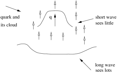
Figure 1: Distribution of the color charge in a cloud.

Figure 2: Running of the couplings from [1].

When the effective coupling becomes weak, one can calculate the screening (or antiscreening) behavior in perturbation theory. In QCD one finds for the change in effective coupling

$${dg(\epsilon)\over d\ln\epsilon}~{}=~{}\beta_{0}g^{3}+\beta_{1}g^{5}+...$$ (8)

with

$$\beta_{0}~{} = ~{}{-1\over 16\pi^{2}}(11-{2\over 3}f)$$ (9)

$$\beta_{1}~{} = ~{}({1\over 16\pi^{2}})^{2}(102-{38\over 3}f),$$ (10)

where $\epsilon$ is the energy, or equivalently inverse length, scale at which the effective charge is defined. Thus if the $f\leq 16$ the effective coupling decreases to zero as the energy at which it is measured increases to infinity, which is asymptotic freedom. Taking the first term only, we see that the asymptotic behavior is approximately

$${1\over g(\epsilon)^{2}}~{}=~{}{1\over g(1)^{2}}-\beta_{0}\ln\epsilon.$$ (11)

2.2.2 Clouds, Jets, and Experiments

The asymptotic freedom of QCD can be exploited to simplify the calculation of many physical processes. To understand why that is so, consider the picture of quarks (or gluons) that it suggests. This is shown in Figure 1. The effective color charge of a quark, responsible for its strong interaction, accumulates over distance. We should think of it as a distributed cloud of induced color charge, all of the same sign, with no singular core. Now consider how this cloud is seen when probed at various wavelengths. If the wavelength is small, the effective color charge will be small, since only a small portion of the cloud is sampled. If the wavelength is large, the effective charge will be large.

One can also consider the complementary particle picture. If one suddenly imparts a large impulse to a quark (or gluon), liberating it from its cloud, the resulting object will have a small effective color charge, and will propagate almost freely, until it builds up a new cloud.

Of course the electric and weak charges of a quark are not shared by its color polarization cloud. These charges remain concentrated. Thus short-wavelength electromagnetic or weak probes can resolve pointlike quarks, whose ‘strong’ (color) interactions make only small corrections to free-particle propagation. More precisely, it is corrections that substantially change the energy-momentum of the color current which are guaranteed to be small. Big changes in the energy-momentum can only arise from radiation of gluons having short wavelength in the frame of the current, but such short-wavelength gluons see only a small effective color charge, as we’ve discussed.

So in physical process originating with the pointlike quarks directly produced by hard electroweak currents, as for instance in $e^{+}e^{-}$ annihilation at high energy, one develops jets of rapidly-moving hadrons following the nominal paths of the original quarks. Hard gluon radiation processes do occasionally occur, of course, but at a small rate, calculable in perturbation theory. These hard gluons can (with small probability) induce jets of their own, which themselves occasionally radiate, and so forth. The “antenna pattern” of jets – including the relative probabilities for different topologies (numbers of jets), the energy and angular distributions for a given topology, and how all these quantities depend upon the total energy, can be calculated in exquisite detail. These predictions, which reflect in 1-1 fashion the structure of the fundamental interactions in the theory and the running of the coupling, have been extensively, and successfully, tested experimentally.

The science of exploiting asymptotic freedom to predict rates for a wide variety of hard processes is highly developed. Figure 2 displays results of comparisons between prediction and observation for a wide variety of experiments, in the form of determinations of the running coupling. Implicit, of course, is that within any given type of experiment, the theory gives a successful account of the functional form of dependence on event topology, energy distribution, angular distribution, … . The Figure itself demonstrates the success of Eqns. 8,9, suitably generalized to include the effect of quark masses, as a description of Nature.

2.2.3 Dimensional Transmutation and “Its From Bits”

Running of the coupling manifestly breaks the classical scale invariance ${\cal R}^{+}_{\rm scale}$. It is an almost inevitable result of quantum field theory. Indeed, quantum field theory predicts as its first consequence the existence of a space-filling medium of virtual particles, whose polarization makes the effective coupling strength depend on the distance at which it is measured, or in other words causes the coupling to run. (There are very special classes of supersymmetric theories in which different types of virtual particles give cancelling effects, and the coupling does not run.)

Because its coupling runs, in QCD the analogue of Pauli’s question:

“Why is the value of the fine structure constant what it is?” –

receives a startling answer:

“It’s anything you like – at some scale or other.”

We can simply declare it to be, say, ${1\over 10}$, thereby defining the correct distance at which to measure it – i.e., the distance where it is ${1\over 10}$! This is the phenomenon of dimensional transmutation. A dimensionless coupling constant has been transmuted into a length (or, equivalently, energy) scale.

In fact we can identify a scale explicitly, using Eqn. 8:

$$M~{}=~{}\lim_{\epsilon\rightarrow\infty}\epsilon e^{u\over\beta_{0}}u^{\beta_{1}\over\beta_{0}^{2}}$$ (12)

where

$$u~{}\equiv~{}{1\over g(\epsilon)^{2}}~{}.$$ (13)

The form of Eqn. 8 insures that the limit exists and is finite.

Due to its formal scale invariance, QCD with massless quarks appears naively – that is, classically – to be a on-parameter family of theories, distinguished from one another by the value of the coupling $g$. And none of these theories, it appears, defines a scale of distance. Through the magic of dimensional transmutation, QCD turns out instead to be a family of perfectly identical clones, each of which does define a distance scale. Indeed, the clones differ only in the units they employ to measure distance. This difference in units enters into comparisons of purely QCD quantities to quantities outside of QCD, such as the ratio of the proton mass to the electron mass. But it does not affect dimensionless quantities within QCD itself, such as ratios of hadronic masses or of isomer splittings.

Using $\hbar$ and $c$ as units, and no further inputs the truncated version of QCD including just the $u$ and $d$ quarks, with their masses set to zero – what I call “QCD Lite” – accounts pretty accurately for the low-lying spectrum of non-strange hadrons (demonstrably), nuclear physics (presumably), and much else besides. The only numerical inputs to QCD Lite are the number of colors – 3 (binary 11) – and the number of quarks –2 (binary 10). Thus QCD Lite provides a remarkable realization of Wheeler’s slogan “Getting Its From Bits”!

2.2.4 Limitations

The most straightforward applications of asymptotic freedom are to processes involving large energy scales only. This constraint pretty much limits one to inclusive processes induced by electroweak currents. Any external hadron introduces a small energy scale, namely its mass. By using clever tricks to isolate calculable subprocesses, one can calculate much more, as conveyed in Figure 2. However these tricks will take you only so far, and there is no easy way to exploit the small effective coupling at short distances to address truly low-energy phenomena, or to calculate the spectrum. If you try to calculate such things directly, you will encounter infrared divergences – so at least the theory is kind enough to warn you off. Similarly, large temperature or large chemical potential introduce large “typical” energies, but it is not trivial (and usually not even true) that this fact in itself will allow access, via asymptotic freedom, to interesting spectral or transport properties.

2.3 Confinement

2.3.1 Brute Facts and Crude Theory

An aura of mystery still seems to hover around the phenomenon of quark confinement. Historically, of course, it was a big surprise in world-modeling, and posed a major barrier both to the discovery and to the acceptance first of quarks, and then of modern QCD. And confinement is a genuinely profound and subtle dynamical phenomenon, as some of our later considerations will emphasize. Concerning the fact that QCD predicts confinement, however, there is no ambiguity. Our knowledge of the properties of the theory has moved far beyond abstract or hypothetical discussion of this point. Figure 3 exhibits the results of some direct calculations of the spectrum starting from the microscopic theory, with controlled errors, using the techniques of lattice gauge theory. There are neither massless flavor-singlet particles with long-range interactions, particles with quark or gluon quantum numbers, nor degenerate color multiplets. In fact the microscopic theory reproduces the observed spectrum extremely well, with no gratuitous additions.

Thus confinement is not a practical problem for modern QCD. Still, one would like to understand more precisely what it is, why it occurs and, particularly for these lectures, whether in can come undone in extreme conditions.

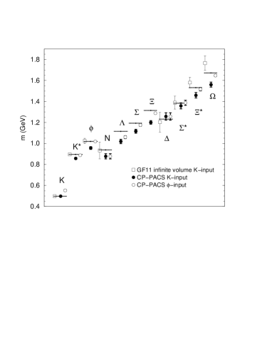
Figure 3: Spectrum from lattice gauge theory, from [2].

The simplest heuristic argument for confinement is due to Amati and Testa. It is based directly on Eqn. 1. If the coefficient ${1\over g^{2}}$ of the gauge curvature term is taken to zero, then upon varying the action with respect to the gauge potential $A_{\mu}$ we find that the color current vanishes, including its zero component, the color charge density – which is to say, color is confined. We can combine this idea with the running of the coupling, to argue (still more heuristically) that low-frequency modes, associated with large effective couplings, are confined, while high-frequency modes can be dynamically active. This is broadly consistent with the observed behavior in Nature, that quarks and gluons become visible in hard processes, but are not accessible to soft probes.

Unfortunately it is a very singular operation to throw away the highest-derivative terms in any differential equation, because they will always dominate for sufficiently abrupt variation. In high Reynolds number hydrodynamics, one addresses this difficulty with boundary layer theory. In QCD, the only method we know to make the simple Amati-Testa argument the starting point for a systematic approximation is by employing an artful discretization, lattice gauge theory, as I’ll now discuss.

2.3.2 Lattice Gauge Theory Basics

The great virtue of the lattice version of QCD are that it provides an ultraviolet cutoff and that it allows a convenient strong-coupling expansion, while preserving a very large local gauge symmetry. Its drawbacks are that it destroys translation and rotation symmetry, that it has an awkward weak-coupling expansion, and that it mutilates the ultraviolet behavior of the continuum theory. But let’s put these worries aside for the moment, and exploit the virtues. Also let’s consider the pure glue theory. The extension to quarks will appear in Lecture 2.

The fundamental operation in gauge theory is parallel transport. The basic objects of the theory are 3$\times$3 unitary matrices with unit determinant. They live on the oriented links of a cubic hyperlattice in four dimensions, and implement parallel transport. Thus the dynamical variable $U_{r,\hat{\mu}}$ is a matrix associated with the link starting from lattice point $r$ and ending at $r+\hat{\mu}a$, where $a$ is the lattice spacing. The matrix associated with the same link oriented in the opposite direction is the inverse, i.e. $U_{r+\hat{\mu}a,-\mu}~{}=~{}U_{r,\hat{\mu}}^{-1}$.

If there were an underlying continuum gauge potential $A$, the parallel transport would be

$$U_{r,\hat{\mu}}~{}\hbox{``}=\hbox{''}~{}\bar{P}\exp i\int^{r+\hat{\mu}a}_{r}A_{\mu}dx^{\mu}~{},$$ (14)

where $\bar{P}$ denotes anti-path ordering. Indeed, this is the solution of the equation

$$\nabla_{\mu}U~{}\equiv~{}(\partial_{\mu}+iA_{\mu})U~{}=~{}0$$ (15)

having the indicated endpoints. In line with this underlying structure, which we would like to recover in an appropriate limit, local gauge transformations $\Omega(r)$ should act on the lattice sites, and transform the $U$ matrices according to

$${\tilde{U}}_{r,\mu}~{}=~{}\Omega(r)U_{r,\mu}\Omega(r+\hat{\mu}a)^{-1}~{}.$$ (16)

The $\Omega(r)$ are, of course, 3$\times$3 unitary matrices.

To form interaction terms invariant under Eqn. 16 one must take the trace of a product of $U$ matrices along a path of links forming a closed loop. The simplest possibility is simply the trace around a plaquette, e.g.

$${\rm tr}~{}{\it Pl}_{r,\hat{x}\hat{y}}~{}\equiv~{}{\rm tr}~{}U_{r,\hat{x}}U_{r+a\hat{x},\hat{y}}U_{r+a\hat{x}+a\hat{y},-\hat{x}}U_{r+a\hat{y},-\hat{y}}~{}.$$ (17)

Putting Eqn. 14 into Eqn. 17 and expanding for small $a$, we find the first non-trivial term

$${\rm tr}~{}{\it Pl}_{r,\hat{x}\hat{y}}~{}\rightarrow{\rm tr}~{}(1-{a^{4}\over 2}G^{xy}G_{xy})+O(a^{6})~{}.$$ (18)

The straightforward verification of Eqn. 18 is quite arduous, but one can restrict its form a priori by exploiting gauge invariance, and then evaluate on a simple configuration such as $A_{x}~{}=~{}M(y-r_{y})$. Note that a term $\propto a^{2}G^{xy}$, which does appear in the plaquette product, vanishes when we take the trace.

Thus the simplest lattice gauge invariant action we can write, the Wilson action

$$S_{W}~{}=~{}{1\over 4g^{2}}\sum_{\rm plaquettes}(3-{\rm tr}~{}{\it Pl}_{\Box})~{}~{}$$ (19)

reduces, formally, to the continuum action for very small lattice spacings. Hence we are invited to use it, and then attempt to justify the limit. (In the spirit of the Jesuit credo “It is more blessed to ask forgiveness than permission.”)

To evaluate a correlation function of operators $\langle{\cal O}_{1}{\cal O}_{2}...\rangle$, then, we must evaluate the integral

$${\langle{\cal O}_{1}{\cal O}_{2}...\rangle~{}=~{}\int d{\cal M}\exp(-S_{W}){\cal O}_{1}{\cal O}_{2}...\over\int d{\cal M}\exp(-S_{W})}~{},$$ (20)

where

$$d{\cal M}~{}=~{}{\textstyle\prod}_{{\rm links}~{}r,\hat{\mu}}U_{r,\hat{\mu}}^{-1}dU_{r,\hat{\mu}}$$ (21)

is the product of invariant integrals over the gauge group.

2.3.3 Strong Coupling and Confinement

The lattice regularization permits one to formulate strong coupling perturbation theory in a simple, elegant way. When $g$ gets large, we can simply expand $e^{-S_{W}}$ in a power series in ${1\over g^{2}}$. The result is to “bring down” activated plaquettes, one for each inverse power of ${1\over g^{2}}$. When we integrate over a link incident on an activated plaquette, we encounter an extra power of $U$ for that link.

To test for confinement, the traditional method is to study Wilson-Polyakov loops. These are simply the traces of products of $U$ matrices around loops, similar to the terms that appear in the action. But now we want to consider large loops, instead of very small ones.

The motivation for this method is as follows. Suppose we put a very heavy quark into the system. This will stay at a fixed point in space, so its world-line will be simply a straight line in the $\hat{\tau}$ (Euclidian time) direction. The ${\rm tr}~{}j\cdot A$ coupling of this color source will generate a product of $U$ matrices along the links of its world-line. So to measure the potential between a heavy quark and a heavy antiquark at distance $R$ we should measure the energy it takes to have a line like this and a similar line with $U^{-1}$ matrices a distance $R$ away. If we allow this configuration to persist for a long Euclidian time $T$, the cost should go as $e^{-V(R)T}$. Now to make the “measurement” clean we should imagine closing up the loop with short segments at the top and bottom. This corresponds to producing the quark-antiquark pair, letting them sit separated for a long time, and then annihilating them. With $R<<T$, by taking the negative of the log, we will extract the potential. In a formula

$$V(R)~{}=~{}\lim_{T\rightarrow\infty}{-1\over T}\ln{\int d{\cal M}\exp(-S_{W})\Pi\over\int d{\cal M}\exp(-S_{W})}~{}.$$ (22)

where $\Pi$ is the trace of an ordered product of $U$ matrices along the perimeter of a long rectangle with sides of length $R$ and $T$, as shown in Figure 4a.

Figure 4: (a) The Wilson loop: insertion of a color (unit triality) source.

With this background in hand, it becomes very easy to understand how confinement arises in strong coupling. The integral of a single $U$ matrix over the group manifold, $\int U^{-1}dUU$, vanishes. (The change of variables $U\rightarrow gU$ leaves the measure invariant, so if $\int U^{-1}dUU=k$, then by changing variables we find $gk=k$ for any $g$, which of course means $k=0$.) So does $\int U^{-1}dUU^{-1}$. Thus to find a non-zero contribution to Eqn. 22 in strong coupling we must at least pull down plaquettes to share sides with each of the links in the Wilson loop.

Figure 4: (b) Tiling of Wilson Loop in strong coupling.

But now you see there’s a whole new set of interior links with single $U$ matrices and vanishing group integrals. Clearly, to get a non-zero contribution we must tile the whole area spanned by the Wilson loop, as in Figure 4b. This takes a number of plaquettes proportional to the area $RT$, at least. So the leading contribution to the Wilson loop in strong coupling goes as

$$V(R)~{}\sim~{}-{1\over T}\ln({1\over g^{2}})^{RT}~{}\propto R~{}.$$ (23)

The linear potential, of course, means that it is impossible to separate the color sources indefinitely, and so one has confinement.

2.3.4 To the Continuum Limit

The strong coupling result forms the starting point for a convincing proof of confinement in (pure glue) QCD proper.

One first argues that the strong coupling perturbation theory has a finite radius of convergence. That can be done analytically. Then one investigates numerically whether there is a phase transition as a function of the coupling, as the coupling varies from strong to weak. It turns out there is a phase transition for $U(1)$, but not for $SU(3)$ (or $SU(2)$). When there is no phase transition, the theory remains in the same universality class, and its sharply defined qualitative properties cannot change.

Thus in the physically relevant $SU(3)$ case:

• Since the strong coupling perturbation expansion converges, the lowest non-trivial order governs the asymptotic behavior of the Wilson loop, and exhibits confinement.

• Since the strong coupling theory is in the same universality class as the weak coupling theory, the weak coupling theory also exhibits confinement.

• Since asymptotic freedom implies that the weak coupling lattice theory reproduces the continuum theory, the continuum theory exhibits confinement.

Now we see that is fortunate, and reassuring for this circle of ideas, that there is a phase transition for $U(1)$. Otherwise we’d have proved confinement in QED, which would be proving too much.

2.3.5 Foundational Remarks

To round out this discussion I would like to emphasize the deep connections among renormalizability, asymptotic freedom, and lattice gauge theory. To construct a relativistic quantum theory, one typically introduces at intermediate stages a cutoff, which spoils the locality or relativistic invariance of the theory. Then one attempts to remove the cutoff, while adjusting the defining parameters, in order to achieve a finite, cutoff-independent limiting theory. Renormalizable theories are those for which this can be done, order by order in a perturbation expansion around free field theory. That formulation of the problem of constructing a quantum field theory, while convenient for mathematical analysis, obviously begs the question whether this perturbation theory converges. For interesting quantum field theories, it rarely does.

A more straightforward procedure, conceptually, is to regulate the theory as a whole by discretizing it. This involves approximating space-time by a lattice, and spoils the continuous space-time symmetries of the theory. Then one attempts to remove dependence on the discretization, by refining it, while if necessary adjusting the defining parameters, to achieve a finite limiting theory that does not depend on the discretization, and therefore has a chance to respect the space-time symmetries. The redefinition of parameters is necessary, because in refining the discretization one is introducing new degrees of freedom. The earlier, coarser theory results from integrating out these degrees of freedom. If it is to represent the same physics it must incorporate their effects, for example in vacuum polarization. Operationally, one can demand that some observable(s) measured at scales well beyond the lattice spacing stays fixed as the discretization is refined. This fixes the free coupling(s). The question is then whether, having fixed the available parameters, the calculated values of all observables have finite limits.

This is very hard to prove, in general. The only case in which it is straightforward arises when the effects of integrating out the additional short-wavelength modes, that are introduced with each refinement of the lattice, can be captured accurately by a re-definition of the coupling parameter(s) already present in the theory. That, in turn, will occur in a straightforward way only if these modes are weakly coupled. For then perturbation theory will show us how to take the limit for the renormalizable couplings, while assuring us that naive power counting can be applied to argue away all non-renormalizable ones. But of course the ultraviolet modes will be weakly coupled, if and only if the theory is asymptotically free.

Summarizing the argument, only those relativistic field theories which are asymptotically free can be argued in a straightforward way to exist. Furthermore, the only asymptotically free theories in four space-time dimensions involve nonabelian gauge symmetry, with highly restricted matter content. So the axioms of gauge symmetry and renormalizability which we invoked to define QCD are, in a certain sense, redundant. They are implicit in the mere existence of non-trivial interacting quantum field theories.

Figure 4: (c) Perimeter law, in the theory with quarks.

2.4 Chiral Symmetry Breaking

2.4.1 Numerical and Laboratory Phenomena

The most direct evidence for chiral symmetry breaking in QCD comes form numerical simulation of the theory. One simply computes the expectation value

$$\langle{\bar{q_{L}}}_{i}{q_{R}^{j}}\rangle\propto v\delta^{j}_{i}\neq 0$$ (24)

in the ground state for the theory with massless quarks. This condensation, which breaks the chiral symmetry of the equations, is entirely analogous to the development of spontaneous magnetization in a ferromagnet. As in that case, for any finite sample (e.g., in any simulation) we must add an infinitesimal biasing field to stabilize a particular alignment.

In Eqn. 24 I’ve chosen to align in the flavor diagonal direction, but in the absence of a biasing field any chirally rotated configuration, with $q_{R}\rightarrow Uq_{R}$, will have the same energy but $\delta^{i}_{j}\rightarrow U^{i}_{j}$ in the expectation value, for any $U\epsilon SU(f)$. There are several technical issues in the simulations that arise and must be addressed, but the numerical evidence that chiral symmetry is spontaneously broken is unambiguous and overwhelming, at least for $2\leq f\leq 4$. I’ll discuss this evidence in more detail in Lecture 2.

The historical path whereby spontaneous chiral symmetry was discovered as a property of Nature was of course quite different. Indeed, the discovery of chiral symmetry breaking in the strong interaction antedates by more than a decade the discovery of QCD as its microscopic theory.

The conceptual starting point for the historic development was the observation, coming into focus with the BCS theory of superconductivity, that if a symmetry is spontaneously broken there will be massless collective modes associated with this breakdown. (The “experimental” starting point was the Goldberger-Treiman relation; see below.) Quite generally, suppose the ground state of a physical system (e.g. a ferromagnet or the no-particle state of QCD at zero temperature) is characterized by the existence of a condensate

$$\langle\eta|{\cal M}^{a}_{b}|\eta\rangle=\eta^{a}_{b}$$ (25)

that violates a continuous symmetry of the underlying equations (e.g. rotational or chiral symmetry, respectively). Let the symmetry $g$ of the underlying theory be implemented by the unitary operator $U(g)$, with $U(g)^{-1}MU(g)=\rho(g)M$. Then if $\rho(g)\eta\neq\eta$, which is the signature of symmetry breaking, the states

$$U(g)|\eta\rangle~{}\equiv~{}|\rho(g)\eta\rangle$$ (26)

will be physically distinct from the ground state, but energetically degenerate with it. By moving slowly within this manifold of states, as a function of space, we would expect to create states whose energy goes to zero as the wavelength of the variation goes to infinity. In a particle interpretation, the quanta of the field that creates such configurations will be massless. Furthermore, we have constructed a very specific realization of these quanta in terms of symmetry generators. This construction can be exploited to yield predictions for their properties. For example, if the broken symmetry is an internal symmetry, the quanta will be spin-0 particles.

Turning now specifically to the world of strong interactions, it is a striking fact that $\pi$ mesons are spin-0 particles which are much lighter than all other hadrons. This suggests the possibility that they are associated with the spontaneous breakdown of an approximate internal symmetry. Their pseudoscalar character, and the fact that they form an isotriplet, suggests the breaking pattern

$$SU(2)_{L}\times SU(2)_{R}~{}\rightarrow SU(2)_{L+R}~{}.$$ (27)

This very specific picture of pions as collective modes closely connected to broken chiral symmetry, besides explaining their quantum numbers and small mass, can be exploited to give many predictions about their low-energy behavior, as we shall discuss in Lecture 2. The phenomenological success of these predictions validates the hypothesis of spontaneously broken approximate chiral symmetry as a description of Nature.

Within QCD, this picture arises very naturally. If the $u$ and $d$ masses are small the basic equations of QCD will exhibit approximate chiral symmetry. And numerical work QCD spontaneously develops a symmetry-breaking condensate, as I mentioned. The general theoretical machinery for extracting predictions from spontaneous symmetry breaking remains valid and extremely valuable in modern QCD. Additionally, the specific form of intrinsic breaking in QCD, through small quark mass terms, has specific phenomenological consequences. I will spell out how all this works below in Lecture 2, when we discuss order parameters and effective Lagrangians. As we shall see, all these concepts take on additional twists, and become even more central, for QCD in extreme conditions.

2.4.2 Ironic Aside

Ironically, the first generation of developments in high-energy physics to be inspired by modern superconducitivity theory were inspired by BCS pairing theory in the limit that the gauge coupling – that is, electromagnetism, and hence the phenomenon of superconductivity – is neglected. In that limit it is the global symmetry of electron number that is violated by the formation of a Cooper pair condensate, and there is a massless collective mode. Spontaneous breaking of a global symmetry turns out to be the appropriate, and fruitful, idea for chiral symmetry breaking in the strong interaction.

There was an interval of several years before the second generation of developments, when the gauge coupling was reinstated. Only then did the primary phenomenon of superconductivity itself – the Meissner effect – enter the picture. Rechristened in its new context as the Higgs mechanism, it of course became central to modern electroweak interaction theory.

2.4.3 Pairing Heuristics

Just as for confinement, the fact of spontaneous chiral symmetry breaking in QCD is no longer negotiable. Still, just as for confinement, one would like to understand why and how it occurs, and whether there are circumstances in which it can come undone.

A heuristic model for chiral symmetry breaking was supplied by Nambu and Jona-Lasinio long before modern QCD. Amazingly, with some re-labeling of the players the concepts they introduced still apply. Indeed, as we shall see, at high density they come to look better than ever. We shall be discussing pairing theory in great detail in Lecture 4, so this is just a foretaste.

Suppose one has an attractive four-fermion interaction

$${\cal L}_{\rm int.}~{}=~{}g(\bar{\psi}\psi)(\bar{\psi}\psi)~{}.$$ (28)

Then one can imagine that it is energetically favorable to form a condensate

$$\langle\bar{\psi}\psi\rangle~{}=~{}v\neq 0~{},$$ (29)

since this condensate generates negative interaction energy. Indeed, if the condensate is so large that we can ignore quantum fluctuations, we shall have the condensation energy density

$$\Delta{\cal E}~{}=~{}-\Delta{\cal L}~{}=~{}-g\langle\bar{\psi}\psi\rangle^{2}$$ (30)

To test this idea in the simplest crude way, write

$$(\bar{\psi}\psi)^{2}~{}=~{}(\bar{\psi}\psi-v)^{2}+2v\bar{\psi}\psi-v^{2}$$ (31)

and, in the interaction Lagrangian, discard the fluctuating first term (as is approximately valid at weak coupling). The other terms, when added to the standard kinetic energy term for massless fermions, generate the Lagrangian for free massive fermions. One can of course diagonalize this quadratic approximate Lagrangian and, by filling the negative energy sea, construct the appropriate zero fermion number density ground state (i.e., for a given value of the condensate). Then one can enforce consistency by calculating $\langle\bar{\psi}\psi\rangle$ in this state, and demanding that it is equal to the originally assumed value $v$. This consistency equation is called the gap equation, in honor of its ancestor in BCS theory. If the gap equation has a non-trivial solution, one will have lowered the energy by forming a condensate.

In QCD, the one-gluon exchange interaction is quite attractive in the quark-antiquark color singlet channel. This is hardly surprising, since by forming a singlet one cancels the charge and eliminates field energy. To make a scalar condensate in this channel, one must pair left-handed antiquarks with right-handed quarks. So there are simple heuristic reasons to anticipate the possibility of spontaneous chiral symmetry breaking in QCD.

Figure 5: Pairing picture for chiral symmetry breaking. The dots indicate the position of modes that pair. In the limit of zero energy, you must go the the tip of the light cone.

Whether spontaneous chiral symmetry breaking actually occurs, however, is a delicate question, because it involves a competition. The interaction energy one gains by pairing up occupied particle and antiparticle modes must compete against the kinetic energy lost in occupying them. The kinetic energy can become arbitrarily small, but only for a density of states that likewise vanishes – the tip of the Lorentz cone as shown in Figure 5. So whether the interaction energy ever wins out, or not, is a delicate dynamical issue. For example, there is some evidence that as the number of flavors $f$ grows the strength of chiral condensation (relative the the primary QCD scale) shrinks, and that for large enough $f$ (6? 7?) it’s gone. This comes about, presumably, because for larger $f$ the effective coupling does not run so quickly to large values at small energy.

It’s quite a different story at high density. In that case the density of states does not vanish, and spontaneous chiral symmetry breaking can appear at arbitrarily weak coupling, where we have excellent analytic control.

2.5 Chiral Anomalies and Instantons

2.5.1 The Historic Case

The original discovery of the chiral anomaly involved what in hindsight is a fairly complicated example of the phenomenon. It came about not through abstract investigation of mathematical models, but in the process of analyzing a very specific physical process, the decay $\pi^{0}\rightarrow\gamma\gamma$. This is obviously an electromagnetic decay, so to treat it we must consider QCD coupled to QED. The combined theory, though it violates isospin, still appears to be invariant under axial $I_{3}$ symmetry. (I will work, for simplicity, in the limit of vanishing $u$ and $d$ quark masses. This can be shown to be a good approximation for estimating the $\pi\gamma\gamma$ vertex, though of course the actual $\pi^{0}$ mass must be inserted when we use this amplitude to calculate the decay rate.) If this were true, then the $\pi^{0}$ would still be accurately a collective Nambu-Goldstone mode associated with the spontaneous breaking of axial $I_{3}$ symmetry. The coupling $\pi^{0}F^{\mu\nu}{\tilde{F}}_{\mu\nu}$ would be forbidden, because at long wavelength such a Nambu-Goldstone mode is derivatively coupled to the corresponding current. Of course one can rewrite $\pi^{0}F^{\mu\nu}{\tilde{F}}_{\mu\nu}\rightarrow{1\over 2}\partial^{\mu}\pi^{0}A^{\nu}{\tilde{F}}_{\mu\nu}$ inside the Lagrangian, after an integration by parts. However the electromagnetic term is not part of the axial $I_{3}$ symmetry current, classically.

The brilliant result of Adler, Bell and Jackiw is that when one investigates the situation more deeply, using the full resources of quantum field theory, such a term does in fact occur. (Again, the original analysis antedates QCD, and therefore was couched in rather different language. Its details are fascinating and of considerable historical interest, but I will not discuss them here.) Moreover its coefficient can, given an underlying theory of the strong interaction, be calculated precisely. When the coefficient is calculated in a free quark model – with colored, fractionally charged quarks – one finds agreement between the predicted rate for $\pi^{0}\rightarrow\gamma\gamma$ and experiment. Remarkably, the free-quark result remains valid in QCD.

The mechanism whereby the extra term is generated is quite subtle. It is most readily seen in perturbation theory, though a non-perturbative derivation is possible.

Figure 6: Triangle graph, crucial for anomalies and Higgs particle phenomenology.

To regulate the triangle graph and other loop graphs with circulating fermions it is convenient to follow the procedure of Pauli and Villars. In this procedure, one introduces into the theory fictitious boson fields $\phi$ carrying all the same quantum numbers as the fermions (including spin ${1\over 2}$, and so flouting the spin-statistics theorem) but having a large mass $M$. Since the boson loops differ in sign from the fermion loops their contributions will cancel at very large virtual momentum, where the divergences arose. Thus one achieves finite integrals. Then one takes the limit $M\rightarrow\infty$, fixing a few low-energy amplitudes by setting them equal to their physical values. The basic result of renormalization theory is that in suitable (renormalizable) quantum field theories, having used a small number of low-energy amplitudes, to determine the couplings – which will be functions of the cutoff and a few physically determined parameters – all remaining physical amplitudes will approach a finite limit, order by order in perturbation theory. Of course the limiting amplitudes no longer contain contributions arising from the fictitious bosons as intermediate states, because those particles have been driven to infinite mass.

This is not the place to review the technicalities of renormalization theory. Fortunately, for present purposes we don’t need their details. Our focus is simply the triangle graph for the two-photon matrix element of the divergence of the axial current. This graph, by naive power counting, is linearly convergent in the ultraviolet by power counting. In more detail, there are three fermion propagators, and gauge invariance pulls out two powers of momentum to make $F$s from $A$s. However, one will only be able to use gauge invariance if one has employed a gauge invariant regulator, like Pauli-Villars.

By the same power counting, the leading $M$ dependence of the regulated integral, which arises from the Pauli-Villars boson loop, goes as ${1\over M}$ for large $M$. This might seem to make it negligible. The large mass $M$, however, involves a large violation of chiral symmetry. Specifically, it implies a large coefficient $\propto M$ in the divergence of the axial current:

$$\partial_{\mu}(\bar{\phi}\gamma^{\mu}\gamma^{5}\phi)~{}=~{}2M\bar{\phi}\gamma^{5}\phi~{}.$$ (32)

(To have a regulated chiral symmetry that will behave sensibly as we remove the cutoff, the Pauli-Villars fields must transform in the same way as the quark fields they regulate.) This factor exactly cancels the convergence factor, leaving a finite residual contribution. The regulator, necessary to control the contribution of highly virtual quarks, spoils naive chiral symmetry. That is the essential mechanism of the chiral anomaly.

2.5.2 An Easier Version

The basic mechanism leading to anomalies is nicely illustrated, in a context where it is relatively easy to understand, by the process $h\rightarrow GG$ of Higgs particle decay into two gluons. Since this process is of independent and timely interest, I hope you’ll forgive a brief diversion.

The coupling of the standard model Higgs boson to quarks is given as

$${\cal L}_{\rm int}~{}=~{}-2^{1\over 4}G_{F}^{1\over 2}h\sum m_{i}{\bar{q}}_{i}q_{i}~{},$$ (33)

where $G_{F}$ is the Fermi coupling constant. The direct coupling to ordinary matter would seem to be extremely feeble, due to the very small masses of the $u$ and $d$ quarks. Ordinarily one would expect that the contribution from the heavy quarks would be suppressed, according to general “decoupling” theorems. Indeed, we’d be in pretty bad shape in physics if we always had to worry about big contributions to low-energy amplitudes from (potentially unknown) heavy particles. However there is an exception of sorts here, because the coupling grows with the mass. Thus the contribution to the dimension 5 induced interaction term

$${\cal L}_{\rm induced}~{}=~{}\kappa h~{}{\rm tr}~{}G^{\mu\nu}G_{\mu\nu}$$ (34)

arising through a heavy quark loop of circulating heavy quarks in the triangle graph of Figure 6, which by power counting one might expect to be inversely proportional to the mass of the quark, is instead unsuppressed. (Of course, this time the external legs are a Higgs particle and two gluons.) This is very similar to what we saw for the triangle anomaly, but now with real heavy particles rather than virtual regulators. One finds

$$\kappa~{}=~{}2^{1\over 4}G_{F}^{1\over 2}{g^{2}\over 48\pi^{2}}$$ (35)

per heavy quark, in the large mass limit ($m_{h}\mathrel{\raise 1.29167pt\hbox{$<$}\mkern-14.0mu\lower 2.58334pt\hbox{$\sim$}}m_{q}$). For values $90~{}{\rm Gev}\mathrel{\raise 1.29167pt\hbox{$<$}\mkern-14.0mu\lower 2.58334pt\hbox{$\sim$}}m_{h}\mathrel{\raise 1.29167pt\hbox{$<$}\mkern-14.0mu\lower 2.58334pt\hbox{$\sim$}}150~{}{\rm Gev}$ of the Higgs mass most interesting for ongoing searches this “anomalous” gluon coupling generates both the dominant mechanism for hadronic production of $h$ particles, and a significant decay mode for them.

2.5.3 The Saga of Axial Baryon Number

For concreteness in this part I’ll mostly take $f=2$ and refer to the quarks as $u$ and $d$. This simplifies the notation, loses nothing essential, and is close to reality.

The spontaneous breakdown of approximate chiral $SU(2)_{L}\times SU(2)_{R}\rightarrow SU(2)_{L+R}$ is associated with an extensive, successful phenomenology. At the level of quarks in QCD, we understand it as the result of the development of a condensate $\langle\bar{u_{L}}u_{R}\rangle~{}=~{}\langle\bar{d_{L}}d_{R}\rangle$. This condensate also violates the axial baryon number symmetry under $(u_{L},d_{L})\rightarrow e^{i\alpha}(u_{L},d_{L})$, $(u_{R},d_{R})\rightarrow e^{-i\alpha}(u_{R},d_{R})$, which is a symmetry of Eqn. 1. One might expect, then, a light Nambu-Goldstone boson with the associated properties – a light, flavor-singlet pseudoscalar with highly constrained couplings. Alas, there is no such particle. Thereby hangs a tale.

The first observation is that there is an “anomalous” contribution to the divergence of the axial baryon number current, arising from the triangle graph of Figure 6. There’s a new set of players – the axial baryon current instead of axial $I_{3}$, and gluons instead of photons – but they follow the same script. Thus we find

$$\partial_{\mu}j_{B}^{\mu 5}~{}\equiv~{}\partial_{\mu}(\bar{u}\gamma^{\mu}\gamma^{5}u+\bar{d}\gamma^{\mu}\gamma^{5}d)~{}=~{}{g^{2}\over 4\pi^{2}}{\rm tr}~{}{\tilde{G}}_{\mu\nu}G^{\mu\nu}~{},$$ (36)

where ${\tilde{G}}_{\mu\nu}\equiv{1\over 2}\epsilon_{\mu\nu\alpha\beta}G^{\alpha\beta}$ is the dual field strength. The current $j_{B}^{\mu 5}$ is not conserved. Naive axial baryon number symmetry, generated by the spatial integral of $j_{B}^{05}$, is spoiled by an anomaly.

However, the existence of this anomaly does not in itself remove the problematic mode. For one has

$${\rm tr}~{}G^{\mu\nu}{\tilde{G}}_{\mu\nu}~{}=~{}\partial_{\mu}K^{\mu}$$ (37)

where

$$K_{\mu}~{}=~{}{1\over 2}\epsilon_{\mu\alpha\beta\gamma}{\rm tr}~{}(A^{\alpha}\partial^{\beta}A^{\gamma}+{2\over 3}A^{\alpha}A^{\beta}A^{\gamma})~{}.$$ (38)

Thus it would appear that a modified symmetry, generated by the charge associated with the modified conserved current $j^{A5}_{\mu}-K_{\mu}$, is spontaneously broken, leaving us not much better off than before, still with the mistaken prediction of an extra light flavor singlet pseudoscalar.

Fortunately, though, Eqn. 37 is itself problematic. The point is that $K_{\mu}$ is a gauge-dependent quantity, so that in principle it can be singular without implying the singularity of any physical observable.

We can be more specific about this in the context of a path integral treatment of the theory. In such a treatment we express quantum amplitudes as an integral of contributions from different classical field configurations. To have reasonable control of the functional integrals – to have a measure that is damped for large field strengths – we must consider the Euclidian form of the theory, rotating to imaginary values of the time. In this framework, consider the behavior of the gauge potentials $A_{\mu}$ at spatial infinity. For the integral of $K_{\mu}$ to acquire a non-vanishing surface term, and thereby violate the formal conservation law, requires that $A_{\mu}(x)\sim{M_{\mu}(\hat{x})\over|x|}$. This is not allowed for generic forms of $M_{\mu}(\hat{x})$, since a non-trivial field strength $G\sim{1\over r^{2}}$ would result, leading to a logarithmically divergent action. But for special values of the boundary conditions $M_{\mu}(\hat{x})$ these can cancel, leaving behind a finite-action contribution to the functional integral that contributes to $\partial_{\mu}K^{\mu}$.

In the weak-coupling limit, we look for the field configurations that contribute to the amplitude of interest that have the smallest possible action. For amplitudes that violate axial baryon number (non-vanishing $\int G^{\mu\nu}\tilde{G}_{\mu\nu}$) these configurations are instantons, much-studied classical solutions of the Euclidian Yang-Mills equations.

A very important consistency check is that the integral $\int{\rm tr}~{}G^{\mu\nu}\tilde{G}_{\mu\nu}$, which according to the anomaly equation measure the violation of axial baryon number, must turn out to be quantized (that is, come in discrete units – it’s a c-number integral). Indeed, since axial baryon number is quantized, changes in axial baryon number had also better be quantized. The facts we have discussed, that this integral can be thrown onto the surface at infinity and that its finiteness requires special conspiracies, suggest a connection to topology and the possibility of its quantization. These features can indeed be demonstrated, but I won’t do that here.

In view of the easily proved inequality

$$\int{\rm tr}~{}G^{\mu\nu}G_{\mu\nu}\geq|\int{\rm tr}~{}G^{\mu\nu}\tilde{G}_{\mu\nu}|$$ (39)

quantization of the right-hand side implies that the action of any configuration leading to axial baryon number violation is bounded below by a finite constant. Thus in the function integral such configurations are suppressed by a factor $e^{-{1\over g^{2}}{\rm const.}}$. In particular, they vanish to all orders in perturbation theory!

Instantons violate axial baryon number, but none of the other chiral flavor symmetries. This allows us to visualize their effect quite simply, at a heuristic level. The flavor structure must contain a product of determinant factors

$${\cal L}_{\rm inst.}~{}\propto~{}\epsilon_{ij}q_{L}^{i}q_{L}^{j}\epsilon^{kl}\bar{q_{R}}_{k}\bar{q_{R}}_{l}~{}.$$ (40)

For $f$ flavors, we’d have $f$ lefties in and $f$ righties out. The structure of the color and spin indices, and the form-factor accompanying this interaction, are more tricky to work out. To do it one must solve for the fermion zero-modes in the presence of an instanton. The resulting effective non-local “‘tHooft interaction” is represented pictorially in Figure 7: lots of fermions emerging from an extended gluon cloud.

Figure 7: ‘tHooft interaction. Chirality is violated by a knot of gluon energy.

Unfortunately, for reasons we have discussed before, the formal weak-coupling limit that leads us to focus on instantons is not under control for QCD in vacuum. So the arguments used in this section, while certainly suggestive, cannot be made quantitative in a convincing way. (Nevertheless, some reasonably successful phenomenology has been done by the saturation of the functional integral by superpositions of instantons and anti-instantons as a starting point.) Remarkably, under extreme conditions the theoretical situation for axial $U_{A}(1)$ breaking comes under much better control, with interesting consequences, as we’ll see.

3 Lecture 2: High Temperature QCD: Asymptotic Properties

3.1 Significance of High Temperature QCD

In this lecture I shall be discussing the behavior of QCD (and some closely related models) at high temperature and zero baryon number density. Since that is a mouthful I’ll just say high temperature.

The high temperature phase of QCD is of interest from many points of view. First of all, it is the answer to a fundamental question of obvious intrinsic interest: What happens to empty space, if you keep adding heat? Moreover, the high density phase of QCD was (almost certainly) the dominant form of matter during the earliest moments of the Big Bang. Moreover, it is a state of matter one can hope to approximate, and study systematically, in heavy ion collisions. Major efforts are being directed toward this goal and significant, encouraging results have already emerged. One can also simulate many aspects of the behavior with great flexibility and control, from first principles, using the techniques of lattice gauge theory. One can also make progress analytically. So there is a nice interplay among physical experiments, numerical experiments, and theory.

The fundamental theoretical result regarding the asymptotic high temperature phase is that it becomes quasi-free. That is, one can describe major features of this phase quantitatively by modeling it as a plasma of weakly interacting quarks and gluons. In this sense the fundamental degrees of freedom of the microscopic Lagrangian, ordinarily only indirectly and very fleetingly visible, become manifest (or at least, somewhat less fleetingly visible). Likewise the naive symmetry of the classical theory which, as we saw in Lecture 1, is vastly reduced in the familiar, low-temperature hadronic phase, gets restored asymptotically. In particular, chiral symmetry is restored, and confinement comes completely undone. Axial baryon number and scale symmetry, though never precisely restored, become increasingly accurate.

Since there are dramatic qualitative differences between the zero-temperature and the high-temperature phases, the question naturally arises whether there are sharp phase transitions separating them, and if so what is their nature. This turns out to be a rich and intricate story, whose answer depends in detail on the number of colors and light flavors. In the course of addressing it, we shall have to refine and modify common, rough intuitions about chiral symmetry and (especially) confinement. After an involved but I think interesting and coherent story, building up from the study of various idealizations, we shall find that there is, plausibly, a true phase transition in real QCD that we can converge upon from several directions – experimentally, numerically, and analytically.

3.2 Numerical Indications for Quasi-Free Behavior

For technical reasons it has been difficult until recently to simulate QCD including dynamical quarks with realistically small masses. That situation is changing, but it will be a few years before accurate quantitative results for thermodynamic quantities for QCD with light dynamical quarks become available.

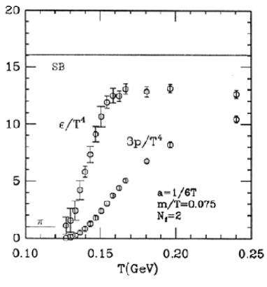
Figure 8: Energy density and pressure of 2-flavor QCD as a function of temperature.

Fortunately, we can already learn a lot from the existing simulations using pure glue or glue plus moderately massive quarks.

Representative results for the temperature dependence of the energy density and pressure in the two flavor theory are shown in Figure 8. Clearly, there is a rapid crossover in the behavior, with dramatic rises in the energy density and pressure (even when normalized to $T^{4}$) over a small range of temperatures around 150 Mev.

A notable feature of the numerical results is that while the energy density (divided by $T^{4}$) ascends rapidly to something close to its asymptotic value, the pressure appears much more sluggish. Thus the behavior of the plasma, even in regard to this basic bulk property, differs significantly from a free gas of massless particles. It is a worthy challenge to compute the corrections to free behavior analytically in weak coupling. This is not entirely straightforward, due to the absence of magnetic screening in perturbation theory (concerning which, more below). For recent progress see [3].

In reality the only hadrons light on the scale of the computed cross-over temperature are pions. Thus for temperatures significantly below this temperature (say $T\leq 120~{}{\rm Mev}$) one has a rather dilute gas of pions, with 3 massive degrees of freedom for the three possible charge states of these spinless particles. Asymptotically, on the other hand, one has a gas with three different flavors of quarks, each of which comes with two spins, three colors, and antiquarks. Also there are eight gluons, each with two helicities. Thus the number of degrees of freedom is $3\times 2\times 3\times 2+8\times 2=52$, of which all but the strange quarks are essentially massless. Evidently, the difference is gigantic! Remarkably, the change from one regime to the other appears to occur largely within a narrow range of temperatures around 150 Mev, amazingly low if regarded from the hadron side.

3.3 Ideas About Quark-Gluon Plasma

The physics of quark-gluon plasma is already a big subject with a vast literature. It will bloom further as the RHIC and ALICE programs gather data. Let me briefly sketch a few of the characteristic phenomena that have been discussed.

• A fundamental foundational result is the observation that distributions of particle energies in the final state are well described by thermal distributions corresponding to a freeze-out temperature around 120 Mev. This observation makes it extremely plausible, as had already been anticipated from theoretical work, that approximate thermal equilibrium (at least, kinetic equilibrium) is established – at higher temperatures, of course – in the initial fireball. That’s very good news, both because it makes the theoretical analysis easier, and because it means that the collisions really are approximating the conditions which are of most fundamental interest.

• The most basic and profound prediction is what I have already mentioned, that one should have approximately the energy and pressure characteristic of the appropriate – large! – number of microscopic degrees of freedom. Qualitatively, this means among other things a steep rise in the specific heat, so that the rise of temperature with energy will slow markedly. Energy will go into particle production, not motion. In principle, the temperature is accessible either through measurement of the transverse momenta of hard leptons or photons emerging from the initial fireball. The entropy can be estimated from the final thermal particle distribution at freezeout, since the expansion and cooling should be roughly adiabatic until freezeout. Several more sophisticated flow diagnostics have been proposed to give handles on the full equation of state.

• Since strange quarks are expected to be much lighter than the lightest hadrons ($K$ mesons) in which they are found, one can anticipate a significant rise in the relative multiplicities of strange (and antistrange) particles, relative to normal hadronic collisions. There is already a striking phenomenon of this kind seen at SPS, with a dramatic rise (as much as a factor 15) in $\Omega$ and $\bar{\Omega}$ production.

• Perhaps the single most striking experimental result to emerge so far from the study of heavy ion collisions is the suppression of J/$\psi$, relative to Drell-Yan background, in lead-lead collisions at the highest energies. When the ratio is plotted as a function of atomic weight and energy, a clear break in its behavior, relative to lower energies or lower atomic numbers, leaps to the eye. No hadron-based model of the collision process anticipated this break, and none has been successful in reproducing it. On the other hand an effect of just this sort was anticipated, based on simple qualitative arguments, to mark the onset of quark-gluon plasma behavior.

  The basic point is that free gluons are very effective in dissociating J/$\psi$ particles. In quark-gluon plasma there is an abundance of free gluons, while in the hadron phase there is a large mass gap for glue. Alternatively, we may say that in the plasma phase color screening prevents J/$\psi$ binding. Unfortunately, while some effect of this kind is very plausible, and evidently does occur, it seems difficult to refine the heuristic argument into a really precise calculation.

• The best hope for a rigorous characterization of quark-gluon plasma behavior is probably comparison of experimental measurements to calculated predictions for quantities that can be addressed using (sophisticated extensions of) perturbative QCD. Among the most promising candidates are hard probes, such as high transverse momentum jets, high-mass dileptons, and energetic photons. Assuming thermal equilibrium – or a definite model of quasi-equilibrium – one can formulate reasonably precise expectations for the rates and distributions of these phenomena, with many cross-checks. Their use is analogous to the use of radiative probes in traditional plasma diagnostics. Another characteristic signature of quark-gluon plasma is softening of quark jet distributions due to their passage through the medium.

A more conjectural possibility, which has received much attention under the name “disordered chiral condensate” or DCC, is that the return to equilibrium as the fireball cools is marked by collective relaxation. Then one might see gross deviations from equipartition in the collective modes.

Specifically, as we shall discuss at length below, one expects that the large spontaneous breaking of chiral symmetry which occurs in the ground state comes undone at high temperatures. The transition from chiral symmetry breaking to chiral symmetry restoration is described by equations very similar to the equations that describe the loss of magnetization when one heats a magnet past its Curie temperature.

To make the analogy accurate we must envision the demagnetization taking place in the presence of a tiny external field, representing the small intrinsic breaking of chiral symmetry due to non-zero $u$ and $d$ quark masses. Now if, after being disordered at high temperature, the magnet is cooled rapidly there are two extreme possibilities for how it might relax back down to the ground state. According to one extreme picture, each spin separately and independently settles down to align with the external field. According to the other extreme picture, the spins first align with each other in large clumps, usually in some wrong direction, before the clumps relax collectively, as units, toward the correct alignment. In the latter case, one will have significant correlation phenomena, and the possibility of coherent radiation. In QCD, this will take the form of “pion lasing” – an abnormally large number of pions occupying a small region of phase space, with a highly non-Gaussian distribution of charged to neutral multiplicity, will emerge.

Because it is an intrinsically non-equilibrium phenomenon, the likelihood of DCC formation is hard to assess theoretically. It has been observed in some idealized numerical simulations.

Evidently there is a plenitude of signature phenomena in quark-gluon plasma that can and presumably will be explored in heavy ion collisions. We can look forward to a many-faceted dialogue between theory and experiment in coming years.

For the remainder of this lecture and in the next one, however, I will focus on the specific, narrower theoretical question of equilibrium phase transitions. This emphasis brings the advantage that the conceptual issues become well-posed and precise, and support a rich theory; on the other hand application of the results derived to the complex realities of heavy ion collisions is not straightforward.

3.4 Screening Versus Confinement

One should not assume, that because the quark-gluon plasma at high temperatures is conveniently described using very different degrees of freedom from those we use to describe the hadronic gas at low temperatures, there must be a sharp phase transition separating them. Indeed, ordinary plasmas are very different from gases of atoms (so different, that at Princeton they are studied on different campuses), but it is well understood that no strict phase transition separates them. The fraction of ionized atoms rises smoothly, though rather abruptly, from nearly (but not quite) zero at low temperatures to nearly unity at high temperatures.

With this cautionary example in mind, let us revisit the question of confinement. Previously we discussed the pure glue theory, and were able to give a precise definition of confinement in terms of the asymptotic behavior of Wilson loops. We were even able to understand in a very simple way why confinement is not at all a bizarre or mysterious behavior, but quite a reasonable possibility for a strong-coupling (or asymptotically free) gauge theory. Actually, it was lack of confinement that required some explaining away–a failure of the strong-coupling expansion, or a phase transition.

Now let’s consider the theory with quarks.

The strong coupling expansion requires that we use the discretized lattice version of the theory. The basic idea of its extension to include quarks is quite simple, although there are great subtleties if one tries to do justice to chiral symmetries, and many algorithmic issues. These questions involve important, active areas of research. However they do not impact the basic issues of screening versus confinement, as discussed in this section.

To give the quarks dynamics, we need to supply a ‘hopping’ term. The sum over all links of

$$\Delta{\cal L}_{\rm hop}~{}=~{}\psi(\hat{r})U_{r,\mu}\bar{\psi}(\hat{r}+\mu)$$ (41)

does the job, and reduces formally to the continuum action for $a$ small. It has an evident gauge invariance, generalizing Eqn. 16, whereby the $\psi$ variables, which live on vertices, are simply multiplied by the corresponding $\Omega$s.

Revisiting the question of tiling the Wilson loop, we see that now it is possible to get a non-zero contribution by propagating a single quark line around the perimeter, as shown in Figure 4c. This is quite unlike the pure glue theory, where we were required to tile a whole area. The perimeter tiling corresponds to a potential which does not continue to grow at large distances, but rather saturates at a finite value. Physically, it corresponds to the production of a separated meson pair. The color sources, inserted by the two sides of the Wilson loop, can be saturated by a dynamical quark on one side, and a dynamical antiquark on the other. There is a finite energy to make the pair, but once it is made and combined with the sources into ‘mesons’, the mesons have only short-range residual interactions, and the total energy does not grow with the distance.

There is a simple heuristic way to understand the difference between the two cases. There is an additive quantum number modulo 3, triality, characterizing color charges. It is one for quarks, minus one for antiquarks, and zero for gluons. If we write $SU(3)$ indices on the fields, triality is simply the number of upper indices minus the number of lower ones. Because of the existence of the invariant epsilon symbol $\epsilon^{abc}$ triality can jump in units of three by color invariant processes, but not in units of one or two. In the pure glue theory all the dynamical fields have zero triality, so a source of unit triality cannot be screened. Furthermore the presence, or not, of unit triality can be determined by measurements made at great distances. We saw this in the strong coupling expansion. A triality source generated a ‘live’ link that could be displaced by laying down plaquettes, but not cancelled. We have, therefore, a poor man’s version of Gauss’ law. If triality flux interferes with the correlations in the ground state, then as we separate source and antisource we will produce a finite change in vacuum energy per unit volume that extends over a growing volume, with confinement a conceivable outcome. By contrast, in the theory with dynamical quarks triality can be screened. In the absence of any strictly conserved quantity characterizing a source, it is difficult to imagine how its dynamical influence could extend to great distances. In fact, it would be hard to specify exactly what it is that is confined.

By the way, if the only dynamical quarks are extremely heavy ones then the area tiling can remain cheaper than the perimeter tiling up until very large values of the separation $R$. In this case one will have a linear interquark potential out to large $R$, supporting a spectrum of bound states up to an ionization threshold.

3.5 Models of Chiral Symmetry Breaking

To help ground our later discussions, I will now briefly discuss some basic elements of the phenomenology of chiral symmetry breaking in the observed strong interaction, and in QCD.

The circle of ideas around chiral symmetry breaking grew up around attempts to understand a remarkable formula discovered by Goldberger and Treiman. Their derivation of the formula made use of drastic and uncontrolled approximations, and is mainly of historical interest. The modern understanding starts from ideas introduced by Nambu and Gell Mann and Levy, and developed with great ingenuity by many physicists. Their hypotheses are fully justified within QCD. Indeed, nowadays it is appropriate to start from QCD, and to interpret the necessary hypotheses within the microscopic theory.

Interpreted within QCD, the hypothesis of chiral symmetry breaking has two parts:

i. The $u$ and $d$ quark masses are small, so that the corresponding fundamental interaction terms $m_{u}\bar{u}u$ and $m_{d}\bar{d}d$ in the Lagrangian may be treated as perturbations.

Thus we are invited to consider the properties of a zeroth-order theory with massless $u$ and $d$ quarks. In this limit, as we have discussed, there is an $SU(2)_{L}\times SU(2)_{R}$ chiral symmetry of the fundamental theory, rotating among the different helicities separately.

ii. In the absence of $u$ and $d$ quark masses, the $SU(2)_{L}\times SU(2)_{R}$ chiral symmetry is spontaneously broken, down to the diagonal vector subgroup $SU(2)_{L+R}$.

More precisely, the hypothesis is that a condensate

$$\langle\bar{u}u\rangle=\langle\bar{d}d\rangle=v\neq 0$$ (42)

develops.

One can also consider extending these hypotheses to the $s$ quark, but it is not entirely clear under what circumstances it is safe to treat $m_{s}\bar{s}s$ as a perturbation.

A consequence of these hypotheses is that one expects the existence of approximate Nambu-Goldstone bosons. If it were an exact symmetry that were spontaneously broken we would have exactly massless particles of this type; since there is some small intrinsic breaking, in addition to the larger spontaneous breaking, the corresponding Nambu-Goldstone particles acquire non-zero, but small, masses.

There are indeed particles within the observed hadron spectrum that are much lighter than any of their brethren, namely the $\pi$ mesons. Furthermore the quantum numbers of the $\pi$ mesons – $J^{PC}=0^{-+}$, $SU(2)_{L+R}$ (isospin) triplet – are what one requires for Nambu-Goldstone bosons arising from $SU(2)_{L}\times SU(2)_{R}\rightarrow SU(2)_{L+R}$ breaking.

To see this, consider the physical origin of the Nambu-Goldstone bosons. They arise due to the possibility of obtaining low-energy field configurations by interpolating slowly, in space and time, among the energetically degenerate but inequivalent ground states one has due to spontaneous symmetry breaking. The inequivalent ground states are generated by three independent transformations of the type $(q,-q)$ in the Lie algebra of $SU(2)_{L}\times SU(2)_{R}$, which manifestly form an isotriplet of odd parity. Furthermore there is no preferred space-time direction in the condensate, so the quanta are spin 0.

Although it is fundamentally a phenomenon of the strong interaction, much of the interest of chiral symmetry derives from its connection with the weak interaction. Specifically, the currents that generate the approximate chiral symmetry of the strong interaction also appear in the weak interaction. The prototype application, the Goldberger-Treiman relation, exploits this connection. The pion decay $\pi^{+}\rightarrow\mu^{+}\nu$ involves the hadronic matrix element of the axial vector current

$$\langle 0|A^{5}_{\eta}|\pi^{+}\rangle=F_{\pi}p_{\eta}$$ (43)

where $p$ is the momentum.

Thus $F_{\pi}$ is a directly measurable quantity. For the divergence of the axial current we find then

$$\langle 0|\partial^{\eta}A^{5}_{\eta}|\pi^{+}\rangle~{}=~{}F_{\pi}m_{\pi}^{2}~{}.$$ (44)

We see here the connection between chiral symmetry and the mass of the pion: in the version of QCD with exact chiral symmetry the divergence would vanish, and so would the mass of the pion.

Now let us consider another matrix element that appears in describing another basic weak process, that is beta decay of the neutron. The nucleon matrix element of the axial current

$$\langle N|A^{5}_{\eta}|N\rangle~{}=~{}G_{A}\bar{u}\gamma_{\eta}\gamma_{5}u$$ (45)

at small momentum transfer for nucleons nearly at rest. $G_{A}$ is a quantity subject to strong-interaction corrections and it is therefore not the sort of thing we can normally expect, in the absence of special insight, to calculate easily. It is measured to be about 1.2. Taking again the divergence, we have on the right-hand side $2MG_{A}\bar{u}\gamma_{5}u$, not particularly small (beyond the kinematic suppression), whereas on the right-hand side we have the matrix element of a “small”, chiral-symmetry breaking operator. However there is a contribution to this matrix element arising from the nucleon coupling to a $\pi$ meson, which then communicates with the current divergence according to Eqn. 44. The Feynman graph for this is shown in Figure 9. The factors of $m_{\pi}$ cancel, and we find

$$g_{Y}F_{\pi}~{}=~{}2m_{N}G_{A}~{},$$ (46)

which is the Goldberger-Treiman relation.

Figure 9: Saturation of the axial current divergence with the nearby $\pi$.

This logic of this derivation of the Goldberger-Treiman relation can be vastly generalized, to include matrix elements of low-momentum pions or currents between various states. It can be made systematic by using the technology of Ward identities. In this context one finds that in relating multi-current Green functions to multi-pion processes one must often evaluate current commutators. One obtains in this way a host of predictions for low-energy processes, which work remarkably well. (At high energies or momenta the saturation of axial currents with pions is no longer accurate.) The successful evaluation of such commutators, in agreement with experiment, using relations abstracted from free field theory (now justified in QCD), was a major step in the historical elucidation of the strong interaction, and in the revival of interest in quantum field theory in the late 1960s. When I reflect that this elaborate theoretical technology was developed before the microscopic theory, by working backward from nuggets of relevant data embedded within an overwhelming confusion of strong-interaction phenomena, I am lost in admiration.

Many of the results of Ward identity and current algebra gymnastics can be derived in an easier, more transparent way by writing down appropriate effective Lagrangians. If they embody the correct broken and unbroken symmetries, such Lagrangians will satisfy all the Ward identities that can be derived as consequences of these symmetries. Thus one can reproduce more transparently the valid results of the Green function analysis – and more. Generally the ‘more’ – relations derived from the effective Lagrangian away from the low-energy limit – will depend on non-generic features of the effective Lagrangian, and should be ignored.

3.6 More Refined Numerical Experiments

With this background, we are now in a better position to discuss two more refined diagnostics of finite temperature QCD.

The first is the so-called Polyakov loop. It is basically half a Wilson loop. Let me be more precise. A standard result in path integral theory states that one can set up the partition function at finite temperature by passing to imaginary values of the time variable and requiring periodicity of the fields (antiperiodicity for fermions) under $\tau\rightarrow\tau+1/T$. Now we can consider parallel transport around the circle of imaginary time:

$$\langle L\rangle~{}=~{}\langle~{}{\rm Tr}~{}\exp\{i\int_{0}^{\beta}A^{a}_{\tau}\lambda^{a}d\tau\}~{}\rangle.$$ (47)

By the same strong coupling argument as before, we anticipate that the expectation value of the Polyakov loop integral will vanish in a confining phase.

It is very pleasant that we can (following Polyakov) relate this anticipation to a symmetry principle. The action for the pure glue theory is left invariant if we multiply all the $U$ matrices connecting (say) $\tau=0$ to their temporal neighbor $\tau=a$ vertices by an element of the center of the group, since any plaquette product has either no such $U$ or one going up and one down. Thus for $SU(2)$ we can multiply by -1 (times the identity matrix), and we have the symmetry $Z_{2}$, whereas for $SU(3)$ we can multiply by $\omega$ or $\omega^{2}$, where $\omega=e^{2\pi i/3}$ is the cube root of unity, and we have the group $Z_{3}$. On the other hand the Polyakov loop is not left invariant under these operations, but rather multiplied by the corresponding numerical factor. If the expectation value of the loop vanishes, as is characteristic of the confined phase, then the confinement symmetry is valid. However if the expectation value of the Polyakov loop does not vanish the confinement symmetry is spontaneously broken.

The discrete “confinement symmetry” of the pure glue theory is not valid for the action including quarks. Indeed, we can think of it as multiplying different triality sectors containing $N$ quarks, (modulo $N$ for $SU(N)$) by different phases. ‘Virtual’ quark world-lines winding around the imaginary time circle are not left invariant. Indeed, with the implementation above, terms in the action that hop quarks from $\tau=0$ to $\tau=a$ are not invariant. By redefining $\psi(\tau=a)$ by a phase you can move the changes in the action to the next time slice, … , but after winding around the circle you will just arrive back where you started.

This formal argument based on confinement symmetry agrees, of course, with our previous intuitive argument from consideration of conserved triality charge. In the pure glue theory there is a conserved flux that cannot be screened, an associated symmetry, and a strict criterion of confinement; in the theory with quarks all that structure is gone, and there is no strict definition of confinement to distinguish it from screening.

While there is no reason to expect the Polyakov loop strictly to vanish at the onset of deconfinement (since deconfinement is, as I’ve already belabored, an incoherent notion in this context), it remains a perfectly respectable observable. One might expect that if there is a crossover from a hadronic phase exhibiting pretty good confinement to a quark-gluon phase with very poor confinement the Polyakov loop should take a nose dive. This is indeed the behavior that shows up in the numerical simulation, as you see in Figure 10.

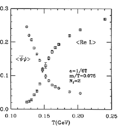
Figure 10: Behavior of the Polyakov loop $<L>$, and the chiral condensate $<\bar{\psi}\psi>$, in 2-Flavor QCD as functions of temperature.

The second is the chiral condensate. While the notion of confinement gets fuzzy in the theory with quarks, the notion of chiral symmetry breaking is perfectly sharp (for massless quarks). And it exhibits very interesting dynamical behavior as a function of temperature. The simplest measure of chiral symmetry breaking is simply the expectation value $\langle\bar{\psi}\psi\rangle$. This quantity is perfectly accessible to lattice gauge theory. In Figure 10, you see that this expectation value does indeed take a dive. In the simulation it does not reach zero, because the quarks are not truly massless, but the possibility of a smooth decrease to zero at a finite value of $T$ is certainly suggested. Studies with varying values of the quark masses, when extrapolated, further support this suggestion.

4 Lecture 3: High-Temperature QCD: Phase Transitions

4.1 Yoga of Phase Transitions and Order Parameters

Confinement, in the pure glue version of QCD (only), is a property we can associate with a definite symmetry, that is valid at low temperature but broken at high temperature. Chiral symmetry, in the versions of QCD with two or more massless quarks is, conversely, spontaneously broken at low temperatures (at least if the number of quarks is not too large) but restored at high temperatures. As emphasized by Landau, the presence or absence of a symmetry is a sharp, objective question, which in any given state of matter must have a yes or no answer. And if the answer is yes in one regime and no in another, passage from one regime to the other must be accompanied by a sharp phase transition. This situation is usually parameterized by some appropriate order parameter, that transforms non-trivially under the symmetry, and is zero on the unbroken side but non-zero on the broken side.

Phase transitions can occur without change of symmetry, or dynamical reasons – we shall see some simple examples below (where there is symmetry lurking just offstage). But by considering changes in symmetry, which must be associated with phase transitions, and behaviors of order parameters we will be able to say quite a lot, without doing any prohibitively difficult calculations.

4.1.1 Second Order Transitions

There are two broad classes of phase transitions, which have quite different qualitative properties near the transition point. First order transition are characterized by a finite discontinuity in the generic thermodynamic parameter – i.e. basically in anything except the free energy, which of course must be equal for the two phases at the transition point. Second-order transitions, on the other hand, are characterized by continuous but nonanalytic behavior of thermodynamic quantities.

In Nature second order transitions are less common than first order transitions, but they are especially interesting. Near first order transitions the two phases are simply ‘different’, and are described by distinct expressions for the free energy (in terms of macroscopic variables). There is a wholesale reorganization of matter, even locally – there are jumps in intensive variables. Near second order transitions that is not the case. In a large but finite volume, a first order transition point will be marked by rare but sudden and drastic jumps from one phase to the other, going over in the infinite volume limit to hysteresis. In the same circumstances, a second order transition point will not exhibit any jumps, and the partition function will be a perfectly analytic function.

So how does the nonanalytic behavior arise? It can only arise from taking the infinite volume limit. This, in turn, implies that for a second order transition to occur there must be low-energy fluctuations of arbitrarily long wave length, since it is only such modes that can render the infinite volume limit subtle (otherwise the free energy must ultimately become simply additive in the volume, for large enough volumes). In terms of static quantities, there must be a diverging correlation length. In terms of particle physics, there must be massless particles. That is, if we quantized the modes under discussion, they would have massless quanta.

The hypothesis – or quasi-theorem, as motivated above – that nonanalytic behavior of thermodynamic quantities near a second order transition must arise from the dynamics of massless modes makes it possible, following Landau and Wilson, to make remarkably concrete and specific predictions about this behavior. The point is that it appears to be very difficult to construct consistent theories of massless particles, unless one considers small numbers of dimensions or large and exotic symmetry structures, that are inappropriate to the cases at hand. So if we specify the desired space dimension and symmetry we may find a unique theory of this kind, or none at all. Then the singular behavior of any possible second-order phase transitions with a given dimensionality and symmetry will be uniquely determined, independent of other details of the underlying microscopic theory. This is the hypothesis of universality.

Universality makes it possible to make rigorous predictions for the behavior of complicated physical systems – such as various versions of QCD – near second-order phase transitions by doing calculations in much simpler models.

Now let me give a few words of orientation about the formal aspects of such analyses, using the three dimensional Ising model as a prototype. We are interested in the singular behavior of thermodynamic functions near a possible second-order phase transition, where the magnetization decreases from a non-zero value to zero. The relevant low-energy, long-wavelength modes are gradual changes in the local average of the magnetization. Since we are working at long wavelengths it is appropriate to coarse grain, so the magnetization is described by a real three-dimensional scalar field $\phi(x)$. We are interested in the singularity of the partition function induced by fluctuations of $\phi(x)$. To find it, we need to construct the appropriate “universal” theory based on $\phi(x)$.

We want this theory to be describing fluctuations that are small in magnitude and long in wavelength, so we should use a Lagrangian with the smallest possible powers of $\phi(x)$ and of derivatives. Of course we need a quadratic term with two derivatives to get any non-trivial spatial behavior at all. To give this term its chance to shine, we will also need to put the mass equal to zero, since a mass term would always dominate the derivative term at long wavelength. Since we have $\phi\rightarrow-\phi$ symmetry, the next possibility is a $\phi^{4}$ term. So our trial ‘Lagrangian’ (to be interpreted as $H/T$, the Hamiltonian divided by the temperature, in statistical mechanical language) is

$$\int d^{3}x{\cal L}~{}=~{}\int d^{3}x(\partial\phi)^{2}+\lambda\phi^{4}~{}.$$ (48)

Now if we count dimensions we see that for the Lagrangian to be dimensionless $\phi$ must have mass dimension $1/2$, and so $\lambda$ must have mass dimension 1. According to naive dimensional analysis, therefore, we are not getting a scale-invariant theory.

We know, however, that interacting field theories contain another source of non-trivial scaling behavior. Because there are an infinite number of degrees of freedom, we must regulate the theory, and define a renormalized coupling at some finite momentum scale, which we fix to a physical value independent of the cutoff. Then in favorable cases we will get cutoff-independent answers, in terms of the renormalized coupling, as we take the cutoff to infinity. We can get a scale invariant theory from this set-up if the bare coupling $\lambda_{b}(\Lambda)$ one needs to insure a fixed renormalized coupling scales as $\lambda_{b}\propto\Lambda^{1\over 2}$. The proportionality constant is then our dimensionless parameter.

That reasoning is quite abstract, so it is informative to consider the situation also from a radically different perspective, due to Wilson and Fisher. We consider, formally, extending the theory to $4-\epsilon$ dimensions. It is of course problematic to construct a field theory in non-integer dimensions, but we can perfectly well continue the perturbation theory integrals, which ought to be adequate if the relevant coupling turns out to be small. Now in $4-\epsilon$ dimensions the same counting as above shows that the mass dimension of $\lambda$ is $\epsilon$. Thus as we rescale the momentum at which the coupling is defined there are two sources of variation. One is simple classical dimensional analysis, which tends to make the $\phi^{4}$ more relevant at small momenta; the other is the running due to fluctuations (loops), familiar in its quantum version from QED or QCD, where it is interpreted as vacuum polarization due to virtual particles. Of course here we are concerned with classical fluctuations, but the equations are just the same. Since $\phi^{4}$ in 4 dimensions is not asymptotically free, the two terms governing renormalization toward the infrared go as

$${d\tilde{\lambda}(p)\over dt}~{}=~{}\tilde{\lambda}\epsilon-b\tilde{\lambda}^{2}~{},$$ (49)

here $t=\ln(p_{0}/p)$, with $p_{0}$ some reference momentum, and $\tilde{\lambda}\equiv\lambda p^{-\epsilon}$, and the equation is valid for $p<<\Lambda$ the cutoff and small $\lambda$ and $\epsilon$. $b$ is a calculable positive number. So as $t\rightarrow\infty$ $\tilde{\lambda}\rightarrow\epsilon/b$, which is indeed small for small enough $\epsilon$. We say there is a fixed-point coupling with this value. With $\Lambda$ fixed, we approach a scale invariant theory for $p<<\Lambda$. The funny dependence of the coupling $\lambda$ (not $\tilde{\lambda}$!) extrapolated to momenta approaching the cutoff – what we would call the bare coupling – on the cutoff $\Lambda$ itself is just what we anticipated before, on abstract grounds.

This construction makes it plausible that there can be a scale-invariant theory, but also makes it clear that this theory will not be easy to find in three dimensions, where the fixed-point coupling cannot be small. One approach, which works remarkably well, is to calculate around $4-\epsilon$ dimensions and extrapolate to $\epsilon=1$. Another is to work directly in three dimensions, calculate to high orders in perturbation theory, and join on to the form at high orders, which is known from sophisticated semiclassical techniques. Finally, one can simply simulate the theory directly numerically. Any of these techniques would be prohibitively difficult to use in high temperature QCD directly, but thanks to universality we can get rigorous quantitative answers (to carefully selected questions, of course!) using much simpler models.

4.1.2 First Order Transitions

An important side-benefit of the analysis of how second-order transitions arise is that it alerts us to cases where this cannot occur. In the Ising model analysis, we found the scale invariant theory could arise when the mass parameter associated with the magnetization vanishes. Since we expect the effective mass parameter to be a function of temperature, $m^{2}=m^{2}(T)$, it is reasonable to expect that this can happen at one particular value of the temperature. So Eqn. 48 is a special case of the embedding set of Lagrangians

$$\int d^{3}x{\cal L}~{}=~{}\int d^{3}x(\partial\phi)^{2}+m^{2}(T)\phi^{2}+\lambda\phi^{4}~{}$$ (50)

describing the dynamics of the fluctuating magnetization not only exactly at, but also near, the critical transition temperature. This is reasonable from another point of view as well: when $m^{2}(T)<0$ a non-zero expectation value for $\phi$ will be preferred, whereas for $m^{2}(T)>0$ the expectation should vanish.

Now if we put the system in an external magnetic field, breaking the $\phi\rightarrow-\phi$ symmetry, then $\phi$ and $\phi^{3}$ terms are allowed. Let’s shift away the $\phi$ term. There will still be a $T$-dependent $m^{2}$, and it can go through zero. But now that will generally not give rise to a second-order transition, because in the presence of a small $\phi^{3}$ term the expectation value will jump to a new minimum at a non-zero (positive) value of $m^{2}$. The special case where the cubic term vanishes simultaneously with $m^{2}$ can be accessed only if there is another control parameter available, in addition to the temperature. Then one has a so-called tricritical point. In the phase plane, the tricritical point appears as the terminus of a line along which there are weaker and weaker first-order transitions.

Even if the mean-field analysis allows a second-order transition, there will not be one if there is no suitable scale-invariant theory to represent the universality class. The mean field analysis ignored fluctuations, but as we have learned these are vital. In our discussion above, we saw that in order to construct the scale-invariant theory we needed to have a simple, finite limiting behavior of the effective coupling under renormalization group transformations toward the infrared. If there is no such limiting behavior, there cannot be a second-order transition. The physical interpretation of this outcome is simply that in such cases the fluctuations have grown out of control, resulting in a catastrophic rearrangement of the state – a first-order transition. Such an eventuality is, for obvious reasons, called a fluctuation driven first-order transition.

Since they are marked by finite discontinuities, first-order transitions are robust against small perturbations. Thus if we have a symmetry and an order parameter, whose change from a non-zero to a zero value forces the existence of a first-order transition according to either of the mechanisms I’ve just discussed, there will still be a first-order transition even if the symmetry is intrinsically slightly broken. There will be no strict order parameter, and thus we would not have been able to predict the necessity of a transition without referring to the nearby, unbroken variant of the theory.

Each and every one of the theoretical phenomena I have mentioned in these orienting sections plays a significant role in understanding the phase structure of QCD!

4.2 Application to Glue Theories

Let’s recall the basic facts. When there are no quarks at all, then there is the possibility of a true confinement-deconfinement transition. As we have discussed, such a transition is characterized by the Polyakov order parameter

$$\langle L\rangle~{}=~{}\langle~{}{\rm Tr}~{}\exp\{i\int_{0}^{\beta}A^{a}_{\tau}\lambda^{a}d\tau\}~{}\rangle.$$ (51)

Here the expectation value is taken over the thermal ensemble of field configurations periodic in imaginary time $\tau$ with period $\beta=1/T$, and $\lambda$ is the representation matrix for the fundamental representation. This loop inserts quark quantum numbers into the ensemble. In the pure glue theory, the operator inserts a flux that cannot be screened, and alters the state by an irreducible amount out to infinity. This costs a finite energy per unit volume, and therefore infinite energy altogether. The expectation value of the loop would therefore be expected to vanish in the confined phase, while it acquires a non-zero value in the unconfined phase. $L$ is multiplied by the appropriate complex root of unity when an element of the center of the gauge group is applied to the state. Thus symmetry under this discrete group (triality for color $SU(3)$, diality for $SU(2)$) is broken in the unconfined phase expected to exist at high temperature.

Since there is a simple order parameter with well-defined symmetry properties, one can entertain the possibility of a second order transition. Indeed there does seem to be a second order transition for $SU(2)$, in the universality class of the (inverted) 3d Ising model. ‘Inverted’ refers to the features that whereas in the Ising model the $Z_{2}$ symmetry is broken at low temperature, but restored at high temperature, the confinement $Z_{2}$ symmetry is valid at low temperature but broken at high temperature. This means the $m^{2}(T)$ goes through zero in the opposite direction, but of course one still has the same universal theory at the critical point and a simple correspondence away from it.

However for $SU(3)$ the appropriate model is different. It is something called the 3-state Potts model. In the field-theoretic version of that model we must use a complex scalar field $\phi$ invariant under $\phi\rightarrow\omega\phi$, with $\omega$ the cube root of unity, to implement the symmetry. With such a field, cubic terms of the type

$$\Delta{\cal L}~{}=~{}\kappa(\phi^{3}+\phi*^{3})$$ (52)

are allowed. The existence of a cubic invariant implies that the transition will be first order.

Both these predictions prove to be true in large-scale numerical simulations of pure glue QCD.

4.3 Application to Chiral Transitions

Again, let’s quickly recall the basics. With dynamical quarks there is no longer a confinement symmetry, but if we have $f$ flavors of massless quarks there is an additional symmetry under chiral transformations in the group $SU(f)_{L}\times SU(f)_{R}\times U(1)_{B}$ of independent special unitary rotations of the left- and right-handed fields, together with the overall vector baryon number symmetry. (The additional apparent axial baryon number symmetry, present at the classical level, is violated in quantum theory by the anomaly, as discussed earlier.) This chiral symmetry is believed on good grounds to break spontaneously down to vector $SU(f)\times U(1)$ at low temperatures; and to be restored at sufficiently high temperatures. Of course for $f=1$ the chiral symmetry is vacuous; but for $f\geq 2$ there is a phase transition associated with restoration of chiral symmetry. Since there is a simple order parameter for this phase transition – namely, for example, the expectation value of the quark bilinear

$$M^{i}_{j}~{}=~{}\langle{\bar{q}_{L}}^{i}{q_{R}}_{j}\rangle$$ (53)

– one may again inquire concerning the possibility of a second order transition.

4.3.1 Formulation of Models

In order to describe a possible second-order transition quantitatively, we must try to find a tractable model in the same universality class. For the chiral order parameter Eqn. 53 the relevant symmetries are independent unitary transformations of the left- and right-handed quark fields, under which

$$M~{}\rightarrow~{}U^{\dagger}MV~{}.$$ (54)

These transformations generate an $SU(f)_{L}\times SU(f)_{R}\times U(1)_{V}$ symmetry, after the anomaly in the axial baryon number current is taken into account. At the phase transition, the true symmetry is broken to $SU(f)_{L+R}\times U(1)_{V}$.

To describe the critical behavior, it is sufficient to retain the degrees of freedom which develop long-range fluctuations at the critical point. It is natural to assume that these are associated with long-wavelength variations in the order parameter, whose magnitude is small and whose variations within the vacuum manifold therefore cost little energy near the transition. Thus the most plausible starting point for analyzing the critical behavior of a possible second-order phase transition in QCD is the Landau-Ginzburg free energy

$${\cal F}={\rm tr}~{}\partial_{i}M^{\dagger}\partial_{i}M~{}+~{}\mu^{2}{\rm tr}~{}M^{\dagger}M~{}+~{}\lambda_{1}{\rm tr}~{}(M^{\dagger}M)^{2}~{}+~{}\lambda_{2}({\rm tr}~{}M^{\dagger}M)^{2}~{}.$$ (55)

Here $\mu^{2}$ is the temperature-dependent renormalized (mass)², which is negative below and positive above the critical point, while $\lambda_{1}$ and $\lambda_{2}$ parameterize the strength of the quartic couplings and are supposed to be smooth at the transition. The symmetry breaking pattern we want is $M\propto{\bf 1}$ below the transition, which is what we shall find at the minimum of the potential, within a range of positive $\lambda_{1}$ and $\lambda_{2}$.

Actually Eqn. 55 is not quite what we want. It has a full $U(f)\times U(f)$ symmetry, which breaks down to $U(f)$. Thus it contains a massless Nambu-Goldstone boson for the axial baryon number symmetry, which is not present in the microscopic theory (QCD) we are trying to model.

For $f=2$ one can solve this problem very neatly by implementing the symmetry in a slightly different way. Instead of general complex matrices, which in this case form a reducible representation of the chiral symmetry, we can restrict ourselves to unitary matrices with positive real determinant. This restriction on $M$ is consistent with the transformation law Eqn. 54 as long as $U$ and $V$ have equal phases, but not if the phases are unequal. Thus the unwanted axial $U(1)$ symmetry is indeed removed. An important point is that for $2\times 2$ matrices the condition of being a multiple of a unitary matrix is a linear condition, so that we can enforce it while remaining within the domain of renormalizable field theories. (Nothing like this is true for larger matrices.) It is very convenient to parameterize the $2\times 2$ matrices in question in terms of four real parameters $(\sigma,\vec{\pi})$ and the Pauli matrices as

$$M~{}=~{}\sigma+i\vec{\pi}\cdot\vec{\tau}~{}.$$ (56)

In this way, we arrive back at the original model of Gell-Mann and Levy.

After this pruning, the order parameter variables that have been retained have the quantum numbers of the scalar isoscalar density $\langle{\bar{q}}^{i}q_{i}\rangle$ and the pseudoscalar isovector densities $\langle{\bar{q}}^{x}\gamma_{5}\vec{\tau}q\rangle$. Furthermore, the two a priori possible quartic couplings $\lambda_{1},\lambda_{2}$ are not independent – a fact which proves to be very significant. In fact the model boils down to the theory of a four-component vector $\phi\equiv(\sigma,\vec{\pi})$ in internal space, that is to say the standard $O(4)$ invariant $n=4$ “Heisenberg magnet”. For smaller numbers of components, this sort of model is a much-studied model for the critical behavior of magnets, with the vector of course representing the magnetization (or staggered magnetization).

For larger values of $f$ the trick discussed above is no longer available. For $f=3,4$ one can break the unwanted $U(1)$ symmetry by adding an additional determinantal interaction ${\rm det}M$. Beyond $f=4$ that too is not entirely satisfactory, because it takes us outside the framework of renormalizable theories in four dimensions (which are suitable starting points for the construction of critical theories, using the $\epsilon$ expansion). However, as will soon appear, in the present context it is almost certainly academic anyway.

4.3.2 Fixed points

Now we may search for second-order transitions within each model, by the standard method of looking for infrared stable fixed points of the renormalization group. The vector model has been studied in great depth, for arbitrary $n$. The existence of a fixed point has been established by detailed analysis of perturbation theory – taken to high orders and supplemented with estimates of the asymptotic behavior directly in three dimensions – directly in three dimensions, and also via the $\epsilon$ expansion. The calculated critical exponents have been successfully compared with appropriate experiments, for $n\leq 3$. Thus there can be no serious doubt that there is a model for a second-order QCD chiral phase transition for two massless quarks, consistent with the symmetry of that theory.

On the other hand for $f\geq 3$ the structure of the renormalization group for the appropriate model is more complicated – there are then two independent couplings, and so to speak more ways to go wrong. In the lowest order of perturbation theory in the $\epsilon$ expansion, the calculations can be done quite simply. They indicate that there is a fixed point of the renormalization group, but that it is not infrared stable. In plain English, this means (if we can trust the $\epsilon$ expansion!) that near the transition one would naively identify by taking $\mu^{2}$ through zero in Eqn. 55 $M$ is actually subject to catastrophic fluctuations, that change the structure of the problem qualitatively. Thus the renormalization group fails to identify a consistent model for a second order transition, and indicates instead that the transition must be a first order transition. In important work Gausterer and Sanielevici have simulated the $f=3$ matrix models directly, both with and without the determinantal interaction, to search for second-order transitions. None was found; the transition is always first order. These authors also studied the $f~{}=~{}2$ model, and did find the expected second-order transition in that case. Thus the expectations drawn from simple $\epsilon$ expansion analysis appear to be vindicated. Direct simulation of the $n=4$ magnet model, and comparison with $f~{}=~{}2$ QCD using the translation dictionary discussed below, is also an attractive possibility.

Existing numerical calculations for QCD, are consistent with the prediction that the proposed models for the universality classes of possible QCD chiral phase transitions are appropriate, and that there is a big difference between the nature of the chiral transition in QCD for $f~{}=~{}2$ and for larger $f$, with the former being second order and the latter first order.

4.4 Close Up on Two Flavors

If we accept that there is a second order transition for $f~{}=~{}2$, we can derive many precise, testable consequences.

As we have just discussed the most plausible starting point for analyzing the critical behavior of a second-order phase transition in QCD is the Landau-Ginzburg free energy

$$F=\int d^{3}x\Bigl{\{}{1\over 2}~{}\partial^{i}\phi^{\alpha}\partial_{i}\phi_{\alpha}~{}+~{}{\mu^{2}\over 2}~{}\phi^{\alpha}\phi_{\alpha}~{}+~{}{\lambda\over 4}(\phi^{\alpha}\phi_{\alpha})^{2}~{}\Bigr{\}}~{},$$ (57)

of an $n=4$ component scalar field. Here $\mu^{2}$ is the temperature-dependent renormalized (mass)², which is negative below and positive above the critical point, while $\lambda$ is the strength of the quartic couplings and is supposed to be smooth at the transition. We neglect terms with higher powers of $\phi$ since $|\phi|$ is small near the transition. The symmetry breaking pattern we want is ${\cal M}\propto{\bf 1}$ (equivalently, $\langle\sigma\rangle\neq 0;\langle\vec{\pi}\rangle=0$) below the transition which is indeed what we find at the minimum of the potential for positive $\lambda$. This model has been studied in depth for arbitrary $\eta$ and spatial dimension $d$, and the existence of an infrared stable fixed point of the renormalization group for $\eta=4$, $d=3$ is firmly established. Hence, it is a model for a second order QCD chiral phase transition for two massless quarks.

When the free energy Eqn. 57 is written in terms of $\sigma$ and $\vec{\pi}$ it looks much like the original model of Gell-Mann and Levy. But there are two changes: there are no nucleon fields and only three (spatial) dimensions. These two changes reflect an important distinction. We are only proposing Eqn. 57 as appropriate near the second order phase transition point. This is because it is only there that we can appeal to universality – the long-wavelength behavior of the $\sigma$ and $\vec{\pi}$ fields is determined by the infrared fixed point of the renormalization group, and microscopic considerations are irrelevant to it. In Euclidian field theory at finite temperature, the integral over $\omega$ of zero temperature field theory is replaced by a sum over Matsubara frequencies $\omega_{n}$ given by $2n\pi T$ for bosons and $(2n+1)\pi T$ for fermions with $n$ an integer. Hence, one is left with a Euclidian theory in three spatial dimensions with massless fields from the $n=0$ terms in the boson sums and massive fields from the rest of the boson sums and the fermion sums. Hence, to discuss the massless modes of interest at the critical point, Eqn. 57 is sufficient. We do not need to introduce nucleon fields or constituent quark fields.

4.4.1 Critical Exponents

The most important universal properties of the second order transition are the critical exponents, which we now define.

First, let us introduce the reduced temperature $t~{}=~{}(T-T_{c})/T_{c}$. The exponents $\alpha$, $\beta$, $\gamma$, $\eta$, and $\nu$ describe the singular behavior of the theory with strictly zero quark masses as $t\rightarrow 0$. For the specific heat one finds

$$C(T)\sim|t|^{-\alpha}+{\rm less~{}singular.}$$ (58)

The behavior of the order parameter defines $\beta$.

$$\langle|\phi|\rangle\sim|t|^{\beta}~{}~{}{\rm for}~{}t<0~{}.$$ (59)

$\eta$ and $\nu$ describe the behavior of the correlation length $\xi$ where

$$G_{\alpha\beta}(x)~{}\equiv~{}\langle\phi(x)_{\alpha}\phi(0)_{\beta}\rangle-\langle\phi_{\alpha}\rangle\langle\phi_{\beta}\rangle~{}\rightarrow~{}\delta_{\alpha\beta}{A\over|x|}\exp(-|x|/\xi)~{}~{}{\rm at~{}large~{}distances.}$$ (60)

$A$ is independent of $|x|$, but may depend on $t$. The correlation length exponent $\nu$ is defined by

$$\xi\sim|t|^{-\nu}~{}.$$ (61)

Above $T_{c}$, where the correlation lengths are equal in the sigma and pion channels, the susceptibility exponent $\gamma$ is defined by

$$\int d^{3}x~{}G_{\alpha\beta}(x)\sim t^{-\gamma}.$$ (62)

The exponent $\eta$ is defined through the behavior of the Fourier transform of the correlation function:

$$G_{\alpha\beta}(k\rightarrow 0)\sim k^{-2+\eta}~{}.$$ (63)

The last exponent, $\delta$ is related to the behavior of the system in a small magnetic field $H$ which explicitly breaks the $O(4)$ symmetry. Let us first show that in a QCD context, $H$ is proportional to a common quark mass $m_{u}=m_{d}\equiv m_{q}$. This common mass term may be represented by a $2\times 2$ matrix ${\cal D}$ given by $m_{q}$ times the identity matrix. We are now allowed to construct the free energy from invariants involving both ${\cal D}$ and ${\cal M}$. The lowest dimension term linear in ${\cal D}$ is just ${\rm tr}{\cal M}^{\dagger}{\cal D}=m_{q}\sigma$, which in magnet language is simply the coupling of the magnetization to an external field $H\propto m_{q}$. In the presence of an external field, the order parameter is not zero at $T_{c}$. In fact,

$$\langle|\phi|\rangle(t=0,H\rightarrow 0)\sim H^{1/\delta}~{}.$$ (64)

The six critical exponents defined above are related by four scaling relations. These are

$$\alpha~{} =~{}2-d\nu$$

$$\beta~{} =~{}{\nu\over 2}(d-2+\eta)$$

$$\gamma~{} =~{}(2-\eta)\nu$$

$$\delta~{} =~{}{d+2-\eta\over d-2+\eta}~{}.$$ (65)

We therefore need values for $\eta$ and $\nu$ for the four component magnet in $d=3$. These were obtained in the remarkable work of Baker, Meiron and Nickel, who carried the perturbation theory to seven-loop order, and used information about the behavior of asymptotically large orders, and conformal mapping and Padé approximant techniques to obtain

$$\eta~{} =~{}~{}.03\pm.01$$

$$\nu~{} =~{}~{}.73\pm.02~{}.$$ (66)

Using Eqn. 4.4.1, the remaining exponents are $\alpha=-0.19\pm.06$, $\beta=0.38\pm.01$, $\gamma=1.44\pm.04$ and $\delta=4.82\pm.05$. Since $\alpha$ is negative there is a cusp in the specific heat at $T_{c}$, rather than a divergence.

A more powerful result which includes Eqn. 59 and Eqn. 64 as special cases is the critical equation of state:

$$H~{}=~{}M|M|^{\delta-1}\kappa_{1}g(\kappa_{2}t|M|^{-{1\over\beta}})$$ (67)

in which here $H~{}\equiv~{}m$, $M~{}\equiv~{}\langle{\bar{q}}q\rangle=\langle|\phi|\rangle$, $t~{}\equiv~{}(T-T_{c})/T_{c}$, $g$ is a universal function, and $\kappa_{1}$ and $\kappa_{2}$ are non-universal constants. This equation of state could, of course, be compared directly with sufficiently accurate numerical simulations.

4.4.2 Tricritical Point

To this point I have been discussing a world with two massless quarks, and so we have implicitly been taking the strange quark mass to be infinite. On the other hand, I argued earlier that if the strange quark is massless, then the chiral phase transition is first order. Hence, as the strange quark mass is reduced from infinity to zero, at some point the phase transition must change from second order to first order. This point is called a tricritical point. There is numerical evidence that when the strange quark has its physical mass, and the two light quarks are taken strictly massless, the transition is second order, with the consequences discussed above. However this conclusion was controversial for many years, and even now may not be completely secure. In any case the physical strange quark mass is not drastically different from the critical value, so let’s indulge our idle curiosity a little further (this will pay off shortly).

In a lattice simulation, the strange quark mass can be tuned to just the right value to reach the tricritical point. Let’s discuss the critical exponents that would be observed in such a simulation.

Let us consider the effect of adding a massive but not infinitely massive strange quark to the two flavor theory. This will not introduce any new fields which become massless at $T_{c}$, and so the arguments leading to the free energy Eqn. 57 are still valid. The only effect of the strange quark, then, is to renormalize the couplings. Renormalizing $\mu^{2}$ simply shifts $T_{c}$, as does renormalizing $\lambda$ unless $\lambda$ becomes negative. In that case, one can no longer truncate the Landau-Ginzburg free energy at fourth order. After adding a sixth order term, and keeping track of small light quark masses, the free energy becomes

$$F=\int d^{3}x\Bigl{\{}{1\over 2}(\nabla\phi)^{2}+{\mu^{2}\over 2}\phi^{2}+{\lambda\over 4}(\phi^{2})^{2}+{\kappa\over 6}(\phi^{2})^{3}-H\sigma\Bigr{\}}~{}.$$ (68)

While for positive $\lambda$, $\phi^{2}$ increases continuously from zero as $\mu^{2}$ goes through zero, for negative $\lambda$, $\phi^{2}$ jumps discontinuously from zero to $|\lambda|/(2\kappa)$ when $\mu^{2}$ goes through $\lambda^{2}/(4\kappa)$. Hence, the phase transition has become first order. Thus at the value of $m_{s}$ where $\lambda=0$, the phase transition changes continuously from second order to first order.

The singularities of thermodynamic functions near tricritical points, like the singularities near ordinary critical points, are universal. Hence, it is natural to propose that QCD with two massless flavors of quarks and with $T$ near $T_{c}$ and $m_{s}$ near its tricritical value is in the universality class of the $\phi^{6}$ Landau-Ginzburg model Eqn. 68 . This model has been studied extensively. Because the $\phi^{6}$ interaction is strictly renormalizable in three dimensions, this model is much simpler to analyze than the $\phi^{4}$ model of the ordinary critical point. No $\epsilon$ expansion is necessary, and the critical exponents all take their mean field values, up to calculable logarithmic corrections. Here I’ll be content to show you the mean field tricritical exponents.

In mean field theory, the correlation function in momentum space is simply $G_{\alpha\beta}(k)=\delta_{\alpha\beta}(k^{2}+\mu^{2})^{-1}$. Since $\mu^{2}\sim t$, this gives the exponents $\eta=0$, $\gamma=1$ and $\nu=1/2$. To calculate $\alpha$ and $\beta$, we minimize $F$ for $H=\lambda=\nabla\phi=0$, and find $\alpha=1/2$ and $\beta=1/4$. To calculate $\delta$, we minimize $F$ for $t=\lambda=\nabla\phi=0$ and find $\delta=5$.

The result for the specific heat exponent $\alpha$ is particularly interesting, since it means that the specific heat diverges at the tricritical point, unlike at the ordinary critical point. This means that whereas for $m_{s}$ large enough that the transition is second order the specific heat $C(T)$ has a cusp but is finite at $T=T_{c}$, as $m_{s}$ is lowered to the tricritical value $C(T_{c})$ should increase since at the tricritical point it diverges. This behavior should be seen in future lattice simulations.

Finally, at a tricritical point there is one more relevant operator than at a critical point, since two physical quantities ($t$ and $m_{s}$) must be tuned to reach a tricritical point. Hence, a new exponent $\phi_{t}$, the crossover exponent, is required. For $\lambda\neq 0$, tricritical behavior will be seen only for $|t|>t^{*}$, while for $|t|<t^{*}$, either ordinary critical behavior or first order behavior (depending on the sign of $\lambda$) results. $t^{*}$ depends on $\lambda$ according to

$$t^{*}\sim\lambda^{1/\phi_{t}}$$ (69)

The mean field value of $\phi_{t}$ is obtained by minimizing the free energy $F$ for $H=\nabla\phi=0$, and is $\phi_{t}=1/2$. These mean field tricritical exponents, $\alpha=1/2$, $\beta=1/4$, $\gamma=1$, $\delta=5$, $\eta=0$, $\nu=1/2$, and $\phi_{t}=1/2$ would describe the real world if $m_{s}$ were smaller than it is, and will describe future lattice simulations with $m_{s}$ chosen appropriately.

4.4.3 Robustness

If we now turn on small but non-zero $u$ and $d$ quark masses, the first-order line will persist, but the second-order transition will disappear, replaced by a crossover. And there will still be a true (tri)critical point, where the first-order line terminates! It will be in the universality class of a liquid-gas or Ising tricritical point, rather than the asymptotically free $\phi^{6}$-type theory.

4.5 A Genuine Critical Point! (?)

In reality, of course, we cannot vary the strange quark mass. If the strange quark mass is, as seems to be indicated, so large that for massless $u$ and $d$ quarks we would have a second-order transition, then after taking into account the non-zero mass of these quarks we are left with only a crossover. Moreover since the mass of the physical pions is not so different from the critical temperature, we cannot expect that correlation length ever gets very long. Thus we are left with a crossover, and perhaps not a very dramatic one. This is a definite prediction, though perhaps a disappointing one for experimentalists, of the form “nothing striking occurs” (in the way of sharp phase transitions). But fortunately, as emphasized in recent work of Stephanov, Rajagaopal, and Shuryak, that is not the end of the story.

Their basic insight is that although one cannot vary the strange quark mass experimentally, there is another control parameter that one can vary – the chemical potential. If the singularity in $T$ at slightly unphysical values of $m_{s}$ and zero $\mu$ continues into a singularity at the physical value of $m_{s}$ for slightly costive $\mu$, we will be back in business, with a true physical (tri)critical point, featuring diverging correlation lengths at a particular point in the $\mu,T$ plane.

4.5.1 Subnuclear Boiling

The same structure is also suggested by an entirely different line of thought. Consider now the behavior of two-flavor QCD as one varies the chemical potential $\mu$ at zero temperature. Models of the type we will be considering in the next two lectures suggest that in the case of two mass quarks there is a first-order transition from a state of broken chiral symmetry at $\mu=0$ to a state with chiral symmetry restored at large $\mu$. Since the transition is first order, it remains as a first-order transition in the presence of small symmetry-breaking perturbations (the quark masses), despite the absence of an order parameter. This idea is very much in the spirit of the phenomenologically successful MIT bag model, in which nucleons are pictured as droplets of chiral symmetry restored phase embedded in a broken symmetry vacuum. Indeed, if true, it comes very close to providing a microscopic justification of that model.

Physically, the suggested transition represents a sort of subnuclear boiling, to a phase in which quarks (or at least, as we shall see, a subset of them) are liberated to behave as nearly massless, weakly interacting particles.

If in fact there is such a transition, it becomes interesting to follow its fate as a function of temperature. At small temperatures, we shall still have a first-order transition at some value $\mu_{c}(T)$. We might expect that $\mu_{c}(T)$ decreases with $T$, since higher temperature should favor the higher-entropy ‘boiled’ state. This expectation can be convincingly justified on thermodynamic grounds. But we know that $\mu_{c}(T)$ cannot decrease to zero, since for $\mu=0$ we have only a crossover. Again, the simplest possibility to reconcile the behaviors along the axes is to suppose that the line of first-order transitions terminates at a definite $(\mu_{t},T_{t})$. The strength of the first-order transition weakens as a function of temperature, until at $T_{t}$ the strict distinction between hadron and quark phases has disappeared. This $(\mu_{t},T_{t})$ is the ripe fruit of our theoretical labors: the prediction of a true (tri)critical point in honest-to-god real world QCD, arrived at from qualitative, but deeply rooted, theoretical considerations!

4.5.2 Physical Signatures

Stephanov, Rajagopal and Shuryak (SRS) have made quite specific and detailed proposals for experimental signatures of the phase transition. A proper discussion of this would take us far afield, but a few comments are in order.

In a heavy ion collision one produces a baryon number poor fireball in the central region, but toward the fragmentation regions the baryon number density increases. As the different parts of the fireball expand and cool, each part traces out a different history in the $(\mu,T)$ plane. There will be critical fluctuations and long correlation lengths in a given region of phase space if – and only if – material in the region has passed close close to $P=(\mu_{t},T_{t})$ during its history. For that class of events and regions of rapidity space, one can expect enhanced multiplicities of, and correlations among, low-momentum pions. These enhancements will have the distinctive feature of being non-monotonic in the experimental control parameters, since one can miss the critical point on either of two sides.

The simplest observables to analyze are the event-by-event fluctuations of the mean transverse momentum of the charged particles in an event, $p_{T}$, and of the total charged multiplicity in an event, $N$. SRS calculate the magnitude of the effects of critical fluctuations on these and other observables, making predictions which, they hope, will allow experiments to find. As a necessary prelude, they analyze the contribution of noncritical thermodynamic fluctuations. They find that NA49 data (hep-ex/9904014) is consistent with the hypothesis that most of the event-by-event fluctuation observed in the data is thermodynamic in origin. This bodes well for the detectability of systematic changes in thermodynamic fluctuations near $P$.

As one example, consider the ratio of the width of the true event-by-event distributions of $p_{T}$ to the width of the distribution in a sample of mixed events. SRS call this ratio $\sqrt{F}$. NA49 has measured $\sqrt{F}=1.002\pm 0.0002$, which is consistent with expectations for noncritical thermodynamic fluctuations. A detailed calculation suggests that critical fluctuations can increase $\sqrt{F}$ by 10 - 20%, fifty times the statistical error in the present measurement. There are other observables which are even more sensitive to critical effects. For example, a $\sqrt{F_{\rm soft}}$ defined by using only the 10% softest pions in each event, might well be affected at the factor of two level.

NA49 data demonstrates very clearly that SPS collisions at $\sqrt{s}$ = 17 GeV do not freeze out near the critical point. $P$ has not yet been discovered. The nonmonotonic appearance and then disappearance (as $\sqrt{s}$ is varied) of any one of the signatures of the critical fluctuations mentioned above, or others, would be strong evidence for critical fluctuations. If nonmonotonic variation is seen in several of these observables, with the maxima in all signatures occurring at the same value of $\sqrt{s}$, it would turn strong evidence into an unambiguous discovery of the critical point. The quality of the present NA49 data, and the confidence with which we can use it to learn that collisions at $\sqrt{s}$ = 17 GeV 17 GeV do not freeze out near the critical point make it plausible that critical behavior, if present, could be discerned experimentally. If and when the critical point $P$ is discovered, it will appear prominently on the map of the phase diagram featured in any future textbook of QCD.

4.5.3 Wanted: Numerical Data

The web of general arguments I have outlined above seems to me to make it quite plausible that there is a true critical point in QCD. We can invoke the canonical yoga of second-order phase transitions to make precise, quantitive predictions for the singular behavior of thermodynamics near this point. Arguments of this sort, however, cannot address the non-universal but vital question of precisely where $(\mu_{t},T_{t})$ is. It is a great challenge to locate this point theoretically, and of course such knowledge, even if approximate, would greatly simplify the experimentalist search.

I believe it ought to be possible to locate the tricritical point numerically. For while it is notoriously difficult to deal with large chemical potentials at small temperature numerically, there are good reasons to be optimistic about high temperatures and relatively small chemical potentials, which is our concern here. Some combination of extrapolating from data taken at imaginary values of the chemical potential, and/or using the real part of the fermion determinant as the measure, may be adequate to sense the singularity, especially if we dial the strange quark mass to bring it close to $\mu=0$ (and then extrapolate back to the physical strange quark mass).

If all these strands can be brought together, it will be a wonderful interweaving of theory, experiment, and numerics.

5 Lecture 4: High-Density QCD: Methods

The behavior of QCD at high density is intrinsically interesting, as the answer to the question: What happens to matter, if you keep squeezing it harder and harder? It is also directly relevant to the description of neutron star interiors, neutron star collisions, and events near the core of collapsing stars. Also, one might hope to obtain some insight into physics at “low” density – that is, ordinary nuclear density or just above – by approaching it from the high-density side.

5.1 Hopes, Doubts, and Fruition

Why might we anticipate QCD simplifies in the limit of high density? A crude answer is: “Asymptotic freedom meets the Fermi surface.” One might argue, formally, that the only external mass scale characterizing the problem is the large chemical potential $\mu$, so that if the effective coupling $\alpha_{s}(\mu)$ is small, as it will be for $\mu\gg\Lambda_{QCD}$, where $\Lambda_{QCD}\approx 200$ Mev is the primary QCD scale, then we have a weak coupling problem. More physically, one might argue that at large $\mu$ the relevant, low-energy degrees of freedom involve modes near the Fermi surface, which have large energy and momentum. An interaction between particles in these modes will either barely deflect them, or will involve a large momentum transfer. In the first case we don’t care, while the second is governed by a small effective coupling.

These arguments are too quick, however. The formal argument is specious, if the perturbative expansion contains infrared divergences. And there are good reasons – two separate ones, in fact – to anticipate such divergences.

First, Fermi balls are generically unstable against the effect of attractive interactions, however weak, between pairs near the Fermi surface that carry equal and opposite momentum. This is the Cooper instability, which drives ordinary superconductivity in metals and the superfluidity of He3. It is possible to have an instability at arbitrarily weak coupling because occupied pair states can have very low energy, and they can all scatter into one another. Thus one is doing highly degenerate perturbation theory, and in such a situation even a very weak coupling can produce significant “nonperturbative” effects.

Second, nothing in our heuristic argument touches the gluons. To be sure the gluons will be subject to electric screening, but at zero frequency there is no magnetic screening, and infrared divergences do in fact arise, through exchange of soft magnetic gluons.

Fortunately, by persisting along this line of thought we find a path through the apparent difficulties. Several decades ago Bardeen, Cooper, and Schrieffer taught us, in the context of metallic superconductors, how the Cooper instability is resolved. We can easily adapt their methods to QCD. In electronic systems only rather subtle mechanisms can generate an attractive effective interaction near the Fermi surface, since the primary electron-electron interaction is Coulomb repulsion. In QCD, remarkably, it is much more straightforward. Even at the crudest level we find attraction. Indeed, two quarks, each a color triplet, can combine to form a single color antitriplet, thus reducing their total field energy.

The true ground state of the quarks is quite different from the naive Fermi balls. It is characterized by the formation of a coherent condensate, and the development of an energy gap. The condensation, which is energetically favorable, is inconsistent with a magnetic color field, and so such weak magnetic color fields are expelled. This is the color version of the famous Meissner effect in superconductivity, which is essentially identical to what is known as the Higgs phenomenon in particle physics. Magnetic screening of gluons, together with energy gaps for quark excitations, remove the potential sources of infrared divergences mentioned above. Thus we have good reasons to hope that a weak coupling – though, of course, nonperturbative – treatment of the high density state will be fully consistent and accurate.

The central result in recent developments is that this program can be carried to completion rigorously in QCD with sufficiently many (three or more) quark species. Thus the more refined, and fully adequate, answer to our earlier question is: “Asymptotic freedom meets the BCS groundstate.” Together, these concepts can render the behavior of QCD at asymptotically high density calculable.

5.2 Another Renormalization Group

To sculpt the problem, begin by assuming weak coupling, and focus on the quarks. Then the starting point is Fermi balls for all the quarks, and the low-energy excitations include states where some modes below the nominal Fermi surface are vacant and some modes above are occupied. The renormalization group, in a generalized sense, is a philosophy for dealing with problems involving nearly degenerate perturbation theory. In this approach, one attempts to map the original problem onto a problem with fewer degrees of freedom, by integrating out the effect of the higher-energy (or, in a relativistic theory, more virtual) modes. Then one finds a new formulation of the problem, in a smaller space, with new couplings. In favorable cases the reformulated problem is simpler than the original, and one can go ahead and solve it.

This account of the renormalization group might seem odd, at first sight, to high-energy physicists accustomed to using asymptotic freedom in QCD. That is because in traditional perturbative QCD one runs the procedure backward. When one integrates out highly virtual modes, one finds the theory becomes more strongly coupled. Simplicity arises when one asks questions that are somehow inclusive, so that to answer them one need not integrate out very much. It is then that the microscopic theory, which is ideally symmetric and constrained, applies directly. So one might say that the usual application of the renormalization group in QCD is fundamentally negative: it informs us how the fundamentally simple theory comes to look complicated at low energy, and helps us to identify situations where we can avoid the complexity.

Figure 11: Graph contributing to the renormalization of four-fermion couplings.

Here, although we are still dealing with QCD, we are invoking quite a different renormalization group, one which conforms more closely to the Wilsonian paradigm. We consider the effect of integrating out modes whose energy is within the band $(\epsilon,\delta\epsilon)$ of the Fermi surface, on the modes of lower energy. This will renormalize the couplings of the remaining modes, due to graphs like those displayed in Figure 11. In addition the effect of higher-point interactions is suppressed, because the phase space for them shrinks, and it turns out that only four-fermion couplings survive unscathed (they are the marginal, as opposed to irrelevant, interactions). Indeed the most significant interactions are those involving particles or holes with equal and opposite three momenta, since they can scatter through many intermediate states. For couplings $g_{\eta}$ of this kind we find

$${dg_{\eta}\over d\ln\delta}=\kappa_{\eta}g_{\eta}^{2}.$$ (70)

Here $\eta$ labels the color, flavor, angular momentum, … channel and in general we have a matrix equation – but let’s keep it simple, so $\kappa_{\eta}$ is a positive number. Then Eqn. 70 is quite simple to integrate, and we have

$${1\over g_{\eta}(1)}-{1\over g_{\eta}(\delta)}=\kappa_{\eta}\ln\delta.$$ (71)

Thus for $g_{\eta}(1)$ negative, corresponding to attraction, $|g_{\eta}(\delta)|$ will grow as $\delta\rightarrow 0$, and become singular when

$$\delta=e^{1\over\kappa_{\eta}g_{\eta}(1)}.$$ (72)

Note that although the singularity occurs for arbitrarily weak attractive coupling, it is nonperturbative.

5.3 Pairing Theory

The renormalization group toward the Fermi surface helps us identify potential instabilities, but it does not indicate how they are resolved. The great achievement of BCS was to identify the form of the stable ground state the Cooper instability leads to. Their original calculation was variational, and that is still the most profound and informative approach, but simpler, operationally equivalent algorithms are now more commonly used. I will be very sketchy here, since this is textbook material.

The simplest and most beautiful results, luckily, occur in the version of QCD containing three quarks having equal masses. I say luckily, because this idealization applies to the real world, at densities so high that we can neglect the strange quark mass (yet not so high that we have to worry about charmed quarks). Until further notice, I’ll be focusing on this case.

Most calculations to date have been based on model interaction Hamiltonians, that are motivated, but not strictly derived, from microscopic QCD. They are chosen as a compromise between realism and tractability. For concreteness I shall here follow, and consider

$$\begin{array}[]{ll}H&=\displaystyle\int d^{3}x\,{\bar{\psi}}(x)(\nabla\!\!\!\!/\,-\mu\gamma_{0})\psi(x)+H_{I},\\ H_{I}&=K\displaystyle\sum_{\mu,A}\int d^{3}x\,{{\cal F}}{\bar{\psi}}(x)\gamma_{\mu}T^{A}\psi(x)\ {\bar{\psi}}(x)\gamma^{\mu}T^{A}\psi(x)\end{array}$$ (73)

Here the $T^{A}$ are the color $SU(3)$ generators, so the quantum numbers are those of one-gluon exchange. However instead of an honest gluon propagator we use an instantaneous contact interaction, modified by a form-factor $\cal F$. $\cal F$ is taken to be a product of several momentum dependent factors $F(p)$, one for each leg, and to die off at large momentum. One convenient possibility is $F(p)=(\lambda^{2}/(p^{2}+\lambda^{2}))^{\nu}$, where $\lambda$ and $\nu$ can be varied to study sensitivity to the location and shape of the cutoff. The qualitative effect of the form-factor is to damp the spurious ultraviolet singularities introduced by $H_{I}$; microscopic QCD, of course, does have good ultraviolet behavior. One will tend to trust conclusions that do not depend sensitively on $\lambda$ or $\nu$. In practice, one finds that the crucial results – the form and magnitude of gaps – are rather forgiving.

Given the Hamiltonian, we can study the possibilities for symmetry breaking condensations. The most favorable condensation possibility so far identified is of the form

$$\begin{array}[]{lll}~{}\langle q^{i\alpha}_{La}(p)q^{j\beta}_{Lb}(-p)\rangle~{}=~{}-\langle q^{i\alpha}_{Ra}(p)q^{j\beta}_{Rb}(-p)\rangle~{}=~{}\epsilon^{ij}(\kappa_{1}(p^{2})\delta^{\alpha}_{a}\delta^{\beta}_{b}+\kappa_{2}(p^{2})\delta^{\alpha}_{b}\delta^{\beta}_{a})~{}.\end{array}$$ (74)

Here we encounter the phenomenon of color-flavor locking. The ground state contains correlations whereby both color and flavor symmetry are spontaneously broken, but the diagonal subgroup, which applies both transformations simultaneously, remains valid. There are several good reasons to think that condensation of this form characterizes the true ground state, with lowest energy, at asymptotic densities. It corresponds to the most singular channel, in the renormalization group analysis discussed above. It produces a gap in all channels, and is perturbatively stable, so that it is certainly a convincing local minimum. It resembles the known order parameter for the B phase of superfluid He3. And it beats various more-or-less plausible competitors that have been investigated, by a wide margin.

Given the form of the condensate, one can fix the leading functional dependencies of $\kappa_{1}(p^{2},\mu)$ and $\kappa_{2}(p^{2},\mu)$ at weak coupling by a variational calculation. For present purposes, it is adequate to replace all possible contractions of the quark fields in Eqn. 73 having the quantum numbers of Eqn. 74 with their supposed expectation values, and diagonalize the quadratic part of the resulting Hamiltonian. The ground state is obtained, of course, by filling the lowest energy modes, up to the desired density. One then demands internal consistency, i.e. that the postulated expectation values are equal to the derived ones. Some tricky but basically straightforward algebra leads us to the result

$$\Delta_{1,8}(p^{2})=F(p)^{2}\Delta_{1,8}$$ (75)

where $\Delta_{1}$ and $\Delta_{8}$ satisfy the coupled gap equations

$$\begin{array}[]{ll}\Delta_{8}+{1\over 4}\Delta_{1}&={16\over 3}KG(\Delta_{1})\\ \vskip 6.0pt plus 2.0pt minus 2.0pt\cr{1\over 8}\Delta_{1}&={16\over 3}KG(\Delta_{8})\end{array}$$ (76)

where we have defined

$$G(\Delta)=-{1\over 2}\sum_{{\bf k}}\Biggl{\{}{F(k)^{4}\Delta\over\sqrt{(k-\mu)^{2}+F(k)^{4}\Delta^{2}}}+{F(k)^{4}\Delta\over\sqrt{(k+\mu)^{2}+F(k)^{4}\Delta^{2}}}\Biggr{\}}$$ (77)

and

$$\begin{array}[]{ll}\kappa_{1}(p^{2})&={1\over 8K}(\Delta_{8}(p^{2})+{1\over 8}\Delta_{1}(p^{2}))\\ \vskip 6.0pt plus 2.0pt minus 2.0pt\cr\kappa_{2}(p^{2})&={3\over 64K}\Delta_{1}(p^{2}).\end{array}$$ (78)

The $\Delta$ are defined so that $F(p)^{2}\Delta_{1,8}(p^{2})$ are the gaps for singlet or octet excitations at 3-momentum $p$. Eqn. 76 must be solved numerically.

Finally, to obtain quantitative estimates of the gaps, we must normalize the parameters of our model Hamiltonian. One can do this very crudely by using the model Hamiltonian in the manner originally pioneered by Nambu and Jona-Lasinio, that is as the basis for a variational calculation of chiral symmetry breaking at zero density. The magnitude of this chiral condensate can then be fixed to experimental or numerical results. In this application we have no firm connection between the model and microscopic QCD, because there is no large momentum scale (or weak coupling parameter) in sight. Nevertheless a very large literature following this approach encourages us to hope that its results are not wildly wrong, quantitatively. Upon adopting this normalization procedure, one finds that gaps of order several tens of Mev near the Fermi surface are possible at moderate densities.

While this model treatment captures major features of the physics of color-flavor locking, with a little more work it is possible to do a much more rigorous calculation, and in particular to normalize directly to the known running of the coupling at large momentum. I’ll now sketch .

5.4 Taming the Magnetic Singularity

A proper discussion of the fully microscopic calculation is necessarily quite technical, and would be out of place here, but the spirit of the thing – and one of the most striking results – can be conveyed simply.

When retardation or relativistic effects are important a Hamiltonian treatment is no longer appropriate. One must pass to Lagrangian and graphical methods. (Theoretical challenge: is it possible to systematize these in a variational approach?) The gap equation appears as a self-consistency equation for the assumed condensation, shown graphically in Figure 12.

Figure 12: Graphical form of the self-consistent equation for the condensate (gap equation).

With a contact interaction, and throwing away manifestly spurious ultraviolet divergences, we obtain a gap equation of the type

$$\Delta\propto g^{2}\int d\epsilon{\Delta\over\sqrt{\epsilon^{2}+\Delta^{2}}}.$$ (79)

The phase space transverse to the Fermi surface cancels against a propagator, leaving the integral over the longitudinal distance $\epsilon$ to the Fermi surface. Note that the integral on the right diverges at small $\epsilon$, so that as long as the proportionality constant is positive one will have non-trivial solutions for $\Delta$, no matter how small is $g$. Indeed, one finds that for small $g$, $\Delta\sim e^{-{\rm const}/g^{2}}$.

If we restore the gluon propagator, we will find a non-trivial angular integral, which diverges for forward scattering. That divergence will be killed, however, if the gluon acquires a mass $\propto g\Delta$ through the Meissner-Higgs mechanism. Thus we arrive at a gap equation of the type

$$\Delta\propto g^{2}\int d\epsilon{\Delta\over\sqrt{\epsilon^{2}+\Delta^{2}}}dz{\mu^{2}\over\mu^{2}+(g\Delta)^{2}}.$$ (80)

Now one finds $\Delta\sim e^{-{\rm const}/g}$!

A proper discussion of the microscopic gap equation is considerably more involved than this, but the conclusion that the gap goes exponentially in the inverse coupling (rather than its square) at weak coupling still emerges. It has the amusing consequence, that at asymptotically high densities the gap becomes arbitrarily large! This is because asymptotic freedom insures that it is the microscopic coupling $1/g(\mu)^{2}$ which vanishes logarithmically, so that $e^{-{\rm const}/g(\mu)}$ does not shrink as fast as $1/\mu$. Since the “dimensional analysis” scale of the gap is set by $\mu$, its linear growth wins out asymptotically.

6 Lecture 5: High-Density QCD: Color-Flavor Locking and Quark-Hadron Continuity

Color-flavor locking has many remarkable consequences. There is a gap for all colored excitations, including the gluons. This is, operationally, confinement. The photon picks up a gluonic component of just such a form as to ensure that all elementary excitations, including quarks, are integrally charged. Some of the gluons acquire non-zero, but integer-valued, electric charges. Baryon number is spontaneously broken, which renders the high-density material a superfluid.

If in addition the quarks are massless, then their chiral symmetry is spontaneously broken, by a new mechanism. The left-dynamics and the right-dynamics separately lock to color; but since color allows only vector transformations, left is thereby locked to right.

You may notice several points of resemblance between the low-energy properties calculated for the high-density color-flavor locked phase and the ones you might expect at low density, based on semi-phenomenological considerations such as the MIT bag model, or experimental results in real-world QCD. The quarks play the role of low-lying baryons, the gluons play the role of the low-lying vector mesons, and the Nambu-Goldstone bosons of broken chiral symmetry play the role of the pseudoscalar octet. All the quantum numbers match, and the spectrum has gaps – or not – in all the right places. In addition we have baryon number superfluidity, which extends the expected pairing phenomena in nuclei. Overall, there is an uncanny match between all the universal, and several of the non-universal, features of the calculable high-density and the expected low-density phase. This leads us to suspect that there is no phase transition between them!

6.1 Gauge Symmetry (non)-Breaking

An aspect of Eqn. 74 that might appear troubling at first sight, is its lack of gauge invariance. There are powerful general arguments that local gauge invariance cannot be broken. Indeed, local gauge invariance is really a tautology, stating the equality between redundant variables. Yet its ‘breaking’ is central to two of the most successful theories in physics, to wit BCS superconductivity theory and the standard model of electroweak interactions. In BCS theory we postulate a non-zero vacuum expectation value for the (electrically charged) Cooper pair field, and in the standard model we postulate a non-zero vacuum expectation value for the Higgs field, which violates both the weak isospin SU(2) and the weak hypercharge U(1).

In each case, we should interpret the condensate as follows. We are working in a gauge theory at weak coupling. It is then very convenient to fix a gauge, because after we have done so – but not before! – the gauge potentials will make only small fluctuations around zero, which we will be able to take into account perturbatively. Of course at the end of any calculation we must restore the gauge symmetry, by averaging over the gauge fixing parameters (gauge unfixing). Only gauge-invariant results will survive this averaging. In a fixed gauge, however, one might capture important correlations, that characterize the ground state, by specifying the existence of non-zero condensates relative to that gauge choice. These condensates need not, and generally will not, break any symmetries.

For example, in the standard electroweak model one employs a non-zero vacuum expectation value for a Higgs doublet field $\langle\phi^{a}\rangle~{}=~{}v\delta^{a}_{1}$, which is not gauge invariant. One might be tempted to use the magnitude of its absolute square, which is gauge invariant, as an order parameter for the symmetry breaking, but $\langle\phi^{\dagger}\phi\rangle$ never vanishes, whether or not any symmetry is broken (and, of course, $\langle\phi^{\dagger}\phi\rangle$ breaks no symmetry). In fact there is no order parameter for the electroweak phase transition, and it has long been appreciated that one could, by allowing the $SU(2)$ gauge couplings to become large, go over into a ‘confined’ regime while encountering no sharp phase transition. The most important gauge-invariant consequences one ordinarily infers from the condensate, of course, are the non-vanishing W and Z boson masses. This absence of massless bosons and long-range forces is the essence of confinement, or of the Meissner-Higgs effect. Evidently, when used with care, the notion of spontaneous gauge symmetry breaking can be an extremely convenient fiction – so it proves for Eqn. 74.

6.2 Symmetry Accounting

The equations of our original model, QCD with three massless flavors, has the continuous symmetry group $SU(3)^{c}\times SU(3)_{L}\times SU(3)_{R}\times U(1)_{B}$. The Kronecker deltas that appear in the condensate Eqn. 74 are invariant under neither color nor left-handed flavor nor right-handed flavor rotations separately. Only a global, diagonal $SU(3)$ leaves the ground state invariant. Thus we have the symmetry breaking pattern

$$SU(3)^{c}\times SU(3)_{L}\times SU(3)_{R}\times U(1)_{B}\rightarrow SU(3)_{c+L+R}\times Z_{2}~{}.$$ (81)

6.2.1 Confinement

The breaking of local color symmetry implies that all the gluons acquire mass, according to the Meissner (or alternatively Higgs) effect. There are no long-range, $1/r$ interactions. There is no direct signature for the color degree of freedom – although, of course, in weak coupling one clearly perceives its avatars. It is veiled or, if you like, confined.

6.2.2 Chiral Symmetry Breaking

If we make a left-handed chiral rotation then we must compensate it by a color rotation, in order to leave the left-handed condensate invariant. Color rotations being vectorial, we must then in addition make a right-handed chiral rotation, in order to leave the right-handed condensate invariant. Thus chiral symmetry is spontaneously broken, by a new mechanism: although the left- and right- condensates are quite separate (and, before we include instantons – see below – not even phase coherent), because both are locked to color they are thereby locked to one another.

The spontaneous breaking of global chiral $SU(3)_{L}\times SU(3)_{R}$ brings with it an octet of pseudoscalar Nambu-Goldstone bosons, collective modes interpolating, in space-time, among the condensates related by the lost symmetry. These massless modes, as is familiar, are derivatively coupled, and therefore they do not generate singular long-range interactions.

6.2.3 Superfluidity and ‘Nuclear’ Pairing

Less familiar, and perhaps disconcerting at first sight, is the loss of baryon number symmetry. This does not, however, portend proton decay, any more than does the non-vanishing condensate of helium atoms in superfluid ${\rm He4}$. Given an isolated finite sample, the current divergence equation can be integrated over a surface surrounding the sample, and unambiguously indicates overall number conservation. To respect it, one should project onto states with a definite number of baryons, by integrating over states with different values of the condensate phase. This does not substantially alter the physics of the condensate, however, because the overlap between states of different phase is very small for a macroscopic sample. Roughly speaking, there is a finite mismatch per unit volume, so the overlap vanishes exponentially in the limit of infinite volume. The true meaning of the formal baryon number violation is that there are low-energy states with different distributions of baryon number, and easy transport among them. Indeed, the dynamics of the condensate is the dynamics of superfluidity: gradients in the Nambu-Goldstone mode are none other than the superfluid flow.

We know from experience that large nuclei exhibit strong even-odd effects, and an extensive phenomenology has been built up around the idea of pairing in nuclei. If electromagnetic Coulomb forces didn’t spoil the fun, we could confidently expect that extended nuclear matter would exhibit the classic signatures of superfluidity. In our 3-flavor version the Coulomb forces do not come powerfully into play, since the charges of the quarks average out to electric neutrality. Furthermore, the tendency to superfluidity exhibited by ordinary nuclear matter should be enhanced by the additional channels operating coherently. So one should expect strong superfluidity at ordinary nuclear density, and it becomes less surprising that we find it at asymptotically large density too.

6.2.4 Global Order Parameters

I mentioned before that the Higgs mechanism as it operates in the electroweak sector of the standard model has no gauge-invariant signature. With color-flavor locking we’re in better shape, because global as well as gauge symmetries are broken. Thus there are sharp differences between the color-flavor locked phase and the free phase. There must be phase transitions – as a function, say, of temperature – separating them.

In fact, it is a simple matter to extract gauge invariant order parameters from our primary, gauge variant condensate at weak coupling. For instance, to form a gauge invariant order parameter capturing chiral symmetry breaking we may take the product of the left-handed version of Eqn. 74 with the right-handed version and saturate the color indices, to obtain

$$\langle q^{\alpha}_{La}q^{\beta}_{Lb}\bar{q}^{c}_{R\alpha}\bar{q}^{d}_{R\beta}\rangle\sim\langle q^{\alpha}_{La}q^{\beta}_{Lb}\rangle\langle\bar{q}^{c}_{R\alpha}\bar{q}^{d}_{R\beta}\rangle\sim(\kappa_{1}^{2}+\kappa_{2}^{2})\delta^{c}_{a}\delta^{d}_{b}+2\kappa_{1}\kappa_{2}\delta^{d}_{a}\delta^{c}_{b}$$ (82)

Likewise we can take a product of three copies of the condensate and saturate the color indices, to obtain a gauge invariant order parameter for superfluidity. These secondary order parameters will survive gauge unfixing unscathed. Unlike the primary condensate from which they were derived, they are not just convenient fictions, but measurable realities.

6.2.5 A Subtlety: Axial Baryon Number

As it stands the chiral order parameter Eqn. 82 is not quite the usual one, but roughly speaking its square. It leaves invariant an additional $Z_{2}$, under which the left-handed quark fields change sign. Actually this $Z_{2}$ is not a legitimate symmetry of the full theory, but suffers from an anomaly.

Since we can be working at weak coupling, we can be more specific. Our model Hamiltonian Eqn. 73 was abstracted from one-gluon exchange, which is the main interaction among high-energy quarks in general, and so in particular for modes near our large Fermi surfaces. The instanton interaction is much less important, at least asymptotically, both because it is intrinsically smaller for energetic quarks, and because it involves six fermion fields, and hence (one can show) is irrelevant as one renormalizes toward the Fermi surface. However, it represents the leading contribution to axial baryon number violation. In particular, it is only $U_{A}(1)$ violating interactions that fix the relative phase of our left- and right- handed condensates. So a model Hamiltonian that neglects them will have an additional symmetry that is not present in the full theory. After spontaneous breaking, which does occur in the axial baryon number channel, there will be a Nambu-Goldstone boson in the model theory, that in the full theory acquires an anomalously (pun intended) small mass. Similarly, in the full theory there will be a non-zero tertiary chiral condensate of the usual kind, bilinear in quark fields, but it will be parametrically smaller than Eqn. 82.

6.3 Elementary Excitations

There are three sorts of elementary excitations. They are the modes produced directly by the fundamental quark and gluon fields, and the collective modes connected with spontaneous symmetry breaking.

The quark fields of course produce spin $1/2$ fermions. Some of these are true long-lived quasiparticles, since there is nothing for them to decay into. They form an octet and a singlet under the residual diagonal $SU(3)$. There is an energy gap for production of pairs above the ground state. Actually there are two gaps: a smaller one for the octet, and a larger one for the singlet.

The gluon fields produce an octet of spin $1$ bosons. As previously mentioned, they acquire a mass by the Meissner-Higgs phenomenon. We have already discussed the Nambu-Goldstone bosons, too.

6.4 A Modified Photon

The notion of ‘confinement’ I advertised earlier, phrased in terms of mass gaps and derivative interactions, might seem rather disembodied. So it is interesting to ask whether and how a more traditional and intuitive criterion of confinement – no fractionally charged excitations – is satisfied.

Before discussing electromagnetic charge we must identify the unbroken gauge symmetry, whose gauge boson defines the physical photon in our dense medium. The original electromagnetic gauge invariance is broken, but there is a combination of the original electromagnetic gauge symmetry and a color transformation which leaves the condensate invariant. Specifically, the original photon $\gamma$ couples according to the matrix

$$\left(\begin{array}[]{ccc}{2\over 3}&0&0\\ 0&-{1\over 3}&0\\ 0&0&-{1\over 3}\end{array}\right)$$ (83)

in flavor space, with strength $e$. There is a gluon $G$ which couples to the matrix

$$\left(\begin{array}[]{ccc}-{2\over 3}&0&0\\ 0&{1\over 3}&0\\ 0&0&{1\over 3}\end{array}\right)$$ (84)

in color space, with strength $g$. Then the combination

$$\tilde{\gamma}={g\gamma+eG\over\sqrt{e^{2}+g^{2}}}$$ (85)

leaves the ‘locking’ Kronecker deltas in color-flavor space invariant. In our medium, it represents the physical photon. What happens here is similar to what occurs in the electroweak sector of the standard model, where both weak isospin and weak hypercharge are separately broken by the Higgs doublet, but a cunning combination remains unbroken, and defines electromagnetism.

6.4.1 Integer Charges!

Now with respect to $\tilde{\gamma}$ the electron charge is

$${-eg\over\sqrt{e^{2}+g^{2}}}~{},$$ (86)

deriving of course solely from the $\gamma$ piece of Eqn. 85. The quarks have one flavor and one color index, so they pick up contributions from both pieces. In each sector we find the normalized charge unit ${eg\over\sqrt{e^{2}+g^{2}}}$, and it is multiplied by some choice from among $(2/3,-1/3,-1/3)$ or $(-2/3,1/3,1/3)$ respectively. The total, obviously, can be $\pm 1$ or $0$. Thus the excitations produced by the quark fields are integrally charged, in units of the electron charge. Similarly the gluons have an upper color and a lower anti-color index, so that one faces similar choices, and reaches a similar conclusion. In particular, some of the gluons have become electrically charged. The pseudoscalar Nambu-Goldstone modes have an upper flavor and a lower anti-flavor index, and yet again the same conclusions follow. The superfluid mode, of course, is electrically neutral.

6.4.2 A Conceptual Jewel

It is fun to consider how a chunk of our color-flavor locked material would look. If the quarks were truly massless, then so would be Nambu-Goldstone bosons (at the level of pure QCD), and one might expect a rather unusual ‘bosonic metal’, in which low-energy electromagnetic response is dominated by these modes. Actually electromagnetic radiative corrections lift the mass of the charged Nambu-Goldstone bosons, creating a gap for the charged channel. The same effect would be achieved by turning on a common non-zero quark mass. Thus the color-flavor locked material forms a transparent insulator. Altogether it would resemble a diamond, reflecting portions of incident light waves, but allowing finite portions through and out again!

6.5 Quark-Hadron Continuity

The universal features of the color-flavor locked state: confinement, chiral symmetry breaking down to vector $SU(3)$, and superfluidity, are just what one would expect, based on standard phenomenological models and experience with real-world QCD at low density. Now we see that the low-lying spectrum likewise bears an uncanny resemblance to what one finds in the Particle Data Book (or rather what one would find, in a world of three degenerate quarks). It is hard to resist the inference that there is no phase transition separating them. Thus there need not be, and presumably is not, a sharp distinction between the low-density phase, where microscopic calculations are difficult but the convenient degrees of freedom are “obviously” hadrons, and the asymptotic high-density phase, where weak-coupling (but non-perturbative) calculations are possible, and the right degrees of freedom are elementary quarks and gluons plus collective modes associated with spontaneous symmetry breaking. We call this quark-hadron continuity. It might seem shocking that a quark can “be” a baryon, but remember that it is immersed in a sea of diquark condensate, wherein the distinction between one quark and three becomes negotiable.

6.6 Remembrance of Things Past

An entertaining aspect of the emergent structure is that two beautiful ideas from the pre-history of QCD, that were bypassed in its later development, have come very much back to center stage, now with microscopic validation. The quark-baryons of the color-flavor locked phase follow the charge assignments proposed by Han and Nambu. And the gluon-vector mesons derive from the Yang-Mills gauge principle – as originally proposed, for rho mesons!

6.7 More Quarks

For larger numbers of quarks, the story is qualitatively similar. Color symmetry is broken completely, and there is a gap in all quark channels, so the weak-coupling treatment is adequate. Color-flavor locking is so favorable that there seems to be a periodicity: if the number of quarks is a multiple of three, one finds condensation into 3$\times$3 blocks, while if it is 4+3k or 5+3k one finds k color-flavor locking blocks together with special patterns characteristic of 4 or 5 flavors.

There is an amusing point here. QCD with a very large number of massless quarks, say 16, has an infrared fixed point at very weak coupling. Thus it should be quasi-free at zero density, forming a nonabelian Coulomb phase, featuring conformal symmetry, no confinement, and no chiral symmetry breaking. To say the least, it does not much resemble real-world QCD. There are indications that this qualitative behavior may persist even for considerably fewer quarks (the critical number might be as small as 5 or 6). Nevertheless, at high density, we have discovered, these many-quark theories all support more-or-less normal-looking ‘nuclear matter’ – including confinement and chiral symmetry breaking!

6.8 Fewer Quarks, and Reality

One can perform a similar analysis for two quark flavors. A new feature is that the instanton interaction now involves four rather than six quark legs, so it remains relevant as one renormalizes toward the Fermi surface. Either the one-gluon exchange or the instanton interaction, treated in the spirit above, favors condensation of the form

$$\begin{array}[]{lll}~{}\langle q^{i\alpha}_{La}(p)q^{j\beta}_{Lb}(-p)\rangle~{}=~{}-\langle q^{i\alpha}_{Ra}(p)q^{j\beta}_{Lb}(-p)\rangle~{}=~{}\epsilon^{ij}\kappa(p^{2})\epsilon^{\alpha\beta 3}\epsilon_{ab}~{}.\end{array}$$ (87)

Formally, Eqn. 87 is quite closely related to Eqn. 82, since $\epsilon^{\alpha\beta I}\epsilon_{abI}=2(\delta^{\alpha}_{a}\delta^{\beta}_{b}-\delta^{\alpha}_{b}\delta^{\beta}_{a})$. Their physical implications, however, are quite different.

To begin with, Eqn. 87 does not lead to gaps in all quark channels. The quarks with color labels 1 and 2 acquire a gap, but quarks of the third color of quark are left untouched. Secondly, the color symmetry is not completely broken. A residual $SU(2)$, acting among the first two colors, remains valid. For these reasons, perturbation theory about the ground state defined by Eqn. 87 is not free of infrared divergences, and we do not have a fully reliable grip on the physics.

Nevertheless it is plausible that the qualitative features suggested by Eqn. 87 are not grossly misleading. The residual $SU(2)$ presumably produces confined glueballs of large mass, and assuming this occurs, the residual gapless quarks are weakly coupled.

Assuming for the moment that no further condensation occurs, for massless quarks we have the symmetry breaking pattern

$$SU(3)^{c}\times SU(2)_{L}\times SU(2)_{R}\times U(1)_{B}\rightarrow SU(2)^{c}\times SU(2)_{L}\times SU(2)_{R}\times{\tilde{U}}(1)_{B}$$ (88)

Here the modified baryon number acts only on the third color of quarks. It is a combination of the original baryon number and a color generator, that are separately broken but when applied together leave the condensate invariant. Comparing to the zero-density ground state, one sees that color symmetry is reduced, chiral symmetry is restored, and baryon number is modified. Only the restoration of chiral symmetry is associated with a legitimate order parameter, and only it requires a sharp phase transition.

In the real world, with the $u$ and $d$ quarks light but not strictly massless, there is no rigorous argument that a phase transition is necessary. It is (barely) conceivable that one might extend quark-hadron continuity to this case. Due to medium modifications of baryon number and electromagnetic charge the third-color $u$ and $d$ quarks have the quantum numbers of nucleons. The idea that chiral symmetry is effectively restored in nuclear matter, however, seems problematic quantitatively. More plausible, perhaps, is that there is a first-order transition between nuclear matter and quark matter. This is suggested by some model calculations, and is the basis for an attractive interpretation of the MIT bag model, according to which baryons are droplets wherein chiral symmetry is restored.

6.8.1 Thresholds and Mismatches

In the real world there are two quarks, $u$ and $d$, whose mass is much less than $\Lambda_{QCD}$, and one, $s$, whose mass is comparable to it. Two simple qualitative effects, that have major implications for the zero-temperature phase diagram, arise as consequences of this asymmetric spectrum. They are expected, whether one analyzes from the quark side or from the hadron side.

The first is that one can expect a threshold, in chemical potential (or pressure), for the appearance of any strangeness at all in the ground state. This will certainly hold true in the limit of large strange quark mass, and there is considerable evidence for it in the real world. This threshold is in addition to the threshold transitions at lower chemical potentials, from void to nuclear matter, and (presumably) from nuclear matter to two-flavor quark matter, as discussed above.

The second is that at equal chemical potential the Fermi surfaces of the different quarks will not match. This mismatch cuts off the Cooper instability in mixed channels. If the nominal gap is large compared to the mismatch, one can treat the mismatch as a perturbation. This will always be valid at asymptotically high densities, since the mismatch goes as $m_{s}^{2}/\mu$, whereas the gap eventually grows with $\mu$. If the nominal gap is small compared to the mismatch, condensation will not occur.

6.8.2 Assembling the Pieces

With these complications in mind, we can identify three major phases in the plane of chemical potential and strange quark mass, that reflect the simple microscopic physics we have surveyed above. (There might of course be additional “minor” phases – notably including normal nuclear matter!) There is 2-flavor quark matter, with restoration of chiral symmetry, and zero strangeness. Then there is a 2+1-flavor phase, in which the strange and non-strange Fermi surfaces are badly mismatched, and one has independent dynamics for the corresponding low energy excitations. Here one expects strangeness to break spontaneously, by its own Fermi surface instability. Finally there is the color-flavor locked phase. A caricature version of the phase diagram in the $(m_{s},\mu)$ plane, illustrating these features, is given in Figure 13.

Figure 13: Phase diagram calculated in a schematic model.

6.8.3 Reality

The progress reported here, while remarkable, mainly concerns the asymptotic behavior of high-density QCD. Its extrapolation to practical densities is at present semi-quantitative at best. To do real justice to the potential applications, we need to learn how to do more accurate analytical and numerical work at moderate densities.

As regards analytical work, we can take heart from some recent progress on the equation of state at high temperature. Here there are extensive, interesting numerical results, which indicate that the behavior is quasi-free, but that there are very significant quantitative corrections to free quark-gluon plasma results, especially for the pressure. Thus it is plausible a priori that some weak-coupling, but non-perturbative, approach will be workable, and this seems to be proving out. An encouraging feature here is that the analytical techniques used for high temperature appear to be capable of extension to finite density without great difficulty.

Numerical work at finite density, unfortunately, is plagued by poor convergence. This arises because the functional integral is not positive definite configuration by configuration, so that importance sampling fails, and one is left looking for a small residual from much larger canceling quantities.

There are cases in which this problem does not arise. It does not arise for two colors. Although low-density hadronic matter is quite different in a two-color world than a three-color world – the baryons are bosons, so one does not get anything like a shell structure for nuclei – I see no reason to expect that the asymptotic, high-density phases should be markedly different. It would be quite interesting to see Fermi-surface behavior arising for two colors at high density (especially, for the ground state pressure), and even more interesting to see the effect of diquark condensations.

Another possibility, that I have been discussing with David Kaplan, is to engineer lattice gauge theories whose low-energy excitations resemble those of finite density QCD near the Fermi surface, but which are embedded in a theory that is globally particle-hole symmetric, and so feature a positive-definite functional integral.

Aside from these tough quantitative issues, there are a number of directions in which the existing work should be expanded and generalized, that appear to be quite accessible. There is already a rich and important theory of the behavior of QCD at non-zero temperature and zero baryon number density. We should construct a unified picture of the phase structure as a function of both temperature and density; to make it fully illuminating, we should also allow at least the strange quark mass to vary. We should allow for the effect of electromagnetism (after all, this is largely what makes neutron stars what they are) and of rotation. We should consider other possibilities than a common chemical potential for all the quarks.

As physicists we should not, however, be satisfied with hoarding up formal, abstract knowledge. There are concrete experimental situations and astrophysical objects we must speak to. Hopefully, having mastered some of the basic vocabulary and grammar, we will soon be in a better position to participate in a two-way dialogue with Nature.

Background Material

• General background on quantum field theory and QCD:

  1. T.-P. Cheng and L.-F. Li, Gauge Theory of Elementary Particles (Oxford University Press, London 1984),

  2. M. Peskin and D. Schroder, Introduction to Quantum Field Theory (Addison-Wesley, Redwood City California, 1995).

• Lattice gauge theory:

  1. M. Creutz, Quarks, Gluons, and Lattices (Cambridge University Press, Cambridge U.K., 1983).

• Chiral symmetry and current algebra:

  1. S. Weinberg, Quantum Theory of Fields II chapter 19 (Cambridge University Press, Cambridge U.K., 1996).

• Renormalization group for critical phenomena:

  1. D. Amit, Field Theory, the Renormalization Group, and Critical Phenomena (World Scientific, Singapore 1984).

• Renormalization group toward the Fermi surface:

  1. J. Polchinski, hep-th/9210046,

  2. R. Shankar, Rev. Mod. Phys. 66, 129 (1993).

• Superconductivity:

  1. J. R. Schrieffer, Theory of Superconductivity (Benjamin-Cummins, Reading Mass., 1984).

• Tricritical points:

  1. I. Lawrie and S. Sarbach, in Phase Transitions and Critical Phenomena 9 eds. C. Domb and J. Lebowitz (Academic, New York 1984).

• Quark-gluon plasma:

  1. U. Heniz and M. Jacob, nucl-th/0002042.

  Sources and Further Reading

• The perspective on QCD adopted in Lecture 1, as a series of interweaving stories of symmetry and dynamics, is taken from my monograph QCD in preparation for Princeton University Press.

• The material on high-temperature phase transitions in Lectures 2 and 3 is mostly taken from

  1. F. Wilczek, Int. Jour. Mod. Phys. A7 3911, (1992).

  2. K. Rajagopal and F. Wilczek, Nucl. Phys. B399) 395, (1993).

• The possibility of a true critical point was pointed out in M. Stephanov, K. Rajagopal, and E. Shuryak Phys. Rev. Lett. 81, 4816 (1998).

• Its possible experimental signatures are discussed in M. Stephanov, hep-ph/9906242.

• For recent lattice results see F. Karsch, hep-lat/9909006.

• Lectures 4 and 5 are based on F. Wilczek, hep-ph/9908480.

• For further developments see especially T. Schäfer, hep-ph/9909574.

These papers contain numerous additional references. Obviously, several topics discussed in the Lectures are under very active development, and you should consult the web for up-to-date results.

References

- [1] M. Schmelling Status of the Strong Coupling Constant; Plenary Talk at the XXVIII International Conference on High Energy Physics, Warsaw 1996, hep-ex/9701002.
- [2] From R. Burkhalter, hep-lat/9810043
- [3] J. Anderson, E. Braaten, and M. Strickland, hep-ph/9905337; J.-P. Blaizot, E. Iancu and A. Rebjam, hep-ph/9906340