BARYON NUMBER ASYMMETRY INDUCED BY COHERENT MOTIONS OF A COSMOLOGICAL AXION-LIKE PSEUDOSCALAR

Abstract

A cosmological pseudoscalar field coupled to hypercharge topological number density can exponentially amplify hyperelectric and hypermagnetic fields in the symmetric phase of the electroweak plasma while coherently rolling or oscillating, leading to the formation of a condensate of topological number density. The topological number can be converted, under certain conditions, into baryon number in sufficient amount to explain the observed baryon asymmetry of the universe. We focus on a singlet elementary hypercharge axion (HCA) whose only coupling to standard model fields is to hypercharge topological number density. This model has two parameters: the mass $m$ and decay constant $M$ of the HCA. We describe this new mechanism for baryogenesis and outline the region of the parameter space in which the mechanism is efficient. We show that present colliders can already put interesting constraints on both parameters, and that future colliders will improve the detection capabilities very significatively.

1 Introduction.

The origin of the baryon asymmetry of the universe remains one of the most fundamental open questions in high energy physics and cosmology. In 1967 Sakharov noticed [1] that three conditions are essential for the creation of a net baryon number in a previously symmetric universe: 1) baryon number non-conservation; 2) C and CP violation; 3) out of equilibrium dynamics. Since then many different hypothetical scenarios for baryogenesis have been proposed. A dramatic conclusion emerged from the studies of these scenarios: new physics beyond the Standard Model (SM) is required to explain baryogenesis [2].

It has been recently realized [3, 4, 5] that topologically non-trivial configurations of hypercharge gauge fields can be relevant players in the electroweak (EW) scenario for baryogenesis. Hypercharge fields couple anomalously to fermionic number densities in the symmetric phase of the EW plasma, while their surviving long-range projections onto usual electromagnetic fields in the broken phase of the plasma do not. As a consequence, the hypercharge Chern-Simons (CS) number stored in the symmetric phase just before the transition can be converted into a fermionic asymmetry along the direction $B-L=0$ when the EW symmetry is spontaneously broken.

A hypothetical axion-like pseudoscalar field coupled to hypercharge topological number density can amplify hyperelectric and hypermagnetic fields in the unbroken phase of the EW plasma, while coherently rolling or oscillating around the minimum of its potential. The coherent motion provides the three Sakharov’s conditions and is capable of generating a net CS number that can survive until the phase transition and then be converted into baryonic asymmetry [6, 7], as first noted in [8]. The mechanism could explain the origin of the baryon number of the universe, if the EW phase transition is strong enough such that the generated asymmetry is not erased by B-violating processes in thermal equilibrium in the broken phase of the plasma.

Pseudoscalar fields with axion-like coupling to CS number densities appear in several possible extensions of the SM. They were originally proposed as an elegant solution to the strong CP-problem. In models with an extended higgs-sector the physical pseudoscalar can couple to hypercharge topological density through quantum effects. In supergravity or superstring models axions that couple to extended gauge groups are common.

Experimental signatures of this hypothetical particle could appear in present and/or future colliders. Since the hypercharge photon is a linear combination of the ordinary photon and the $Z$, the particle can be produced in association with a photon or a $Z$, and detected through its decay into a pair of neutral gauge bosons, if these signatures are not overshadowed by their SM backgrounds [9].

2 The model

We will assume that the universe is homogeneous and isotropic, and can be described by a conformally flat metric. In addition to the SM fields we consider a time-dependent pseudoscalar field $\phi(\eta)$ with coupling $\frac{\lambda}{4}\phi Y\widetilde{Y}$ to the $U(1)_{Y}$ hypercharge field strength and a potential $V_{0}^{4}V(\phi/f)$ generated by processes at energies higher than the EW scale. We will also assume that the universe is radiation dominated at some early time before the scalar dynamics becomes relevant. The coupling constant $\lambda=1/M$ has units of mass^-1. For a typical axion coupled to a non-abelian gauge topological density the potential is generated by non-perturbative effects at the confinement scale $V_{0}$, and $f\sim M$. In general, this is not always the case, and we will allow $\Lambda\equiv f/M>1$, but keeping the pseudoscalar mass $m\sim V_{0}^{2}/f$ much smaller than the scale $M$.

Maxwell’s equations describing hyper EM fields in the symmetric phase of the highly conducting EW plasma, coupled to the heavy pseudoscalar are the following,

$$(i) \ \nabla\cdot{\vec{E}}=0\hskip 21.68121pt(ii)\ \nabla\cdot{\vec{B}}=0$$ (1)

$$(iii) \ {\vec{J}}=\sigma{\vec{E}}\hskip 28.90755pt(iv)\ \frac{\partial{\vec{B}}}{\partial\eta}=-\nabla\times{\vec{E}}$$ (2)

$$(v) \ \frac{\partial{\vec{E}}}{\partial\eta}=\nabla\times{\vec{B}}-\lambda\frac{d\phi}{d\eta}{\vec{B}}-{\vec{J}}.\ \ \$$ (3)

Equations $(i)$ and $(iii)$ are valid for wavelengths larger than the typical collision length $r_{Debye}\sim T^{-1}$ in the hot plasma, so that individual charges are screened by collective effects. The description of short wavelength modes should take into account charge separation in the medium.

We have rescaled the electric and magnetic fields $\vec{E}=a^{2}(\eta)\vec{\cal E}$, $\vec{B}=a^{2}(\eta)\vec{\cal B}$ and the physical conductivity $\sigma=a(\eta)\sigma_{c}$, where $a(\eta)$ is the scale factor of the universe and $\eta$ is conformal time. In the EW plasma $\sigma_{c}\sim 10T$. The fields $\vec{\cal E}$, $\vec{\cal B}$ are the flat space EM fields, and we have assumed for simplicity vanishing bulk velocity ${\vec{v}}$ of the plasma and zero chemical potentials for all species.

The equation for the pseudoscalar $\phi$ is the following

$$\frac{d^{2}\phi}{d\eta^{2}}+2aH\frac{d\phi}{d\eta}+a^{2}m^{2}\phi=\lambda a^{2}{\vec{E}}\cdot{\vec{B}},$$ (4)

where $H=\frac{1}{a^{2}}\frac{da}{d\eta}$ is the Hubble parameter. We will neglect the backreaction of the electromagnetic fields on the scalar field since is irrelevant for most of the physics we would like to explore [7]. We therefore solve eq.(4) with vanishing r.h.s., and substitute the resulting $\phi(\eta)$ into eq.(3).

3 Amplification of Primordial Hypermagnetic Fields

We will describe solutions to eq.(3) of the form $\vec{E}({\vec{x}},\eta)=\int d^{3}{\vec{k}}\ e^{-i{\vec{k}}{\vec{x}}}\ {\vec{e}_{\vec{k}}}\ \epsilon_{\vec{k}}(\eta)$, $\vec{B}({\vec{x}},\eta)=\int d^{3}{\vec{k}}\ e^{-i{\vec{k}}{\vec{x}}}\ {\vec{b}_{\vec{k}}}\ \beta_{\vec{k}}(\eta)$, for which the electric and magnetic modes are parallel to each other. We find that the Fourier modes ${\vec{e}}_{\vec{k}}$ and ${\vec{b}}_{\vec{k}}$ are related, ${{\vec{b}}_{\vec{k}}}{}^{\pm}=b_{k}^{\pm}({\hat{e}}_{1}\pm i{\hat{e}}_{2}),\ \ \ k{{\vec{e}}_{\vec{k}}}{}^{\pm}\epsilon^{\pm}_{\vec{k}}(\eta)=\pm{{\vec{b}}_{\vec{k}}}{}^{\pm}\frac{\partial\beta_{\vec{k}}}{\partial\eta}^{\pm},$ where ${\hat{e}}_{1}$, ${\hat{e}}_{2}$ are unit vectors in the plane perpendicular to ${\vec{k}}$ such that $({\hat{e}}_{1},{\hat{e}}_{2},{\hat{k}})$ is a right-handed system. The function $\beta_{\vec{k}}(\eta)$ obeys the following equation,

$$\frac{\partial^{2}\beta_{k}}{\partial\eta^{2}}^{\pm}+\sigma\frac{\partial\beta_{k}}{\partial\eta}^{\pm}+\left(k^{2}\pm\lambda\frac{d\phi}{d\eta}k\right)\beta_{k}^{\pm}(\eta)=0.$$ (5)

Some qualitative behaviour of the solutions of eq.(5), can be inferred from the simple case of a constant $\frac{d\phi}{d\eta}$. Then the solutions are simply linear superpositions of two exponentials. Only if $\lambda\left|\frac{d\phi}{d\eta}\right|>k$, one of the two modes ($\pm$) is exponentially growing. Otherwise both of them are either oscillating or damped, as in ordinary magnetohydrodynamics. To obtain significant amplification, coherent scalar field velocities $\frac{d\phi}{d\eta}$ over a duration are necessary, larger velocities leading to larger amplification. The amplified mode is determined by the sign of $\frac{d\phi}{d\eta}$. Modes with wavenumber $k_{max}=\frac{1}{2}\lambda\left|\frac{d\phi}{d\eta}\right|$ get maximally amplified.

For values of the scalar mass in the TeV range and temperature above $100$ GeV, the cosmic friction term $2aH\frac{d\phi}{d\eta}$ in eq.(5) is negligible compared to the mass term. The scalar field oscillates and its velocity changes sign periodically over a time scale much shorter than the Hubble time at the epoch, so that both modes can be amplified. Each mode is amplified during one part of the cycle and damped during the other part of the cycle. Net amplification results when amplification overcomes damping. It occurs for a limited range of Fourier modes, peaked around $k/m\sim\frac{1}{2}\lambda f$. The modes of the EM fields are oscillating with (sometimes complicated) periodic time dependence and an exponentially growing amplitude. Total amplification is exponential in the number of cycles. For the range of parameters in which fields are amplified, the amount of amplification per cycle for each of the two modes is very well approximated by the same constant $\Gamma(k/m,\lambda f,\sigma)$. In Fig. 1 we show: a) an example of the time dependence for a specific mode and a selected set of parameters, and b) amplification rates as a function of the wave number $k$.

Another interesting approximate solution can be obtained for $m\ll T$. In this extreme limit, it would take a time interval of the order of the characteristic cosmic expansion time for the scalar velocity to change its value significatively. We say that the scalar rolls. Eq.(5) can be approximated by a first order equation $\sigma\frac{\partial\beta}{\partial\eta}^{\pm}+\left(k^{2}\pm\lambda\frac{d\phi}{d\eta}k\right)\beta^{\pm}(\eta)=0$, which can be solved exactly. The amplified mode is determined by the sign of $\Delta\phi(\eta)=\phi(\eta)-\phi(0)$. Looking at $\eta\sim\eta_{EW}$ the amplification is maximal for $k_{max,EW}\sim 10^{-7}T_{EW}$.

A detailed discussion of the end of oscillations or rolling is beyond the scope of this paper. However, we do know that once the oscillations or rolling stop, the fields are no longer amplified and obey a diffusion equation. Modes with wave number below the diffusion value $k<k_{\sigma}T\sim 10^{-8}T$, where $\frac{k_{\sigma}^{2}}{\sigma}\frac{1}{\eta_{EW}}=1$, remain almost constant until the EW transition, their amplitude goes down as $T^{2}$, and energy density as $T^{4}$, maintaining a constant ratio with the environment radiation. Modes with $k/T>k_{\sigma}$ decay quickly, washing out the results of amplification. We have seen that for oscillating fields the range of momenta $k^{-1}>r_{Debye}$ that get amplified is not too different than $T$, therefore scalar field oscillations have to occur just before, or during the EW transition. In that case, the amplified fields do not have enough time to be damped by diffusion. If the field is rolling, momenta $k\ll T$ can be amplified, and therefore the rolling can end sometime before the EW transition.

         

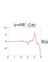
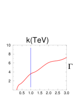
Figure 1: left: Time dependence for a selected mode, $k=0.5T$ with $m=4$ TeV, $\sigma=5T$, $T=1$ TeV and $\Lambda=30$. The function is periodic with exponentially growing amplitude; right: amplification rate $\Gamma$ as a function of the wave number $k$ for the selected set of parameters. Total amplification is exponential in the number of cycles ${\it n}$: ${\cal A}\equiv e^{\Gamma{\it n}}$. To the right of the vertical line $k^{-1}<r_{Debye}$ and our assumption of a neutral plasma is not valid.

4 Implications for Electroweak Baryogenesis

To obtain the average magnetic energy density in amplified fields we have to average over the initial conditions, which may result, for example, from initial thermal or quantum fluctuations. We assume translation and rotation invariance, $\langle B^{\pm}({\vec{k}},\eta){B^{\pm}({\vec{\ell}},\eta)}^{*}\rangle_{|\eta=0}=\delta^{3}({\vec{k}}-{\vec{\ell}})\ \delta_{+-}f^{\pm}(k).$ Using the definition for magnetic power spectrum $P_{B}^{\pm}(k)=4\pi k^{3}f^{\pm}(k),$ the average energy density in amplified fields $\rho_{B}=\frac{1}{8\pi}<B^{2}>$, can be expressed as $\rho_{B}=\frac{1}{8\pi}\int d\ln k$ $\Biggl{\{}P_{B}^{-}(k)\left|{{\cal A}^{-}}({k},\eta)\right|^{2}+P_{B}^{+}(k)\left|{{\cal A}^{+}}({k},\eta)\right|^{2}\Biggr{\}}$, where ${{\cal A}^{\pm}}({k},\eta)$ are the amplification factors for each one of the two magnetic modes.

Since in our case $E_{{\vec{k}}}^{\pm}(\eta)=\pm\frac{1}{k}\partial_{\eta}B_{{\vec{k}}}^{\pm}(\eta)$, and therefore $\langle E^{\pm}({\vec{k}},\eta){B^{\pm}({\vec{\ell}},\eta)}^{*}\rangle=\pm\frac{1}{2}\frac{1}{k}\partial_{\eta}\langle B^{\pm}({\vec{k}},\eta){B^{\pm}({\vec{\ell}},\eta)}^{*}\rangle,$ the CS number density stored in the amplified magnetic modes $\Delta n_{CS}=-\frac{g^{\prime 2}}{4\pi^{2}}\int\limits_{0}^{\eta}d{\widetilde{\eta}}\langle E\cdot B\rangle$, where $g^{\prime}$ is the hypercharge gauge coupling, can be related to $\rho_{B}$

$$n_{CS}=\frac{g^{\prime 2}}{\pi}\int d\ln k\frac{1}{k}\rho_{B}(k)\frac{\gamma^{B}_{AS}+\gamma^{\phi}_{AS}}{1+\gamma^{B}_{AS}\gamma^{\phi}_{AS}},$$ (6)

introducing the asymmetry parameters, ${\gamma}^{B}_{AS}=\frac{P_{B}^{-}(k)-P_{B}^{+}(k)}{P_{B}^{-}(k)+P_{B}^{+}(k)},$  and $\gamma^{\phi}_{AS}=\frac{\left|{{\cal A}^{-}}({k},\eta)\right|^{2}-\left|{{\cal A}^{+}}({k},\eta)\right|^{2}}{\left|{{\cal A}^{-}}({k},\eta)\right|^{2}+\left|{{\cal A}^{+}}({k},\eta)\right|^{2}}.$ Further, we can relate the fractional energy density in coherent magnetic field configurations $\Omega_{B}(k)=\rho_{B}(k)/\rho_{c}$ to the CS fractional number density $n_{CS}/s$, assuming the universe is radiation dominated and the amplification factors ${{\cal A}^{\pm}}_{k}$ are, as we have seen, sharp functions of $k$, peaked at $k_{max}$,

$$\frac{n_{CS}}{s}\simeq 0.01\frac{T}{k_{max}}\Omega_{B}(k_{max})\frac{\gamma^{B}_{AS}+\gamma^{\phi}_{AS}}{1+\gamma^{B}_{AS}\gamma^{\phi}_{AS}}(k_{max}).$$ (7)

This Chern-Simons number will be released in the form of fermions which will not be erased if the EW transition is strongly first order[2], and will generate a baryon asymmetry [3], $\frac{n_{B}}{s}=-\frac{3}{2}\frac{n_{CS}}{s}$. An equal lepton number would also be generated by the same mechanism so that $B-L$ is conserved. Note that the fact that baryon number asymmetry is generated at $k_{max}\neq 0$ does not mean that baryon density is actually inhomogeneous on this short length scale $L_{max}\sim 1/k_{max}$. Comoving neutron diffusion distance at the beginning of nucleosynthesis is much longer than $L_{max}$, so that by that time inhomogeneities would have been erased by free streaming [10]. If $T/k_{max}$ is not too different than unity, as we have seen for the case of oscillating field, and $\gamma^{B}_{AS}$ and $\gamma^{\phi}_{AS}$ are small, it is possible to obtain $\frac{n_{B}}{s}\sim 10^{-10}$ and have strong magnetic fields $\Omega_{B}\sim 1$ present during the EW transition. If $T/k_{max}$ is large and $\gamma^{\phi}_{AS}$ is order unity as we have seen in the rolling case, it is not possible to have strong magnetic fields without producing too many baryons.

5 Experimental Signatures of HyperAxions in Colliders

A pseudoscalar field that couples to hypercharge topological number density as we have described, could be produced and detected in colliders [9]. Since the hypercharge photon is a linear combination of the ordinary photon and the $Z$, the hypothetical particle could be produced, in hadronic or leptonic colliders, in association with photons or $Z$’s through the channels $f\overline{f}\rightarrow Z^{*},\gamma^{*}\rightarrow ZX$ and $f\overline{f}\rightarrow Z^{*},\gamma^{*}\rightarrow\gamma X$, (here $Z^{*}$ and $\gamma^{*}$ denote a virtual $Z$ and a virtual photon, and $f$ is a charged fermion). The produced particle would decay into two neutral gauge bosons, $\gamma\gamma$, $\gamma Z$ or $ZZ$. The experimental signature of these processes would , then, be a triplet of neutral gauge bosons produced in well defined ratios. The almost isotropic angular distribution of momenta of the outgoing bosons could help in separating it from the QED background, that is strongly peaked in the forward/backward directions.

In the simple case of a singlet elementary pseudoscalar whose only coupling to SM fields is to hypercharge topological density, the extra field can be described by two parameters with units of mass: the mass, $m$, and the inverse coupling, $M=1/\lambda$. The plots in Fig. 2 show our estimation of the regions of the $(m,M)$ parameter space where the particle signature could be separated from the background, and so the particle can be detected in present or future colliders. Below the curves, a sufficient number of events to allow detection are expected. Since the particle has not been detected yet, the first plot, that corresponds to LEPII and RunI of the Tevatron, can be used to rule out an interesting region of parameters. In future colliders detection capabilities will be increased significatively in the range of parameters relevant for baryogenesis, as shown in Fig 2.

       

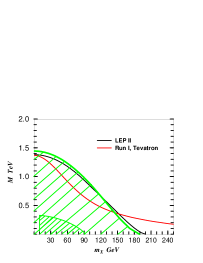
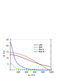
Figure 2: Expected number of HCA’s in present and future colliders. The curves correspond to 10 expected events required for the signal to be distinguished from the SM background. The shadowed region is experimentally ruled out.

References

References

- [1] A. D. Sakharov, Pisma Zh. Eksp. Teor. Fiz. 5 (1967) 32.
- [2] M. E. Shaposhnikov, JETP Lett. 44 (1986) 465.
- [3] M. Giovannini and M. E. Shaposhnikov, Phys. Rev. D57 (1998) 2186.
- [4] P. Elmfors, K. Enqvist, K. Kainulainen, Phys. Lett. B440 (1998) 269.
- [5] D. Grasso, hep-ph/0002197.
- [6] R. Brustein and D. H. Oaknin, Phys. Rev. Lett. 82 (1999) 2628.
- [7] R. Brustein and D. H. Oaknin, Phys. Rev. D60 (1999) 023508.
- [8] E. I. Guendelman and D. A. Owen, Phys. Lett. B276 (1992) 108.
- [9] R. Brustein and D. H. Oaknin, hep-ph/9906344.
- [10] K. Jedamzik and G. M. Fuller, Astrophys. J. 423 (1994) 33.