Contents

toc

I The mSUGRA Paradigm

I.1 Introduction

The purpose of this report is to carry out a study of the prospects for testing mSUGRA at the upgraded Tevatron. It updates the previous studyamidei , taking account of new developments since that report. This study is self contained, including a description of the model, analyses of mSUGRA predictions and a discussion of the prospects for the observation of the signals predicted by the model at the upgraded Tevatron.

The Standard Model of the electro-weak and the strong interactions is experimentally very successful. However, the model is theoretically unsatisfactory. The unsatisfactory nature of the model arises in part due to the existence of 19 arbitrary parameters, the fact that the electro-weak symmetry breaking is accomplished in an ad hoc fashion by the introduction of a tachyonic Higgs mass term in the theory, i.e., $V_{H}=-m^{2}H^{\dagger}H$, and the fact that it suffers from a serious fine-tuning problem. The origin of the gauge heirarchy problem resides in the loop correction to the Higgs boson mass which is quadratically divergent requiring a cutoff $\Lambda$, i.e., $m_{H}^{2}$=$2m^{2}$+ $c\Lambda^{2}$, where $c$ is a constant. The cutoff represents the scale where new physics occurs. If the Standard Model were valid all the way up to the GUT scale without any intervening new physics, then $\Lambda=M_{G}$. In this case the electro-weak scale will be driven to the GUT scale, which is obviously wrong. An alternative procedure would be to arrange the Higgs mass in the electro-weak region by a cancellations between the $m^{2}$ and the $\Lambda^{2}$ terms. However, such a cancellation requires a fine tuning to 22 decimal places, which is highly unnatural. This is a very strong theoretical hint for the existence of new physics beyond the Standard Model. Indeed, requiring no fine-tuning already argues for the existence of new physics in the TeV region.

Supersymmetry offers a very attractive cure for the fine-tuning problem by generating another loop contribution, so that the sum of the loop contributions is free of quadratic divergence. Supersymmetry is a symmetry which connects bosons and fermions, and its multiplets contain bose and fermi helicity states in equal numbers. [In supersymmetry, the Higgs fields have additional interactions involving for example squark loops which also produce a quadratic divergence, cancelling the quadratic divergence from the quark loops and leaving a cutoff dependence of the form ($m_{\tilde{q}}^{2}-m_{q}^{2}$) ln($\Lambda^{2}/m_{\tilde{q}}^{2}$). One finds then that the fine tuning problem can be avoided if the squark masses are in the TeV region.]

The field content of the minimal supersymmetric extension of the Standard Model with the $SU(3)_{C}\times SU(2)_{L}\times U(1)_{Y}$ gauge invariance consists of three generations of quarks, two Higgs doublets $H_{1},H_{2}$ (to give tree-level masses to the up quarks and to the down quarks and leptons and cancel gauge anomalies) and the $SU(3)_{C}\times SU(2)_{L}\times U(1)_{Y}$ gauge bosons, and all their superpartnershaber . Supersymmetry, if it exists, of course, would not be an exact symmetry of nature, as we do not see squarks which are degenerate with the quarks. One possibility is to break supersymmetry by adding soft breaking terms by hand. The number of soft terms one can add is enormous: 105 such terms can be added, making the theory very unpredictive and phenomenologically intractable.

I.2 Model Description

Supergravity unification provides a framework for the spontaneous breaking of supersymmetry, allowing at the same time a cancellation (not fine-tuning) of the cosmological constant, because the potential of the theory is not positive definite. We consider now a class of supergravity grand unified modelscan where the above mechanism of supersymmetry breaking is used to break the degeneracy of the quark and squark masses, etc., in the physical sector of the theory. The basic elements of this procedure consist of breaking supersymmetry in the hidden sector of the theory and communicating this breaking via gravitational interactions to the physical sector of the theory. Thus, one writes the total superpotential of the theory so that $\tilde{W}(z_{i})=W_{h}(z)+W(z_{a})$, where $W_{h}$ is the superpotential that depends on the hidden sector fields $z$, and $W$ depends on the fields $z_{a}$ in the visible sector. The simplest possibility for the breaking of supersymmetry in the hidden sector is via the superHiggs mechanism where one assumes, for example, that $W_{h}$ has the form $W_{h}=m^{2}(z+B)$, where $z$ is a gauge singlet field and $m^{2}$ and $B$ are constants. Minimization of the supergravity potential leads to spontaneous breaking of supersymmetry, with the gravitino developing a mass of ${\cal O}(\kappa m^{2}$) (where $\kappa^{-1}$$\equiv M_{Pl}$ =$(8\pi G_{N})^{-1/2}$= $2.4\times 10^{18}$ GeV), while the graviton remains massless. As will be seen later, soft SUSY breaking masses characterized by the scale $M_{s}\equiv\kappa m^{2}$ lead to spontaneous breaking of the electro-weak symmetry, producing the connectioncan ; applied

$$M_{s}={\cal O}(1)\rm~{}TeV$$ (1)

An alternative mechanism for the breaking of supersymmetry is by gaugino condensation arising from $m_{C}^{3}\equiv\left<\lambda\gamma^{0}\lambda\right>\neq 0$, which gives the soft SUSY breaking scale $M_{s}\sim\kappa^{2}\left<\lambda\gamma^{0}\lambda\right>\neq 0$. Here $M_{s}\sim{\cal O}$(1TeV) requires that $m_{C}\sim 10^{12-13}$ GeV. This mechanism is more difficult to implement explicitly, because gaugino condensation is a non-perturbative phenomenon. The fact that there are no interactions except gravitational between the hidden sector fields and the fields of the visible sector protect the visible sector from mass growth of size $\left<z\right>={\cal O}(M_{Pl}$), which can ruin the mass hierarchy of the theory. Also included in the mSUGRA model is a new multiplicative-conserved symmetry called $R$-parity, which can be written $R_{P}(-1)^{3B+L+2S}$, and which serves to prevent the rapid decay of the proton via SUSY-mediated interactions.

We consider now models which satisfy the following conditions: (i) SUSY breaks in the hidden sector via a super Higgs or gaugino condensation, (ii) The symmetry of the GUT sector breaks so that the GUT gauge group G$\rightarrow SU(3)_{C}\times SU(2)_{L}\times U(1)_{Y}$ at the scale $M_{G}$, (iii) The Kähler potential has no generational dependent couplings with the super Higgs field. Under these assumptions, integration of the super Higgs fields and of the superheavy fields gives an effective potential in the low energy regime, so that $V_{SB}$=$m_{0}^{2}$ $z_{a}z_{a}^{\dagger}$+ ($A_{0}W^{(3)}$+$B_{0}W^{(2)}$+h.c.), where $W=W^{(2)}+W^{(3)}$, with $W^{(2)}$ and $W^{(3)}$ being the quadratic and cubic part of the observable sector superpotential. Additionally, one has a universal gaugino mass term of the form $L_{mass}^{\lambda}=-m_{1/2}\bar{\lambda}\lambda$. The effective theory below the GUT scale $M_{G}$ contains four soft breaking parameters: these are the universal scalar mass $m_{0}$, the universal gaugino mass $m_{1/2}$, and the universal scaling factors $A_{0}$ and $B_{0}$ of the cubic and quadratic couplings. In addition, there is one more parameter in the theory, the Higgs mixing parameter $\mu_{0}$, which appears in $W^{(2)}$ =$\mu_{0}H_{1}H_{2}$. Although $\mu_{0}$ is not a soft SUSY breaking parameter its origin may be linked to soft SUSY breaking. One way to see the origin of this term is to note that the $H_{1}H_{2}$ term can naturally appear in the Kähler potential as it is a dimension two operator. One can use the Kähler transformation to move this term from the Kähler potential to the superpotential. A value $\mu_{0}\sim M_{s}$ then naturally arises after spontaneous breaking of supersymmetry. The mSUGRA model at the GUT scale is then characterized by the five parameters, $m_{0},m_{1/2},A_{0},B_{0},\mu_{0}$. An essential feature of mSUGRA iscan that the soft breaking sector is protected against mass growths proportional to $M_{G}^{2}/M_{Pl}$, $M_{G}^{3}/M_{Pl}^{2}$,…, which all cancel in the low energy theory.

One of the remarkable aspects of mSUGRA is that it leads to the radiative breaking of the $SU(2)_{L}\times U(1)$ symmetry as a consequence of renormalization group effectsewb ; ross . As one evolves the soft SUSY breaking parameters from the GUT scale towards the electro-weak scale the determinant of the Higgs mass matrix in the Higgs potential turns negative generating spontaneous breaking of the electro-weak symmetry. Minimization of the potential including loop corrections allows one to compute the two Higgs VEV’s $v_{1}=\left<H_{1}\right>$ and $v_{2}=\left<H_{2}\right>$ in terms of the parameters of the theory. Alternately, one can use the minimization equations to eliminate the parameter $\mu$, where $\mu$ is the value of $\mu_{0}$ at the electro-weak scale, in terms of the Z boson mass, and eliminate the parameter $B_{0}$ in terms of tan$\beta\equiv v_{2}/v_{1}$. Including radiative breaking of the electroweak symmetry mSUGRA can be characterized by four parameters and the sign of $\mu$

$$m_{0},m_{1/2},A_{0},\tan\beta,~{}\rm sign(\mu)$$ (2)

There are 32 supersymmetric particles in the theory whose masses are determined in terms of the four parameters of the theoryross . We list these particles in Table 1. Our notation is defined in the following section.

Table 1: List of physical states.

particle name	symbol	spin
gluino	$\tilde{g}$	1/2
charginos	$\tilde{\chi}_{1}^{\pm}$, $\tilde{\chi}_{2}^{\pm}$	1/2
neutralinos	$\tilde{\chi}_{1}^{0}$, $\tilde{\chi}_{2}^{0}$, $\tilde{\chi}_{3}^{0}$, $\tilde{\chi}_{4}^{0}$	1/2
sleptons	$\tilde{e}_{L}$, $\tilde{\nu}_{e_{L}}$, $\tilde{e}_{R}$	0
	$\tilde{\mu}_{L}$, $\tilde{\nu}_{\mu_{L}}$, $\tilde{\mu}_{R}$	0
	$\tilde{\tau}_{1}$,$\tilde{\tau}_{2}$, $\tilde{\nu}_{\tau_{L}}$	0
squarks	$\tilde{u}_{L}$, $\tilde{d}_{L}$, $\tilde{u}_{R}$,$\tilde{d}_{R}$	0
	$\tilde{c}_{L}$,$\tilde{s}_{L}$, $\tilde{c}_{R}$,$\tilde{s}_{R}$	0
	$\tilde{t}_{1}$, $\tilde{t}_{2}$, $\tilde{b}_{1}$,$\tilde{b}_{2}$	0
higgs	h, H, A, $H^{\pm}$	0

Thus many sum rules exist among the mSUGRA mass spectrum which are experimentally testable. An interesting property of radiative breaking is that over most of the parameter space of the theory one finds that $\mu^{2}/M_{Z}^{2}\gg 1$ and this leads to the approximate relations

$$2m_{\tilde{\chi}_{1}}^{0} \cong m_{\tilde{\chi}_{1}}^{\pm}\cong m_{\tilde{\chi}_{2}}^{0}\simeq{1\over 3}m_{\tilde{g}}$$

$$m_{\tilde{\chi}_{3}}^{0} \cong m_{\tilde{\chi}_{4}}^{0}\cong m_{\tilde{\chi}_{2}}^{\pm}\simeq|\mu|\gg m_{\tilde{\chi}_{1}}^{0}$$ (3)

The above implies that the light neutralino and chargino states are mostly gauginos, and the heavy states mostly higgsinos. It also turns out that under the constraints of electro-weak symmetry breaking the lightest neutralino is also the lightest mass supersymmetric particle (LSP) over most of the parameter space of the theory.

An interesting aspect of mSUGRA model is that it automatically includes a super GIM mechanism for the suppression of flavor changing neutral currents for the process $K_{L}\rightarrow\mu^{+}\mu^{-}$. The mSUGRA boundary conditions give the following relation

$$m_{\tilde{c}}^{2}-m_{\tilde{u}}^{2}=m_{c}^{2}-m_{u}^{2}$$ (4)

The super GIM suppression occurs because the squark loop contributions in the process $K_{L}\rightarrow\mu^{+}\mu^{-}$ enter in the combination $m_{\tilde{c}}^{2}-m_{\tilde{u}}^{2}$ which because of Eq. (5) is suppressed. The degeneracy of the squark masses necessary for the super GIM to work is enforced by the universality condition of Eq. (3). The universality of the gaugino masses at the GUT scale, which is enforced in any case when the $SU(3)_{C}\times SU(2)_{L}\times U(1)_{Y}$ gauge group is embedded in a simple GUT group, obey the following one loop relation at scales below the GUT scale

$$M_{i}=m_{1/2}\frac{\alpha_{i}}{\alpha_{G}}$$ (5)

where i=1,2,3 for $U(1)_{Y}$, $SU(2)_{L}$, $SU(3)_{C}$, $\alpha_{i}$ is the $i^{\rm th}$ fine structure constant, and $\alpha_{G}=\alpha_{i}(M_{G})$ is the GUT scale coupling constant. Note that $\alpha_{1}={5\over 3}\alpha^{\prime}$, where $\alpha^{\prime}$ is the Standard Model hypercharge fine structure constant. There are, however, important 2 loop QCD contributions for the case i=3mart . The high precision LEP data on the gauge coupling constants at the Z scale, i.e., $\alpha_{i}(M_{Z})$alpha and the experimental ratio of $m_{b}/m_{\tau}$bbo appear to be consistent with ideas of SUSY and mSUGRA unification.

In investigating the parameter space of mSUGRA one uses somewhat subjective naturalness constraints on the soft SUSY parameters. The simplest approach is to set

$$m_{0},~{}m_{\tilde{g}}\leq 1~{}TeV\,;$$ (6)

more sophisticated approaches have also been discussed. For studies of physics at the Tevatron, the naturalness assumption of Eq. (6) appears sufficient. However, the constraint of Eq. (6) must be revised upwards for analyses at the LHC which can probe higher regions of the mSUGRA parameter space. In investigating the implications of mSUGRA one must also impose additional experimental constraints such as those from (i) $b\rightarrow s+\gamma$ decay and from (ii) the value of $g_{\mu}-2$.

Constraint (i) arises from the experimental limit on $b\rightarrow s+\gamma$ from CLEOcleo , which gives BR($b\rightarrow s+\gamma$) =(3.15$\pm 0.54$)$\times 10^{-4}$, and ALEPHaleph-nath , which gives $(3.11\pm 0.80_{\rm stat}\pm 0.72_{\rm syst})\times 10^{-4}$. This decay receives contributions in the Standard Model from $W$ boson exchange. Here, recent analysesburas , including the leading and the next to leading order QCD corrections and two-loop electroweak corrections, give the branching ratio BR($b\rightarrow s+\gamma$) =(3.32$\pm 0.29$)$\times 10^{-4}$. In mSUGRA, there are additional contributions from the exchange of the charged Higgs, the charginos, the gluinos, and the neutralinosbert . While the exchange of the charged Higgs gives a constructive intereference with SM amplitudes, the exchange of the charginos and the neutralinos can give contributions with either signhewett . The experimental $b\rightarrow s+\gamma$ branching ratio puts a stringent constraint on the parameter space of the theory. As will be discussed later the $b\rightarrow s+\gamma$ constraint affects in a very significant way dark matter analyses for one sign of $\mu$na . A further reduction of the experimental error in this decay mode will certainly constrain the parameter space further and may even reveal the existence of new physics if a significant deviation from the SM results are confirmed.

Constraint (ii) is relevant because supersymmetric contributions to ($g_{\mu}-2$) can be very significantkosower . The current experimental value of $a_{\mu}\equiv(g_{\mu}/2-1)$ is $a_{\mu}^{exp}=1.1659230(84)\times 10^{-10}$ while the Standard Model result for $a_{\mu}$ is given by $a_{\mu}^{theory}(SM)=11659162.8(7.7)\times 10^{-10}$davier . In mSUGRA, additional contributions to $(g-2)$ arise from the exchange of the charginos and the neutralinos. One finds that the supersymmetric electro-weak contributions can be as large or even larger than the Standard Model electro-weak contributions. In fact, supersymmetric contributions can be large enough that even the current experiment puts a constraint on the mSUGRA parameter space. In the near future, the Brookhaven experiment E821 will begin collecting data and is expected to increase the sensitivity of the ($g_{\mu}-2$) measurement by a factor of 20, to $a_{\mu}\sim 4\times 10^{-10}$. The improved measurement may reveal the existence of new physics beyond the Standard Model, or if no effect is seen, would constrain the mSUGRA parameter space even further. In either case, the (g${}_{\mu}-2$) experiment is an important test of mSUGRA.

We can supplement the mSUGRA analysis with further contraints which involve additional assumptions. Thus, for example, we can consider the constraints of

• (iii) relic density

• (iv) $b-\tau$ unification

• (v) proton lifetime limits

Constraint (iii) applies when $R$-parity is conserved. This possibility is very attractive, in that in this case the lightest neutralino becomes a candidate for cold dark matter (CDM) over much of the parameter space of the model. Currently there exists a whole array of cosmological models such as HCDM, $\Lambda$CDM, $\Lambda$HCDM, $\tau$CDM,…etc., which all require some component of CDM. At the very minimum one has the constraint that the supersymmetric dark matter not overclose the universe, i.e., $\Omega_{\tilde{\chi}_{1}}^{0}<1$, where $\Omega=\rho_{\tilde{\chi}_{1}^{0}}/\rho_{c}$, where $\rho_{\tilde{\chi}_{1}^{0}}$ is the neutralino matter density and $\rho_{c}$ is the critical matter density needed to close the universe. Of course, more stringent constraints on $\Omega_{\tilde{\chi}_{1}}^{0}h^{2}$, which is the quantity computed theoretically (where $h$ is the Hubble parameter in units of 100km/sec Mpc.) would ensue if one assumed a specific cosmological modelrelic . The density contraints can be very severe in limiting the parameter space of mSUGRA. These results have also important implications for the search for dark matterdetection . Constaints (iv) and (v) are more model-dependent as compared to the constraints (i)–(iii). Thus, for example, the predictions of $m_{b}/m_{\tau}$ mass ratio depends on the GUT group and on the texturesbbo . Similarly, the nature of the GUT group and textures also enter in the analysis of proton lifetimepdecay . It should be noted that a tiny amount of $R$-parity violation at a level irrelevant for collider searches could negate any constraints from the cosmological relic density.

I.3 Extensions of mSUGRA

We discuss now some possible generalizations of mSUGRA.

• (a) CP violation

• (b) Non-universalities of soft terms

• (c) R parity violation

• (d) Corrections from Planck scale physics

• (e) Connection of mSUGRA to M theory

We discuss briefly each of these items and more discussion will follow in the subparts later.

(a) The mSUGRA formalism allows for complex phases for the soft parameters. However, not all the phases are independent. One can remove all but two phases, which can be chosen to be $\theta_{\mu_{0}}$ (the phase of $\mu_{0}$) and $\alpha_{A_{0}}$ (the phase of $A_{0}$), so that the mSUGRA parameter space with CP violation expands to six parameters, i.e., Eq. (2) is replaced by

$$m_{0},m_{1/2},A_{0},tan\beta,\theta_{\mu_{0}},\alpha_{A_{0}}\,.$$ (7)

One of the important constraints on SUSY models with CP violation arises from the experimental limits on the neutron edm and on the electron edm. The current experimental limits on these are $d_{n}<1.1\times 10^{-25}$e$\cdot$cm for the neutron, and $d_{e}<4.3\times 10^{-27}$e$\cdot$cm for the electron. These limits produce a strong constraint on the parameter space of Eq. (7)cp .

(b) As mentioned earlier, the universality of the scalar soft breaking terms arises from the assumption that the Kähler potential does not have generational dependent couplings with the hidden sector fields. A relaxation of this constraint leads to non-universalities of the soft breaking termssoni , which must then be restricted by group symmetries and the phenomenological constraints of flavor changing neutral currents (FCNC). One of the sectors which is not very strongly constrained by FCNC is the Higgs sector, and one can introduce non-universalities of the type

$$m_{H_{1}}^{2}(M_{G})=m_{0}^{2}(1+\delta_{1}),~{}m_{H_{2}}^{2}(M_{G})=m_{0}^{2}(1+\delta_{2})$$ (8)

where the typical range considered for the $\delta_{i}$ is $|\delta_{i}|\leq 1$. Similarly, FCNC constraints are also insensitive to the non-universalities in the third generation sector and one may consider non-univesralities in this sector along with the non-universalities in the Higgs sector. The non-universalities produce identifiable signals at low energysoni .

(c) Analysis of signatures of supersymmetry in mSUGRA depend importantly on whether or not one assumes $R$-parity invariance. If one assumes that $R$-parity is conserved, then the LSP is stable and one will have supersymmetric particle decays which result in lots of missing energy. If $R$-parity is violated, then the LSP is not stable and will decay with possible signatures of 2 charged leptons ($l_{i}l_{j}\nu_{k}$), lepton and 2 jets ($l_{i}u_{j}\bar{d}_{k}$, $\nu_{i}d_{j}\bar{d}_{k}$), and three jets ($d_{i}d_{j}u_{k}$). Thus the signatures of SUSY events at colliders would be very different if $R$-parity is violatedrparity .

(d) There can be important corrections to mSUGRA predictions from Planck scale termsplanck . This possibility arises because $M_{G}$ is only two 1–2 orders of magnitude away from the string/Planck scale and thus corrections of O($M_{G}/M_{Pl}$) could be relevant. One example of such corrections is the Planck contribution to the gauge kinetic energy function $f_{\alpha\beta}$ which produces splittings of the $SU(3)_{C}$, $SU(2)_{L}$, and $U(1)_{Y}$ gauge couplings at the GUT scale. The same Planck correction can generate non-universal contributions to the gaugino masses at the GUT scale. Planck corrections may also be responsible for the generation of textures which control the hierarchy of quark-lepton masses at low energy.

(e) Although currently one does not have a phenomenologically viable string model, it is our hope that such a model exists and that perhaps mSUGRA is its low energy limit below the string scale $M_{str}\approx 5\times 10^{17}$ GeV. The underlying structure of mSUGRA, i.e., N=1 supergravity coupled to matter and gauge fields, is what one expects in the low energy limit of a compactified string model. It is also possible to envision how the soft breaking sector of mSUGRA can arise in strings where the fields governing SUSY breaking are the dilaton (S) and the moduli ($T_{i},\bar{T}_{i}$). Of course, the problem of SUSY breaking in string theory is as yet unsolved, and consequently one cannot make serious predictions either in the weakly coupled heterotic string or in its strongly coupled M-theory limit. However, when one has a viable string model with the right SUSY breaking, it would be possible to make connection with mSUGRA at the string scale by matching the boundary conditions at $M_{str}$.

Other extensions beyond (a)–(e) are discussed elsewhere in this volume.

I.4 Signals of supersymmetry in mSUGRA

Aside from indirect signals that might appear in the precision experimental determination of $b\rightarrow s+\gamma$ and in the $g_{\mu}-2$ measurements, one can have signals via decay of the proton and via the direct detection of a neutralino in dark matter detectors. However, the most convincing evidence of supersymmetry will be the direct observation of supersymmetric particles at colliders. The purpose of this report is to study the reach of the upgradraded Tevatron for SUSY particles in various channels. One of the signals is the production of the Higgs in direct collisions, i.e., $q\bar{q},gg\rightarrow$ $h,H,A,H^{\pm}$. The tree level mass of the lightest Higgs is governed by gauge interactions, with important modifications arising from one- and two-loop corrections. Generally, one expects $m_{h}$ to obeyhiggs

$$m_{h}\leq 120\mbox{--}150\rm\ GeV$$ (9)

The upper limit on the Higgs is somewhat model dependent because the soft parameters enter in the loop corrections to the Higgs mass. However, Eq.(9) represents a fair upper limit on $m_{h}$ for any reasonable naturalness assumption on $m_{0}$ and $m_{1/2}$. The upper limit on the Higgs mass is lowered if one includes additional constraints discussed earlier. There are several processes which give pair production of sparticles at hadron colliders. Thus, squarks and gluinos can be pair produced via processes such as $q\bar{q}$, $qg$, $gg$ $\rightarrow\tilde{q}\bar{\tilde{q}}$, ${\tilde{q}}{\tilde{g}}$, ${\tilde{g}}{\tilde{g}}$. Similarly, one can have pair production of chargino and neutralino final states, i.e., $\tilde{\chi}_{i}^{\pm}\tilde{\chi}_{j}^{\mp}$, $\tilde{\chi}_{i}^{\pm}\tilde{\chi}_{j}^{0}$, $\tilde{\chi}_{i}^{0}\tilde{\chi}_{j}^{0}$ as well as final states such as $\tilde{q}\tilde{\chi}_{i}^{\pm}$, $\tilde{g}\tilde{\chi}_{i}^{\pm}$, $\tilde{q}\tilde{\chi}_{i}^{0}$, $\tilde{g}\tilde{\chi}_{i}^{0}$. Other SUSY states that can be pair produced are $\tilde{l}\tilde{l}$, $\tilde{l}\tilde{\nu}$, $\tilde{\nu}\tilde{\nu}$.

With $R$-parity invariance, sparticles must decay to other sparticles until this decay chain terminates in the neutral stable LSP which escapes detection. Typical SUSY signals all involve large missing energy events with the neutralinos and neutrinos carrying the missing energy. For instance, the chargino decay involves

$$\tilde{\chi}_{1}^{-}\rightarrow e^{-}\bar{\nu}\tilde{\chi}_{1}^{0}$$ (10)

which exhibits the signature $e^{-}+E_{T}$(missing) in the final state. Similarly, the decay of the squark involves $\tilde{q}\rightarrow$ $q+\tilde{\chi}_{1}^{0}$ as one of its modes which in the final state will give jet+$E_{T}$(missing). A signal of particular interest is the trileptonic signal, which arises from the decay of the final states $\tilde{\chi}_{1}^{\pm}\tilde{\chi}_{2}^{0}$ via the channels $\tilde{\chi}_{1}^{\pm}\rightarrow$ $l\nu\tilde{\chi}_{1}^{0}$ and $\tilde{\chi}_{2}^{0}\rightarrow l\bar{l}\tilde{\chi}_{1}^{0}$. In this case one finds $\bar{l}_{1}l_{1}l_{2}+E_{T}$(missing). This channel is fairly clean, with no hadronic activity expected from QCD radiations, and is thus a promising channel for the detection of supersymmetry.

II Status of Unification of Couplings in the MSSM

Although the Minimal Supersymmetric extension of the Standard Model (MSSM) enables a natural solution to the hierarchy problem of the Standard Model (SM), it is thought to provide only a low energy effective description of a more fundamental, unified, theory which will become manifest at much higher energy scales. One of the possible experimental tests of this framework is the unification of the renormalization group evolved gauge couplings. The scale at which the couplings unify gives a hint of the relevant energy at which the low energy description should be replaced by the more fundamental one. The condition of unification gut ; unif is a non-trivial one, since it depends on the exact relation between the $\beta$ function coefficients and on the low energy values of the three gauge couplings measured experimentally. The idea of unification can be tested quantitatively, but it is always associated with large theoretical uncertainties, related to the unknown spectrum of supersymmetric particles at low energies, as well as the exact physical thresholds at scales close to the grand unification scale. A possible approach to treat these uncertainties is to develop a bottom-up approach:

1. Obtain the low energy values of the three gauge couplings including the corrections induced by one-loop diagrams of standard model particles and their superpartners.

2. Compute the high energy threshold necessary to achieve the unification of gauge couplings by extrapolating their low energy values to high energies via two-loop renormalization group evolution.

In this approach, one assumes the absence of new physics affecting the evolution of the gauge couplings, up to scales of order of the grand unification scale.

The value of the gauge couplings in the modified $\overline{MS}$ scheme in the Standard Model are well known. The largest uncertainty is associated with the strong gauge coupling, whose value is known only at the level of 3%, $\alpha_{3}(M_{Z})\simeq 0.119\pm.003$ PDB . The values of the weak gauge couplings, instead, are known with high precision. In particular, the value of the weak mixing angle can be given as a function of the electroweak parameters $G_{F}$, $M_{Z}$, $1/\alpha_{em}(M_{Z})(\simeq 127.9$ LP ), the pole top quark mass $M_{t}$ and the Higgs mass $m_{h}$. For a Higgs mass of order of 100 GeV, as is appropriate in low energy supersymmetric models, and a pole top quark mass of order of 170 GeV, $\sin^{2}\theta_{W}(M_{Z})$ in the modified $\overline{MS}$ scheme is given by LP ; CPP ,

$$\sin^{2}\theta_{W}(M_{Z}) \simeq 0.2315+5.4\times 10^{-6}(m_{h}-100)-2.4\times 10^{-8}(m_{h}-100)^{2}$$ (11)

$$-3.\times 10^{-5}(M_{t}-170)-8.4\times 10^{-8}(M_{t}-170)^{2}\pm 0.0003.$$

All the masses are in GeV units. The above expressions take into account all one-loop corrections within the Standard Model.

Supersymmetric one-loop diagrams lead to logarithmic corrections, as well as corrections proportional to the inverse of the supersymmetric particle masses that become negligible when the masses are pushed towards large values with respect to $M_{Z}$. The decoupling of the non-logarithmic corrections is very fast and, within the present experimental limits, these corrections become relevant only if there are light, left-handed doublets which appear in the spectrum. The logarithmic corrections, instead, are very important for obtaining the exact supersymmetric predictions. Their effect can be studied by renormalization group methods, using a step function decoupling of the supersymmetric particle contributions, at energies below the relevant supersymmetric particle mass. This program leads to the following expressions:

$$\frac{1}{\alpha_{i}(M_{G})} = \frac{1}{\alpha_{i}(M_{Z})}-\frac{b_{i}}{2\pi}\ln\left(\frac{M_{G}}{M_{Z}}\right)+\gamma_{i}+\frac{1}{\alpha_{i}^{\rm thr.}}$$

$$\frac{1}{\alpha_{i}^{\rm thr.}} = \sum_{\eta}\frac{b_{i}^{\eta}}{2\pi}\ln\left(\frac{M_{\eta}}{M_{Z}}\right)+{\rm h.e.t.}$$ (12)

where $\gamma_{i}$ represents the two-loop corrections, as well as the corrections factors to convert from the modified $\overline{MS}$ scheme to the $\overline{DR}$ scheme, $M_{G}$ is the scale at which the weak gauge couplings unify, $b_{i}^{\eta}$ is the contribution to the $\beta_{i}$ function coefficient of the superparticle $\eta$ with mass $M_{\eta}$ and h.e.t. denotes the corrections coming from the unknown high energy theory at scales of order of $M_{G}$. Using these equations, a simple formula for the low energy value of the strong gauge coupling can be obtained as a function of the weak gauge couplings under the assumption of exact unification of gauge couplings at the scale $M_{G}$ (i.e., neglecting GUT-scale threshold effects),

$$\frac{1}{\alpha_{3}(M_{Z})}=(1+B)\left[\frac{1}{\alpha_{2}(M_{Z})}+\gamma_{2}\right]-B\left[\frac{1}{\alpha_{1}(M_{Z})}+\gamma_{1}\right]-\gamma_{3}+\frac{1+B}{\alpha_{2}^{{\rm thr.}}}-\frac{B}{\alpha_{1}^{{\rm thr.}}}-\frac{1}{\alpha_{3}^{{\rm thr.}}},$$ (13)

where

$$B=\frac{b_{2}-b_{3}}{b_{1}-b_{2}}.$$ (14)

As mentioned above, the predictions coming from gauge coupling unification depend strongly on the low energy values for the gauge couplings, as well as on the relation between the different $\beta_{i}$ coefficients. As a first test of the unification relations, one can ignore the threshold corrections, as well as the small $\gamma_{i}$ correction factors. One can then deduce the value of $B$ needed in order to obtain a good unification prediction,

$$\left.B\right|_{\rm unif.}=\frac{(\alpha_{2}(M_{Z}))^{-1}-(\alpha_{3}(M_{Z}))^{-1}}{(\alpha_{1}(M_{Z}))^{-1}-(\alpha_{2}(M_{Z}))^{-1}}\simeq 0.7.$$ (15)

In the MSSM, $B=5/7$, leading to an excellent agreement between theory and experiment at the one-loop level.

The above procedure can be extended to include the effect of the threshold of low energy supersymmetric particles. These can be described in terms of one single scale $T_{SUSY}$ LP . Considering different characteristic mass scales for left-handed squarks ($m_{\tilde{Q}}$), right-handed squarks ($m_{\tilde{U}}$), gluinos ($m_{\tilde{g}}$), left-handed sleptons ($m_{\tilde{L}}$), right-handed sleptons ($m_{\tilde{E}}$), electroweak gauginos ($m_{\tilde{W}}$), Higgsinos ($m_{\tilde{H}}$) and the heavy Higgs doublet ($m_{H}$), $T_{SUSY}$ is given as CPW

$$T_{SUSY}=m_{\tilde{H}}\left(\frac{m_{\tilde{W}}}{m_{\tilde{g}}}\right)^{\frac{28}{19}}\left[\left(\frac{m_{H}}{m_{\tilde{H}}}\right)^{\frac{3}{19}}\left(\frac{m_{\tilde{W}}}{m_{\tilde{H}}}\right)^{\frac{4}{19}}\left(\frac{m^{3}_{\tilde{L}}m^{7}_{\tilde{Q}}}{m^{2}_{\tilde{E}}m^{5}_{\tilde{U}}m^{3}_{\tilde{D}}}\right)^{\frac{3}{19}}\right]$$ (16)

Assuming exact unification at the scale $M_{G}$ and ignoring threshold corrections induced by physics at the grand unification scale, the value of the strong gauge coupling at low energies is determined as a function of $\sin^{2}\theta_{W}$, $\alpha_{em}$ and $T_{SUSY}$. The result is

$$\left.\frac{1}{\alpha_{3}(M_{Z})}=\frac{1}{\alpha_{3}(M_{Z})}\right|_{\rm SUSY}+\frac{19}{28\pi}\ln\left(\frac{T_{SUSY}}{M_{Z}}\right),$$ (17)

where $\alpha_{3}(M_{Z})|_{SUSY}$ would be the value of the strong gauge coupling at $M_{Z}$ if the theory were exactly supersymmetric down to the scale $M_{Z}$.

The effective threshold scale $T_{SUSY}$, Eq. (16), has only a mild dependence on the squark and slepton masses. This can be traced to the fact that squarks and sleptons come in complete representations of $SU(5)$ which modify all $\beta_{i}$ coefficients in the same way, keeping the value of $B$ constant. The scale $T_{SUSY}$ depends strongly on the overall Higgsino mass, as well as on the ratio of masses of the weakly and strongly interacting gauginos. In models with universal gaugino masses at the grand unification scale,

$$T_{SUSY}\simeq m_{\tilde{H}}\left(\frac{\alpha_{2}(M_{Z})}{\alpha_{3}(M_{Z})}\right)^{3/2}\simeq\frac{|\mu|}{7}\;,$$ (18)

where $|\mu|$ characterizes the Higgsino mass in the case of negligible mixing in the neutralino/chargino sector. Hence, even if all supersymmetric masses are of the order of 1 TeV, the effective supersymmetric scale $T_{SUSY}$ can still be of the order of the weak scale, or smaller.

It is also interesting to investigate the variation of the scale at which the gauge couplings $\alpha_{1}$ and $\alpha_{2}$ unify as a function of the low energy supersymmetric spectrum. From the above equations, we obtain CPP

$$\left.M_{G}=M_{G}\right|_{SUSY}\times\left(\frac{M_{Z}}{G_{SUSY}}\right)^{2/7}$$ (19)

where

$$G_{SUSY}=\left(M_{H}m_{\tilde{H}}^{4}m_{\tilde{W}}^{20}\right)^{1/25}\times\frac{\left(M_{\tilde{Q}}M_{\tilde{L}}\right)^{1/8}}{\left(M_{\tilde{U}}^{4}M_{\tilde{D}}M_{\tilde{E}}^{3}\right)^{1/8}}$$ (20)

where $\left.M_{G}\right|_{SUSY}$ is the unification scale value that would be obtained if the theory is supersymmetric up to the scale $M_{G}$. Observe that, due to the small value of the exponent in Eq. (19), the grand unification scale is quite stable under variations of the low energy superymmetry breaking mass parameters. In particular, it cannot be reconciled with the string scale in weakly coupled string theory, $M_{S}\simeq 5\times 10^{17}$ GeV by means of $G_{SUSY}$.

For a top quark mass of the order of 170 GeV, assuming that all sparticles are heavy, so that non-logarithmic corrections can be ignored, and ignoring corrections induced by particles with masses of order of $M_{G}$, the unification condition implies the following numerical correlation LP ; Nir2 ; BCPW ,

$$\alpha_{3}(M_{Z})\simeq 0.128+1.2\times 10^{-4}\left(M_{t}[GeV]-170\right)-0.0035\ln\left(\frac{T_{SUSY}}{M_{Z}}\right)$$ (21)

The values quoted above take already into account the negative corrections obtained from a large top Yukawa coupling, like the ones obtained for low values of $\tan\beta\simeq 2$ ($h_{t}(m_{t})\simeq 1.1$ at the weak scale). For moderate values of $\tan\beta\simeq 5$, the value of $\alpha_{3}(M_{Z})$ increases by one percent, due to the slightly lower values of the top quark Yukawa coupling, while for large values of $\tan\beta$ it can decrease by one percent compared to the values given in Table 2, if both the top and the bottom Yukawa coupling become large.

Table 2: Gauge coupling unification predictions for $\alpha_{s}(M_{Z})$, for given values of $\sin^{2}\theta_{W}$ (correlated with $M_{t}$), $m_{h}=M_{Z}$ and $T_{SUSY}=1$ TeV, 400 GeV, and $(M_{Z})$.

$M_{t}$[GeV]	$\sin^{2}\theta_{W}(M_{Z})$	$\alpha_{3}(M_{Z})$	$\alpha_{3}(M_{Z})$	$\alpha_{3}(M_{Z})$
		$T_{SUSY}$ = 1 TeV	$T_{SUSY}=400$ GeV	$T_{SUSY}=M_{Z}$
170	0.2315	0.119	0.123	0.128

The predicted value of $\alpha_{s}(M_{Z})$ from unification may be further modified if some sparticle masses are ${\cal{O}}(M_{Z})$. Indeed, not only the leading-log contributions but the full one-loop threshold contributions from SUSY loops should be included when extracting the couplings from the data CPP ; all ; BMP . The main additional effects come from light sfermions and are given by Nir2 –all

$$\frac{\delta\sin^{2}\theta_{W}}{\sin^{2}\theta_{W}}\simeq\frac{\cos^{2}\theta_{W}}{\sin^{2}\theta_{W}-\cos^{2}\theta_{W}}\left(\frac{\delta\alpha_{em}}{\alpha_{em}}+\frac{\Pi_{WW}(0)}{M_{W}^{2}}-\frac{\Pi_{ZZ}(M_{Z}^{2})}{M_{Z}^{2}}\right),$$ (22)

where $\Pi_{ij}$ are the vacuum polarization contributions to the gauge bosons. The above corrections to $\sin^{2}\theta_{W}$ are dominated by the logarithmic corrections discussed above, which are induced by a correction to the electromagnetic coupling and to the external momentum dependent part of $\Pi_{ZZ}(q^{2})$. For particle masses far from the $Z$-production threshold, the dominant non-logarithmic corrections are approximately described by the parameter $\Delta\rho(0)=\Pi_{WW}(0)/M_{W}^{2}-\Pi_{ZZ}(0)/M_{Z}^{2}$. In the MSSM it follows that $\Delta\rho(0)^{SUSY}\geq 0$ and, after considering the additional terms in Eq. (22), one still obtains that the correction to $\sin^{2}\theta_{W}$ induced by the non-logarithmic corrections $\delta_{\rm non-LL}\sin^{2}\theta_{W}\stackrel{{\scriptstyle<}}{{{}_{\sim}}}0$ in all the parameter space consistent with the present experimental constraints. This translates into an increase, with respect to the results from Table 2, in the values of $\alpha_{3}(M_{Z})$ predicted from supersymmetric grand unification. One should also note that large corrections to $\Delta\rho(0)$ are disfavoured by present experimental data, particularly for large values of the top quark mass $M_{t}\stackrel{{\scriptstyle>}}{{{}_{\sim}}}170$ GeV, ruling out large non-logarithmic corrections to the unification predictions.

Figure 1 shows the predicted value of $\alpha_{3}(M_{Z})$ as a function of $T_{SUSY}$ for the case of a generic minimal supergravity spectrum (Fig. 1a) and for a low energy supersymmetry spectrum that gives a good fit to the precision electroweak measurement data (Fig. 1b). In the minimal supergravity case, there is a strong correlation between the parameter $|\mu|$ (or, equivalently, $T_{SUSY}$, Eq. (18)) and the squark spectrum. This implies that for low values of $T_{SUSY}$ the non-logarithmic correction to $\sin^{2}\theta_{W}$ tend to become large, leading to a departure of the predicted value of $\alpha_{3}(M_{Z})$ with respect to the one obtained in the leading-logarithmic approximation. The lowest values of $T_{SUSY}$ shown in Fig. 1a correspond to values of the sparticle masses close to the present experimental bounds, which tend to worsen the standard model fit to the precision measurement data. In Fig. 1b, instead, a good fit to the precision measurement data is obtained by relaxing the universality assumption and taking large values of the left-handed stop mass parameters, while keeping small values of those for the right-handed stop. The largeness of the left-handed stop mass ensures the smallness of the non-logarithmic stop-induced corrections to $\sin^{2}\theta_{W}$, implying a good agreement between the predicted value of $\alpha_{3}(M_{Z})$ and the one obtained in the leading-log approximation.

It is interesting to observe that the prediction for $\alpha_{3}(M_{Z})$ is in excellent agreement with the experimental values if:

1. The supersymmetric threshold scale is in the range: 400 GeV $\stackrel{{\scriptstyle>}}{{{}_{\sim}}}T_{SUSY}\stackrel{{\scriptstyle>}}{{{}_{\sim}}}37$ eV.

2. Finite, non-logarithmic corrections induced by supersymmetric particle loops are suppressed.

The predicted value of $\alpha_{3}(M_{Z})$ coming from the condition of exact unification of couplings coincides with the experimental central value of $\alpha_{3}(M_{Z})$ for a scale $T_{SUSY}\simeq$ 1 TeV.

Figure 1: Predictions of $\alpha_{3}(M_{Z})$ as a function of the effective scale $T_{SUSY}$ for $M_{t}=175$ GeV and a generic supergravity spectrum (Fig. 1.a), as well as for a superparticle spectrum, which gives a good fit to the precision electroweak measurement data (Fig. 1b), as described in the text. The solid lines represent the prediction for $\alpha_{3}(M_{Z})$ in the leading logarithmic approximation, Eq. (17).

In supergravity models, the low energy values of the supersymmetry breaking parameters may be computed by the knowledge of their boundary conditions at the grand unification scale and their renormalization group equations. Flavor changing neutral currents are efficiently suppressed if sparticles with the same quantum numbers under the standard model gauge group are assumed to obtain equal supersymmetry breaking masses at the GUT scale. For small or moderate values of $\tan\beta$, assuming that no other particles affect the evolution of the gauge couplings, and taking $\alpha_{3}(M_{Z})=0.12$, the masses at the weak scale are approximately given by five  :

$$M_{i} \simeq \frac{M_{i}(0)}{\alpha_{i}(0)}\alpha_{i}$$

$$m_{\tilde{f}_{i}}^{2} \simeq m_{\tilde{f}_{i}}^{2}(0)\left[1-\frac{y_{t}}{6}(\delta_{Q_{3},i}+2\delta_{U_{3},i})\left(m_{Q}^{2}(0)+m_{U}^{2}(0)+m_{H_{2}}^{2}(0)\right)\right]$$

$$+0.78\;n^{3}_{f_{i}}M_{3}^{2}+0.88\;n_{2}^{f_{i}}M_{2}^{2}+\frac{y_{f_{i}}^{2}}{4}1.55M_{1}^{2}-\Delta m^{2}(M_{i},y_{t})\left(\frac{\delta_{Q_{3},i}}{6}+\frac{\delta_{U_{3},i}}{3}\right)$$

$$m_{H_{i}}^{2} = m_{H_{i}}^{2}(0)\left[1-\frac{y_{t}}{2}\delta_{i,2}\left(m_{Q}^{2}(0)+m_{U}^{2}(0)+m_{H_{2}}^{2}(0)\right)\right]+0.8M_{2}^{2}+0.23M_{1}^{2}-\delta_{i,2}\frac{\Delta m^{2}(M_{i},y_{t})}{2},$$ (23)

where $M_{i}$, with $i=1$–3, are the three gaugino masses at the weak scale, $n^{N}_{f_{i}}$ is equal to 1 if the particle $f_{i}$ belongs to the fundamental representation of $SU(N)$ and is zero otherwise, $y_{f_{i}}^{2}/4=3/5(q_{i}-T_{3})^{2}$, $q_{i}$ is the electric charge of the particle $f_{i}$, $Q_{3}$ and $U_{3}$ denote the third generation squark $SU(2)$ doublet and up squark $SU(2)$ singlet, respectively, and $y_{t}$ denote the square of the ratio of the top quark yukawa coupling to its fixed point value. In the above, a vanishing argument always implies a function evaluated at the grand unification scale. The function $\Delta m^{2}(M_{i},y_{t})$ is given by

$$\Delta m^{2}(M_{i},y_{t}) \simeq y_{t}\left(1.25M_{3}^{2}+1.46M_{2}^{2}+0.6M_{1}^{2}+0.8M_{3}M_{2}+0.23M_{3}M_{1}+0.18M_{2}M_{1}\right)$$ (24)

$$-y_{t}^{2}\left(0.65M_{3}+0.5M_{2}+0.16M_{1}\right)^{2}-y_{t}\left(1-y_{t}\right)A_{0}\left(0.32M_{1}+M_{2}+1.29M_{3}-A_{0}\right)$$

where $A_{0}$ is the stop-Higgs trilinear coupling at the unification scale, and, for convenience, we have written all gaugino factors as a function of their values at the weak scale. The low energy value of the stop-Higgs trilinear coupling $A_{t}$ is given by

$$A_{t}=A_{0}(1-y_{t})-1.15M_{3}-0.8M_{2}-0.16M_{1}+y_{t}\left(0.65M_{3}-0.5M_{2}-0.16M_{1}\right)$$ (25)

Observe that no unification assumption or relation between the high energy values of the soft supersymmetry breaking parameters has been made in the above formulae. The formulae, however, lose their validity for large values of $\tan\beta$, at which the bottom- and $\tau$-Yukawa coupling effects can no longer be ignored.

Finally, $\mu^{2}$ may be approximately obtained from the tree-level condition of radiative electroweak symmetry breaking

$$\mu^{2}\simeq\frac{m_{H_{1}}^{2}-m_{H_{2}}^{2}\tan^{2}\beta}{\tan^{2}\beta-1}-\frac{M_{Z}^{2}}{2}.$$ (26)

As discussed above, the effective threshold scale $T_{SUSY}$ is strongly dependent on the value of the mass parameter $\mu$ as well as on the ratio of the gluino and wino masses. For values of the gaugino masses at the scale $M_{G}$ of order of 250 GeV (500 GeV), a common scalar mass of order of the gaugino masses, and $\tan\beta\simeq{\cal O}(4)$, the effective scale $T_{SUSY}$ that is obtained from the above equations is of the order of 75 GeV (150 GeV), implying that the value of $\alpha_{3}(M_{Z})$ will be more than 2 standard deviations above the experimentally measured value. For $\tan\beta\simeq 4$, $T_{SUSY}$ becomes slightly lower, of order 60 GeV (120 GeV) and, as mentioned before $\left.\alpha_{3}(M_{Z})\right|_{\rm SUSY}$ increases by one percent. The situation improves, however, if large values of $m_{0}$ are considered, since $\mu$ can be enhanced in this case. For instance, for values of $m_{0}$ of order 1 TeV (2 TeV), $\tan\beta\simeq 2$ and $M_{1/2}$ of order 250 GeV, as considered below, the value of $T_{SUSY}$ can be raised to be close to 130 GeV (220 GeV). This implies that lower high energy threshold corrections are needed for larger values of $m_{0}$.

The strong restrictions above can be partially ameliorated in models in which gaugino unification at the grand unification scale is relaxed RS . A simple way of doing this is to assume that the wino mass is of the order of or larger than the gluino mass (see Eq. (16)). For instance, taking again a value of $M_{2}$ of the order of 200 GeV (400 GeV), and a value of $m_{0}\simeq 250$ GeV, but now assuming that all gaugino masses at low energies are of the same order, the above equations show that the effective scale $T_{SUSY}$ can be raised to values of order of 350 GeV (700 GeV). Hence, in such models the low energy values are in better agreeement with the exact unification predictions. It is important to note that this pattern of gaugino masses at low energies is not obtained within grand unified models, unless supersymmetry breaking originates via F-terms which break the underlying grand unification symmetry, or it is transmitted to the observable sector at scales lower than or of the order of $M_{G}$.

That this somewhat drastic remedy may not be essential becomes clear if we recognize that any unified theory at the scale $M_{G}$ will lead to threshold corrections. A valid question is what is the size of the threshold corrections at the scale $M_{G}$ necessary to bring the low energy prediction for $\alpha_{3}(M_{Z})$ in agreement with the experimental value.

$$\left.\left.\frac{1}{\alpha_{3}(M_{Z})}\right|_{\rm exp}-\frac{1}{\alpha_{3}(M_{Z})}\right|_{\rm SUSY} = \frac{19}{28\pi}\ln\left(\frac{T_{SUSY}}{M_{Z}}\right)+\frac{1+B}{\alpha_{2}^{\rm h.e.t.}}+\frac{B}{\alpha_{1}^{\rm h.e.t.}}-\frac{1}{\alpha_{3}^{\rm h.e.t.}}$$ (27)

where $1/\alpha_{i}^{\rm h.e.t.}$ are the threshold effects induced by the particles with masses of order $M_{G}$. These threshold corrections are highly model dependent. The sum of the terms in the second line of Eq. (27) can be parametrized as the variation of the prediction of $\alpha_{3}(M_{Z})$ due to high energy physics, $\Delta(1/\alpha_{3}^{\rm h.e.t.})$.

Due to the evolution of the strong gauge coupling, the size of the high energy threshold corrections at the scale $M_{GUT}$ necessary to achieve correct unification predictions should be of order 1–3 $\%$ for $400\stackrel{{\scriptstyle>}}{{{}_{\sim}}}T_{SUSY}\stackrel{{\scriptstyle>}}{{{}_{\sim}}}50$ GeV, which according to our discussion above, corresponds to characteristic squark masses between a few hundred GeV and a few TeV (see Figure 2). This is a natural size for these corrections, which depend strongly on the model. For instance, in SU(5) models these threshold corrections are given by BMP

$$\Delta\alpha_{3}^{\rm h.e.t.} \simeq \frac{18}{28\pi}\ln\left(\frac{m_{H^{T}}}{M_{G}}\right)\;\;\;\;\;\;\;\;\;\;\;\;\;\;\;\;\;\;\;\;\;({\rm Minimal\ SU(5)})$$ (28)

$$\simeq \frac{18}{28\pi}\left[\ln\left(\frac{m_{H^{T}}}{M_{G}}\right)-9.8\right]\;\;\;\;\;\;\;\;\;\;\;\;\;\;\;({\rm Missing\;Partner\;SU(5)})$$

where $m_{H^{T}}$ is the effective mass of the colour triplet Higgs boson, leading to proton decay processes via dimension five operators. It is clear from the above equations that in missing partner SU(5) models, for an effective colour triplet mass $m_{H^{T}}\simeq 10^{18}$ GeV, which suppresses the proton decay processes, the value of $\alpha_{3}(M_{Z})$ can be easily brought in agreement with the low energy observed values, even for $T_{SUSY}\simeq 20$ GeV. In general, the required pattern of corrections is strongly restricted by proton decay constraints. The situation is similar for SU(5) as for SO(10) models RL .

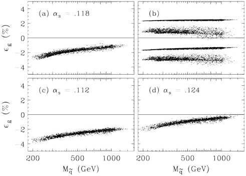
Figure 2: (a), (c), (d) Threshold corrections at the grand unification scale, $\epsilon_{g}=(1-g_{1}/g_{3})(M_{GUT})$, necessary to achieve a value of the low energy strong gauge coupling, as a function of $M_{\tilde{q}}$ for a generic supergravity spectrum. (b) The maximum and minimum $\epsilon_{g}$ allowed in minimal SU(5) (two top regions) and missing doublet SU(5) (bottom two regions).

Apart from the possibilities of having a $T_{SUSY}\simeq 1$ TeV, or a complicated structure of GUT threshold corrections GUTthr , one may also consider the existence of non-renormalizable operators of the kind $\Sigma F_{\mu\nu}F^{\mu\nu}/M_{Pl}$, which in minimal models, with one adjoint $\Sigma$, are unique at leading order in powers of $1/M_{Pl}$. Tevatron searches have the potential of testing squark and gaugino masses consistent with the low energy values shown in Figure 2.

Finally, let us consider an interesting property of the renormalization group evolution of the gauge couplings pointed out by Shifman Shifman . In the $\overline{DR}$ scheme, the two-loop contribution of a supermultiplet to the renormalization group evolution of the gauge couplings from the scale $M_{G}$ up to the scale $Q>M_{\eta}$ can be given by

$$\Delta^{\eta}\alpha_{i}^{-1}(Q)=\frac{b_{i}^{\eta}}{2\pi}\ln\left(\frac{M_{G}}{QZ_{\eta}}\right),$$ (29)

where $Z_{\eta}$ is the one-loop wave function renormalization constant associated with the supermultiplet $\eta$. Observe that this is a compact expression that parametrizes the two-loop contributions to the evolution of the gauge couplings, by knowledge of $Z_{\eta}$ at the one-loop order. Now, assume a vector like supermultiplet $\eta$+$\overline{\eta}$, which acquires an explicit supersymmetry conserving mass $M_{\eta}^{G}$ at the GUT scale (via an explicit term in the superpotential). Its renormalized mass will be given by $M_{\eta}^{G}/Z_{\eta}$. Hence, after decoupling of this particle at the scale $M_{\eta}>M_{Z}$,

$$\Delta^{\eta+\bar{\eta}}\alpha_{i}^{-1}(M_{Z})=\frac{b_{i}^{\eta}}{\pi}ln\left(\frac{M_{G}}{M_{\eta}^{G}}\right).$$ (30)

Observe that the above formula does not mean that vector like multiplets do not affect the evolution of the gauge couplings beyond the one-loop order, since their presence affects the value of the wave function renormalization constant of all the other particles present in the spectrum Ross . Indeed, the overall effect of vector like particles belonging to complete representations of $SU(5)$, whose effect in the prediction of $\alpha_{3}(M_{Z})$ vanishes at one-loop order, is to enhance the two-loop effects on the unification relations, leading to a value of $\alpha_{3}(M_{Z})$ larger than in the MSSM.

II.1 Yukawa Coupling Unification

The unification of the bottom and $\tau$ Yukawa couplings at the grand unification scale is a property of the simplest unfication scenarios. For the present experimental allowed range of values for the top quark mass PDB , $M_{t}=173.8\pm 5.2$ GeV, and the strong gauge coupling, the condition of bottom-tau Yukawa coupling unification implies either low values of $\tan\beta$, $1.5\stackrel{{\scriptstyle<}}{{{}_{\sim}}}\tan\beta\stackrel{{\scriptstyle<}}{{{}_{\sim}}}3$, or very large values of $\tan\beta\stackrel{{\scriptstyle>}}{{{}_{\sim}}}20$ Ramond –largetb . Most interesting is the fact that to achieve b-$\tau$ unification, $h_{b}(M_{GUT})=h_{\tau}(M_{GUT})$, large values of the top Yukawa coupling, $h_{t}$, at $M_{GUT}$ are necessary in order to compensate for the effects of the strong interaction renormalization in the running of the bottom Yukawa coupling. These large values of $h_{t}^{2}(M_{GUT})/4\pi\simeq$ 0.1–1 are exactly those that ensure the attraction towards the infrared (IR) fixed point solution of the top quark mass CPW ; Yukawa ; LP1 . The exact value of the running bottom mass $m_{b}(M_{b})\simeq$ 4.15–4.35 GeV, is very important to determine the top quark mass predictions BCPW ; KKRW . A larger $m_{b}$, for instance, will be associated with a larger bottom Yukawa coupling at low energies, allowing unification for smaller values of the top Yukawa coupling, an effect that can be enhanced by relaxing the exact unification conditions KKRW ; EPS ; NIRlast .

For $M_{GUT}\simeq 2\times 10^{16}$ GeV, the infrared fixed point value of the top Yukawa coupling $(h_{t}^{IR})^{2}/4\pi\simeq(8/9)\alpha_{s}(M_{Z})$, and the corresponding running top quark mass $m_{t}^{IR}\simeq h_{t}^{IR}v\sin\beta$, with $v\simeq 174$ GeV. After the computation of the proper low energy threshold corrections NIRlast ; NIRref , the infrared fixed point solution associates to each value of $M_{t}$ the lowest possible value of $\tan\beta$ consistent with the validity of perturbation theory up to scales of order $M_{GUT}$. The most interesting consequence of the IR fixed point $M_{t}$–$\tan\beta$ relation is associated with the lightest CP-even Higgs mass predictions in the MSSM COPW ; BABE . Indeed, for $\tan\beta$ larger than 1, the lowest tree level value of the lightest Higgs mass, $m_{h}$, is obtained at the lowest value of $\tan\beta$, a property that holds even after including two-loop corrections. For squark masses below or of the order of 1 TeV, the present experimental bounds on the Higgs mass begin to constraint in a relevant way the low $\tan\beta$ solution to bottom-tau Yukawa coupling unification CEH ; CCPW .

In the context of $b$–$\tau$ Yukawa coupling unification possible large radiative corrections to the bottom mass are crucial in determining the top quark mass and $\tan\beta$ predictions. In general, one assumes that the top and bottom quarks couple each to only one of the Higgs doublets and hence $m_{t}(M_{t})=h_{t}(M_{t})v_{2}$ and $m_{b}(M_{t})=h_{b}(M_{t})v_{1}$, with $v_{i}$ the vacuum expectation value of the Higgs $H_{i}$. However, a coupling of the bottom (top) quark to the neutral component of the Higgs $H_{2(1)}$ may be generated at the one-loop level, and since $v_{2}\gg v_{1}$ for large values of $\tan\beta>10$, large corrections to the bottom mass may be present Hall ; wefour ; CDWR ; Steve ,

$$m_{b} = h_{b}\;v_{1}+\Delta h_{b}\;v_{2}\equiv h_{b}v_{1}(1+K\tan\beta).$$ (31)

$\Delta m_{b}=K\tan\beta$ receives contributions from stop-chargino and sbottom-gluino loops, the latter being the dominant ones. The magnitude of $\Delta m_{b}$ is strongly dependent on the supersymmetric spectrum and its sign is generally governed by the overall sign of $\mu\times m_{\tilde{g}}$,

$$K = \mu\;m_{\tilde{g}}\;\tan\beta\;\;\left[\frac{2\alpha_{s}}{3\pi}I_{1}(m^{2}_{\tilde{b}_{1}},m^{2}_{\tilde{b}_{2}},m^{2}_{\tilde{g}})+\frac{A_{t}}{m_{\tilde{g}}}\frac{h_{t}^{2}}{(4\pi)^{2}}I_{2}(m^{2}_{\tilde{t}_{1}},m^{2}_{\tilde{t}_{2}},\mu^{2})\right],$$ (32)

where $m_{\tilde{b}_{i}}$ and $m_{\tilde{t}_{i}}$ are the sbottom and stop mass eigenstates, respectively, the integral factor is $I_{i}=C_{i}/a_{max}$, with $a_{max}$ the maximum of the squared masses, and $C_{i}$ = 0.5–0.9 depending on the mass splitting. Using the relation $m_{\tilde{g}}\simeq$ 2.6–2.8 $M_{1/2}$ and the fact that from the renormalization group equations, $A_{t}$ is in general of opposite sign to $M_{1/2}$ and of ${\cal{O}}(M_{1/2})$, it follows that there is a partial cancellation between the two terms in Eq. (32). Although important, such partial cancellation is in general not sufficient to render the bottom mass corrections small. Hence, in the large $\tan\beta$ region, the bottom mass corrections need to be appropriately computed to extract the proper value of the bottom Yukawa coupling at low energies. The predictions from $b$–$\tau$ Yukawa coupling unification will therefore depend on the particular supersymmetric spectrum under consideration. In particular, the exact value of $\tan\beta$ at which the unification of Yukawa couplings is achieved depends strongly on the size of the $\Delta m_{b}$ corrections CDWR ; MP ; CEP . In Figure 3 the effect of the bottom mass corrections is displayed. A value of the running bottom mass $m_{b}(M_{b})=4.15$ GeV has been used. For values of the strong gauge coupling $\alpha_{3}(M_{Z})\stackrel{{\scriptstyle>}}{{{}_{\sim}}}0.12$ unification in the low $\tan\beta$ regime demands slightly larger values of the running bottom mass, $m_{b}(M_{b})\stackrel{{\scriptstyle>}}{{{}_{\sim}}}4.25$ GeV.

Figure 3: Top quark mass predictions coming from the condition of bottom-tau Yukawa unification, for different values of the bottom mass corrections, parametrized by $\Delta m_{b}=-K_{c}\tan\beta$, for $K_{c}=0$ (dashed-line), 0.003 (dotted line) and 0.006 (dot-dashed ine). The solid line represent the ratio $\omega$ of the bottom-Yukawa coupling to the top-Yukawa coupling at the GUT scale, $\omega=$ 1, 0.6 and 0.2, respectively. The curves are cut when the value of $h_{t}^{2}(M_{GUT})/4\pi\geq 1$.

The sign of the bottom mass corrections is also related to the one of the supersymmetric contributions to the amplitude of the $b\rightarrow s\gamma$ decay process in models with universal soft supersymmetry breaking parameters at high energies. In these models, the most important supersymmetric contribution to the $b\rightarrow s\gamma$ decay rate comes from the chargino-stop one-loop diagram bsga . The chargino contribution to the $b\rightarrow s\gamma$ decay amplitude depends on the soft supersymmetry breaking mass parameter $A_{t}$ and on the supersymmetric mass parameter $\mu$, and for very large values of $\tan\beta$, it is given by Diaz ; BOP ,

$$A_{\tilde{\chi}^{+}}\simeq\frac{m_{t}^{2}}{m_{\tilde{t}}^{2}}\frac{A_{t}\mu}{m_{\tilde{t}}^{2}}\tan\beta\;G\left(\frac{m_{\tilde{t}}^{2}}{\mu^{2}}\right),$$ (33)

where $G(x)$ is a function that takes values of order 1 when the characteristic stop mass $m_{\tilde{t}}$ is of order $\mu$ and grows for lower values of $\mu$. One can show that, for positive (negative) values of $A_{t}\times\mu$ the chargino contributions are of the same (opposite) sign as the charged Higgs ones wefour . Hence, to partially cancel the light charged Higgs contributions, rendering the $b\rightarrow s\gamma$ decay rate acceptable, negative values for $A_{t}\times\mu$ are required. As follows from Eq. (32) and the discussion below, this requirement has direct implications on the corrections to the bottom mass and, after a detailed analysis, one concludes that it puts strong constraints on models with Yukawa coupling unification wefour ; BOP . It is important to remark, however, that these constraints can be evaded if small flavor violating up or down squark mixing effects are present in the low energy spectrum CEP ; Steve ; Masiero .

Finally, it is important to remark that, in the context of SO(10) unification scenarios which predict the unification of the top and the neutrino Yukawa couplings at the scale $M_{G}$, the unification predictions depend strongly on the mass of the right handed neutrinos. In particular, a value of the right handed $\tau$ neutrino mass smaller than $10^{15}$ GeV would put very strong constraints on bottom-$\tau$ Yukawa coupling unification in the small $\tan\beta$ regime neutrinos .

III The Minimal Supersymmetric Model

III.1 The Lagrangian Density

The minimal supersymmetric standard model (MSSM) is the minimal supersymmetric extension of the standard model (SM) with

1. two Higgs doublets $H_{1}$ and $H_{2}$ such that $H_{1}$ couples to the fermions with $t_{3}=-1/2$ and $H_{2}$ couples to the fermions with $t_{3}=+1/2$,

2. a supersymmetric partner for each SM particle and every Higgs boson,

3. a conserved $R$-parity $R\equiv(-1)^{3B+L+2S}=(-1)^{3(B-L)+2S}$,

4. a Higgs mixing parameter $\mu$ assumed to be real,

5. three real symmetric $3\times 3$ matrices of squark mass-squared parameters, $M_{\widetilde{Q}}^{2}$, $M_{\widetilde{U}}^{2}$ and $M_{\widetilde{D}}^{2}$,

6. two real symmetric $3\times 3$ matrices of slepton mass-squared parameters, $M_{\widetilde{L}}^{2}$ and $M_{\widetilde{E}}^{2}$, and

7. three real $3\times 3$ matrices of trilinear Yukawa parameters, $A_{U}$, $A_{D}$ and $A_{E}$.

The fields in the MSSM are summarized in a table as the following:

Superfield	Bosonic Fields	Fermionic Fields
$\widehat{G}$	Gluons: $g^{a},a=1,...,8$	Gluinos: $\tilde{g}^{a}$
$\widehat{W}$	$W$ Bosons: $W^{\alpha},\alpha=1,2,3$	Winos: $\widetilde{W}^{\alpha}$
$\widehat{B}$	$B$ Boson: $B$	Bino: $\widetilde{B}$
$\widehat{Q}$	Squarks: $\widetilde{Q}=(\tilde{u}_{L},\tilde{d}_{L})$	Quarks: $Q=(u_{L},d_{L})$
$\widehat{U}$	Squarks: $\widetilde{U}=\tilde{u}_{R}^{*}$	Quarks: $U=u_{L}^{c}$
$\widehat{D}$	Squarks: $\widetilde{D}=\tilde{d}_{R}^{*}$	Quarks: $D=d_{L}^{c}$
$\widehat{L}$	Sleptons: $\widetilde{L}=(\tilde{\nu}_{L},\tilde{\ell}_{L})$	Leptons: $L=(\nu_{L},\ell_{L})$
$\widehat{E}$	Sleptons: $\widetilde{E}=\tilde{\ell}_{R}^{*}$	Leptons: $E=\ell_{L}^{c}$
$\widehat{H}_{1}$	Higgs bosons: $H_{1}=(H_{1}^{0},H_{1}^{-})$	Higgsinos: $\widetilde{H}_{1}=(\widetilde{H}_{1}^{0},\widetilde{H}_{1}^{-})$
$\widehat{H}_{2}$	Higgs bosons: $H_{2}=(H_{2}^{+},H_{2}^{0})$	Higgsinos: $\widetilde{H}_{2}=(\widetilde{H}_{2}^{+},\widetilde{H}_{2}^{0})$

where $U,u=u,\;c$ and $t$; $D,d=d,\;s$ and $b$; and $E,\ell=e,\mu$ and $\tau$. In this model, the lightest supersymmetric particle (LSP) is stable.

The MSSM Langrangian density with soft supersymmetry breaking terms has the following form

$${\cal L}_{\rm soft} = -m_{H_{1}}^{2}|H_{1}|^{2}-m_{H_{2}}^{2}|H_{2}|^{2}+\mu B\epsilon_{ij}\left(H_{1}^{i}H_{2}^{j}+H.c.\right)$$ (34)

$$-{1\over 2}M_{1}\overline{\widetilde{B}}{B}-{1\over 2}M_{2}\overline{\widetilde{W}^{\alpha}}\widetilde{W}^{\alpha}-{1\over 2}M_{3}\overline{\tilde{g}^{a}}\tilde{g}^{a}$$

$$-M_{\widetilde{Q}}^{2}[\tilde{u}_{L}^{*}\tilde{u}_{L}+\tilde{d}_{L}^{*}\tilde{d}_{L}]-M_{\widetilde{U}}^{2}\tilde{u}_{R}^{*}\tilde{u}_{R}-M_{\widetilde{D}}^{2}\tilde{d}_{R}^{*}\tilde{d}_{R}$$

$$-M_{\widetilde{L}}^{2}[\tilde{\ell}_{L}^{*}\tilde{\ell}_{L}+\tilde{\nu}_{L}^{*}\tilde{\nu}_{L}]-M_{\widetilde{E}}^{2}\tilde{\ell}_{R}^{*}\tilde{\ell}_{R}$$

$$-\epsilon_{ij}\left(-\lambda_{u}A_{U}H_{2}^{i}\widetilde{Q}^{j}\tilde{u}_{R}^{*}+\lambda_{d}A_{D}H_{1}^{i}\widetilde{Q}^{j}\tilde{d}_{R}^{*}+\lambda_{\ell}A_{E}H_{1}^{i}\widetilde{L}^{j}\tilde{\ell}_{R}^{*}\right)\;,$$

where

$$Q = \left(\begin{array}[]{c}u_{L}\\ d_{L}\end{array}\right),\;\;L=\left(\begin{array}[]{c}\nu_{L}\\ \ell_{L}\end{array}\right),\;\;H_{1}=\left(\begin{array}[]{c}H_{1}^{0}\\ H_{1}^{-}\end{array}\right),\;\;{\rm and}\;\;H_{2}=\left(\begin{array}[]{c}H_{2}^{+}\\ H_{2}^{0}\end{array}\right),$$ (43)

$$\widetilde{Q} = \left(\begin{array}[]{c}\tilde{u}_{L}\\ \tilde{d}_{L}\end{array}\right),\;\;\widetilde{L}=\left(\begin{array}[]{c}\tilde{\nu}_{L}\\ \tilde{\ell}_{L}\end{array}\right),\;\;\widetilde{H}_{1}=\left(\begin{array}[]{c}\widetilde{H}_{1}^{0}\\ \widetilde{H}_{1}^{-}\end{array}\right),\;\;{\rm and}\;\;\widetilde{H}_{2}=\left(\begin{array}[]{c}\widetilde{H}_{2}^{+}\\ \widetilde{H}_{2}^{0}\end{array}\right)\;,$$ (52)

$U,u=u,\;c$ and $t$; $D,d=d,\;s$ and $b$; $E,\ell=e,\;\mu$ and $\tau$; and $\epsilon_{ij}$ is the antisymmetric tensor with $i,j=1,\;2$ and $\epsilon_{12}=1$. The tree-level Yukawa couplings are defined by

$$\lambda_{u}={{\sqrt{2}m_{u}}\over{v\sin\beta}}\;,\qquad\lambda_{d}={{\sqrt{2}m_{d}}\over{v\cos\beta}}\;,\qquad\lambda_{\ell}={{\sqrt{2}m_{\ell}}\over{v\cos\beta}}\;,$$ (53)

where $\tan\beta=v_{2}/v_{1}$ is the ratio of the vacuum expectation values of $H_{2}^{0}$ and $H_{1}^{0}$. The $\mu$ term in the superpotential contributes to the Higgs potential which at tree level is

$$V_{\rm Higgs} = (m_{H_{1}}^{2}+\mu^{2})|H_{1}|^{2}+(m_{H_{2}}^{2}+\mu^{2})|H_{2}|^{2}-m_{3}^{2}(\epsilon_{ij}{H_{1}}^{i}{H_{2}}^{j}+{\rm H.c.})$$ (54)

$$+{1\over 8}(g^{2}+g^{\prime 2})\left[|H_{1}|^{2}-|H_{2}|^{2}\right]^{2}+{1\over 2}g^{2}|H_{1}^{i*}H_{2}^{i}|^{2}\;,$$

where $m_{H_{1}}$, $m_{H_{2}}$, and $m_{3}$ are soft-supersymmetry breaking parameters. We shall define as usual the soft Higgs mass parameters

$$m_{1}^{2} = m_{H_{1}}^{2}+\mu^{2}\;,$$

$$m_{2}^{2} = m_{H_{2}}^{2}+\mu^{2}\;,$$

$$m_{3}^{2} = B\mu\;.$$ (55)

Of the eight degrees of freedom in the two Higgs doublets, three Goldstone bosons ($G^{\pm}$, $G^{0}$) are absorbed to give the $W^{\pm}$ and the $Z$ masses, leaving five physical Higgs bosons: the charged Higgs bosons $H^{\pm}$, the CP-even Higgs bosons $h^{0}$ (lighter) and $H^{0}$ (heavier), and the CP-odd Higgs boson $A^{0}$.

III.2 The Mass Matrices

In this section, the mass matrices of gauginos, top squarks, bottom squarks and the tau sleptons are presented in the gauge eigenstates. The chargino mass matrix in the ($\widetilde{W}^{+},\widetilde{H}^{+}$) basis is

$${\cal M}_{C}=\left(\begin{array}[]{c@{\quad}c}M_{2}&\sqrt{2}M_{W}\sin\beta\\ \sqrt{2}M_{W}\cos\beta&+\mu\end{array}\right)\;.$$ (56)

This mass matrix is not symmetric and must be diagonalized by two matrices Haber .

The neutralino mass matrix in the basis of ($\widetilde{B},\widetilde{W}^{3},\widetilde{H}^{0}_{1},\widetilde{H}^{0}_{2}$) is

$${\cal M}_{N}=\left(\begin{array}[]{cccc}M_{1}&0&-M_{Z}\cos\beta\sin\theta_{W}&M_{Z}\sin\beta\sin\theta_{W}\\ 0&M_{2}&M_{Z}\cos\beta\cos\theta_{W}&-M_{Z}\sin\beta\cos\theta_{W}\\ -M_{Z}\cos\beta\sin\theta_{W}&M_{Z}\cos\beta\cos\theta_{W}&0&-\mu\\ M_{Z}\sin\beta\sin\theta_{W}&-M_{Z}\sin\beta\cos\theta_{W}&-\mu&0\end{array}\right)\;.$$ (57)

This mass matrix is symmetric and can be diagonalized by a single matrix Haber .

The top squark, bottom squark and the tau slepton mass-squared matrices in the ($\tilde{f}_{L},\tilde{f}_{R}$) basis are expressed as

$${\cal M}_{\tilde{t}}^{2}=\left(\begin{array}[]{c@{\quad}c}m_{\widetilde{Q}}^{2}+m_{t}^{2}+{1\over 6}(4M_{W}^{2}-M_{Z}^{2})\cos 2\beta&m_{t}(A_{t}-\mu\cot\beta)\\ m_{t}(A_{t}-\mu\cot\beta)&m_{\tilde{t}_{R}}^{2}+m_{t}^{2}-{2\over 3}(M_{W}^{2}-M_{Z}^{2})\cos 2\beta\end{array}\right)\;,$$ (58)

$${\cal M}_{\tilde{b}}^{2}=\left(\begin{array}[]{c@{\quad}c}m_{\widetilde{Q}}^{2}+m_{b}^{2}-{1\over 6}(2M_{W}^{2}+M_{Z}^{2})\cos 2\beta&m_{b}(A_{b}-\mu\tan\beta)\\ m_{b}(A_{b}-\mu\tan\beta)&m_{\tilde{b}_{R}}^{2}+m_{b}^{2}+{1\over 3}(M_{W}^{2}-M_{Z}^{2})\cos 2\beta\end{array}\right)\;,$$ (59)

$${\cal M}_{\tilde{\tau}}^{2}=\left(\begin{array}[]{c@{\quad}c}m_{\widetilde{L}}^{2}+m_{\tau}^{2}-{1\over 2}(2M_{W}^{2}-M_{Z}^{2})\cos 2\beta&m_{\tau}(A_{\tau}-\mu\tan\beta)\\ m_{\tau}(A_{\tau}-\mu\tan\beta)&m_{\tilde{\tau}_{R}}^{2}+m_{\tau}^{2}+(M_{W}^{2}-M_{Z}^{2})\cos 2\beta\end{array}\right)\;,$$ (60)

which are diagonalized by orthogonal matrices with mixing angles $\theta_{\tilde{t}}$, $\theta_{\tilde{b}}$, and $\theta_{\tilde{\tau}}$. The mass eigenstate for the massive third generation sneutrino is

$$M_{\tilde{\nu}}^{2} = M_{\widetilde{L}}^{2}+{1\over 2}{M_{Z}^{2}}\cos 2\beta\;.$$ (61)

In the mass eigenstates, we label the charginos, the neutralinos and the sfermions such that

• $m_{\tilde{\chi}_{1}^{\pm}}<m_{\tilde{\chi}_{2}^{\pm}}$,

• $m_{\tilde{\chi}_{1}^{0}}<m_{\tilde{\chi}_{2}^{0}}<M_{\tilde{\chi}_{3}^{0}}<m_{\tilde{\chi}_{4}^{0}}$, and

• $m_{\tilde{t}_{1}}<m_{\tilde{t}_{2}}$, $m_{\tilde{b}_{1}}<m_{\tilde{b}_{2}}$, and $m_{\tilde{\tau}_{1}}<m_{\tilde{\tau}_{2}}$.

III.3 Mass Eigenstates of Top Squarks

The mass eigenstates of the top squarks are defined as

$$\left(\begin{array}[]{c}\tilde{t}_{1}\\ \tilde{t}_{2}\end{array}\right) \equiv \left(\begin{array}[]{rr}\cos\theta_{\tilde{t}}&\sin\theta_{\tilde{t}}\\ -\sin\theta_{\tilde{t}}&\cos\theta_{\tilde{t}}\end{array}\right)\left(\begin{array}[]{c}\tilde{t}_{L}\\ \tilde{t}_{R}\end{array}\right),$$ (68)

$$\tilde{t}_{L} = \cos\theta_{\tilde{t}}\tilde{t}_{1}-\sin\theta_{\tilde{t}}\tilde{t}_{2},$$

$$\tilde{t}_{R} = \sin\theta_{\tilde{t}}\tilde{t}_{1}+\cos\theta_{\tilde{t}}\tilde{t}_{2}$$ (69)

The mass matrix in the basis of ($\tilde{t}_{L},\tilde{t}_{R}$) and its eigenvalues are

$${\cal M}_{\tilde{t}}^{2} \equiv \left(\begin{array}[]{ll}m_{LL}&m_{LR}\\ m_{LR}&m_{RR}\end{array}\right),$$ (72)

$$m_{\pm}^{2} = \frac{1}{2}[(m_{LL}+m_{RR})\pm\Delta],$$

$$\Delta = [(m_{LL}-m_{RR})^{2}+4m_{LR}^{2}]^{1/2}$$ (73)

where

$$m_{LL} = m_{\tilde{Q}_{L}}^{2}+m_{t}^{2}+M_{Z}^{2}\cos 2\beta(+C_{L}),$$

$$m_{RR} = m_{\tilde{t}_{R}}^{2}+m_{t}^{2}+M_{Z}^{2}\cos 2\beta(-C_{R}),$$

$$m_{LR} = m_{t}(A_{t}-\mu\cot\beta),$$ (74)

$C_{L}=1/2-\frac{2}{3}\sin^{2}\theta_{W}$ and $C_{R}=-\frac{2}{3}\sin^{2}\theta_{W}$.

Requiring $m_{\tilde{t}_{1}}<m_{\tilde{t}_{2}}$, we have

$$m_{\tilde{t}_{1}}^{2} = m_{-}^{2}=m_{t}^{2}+\frac{1}{2}(m_{\tilde{Q}_{L}}^{2}+m_{\tilde{t}_{R}}^{2})+\frac{1}{4}(M_{Z}^{2}\cos 2\beta)-\frac{\Delta}{2},$$

$$m_{\tilde{t}_{2}}^{2} = m_{+}^{2}=m_{t}^{2}+\frac{1}{2}(m_{\tilde{Q}_{L}}^{2}+m_{\tilde{t}_{R}}^{2})+\frac{1}{4}(M_{Z}^{2}\cos 2\beta)+\frac{\Delta}{2},$$ (75)

$$\Delta = \{[(m_{\tilde{Q}_{L}}^{2}-m_{\tilde{t}_{R}}^{2})+\frac{\cos 2\beta}{6}(8M_{W}^{2}-5M_{Z}^{2})]^{2}+4m_{t}^{2}(A_{t}-\mu\cot\beta)^{2}\}^{1/2}$$

The mixing angle $\theta_{\tilde{t}}$ can be evaluated from $\tan\theta_{\tilde{t}}$,

$$\tan\theta_{\tilde{t}}=\frac{m_{\tilde{t}_{1}}^{2}-m_{LL}}{m_{LR}}.$$ (76)

The conventions for the top squark mass eigenstates and the mixing angle can be generalized to other scalar fermions.

III.4 Bridging Various Conventions

In this section, we list various conventions previously used by members in the mSUGRA working group. To obtain the same SUSY mass spectrum with the conventions in this report, the following modifications can be applied for $\mu$ and $A_{t}$,

Collaboration	$\mu$	$A_{t}$
ISAJET	the same	the same
SPYTHIA	the same	the same
Arnowitt and Nath	the same	$A_{t}\to-A_{t}$
Baer and Tata	the same	the same
Barger, Berger and Ohmann	$\mu\to-\mu$	the same
Carena and Wagner	the same	the same
Chankowski and Pokorski	the same	the same
Drees and Nojiri	the same	$A_{t}\to-A_{t}$
Ellis et al.	the same	$A_{t}\to-A_{t}$
Haber and Kane	the same	the same
Langacker and Polonsky	$\mu\to-\mu$	the same
Nilles	$\mu\to-\mu$	the same
Martin and Ramond	the same	$A_{t}\to-A_{t}$
Pierce et al.	$\mu\to-\mu$	the same
Kunszt and Zwirner	$\mu\to-\mu$	the same

IV Renormalization Group Equation Evolution and SUSY Particle Mass Spectra

IV.1 Renormalization Group Equations

The mSUGRA model is characterized by relatively few parameters (five) at a high energy near the Planck scale. To translate these parameters into masses and mixings for the supersymmetric particles that might be observed in an experiment, one must apply the Renormalization Group (RG) equations to the parameters of the model. The five parameters are treated as boundary conditions for the coupled set of RG equations, and the resulting gauge, Yukawa, and soft supersymmetry breaking parameters defined with the running scale near the electroweak scale enter into the MSSM Lagrangian, providing predictions and correlations between the various particles in the SUSY spectrum. Some recent analyses of the mass patterns in the mSUGRA model can be found in Refs. masses ; bbo2 .

The renormalization equations for the gauge couplings and the Yukawa couplings to one-loop order are (with $t=\ln(Q/Q_{0})$)

$${{dg_{i}}\over{dt}}={b_{i}g_{i}^{3}\over{16\pi^{2}}}\;,$$ (77)

$${{d{\bf U}}\over{dt}} = {1\over{16\pi^{2}}}\Big{[}-\sum c_{i}g_{i}^{2}+3{\bf UU^{\dagger}}+{\bf DD^{\dagger}}+{\bf Tr}[3{\bf UU^{\dagger}}]\Big{]}{\bf U}\;,$$ (78)

$${{d{\bf D}}\over{dt}} = {1\over{16\pi^{2}}}\Big{[}-\sum c_{i}^{\prime}g_{i}^{2}+3{\bf DD^{\dagger}}+{\bf UU^{\dagger}}+{\bf Tr}[3{\bf DD^{\dagger}}+{\bf EE^{\dagger}}]\Big{]}{\bf D}\;,$$ (79)

$${{d{\bf E}}\over{dt}} = {1\over{16\pi^{2}}}\Big{[}-\sum c_{i}^{\prime\prime}g_{i}^{2}+3{\bf EE^{\dagger}}+{\bf Tr}[3{\bf DD^{\dagger}}+{\bf EE^{\dagger}}]\Big{]}{\bf E}\;,$$ (80)

where

$$b_{i}=({33\over 5},1,-3)\;,\qquad c_{i}=({13\over 15},3,{16\over 3})\;,\qquad c_{i}^{\prime}=({7\over 15},3,{16\over 3})\;,\qquad c_{i}^{\prime\prime}=({9\over 5},3,0)\;.$$ (81)

In the most general case shown above, the evolution equations involve matrices. For example the Yukawa couplings form three-by-three Yukawa matrices: ${\bf U}$ for the up-type quarks, ${\bf D}$ for the down-type quarks, and ${\bf E}$ for the charged leptons. Similarly the soft-supersymmetry breaking parameters form the matrices ${\bf M}^{2}_{Q_{L}}$, ${\bf M}^{2}_{U_{R}}$, ${\bf M}^{2}_{D_{R}}$, ${\bf M}^{2}_{L_{L}}$, and ${\bf M}^{2}_{E_{R}}$ giving masses to the scalar supersymmetric particles. Finally there are in general matrices for the trilinear soft-supersymmetry breaking “A-terms”: ${\bf A_{U}}$, ${\bf A_{D}}$, and ${\bf A_{E}}$. Since soft SUSY breaking trilinear scalar interactions are given by corresponding terms in the superpotential (with superfields set to scalar components) times an $A$-parameter, it turns out to be useful to define the combinations ${\bf U_{A}}_{ij}\equiv{\bf A_{U}}_{ij}{\bf U}_{ij}$, etc. in the matrix version of the RG equations. Then the evolution of the soft-supersymmetry parameters (with our convention for signs) is given by the following renormalization group equationsbbo2 ; bbmr

$${{dM_{i}}\over{dt}} = {2\over{16\pi^{2}}}b_{i}g_{i}^{2}M_{i}\;,$$ (82)

$${{d{\bf U_{A}}}\over{dt}} = {1\over{16\pi^{2}}}\Bigg{[}-\Big{(}{13\over 15}g_{1}^{2}+3g_{2}^{2}+{16\over 3}g_{3}^{2}\Big{)}{\bf U_{A}}+2\Big{(}{13\over 15}g_{1}^{2}{M_{1}}+3g_{2}^{2}{M_{2}}+{16\over 3}g_{3}^{2}{M_{3}}\Big{)}{\bf U}$$ (83)

$$+\Big{\{}\Big{[}4({\bf U_{A}U^{\dagger}U})+6{\bf Tr}({\bf U_{A}U^{\dagger}}){\bf U}\Big{]}+\Big{[}5({\bf UU^{\dagger}U_{A}})+3{\bf Tr}({\bf UU^{\dagger}}){\bf U_{A}}\Big{]}$$

$$+2({\bf D_{A}D^{\dagger}U})+({\bf DD^{\dagger}U_{A}})\Big{\}}\Bigg{]}\;,$$

$${{d{\bf D_{A}}}\over{dt}} = {1\over{16\pi^{2}}}\Bigg{[}-\Big{(}{7\over 15}g_{1}^{2}+3g_{2}^{2}+{16\over 3}g_{3}^{2}\Big{)}{\bf D_{A}}+2\Big{(}{7\over 15}g_{1}^{2}{M_{1}}+3g_{2}^{2}{M_{2}}+{16\over 3}g_{3}^{2}{M_{3}}\Big{)}{\bf D}$$ (84)

$$+\Big{\{}\Big{[}4({\bf D_{A}D^{\dagger}D})+6{\bf Tr}({\bf D_{A}D^{\dagger}}){\bf D}\Big{]}+\Big{[}5({\bf DD^{\dagger}D_{A}})+3{\bf Tr}({\bf DD^{\dagger}}){\bf D_{A}}\Big{]}$$

$$+2({\bf U_{A}U^{\dagger}D})+({\bf UU^{\dagger}D_{A}})+2{\bf Tr}({\bf E_{A}E^{\dagger}}){\bf D}+{\bf Tr}({\bf EE^{\dagger}}){\bf D_{A}}\Big{\}}\Bigg{]}\;,$$

$${{d{\bf E_{A}}}\over{dt}} = {1\over{16\pi^{2}}}\Bigg{[}-\Big{(}3g_{1}^{2}+3g_{2}^{2}\Big{)}{\bf E_{A}}+2\Big{(}3g_{1}^{2}{M_{1}}+3g_{2}^{2}{M_{2}}\Big{)}{\bf E}$$ (85)

$$+\Big{\{}\Big{[}4({\bf E_{A}E^{\dagger}E})+2{\bf Tr}({\bf E_{A}E^{\dagger}}){\bf E}\Big{]}+\Big{[}5({\bf EE^{\dagger}E_{A}})+{\bf Tr}({\bf EE^{\dagger}}){\bf E_{A}}\Big{]}$$

$$+6({\bf D_{A}D^{\dagger}E})+3({\bf DD^{\dagger}E_{A}})\Big{\}}\Bigg{]}\;,$$

$${{dB}\over{dt}} = {2\over{16\pi^{2}}}\Big{(}{3\over 5}g_{1}^{2}M_{1}+3g_{2}^{2}M_{2}+{\bf Tr}(3{\bf UU_{A}}+3{\bf DD_{A}}+{\bf EE_{A}})\Big{)}\;,$$ (86)

$${{d\mu}\over{dt}} = {\mu\over{16\pi^{2}}}\Big{(}-{3\over 5}g_{1}^{2}-3g_{2}^{2}+{\bf Tr}(3{\bf UU^{\dagger}}+3{\bf DD^{\dagger}}+{\bf EE^{\dagger}})\Big{)}\;,$$ (87)

$${{dm_{H_{1}}^{2}}\over{dt}} = {2\over{16\pi^{2}}}\Big{(}-{3\over 5}g_{1}^{2}M_{1}^{2}-3g_{2}^{2}M_{2}^{2}$$ (88)

$$+3{\bf Tr}({\bf D}({\bf M}_{Q_{L}}^{2}+{\bf M}_{D_{R}}^{2}){\bf D^{\dagger}}+m_{H_{1}}^{2}{\bf DD^{\dagger}}+{\bf D_{A}D_{A}^{\dagger}})$$

$$+{\bf Tr}({\bf E}({\bf M}_{L_{L}}^{2}+{\bf M}_{E_{R}}^{2}){\bf E^{\dagger}}+m_{H_{1}}^{2}{\bf EE^{\dagger}}+{\bf E_{A}E_{A}^{\dagger}})\Big{)}\;,$$

$${{dm_{H_{2}}^{2}}\over{dt}} = {2\over{16\pi^{2}}}\Big{(}-{3\over 5}g_{1}^{2}M_{1}^{2}-3g_{2}^{2}M_{2}^{2}$$ (89)

$$+3{\bf Tr}({\bf U}({\bf M}_{Q_{L}}^{2}+{\bf M}_{U_{R}}^{2}){\bf U^{\dagger}}+m_{H_{2}}^{2}{\bf UU^{\dagger}}+{\bf U_{A}U_{A}^{\dagger}})\Big{)}\;,$$

$${{d{\bf M}_{Q_{L}}^{2}}\over{dt}} = {2\over{16\pi^{2}}}\Big{(}-{1\over 15}g_{1}^{2}M_{1}^{2}-3g_{2}^{2}M_{2}^{2}-{16\over 3}g_{3}^{2}M_{3}^{2}$$ (90)

$$+{1\over 2}[{\bf UU^{\dagger}}{\bf M}_{Q_{L}}^{2}+{\bf M}_{Q_{L}}^{2}{\bf UU^{\dagger}}+2({\bf U}{\bf M}_{U_{R}}^{2}{\bf U^{\dagger}}+m_{H_{2}}^{2}{\bf UU^{\dagger}}+{\bf U_{A}U_{A}^{\dagger}})]$$

$$+{1\over 2}[{\bf DD^{\dagger}}{\bf M}_{Q_{L}}^{2}+{\bf M}_{Q_{L}}^{2}{\bf DD^{\dagger}}+2({\bf D}{\bf M}_{D_{R}}^{2}{\bf D^{\dagger}}+m_{H_{1}}^{2}{\bf DD^{\dagger}}+{\bf D_{A}D_{A}^{\dagger}})]\Big{)}\;,$$

$${{d{\bf M}_{U_{R}}^{2}}\over{dt}} = {2\over{16\pi^{2}}}\Big{(}-{16\over 15}g_{1}^{2}M_{1}^{2}-{16\over 3}g_{3}^{2}M_{3}^{2}$$ (91)

$$+[{\bf U^{\dagger}U}{\bf M}_{U_{R}}^{2}+{\bf M}_{U_{R}}^{2}{\bf U^{\dagger}U}+2({\bf U^{\dagger}}{\bf M}_{Q_{L}}^{2}{\bf U}+m_{H_{2}}^{2}{\bf U^{\dagger}U}+{\bf U_{A}^{\dagger}U_{A}})]\Big{)}\;,$$

$${{d{\bf M}_{D_{R}}^{2}}\over{dt}} = {2\over{16\pi^{2}}}\Big{(}-{4\over 15}g_{1}^{2}M_{1}^{2}-{16\over 3}g_{3}^{2}M_{3}^{2}$$ (92)

$$+[{\bf D^{\dagger}D}{\bf M}_{D_{R}}^{2}+{\bf M}_{D_{R}}^{2}{\bf D^{\dagger}D}+2({\bf D^{\dagger}}{\bf M}_{Q_{L}}^{2}{\bf D}+m_{H_{1}}^{2}{\bf D^{\dagger}D}+{\bf D_{A}^{\dagger}D_{A}})]\Big{)}\;,$$

$${{d{\bf M}_{L_{L}}^{2}}\over{dt}} = {2\over{16\pi^{2}}}\Big{(}-{3\over 5}g_{1}^{2}M_{1}^{2}-3g_{2}^{2}M_{2}^{2}$$ (93)

$$+{1\over 2}[{\bf EE^{\dagger}}{\bf M}_{L_{L}}^{2}+{\bf M}_{L_{L}}^{2}{\bf EE^{\dagger}}+2({\bf E}{\bf M}_{E_{R}}^{2}{\bf E^{\dagger}}+m_{H_{1}}^{2}{\bf EE^{\dagger}}+{\bf E_{A}E_{A}^{\dagger}})]\Big{)}\;,$$

$${{d{\bf M}_{E_{R}}^{2}}\over{dt}} = {2\over{16\pi^{2}}}\Big{(}-{12\over 5}g_{1}^{2}M_{1}^{2}$$ (94)

$$+[{\bf E^{\dagger}E}{\bf M}_{E_{R}}^{2}+{\bf M}_{E_{R}}^{2}{\bf E^{\dagger}E}+2({\bf E^{\dagger}}{\bf M}_{L_{L}}^{2}{\bf E}+m_{H_{1}}^{2}{\bf E^{\dagger}E}+{\bf E_{A}^{\dagger}E_{A}})]\Big{)}\;,$$

The above set of differential equations govern the evolution of the gauge and Yukawa couplings and the soft supersymmetry breaking parameters in the MSSM. The two-loop generalizations of these RG equations can be found in Ref. yamada ; mv ; jj ; rge-all . Recently advances have been made in the derivation of the RG equations for soft supersymmetry breaking parameters. The RG equations for these soft parameters can be derived in a simple and systematic way from the same anomalous dimensions that are required in the derivation of the RG equations for the gauge and Yukawa couplingssoft . This is in effect a much more straightforward way to derive the soft RG equations, and the procedure is applicable to all orders in perturbation theory. The RG equations shown above are easily derived using this method.

In the exact supersymmetric limit the soft supersymmetry breaking parameters vanish, and only the gauge and Yukawa couplings remain. Even when supersymmetry is broken softly by the addition of explicit symmetry breaking terms, the RG equations for the gauge and Yukawa couplings depend only on each other, not on the soft (dimensionful) supersymmetry breaking parameters. Thus, at the one loop order, the evolution of the gauge and Yukawa couplings is independent of the details of how supersymmetry is broken. Of course, various thresholds (specified by sparticle masses near the weak scale) depend on the soft supersymmetry breaking parameters, so detailed predictions of the gauge and Yukawa couplings requires a careful treatment of these thresholds and the matching of the running couplings across them. These effects are formally of two loop order. In practice the matching procedure can be a complicated problem if one performs it in its full generalitypierce . Since the supersymmetric spectrum remains uncertain, there will remain uncertainties at some level in our predictions at the electroweak scale based on a given model at the grand unified scale ($M_{\rm GUT}$). Furthermore there are thresholds at the grand unified scale which generally depend on the details of the grand unified theory. These GUT threshold effects translate into corrections to the boundary conditions at the high energy scale. Threshold corrections arise when one integrates out heavy degrees of freedom to create an effective theory without the heavy particles. The threshold corrections correspond to matching of the two theories across the threshold. The most common method of implementing threshold corrections is to alter the RG equations at the mass scale of the heavy particles being integrated out. A consistent treatment for calculations involving the $n$-loop RG equations requires threshold corrections to be calculated to the $(n-1)$-order. For example, a calculation using the three-loop gauge coupling $\beta$-functions for the MSSMfjj , would require threshold corrections at the two-loop level, and at the present time the threshold corrections have not been calculated to this order.

IV.2 Mass Spectra at the Weak Scale

The mSUGRA model is defined in terms of only five parameters as boundary conditions at the high energy scale

$$m_{0}\;,\quad m_{1/2}\;,\quad A_{0}\;,\quad B_{0}\;,\quad{\rm and}\quad\mu_{0}.$$ (95)

The first and second parameters give the boundary condition for the masses of the supersymmetric spin-$0$ and spin-$1/2$ particles respectively. $A_{0}$ fixes a universal value for the trilinear couplings at the high energy scale. For phenomenologically viable choices of parameters, the large top quark Yukawa coupling causes $m_{H_{2}}^{2}$ becomes negative so that electroweak symmetry is spontaneously broken. At the electroweak scale, the value of $\mu^{2}$ is then fixed to yield the experimental value of $M_{Z}^{2}$, from minimizing the effective potential at the electroweak scale with respect to the Higgs VEVs $v_{1,2}=\langle H_{1,2}\rangle$ [Eq. (111)]. The discrete choice for the sign of the supersymmetric Higgs mass parameter $\mu$ [${\rm sign}(\mu)$] is not fixed by the condition of radiative electroweak symmetry breaking [see below Eq. (112)]. The bilinear parameter $B$ can be expressed as a function in terms Higgs masses and $\tan\beta\equiv v_{2}/v_{1}$. It is customary to trade the parameter $B$ for $\tan\beta$ [Eq. (112)]. As a result, the hybrid parameter set,

$$m_{0}\;,\quad m_{1/2}\;,\quad A_{0}\;,\quad\tan\beta\;,\quad{\rm and}\;\quad{\rm sign}(\mu)\;,$$ (96)

is commonly used to specify the mSUGRA model with radiative breaking of the electroweak symmetry.

Several lessons can be learned from the above structure of the RG equations. Firstly to the one-loop order in the RG equations the gauge couplings and the gaugino masses evolve together, i.e.

$$M_{i}(Q)={{g_{i}^{2}(Q)}\over{g_{i}^{2}(Q_{0})}}m_{1/2}\;.$$ (97)

The gaugino fields have a common mass $m_{1/2}$ near the scale that the gauge couplings unify. At any scale, the gaugino masses have the following approximate relations

$${{M_{1}}\over{g_{1}^{2}}}\simeq{{M_{2}}\over{g_{2}^{2}}}\simeq{{M_{3}}\over{g_{3}^{2}}}\;.$$ (98)

In particular, at the electroweak scale this relation gives a definite prediction for the gaugino mass parameters ($M_{i}$) derived from a common boundary condition $m_{1/2}$ at the high energy scale. A detailed analysis of the corrections to this renormalization group invariant from two-loop contributions to the RG equations, threshold corrections and possible sources from outside the mSUGRA paradigm can be found in Ref. kribs .

Analytical expressions can be obtained for the squark and slepton mass parameters when the corresponding Yukawa couplings are negligible (i.e. for the first two generations). For a universal scalar mass $m_{0}$ and gaugino mass $m_{1/2}$ at the GUT scale, the expressions are il

$$m_{\tilde{f}}^{2} = m_{0}^{2}+\sum_{i=1}^{3}f_{i}m_{1/2}^{2}+(T_{3,\tilde{f}}-e_{\tilde{f}}\sin^{2}\theta_{w})M_{Z}^{2}\cos 2\beta\;,$$ (99)

for the squark and slepton masses, where the $f_{i}$ are (positive) constants that depend on the evolution of the gauge couplings

$$f_{i} = {{d_{i}({f})}\over{b_{i}}}\left[1-{1\over{\left({1-{{\alpha_{G}}\over{2\pi}}b_{i}t}\right)^{2}}}\right]\;.$$ (100)

There is a contribution $f_{i}$ from each interaction of the $SU(3)\times SU(2)\times U(1)$ of the Standard Model. The last term in Eq. (99) is the $D$-term contribution to the scalar masses, and $T_{3,\tilde{f}}$ is the SU(2) quantum number and $e_{\tilde{f}}$ is the electromagnetic charge of the sfermion. The $b_{i}$ are given in section 1. The $d_{i}({f})$ is ${{N^{2}-1}\over{N}}$ for fundamental representations (zero for singlet representations) of $SU(N)$, and ${3\over{10}}Y^{2}$ for $U(1)_{Y}$. The squark mass spectrum of the third generation is more complicated for two reasons: (1) the effects of the third generation Yukawa couplings need not be negligible, and (2) there can be substantial mixing between the left and right top squark fields (and left and right bottom squark fields for large $\tan\beta$) so that the mass eigenstates are liner combinations of the left and right sfermion fields. Notice in particular that colored scalar supersymmetric particles will get the largest masses because of their QCD interactions. The universal boundary conditions in mSUGRA at the GUT scale yields correlations between the masses in the supersymmetric spectrum through Eqs. (97) and (99).

The sleptons have only EW quantum numbers, and the lepton Yukawa couplings are small for $\tan\beta<40$. The relations at the scale $M_{EW}$ which determine the mass eigenstates are given by

$$m_{L_{1,2}}^{2}\simeq m_{L_{3}}^{2}\simeq m_{0}^{2}+0.5m^{2}_{1/2}\,;\qquad m_{E_{1,2}}^{2}\simeq m_{E_{3}}^{2}\simeq m_{0}^{2}+0.15m^{2}_{1/2}.$$ (101)

The only Yukawa coupling that might be important in the evolution of the slepton masses is the tau Yukawa coupling when $\tan\beta\geq 40$. In that case, the third generation slepton mass parameters also receive non–negligible contributions in their running which can modify these expressions. If $m_{0}$ and $m_{1/2}$ are of the same order of magnitude, physical slepton masses are dominately given by $m_{0}$. The $\tilde{\nu}$ mass is fixed by a sum rule

$$m_{\tilde{\nu}_{\ell}}^{2}=m_{\tilde{\ell}_{L}}^{2}+M_{W}^{2}\cos 2\beta\;,$$ (102)

which follows directly from $SU(2)$ gauge symmetry.

The squark mass parameters have a stronger dependence on the common gaugino mass $m_{1/2}$ because of color. For the first and second generation squarks, the left– and right–handed soft SUSY–breaking parameters at $M_{EW}$ are given approximately by

$$m_{Q_{1,2}}^{2}\simeq m_{0}^{2}+6.3m^{2}_{1/2}\,;\qquad m_{U_{1,2}}^{2}\simeq m_{D_{1,2}}^{2}\simeq m_{0}^{2}+5.8m^{2}_{1/2}\,.$$ (103)

In general, the squarks are heavier than the sleptons and the lightest neutralino and chargino. The first and the second generation squark soft SUSY–breaking parameters have the same value for squarks with the same quantum numbers since the contributions from the Yukawa couplings is negligible.

For the third–generation squarks, the large top and bottom Yukawa couplings play a crucial role in the RG equation evolution. When the top quark Yukawa coupling $h_{t}$ at the grand unified scale is sufficiently large, its low–energy value is independent of its exact value at $M_{GUT}$ because the top quark Yukawa coupling has an infrared fixed point IRFP . With the definition $\displaystyle Y_{t}\equiv h_{t}^{2}/(4\pi)$, the infrared fixed point value of $Y_{t}$ at the scale $m_{t}$ is $Y_{t}^{ir}\simeq 8\alpha_{3}/9$. Within the one–loop approximation, the effects of the top Yukawa coupling on the RG equation evolution can be parameterized in terms of the ratio ${Y_{t}/Y_{t}^{ir}}$. For small and moderate values of $\tan\beta$, the left– and right–handed soft SUSY–breaking parameters which determine the stop and sbottom masses are then given by COPW-C ; COPW2 ; Drees

$$m_{Q_{3}}^{2} \simeq {m_{0}^{2}}\left(1-\frac{1}{2}{Y_{t}\over Y_{t}^{ir}}\right)+m^{2}_{1/2}\left(6.3+{Y_{t}\over Y_{t}^{ir}}\left(-\frac{7}{3}+{Y_{t}\over Y_{t}^{ir}}\right)\right)$$

$$m_{U_{3}}^{2} \simeq {m_{0}^{2}}\left(1-{Y_{t}\over Y_{t}^{ir}}\right)+m^{2}_{1/2}\left(5.8+{Y_{t}\over Y_{t}^{ir}}\left(-\frac{14}{3}+2{Y_{t}\over Y_{t}^{ir}}\right)\right),$$ (104)

and $m_{D_{3}}\simeq m_{D_{1,2}}$. For large $\tan\beta$, assuming $t-b$ Yukawa coupling unification at high energies ($Y_{b}=Y_{t}$ at $M_{GUT}$, which is a generic prediction of $SO(10)$ $GUT$ models), the expressions for the third generation soft SUSY–breaking parameters are: COPW2

$$m_{Q_{3}}^{2} \simeq {m_{0}^{2}}\left(1-\frac{6}{7}{Y_{t}\over Y_{t}^{ir}}\right)+m^{2}_{1/2}\left(6.3+{Y_{t}\over Y_{t}^{ir}}\left(-4+\frac{12}{7}{Y_{t}\over Y_{t}^{ir}}\right)\right)$$

$$m_{U_{3}}^{2}\simeq m_{D_{3}}^{2} \simeq {m_{0}^{2}}\left(1-\frac{6}{7}{Y_{t}\over Y_{t}^{ir}}\right)+m^{2}_{1/2}\left(5.8-{Y_{t}\over Y_{t}^{ir}}\left(-4+\frac{12}{7}{Y_{t}\over Y_{t}^{ir}}\right)\right).$$ (105)

Contributions proportional to $A_{0}^{2}$ and $A_{0}m_{1/2}$ with a prefactor proportional to $(1-{Y_{t}/Y_{t}^{ir}})$ are also present in Eqs. (104) and (105). For $m_{t}\simeq 175$ GeV, the value of the ratio ${Y_{t}/Y_{t}^{ir}}$ varies from $3/4$ to $1$ depending on $\tan\beta$, with ${Y_{t}/Y_{t}^{ir}}\to 1$ as $\tan\beta\to 1$, and ${Y_{t}/Y_{t}^{ir}}\simeq$ 0.85 for $\tan\beta=40$. The value of $A_{t}$ is governed by $m_{1/2}$, and, for large values of the top Yukawa coupling, depends weakly on its initial value and $\tan\beta$ COPW-C ,

$$A_{t}\simeq\left(1-{Y_{t}\over Y_{t}^{ir}}\right)A_{0}-2m_{1/2}.$$ (106)

The exact values of $A_{b}$ and $A_{\tau}$ are not important, since the mixing in the stau and sbottom sectors is governed by the terms $m_{b}\mu\tan\beta$ and $m_{\tau}\mu\tan\beta$, respectively. In SUGRA models, the above relations between the mass parameters leads to the general prediction, $m_{\widetilde{Q}}\geq 0.85M_{\tilde{g}}$ (for the five lightest squarks and small or moderate $\tan\beta$).

IV.3 The Higgs Sector

The soft–SUSY breaking parameters in the Higgs sector also have simple expressions. For small and moderate $\tan\beta$, COPW-C

$$m_{H_{1}}^{2}\simeq m_{0}^{2}+0.5m^{2}_{1/2}\,,\qquad m_{H_{2}}^{2}\simeq{m_{0}^{2}}\left(1-\frac{3}{2}{Y_{t}\over Y_{t}^{ir}}\right)+m^{2}_{1/2}\left(0.5+{Y_{t}\over Y_{t}^{ir}}\left(-7+3{Y_{t}\over Y_{t}^{ir}}\right)\right).$$ (107)

The Higgs mass parameters that enter into the Higgs potential in the mSUGRA model also assume the boundary condition $m_{0}$ at the high energy scale, and their subsequent evolution breaks the electroweak symmetry in a radiative fashion. The Higgs potential which at tree level is

$$V_{0} = (m_{H_{1}}^{2}+\mu^{2})|H_{1}|^{2}+(m_{H_{2}}^{2}+\mu^{2})|H_{2}|^{2}-m_{3}^{2}(\epsilon_{ij}{H_{1}}^{i}{H_{2}}^{j}+{\rm h.c.})$$ (108)

$$+{1\over 8}(g^{2}+g^{\prime 2})\left[|H_{1}|^{2}-|H_{2}|^{2}\right]^{2}+{1\over 2}g^{2}|H_{1}^{i*}H_{2}^{i}|^{2}\;,$$

where $m_{H_{1}}$, $m_{H_{2}}$, and $m_{3}^{2}=B\mu$ are soft-supersymmetry breaking parameters. The soft Higgs mass $m_{1}^{2}$ and $m_{2}^{2}$ parameters are defined as

$$m_{1}^{2} = m_{H_{1}}^{2}+\mu^{2}\;,$$ (109)

$$m_{2}^{2} = m_{H_{2}}^{2}+\mu^{2}\;.$$ (110)

Figure 1 shows a typical evolution of the soft-supersymmetry breaking parameters. The characteristic behavior exhibited by the mass parameters are typical of renormalization group equation evolution. The colored particles are generally driven heavier at low $Q$ by the large strong gauge coupling. The Higgs mass parameter $m_{2}^{2}$ is usually driven negative, giving the electroweak symmetry breaking.

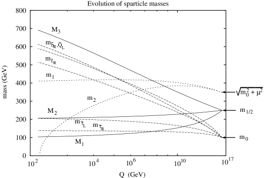
Figure 4: An example (from Ref. bbo2 ) of the running of the soft-supersymmetry breaking parameters with $Q$. The particle which feel the strong interaction are typically heavier than the non-colored ones, and the Higgs mass parameter $m_{2}^{2}$ is driven negative giving rise to breaking of the electroweak symmetry.

Minimizing the tree level Higgs potential $V_{0}$ one obtains the familiar tree-level conditions

$${1\over 2}M_{Z}^{2} = {{m_{H_{1}}^{2}-m_{H_{2}}^{2}\tan^{2}\beta}\over{\tan^{2}\beta-1}}-\mu^{2}\;,$$ (111)

and

$$B\mu = {1\over 2}(m_{H_{1}}^{2}+m_{H_{2}}^{2}+2\mu^{2})\sin 2\beta\;.$$ (112)

Notice that the signs of $B$ and $\mu$ are not determined by the minimization conditions giving rise to two distinct cases mentioned above.

Substituting Eq. (107) into Eq. (111) yields the result:

$$\mu^{2}+M_{Z}^{2}/2=m_{0}^{2}\left(1+\left(\frac{3}{2}{Y_{t}\over Y_{t}^{ir}}-1\right)\tan^{2}\beta\right)\frac{1}{\tan^{2}\beta-1}+$$

$$m_{1/2}^{2}\left(0.5-\left(0.5+{Y_{t}\over Y_{t}^{ir}}\left(-7+3{Y_{t}\over Y_{t}^{ir}}\right)\right)\tan^{2}\beta\right)\frac{1}{\tan^{2}\beta-1}.$$ (113)

Note in Eq. (107) that $m_{H_{2}}^{2}<0$, which is usually a sufficient condition to induce EWSB. For large $\tan\beta$, the Higgs mass parameters are more complicated. In the limit of $t-b$ Yukawa unification, they simplify to COPW2

$$m_{H_{1}}^{2}\simeq m_{H_{2}}^{2}\simeq{m_{0}^{2}}\left(1-\frac{9}{7}{Y_{t}\over Y_{t}^{ir}}\right)+m^{2}_{1/2}\left(0.5+{Y_{t}\over Y_{t}^{ir}}\left(-6+\frac{18}{7}{Y_{t}\over Y_{t}^{ir}}\right)\right),$$ (114)

and Eq. (113) must be modified accordingly. All of these relations are only approximate: the coefficients of $m_{1/2}$ depend on the exact values of $\alpha_{s}$ and the scale of the sparticle masses; the coefficients of $m_{0}$ and $A_{0}$ depend mainly on $\tan\beta$.

Given the mSUGRA boundary conditions, the RG equations give the values of the parameters in the Higgs potential $V_{0}$, and hence in the minimization conditions in Eqs. (111) and (112). The Higgs potential can depend strongly on the scale $Q$ at which it is evaluated. It was first argued in Ref. grz that this scale dependence resulting from the RG equations can be compensated by including the one-loop contributions to the Higgs potential. The one-loop effective potential is given by

$$V_{1} = V_{0}+\Delta V_{1}\;,$$ (115)

$$\Delta V_{1} = {1\over{64\pi^{2}}}{\rm Str}\left[{\cal M}^{4}\left(\ln{{{\cal M}^{2}}\over{Q^{2}}}-{3\over 2}\right)\right]\;,$$ (116)

is the one-loop contribution given in the dimensional reduction ($\overline{DR}$) renormalization schemedimred . The supertrace is defined as ${\rm Str}f({\cal M}^{2})=\sum_{i}C_{i}(-1)^{2s_{i}}(2s_{i}+1)f(m_{i}^{2})$ where $C_{i}$ is the color degrees of freedom and $s_{i}$ is the spin of the $i^{th}$ particle. To determine the minimum one must set the first derivatives of the effective potential to zero

$${{\partial V_{1}}\over{\partial\psi}}={{\partial V_{0}}\over{\partial\psi}}+{1\over{32\pi^{2}}}{\rm Str}\left[{{\partial{\cal M}^{2}}\over{\partial\psi}}{\cal M}^{2}\left(\ln{{{\cal M}^{2}}\over{Q^{2}}}-1\right)\right]=0\;.$$ (117)

One way to incorporate these corrections into the one-loop generalizations of Eqs. (111) and (112) is to set to zero the appropriate linear combinations of Higgs boson tadpole diagramsbbo2 . The corrections to the one-loop minimization conditions can then be completely written in terms of analytical formulas. Evaluated at the minimum of $V_{1}$, tadpole contributions involve the coupling $\partial{\cal M}^{2}/\partial\psi$ and the usual integration factor ${1\over{32\pi^{2}}}{\cal M}^{2}\left(\ln{{{\cal M}^{2}}\over{Q^{2}}}-1\right)$; setting tadpole contributions to zero is therefore equivalent to minimizing the potential.

The Higgs masses are given at tree-level by

$$M_{A}^{2} = m_{H_{1}}^{2}+m_{H_{2}}^{2}+2\mu^{2}\;,$$ (118)

$$M_{H,h}^{2} = {1\over 2}\left[M_{Z}^{2}+M_{A}^{2}\pm\sqrt{(M_{Z}^{2}+M_{A}^{2})^{2}-4M_{Z}^{2}M_{A}^{2}\cos^{2}2\beta}\right]\;,$$ (119)

$$M_{H^{\pm}}^{2} = M_{W}^{2}+M_{A}^{2}\;.$$ (120)

The one-loop corrections in Eq. (116) give corrections to the Higgs masses with the most important ones of order $m_{t}^{4}$CPeven .

In the MSSM, the Higgs potential is constrained by supersymmetry such that all tree-level Higgs boson masses and couplings are determined by just two independent parameters, commonly chosen to be the mass of the CP-odd pseudoscalar ($m_{A}$) and the ratio of vacuum expectation values (VEVs) of Higgs fields ($\tan\beta\equiv v_{2}/v_{1}$).

In the mSUGRA, mass of the CP-odd Higgs pseudoscalar ($m_{A}$) corresponding to the one loop effective potential has the following form:

$$m^{2}_{A} = (\tan\beta+\cot\beta)(B\mu+\Delta^{2}_{A}),$$

$$\Delta^{2}_{A} = \frac{3g^{2}}{32\pi^{2}}\frac{\mu A_{t}m^{2}_{t}}{M^{2}_{W}\sin^{2}\beta}\left[\frac{f(m^{2}_{\tilde{t}_{2}})-f(m^{2}_{\tilde{t}_{1}})}{m^{2}_{\tilde{t}_{2}}-m^{2}_{\tilde{t}_{1}}}\right]$$ (121)

$$+\frac{3g^{2}}{32\pi^{2}}\frac{\mu A_{b}m^{2}_{b}}{M^{2}_{W}\cos^{2}\beta}\left[\frac{f(m^{2}_{\tilde{b}_{2}})-f(m^{2}_{\tilde{b}_{1}})}{m^{2}_{\tilde{b}_{2}}-m^{2}_{\tilde{b}_{1}}}\right]$$

$$+\frac{g^{2}}{32\pi^{2}}\frac{\mu A_{\tau}m^{2}_{\tau}}{M^{2}_{W}\cos^{2}\beta}\left[\frac{f(m^{2}_{\tilde{\tau}_{2}})-f(m^{2}_{\tilde{\tau}_{1}})}{m^{2}_{\tilde{\tau}_{2}}-m^{2}_{\tilde{\tau}_{1}}}\right]\,,$$

where

$$f(m^{2})=m^{2}\left[\ln(\frac{m^{2}}{Q^{2}})-1\right]\,.$$ (122)

We suggest that the Higgs-boson masses and couplings should be calculated with leading one loop corrections not only from the top Yukawa interactions but also from the bottom and the tau Yukawa interactions in the one-loop effective potential CPeven , and should be evaluated at a scale close to $Q=\sqrt{m_{\tilde{t}_{L}}m_{\tilde{t}_{R}}}$ rge-Baer . With this scale choice, the numerical value of the CP-odd Higgs boson mass ($m_{A}$) at large $\tan\beta$ rge-Baer ; Madison is relatively insensitive to the exact scale and the loop corrections to $M_{A}$ are small compared to the ‘tree level’ contribution. In addition, when this high scale is used, the RGE improved one-loop corrections approximately reproduce the dominant two loop perturvative calculation of the mass of the lighter CP-even Higgs scalar ($m_{h}$). The numerical values of $m_{h}$ calculated at this scale can be very close to the results of Ref. Two-Loop where somewhat different scales higher than $M_{Z}$ have been adopted in evaluating the effective potential.

V Radiative Corrections to Particle Masses

V.1 Introduction

In this section, we present approximations for the one-loop supersymmetric radiative corrections to particle masses in the MSSM. These formulae have been tested in the mSUGRA model and are typically good to $1-2\%$. The calculations are performed in the dimensional reduction scheme where the supersymmetric Ward-Takahashi identities are ensured to at least the two-loop order. The divergences are removed by the (modified) minimal subtraction procedure, which we shall call the $\overline{\rm DR}$ scheme drscheme .

The full set of one-loop corrections and the approximations presented here can be found in Ref. BMPZ . We have changed some of the notation to conform with the SUGRA Working Group conventions. For example, we adopt the Working Group convention on the sign of $\mu$-parameter, and relabel $\tilde{t}_{1}$ to be the lighter top squark, etc. In some regions of the parameter space, these corrections can be important. We suggest them be included in event simulation programs such as the ISAJET z-isajet and the SPYTHIA spythia , which currently have only leading logarithmic contribution in RG evolutions.

We express the one-loop integrals for the self-energy diagrams in terms of the standard Passarino-Veltman functions PVfunc , which are defined as

$$A(m)=-i16\pi^{2}Q^{4-D}\int{d^{D}k\over(2\pi)^{D}}{1\over k^{2}-m^{2}}$$ (123)

$$B_{0}(p,m_{1},m_{2})=-i16\pi^{2}Q^{4-D}\int{d^{D}k\over(2\pi)^{D}}{1\over\left[k^{2}-m_{1}^{2}\right]\left[(k-p)^{2}-m_{2}^{2}\right]}$$ (124)

$$p_{\mu}B_{1}(p,m_{1},m_{2})=-i16\pi^{2}Q^{4-D}\int{d^{D}k\over(2\pi)^{D}}{k_{\mu}\over\left[k^{2}-m_{1}^{2}\right]\left[(k-p)^{2}-m_{2}^{2}\right]}$$ (125)

$$g_{\mu\nu}B_{22}(p,m_{1},m_{2})+p_{\mu}p_{\nu}B_{21}(p,m_{1},m_{2})=-i16\pi^{2}Q^{4-D}\int{d^{D}k\over(2\pi)^{D}}{k_{\mu}k_{\nu}\over\left[k^{2}-m_{1}^{2}\right]\left[(k-p)^{2}-m_{2}^{2}\right]}$$ (126)

where $Q$ is the renormalization scale. In certain limits, these functions have simple forms. For example, we shall take

$$B_{0}(0,m_{1},m_{2})=-\ln\left(M^{2}\over Q^{2}\right)+1+{m^{2}\over m^{2}-M^{2}}\ln\left(M^{2}\over m^{2}\right)\ ,$$ (127)

$$B_{1}(0,m_{1},m_{2})={1\over 2}\left[-\ln\left(M^{2}\over Q^{2}\right)+{1\over 2}+{1\over 1-x}+{\ln x\over(1-x)^{2}}-\theta(1-x)\ln x\right]\ ,$$ (128)

where $M=\max(m_{1},m_{2}),$ $m=\min(m_{1},m_{2}),$ $x=m_{2}^{2}/m_{1}^{2}$, and

$$B_{1}(p,0,m)=-{1\over 2}\ln\left({M^{2}\over Q^{2}}\right)+1-{1\over 2y}\left[1+{(y-1)^{2}\over y}\ln|y-1|\right]+{1\over 2}\theta(y-1)\ln y\ ,$$ (129)

where $M=\max(p^{2},m^{2})$ and $y=p^{2}/m^{2}$.

These formulae can also be used in an effective field theory approach to the particle masses. When the SUSY particles are heavy compared to the weak scale, it is appropriate to decouple them at an effective SUSY scale, $M_{\rm SUSY}$. Below $M_{\rm SUSY}$, the couplings should then be run in an effective theory which contains just the light SM particles. This is, in fact, the approach used by many groups RGrunning . Of course, in this approach, it is still necessary to include some enhanced finite threshold corrections. These corrections can be extracted from the following formulae by omitting the terms which contain logarithms of the renormalization scale.

V.2 Quark and lepton masses

The quark and lepton masses contain SM and SUSY radiative corrections. In some cases, they can be important or even dominant. The following approximations contain the most important contributions.

V.2.1 Top quark mass

The precise calculation of the running top quark mass has both theoretical and experimental significance. For example, radiative electroweak symmetry breaking and the radiative correction to the lightest Higgs boson mass both depend on the value of the running top quark mass, $m_{t}(Q)$. We found the following formula approximates the full one-loop radiative correction to about $\pm 1\%$,

$$M_{t}=m_{t}(Q)\left[1+\left({\Delta m_{t}\over m_{t}}\right)^{\rm QCD}+\left({\Delta m_{t}\over m_{t}}\right)^{\rm SUSY}\right]\ ,$$ (130)

where

$$\left({\Delta m_{t}\over m_{t}}\right)^{\rm QCD}={\alpha_{s}(Q)\over 3\pi}\left[3\ln\left({Q^{2}\over M_{t}^{2}}\right)+5\right]\ .$$ (131)

and BMPZ ; donini

$$\left({\Delta m_{t}\over m_{t}}\right)^{\rm SUSY} = -\ {\alpha_{s}(Q)\over 3\pi}\Bigg{\{}B_{1}(m_{t},m_{\tilde{g}},m_{\tilde{t}_{1}})+B_{1}(m_{t},m_{\tilde{g}},m_{\tilde{t}_{2}})$$

$$-{2m_{\tilde{g}}(A_{t}-\mu\cot\beta)\over m_{\tilde{t}_{1}}^{2}-m_{\tilde{t}_{2}}^{2}}\Bigg{[}B_{0}(m_{t},m_{\tilde{g}},m_{\tilde{t}_{1}})-B_{0}(m_{t},m_{\tilde{g}},m_{\tilde{t}_{2}})\Bigg{]}\Bigg{\}}\ .$$

The SUSY QCD contribution (LABEL:mtgluino) can be as large as the SM QCD contribution (131) for TeV-scale gluino and squark masses.

V.2.2 Bottom quark mass

Corrections to the bottom quark mass in the MSSM have received much attention because they can contain significant enhanced supersymmetric contributions in the region of large $\tan\beta$ bottomcorr . The best way to proceed is to first find the running bottom quark mass at $M_{Z}$ in the SM. This is related to running bottom quark mass at $M_{b}$ by the SM RG equations. At the two-loop level, one finds Gray

$$m_{b}(M_{b})^{\rm SM}=M_{b}\left[1+{5\alpha_{s}(M_{b})\over 3\pi}+12.4\left({\alpha_{s}(M_{b})\over\pi}\right)^{2}\right]^{-1}\ .$$ (133)

The running bottom quark mass at $M_{Z}$ in the MSSM is then

$$m_{b}(M_{Z})^{\rm MSSM}=m_{b}(M_{Z})^{\rm SM}\left[1-\left({\Delta m_{b}\over m_{b}}\right)^{\rm SUSY}\right]\ .$$ (134)

where

$$\left({\Delta m_{b}\over m_{b}}\right)^{\rm SUSY} = -\ {\alpha_{s}(M_{Z})\over 3\pi}\Bigg{\{}B_{1}(0,m_{\tilde{g}},m_{\tilde{b}_{1}})+B_{1}(0,m_{\tilde{g}},m_{\tilde{b}_{2}})$$ (135)

$$- {2m_{\tilde{g}}(A_{t}-\mu\tan\beta)\over m_{\tilde{b}_{1}}^{2}-m_{\tilde{b}_{2}}^{2}}\Bigg{[}B_{0}(0,m_{\tilde{g}},m_{\tilde{b}_{1}})-B_{0}(0,m_{\tilde{g}},m_{\tilde{b}_{2}})\Bigg{]}\Bigg{\}}$$

$$- {\lambda_{t}^{2}\over 16\pi^{2}}{\mu\ (A_{t}\tan\beta-\mu)\over m_{{\tilde{t}}_{1}}^{2}-m_{{\tilde{t}}_{2}}^{2}}\Bigg{[}B_{0}(0,\mu,m_{{\tilde{t}}_{1}})-B_{0}(0,\mu,m_{{\tilde{t}}_{2}})\Bigg{]}$$

$$- {g^{2}\over 16\pi^{2}}\Bigg{\{}{\mu M_{2}\tan\beta\over\mu^{2}-M_{2}^{2}}\Bigg{[}c_{t}^{2}B_{0}(0,M_{2},m_{{\tilde{t}}_{1}})+s_{t}^{2}B_{0}(0,M_{2},m_{{\tilde{t}}_{2}})\Bigg{]}+(\mu\leftrightarrow M_{2})\Bigg{\}}\ ,$$

where $s_{t}=\sin\theta_{\tilde{t}}$ and $c_{t}=\cos\theta_{\tilde{t}}$. The angle $\theta_{\tilde{t}}$ is the mixing angle of the top squark mass-squared matrix, and satisfies

$$\sin 2\theta_{\tilde{t}}={2m_{t}(A_{t}-\mu\cot\beta)\over m^{2}_{{\tilde{t}}_{1}}-m^{2}_{{\tilde{t}}_{2}}}\ .$$ (136)

V.2.3 Tau lepton mass

The SUSY corrections to the tau lepton mass are also enhanced in the large $\tan\beta$ region. To find the correction, we proceed as before, and first use the SM RG equations and radiative correction to find the running tau lepton mass, $m_{\tau}(M_{Z})^{\rm SM}$, at the scale $M_{Z}$. This is related to the running tau lepton mass in the MSSM as follows,

$$m_{\tau}(M_{Z})^{\rm MSSM}=m_{\tau}(M_{Z})^{\rm SM}\left[1-\left({\Delta m_{\tau}\over m_{\tau}}\right)^{\rm SUSY}\right]\ .$$ (137)

where

$$\left({\Delta m_{\tau}\over m_{\tau}}\right)^{\rm SUSY}=-\ {g^{2}\over 16\pi^{2}}{\mu M_{2}\tan\beta\over\mu^{2}-M_{2}^{2}}\Bigg{[}B_{0}(0,M_{2},m_{\tilde{\nu}_{\tau}})-B_{0}(0,\mu,m_{\tilde{\nu}_{\tau}})\Bigg{]}\ .$$ (138)

V.3 Supersymmetric particle masses

V.3.1 Gluino mass

The gluino mass corrections arise from gluon/gluino and quark/squark loops PP1 ; donini . The corrections can be rather large, so we include them in a way which automatically incorporates the one-loop renormalization group resummation,

$$m_{\tilde{g}}\ =\ M_{3}(Q)\left[1-{3\alpha_{s}(Q)\over 4\pi}\left(5+3\ln\left({Q^{2}\over M_{3}^{2}}\right)-4B_{1}(M_{3},0,M_{\widetilde{Q}_{1}})\right)\right]^{-1}\ .$$ (139)

We have approximated all squark masses by a common mass $M_{\widetilde{Q}_{1}}$, which is the soft mass of the first generation of left-handed squarks.

V.3.2 Neutralino and chargino masses

The complete set of corrections to the neutralino and chargino masses is very involved PP1 ; neucharcorr ; BMPZ . In the following we will present approximation formulae which typically work to better than $2\%$. We shall assume $|\mu|\,>\,M_{1},M_{2},M_{Z},$ which is correct in the mSUGRA and minimal gauge-mediated models, with radiative breaking of the electroweak symmetry. This approximation leads to an error of order $(\alpha/4\pi)M^{2}_{Z}/\mu^{2}$ in the masses.

The one-loop radiatively corrected neutralino/chargino masses are determined from their tree-level running masses by

$$M_{i}=M_{i}(Q)\biggl{[}1+\left({\Delta M_{i}\over M_{i}}\right)\biggr{]}\ ,$$ (140)

where $i$ labels the different species of neutralinos and charginos.

For $i=\widetilde{\chi}^{0}_{1}$, we find

$$\left({\Delta M_{i}\over M_{i}}\right) = {g^{\prime 2}\over 32\pi^{2}}\biggl{\{}11\theta_{M_{1}M_{\widetilde{Q}_{1}}}+9\theta_{M_{1}M_{\widetilde{L}_{1}}}+\theta_{M_{1}\mu M_{Z}}-2B_{1}(0,\mu,m_{A})$$ (141)

$$-{2\mu\over M_{1}}\sin(2\beta)\biggl{(}B_{0}(0,\mu,0)-B_{0}(0,\mu,m_{A})\,\biggr{)}-{23\over 2}\biggr{\}}\ ,$$

where $\theta_{m_{1}\ldots m_{2}}\equiv\ln(M^{2}/Q^{2})$ with $M^{2}={\rm max}(m_{1}^{2},...,m_{2}^{2})$. We have approximated the tree-level mass of $\widetilde{\chi}^{0}_{1}$ by $M_{1}$, and the squark and slepton masses by the first generation left-handed soft masses $M_{\widetilde{Q}_{1}}$ and $M_{\widetilde{L}_{1}}$.

For $i=\widetilde{\chi}^{0}_{2}$ and $\widetilde{\chi}^{+}_{1}$, we find

$$\left({\Delta M_{i}\over M_{i}}\right) = {g^{2}\over 32\pi^{2}}\bigg{\{}9\theta_{M_{2}M_{\widetilde{Q}_{1}}}+3\theta_{M_{2}M_{\widetilde{L}_{1}}}+\theta_{M_{2}\mu M_{Z}}-12\theta_{M_{2}M_{W}}-\theta(M_{W}-M_{2})\left(12.56{M_{2}\over M_{W}}-14.80\right)$$

$$+\theta(M_{2}-M_{W})\left[4.32\ln\left({M_{2}\over M_{W}}-0.8\right)+9.20\right]$$

$$-2B_{1}(0,\mu,m_{A})-{2\mu\over M_{2}}\sin(2\beta)\bigg{(}B_{0}(0,\mu,0)-B_{0}(0,\mu,m_{A})\bigg{)}-{15\over 2}\biggr{\}}\ ,$$

where we have approximated the tree-level masses of $\widetilde{\chi}^{0}_{2}$ and $\widetilde{\chi}^{+}_{1}$ by $M_{2}$.

For $i=\widetilde{\chi}^{0}_{3},\ \widetilde{\chi}^{0}_{4}$ and $\widetilde{\chi}^{+}_{2}$, we find

$$\left({\Delta M_{i}\over M_{i}}\right) = -\ {3\over 32\pi^{2}}\bigg{[}(\lambda_{b}^{2}+\lambda_{t}^{2})B_{1}(\mu,0,M_{\widetilde{Q}_{3}})+\lambda_{t}^{2}B_{1}(\mu,0,M_{\widetilde{U}_{3}})$$ (143)

$$\qquad\qquad+\lambda_{b}^{2}B_{1}(\mu,0,M_{\widetilde{D}_{3}})\bigg{]}$$

$$\ +{3g^{2}\over 64\pi^{2}}\bigg{[}{1\over 2}\theta_{\mu M_{2}M_{Z}}-3\theta_{\mu M_{Z}}-B_{1}(\mu,0,m_{A})+4\bigg{]}\ ,$$

where we have approximated the tree-level masses of $\widetilde{\chi}^{0}_{3,4}$ and $\widetilde{\chi}^{+}_{2}$ by $|\mu|$, and $M_{{\widetilde{Q}_{3}},{\widetilde{U}_{3}},{\widetilde{D}_{3}}}$ denote the third generation soft squark masses.

V.3.3 Squark masses

The dominant corrections to the first two generation and the bottom squark masses come from SUSY QCD 12squarkcorr . For these cases, the one-loop radiative corrections are given by

$$m_{\tilde{q}}^{2}=m_{\tilde{q}}^{2}(Q)\left[1+{2\alpha_{s}(Q)\over 3\pi}\bigg{\{}1+3x+(x-1)^{2}\ln|x-1|-x^{2}\ln x\ +2x\ln\left({Q^{2}\over m_{\tilde{q}}^{2}}\right)\bigg{\}}\right]\ ,$$ (144)

where $x=m_{\tilde{g}}^{2}/m_{\tilde{q}}^{2}$.

The radiative corrections to the top squark mass need a more careful treatment donini ; BMPZ because the off-diagonal element of the top squark mass-squared matrix is proportional to the top quark mass. The full one-loop formulae for the top squark mass are very involved. We present here approximations which work for the cases of light and heavy top squarks. To make the approximations as good as possible, we use a matrix formalism in which the top squark mass-squared matrix has the form:

$${\cal M}_{\tilde{t}}^{2}={\cal M}_{\tilde{t}}^{2}(Q)\ +\pmatrix{\Delta M^{2}_{LL}&\Delta M^{2}_{LR}\cr\Delta M^{2}_{LR}&\Delta M^{2}_{RR}}\ ,$$ (145)

where the $\Delta M^{2}$ entries are as follows:

$$\Delta M^{2}_{LL} = {2\alpha_{s}\over 3\pi}\bigg{\{}2m_{{\tilde{t}}_{1}}^{2}\left[s_{t}^{2}B_{1}(m_{{\tilde{t}}_{1}},m_{{\tilde{t}}_{2}},0)+c_{t}^{2}B_{1}(m_{{\tilde{t}}_{1}},m_{{\tilde{t}}_{1}},0)\right]$$ (146)

$$\qquad+A_{0}(m_{\tilde{g}})+A_{0}(m_{t})-(m_{{\tilde{t}}_{1}}^{2}-m_{\tilde{g}}^{2}-m_{t}^{2})B_{0}(0,m_{\tilde{g}},m_{t})\bigg{\}}$$

$$-{1\over 16\pi^{2}}\bigg{[}\lambda_{t}^{2}c_{t}^{2}A_{0}(m_{{\tilde{t}}_{2}})+\lambda_{b}^{2}A_{0}(m_{\tilde{b}})$$

$$\qquad-2(\lambda_{t}^{2}+\lambda_{b}^{2})A_{0}(\mu)+(\lambda_{t}^{2}c_{\beta}^{2}+\lambda_{b}^{2}s_{\beta}^{2})A_{0}(m_{A})\bigg{]}$$

$$-{\lambda_{t}^{2}\over 32\pi^{2}}\bigg{[}\Lambda(\theta_{t},\beta)B_{0}(0,m_{{\tilde{t}}_{2}},m_{A})+\Lambda(\theta_{t}-{\pi\over 2},\beta)B_{0}(0,0,m_{A})$$

$$\qquad+\Lambda(\theta_{t},\beta-{\pi\over 2})B_{0}(0,m_{{\tilde{t}}_{2}},0)+\Lambda(\theta_{t}-{\pi\over 2},\beta-{\pi\over 2})B_{0}(m_{{\tilde{t}}_{1}},m_{{\tilde{t}}_{1}},m_{Z})\bigg{]}$$

$$-{1\over 16\pi^{2}}\bigg{[}\left(\lambda_{t}^{2}m_{t}^{2}c_{\beta}^{2}+\lambda_{b}^{2}(\mu c_{\beta}+A_{b}s_{\beta})^{2}\right)B_{0}(0,m_{\tilde{b}},m_{A})$$

$$\qquad+\left(\lambda_{t}^{2}m_{t}^{2}s_{\beta}^{2}+\lambda_{b}^{2}(\mu s_{\beta}-A_{b}c_{\beta})^{2}\right)B_{0}(0,m_{\tilde{b}},0)\bigg{]}$$

$$\Delta M^{2}_{LR} = \ {2\alpha_{s}\over 3\pi}c_{t}s_{t}\left[(m_{{\tilde{t}}_{1}}^{2}+m_{{\tilde{t}}_{2}}^{2})B_{0}(m_{{\tilde{t}}_{1}},m_{{\tilde{t}}_{2}},0)+2m_{{\tilde{t}}_{1}}^{2}B_{0}(m_{{\tilde{t}}_{1}},m_{{\tilde{t}}_{1}},0)\right]$$ (147)

$$-{4\alpha_{3}\over 3\pi}m_{t}m_{\tilde{g}}B_{0}(0,m_{t},m_{\tilde{g}})+{3\lambda_{t}^{2}\over 16\pi^{2}}c_{t}s_{t}A_{0}(m_{{\tilde{t}}_{2}})$$

$$-{\lambda_{t}^{2}\over 32\pi^{2}}\bigg{[}\Omega(\theta_{t},\beta)B_{0}(0,m_{{\tilde{t}}_{2}},m_{A})+\Omega(-\theta_{t},\beta)B_{0}(0,0,m_{A})$$

$$\qquad+\Omega(\theta_{t},{\pi\over 2}+\beta)B_{0}(0,m_{{\tilde{t}}_{2}},0)+\Omega(-\theta_{t},{\pi\over 2}+\beta)B_{0}(m_{{\tilde{t}}_{1}},m_{{\tilde{t}}_{1}},M_{Z})\bigg{]}$$

$$-{1\over 16\pi^{2}}\bigg{[}\biggl{(}\lambda_{t}^{2}m_{t}c_{\beta}(\mu s_{\beta}+A_{t}c_{\beta})+\lambda_{b}^{2}m_{t}s_{\beta}(\mu c_{\beta}+A_{b}s_{\beta})\biggr{)}B_{0}(0,m_{\tilde{b}},m_{A})$$

$$\qquad-\lambda_{t}^{2}m_{t}s_{\beta}(\mu c_{\beta}-A_{t}s_{\beta})B_{0}(0,m_{\tilde{b}},0)\bigg{]}$$

$$\Delta M^{2}_{RR} = {2\alpha_{s}\over 3\pi}\bigg{\{}2m_{{\tilde{t}}_{1}}^{2}\left[c_{t}^{2}B_{1}(m_{{\tilde{t}}_{1}},m_{{\tilde{t}}_{2}},0)+s_{t}^{2}B_{1}(m_{{\tilde{t}}_{1}},m_{{\tilde{t}}_{1}},0)\right]$$ (148)

$$\qquad+A_{0}(m_{\tilde{g}})+A_{0}(m_{t})-(m_{{\tilde{t}}_{1}}^{2}-m_{\tilde{g}}^{2}-m_{t}^{2})B_{0}(0,m_{\tilde{g}},m_{t})\bigg{\}}$$

$$-{\lambda_{t}^{2}\over 16\pi^{2}}\left[s_{t}^{2}A_{0}(m_{{\tilde{t}}_{2}})+A_{0}(m_{\tilde{b}})-4A_{0}(\mu)+2c_{\beta}^{2}A_{0}(m_{A})\right]$$

$$-{\lambda_{t}^{2}\over 32\pi^{2}}\bigg{[}\Lambda({\pi\over 2}-\theta_{t},\beta)B_{0}(0,m_{{\tilde{t}}_{2}},m_{A})+\Lambda(-\theta_{t},\beta)B_{0}(0,0,m_{A})$$

$$\qquad+\Lambda({\pi\over 2}-\theta_{t},\beta-{\pi\over 2})B_{0}(0,m_{{\tilde{t}}_{2}},0)+\Lambda(-\theta_{t},\beta-{\pi\over 2})B_{0}(m_{{\tilde{t}}_{1}},m_{{\tilde{t}}_{1}},m_{Z})\bigg{]}$$

$$-{1\over 16\pi^{2}}\bigg{[}\left(\lambda_{b}^{2}m_{t}^{2}s_{\beta}^{2}+\lambda_{t}^{2}(\mu s_{\beta}+A_{t}c_{\beta})^{2}\right)B_{0}(0,m_{\tilde{b}},m_{A})$$

$$\qquad+\lambda_{t}^{2}(\mu c_{\beta}-A_{t}s_{\beta})^{2}B_{0}(0,m_{\tilde{b}},0)\bigg{]}\ ,$$

with $s_{\beta}=\sin\beta$ and $c_{\beta}=\cos\beta$. We have defined the two functions

$$\Lambda(\theta_{t},\beta) = \left(2m_{t}\cos\beta\sin\theta_{t}-(\mu\sin\beta+A_{t}\cos\beta)\cos\theta_{t}\right)^{2}$$ (149)

$$\qquad+(\mu\sin\beta+A_{t}\cos\beta)^{2}\cos^{2}\theta_{t}$$

$$\Omega(\theta_{t},\beta) = -2m_{t}^{2}\cos^{2}\beta\sin 2\theta_{t}+2m_{t}\cos\beta(\mu\sin\beta+A_{t}\cos\beta)\ .$$ (150)

The eigenvalues of the mass-squared matrix (145) determine the one-loop radiatively corrected top squark masses.

V.3.4 Slepton masses

The corrections to the slepton masses are small in the mSUGRA model. We find that the corrections to the electron or muon slepton masses are typically in the range $\pm(1-2)\%$, as are the (predominantly) left- and right-handed tau slepton corrections. In the gauge-mediated model, tau slepton can receive appreciable corrections at large $\tan\beta$.

V.3.5 Higgs boson masses

The Higgs sector of the MSSM is composed of five physical Higgs bosons. Generically, one of them ($h^{0}$) is light while the other four ($H^{0},A^{0}$ and ${H^{\pm}}$) are heavy. In the decoupling limit where $m_{A}\rightarrow\infty$, the lightest Higgs boson $h^{0}$ becomes indistinguishable from that of the SM.

The radiative corrections to the lightest CP-even Higgs-boson mass are extremely important and have been extensively studied by many groups lighthiggscorr ; 2loopcorr . The most important contributions come from an incomplete cancellation of the quark and squark loops. Interested readers should consult summaries by the LEP2 Higgs boson working group and by Haber lephiggs for the one-loop formulae and some further refinements. The corrections to the other heavy Higgs boson masses, $m_{A}$, $m_{H^{\pm}}$ and $m_{H}$, are typically less than 1% heavyhiggscorr .

V.4 Summary

Radiative corrections are very important for a precise determination of the SUSY parameters in the mSUGRA and gauge mediated models. We have surveyed the radiative corrections to the SM and SUSY particle masses and presented a series of useful approximations. These formulae include one-loop leading logarithmic corrections as well as potentially large finite contributions.

VI Radiative Corrections to Couplings and Superoblique Parameters

VI.1 Soft vs. Hard SUSY-breaking

If supersymmetry (SUSY) were an exact symmetry of nature, the properties of supersymmetric particles would be completely determined by the properties of their standard model partners. For example, their masses would satisfy the relations

$$m_{\tilde{f}}=m_{f}\ ,$$ (151)

where $m_{\tilde{f}}$ and $m_{f}$ are the masses of supersymmetric particles and their standard model partners, respectively. As is well known, relations between dimensionful parameters such as Eq. (151) are broken via the introduction of soft SUSY-breaking parameters. These soft terms are free parameters of SUSY theories, and their a priori arbitrariness is responsible for the lack of predictability of SUSY for collider experiments.

In addition to these relations, however, SUSY also predicts the equivalence of dimensionless couplings. By dimensional arguments, these identities cannot be broken by soft SUSY-breaking parameters at tree level and are therefore known as “hard SUSY relations” Hikasa . For example, supersymmetry implies

$$g_{i}=h_{i}\ ,$$ (152)

where $g_{i}$ are the standard model gauge couplings, $h_{i}$ are their supersymmetric analogues, the gaugino-fermion-sfermion couplings, and the subscript $i=1,2,3$ refers to the U(1), SU(2), and SU(3) gauge groups, respectively. In contrast to other predictions, such as the universality of scalar or gaugino masses, hard SUSY relations are independent of the SUSY-breaking mechanism, and are therefore valid in all supersymmetric theories. The verification of hard SUSY relations provides the only model-independent method of quantitatively confirming that newly-discovered particles are indeed superpartners FMPT . At lepton colliders, hard SUSY relations have been demonstrated to be verifiable at the percent level for many scenarios through a variety of processes FMPT ; NFT ; gex ; NPY ; KNPY , as will be discussed below. (At hadron colliders, the possible scenarios are far more numerous and much less well-studied. Such hadron collider studies are harder to do because several slepton signals may be involved and the backgrounds are more complex.)

VI.2 Radiative Corrections to Couplings

The relations of Eq. (152) are valid at tree-level. However, in the presence of soft SUSY-breaking, radiative corrections violate Eq. (152) and lead to “hard SUSY-breaking.” The radiative corrections may be most easily understood in the language of renormalization group equations. Consider a simplified model with some scalar superparticles at a heavy mass scale $M$ and all other particles at a light mass scale $m$, typically taken to be the weak scale. Above the scale $M$, SUSY is unbroken, and we have $h_{i}=g_{i}$. Below $M$, where the heavy superpartners decouple, light fermion loops still renormalize the gauge boson wavefunction (and thus, $g_{i}$) but heavy sfermion loops and sfermion-fermion loops decouple from gauge boson and gaugino wavefunction renormalization, respectively C . (Gauge loops still renormalize both wavefunctions in the non-Abelian case.) Since not all loops involving the scalar and fermion fields of each supermultiplet decouple simultaneously, supersymmetry is broken in the gauge sector, and therefore the gauge couplings $g_{i}$ and gaugino couplings $h_{i}$ evolve differently between the scales $M$ and $m$. The splitting between $h_{i}$ and $g_{i}$ at the light scale is given by

$$\widetilde{U}_{i}\equiv\frac{h_{i}(m)}{g_{i}(m)}-1\approx\frac{g_{i}^{2}(m)}{16\pi^{2}}\Delta b_{i}\ln\frac{M}{m}\ ,$$ (153)

where $i=1,2,3$ denotes the gauge group as before, and $\Delta b_{i}$ is the one-loop $\beta$-function coefficient contribution from all light particles whose superpartners are heavy. The coupling splittings may also receive contributions from split exotic supermultiplets, such as the messenger supermultiplets of gauge-mediated SUSY-breaking theories gth ; KRS .

Equation (153) has a number of interesting properties. In particular, although the splittings between $h_{i}$ and $g_{i}$ are one-loop effects, they can be greatly enhanced for large heavy sectors (large $\Delta b_{i}$) and large mass splittings (large $M/m$). The corrections of Eq. (153) are just a subset of all one-loop corrections. However, because of these enhancements, these splittings are in many cases the dominant effects, as has been demonstrated through complete one-loop calculations KNPY . Note that the fact that they grow with $\ln\frac{M}{m}$ implies that these effects are non-decoupling, that is, they are in principle sensitive to particles with arbitrarily high mass, in contrast to many other observables. Note also that the coupling $h_{i}$ is more asymptotically free than $g_{i}$, $h_{i}(m)>g_{i}(m)$, and so the parameters $\widetilde{U}_{i}$ are always positive (at the leading log level).

VI.3 Superoblique Parameters

The hard SUSY-breaking corrections have a beautiful analogy to the oblique corrections of the electroweak sector of the standard model:

• In the standard model, SU(2) multiplets with custodial SU(2)-breaking masses, such as the $(t,b)$ multiplet, renormalize the propagators of the $(W,Z)$ vector multiplet differently, leading to explicit custodial SU(2)-breaking in the vector multiplet at the quantum level, and introducing non-decoupling effects that grow with the mass splitting.

• In supersymmetric models, supermultiplets with soft SUSY-breaking masses, such as the $(\tilde{f},f)$ supermultiplet, renormalize the propagators of the $(\hbox{gauge boson},\hbox{gaugino})$ vector supermultiplet differently, leading to explicit SUSY-breaking in the vector supermultiplet at the quantum level, and introducing non-decoupling effects that grow with the mass splitting.

On the strength of this analogy, hard SUSY-breaking corrections have been dubbed “super-oblique corrections” in Ref. gth , and the parameters $\widetilde{U}_{i}$, which are most analogous to the wavefunction renormalization oblique parameter $U$ PT , are called “superoblique parameters.” Further details concerning this analogy may be found in Refs. gth ; NPY ; KRS .

VI.4 Experimental Implications of Superoblique Parameters

Superoblique parameters have relevance for experimental studies in many ways. Among these are the following:

• Superoblique corrections influence superparticle production rates and branching ratios, which depend on the couplings $h_{i}$ and therefore the superoblique parameters $\widetilde{U}_{i}$.

• As noted above, the verification of hard SUSY relations (with their superoblique corrections) allows us to quantitatively determine whether newly-discovered particles are in fact supersymmetric. If these particles are determined to be supersymmetric, verifications of hard SUSY relations will play an important part in establishing the underlying supersymmetry of the couplings.

• Perhaps most exciting, if new particles are determined to be supersymmetric, small but unexplained violations of hard SUSY relations will provide unambiguous evidence for as-yet-undiscovered SUSY particles. If portions of the SUSY spectrum are beyond the reach of colliders, the non-decoupling superoblique parameters may provide indirect experimental evidence for superparticles with arbitrarily high masses (if they belong to highly split supermultiplets).

With regard to the last point, it is worth noting that fine-tuning arguments place stringent upper bounds only on sfermions that couple strongly to the Higgs boson, namely, the 3rd generation squarks finetune ; 211 . The squarks and sleptons of the 1st and 2nd generations may have masses far beyond the reach of the Tevatron and even the LHC, and in fact, such massive squarks and sleptons provide an elegant solution to the SUSY flavor problem by naturally suppressing dangerous contributions to, for example, $K^{0}-\bar{K}^{0}$ mixing and $\mu\to e\gamma$ 211 ; 212 . In such models, mass hierarchies of order $M/m\sim 40-200$ are possible.

The numerical values of the superoblique parameters $\widetilde{U}_{i}$ for two representative models are given in Table 3. We find that fractional splittings of several percent are possible, depending logarithmically on the mass hierarchy $M/m$.

Table 3: The superoblique parameters $\widetilde{U}_{i}$ in two representative models: “2–1 Models,” with all first and second generation sfermions at the heavy scale $M$, and “Heavy QCD Models,” with all squarks and gluinos at the heavy scale.

	$\widetilde{U}_{1}$	$\widetilde{U}_{2}$	$\widetilde{U}_{3}$
2–1 Models	$0.35\%\times\ln\frac{M}{m}$	$0.71\%\times\ln\frac{M}{m}$	$2.5\%\times\ln\frac{M}{m}$
Heavy QCD Models	$0.29\%\times\ln\frac{M}{m}$	$0.80\%\times\ln\frac{M}{m}$	—

VI.5 Measurements at Colliders

The experimental observables that are dependent on superoblique parameters have been exhaustively categorized in Ref. gex for both lepton and hadron colliders. The most promising observables at colliders are cross sections and branching ratios involving gauginos, and several of these possibilities have been examined in detailed studies. The results are, of course, highly dependent on the underlying SUSY parameters realized in nature, but we present a brief synopsis below.

• Measurements of $\widetilde{U}_{1}$. Selectron pair production at electron colliders includes a contribution from $t$-channel gaugino exchange. In particular, the reaction $e^{+}e^{-}\to\tilde{e}_{R}^{+}\tilde{e}_{R}^{-}$ depends on the $\tilde{B}$-$e$-$\tilde{e}$ coupling $h_{1}$, and has been studied in Ref. NFT . Under the assumption that the selectrons decay through $\tilde{e}\to\tilde{B}e$, the selectron and gaugino masses may be measured through kinematic endpoints. Combining this information with measurements of the differential cross section, $\widetilde{U}_{1}$ may be determined to ${\cal O}(1\%)$ with $20\hbox{ fb}^{-1}$ of data at $\sqrt{s}=500\hbox{ GeV}$.

  This high precision measurement may be further improved by considering the process $e^{-}e^{-}\to\tilde{e}_{R}^{-}\tilde{e}_{R}^{-}$. This process is made possible by the Majorana nature of gauginos. Relative to the $e^{+}e^{-}$ process, this reaction benefits from large statistics for typical SUSY parameters and extremely low backgrounds, especially if the electron beams are right-polarized. Depending on experimental systematic errors, determinations of $\widetilde{U}_{1}$ at the level of $0.3\%$ may be possible with integrated luminosities of $50\hbox{ fb}^{-1}$ gex .

• Measurements of $\widetilde{U}_{2}$. Chargino pair production has a dependence on $\widetilde{U}_{2}$ at lepton colliders through the $\tilde{\nu}$ exchange amplitude. This process was first studied as a way to verify hard SUSY relations in Ref. FMPT . In Ref. gex , estimates of 2–3% uncertainties for $\widetilde{U}_{2}$ were obtained from pair production of 172 GeV charginos with $\sqrt{s}=400-500\hbox{ GeV}$. In Ref. KNPY , these estimates were found to be conservative in the sense that these measurements are improved in most other regions of parameter space.

  The process $e^{+}e^{-}\to\tilde{\nu}_{e}\tilde{\nu}_{e}^{*}$ also depends on $\widetilde{U}_{2}$ through the $t$-channel chargino exchange amplitude. With a data sample of $100\hbox{ fb}^{-1}$, $\widetilde{U}_{2}$ may be determined to $\sim 0.6\%$ NPY .

• Measurements of $\widetilde{U}_{3}$. Finally, the superoblique parameter $\widetilde{U}_{3}$ may be measured through processes involving squarks. Squark pair production cross sections at lepton colliders are independent of superoblique corrections, but three-body production processes, such as $\tilde{t}t\tilde{g}$ and $\tilde{b}b\tilde{g}$ have been suggested as a probe gex ; KRS .

  Squark branching ratios may also sensitive to superoblique corrections if there are two or more competing modes. In Ref. gex , parameters were studied in which the two decays $\tilde{b}_{L}\to b\tilde{g}$ and $\tilde{b}_{L}\to b\tilde{W}$ were open. For parameters where the gluino decay is suppressed by phase space, these modes may be competitive, and measurements of the branching ratios yield constraints on $\widetilde{U}_{3}$. For example, for $m_{\tilde{b}_{L}}=300\hbox{ GeV}$, $\tilde{b}_{L}$ pair production at a $\sqrt{s}=1\hbox{ TeV}$ collider with integrated luminosity $200\hbox{ fb}^{-1}$ yields measurements of $\widetilde{U}_{3}$ at or below the 5% level for $10\hbox{ GeV}\mathrel{\raisebox{-2.58334pt}{$\stackrel{{\scriptstyle\textstyle<}}{{\sim}}$}}m_{\tilde{b}_{L}}-m_{\tilde{g}}\mathrel{\raisebox{-2.58334pt}{$\stackrel{{\scriptstyle\textstyle<}}{{\sim}}$}}100\hbox{ GeV}$. While these measurements are typically numerically less stringent than those discussed above, the SU(3) superoblique correction is typically large and so merits attention. In addition, the possibility of studying squark branching ratios is one that has particular promise at hadron colliders.

VII Supersymmetric Corrections to Standard Model Processes

VII.1 Introduction

The upgraded Tevatron collider will provide a wealth of new information. The data and analyses will shed new light on many aspects of the Standard Model, and may even include direct discoveries of physics beyond the Standard Model. For example, if low energy supersymmetry exists, supersymmetric particles might be discovered through their direct production and decay processes. Alternatively, new physics scenarios might be indirectly observed, constrained or excluded via virtual corrections to Standard Model processes. In this report we will discuss the implications of virtual supersymmetric corrections to various Standard Model processes in light of the expected measurements at the upgraded Tevatron collider. In the next section we discuss the supersymmetric radiative corrections to the top quark pair production cross section. In Section VII.3 we discuss single top quark production, and in Section VII.4 we discuss di-boson production. We summarize the report in the last section.

VII.2 Top quark pair production

The upgraded Tevatron, with center-of-mass energy 2 TeV and total integrated luminosity 2 (10) fb^-1, will produce approximately $10^{4}$ ($7\times 10^{4}$) top quark pairs. This should yield a measurement of the cross-section to a precision of about 12% (5.5%) TeV2000 .

The supersymmetric QCD (SQCD) corrections to the top quark pair production cross section were first considered in Refs. LHYH ; KLNR .Those papers did not include the full set of corrections. The calculation was completed for the case of degenerate squark masses by including the gluon self energy and box diagram contributions in Ref. Alam . A relative sign between the two box diagram contributions was corrected in Ref. ZS , and the overall sign of the box diagram contribution was corrected in Ref. DW . The SQCD correction to the cross section depends crucially on the box diagram contribution. With the correct sign the box diagram contribution largely cancels against the vertex correction, so that the total SQCD correction is less than 7% with a 200 GeV gluino mass and a 100 GeV degenerate squark mass DW . If both the gluino and squark masses are above 200 GeV, the total SQCD correction varies between 0 and $-3\%$. Such small corrections will not be discernible at the Tevatron upgrade. Below the anomalous threshold ($m_{\tilde{g}}^{2}+m_{\tilde{t}}^{2}<m_{t}^{2}$), the SQCD correction is greater than $+15\%$ ZSERR . However, the current lower bounds on the gluino and top squark masses are close to ruling out this region. If there is a large hierarchy between the two top squark masses, and the top squark mixing is large, the correction can be as large as $\pm 7\%$. Such a correction could be observed at the upgraded Tevatron with sufficient luminosity, if the standard theoretical uncertainty (from scale uncertainty, parton distribution functions, etc.) is not too large.

The SUSY electroweak-like (SEW) corrections to the top quark pair production cross-section have also been computed KLNR ; ttmssm . As one would expect, these corrections are typically small, of order a few percent. The SEW corrections can be enhanced in a couple of ways. If one of the top squarks is light (i.e. below 100 GeV), the light chargino is Higgsino-like, and $\tan\beta$ is very small and very large (e.g. $\tan\beta=0.7$ and 50) these corrections can reach about $-5.8\%$ and $-4.3\%$, respectively, at the Tevatron collider. Alternatively, the SEW corrections can be enhanced if the resonant condition $m_{t}=m_{\tilde{t}}+m_{\tilde{\chi}^{0}}$ is close to being met. In this case the SEW correction can be as large as $-30\%$ ($-15\%$) with $\tan\beta=0.7(\lower 3.01385pt\hbox{$\;\stackrel{{\scriptstyle\textstyle>}}{{\sim}}\;$}1.4)$. If the MSSM parameters are such that such a large enhancement occurs, the correction will be observable at the Tevatron upgrade, even with 2 fb^-1 integrated luminosity. It should be noted, however, that in these cases direct production of the light top squark will likely be observable as well.

MSSM loop-induced parity violating asymmetries in the strong production of polarized top quark pairs has also been investigated, both at the Tevatron ZS ; DW ; ttsm ; Chung ; LOYY ; Doreen and the LHC Doreen . In addition to the small SM contribution ttsm induced by diagrams involving the $Z$, the $W^{+}$, and the Goldstone boson $G^{+}$, the parity violating asymmetries in the MSSM are generated by diagrams involving the charged Higgs boson ($H^{\pm}$), the charginos ($\tilde{\chi}^{\pm}_{i}$) and the neutralinos ($\tilde{\chi}^{0}_{i}$). Since QCD preserves parity, parity violating asymmetries in the strong production of left- and right-handed top quark pairs can only arise beyond leading order in perturbation theory. We consider

• the differential left-right asymmetry

  $$\delta{\cal A}_{LR}(M_{t\bar{t}})=\frac{d\sigma_{{+\frac{1}{2},-\frac{1}{2}}}/dM_{t\bar{t}}-d\sigma_{{-\frac{1}{2},+\frac{1}{2}}}/dM_{t\bar{t}}}{d\sigma_{{+\frac{1}{2},-\frac{1}{2}}}/dM_{t\bar{t}}+d\sigma_{{-\frac{1}{2},+\frac{1}{2}}}/dM_{t\bar{t}}}\;,$$ (154)

  with $d\sigma_{\lambda_{t},\lambda{\bar{t}}}/dM_{t\bar{t}}$ denoting the invariant mass distribution of the polarized top quark pair,

• the integrated left-right asymmetry

  $${\cal A}_{LR}=\frac{\sigma_{{+\frac{1}{2},-\frac{1}{2}}}-\sigma_{{-\frac{1}{2},+\frac{1}{2}}}}{\sigma_{{+\frac{1}{2},-\frac{1}{2}}}+\sigma_{{-\frac{1}{2},+\frac{1}{2}}}}~{},$$ (155)

• and the integrated left-right asymmetry assuming that the antitop quark polarization is not measured in the experiment

  $${\cal A}=\frac{\sigma_{{+\frac{1}{2},-\frac{1}{2}}}+\sigma_{{+\frac{1}{2},+\frac{1}{2}}}-(\sigma_{{-\frac{1}{2},+\frac{1}{2}}}+\sigma_{{-\frac{1}{2},-\frac{1}{2}}})}{\sigma}\;,$$ (156)

  where $\sigma(S)=\sum_{\lambda_{t},\lambda_{\bar{t}}=\pm 1/2}\sigma_{\lambda_{t},\lambda_{\bar{t}}}$is the total unpolarized $t\bar{t}$ production cross section.

At the upgraded Tevatron the parity violating effects within the MSSM result in differential asymmetries $\delta{\cal A}_{LR}$ as large as a few percent at large $t\bar{t}$ invariant mass, and integrated left-right asymmetries of up to $|{\cal A}_{LR}|\approx 2.2\%$ and $|{\cal A}|\approx 1.5\%$. It is clear that any MSSM induced parity violation will be very difficult, if not impossible, to measure at the Tevatron. If the luminosity can be upgraded to ${\cal L}=100\mbox{ fb}^{-1}$, polarization asymmetries of $|{\cal A}_{LR}|\lower 3.01385pt\hbox{$\;\stackrel{{\scriptstyle\textstyle>}}{{\sim}}\;$}0.7\%,|{\cal A}|\lower 3.01385pt\hbox{$\;\stackrel{{\scriptstyle\textstyle>}}{{\sim}}\;$}0.5\%$ might be visible at the upgraded Tevatron Doreen . Also, preliminary studies of parity-violating effects induced by SQCD one-loop contributions to strong $t\bar{t}$ production ZS show the possibility of a small enhancement to the SEW induced asymmetries DW .

VII.3 Single top production

At the Tevatron upgrade, single top production will provide a significant source of top quarks. The single-top-quark cross section at Run 2 will be 3.32 pb SSW1 ; SW , which is about 50% of the top-quark pair production cross section. Hence, one could hope to measure the cross section accurately enough to be sensitive to radiative corrections. With 1 fb^-1 of integrated luminosity, the cross section will be measured to about 23–26% TeV2000 ; SSW2 . With 10 fb^-1 a 10–12% measurement should be possible for $s$-channel production, while theoretical uncertainties limit a measurement of single-top-quark production via $W$-gluon fusion to 16% TeV2000 ; SSW2 .

The SQCD corrections to single top production at the Tevatron have been calculated in Ref. LOYZ . They found the corrections to the cross section are at most a few per cent if the squark and gluino masses are above 200 GeV. Hence, the SQCD corrections to this process will not be observable at the Tevatron.

The SEW corrections to the single top production cross section have also been calculated LOY . Just as in the case of top quark pair production, the SEW corrections are typically a few per cent or less, but enhancements are possible. For example, if the lightest chargino is Higgsino-like and $\tan\beta<1$ the SEW corrections can be larger than 10%. Also, if a resonant condition is close to being met ($m_{t}\simeq m_{\tilde{t}}+m_{\tilde{\chi}^{0}}$) the correction can be as large as $-7\%$. If the Tevatron detectors collect a very high luminosity ($\;\stackrel{{\scriptstyle\textstyle>}}{{\sim}}\;$10 fb^-1) and the SUSY parameters happen to be just right, the SEW corrections to the single top production process could be observable at the Tevatron upgrade. In this situation it is likely that direct production of the light top squark will also be observed.

The single top production cross section has also been considered in $R$-parity violating extensions of the MSSM RPV single top . After taking into account the current bounds on the $R$-parity violating couplings, significant bounds on certain combinations of $R$-parity violating couplings can be obtained at the Tevatron upgrade.

VII.4 Gauge boson production

Di-boson production serves as a direct probe of anomalous gauge boson couplings. At the Tevatron upgrade, constraints on anomalous gauge boson couplings will be obtained by studying $W^{+}W^{-}$, $WZ$, $W\gamma$, and $Z\gamma$ production processes. With 1 fb^-1 luminosity, the expected limits on the various anomalous couplings range from 0.3% to ${\cal O}(1)$ TeV2000 .

The supersymmetric corrections to di-boson production at the Tevatron have not been calculated. In Ref. AKM the supersymmetric corrections to the $WW\gamma$ and $WWZ$ form factors are considered in the context of $e^{+}e^{-}$ collider experiments. Hence, the corrections to the form factors are presented at fixed incoming $Z$ or $\gamma$ momenta. In $p\overline{p}$ collisions, the form factors are probed over a large range of incoming momenta. Additionally, different orientations of the vertex will be probed, and the parts of the box diagram contributions which must added to the vertex corrections for gauge invariance (the “pinched boxes”) are also different. All in all, no direct translation of the results of Ref. AKM to the case of hadronic colliders is possible. Nonetheless, we expect the size of the supersymmetric correction to the triple gauge coupling vertices in $p\overline{p}$ experiments to be roughly equal in magnitude to that found in Ref. AKM . In that reference, a careful scan over parameter space was carried out in order to find the maximal possible correction in the MSSM. The largest correction to the $WW\gamma$ vertex $\Delta\kappa_{\gamma}$ was found to be about 1.7% (this includes the SM contribution). Anomalous contributions to this vertex are expected to be measured at about the 40% (20%) level at the Tevatron, with 1 (10) fb^-1 luminosity TeV2000 . The corrections in the MSSM are in this case about a factor of 10 or 20 too small to be observed at the Tevatron upgrade. In the $WWZ$ vertex case, the maximal supersymmetric corrections to $\Delta\kappa_{Z}$ are about 0.8% AKM . Again, this is too small by a huge factor (e.g. 20 or 50) to be observable at the Tevatron upgrade.

Other studies corroborate these expectations. In Ref. ALPS at some reference points in SUSY parameter space, the corrections to the same $WW\gamma$ and $WWZ$ vertices are given at $\sqrt{s}=190$ GeV, and are smaller than the maximal values quoted above. Also, corrections to other $WWZ$ and $WW\gamma$ form factors $\lambda_{Z}$ and $\lambda_{\gamma}$ are given. At $\sqrt{s}=190$ GeV the supersymmetric corrections are ${\cal O}(0.1\%)$. They are expected to be measured to about 5 or 10% at the Tevatron upgrade, with 10 fb^-1 luminosity. Hence, we expect the supersymmetric corrections to these couplings will be a factor of 50 or 100 times too small to be observed. The supersymmetric corrections to the $WW\gamma$ couplings have also been studied at zero momentum and found to be quite small Lahanas . If anomalous triple gauge boson couplings are observed at the Tevatron upgrade, it will be a remarkable discovery, but supersymmetry will not be a candidate for its origin.

VII.5 Conclusions

In this report we have briefly reviewed the prospects for constraining or indirectly obtaining evidence for supersymmetry by measuring certain standard model processes at the upgraded Tevatron collider. We first considered top quark pair production. The SQCD corrections typically cancel to a large extent. The SUSY electroweak-like corrections are also typically small, but can be enhanced to observable levels in special regions of SUSY parameter space. MSSM induced parity violation in top-quark pair production was also considered. The typical 1 to 2% asymmetries will be very difficult, if not impossible, to observe at the Tevatron upgrade. We next considered single top quark production. The conclusions are much the same as in the top-quark pair production case. Again, the SQCD corrections largely cancel, so that the largest corrections are due to electroweak interactions, in resonance regions of parameter space (i.e. $m_{t}\simeq m_{\tilde{t}}+m_{\tilde{\chi}^{0}}$). With large luminosity, the particular region of parameter space with greatly enhanced corrections could be observable at the Tevatron upgrade. In both the single top and top pair production processes, it appears that if the corrections are large enough to be observable, direct detection of supersymmetric partners will also be possible (e.g. top squark pair production). We lastly considered supersymmetric corrections to di-boson production processes. Here the couplings will not be measured accurately enough at the Tevatron to provide constraints on supersymmetric models. The supersymmetric corrections are typically one or two orders of magnitude too small to be observed.

A more promising approach to constrain supersymmetry by its virtual effects is to consider the supersymmetric corrections to electroweak precision observables ew and other low energy observables, such as the anomalous muon magnetic moment muon and $b\rightarrow s\gamma$ bsg ; ew . Many of the observables in such an analysis are measured to very high precision, and this gives rise to enhanced sensitivity to virtual effects. The upgraded Tevatron will greatly improve this program by providing new precision data, for example measurements of $M_{W}$, $m_{t}$ and $\alpha_{s}$. Also, corrections to the high $p_{T}$ jet production cross section could provide some constraint on (or an indication of) heavy squarks jet .

VIII Next to Leading Order SUSY Cross Sections

VIII.1 Introduction

The calculation of the next-to-leading order SUSY-QCD corrections to the production of squarks, gluinos and gauginos at the Tevatron is reviewed. The NLO corrections stabilize the theoretical predictions of the various production cross sections significantly and lead to sizeable enhancements of the most relevant cross sections for scales near the average mass of the produced massive particles. We discuss the phenomenological consequences of the results on present and future experimental analyses.

The search for supersymmetric particles is among the most important endeavors of present and future high energy physics. At the upgraded $p\bar{p}$ collider Tevatron, the searches for squarks and gluinos, as well as for the weakly interacting charginos and neutralinos, will cover a wide range of the MSSM parameter space CCRFM-97 .

The cross sections for the production of SUSY particles in hadron collisions have been calculated at the Born level already quite some time ago LO . Only recently have the theoretical predictions been improved by calculations of the next-to-leading order SUSY-QCD corrections sqgl ; gaunlo . The higher-order corrections in general increase the production cross section compared to the predictions at the Born level and thereby improve experimental mass bounds and exclusion limits. Moreover, by reducing the dependence of the cross section on spurious parameters, i.e. the renormalization and factorization scales, the cross sections in NLO are under much better theoretical control than the leading-order estimates.

The paper is organized as follows. In Section 2 we shall review the calculation of the next-to-leading order SUSY-QCD corrections sqgl ; gaunlo , by using the case of $\tilde{q}\bar{\tilde{q}}$ production as an example. The NLO results for the production of squarks and gluinos are presented in Section 3. We first focus on the scalar partners of the five light quark flavors, which are assumed to be mass degenerate. The discussion of final-state stop particles, with potentially large mass splitting and mixing effects, is presented in Section 4. In Section 5 we discuss the NLO cross sections for the production of charginos and neutralinos. We conclude the paper with a summary of the relevant MSSM particle production cross sections at the upgraded Tevatron, including next-to-leading order SUSY-QCD corrections.

VIII.2 SUSY-QCD corrections

The evaluation of the SUSY-QCD corrections consists of two pieces, the virtual corrections, generated by virtual particle exchanges, and the real corrections, which originate from real-gluon radiation as well as from processes with an additional massless (anti)quark in the final state.

VIII.2.1 Virtual corrections

The one-loop virtual corrections, i.e. the interference of the Born matrix element with the one-loop amplitudes, are built up by gluon, gluino, quark and squark exchange contributions (see Fig. 5a). We have adopted the fermion flow prescription fermion for the calculation of matrix elements including Majorana particles. The evaluation of the one-loop contributions has been performed in dimensional regularization, leading to the extraction of ultraviolet, infrared and collinear singularities as poles in $\epsilon=(4-n)/2$. For the chiral $\gamma_{5}$ coupling we have used the naive scheme, which is well justified in the present analysis at the one-loop level. After summing all virtual corrections no quadratic divergences are left over, in accordance with the general property of supersymmetric theories. The renormalization of the ultraviolet divergences has been performed by identifying the squark and gluino masses with their pole masses, and defining the strong coupling in the $\overline{\rm MS}$ scheme including five light flavors in the corresponding $\beta$ function. The massive particles, i.e. squarks, gluinos and top quarks, have been decoupled by subtracting their contribution at vanishing momentum transfer decouple . In dimensional regularization, there is a mismatch between the gluonic degrees of freedom (d.o.f. = $n-2$) and those of the gluino (d.o.f. = $2$), so that SUSY is explicitly broken. In order to restore SUSY in the physical observables in the massless limit, an additional finite counter-term is required for the renormalization of the novel $\tilde{q}\tilde{g}\bar{q}$ vertex. These counter-terms have been shown to render dimensional regularization consistent with supersymmetry count .

VIII.2.2 Real corrections

The real corrections are generated by real-gluon radiation off all colored particles and by final states with an additional massless (anti)quark, obtained from interchanging the final state gluon with a light quark in the initial state (see Fig. 5b). The phase-space integration of the final-state particles has been performed in $n=4-2\epsilon$ dimensions, leading to the extraction of infrared and collinear singularities as poles in $\epsilon$. After evaluating all angular integrals and adding the virtual and real corrections, the infrared singularities cancel. The left-over collinear singularities are universal and are absorbed in the renormalization of the parton densities at next-to-leading order. We have defined the parton densities in the conventional $\overline{\rm MS}$ scheme including five light flavors, i.e. the squark, gluino and top quark contributions are not included in the mass factorization. We finally obtain an ultraviolet, infrared and collinear finite partonic cross section.

There is, however, an additional class of physical singularities, which have to be regularized. In the second diagram of Fig. 5b, an intermediate $\tilde{q}\tilde{g}^{*}$ state is produced, before the (off-shell) gluino splits into a $q\bar{\tilde{q}}$ pair. If the gluino mass is larger than the common squark mass, and the partonic c.m. energy is larger than the sum of the squark and gluino masses, the intermediate gluino can be produced on its mass-shell. Thus the real corrections to $\tilde{q}\bar{\tilde{q}}$ production contain a contribution of $\tilde{q}\tilde{g}$ production. The residue of this part corresponds to $\tilde{q}\tilde{g}$ production with the subsequent gluino decay $\tilde{g}\to\bar{\tilde{q}}q$, which is already contained in the leading order cross section of $\tilde{q}\tilde{g}$ pair production, including all final-state cascade decays. This term has been subtracted in order to derive a well-defined production cross section. Analogous subtractions emerge in all reactions: if the gluino mass is larger than the squark mass, the contributions from $\tilde{g}\to\tilde{q}\bar{q},\bar{\tilde{q}}q$ have to be subtracted, and in the reverse case the contributions of squark decays into gluinos have to subtracted.

VIII.3 Results

In the following, we will present numerical results for SUSY particle production cross sections at the upgraded Tevatron ($\sqrt{s}=2$ TeV), including SUSY-QCD corrections. The hadronic cross sections are obtained from the partonic cross sections by convolution with the corresponding parton densities. We have adopted the CTEQ4L/M parton densities CTEQ for the numerical results presented below. The uncertainty due to different parametrizations of the parton densities in NLO is less than $\sim 15$ %. The average final state particle mass is used as the central value of the renormalization and factorization scales and the top quark mass is set to $m_{t}=175$ GeV. The $K$-factor is defined as $K=\sigma_{NLO}/\sigma_{LO}$, with all quantities ($\alpha_{s}(\mu_{R})$, parton densities, parton cross section) calculated consistently in lowest and in next-to-leading order.

VIII.3.1 Production of Squarks and Gluinos

Squarks and gluinos can be produced in different combinations via $p\bar{p}\to\tilde{q}\bar{\tilde{q}},\tilde{q}\tilde{q},\tilde{q}\tilde{g},\tilde{g}\tilde{g}$. We first focus on the five light-flavored squarks, taken to be mass degenerate. At the central renormalization and factorization scale $Q=m$, where $m$ denotes the average mass of the final-state squarks/gluinos, the SUSY-QCD corrections are large and positive, increasing the total cross sections in general by 10–90% sqgl . This is shown in Fig. 6, where the $K$-factors are presented as a function of the corresponding SUSY particle mass. The inclusion of SUSY-QCD corrections leads to an increase of the lower bounds on the squark and gluino masses by 10–30 GeV with respect to the leading-order analysis.

The residual renormalization/factorization scale dependence in leading and next-to-leading order is presented in Fig. 7. The inclusion of the next-to-leading order corrections reduces the scale dependence by a factor 3–4 relative to the lowest order and reaches a typical level of $\sim 15\%$, when varying the scale from $Q=2m$ to $Q=m/2$. This may serve as an estimate of the remaining theoretical uncertainty due to uncalculated higher-order terms.

Finally, we have evaluated the QCD-corrected single-particle exclusive transverse-momentum and rapidity distributions for all different processes. As can be inferred from Fig. 8, the modification of the normalized distributions in next-to-leading compared to leading order is less than about 15% for the transverse-momentum distributions and even smaller for the rapidity distributions. It is thus a sufficient approximation to rescale the leading order distributions uniformly by the $K$-factors of the total cross sections.

VIII.3.2 Stop Pair Production

Stop production has to be considered separately since the strong Yukawa coupling between top/stop and Higgs fields gives rise to potentially large mixing effects and mass splitting. At leading-order in the strong coupling constant $\alpha_{s}$, only diagonal pairs of stop quarks can be produced in hadronic collisions, $p\bar{p}\to{\tilde{t}}_{1}\bar{\tilde{t}}_{1}/{\tilde{t}}_{2}\bar{\tilde{t}}_{2}$. In contrast to the production of light-flavor squarks, the leading-order $t$-channel gluino exchange diagram is absent for stop production via $q\bar{q}$ initial states, since top quarks are not included in the parton densities. The leading-order stop cross section is thus in general significantly smaller than the leading order cross section for producing light-flavor squarks, where the threshold behavior is dominated by $t$-channel gluino exchange. Mixed ${\tilde{t}}_{1}{\tilde{t}}_{2}$ pair production can safely be neglected since it can proceed only via one-loop $\alpha_{s}$ or tree level $G_{F}$ amplitudes and is suppressed by several orders of magnitude stops . The evaluation of the QCD corrections proceeds along the same lines as in the case of squarks and gluinos. The strong coupling and the parton densities have been defined in the $\overline{\rm MS}$ scheme with five light flavors contributing to their scale dependences, while the stop masses are renormalized on-shell.

The magnitude of the SUSY-QCD corrections is illustrated by the $K$-factors at the central scale $Q=m_{\tilde{t}}$ in Fig. 9. In the mass range relevant for the searches at the Tevatron, the SUSY-QCD corrections are positive and reach a level of 30 to 45% if the $gg$ initial state dominates. If, in contrast, the $q\bar{q}$ initial state dominates, the corrections are small. The relatively large mass dependence of the $K$-factor for stop production at the Tevatron can therefore be attributed to the fact that the $gg$ initial state is important for small $m_{\tilde{t}}$, whereas the $q\bar{q}$ initial state dominates for large $m_{\tilde{t}}$.

In complete analogy to the squark/gluino case, the scale dependence of the stop cross section is strongly reduced, to about 15% at next-to-leading order in the interval $m_{\tilde{t}}/2<Q<2m_{\tilde{t}}$. The virtual corrections at the NLO level depend on the stop mixing angle, the squark and gluino masses, and on the mass of the second stop particle. It turns out, however, that these dependences are very weak for canonical SUSY masses and can safely be neglected, as can be inferred from the light-stop production cross section in Fig. 9. On the other hand, internal particles with masses smaller than the external particle mass, e.g. a light stop state propagating in the loops for heavy stop production, will contribute to the cross section. This feature explains the small but noticeable difference between the ${\tilde{t}}_{1}$ and ${\tilde{t}}_{2}$ $K$-factors at $m_{\tilde{t}}=300$ GeV shown in Fig. 9.

The next-to-leading order transverse-momentum and rapidity distributions are presented in Fig. 10. While the shape of the rapidity distribution is almost identical at leading and next-to-leading order, the transverse momentum carried away by hard gluon radiation in higher orders softens the NLO transverse momentum distribution considerably.

VIII.3.3 Chargino and Neutralino Production

At leading order, the production cross sections for chargino and neutralino final states depend on several MSSM parameters, i.e. $M_{1},M_{2},\mu$ and $\tan\beta$ LO . The cross sections are sizeable for chargino/neutralino masses below about 100 GeV at the upgraded Tevatron. Due to the strong sensitivity to the MSSM parameters, the extracted bounds on the chargino and neutralino masses depend on the specific region in the MSSM parameter space CCRFM-97 . The outline of the determination of the QCD corrections is analogous to the previous cases of squarks, gluinos and stops. The resonance contributions due to $gq\to\tilde{\chi}_{i}\tilde{q}$ with $\tilde{q}\to q\tilde{\chi}_{j}$ have to be subtracted in order to avoid double counting of the associated production of electroweak gauginos and strongly interacting squarks. The parton densities have been defined with five light flavors contributing to their scale evolution in the $\overline{\rm MS}$ scheme, while the $t$-channel squark masses have been renormalized on-shell.

At the average mass scale, the QCD corrections enhance the production cross sections of charginos and neutralinos typically by about 10–35% (see Fig. 11), depending in detail on the final state and the choice of MSSM parameters. The leading order scale dependence is reduced to about 10% at next-to-leading order (see Fig. 11), which implies a significant stabilization of the theoretical prediction for the production cross sections gaunlo .

The individual leading order contributions of the $s$-channel gauge boson and the $t,u$-channel squark exchange are presented in Fig. 12. For neutralino pair production the $(t+u)$-channel contributions are by far dominating, while the $s$-channel and interference terms are suppressed. Since the $\tilde{\chi}^{0}_{1,2}$ states are predominantly gaugino-like, this reflects the absence of a purely neutral trilinear gauge boson coupling in the Standard Model. Contrary to that the $s$-channel of $\tilde{\chi}^{\pm}_{1}\tilde{\chi}^{0}_{2}$ production is dominant and the $(t+u)$-channel term is suppressed for large squark masses. However, the interference turns out to be sizeable.

VIII.4 Conclusions

We have reviewed the status of SUSY particle production at the upgraded Tevatron at next-to-leading order in supersymmetric QCD. A collection of relevant sparticle production cross sections is shown in Fig. 13. The higher-order corrections at the average mass scale of the massive final-state particles significantly increase the production cross section compared to the predictions at the Born level. Experimental mass bounds are therefore shifted upwards. Moreover, the theoretical uncertainties due to variation of renormalization/factorization scales are strongly reduced to a level of typically $\sim 15$ %, so that the cross sections in next-to-leading order SUSY-QCD are under much better theoretical control than the leading order estimates. The NLO results for total cross sections and differential distributions are available in the form of the computer code PROSPINO prospino .

Figure 5: Typical diagrams of the virtual (a) and real (b) corrections.

Figure 6: $K$-factors of the squark and gluino production cross sections at $Q=m$.

Figure 7: Scale dependence of the total squark and gluino production cross sections for $m_{\tilde{q}}=250$ GeV and $m_{\tilde{g}}=300$ GeV.

Figure 8: Normalized transverse-momentum and rapidity distributions for squark production at $Q=m$. Mass parameters: $m_{\tilde{q}}=250$ GeV and $m_{\tilde{g}}=300$ GeV.

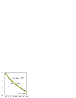
Figure 9: Left: $K$-factor of the stop production cross sections at $Q=m_{\tilde{t}}$ as a function of the stop masses [top/bottom scale]. Right: Production cross sections for the light stop state. The thickness of the NLO curve represents the dependence of the cross sections on the stop mixing angle and the gluino and squark masses. The shaded band indicates the theoretical uncertainty due to the scale dependence [$m/2<Q<2m$].

Figure 10: Normalized transverse-momentum and rapidity distributions for stop production at $Q=m_{\tilde{t}}=200$ GeV.

Figure 11: Left: $K$-factor of the $\tilde{\chi}_{2}^{0}\tilde{\chi}_{2}^{0}$ and $\tilde{\chi}_{1}^{+}\tilde{\chi}_{2}^{0}$ production cross sections at the central scale $Q=m$. Right: Scale dependence of the $\tilde{\chi}_{1}^{+}\tilde{\chi}_{2}^{0}$ cross section. SUGRA parameters: $m_{0}=100$ GeV, $A_{0}=300$ GeV, $\mbox{$\tan\beta$}=4$, $\mu>0$. [The sign convention used in this section differs from the ISAJET convention by a factor of $(-1)$ for $A_{0}$]

Figure 12: The $s$-channel, $(t+u)$-channel and interference contributions to the leading order $\tilde{\chi}_{2}^{0}\tilde{\chi}_{2}^{0}$ and $\tilde{\chi}_{1}^{+}\tilde{\chi}_{2}^{0}$ production cross section. SUGRA parameters as in Fig. 11

Figure 13: The NLO production cross sections included in PROSPINO as a function of the final state particle mass; the arrows indicate the SUGRA inspired scenario: $m_{1/2}=150$ GeV, $m_{0}=100$ GeV, $A_{0}=300$ GeV, $\mbox{$\tan\beta$}=4$, $\mu>0$. All cross sections are given at the average mass scale of the massive final-state particles.

IX Analysis of Next to Leading Order SUSY Production Cross Sections

IX.1 Perturbative QCD Results

The possibility of supersymmetry (SUSY) at the electroweak scale and the ongoing search for the Standard Model (SM) Higgs boson constitute two major related aspects of the motivation for the Tevatron upgrade currently under construction at Fermilab. The increase in the center-of-mass energy to 2 TeV and the luminosity to an expected 2 fb^-1, together with detector improvements, should permit discovery or exclusion of supersymmetric partners of the standard model particles up to much higher masses than at present torah .

Estimates of the production cross sections for pairs of supersymmetric particles may be computed analytically from fixed-order quantum chromodynamics (QCD) perturbation theory. Calculations that include contributions through next-to-leading order (NLO) in QCD have been performed for the production of squarks and gluinos Hopker , top squark pairs Plehn , slepton pairs Baer ; Klasen , gaugino pairs Klasen , and the associated production of gauginos and gluinos BKT . The cross sections can be calculated as functions of the sparticle masses and mixing parameters.

In a recent paper Berger , Berger, Klasen, and Tait provide numerical predictions at next-to-leading order for the production of squark-antisquark, squark-squark, gluino-gluino, squark-gluino, and top squark - antitop squark pairs in proton-antiproton collisions at the hadronic center-of-mass energy 2 TeV. These calculations are based on the analysis of Refs. Hopker ; Plehn , and the CTEQ4M parametrization CTEQ4 of parton densities. The hard scale dependence of the cross section at leading order (LO) in perturbative QCD is reduced at NLO but not absent. An estimate of the theoretical uncertainty at NLO is approximately $\pm 15$ % about a central value. The central value is obtained with the hard scale chosen to be equal to the average of the masses of the produced sparticles, and the band of uncertainty is determined from a variation of the hard scale from half to twice this average mass. The next-to-leading order contributions increase the production cross sections by 50 % and more from their LO values. For example, in the case of squark-antisquark production the next-to-leading order cross section lies above the leading order cross section by 59 %. This increase translates into a shift in the lower limit of the produced squark mass of 19 GeV. The cross sections for squark-antisquark production, gluino pair production, and the associated production of squarks and gluinos of equal mass are of similar magnitude, whereas the squark pair production and top squark-antitop squark production cross sections are smaller by about an order of magnitude Hopker ; Plehn .

The cross sections reported in Ref. Berger are for inclusive yields, integrated over all transverse momenta and rapidities. In the search for supersymmetric states, a selection on transverse momentum will normally be applied in order to improve the signal to background conditions. The theoretical analysis can also be done with similar selections. A tabulation of cross sections for various squark and gluino masses is available upon request from the authors of Ref. Berger .

Next-to-leading order calculations of the production of neutralino pairs, chargino pairs, and neutralino-chargino pairs ar-mon the way to completion Klasen , but final numerical predictions are not yet available for general use.

The strongly interacting squarks and gluinos may also be produced singly in association with charginos and neutralinos. Leading-order production cross sections for the associated production of a chargino plus a squark or gluino and of a neutralino plus a squark or gluino are published assoclo , and a next-to-leading order calculation of associated production of a gaugino plus a gluino is also now published BKT .

Berger, Klasen, and Tait BKT compute total cross sections for all the gaugino-gluino production reactions $\tilde{g}\tilde{\chi}^{0}_{(1-4)}$ and $\tilde{g}\tilde{\chi}^{\rm\pm}_{(1-2)}$ in next-to-leading order SUSY-QCD. For numerical results, they select an illustrative mSUGRA scheme in which the GUT scale common scalar mass $m_{0}=100$ GeV, the common gaugino mass $m_{1/2}=150$ GeV, the trilinear coupling $A_{0}=300$ GeV, $\rm{tan}(\beta)=4$ and $\rm{sgn}(\mu)=+$. (The sign convention for $A_{0}$ is opposite to that in the ISASUGRA code). They convolute the NLO hard partonic cross sections with the CTEQ4M parametrization CTEQ4 of parton densities, and present physical cross sections as a function of the $\tilde{g}$ mass or of the average mass $m=(m_{\tilde{\chi}}+m_{\tilde{g}})/2$. For $p\bar{p}$ collisions at $\sqrt{S}=2$ TeV the cross sections at $m_{\tilde{g}}=300$ GeV range from ${\cal O}(0.2\,{\rm pb})$ for the $\tilde{\chi}^{0}_{2}$ and the $\tilde{\chi}^{\rm\pm}_{1}$ to ${\cal O}(0.2\times 10^{-3}{\rm pb})$ for the $\tilde{\chi}^{0}_{4}$. The $\tilde{g}\tilde{\chi}^{0}_{(1,2)}$ and $\tilde{g}\tilde{\chi}^{\rm\pm}_{1}$ cross sections are of hadronic size despite the fact that the overall coupling strength is ${\cal O}(\alpha_{EW}\alpha_{s})$, not ${\cal O}(\alpha_{s}^{2})$. The masses of the $\tilde{\chi}^{0}_{(1,2)}$ and $\tilde{\chi}^{\rm\pm}_{1}$ ar- significantly smaller in a typical mSUGRA scenario than those of the squarks and gluinos. The phase space and the parton luminosity ar- therefore greater for associated production of a gluino and a gaugino than for a pair of squarks or gluinos, and the smaller coupling strength is compensated. The next-to-leading-order cross sections are enhanced by typically 5% to 15% relative to the leading order values. The theoretical uncertainty resulting from variations of the factorization/renormalization scale is approximately $\pm 10\%$ at NLO for the $\tilde{\chi}^{0}_{2}$ and the $\tilde{\chi}^{\rm\pm}_{1}$, a factor of 2 smaller than the LO variation. Shown in Fig. 14 are the predicted cross sections as a function of $m_{\tilde{g}}$.

Figure 14: Total hadronic cross sections for the associated production of gluinos and gauginos at Run II of the Tevatron. NLO results are shown as solid curves, and LO results as dashed curves. The SUGRA scenario parameter $m_{1/2}$ is varied $\in[100;400]$ GeV, and the cross sections are shown as a function of the physical gluino mass. The chargino cross sections are summed over positive and negative chargino charges.

Baer, Harris, and Reno Baer compute total cross sections for all the slepton pair production reactions $\tilde{e}_{L}\tilde{\nu}_{L}$, $\tilde{e}_{L}\bar{\tilde{e}_{L}}$, $\tilde{e}_{R}\bar{\tilde{e}_{R}}$ and $\tilde{\nu}_{L}\bar{\tilde{\nu}}_{L}$ in next-to-leading order QCD. The analytic calculations are very similar to the QCD corrections to the Standard Model massive lepton-pair production (Drell-Yan) process. Numerical results are based on the CTEQ4M parametrization CTEQ4 of parton densities. For $p\bar{p}$ collisions at $\sqrt{S}=2$ TeV, the cross sections range from ${\cal O}(1{\rm pb})$ at $m_{\rm slepton}=50~{}$GeV to ${\cal O}(10^{-3}{\rm pb})$ at $m_{\rm slepton}=200~{}$GeV. The next-to-leading-order cross sections are enhanced by typically 35% to 40% relative to the leading order values. The theoretical uncertainty resulting from variations in the hard scattering scale and parton distribution functions is approximately $\pm 15\%$. In the mSUGRA model, slepton pair production is most important for small values of the parameter $m_{0}$. The next-to-leading order enhancements of slepton pair cross sections at Tevatron energies can push predictions for leptonic SUSY signals to higher values than typically quoted in the literature in these regions of model parameter space.

For current expectations of the hierarchy of masses and cross sections, consult Ref. torah .

IX.2 Monte Carlo Methods

Experimental searches for supersymmetry rely heavily on Monte Carlo simulations of cross sections and event topologies. Two Monte Carlo generators in common use for hadron-hadron collisions include SUSY processes; they are ISAJET Paige and SPYTHIA Sjostrand ; Mrenna . Both the Monte Carlo approach and the fixed order pQCD approach have different advantages and limitations. Next-to-leading order perturbative calculations depend on very few parameters, e.g., the renormalization and factorization scales, and the dependence of the production cross sections on these parameters is reduced significantly in NLO with respect to LO. Therefore, the normalization of the cross section can be calculated quite reliably if one includes the NLO contributions. On the other hand, the existing next-to-leading order calculations provide predictions only for fully inclusive quantities, e.g., a differential cross section for production of a squark or a gluino, after integration over all other particles and variables in the final state. In addition, they do not include sparticle decays. This approach does not allow for event shape studies nor for experimental selections on missing energy or other variables associated with the produced sparticles or their decay products that are crucial if one wants to enhance the SUSY signal in the face of substantial backgrounds from Standard Model processes.

The natural strength of Monte Carlo simulations consists in the fact that they generate event configurations that resemble those observed in experimental detectors. Through their parton showers, these generators include, in the collinear approximation, contributions from all orders of perturbation theory. In addition, they incorporate phenomenological hadronization models, a simulation of particle decays, the possibility to implement experimental cuts, and event analysis tools. However, the hard-scattering matrix elements in these generators are accurate only to leading order in QCD, and, owing to the rather complex nature of infra-red singularity cancellation in higher orders of perturbation theory, it remains a difficult challenge to incorporate the full structure of NLO contributions successfully in Monte Carlo simulations. The limitation to leading-order hard-scattering matrix elements leads to large uncertainties in the normalization of the cross section. The parton shower and hadronization models rely on tunable parameters, another source of uncertainties.

In Ref. Berger a method is suggested to improve the accuracy of the normalization of cross sections computed through Monte Carlo simulations. In this approach, the renormalization and factorization (hard) scale in the Monte Carlo LO calculation is chosen in such a way that the normalization of the Monte Carlo LO calculation agrees with that of the NLO perturbative calculation. The scale choice depends on which partonic subprocess one is considering and on the kinematics. This choice of the hard scale will affect both the hard matrix element and the initial-state and final-state parton shower radiation. On the other hand, an alternative rescaling of the cross section by an overall $K$-factor will have no bearing on the parton shower radiation. A reduction in the hard scale leads generally to less evolution and less QCD radiation, and vice-versa, in the initial- and final-state showering. A change of the hard scale will be reflected in the normalization of the cross section as well as in the event shape. Investigations are underway to determine how significant the changes are in computed final state momentum distributions.

X Sparticle Cross Sections and Branching Fractions

X.1 Sparticle production cross sections

If the mSUGRA model is correct, then there may be a wide variety of new sparticles that can be produced at the Tevatron collider. What is especially important for determining the signal events is the relative sparticle production rates at different points in model parameter space. A simplifying feature of the mSUGRA model is that the gaugino mass unification condition is approximately true throughout parameter space:

$${M_{1}\over\alpha_{1}}={M_{2}\over\alpha_{2}}={M_{3}\over\alpha_{3}}\,,$$ (157)

where $\alpha_{1}={5\over 3}{g^{\prime 2}\over 4\pi}$ and $g^{\prime}$ is the Standard Model U(1) gauge coupling. In particular, this relation holds at the weak scale, so that if we know any of the weak scale gaugino masses $M_{i}$, then we can calculate the others.

Another simplifying feature of mSUGRA models derived from the radiative electroweak symmetry breaking (REWSB) constraint is that over most of parameter space, the magnitude of the $\mu$ parameter

$$|\mu|\gg M_{1},\ M_{2},$$ (158)

so that the two lightest neutralinos and lightest chargino are gaugino-like and the two heaviest neutralinos and heavier chargino are higgsino-like. The exception to this statement occurs at parameter space values near the regions where the REWSB mechanism almost breaks down, and at large $\tan\beta$; in both of these regions, $|\mu|$ can become quite small.

Given the above inputs, it is possible to plot typical sparticle pair production cross sections expected at the Tevatron colliderprod . In Fig. 17, we plotbh-bckt sparticle cross sections as a function of $m_{\tilde{g}}$ assuming five generations of degenerate squark masses, for a) $m_{\tilde{q}}=m_{\tilde{g}}$ and b) $m_{\tilde{q}}=2m_{\tilde{g}}$, assuming $\mu=+m_{\tilde{g}}$, and $\tan\beta=3$. In this plot, $m_{\tilde{g}}$ is the pole gluino mass. The region to the left of the vertical line is excluded by the LEP2 chargino mass limit $m_{\widetilde{\chi}^{\pm}_{1}}>90$ GeV. Thus, it can be seen that direct chargino pair production $\widetilde{\chi}^{\pm}_{1}\widetilde{\chi}^{\pm}_{1}$ and $\widetilde{\chi}^{\pm}_{1}\widetilde{\chi}^{0}_{2}$ production dominate over the strongly produced $\tilde{g}\tilde{g}$, $\tilde{g}\tilde{q}$ and $\tilde{q}\tilde{q}$ cross sections over essentially all of parameter space for which $|\mu|\gg M_{1},\ M_{2}$. The reaction $\widetilde{\chi}^{\pm}_{1}\widetilde{\chi}^{0}_{1}$ is also sub-dominant, while the squark or gluino plus chargino or neutralino associated production reactions (summed over all sparticle types and labelled by dash-dot-dot curves) are also relatively suppressed. These qualitative features hold for both frames shown.

Figure 15: Sparticle production cross sections as a function of $m_{\tilde{g}}$ for $\mu=+m_{\tilde{g}}$ and $\tan\beta=3$.

Figure 16: Sparticle production cross sections as a function of $m_{\tilde{g}}$ for $\mu=-m_{\tilde{g}}$ and $\tan\beta=3$.

Figure 17: a) Slepton production cross sections at NLO as a function of $m_{\tilde{\ell}}$; b) the ratio ${\sigma_{NLO}/\sigma_{LO}}$ as a function of $m_{\tilde{\ell}}$.

Similar results are shown in Fig. 17 for $\mu=-m_{\tilde{g}}$. In this case, for low values of $m_{\tilde{g}}$ with $m_{\tilde{q}}\simeq m_{\tilde{g}}$, the strong production cross sections can be dominant, but only in parameter space regions now already excluded by LEP2.

The implications of these results are that in the mSUGRA model, $\widetilde{\chi}^{\pm}_{1}\widetilde{\chi}^{\pm}_{1}$ and $\widetilde{\chi}^{\pm}_{1}\widetilde{\chi}^{0}_{2}$ will likely be the dominant production cross sections over much of parameter space, and their signals may well lead to the maximal reach of Tevatron experiments for SUSY particles. For instance, the $\widetilde{\chi}^{\pm}_{1}\widetilde{\chi}^{0}_{2}\rightarrow 3\ell+\not\!\!{E_{T}}$ signal can yield a Run 2 reach of Tevatron experiments to values of $m_{\tilde{g}}\simeq 600$ GeVbcpt .

If the parameter $m_{0}$ is very small, then slepton and sneutrino masses may be relatively small and their production cross sections may be important. These cross sections are shown at next-to-leading orderbhr in Fig. 17a), while the ratio ${\sigma_{NLO}/\sigma_{LO}}$ is shown in Fig. 17b).

X.2 Sparticle branching fractions

Once sparticles are produced, they typically decay through a cascade of decays with lighter sparticles until it terminates with the production of the lightest SUSY particle, usually assumed to be absolutely stable. Sparticle branching fractions are in general complicated functions of SUSY model parameter spacedecay . These branching fractions are embedded in several event generator programs (such as ISAJETbh-isajet ) and PYTHIAbh-pythia ), and separate programs exist that can output complete lists of sparticle branching fractions. From the previous section, however, it is clear that $\widetilde{\chi}^{\pm}_{1}$ and $\widetilde{\chi}^{0}_{2}$ production cross sections are dominant, so their branching fractions will be the most relevant for SUSY searches at the Tevatron within the mSUGRA framework.

If the parameter $m_{1/2}$ is small, then the light chargino $\widetilde{\chi}^{\pm}_{1}$ usually decays via a 3-body mode via virtual $W$, $\tilde{q}_{L}$, $\tilde{\ell}_{L}$ or $H^{\pm}$ exchange. Over much of paramater space, the $W^{*}$ exchange dominates, so that the $\widetilde{\chi}^{\pm}_{1}\rightarrow\widetilde{\chi}^{0}_{1}f\bar{f^{\prime}}$ branching fraction is similar to the $W\rightarrow f\bar{f^{\prime}}$ one. Exceptions can occur if $m_{0}$ is very small, in which case light virtual sleptons can enhance the leptonic decays, or if $\tan\beta$ is large so that large $\tau$ Yukawa coupling effects enhance decays to $\tau$ leptonsbcdpt . If $m_{1/2}$ becomes large, then ultimately $\widetilde{\chi}^{\pm}_{1}$ becomes so heavy that the decays $\widetilde{\chi}^{\pm}_{1}\rightarrow\widetilde{\chi}^{0}_{1}W$ (or even decays to sfermions) become accessible.

If $m_{1/2}$ is small, then the neutralino $\widetilde{\chi}^{0}_{2}$ can decay via 3-body modes $\widetilde{\chi}^{0}_{2}\rightarrow\widetilde{\chi}^{0}_{1}f\bar{f}$ where $f=\ell,\ \nu$ or $q$’s. These relative branching fractions are very model dependent. For instance, for moderate $m_{0}$ and $\mu<0$, the $\widetilde{\chi}^{0}_{2}$ leptonic decays are enhanced, yielding a large Tevatron reach for SUSY via $\widetilde{\chi}^{0}_{2}\rightarrow\widetilde{\chi}^{0}_{1}\ell\bar{\ell}$bh-bckt ; bcpt . However, for the opposite sign of $\mu$, the leptonic decays can be suppressed, and there is no reach for $3\ell$ events by the Tevatron beyond the parameter space limits established by LEP2bh-bckt ; bcpt . As $m_{1/2}$ increases, the decays $\widetilde{\chi}^{0}_{2}\rightarrow\widetilde{\chi}^{0}_{1}h$ or $\widetilde{\chi}^{0}_{2}\rightarrow\widetilde{\chi}^{0}_{1}Z$ can open up; the former decay is known as a “spoiler mode”, since when it opens it can dominate the branching fractions and destroy the clean $3\ell$ signal from $\widetilde{\chi}^{\pm}_{1}\widetilde{\chi}^{0}_{2}$ production. If $m_{0}$ becomes small, then $\widetilde{\chi}^{0}_{2}$ might be able to decay to real or virtual sleptons and/or sneutrinos, and leptonic decays are again enhanced. As $\tan\beta$ becomes large, $b$-quark and $\tau$-lepton Yukawa couplings can become important, and if $m_{0}$ is low enough, decays to 3rd generation fermions can be enhanced. The decay rate of $\widetilde{\chi}^{\pm}_{1}$ and $\widetilde{\chi}^{0}_{2}$ to various fermions and sfermions versus $\tan\beta$ is shown in Fig. 18 for small and large values of $m_{0}$. In these plots, the enhancement of decays to third generation fermions for low $m_{0}$ is evident.

Figure 18: Chargino ($\widetilde{\chi}^{\pm}$) and neutralino ($\widetilde{\chi}^{0}$) branching fractions versus $\tan\beta$. In a) and b), we take the parameters ($m_{0},m_{1/2},A_{0})=(150,150,0)$ GeV while in c) and d) we take ($m_{0},m_{1/2},A_{0})=(150,500,0)$ GeV. In all frames, $\mu>0$ and $m_{t}=170$ GeV. The discontinuities are an artifact of the narrow width approximation. In ISAJET, widths for three body and two body decays are separately computed: the transition is, of course, smooth since the virtual particle smoothly goes on-shell.

XI LEP Constraints on mSUGRA

Searches for supersymmetry in $e^{+}e^{-}$ collisions at LEP have already probed significant regions of the mSUGRA parameter space. Recent runs at 133, 161, 172, 183 and 189 GeV center-of-mass energy have excluded much of the region at low gaugino mass, and future runs at $\sim 192-200{\rm\,Ge\kern-1.25ptV}$ will further extend the experimentally forbidden region, or discover supersymmetry. In this section we summarize those of the LEP bounds which most strongly constrain the mSUGRA parameter space. It includes bounds from the run at 183 GeV centre-of-mass energy, and preliminary results from the run at 189 GeV can be found on the web pages for the individual LEP experiments urls and from the LEP-SUSY Working Group home page lepsusywg .

Supersymmetric particle searches at LEP include searches for charginos and neutralinosalcn183 ; decn183 ; l3cn183 ; opcn183 , sleptonsalsl183 ; desl183 ; l3sl183 ; opsl183 , stops and sbottomsdesl183 ; tb183 , and Higgs bosons. Constraints from the Higgs searches will be discussed in detail in another section. The combined constraints are presented as exclusion plots in the $\{m_{1\!/2},m_{0}\}$ plane, at fixed $\tan\beta$ and $A_{0}$. The outer envelope of the excluded regions in mSUGRA is generally set by the chargino and slepton searches alone, though for large $A_{0}$ the stop bounds can become important as well, as the lighter stop mass squared can be driven negative at large $A_{0}$. The stop mass constraints will be summarized later in this secton.

Chargino pairs are produced via s-channel photon or $Z^{0}$ exchange and t-channel sneutrino exchange. In most of the mSUGRA parameters space, the chargino production rate is large enough, and the chargino-neutralino mass difference sufficient, so that the chargino mass bound effectively saturates the kinematic limit. However, destructive interference between the sneutrino and gauge boson exchange channels can reduce the bounds for sneutrino masses slightly above the chargino mass. For sneutrino masses just below the chargino mass, the produced charginos can decay into a sneutrino and soft lepton, and if the mass difference between the sneutrino and chargino is sufficiently small, the soft leptons will remain undetected.

Fortunately, much of the latter loophole is covered by the selectron searches. Slepton pairs of all generations are produced via s-channel photon or $Z^{0}$ exchange and t-channel neutralino exchange (for selectrons). However, limits on smuon and stau production do not significantly strengthen the bounds obtained from selectron searches alone. Fig. 19 and Fig. 20 display the combined selectron and chargino bounds alcn in the $\{m_{1\!/2},m_{0}\}$ plane for $\tan\beta=2,3,10$, and 35, for $\mu<0$ and $\mu>0$. Here $A_{0}=0$, but the constraints are too not sensitive to $A_{0}$. The chargino bound is strongest at large $m_{0}$, where the sneutrino mass is large. As $m_{0}$ is decreased, the chargino constraint is observed to become weaker as destructive interference between the s-channel and t-channel processes becomes important, and near $m_{0}\sim 50-75{\rm\,Ge\kern-1.25ptV}$ the sneutrino mass drops below the chargino mass, and the chargino bound retreats. For $\mu>0$, the discontinuity in the chargino bound is covered completely by the slepton bound. The bounds in Figs. 19 and 20 are computed neglecting stau mixing. Stau mixing changes the overlap between the regions which yield a kinematically accessible stau and those giving a light selectron, and at large $\tan\beta$ it can open up small gaps in the chargino bounds, where the stau-neutralino mass difference is small ($<5$ GeV) susywg , and where the chargino can decay invisibly via chargino $\rightarrow$ stau + neutrino followed by stau $\rightarrow$ neutralino + tau. At low $\tan\beta$ these configurations are covered by selectron searches.

For sufficiently large $A_{0}$, the mass of the lighter stop tends to be driven negative, so separate bounds on the mass of the lightest stop can provide important constraints in this region. The dominant constraints come from searches for $\tilde{t}\rightarrow c\tilde{\chi}^{0}$ and $\tilde{t}\rightarrow bl\tilde{\nu}$ tb183 , and the corresponding limits are displayed in Fig.21. Bounds on the stop mass depend on both the stop-neutralino (or stop-sneutrino) mass difference and on the mixing angle between left and right stops. However, unless the mass of the stop is less than $10{\rm\,Ge\kern-1.25ptV}$ above both the mass of the neutralino and sneutrino, an absolute lower bound of $74{\rm\,Ge\kern-1.25ptV}$ on the mass of the lightest stop can be obtained tb183 , independent of the stop mixing angle. Since the stop mixing angle is fixed as a function of the mSUGRA parameters, this bound may be improved by a few ${\rm\,Ge\kern-1.25ptV}$ in any specific case.

In the general MSSM, searches for associated neutralino $\tilde{\chi}^{0}_{1}\tilde{\chi}^{0}_{2}$ production through s-channel $Z^{0}$ or t-channel selectron exchange can play a rôle in limiting the parameter space. Fig. 22 displays the region of $\{\mu,M_{2}\}$ parameter space excluded by the combined set of LEP MSSM constraints opcn183 for two representative values of $\tan\beta$, taking a common mass parameter $m_{0}$ for the sfermions. One can also extract from the combined constraints a lower bound on the neutralino mass as a function of $\tan\beta$, and this is displayed for the MSSM opcn183 in Fig. 23.

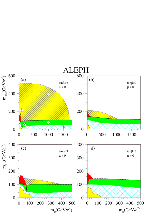
Figure 19: Combined chargino and selectron bounds from LEP 183, for $\tan\beta=2$ and 3, and for $A_{0}=0$. Region 1 is theoretically forbidden. The other regions are excluded by the $Z$ width measurement at LEP1 (2), chargino (3) and slepton (4) searches, and by Higgs boson searches (5). The dashed lines represent the kinematic limit for direct chargino searches.

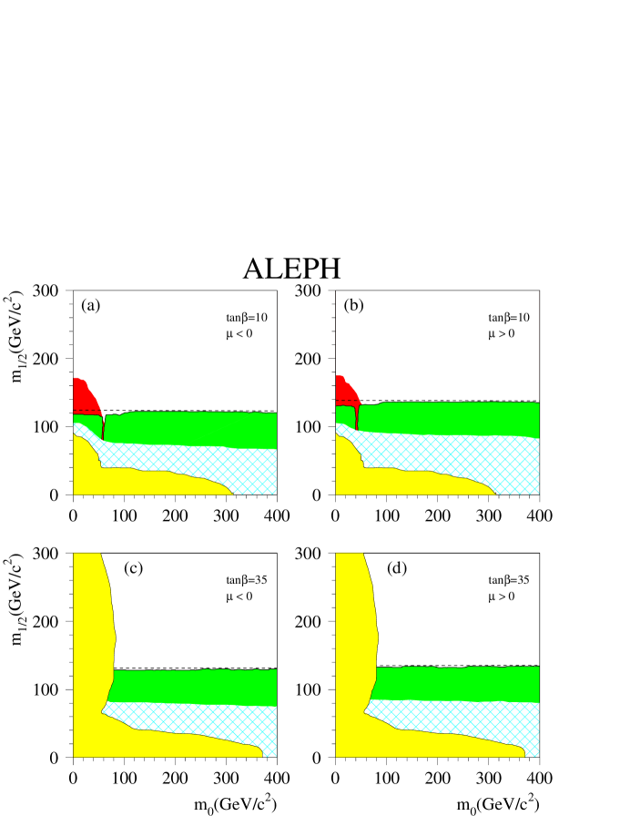
Figure 20: Combined chargino and selectron bounds from LEP 183, for $\tan\beta=10$ and 35, and for $A_{0}$. The regions are defined as in Fig. 19

   

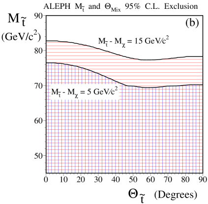
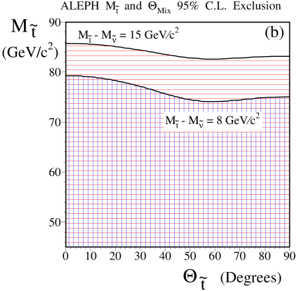
Figure 21: Lower bound on the stop mass as a function of $\tan\beta$, for a) $\tilde{t}\rightarrow c\tilde{\chi}^{0}$ and b) $\tilde{t}\rightarrow bl\tilde{\nu}$.

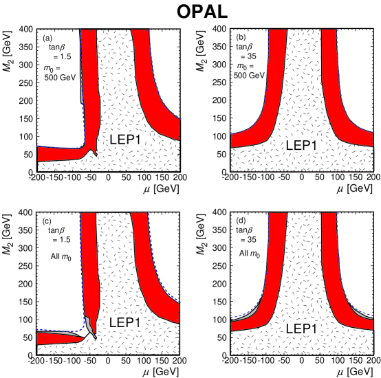
Figure 22: Exclusion regions at 95% C.L. in the ($M_{2}$,$\mu$) plane with $m_{0}\geq 500$ GeV for (a) $\tan\beta=1.5$ and for (b) $\tan\beta=35$. Exclusion regions valid for all $m_{0}$ for (c) $\tan\beta=1.5$ and for (d) $\tan\beta=35$. The speckled areas show the LEP1 excluded regions and the dark shaded areas show the additional exclusion region using the data from $\sqrt{s}=181$–184 GeV. The kinematical boundaries for $\tilde{\chi}^{+}_{1}\tilde{\chi}^{-}_{1}$ production are shown by the dashed curves. The light shaded region in (a) extending beyond the kinematical boundary of the $\tilde{\chi}^{+}_{1}\tilde{\chi}^{-}_{1}$ production is obtained due to the interpretation of the results from the direct neutralino searches. The light shaded regions elsewhere show the additional exclusion regions due to direct neutralino searches and other OPAL search results (see opcn183 ).

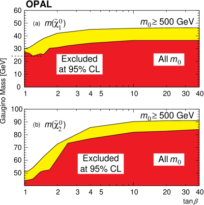
Figure 23: The 95% C.L. mass limit on (a) the lightest neutralino $\tilde{\chi}^{0}_{1}$ and (b) the second-lightest neutralino $\tilde{\chi}^{0}_{2}$ as a function of $\tan\beta$ for $m_{0}\geq 500$ GeV. The mass limit on $\tilde{\chi}^{0}_{2}$ is for the additional requirement of $m_{\tilde{\chi}^{0}_{2}}-m_{\tilde{\chi}^{0}_{1}}>10$ GeV. The exclusion region for $m_{0}\geq 500$ GeV is shown by the light shaded area and the excluded region valid for all $m_{0}$ values by the dark shaded area.

XII SUGRA Limits in Run I

XII.1 Introduction

There has been a great effort in searches for SUSY particles by CDF and DØ using data samples in $p\overline{p}$ collisions at $\sqrt{s}$ = 1.8 TeV at the Fermilab Tevatron. The data were collected during the 1992-93 (Run Ia) and 1994-95 (Run Ib) runs.

With the assumption of the gaugino unification provided by supergravity (SUGRA) basicSUGRA , the Minimal Supersymmetric Standard Model (MSSM) framework SUSYreview has a simple mass relation between gluino ($\tilde{g}$), chargino ($\tilde{\chi}_{1}^{\pm}$) and neutralinos ($\tilde{\chi}_{2}^{0}$ and $\tilde{\chi}_{1}^{0}$): $(1/3\sim 1/4)\;M(\mbox{$\tilde{g}$})\approx M(\mbox{$\tilde{\chi}_{1}^{\pm}$})\approx M(\mbox{$\tilde{\chi}_{2}^{0}$})\approx 2~{}M(\mbox{$\tilde{\chi}_{1}^{0}$})$. We assume the lightest neutralino ($\tilde{\chi}_{1}^{0}$) is the lightest supersymmetric particle (LSP) and stable. The LSPs do not interact with the detector and therefore result in missing transverse energy (${E\!\!\!\!/_{T}}$).

One canonical SUSY signature is trilepton events, which would come from chargino-neutralino ($\tilde{\chi}_{1}^{\pm}$$\tilde{\chi}_{2}^{0}$) pair production with subsequent leptonic decays ($\mbox{$\tilde{\chi}_{1}^{\pm}$}\rightarrow\ell^{\pm}\nu\mbox{$\tilde{\chi}_{1}^{0}$}$ and $\mbox{$\tilde{\chi}_{2}^{0}$}\rightarrow\mbox{$\ell^{+}\ell^{-}$}\mbox{$\tilde{\chi}_{1}^{0}$}$) susy_trilepton . Another signature is squark and gluino ($\tilde{q}$ and $\tilde{g}$) production followed by decays into the LSP and jets. Yet another is based on the Majorana nature of the gluino, which allows the gluino to decay into a chargino of either sign. One consequently searches for like-sign (LS) dilepton pairs from cases where a pair of gluinos have decayed into charginos of the same sign susy_dilepton .

Table 4 shows decay branching ratios of chargino, neutralino, gluino, and squarks, for four minimal SUGRA (mSUGRA) cases: (1) $M(\mbox{$\tilde{q}$})\gg M(\mbox{$\tilde{g}$})$; (2) $M(\mbox{$\tilde{q}$})\simeq M(\mbox{$\tilde{g}$})+7\ \mbox{$\;{\rm GeV}/c^{2}$}$; (3) $M(\mbox{$\tilde{q}$})\simeq M(\mbox{$\tilde{g}$})-7\ \mbox{$\;{\rm GeV}/c^{2}$}$; (4) $M(\mbox{$\tilde{q}$})/M(\mbox{$\tilde{g}$})\simeq 0.9$. Other mSUGRA parameters are fixed as $\tan\beta=2$, $\mu<0$ and $A_{0}=0$. These mSUGRA points can be characterized as:

• The gluino pair production is dominant, and the decays of $\tilde{\chi}_{1}^{\pm}$ and $\tilde{\chi}_{2}^{0}$ are key. For example, $Br(\mbox{$\tilde{g}$}\rightarrow e^{\pm}+X)$ = 4.9% and $Br(\mbox{$\tilde{g}$}\rightarrow e^{+}e^{-}+X)$ = 2.6%. We should access to this point via trilepton, $\mbox{${E\!\!\!\!/_{T}}$}+jets$, and LS dilepton + $\mbox{${E\!\!\!\!/_{T}}$}+jets$ channels.

• The $\tilde{g}\tilde{g}$, $\tilde{q}$$\bar{\tilde{q}}$ and $\tilde{g}\tilde{q}$ production is dominant. The key decay is $\mbox{$\tilde{g}$}\rightarrow\mbox{$\tilde{b}$}b$, because $M(\mbox{$\tilde{b}$})-M(\mbox{$\tilde{g}$})>M(b)$ and $M(\mbox{$\tilde{b}$})<M(\mbox{$\tilde{q}$})$. We have $Br(\mbox{$\tilde{g}$}\rightarrow e^{\pm}+X)$ = 0.6% and $Br(\mbox{$\tilde{g}$}\rightarrow e^{+}e^{-}+X)$ = 17.2%. Leptons are also expected from light squark decays. We should access to this point via trilepton, $\mbox{${E\!\!\!\!/_{T}}$}+jets$, and $2\ell+\mbox{${E\!\!\!\!/_{T}}$}+jets$ channels.

• Similar to Case 2. $Br(\mbox{$\tilde{g}$}\rightarrow e^{\pm}+X)$ = 0.7% and $Br(\mbox{$\tilde{g}$}\rightarrow e^{+}e^{-}+X)$ = 16.5%. This point is close to DØ’s 95% C.L. exclusion contour based on $\mbox{${E\!\!\!\!/_{T}}$}+$ jets and $ee+\mbox{${E\!\!\!\!/_{T}}$}+$ jets analyses (see Section XII.4.2).

• $\mbox{$\tilde{\chi}_{2}^{0}$}\rightarrow\mbox{$e^{+}e^{-}$}\mbox{$\tilde{\chi}_{1}^{0}$}$ is suppressed, because $\mbox{$\tilde{\nu}$}_{L}$ (43 $\;{\rm GeV}/c^{2}$) is lighter than $\tilde{e}_{R}$ (49 $\;{\rm GeV}/c^{2}$) and $\tilde{e}_{L}$ (75 $\;{\rm GeV}/c^{2}$). The electron from $\mbox{$\tilde{e}_{R}$}\rightarrow e\mbox{$\tilde{\chi}_{1}^{0}$}$ ($Br=100\%$) will be softer, so that the LS dilepton + ${E\!\!\!\!/_{T}}$ channel will be important for a search for a direct production of $\tilde{\chi}_{1}^{\pm}$$\tilde{\chi}_{2}^{0}$. Note $Br(\mbox{$\tilde{g}$}\rightarrow e^{\pm}+X)$ = 6.3% and $Br(\mbox{$\tilde{g}$}\rightarrow e^{+}e^{-}+X)$ = 0.7%.

Given the large mass for the top quark, Yukawa interactions should drive one of the top squark (stop) masses to a value much lower than that of the other squarks. There are three alternative decay modes possible for the lighter stop ($\tilde{t}_{1}$) if it is lighter than the top quark lstop : (i) $\mbox{$\tilde{t}_{1}$}\rightarrow c\ \mbox{$\tilde{\chi}_{1}^{0}$}$ if the charginos, sleptons, sneutrinos are heavier than the stop; or (ii) $\mbox{$\tilde{t}_{1}$}\rightarrow b\ \mbox{$\tilde{\chi}_{1}^{\pm}$}$ if the chargino is lighter than the stop; or (iii) $\mbox{$\tilde{t}_{1}$}\rightarrow\ell\mbox{$\tilde{\nu}$}b\;(\mbox{$\tilde{\ell}$}\nu b)$ if sneutrinos (or sleptons) are light enough.

The effect of the Yukawa interactions on the bottom squark (sbottom) is much smaller, because the bottom quark mass is much smaller than the top quark mass. A large splitting between mass eigenstates can still occur when the values of $\tan\beta$ are large. Thus, one of the sbottoms ($\tilde{b}_{1}$) can be lighter than other squarks. We could study a direct production of sbottom pair ($\mbox{$p\overline{p}$}\rightarrow\mbox{$\tilde{b}_{1}$}\mbox{$\bar{\tilde{b}}_{1}$}+X$) and an indirect production via $\mbox{$\tilde{g}$}\rightarrow\bar{b}\ \mbox{$\tilde{b}_{1}$}$. The decay modes could be (i) $\mbox{$\tilde{b}_{1}$}\rightarrow b\ \mbox{$\tilde{\chi}_{1}^{0}$}$ and (ii) $\mbox{$\tilde{b}_{1}$}\rightarrow b\ \mbox{$\tilde{\chi}_{2}^{0}$}$ lsbot .

We summarize the current results of searches for SUSY particles in the MSSM or SUGRA frameworks from CDF and DØ experiments using the data taken in 1992-95 (Run Ia+Ib; corresponding to approximately 110 $\;{\rm pb}^{-1}$). It should be noted that results based on the data in 1992-93 (Run Ia; 20 $\;{\rm pb}^{-1}$) can be found in elsewhere RIPS and are not covered in this paper.

Table 4: Example of decay branching ratios of chargino, neutralino, gluino, and squarks for four reference points in the mSUGRA model (isajet version 7.20): (1) $M(\mbox{$\tilde{q}$})\gg M(\mbox{$\tilde{g}$})$; (2) $M(\mbox{$\tilde{q}$})\simeq M(\mbox{$\tilde{g}$})+7\ \mbox{$\;{\rm GeV}/c^{2}$}$; (3) $M(\mbox{$\tilde{q}$})\simeq M(\mbox{$\tilde{g}$})-7\ \mbox{$\;{\rm GeV}/c^{2}$}$; (4) $M(\mbox{$\tilde{q}$})/M(\mbox{$\tilde{g}$})\simeq 0.9$. Here $m_{0}$ ($m_{1/2}$) is a common scalar (gaugino) mass. Other mSUGRA parameters are fixed as $\tan\beta=2$, $\mu<0$ and $A_{0}=0$.

mSUGRA: $(m_{0},m_{1/2})\rightarrow$	(500, 90)	(170, 90)	(140, 90)	(  0, 90)
Mass ($\;{\rm GeV}/c^{2}$)
$\tilde{\chi}_{1}^{\pm}$/$\tilde{\chi}_{2}^{0}$	85.1/85.5	89.2/89.9	89.5/90.1	90.0/90.1
$\tilde{\chi}_{1}^{0}$	39.7	40.4	40.4	40.6
$\tilde{g}$	292	275	273	264
$\tilde{q}$	543	283	267	231
$\mbox{$\tilde{b}$}_{1}$/$\mbox{$\tilde{b}$}_{2}$	426/541	251/281	242/264	219/227
$\tilde{t}_{1}$/$\tilde{t}_{2}$	297/458	247/309	241/304	225/296
Decay Branching Ratio (%)
$\mbox{$\tilde{\chi}_{1}^{+}$}\rightarrow\mbox{$\tilde{\chi}_{1}^{0}$}e^{+}\nu_{e}$	11.0	11.5	12.3	27.8 ($\mbox{$\tilde{\nu}$}e$)
$\mbox{$\tilde{\chi}_{2}^{0}$}\rightarrow\mbox{$\tilde{\chi}_{1}^{0}$}e^{+}e^{-}$	6.4	19.1	21.3	3.8 ($\tilde{e}e$)
$\mbox{$\tilde{g}$}\rightarrow\mbox{$\tilde{\chi}_{2}^{0}$}q\bar{q},\;\mbox{$\tilde{\chi}_{2}^{0}$}\mbox{$b\overline{b}$}$	41.3	0.0	0.0	0.0
$\mbox{$\tilde{g}$}\rightarrow\mbox{$\tilde{\chi}_{1}^{+}$}\bar{u}d,\;\mbox{$\tilde{\chi}_{1}^{+}$}\bar{c}s,\;+c.c.$	44.9	5.6	0.0	0.0
$\mbox{$\tilde{g}$}\rightarrow\mbox{$\tilde{q}$}\bar{q}$	0.0	0.0	17.3	70.7
$\mbox{$\tilde{g}$}\rightarrow\mbox{$\tilde{b}$}_{1}b$	0.0	90.0	77.5	18.4
$\mbox{$\tilde{g}$}\rightarrow\mbox{$\tilde{b}$}_{2}b$	0.0	0.0	5.2	10.9
$\tilde{u}_{L}\rightarrow\mbox{$\tilde{\chi}_{2}^{0}$}u$	7.1	27.1	27.3	25.7
$\tilde{u}_{L}\rightarrow\mbox{$\tilde{\chi}_{1}^{+}$}d$	15.3	65.0	66.8	67.2
$\tilde{u}_{L}\rightarrow\mbox{$\tilde{g}$}\ u$	76.9	2.5	0.0	0.0
$\tilde{d}_{L}\rightarrow\mbox{$\tilde{\chi}_{2}^{0}$}d$	7.7	33.9	34.9	35.1
$\tilde{d}_{L}\rightarrow\mbox{$\tilde{\chi}_{1}^{-}$}u$	14.8	61.9	63.3	62.1
$\tilde{d}_{L}\rightarrow\mbox{$\tilde{g}$}\ d$	77.3	2.8	0.0	0.0
$\tilde{u}_{R}\rightarrow\mbox{$\tilde{\chi}_{2}^{0}$}u$	0.0	1.6	1.8	1.6
$\tilde{u}_{R}\rightarrow\mbox{$\tilde{g}$}\ u$	94.8	11.1	0.0	0.0
$\tilde{d}_{R}\rightarrow\mbox{$\tilde{\chi}_{2}^{0}$}d$	0.0	1.1	1.8	1.6
$\tilde{d}_{R}\rightarrow\mbox{$\tilde{g}$}\ d$	98.6	33.3	0.0	0.0
$\tilde{b}_{1}\rightarrow\mbox{$\tilde{\chi}_{2}^{0}$}b$	12.6	99.8	99.7	98.4
$\tilde{b}_{1}\rightarrow\mbox{$\tilde{\chi}_{1}^{-}$}t$	16.0	0.0	0.0	0.0
$\tilde{b}_{1}\rightarrow\mbox{$\tilde{g}$}\ b$	71.2	0.0	0.0	0.0
$\tilde{b}_{2}\rightarrow\mbox{$\tilde{\chi}_{2}^{0}$}b$	0.0	1.7	1.7	1.6
$\tilde{b}_{2}\rightarrow\mbox{$\tilde{g}$}\ b$	98.6	2.5	0.0	0.0
$\tilde{t}_{1}\rightarrow\mbox{$\tilde{\chi}_{1}^{0}$}t$	79.5	25.5	16.7	6.1
$\tilde{t}_{1}\rightarrow\mbox{$\tilde{\chi}_{2}^{0}$}t$	6.2	0.0	0.0	6.8
$\tilde{t}_{1}\rightarrow\mbox{$\tilde{\chi}_{1}^{+}$}b$	14.3	74.5	74.5	55.3

XII.2 CDF and DØ Detectors

XII.2.1 CDF

The CDF detector is a general purpose detector described in detail elsewhere cdf1det ; cdftop94 . The inner most part of CDF, the silicon vertex detector (SVX^′), allows a precise measurement of a track’s impact parameter with respect to the primary vertex in the plane transverse to the beam direction. The position of the primary vertex along the beam direction is determined by a time projection chamber. The momenta of the charged particles are measured in the central drift chamber which is located inside a 1.4 T superconducting solenoidal magnet. Outside the drift chamber there is a calorimeter, which is organized into electromagnetic and hadronic components, with projective towers covering the pseudo-rapidity range $|\eta|<4.2$. The muon system is located outside the calorimeter and covers the range $|\eta|<1.0$.

XII.2.2 DØ

The DØ detector is a large multipurpose detector used to measure charged leptons, photons, and jets. The hermeticity of the detector allows for a good measurement of the missing transverse energy. Moving radially from the beamline the DØ detector consists of a non-magnetic central tracking system, a compact uranium/liquid-argon sampling calorimeter, and a muon spectrometer d01det .

XII.3 Search for $\tilde{\chi}_{1}^{\pm}$$\tilde{\chi}_{2}^{0}$ Using Trilepton Events

It has long been suggested that one of the most promising channels for the discovery of SUSY at a hadron collider is three isolated charged leptons plus missing energy, arising from $\tilde{\chi}_{1}^{\pm}$$\tilde{\chi}_{2}^{0}$ pair production with subsequent leptonic decays ($\mbox{$\tilde{\chi}_{1}^{\pm}$}\rightarrow\ell\nu\mbox{$\tilde{\chi}_{1}^{0}$}$ and $\mbox{$\tilde{\chi}_{2}^{0}$}\rightarrow\ell^{+}\ell^{-}\mbox{$\tilde{\chi}_{1}^{0}$}$) susy_trilepton .

DØ and CDF search for direct production of $\tilde{\chi}_{1}^{\pm}$$\tilde{\chi}_{2}^{0}$ in the trilepton channels ($e^{+}e^{-}e$, $e^{+}e^{-}\mu$, $e\mu^{+}\mu^{-}$ and $\mu^{+}\mu^{-}\mu$). The detailed analyses of the DØ and CDF searches are described elsewhere d0_tril ; cdf_tril . Table 5 is a summary of the trilepton selections at DØ and CDF. It should be noted that the $p_{T}$ cuts in the DØ analysis depend on the triggers used, so that we only indicate approximate values. Both analyses find no events in their selection cuts, which are consistent with expectation from SM background events.

Table 5: Summary of DØ and CDF trilepton analyses in Run I. The $p_{T}$ cuts in the DØ analysis depend on the trilepton channel ($eee$, $ee\mu$, $e\mu\mu$ or $\mu\mu\mu$). ${E\!\!\!\!/_{T}}$, $p_{T}$, and $M$ are given in GeV, $\;{\rm GeV}/c$, and $\;{\rm GeV}/c^{2}$, respectively. Experimentally, electrons (muons) are selected by $E_{T}$ ($p_{T}$). We simply refer $p_{T}$ for both electron and muon.

Experiment	DØ d0_tril	CDF cdf_tril
${\int{\cal L}\;dt}$	107 $\;{\rm pb}^{-1}$	106 $\;{\rm pb}^{-1}$
Primary cuts:
$p_{T}$ for $\ell_{1}$, $\ell_{2}$, $\ell_{3}$	${\mathrel{\mathchoice{\lower 4.0pt\vbox{\halign{$\mathsurround=0pt\displaystyle\hfil#\hfil$\cr>\crcr\sim\crcr}}}{\lower 4.0pt\vbox{\halign{$\mathsurround=0pt\textstyle\hfil#\hfil$\cr>\crcr\sim\crcr}}}{\lower 4.0pt\vbox{\halign{$\mathsurround=0pt\scriptstyle\hfil#\hfil$\cr>\crcr\sim\crcr}}}{\lower 4.0pt\vbox{\halign{$\mathsurround=0pt\scriptscriptstyle\hfil#\hfil$\cr>\crcr\sim\crcr}}}}}\ 10$, ${\mathrel{\mathchoice{\lower 4.0pt\vbox{\halign{$\mathsurround=0pt\displaystyle\hfil#\hfil$\cr>\crcr\sim\crcr}}}{\lower 4.0pt\vbox{\halign{$\mathsurround=0pt\textstyle\hfil#\hfil$\cr>\crcr\sim\crcr}}}{\lower 4.0pt\vbox{\halign{$\mathsurround=0pt\scriptstyle\hfil#\hfil$\cr>\crcr\sim\crcr}}}{\lower 4.0pt\vbox{\halign{$\mathsurround=0pt\scriptscriptstyle\hfil#\hfil$\cr>\crcr\sim\crcr}}}}}\ 10$, $>5$	$>11$, $>5$, $>5$
$|\eta|$ for $e_{1}$, $e_{2}$, $e_{3}$	$<3.0$, $<3.0$, $<3.0$	$<1.1$, $<2.4$, $<2.4$
$|\eta|$ for $\mu_{1}$, $\mu_{2}$, $\mu_{3}$	$<1.0$, $<1.0$, $<1.0$	$<0.6$, $<1.0$, $<1.0$
Isolation cut for $\ell$	yes	yes
$\Delta\phi(\ell,\ell)$ cut	yes	yes
$Z$ veto	$81$-$101$ (for $eee$)	$76$-$106$
$M(\ell,\ell)$ veto	$<5$ (for $e\mu\mu$ and $\mu\mu\mu$)	$J/\psi$(2.9-3.1), $\Upsilon$(9-11)
${E\!\!\!\!/_{T}}$	$>$ 10-15	$>15$
Results:
$N_{obs}$	0	0
$N_{BG}$	$1.5\pm 0.5$	$1.2\pm 0.2$

Table 6 shows a summary of parameters in a SUGRA-inspired MSSM framework tannenbaum_thesis ; RIPS in the CDF analysis and an mSUGRA model in the DØ analysis. In the mSUGRA model, the universality of $m_{0}$ automatically suppresses unwanted flavor changing neutral currents (FCNC). The existence of the superparticles below 1 TeV generally leads to large FCNC, especially in $K^{0}$-$\bar{K}^{0}$ oscillations. To avoid this requires the squark masses at least in the 1${}^{st}\,$ and 2${}^{nd}\,$ generations to be highly degenerate. Thus, five squark masses are approximately degenerate and one of stops could be lighter (or heavier) than the other squarks. The MSSM framework, in which five squarks are degenerate, is adopted in the CDF search (and the stop mass is a free parameter). In the framework, stops are set heavier than the other squarks and $A_{t}=\mu/\tan\beta$ is chosen to remove the mixing between $\mbox{$\tilde{t}$}_{L}$ and $\mbox{$\tilde{t}$}_{R}$. Slepton and sneutrino masses are related to squark and gluino masses as inspired by supergravity models rge_slepton :

$$\begin{array}[]{lll}M(\tilde{\ell}_{L})^{2}&=&M(\mbox{$\tilde{q}$})^{2}-0.73M_{(}\mbox{$\tilde{g}$})^{2}-0.27M(Z)^{2}\cos 2\beta\\ M(\tilde{\ell}_{R})^{2}&=&M(\mbox{$\tilde{q}$})^{2}-0.78M(\mbox{$\tilde{g}$})^{2}-0.23M(Z)^{2}\cos 2\beta\\ M(\tilde{\nu}_{L})^{2}&=&M(\mbox{$\tilde{q}$})^{2}-0.73M(\mbox{$\tilde{g}$})^{2}+0.5M(Z)^{2}\cos 2\beta\end{array}$$ (162)

The equations, which are designed to be simplified approximation of the mSUGRA mass sepctrum, require $M(\mbox{$\tilde{q}$})\;{\mathrel{\mathchoice{\lower 4.0pt\vbox{\halign{$\mathsurround=0pt\displaystyle\hfil#\hfil$\cr>\crcr\sim\crcr}}}{\lower 4.0pt\vbox{\halign{$\mathsurround=0pt\textstyle\hfil#\hfil$\cr>\crcr\sim\crcr}}}{\lower 4.0pt\vbox{\halign{$\mathsurround=0pt\scriptstyle\hfil#\hfil$\cr>\crcr\sim\crcr}}}{\lower 4.0pt\vbox{\halign{$\mathsurround=0pt\scriptscriptstyle\hfil#\hfil$\cr>\crcr\sim\crcr}}}}}\;0.9M(\mbox{$\tilde{g}$})$. If the gluinos and squarks are rather close in mass, the sleptons can be considerably lighter than squarks. One major difference from mSUGRA models is that we do not assume the unification of Higgs masses. Thus, we set $\mu$ (the Higgsino mixing parameter) free. This $\mu$ parameter also controls the mixing of bino, wino and higgsinos, so that it is very important parameter to study.

Table 6: Comparion of two scenarios used in CDF and DØ trilepton analyses in Run I: SUGRA-inspired MSSM vs minimal SUGRA.

	SUGRA-inspired MSSM	minimal SUGRA
	(CDF)	(DØ)
Inputs	$M(\mbox{$\tilde{g}$})$	$m_{1/2}$
	$M(\mbox{$\tilde{q}$})$	$m_{0}$
	[= $M(\mbox{$\tilde{t}$}_{L})$ = $M(\mbox{$\tilde{t}$}_{R})$
	= $M(\mbox{$\tilde{b}$}_{L})$ = $M(\mbox{$\tilde{b}$}_{R})$]
	$\begin{array}[]{l}A_{t}=\mu/\tan\beta\\ A_{b}=\mu\tan\beta\end{array}\left.\vbox to12.91663pt{\vfil}\right\}$	$A_{0}$
	$\tan\beta$	$\tan\beta$
	$\mu$	sign of $\mu$
	$M(H_{A})=$ 500 $\;{\rm GeV}/c^{2}$	n/a
Gaugino unification	Yes	Yes
Degeneracy of light squarks	Yes	Approximately yes (if $\tan\beta{\mathrel{\mathchoice{\lower 4.0pt\vbox{\halign{$\mathsurround=0pt\displaystyle\hfil#\hfil$\cr<\crcr\sim\crcr}}}{\lower 4.0pt\vbox{\halign{$\mathsurround=0pt\textstyle\hfil#\hfil$\cr<\crcr\sim\crcr}}}{\lower 4.0pt\vbox{\halign{$\mathsurround=0pt\scriptstyle\hfil#\hfil$\cr<\crcr\sim\crcr}}}{\lower 4.0pt\vbox{\halign{$\mathsurround=0pt\scriptscriptstyle\hfil#\hfil$\cr<\crcr\sim\crcr}}}}}10$)
Squark mass	Input	from $m_{0}$ and $m_{1/2}$
Stop mass ($A_{t}$)	$A_{t}=\mu/\tan\beta$	from $A_{0}$, $m_{0}$ and $m_{1/2}$
	$\tilde{t}_{1}$ is set heavy.	$\tilde{t}_{1}$ can be lighter.
Slepton mass:
[$M(\mbox{$\tilde{q}$}){\mathrel{\mathchoice{\lower 4.0pt\vbox{\halign{$\mathsurround=0pt\displaystyle\hfil#\hfil$\cr>\crcr\sim\crcr}}}{\lower 4.0pt\vbox{\halign{$\mathsurround=0pt\textstyle\hfil#\hfil$\cr>\crcr\sim\crcr}}}{\lower 4.0pt\vbox{\halign{$\mathsurround=0pt\scriptstyle\hfil#\hfil$\cr>\crcr\sim\crcr}}}{\lower 4.0pt\vbox{\halign{$\mathsurround=0pt\scriptscriptstyle\hfil#\hfil$\cr>\crcr\sim\crcr}}}}}\ 0.9M(\mbox{$\tilde{g}$})$]	from $M(\mbox{$\tilde{q}$})$ and $M(\mbox{$\tilde{g}$})$	from $m_{0}$ and $m_{1/2}$
Unification of Higgs masses	No	Yes
	$\mu$ is a free parameter.	$|\mu|$ is fixed.
	$h$ is SM Higgs-like.	$h$ is SM Higgs-like.
	$H^{0},H_{A},H^{\pm}$ are set heavy.	$H^{0},H_{A},H^{\pm}$ are heavy.

Figure 25 shows the CDF and DØ upper limits on $\sigma\cdot Br$ at 95% confidence level (C.L.), where $Br(\mbox{$\tilde{\chi}_{1}^{\pm}$}\mbox{$\tilde{\chi}_{2}^{0}$}\rightarrow 3\ell+X)\equiv$ $Br(eee)+Br(ee\mu)+Br(e\mu\mu)+Br(\mu\mu\mu)$. The DØ upper limit on $\sigma\cdot Br$ in Ref. d0_tril is given for a single trilepton mode and therefore, to compare with the CDF result, the DØ limit has been scaled up by a factor of 4. We also overlay predictions at four representative points at $\mu=-400$ $\;{\rm GeV}/c^{2}$ and $\tan\beta=2$ for the MSSM scenario. The lower limit on $M(\mbox{$\tilde{\chi}_{1}^{\pm}$})$ is maximized for $M(\mbox{$\tilde{q}$})=M(\mbox{$\tilde{g}$})$. CDF also studies the lower limits on $M(\mbox{$\tilde{\chi}_{1}^{\pm}$})$ as a function of $\mu$ at $\tan\beta=2$ and $M(\mbox{$\tilde{q}$})=M(\mbox{$\tilde{g}$})$. The strongest limit is $M(\mbox{$\tilde{\chi}_{1}^{\pm}$})>$ 81.5 $\;{\rm GeV}/c^{2}$ and $M(\mbox{$\tilde{\chi}_{2}^{0}$})>$ 82.2 $\;{\rm GeV}/c^{2}$ at $\mu=-600$ $\;{\rm GeV}/c^{2}$. Limits on $M(\mbox{$\tilde{\chi}_{1}^{\pm}$})$ at other $\mu$ values of $-1000$ $-800$, $-400$ and $-200$ $\;{\rm GeV}/c^{2}$ are 78.5, 81.0, 76.5, and 72.5 $\;{\rm GeV}/c^{2}$, respectively.

In SUGRA models, $|\mu|$ is determined by demanding the correct radiative electroweak symmetry breaking. Using isajet tk-isajet , we find a mSUGRA parameter point corresponding to a MSSM point of $M(\mbox{$\tilde{\chi}_{1}^{\pm}$})\simeq\ 80\ \mbox{$\;{\rm GeV}/c^{2}$}$, $M(\mbox{$\tilde{q}$})\simeq M(\mbox{$\tilde{g}$})$, and $\tan\beta=2$: ($m_{0}$, $m_{1/2}$) = (130 $\;{\rm GeV}/c^{2}$, 75 $\;{\rm GeV}/c^{2}$) at $\mu<0$ and $A_{0}=0$. The value of $\mu$ is $-178$ $\;{\rm GeV}/c^{2}$, which is roughly a region with $|\mu|\approx 200\ \mbox{$\;{\rm GeV}/c^{2}$}$. The limits obtained on $M(\mbox{$\tilde{\chi}_{1}^{\pm}$})$ in mSUGRA are weaker than the limits in the MSSM as shown in Fig. 25. The strongest limit on $M(\mbox{$\tilde{\chi}_{1}^{\pm}$})$ in mSUGRA is 62 $\;{\rm GeV}/c^{2}$ tannenbaum_thesis , corresponding to $m_{0}$ = 160 $\;{\rm GeV}/c^{2}$, $m_{1/2}$ = 50 $\;{\rm GeV}/c^{2}$, $\mu=-158\ \mbox{$\;{\rm GeV}/c^{2}$}$ for $\tan\beta=2$ and $A_{0}=0$ where $M(\mbox{$\tilde{g}$})$ = 166 $\;{\rm GeV}/c^{2}$, $M(\mbox{$\tilde{q}$})$ = 206 $\;{\rm GeV}/c^{2}$, $M(\mbox{$\tilde{\chi}_{1}^{0}$})$ = 24 $\;{\rm GeV}/c^{2}$, $Br(\mbox{$\tilde{\chi}_{1}^{\pm}$}\rightarrow e^{\pm}\nu\mbox{$\tilde{\chi}_{1}^{0}$})$ = 10.9% and $Br(\mbox{$\tilde{\chi}_{2}^{0}$}\rightarrow e^{+}e^{-}\mbox{$\tilde{\chi}_{1}^{0}$})$ = 18.7%.

Figure 24: DØ d0_tril and CDF cdf_tril 95% C.L. upper limits on $\sigma\cdot Br(\mbox{$\tilde{\chi}_{1}^{\pm}$}\mbox{$\tilde{\chi}_{2}^{0}$}{\rightarrow}3\ell+X)$ as a function of $M(\mbox{$\tilde{\chi}_{1}^{\pm}$})$, compared to predictions at four SUGRA-inspired MSSM points at $\mu=-400$ $\;{\rm GeV}/c^{2}$, tan $\beta$ = 2 for $M(\mbox{$\tilde{q}$})/M(\mbox{$\tilde{g}$})$ = (a) 2.0, (b) 1.5, (c) 1.2 and (d) 1.0. Here $Br(\mbox{$\tilde{\chi}_{1}^{\pm}$}\mbox{$\tilde{\chi}_{2}^{0}$}\rightarrow 3\ell+X)$ = $Br(eee)+Br(ee\mu)+Br(e\mu\mu)+Br(\mu\mu\mu)$.

Figure 25: DØ d0_tril and CDF cdf_tril 95% C.L. upper limits on $\sigma\cdot Br(\mbox{$\tilde{\chi}_{1}^{\pm}$}\mbox{$\tilde{\chi}_{2}^{0}$}\rightarrow 3\ell+X)$, compared to the mSUGRA prediction. Upper and lower dashed curves represent the predictions at $m_{0}$ = 100 $\;{\rm GeV}/c^{2}$ and 2500 $\;{\rm GeV}/c^{2}$, varying $m_{1/2}$ from 50 $\;{\rm GeV}/c^{2}$to 120 $\;{\rm GeV}/c^{2}$.

XII.4 Search for Gluinos/Squarks Using $\mbox{${E\!\!\!\!/_{T}}$}+jets+X$ Events

Pairs of gluino-gluino ($\tilde{g}\tilde{g}$), squark-squark ($\mbox{$\tilde{q}$}\mbox{$\tilde{q}$},\mbox{$\tilde{q}$}\mbox{$\bar{\tilde{q}}$}$), and gluino-squark ($\tilde{g}\tilde{q}$) would be produced via the strong interaction. Depending on the relative masses of gluinos and squarks, production of $\tilde{g}\tilde{g}$, $\tilde{q}$$\bar{\tilde{q}}$, or $\tilde{g}\tilde{q}$ may predominate. Here, degeneracy of five of the squarks ($\tilde{u}$, $\tilde{d}$, $\tilde{s}$, $\tilde{c}$, $\tilde{b}$) is assumed to use the next-to-leading order (NLO) calculation of the $\tilde{g}$$\tilde{g}$, $\mbox{$\tilde{q}$}\bar{\mbox{$\tilde{q}$}}$, and $\tilde{g}$$\tilde{q}$ production cross sections at Tevatron susy_nlo_xsec1 .

Direct decays of each $\tilde{q}$ and $\tilde{g}$ to quark(s) + $\tilde{\chi}_{1}^{0}$ result in one and two quark jets respectively, while cascade decays through charginos and neutralinos may result in two or more additional jets. Events therefore always contain two jets, and most should contain three or more jets, in addition to missing energy. As a complement to the classic ${E\!\!\!\!/_{T}}$+multijets analysis in the search for $\tilde{g}$$\tilde{g}$ production, a LS dilepton approach has been proposed to maximize the experimental sensitivity susy_dilepton .

XII.4.1 CDF Search

Dilepton, Jets and Missing Transverse Energy

The search for $\tilde{g}$$\tilde{g}$, $\tilde{g}$$\tilde{q}$, $\tilde{q}$$\bar{\tilde{q}}$, and $\tilde{q}$$\tilde{q}$ production in the dilepton ($e^{\pm}e^{\pm}$, $e^{\pm}\mu^{\pm}$, $\mu^{\pm}\mu^{\pm}$) + jets + ${E\!\!\!\!/_{T}}$ channel was first undertaken by CDF in Run Ia cdf1a_2ljmet . Since the production cross section times branching ratio is small, we searched for the dilepton signature without the LS dilepton requirement.

We update the analysis with 106 $\;{\rm pb}^{-1}$ of the Run Ia+Ib data cdf1_2ljmet . It should be noted we assume degeneracy of five of the squarks in the MSSM framework (see Table 6) for both analyses. The differences in the two analyses are summarized in Table 7. No LS dilepton candidate events survive this selection, while 19 opposite sign (OS) dilepton events are retained.

The principal SM backgrounds to the LS dilepton signature are events from (i) Drell-Yan process, (ii) diboson production, (iii) $b\bar{b}/c\bar{c}$ production, and (iv) $t\overline{t}$ production. The yield for each process is estimated by using isajet and the CDF detector simulation program. We correct the isajet cross section to the CDF measurements or to NLO calculations. The expected number of background events from SM processes is obtained to be $0.55\pm 0.25\ ({\rm stat})\pm 0.06\ ({\rm sys})$ for LS events and $14.1\pm 1.3\ ({\rm stat})\pm 3.1\ ({\rm sys})$ for OS events cdf1_2ljmet .

The sources of systematic uncertainty on the kinematic acceptances for these analyses include initial and final state gluon radiation, uncertainty on the integrated luminosity, lepton identification, Monte Carlo statistics, jet energy scale, and uncertainty on the trigger efficiency. The total uncertainty on the kinematic acceptance ranges from 16% to 29% for various SUSY parameter points.

Table 7: SUSY dilepton analyses in Run Ia and Ia+Ib at CDF.

	Run Ia cdf1a_2ljmet	Run Ia+Ib cdf1_2ljmet
$p_{T}(\ell_{1})$	$>$12 $\;{\rm GeV}/c$	$>$11 $\;{\rm GeV}/c$
$|\eta(\ell_{1})|$	$<$1.1 ($e$), 0.6 ($\mu$)	$<$1.1 ($e$), 0.6 ($\mu$)
$p_{T}(\ell_{2})$	$>$11 $\;{\rm GeV}/c$	$>$ 5 $\;{\rm GeV}/c$
$|\eta(\ell_{2})|$	$<$2.4 ($e$), 1.0 ($\mu$)	$<$1.1 ($e$), 1.0 ($\mu$)
$\Delta\phi(\ell_{1}\ell_{2})$ cut	Yes	No
$\mbox{$p_{T}$}(\ell_{1}\ell_{2})$ cut	Yes	No
$\Delta R_{j}^{cone}$	0.7	0.4
$E_{T}(j)$	$>$15 GeV	$>$15 GeV
$|\eta(j)|$	$<$2.4	$<$2.4
$N(j)$	$\geq$2 (at least one central jet)	$\geq$2
$\Delta\phi(j_{1}\mbox{${E\!\!\!\!/_{T}}$})$ cut	Yes	No
${E\!\!\!\!/_{T}}$	$>$25 GeV	$>$25 GeV
Charges of dilepton	OS+LS	LS
Results:
$N_{obs}$	1 ($\mu^{+}\mu-$)	0
$N_{BG}$	$2.39\pm 0.63^{+0.77}_{-0.42}$	$0.55\pm 0.25\pm 0.06$

We set limits on the cross section times branching ratio for two cases: (i) $M(\mbox{$\tilde{q}$})\gg M(\mbox{$\tilde{g}$})$ where we fix $M(\mbox{$\tilde{q}$})=500\mbox{$\;{\rm GeV}/c^{2}$}$, and (ii) $M(\mbox{$\tilde{q}$})\simeq M(\mbox{$\tilde{g}$})$. In each case, we exclude:

$$\sigma(\mbox{$p\overline{p}$}\rightarrow\mbox{$\tilde{g}$}\mbox{$\tilde{g}$}+\mbox{$\tilde{g}$}\mbox{$\tilde{q}$}+\mbox{$\mbox{$\tilde{q}$}\mbox{$\bar{\tilde{q}}$}$}+\mbox{$\mbox{$\tilde{q}$}\mbox{$\tilde{q}$}$})\cdot Br(\mbox{$\tilde{g}$}\mbox{$\tilde{g}$}+\mbox{$\tilde{g}$}\mbox{$\tilde{q}$}+\mbox{$\mbox{$\tilde{q}$}\mbox{$\bar{\tilde{q}}$}$}+\mbox{$\mbox{$\tilde{q}$}\mbox{$\tilde{q}$}$}\rightarrow\ell_{1}\ \ell_{2}+X) \geq \frac{N_{95\%}}{\epsilon_{tot}\cdot\int{\cal L}\;dt},$$

where $N_{95\%}$ is the Poisson 95% C.L. upper limit for observing zero events combined with a Gaussian distribution for the systematic uncertainty: $N_{95\%}=$ 3.1 $\sim$ 3.3 events for various SUSY points. The acceptance, $\epsilon_{tot}$, is the product of the kinematic and geometric acceptance, the efficiency of identifying LS dilepton with LS and two jets, and the trigger efficiency for dileptons. We calculate the event acceptance using isajet version 7.20 with CTEQ3L parton distribution functions and the CDF detector simulation program. The integrated luminosity is $\int{\cal L}\;dt=106\pm 4$ ${\rm pb}^{-1}$.

Figure 26 shows the 95% C.L. upper limits on $\sigma\cdot Br$ compared with the NLO calculation prospino-k . For our nominal choice of $Q^{2}=M^{2}$, the lower gluino mass limit at 95% C.L. is 169 $\;{\rm GeV}/c^{2}$ for $M(\mbox{$\tilde{q}$})\gg M(\mbox{$\tilde{g}$})$ and 225 $\;{\rm GeV}/c^{2}$ for $M(\mbox{$\tilde{q}$})=M(\mbox{$\tilde{g}$})$ at $\tan\beta=2$ and $\mu=-800$ $\;{\rm GeV}/c^{2}$ cdf1_2ljmet . We also indicate the corresponding limits from the Run Ia analysis cdf1a_2ljmet . The LS requirement is effective in selecting $\tilde{g}$$\tilde{g}$ production in the case of $M(\mbox{$\tilde{q}$})\gg M(\mbox{$\tilde{g}$})$, which is explained by the Majorana nature of the gluino.

The CDF Run Ia+Ib analysis in mSUGRA framework is also in progress. However, we deduce the mSUGRA limits at $\tan\beta=2$ based on the following points:

• Since the stop pair production is not included in the Run Ia+Ib analysis, the results are insensitive to the choice of $A_{0}$;

• There is a weak $\mu$ dependence in the dilepton branching ratio between $-800\ \mbox{$\;{\rm GeV}/c^{2}$}$ and $-200\ \mbox{$\;{\rm GeV}/c^{2}$}$, if $M(\mbox{$\tilde{\ell}$})>M(\mbox{$\tilde{\chi}_{1}^{\pm}$})$ where a principal decay mode is $\mbox{$\tilde{\chi}_{1}^{\pm}$}\rightarrow\ell^{\pm}\nu\mbox{$\tilde{\chi}_{1}^{0}$}$. The $\mu$ value of $-450$ to $-200\ \mbox{$\;{\rm GeV}/c^{2}$}$ is roughly what mSUGRA requires in the parameter space we explore.

Then, one can find the corresponding mSUGRA points for $\tan\beta=2$, $\mu<0$ and $A_{0}=0$ as shown in Table 8.

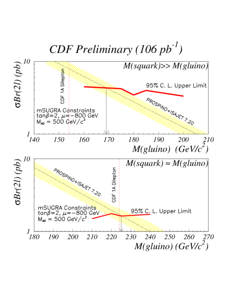
Figure 26: CDF 95% C.L. upper limits cdf1_2ljmet on $\sigma\cdot Br$ as a function of $M(\mbox{$\tilde{g}$})$, compared to NLO predictions prospino-k in the MSSM framework at $\tan\beta$ = 2 and $\mu=-800$ $\;{\rm GeV}/c^{2}$ for two cases: (i) $M(\mbox{$\tilde{q}$})\gg M(\mbox{$\tilde{g}$})$ and (ii) $M(\mbox{$\tilde{q}$})\simeq M(\mbox{$\tilde{g}$})$. The nominal value of the cross section for $\tilde{g}$$\tilde{g}$, $\tilde{g}$$\tilde{q}$, $\tilde{q}$$\bar{\tilde{q}}$, and $\tilde{q}$$\tilde{q}$ production is calculated with CTEQ3M parton distribution function at $Q^{2}$ = $M^{2}$. The band shows the theoretical uncertainty in the calculation varying $Q^{2}$ between $(2M)^{2}$ and $(0.5M)^{2}$.

Table 8: Approximate estimate ofmSUGRA (isajet version 7.20) points corresponding to results of the CDF LS dilepton analysis for (i) $M(\mbox{$\tilde{q}$})\gg M(\mbox{$\tilde{g}$})$ and (ii) $M(\mbox{$\tilde{q}$})\simeq M(\mbox{$\tilde{g}$})$. Other mSUGRA parameters are fixed as $\tan\beta=2$, $\mu<0$ and $A_{0}=0$. SUSY masses and SUGRA parameters are given in $\;{\rm GeV}/c^{2}$.

Mass	(i)	(ii)
$\tilde{q}$	502	223
$\tilde{g}$	169	225
$\tilde{\chi}_{1}^{\pm}$	50	78
mSUGRA
$m_{0}$	490	120
$m_{1/2}$	47	73
$\mu$	$-437$	$-169$

XII.4.2 DØ Searches

Jets and Missing Transverse Energy

The DØ search for $\tilde{g}$$\tilde{g}$, $\mbox{$\tilde{q}$}\bar{\mbox{$\tilde{q}$}}$, and $\tilde{g}$$\tilde{q}$ production in the jets + ${E\!\!\!\!/_{T}}$ channel is based on 72 ${\rm pb}^{-1}$ of data d0jmet1b ; d0jmet1a taken during the 1994-95 run. The cross section values are determined using the NLO calculation in Ref. prospino-k by assuming degeneracy of five of the squarks; top squarks are excluded in this analysis.

The analysis requires three jets with $E_{T}$$>$ 25 GeV, where the leading jet has $E_{T}$$>$ 115 GeV and $|\eta|$$<$1.1. The jet angle, with respect to the hard scattering vertex, is confirmed using the tracks associated with the leading jet; this is because an average event is likely to have more than one interaction and choosing the incorrect vertex will lead to significant spurious ${E\!\!\!\!/_{T}}$. The ${E\!\!\!\!/_{T}}$ is required to be greater than 75 GeV to stay above the trigger threshold. The jet energy has a large resolution ($\sigma=0.8\sqrt{\mbox{$p_{T}$}}$) thus events where the ${E\!\!\!\!/_{T}}$ is correlated with the jets in azimuth are removed. To remove events that are likely background, any candidates with isolated electrons or muons are removed from the sample. This cut reduces backgrounds due to vector boson production in association with jets and $t\overline{t}$ production. The vector boson backgrounds are simulated with vecbos vecbos and the $t\overline{t}$ background with herwig herwig . The multijet background is determined from a data set taken without a ${E\!\!\!\!/_{T}}$ term in the trigger. The ${E\!\!\!\!/_{T}}$ distribution is fit and extrapolated into the region of interest for this analysis, i.e. greater than 75 GeV. The cuts on ${E\!\!\!\!/_{T}}$ and $H_{T}$, where $H_{T}$ is the scalar sum of the non-leading jets, are optimized for significance at each point in parameter space. At the lowest ${E\!\!\!\!/_{T}}$ and $H_{T}$ point, ${E\!\!\!\!/_{T}}$$>$ 75 GeV and $H_{T}$$>$ 100 GeV, the number of events observed is 15 with an expected background of $8.3\pm 3.4$. The probability to observe more than 15 events, given this background estimation, is 9.2%. We interpret this result as an exclusion contour in the $m_{0}$ and $m_{1/2}$ plane for $\tan\beta=2$, $A_{0}=0$, and $\mu<0$ (see Fig. 27). At low $m_{0}$, gluinos with masses less than 300 $\;{\rm GeV}/c^{2}$ are excluded. At the $m_{0}$ and $m_{1/2}$ point where the squark and gluino masses are equal this analysis excludes masses less than 260 $\;{\rm GeV}/c^{2}$.

Figure 27: DØ 95% C.L. exclusion contour (heavy line) in the $m_{1/2}$-$m_{0}$ plane ($\tan\beta=2$, $A_{0}=0$, and $\mu<0$) for the jets + ${E\!\!\!\!/_{T}}$ search. The thin lines are contours of constant gluino or squark mass. The dark shaded area is where mSUGRA does not predict electroweak symmetry breaking or the sneutrino is the LSP.

Dileptons, Jets, and Missing Transverse Energy

The DØ search for $\tilde{g}$$\tilde{g}$, $\mbox{$\tilde{q}$}\bar{\mbox{$\tilde{q}$}}$, and $\tilde{g}$$\tilde{q}$ production in the dielectron + jets + ${E\!\!\!\!/_{T}}$ channel is based on 108 ${\rm pb}^{-1}$ d0dilep taken during the 1992-95 run. Top squarks are excluded in this analysis. The cross section values are determined using the LO calculation from Ref. spythia-k .

The dilepton modes used are electron-electron ($ee$), electron-muon ($e\mu$), and muon-muon ($\mu\mu$). In order to optimize the ratio of signal to background several kinematic thresholds for the leptons, jets, and ${E\!\!\!\!/_{T}}$ are employed. The $ee$ channel requires two electrons with $\mbox{$E_{T}$}>17$ and 15 GeV. The $e\mu$ requires an electron with $\mbox{$E_{T}$}>17$ GeV and a muon with $\mbox{$p_{T}$}>$ 4, 7, or 10 $\;{\rm GeV}/c$. The $\mu\mu$ channel requires two muons with $\mbox{$p_{T}$}>20$ and 10 $\;{\rm GeV}/c$. Each dilepton channel also requires two jets and ${E\!\!\!\!/_{T}}$. The jet cuts are also variable with $\mbox{$E_{T}$}>20$ or 45 GeV. The ${E\!\!\!\!/_{T}}$ is required to be greater than 20, 30, or 40 GeV. In addition, events with a dilepton invariant mass near the $Z$ mass are sometimes rejected. At different points in $m_{0}$-$m_{1/2}$ space a fast Monte Carlo, interfaced with spythia spythia-k , is used to predict which set of thresholds on the $ee,e\mu$, and $\mu\mu$ channels give the greatest significance. The set of cuts at each point are then applied to the data and compared to the expected background. The maximum significance is taken from $ee$, $e\mu$, and $\mu\mu$ channels separately, from the combination of any two-channels, or three-channels. The backgrounds are due to $W$ boson, $Z$ boson, $t\overline{t}$, and QCD. The $W$ boson, $Z$ boson, and $t\overline{t}$ backgrounds are included in the fast Monte Carlo with the cross sections normalized to the DØ measured values. The QCD and vector boson background is taken from data. No excess of events over background is observed and the result is presented as a limit in the $m_{1/2}$-$m_{0}$ plane for $A_{0}=0$, $\mu<0$, and at $\tan\beta=2,3,4,5$, and 6. (see Fig. 28). For equal $\tilde{q}$ and $\tilde{g}$ masses a limit of 270 GeV is obtained. In Fig. 28 the mass limits are reduced because as $\tan\beta$ increases the branching ratio into first and second generation leptons decreases.

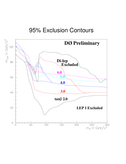
Figure 28: DØ 95% C.L. exclusion contour in the $m_{1/2}$-$m_{0}$ plane ($A_{0}=0$ and $\mu<0$) for the dielectron + jets + ${E\!\!\!\!/_{T}}$ search. The values of $\tan\beta$ vary from 2 to 6, where the strictest limits come from $\tan\beta=2$ and decrease as $\tan\beta$ increases. Also shown are the limits from LEP I for the same $\tan\beta$ values.

XII.5 Search for Sbottom and Stop Quarks

At the Tevatron, the third generation scalar quarks are produced in pairs via $gg$ and $q\overline{q}$ fusion. The leading order terms in the production cross sections depend only on the scalar quark masses. In the NLO terms, the largest theoretical uncertainty is due to the QCD $\mu$ scale. The dominant SUSY corrections depend on other scalar quark masses and are small ($\sim 1\%$). For example, a third generation scalar quark ($\tilde{Q}_{1}$ = $\tilde{b}_{1}$ or $\tilde{t}_{1}$) with a mass of 110 $\;{\rm GeV}/c^{2}$ would have a production cross section of 7.4$\pm$1.1 pb, using the mass scale $\mu=M(\tilde{Q}_{1})$ for the central value and $\mu=M(\tilde{Q}_{1})/2$ and $\mu=2M(\tilde{Q}_{1})$ for the uncertainties susy_nlo_xsec2 .

XII.5.1 Search for Sbottom and Stop Quarks in ${E\!\!\!\!/_{T}}$+ Jets Channel

DØ and CDF search for direct production of $\tilde{b}_{1}$$\bar{\tilde{b}}_{1}$ and $\tilde{t}_{1}$$\bar{\tilde{t}}_{1}$ in the ${E\!\!\!\!/_{T}}$ + jets channel:

• For the sbottom search we consider the $\tilde{b}_{1}\rightarrow b\tilde{\chi}_{1}^{0}$ decay mode. Since this is a tree-level decay it dominates over most of the parameter space if $\tilde{\chi}_{2}^{0}$ is heavier than $\tilde{b}_{1}$.

• In the absence of flavor changing neutral currents the $\mbox{$\tilde{t}_{1}$}\rightarrow c\mbox{$\tilde{\chi}_{1}^{+}$}$ decay proceeds via a one-loop diagram and will become dominant when the tree-level decay $\tilde{t}_{1}\rightarrow b\tilde{\chi}_{1}^{+}$ is kinematically forbidden.

Thus, $Br(\mbox{$\tilde{b}_{1}$}\rightarrow b\mbox{$\tilde{\chi}_{1}^{0}$})=100\%$ and $Br(\mbox{$\tilde{t}_{1}$}\rightarrow c\mbox{$\tilde{\chi}_{1}^{0}$})=100\%$ are assumed. Both analyses use the cross sections for $\tilde{b}_{1}$$\tilde{b}_{1}$ and $\tilde{t}_{1}$$\tilde{t}_{1}$ production calculated at NLO susy_nlo_xsec2 in setting the lower limits on the sbottom and stop masses.

DØ Search for Sbottom Quark

DØ has searched for sbottom quarks in four channels sbottom_d0 , which are combined to set limits on the production of sbottom quarks. The first required a ${E\!\!\!\!/_{T}}$+jets topology, while the other three channels impose the additional requirement that at least one jet have an associated muon, which was used to tag $b$ quark decay. For all channels, the presence of significant ${E\!\!\!\!/_{T}}$ was used to identify the non-interacting LSPs. Backgrounds arose from events where neutrinos produced significant ${E\!\!\!\!/_{T}}$; for example, in $W$ plus multijet events where $W\rightarrow\ell\nu$.

Events for the ${E\!\!\!\!/_{T}}$+jets channel were collected using a trigger which required ${E\!\!\!\!/_{T}}$$>35$ GeV. During offline analysis, events with two jets ($E_{T}^{\rm jet}>30$ GeV), ${E\!\!\!\!/_{T}}$$>40$ GeV, and no isolated electrons or muons were selected. To eliminate QCD backgrounds, additional cuts were made on the angles between the two jets, and between jets and the ${E\!\!\!\!/_{T}}$ direction. Data with an integrated luminosity of 7.4 pb^-1 yielded three events satisfying the selection criteria with and expected background of $3.5\pm 1.2$ stop_d0 .

The muon channel used a combination of three triggers. The triggers had the following requirements: a trigger with two low-$p_{T}$ muons ($p_{T}^{\mu}>3.0$ GeV/c), a trigger with a single low-$p_{T}$ muon plus a jet with $E_{T}>10$ GeV, or a trigger which required a high-$p_{T}$ muon ($p_{T}^{\mu}>15$ GeV/c) plus a jet with $E_{T}>15$ GeV. Integrated luminosities of 60.1 $\;{\rm pb}^{-1}$, 19.5 $\;{\rm pb}^{-1}$, and 92.4 $\;{\rm pb}^{-1}$, respectively were collected using the three muon triggers. Either two muons, each associated with its own jet, or a single jet-associated muon was required. If the event had only one muon-jet combination, an additional jet with $E_{T}>25$ GeV was required. To remove QCD backgrounds, events were selected with ${E\!\!\!\!/_{T}}$ $>35$ GeV and an azimuthal angular separation between the ${E\!\!\!\!/_{T}}$ direction and the nearest jet greater than 0.7 radians. For the single muon channels, backgrounds from $W$ boson decays were removed by cuts on the muon-jet correlation; and top backgrounds were minimized by cuts on the scalar sum of jet $E_{T}$. Following all selection criteria, two events remained in the data.

Combining the four channels gave five events observed in the data with a total background estimated to be $6.0\pm 1.3$ events (1.4 $t\bar{t}$, 4.0 $W$ boson, and 0.6 $Z$ boson).

We set limits on the cross section by combining the acceptances and integrated luminositiees for the different channels. For any given $M(\mbox{$\tilde{b}_{1}$})$, we determined the value of $M(\mbox{$\tilde{\chi}_{1}^{0}$})$ where our 95% C.L. limit intersected the theoretical cross section, and excluded the region where the cross section was greater than our limit. We used the program prospino prospino-k to calculate the theoretical sbottom pair production cross section as a function of $M(\mbox{$\tilde{b}_{1}$})$.

CDF Searches for Stop and Sbottom Quarks

The CDF analysis begins with a sample of events collected using a trigger which required uncorrected missing transverse energy ${E\!\!\!\!/_{T}}$ $>$ 35 GeV, corresponding to 88.0 $\pm$ 3.6 $\;{\rm pb}^{-1}$ cdf1_stopsbot .

We select events with 2 or 3 jets which have uncorrected transverse energy $E_{T}$ $>$ 15 GeV and $|\eta|<2$, requiring that there are no other jets in the events with $E_{T}$ $>$ 7 GeV and $|\eta|<3.6$. Jets are found from calorimeter information using a fixed cone algorithm with a cone radius of 0.4 in $\eta$-$\phi$ space. The ${E\!\!\!\!/_{T}}$ cut is increased beyond the trigger threshold to 40 GeV. To reduce the contribution from processes where missing energy comes from jet energy mismeasurement we require that the ${E\!\!\!\!/_{T}}$ direction is neither parallel to any jet ($j$) nor anti-parallel to the leading $E_{T}$ jet: $min\Delta\phi(\mbox{${E\!\!\!\!/_{T}}$},j)>45\mbox{${}^{\circ}$}$, $\Delta\phi(\mbox{${E\!\!\!\!/_{T}}$},j_{1})<165\mbox{${}^{\circ}$}$, where the jet indices are ordered by decreasing $E_{T}$. A further reduction in the QCD multijet background is made by requiring that $45\mbox{${}^{\circ}$}<\Delta\phi(j_{1},j_{2})<165\mbox{${}^{\circ}$}$. We reject events with one or more identified electrons (muons) with $E_{T}$ ($p_{T}$) $>$ 10 GeV ($\;{\rm GeV}/c$).

After applying all these requirements, the data sample (called the pretagged sample) contains 396 events. The largest source of background in the sample is the production of $W$+jets, where the $W$ boson decays to a neutrino and an electron or muon that is not identified, or a tau which decays hadronically. The sample also contains QCD multijet events where the large ${E\!\!\!\!/_{T}}$ is due to jet energy mismeasurement.

The SVX^′ information is used to tag heavy flavor jets. We associate tracks to a jet by requiring that the track is within a cone of 0.4 in $\eta$-$\phi$ space around the jet axis. We require tracks to have $p_{T}$ $>$1.0 $\;{\rm GeV}/c$, positive impact parameter, and a good SVX^′ hit pattern. A good SVX^′ hit pattern consists of 3 or 4 hits in the SVX^′ detector with no hits shared by other tracks. The impact parameter of a track is positive if its projection on the jet axis is positive, and negative otherwise.

For each track the probability that the track comes from the primary vertex is determined taking into account the impact parameter resolution function. The resolution function is measured from the negative impact parameter signature distribution in the data, which does not carry lifetime information. We call this probability the track probability. By construction, the distribution is flat for tracks originating from the primary vertex. For tracks from a secondary vertex, the distribution peaks near zero. The joint probability for tracks associated to a jet is called the jet probability (${\cal P}_{jet}$) cdf_mu_bjet . The jet probability is flat for a primary jet data sample by construction. For bottom and charm jets, the jet probability peaks near zero.

We select events for the stop search analysis by requiring that the event have at least one jet with ${\cal P}_{jet}$ $<$ 0.05. This rejects 97% of the background while its efficiency for signal events is 25% . For the sbottom search analysis, we require the event to have at least one jet with ${\cal P}_{jet}$ $<$ 0.01. This rejects 99% of the background while retaining 45% of the sbottom events.

In the sbottom (stop) analysis, we observe 5 (11) events in data, which is consistent with $5.8\pm 1.8$ ($14.5\pm 4.2$) events expected from the Standard Model processes such as $W$ and $Z$ production, $t\overline{t}$ production, diboson production, and QCD events.

The sources of systematic uncertainty on the expected signal, which are common to both sbottom and stop analyses, are (i) theoretical uncertainty on the NLO cross section for squark production, (ii) initial and final state gluon radiation, (iii) uncertainty on the efficiency for the heavy flavor tagging, (iv) jet energy scale, (v) uncertainty on the trigger efficiency, (vi) uncertainty on the degradation of the signal efficiency for events with multiple primary vertices, (vii) uncertainty on the integrated luminosity and (viii) MC statistics. The total systematic uncertainty ranges from 31% to 36% for the mass range 30 $\;{\rm GeV}/c^{2}$ to 150 $\;{\rm GeV}/c^{2}$. Using a background-subtracted method bs_method , we find an exclusion region in the $M(\mbox{$\tilde{\chi}_{1}^{0}$})$-$M(\tilde{Q}_{1})$ plane at 95% C.L. limit.

CDF and DØ Exclusion Regions

The excluded regions from CDF and DØ in the $M(\mbox{$\tilde{\chi}_{1}^{0}$})$-$M(\mbox{$\tilde{b}_{1}$})$ plane are shown in Fig. 29. Also plotted are the latest results from ALEPH stopsbot_lep189 . The maximum $M(\mbox{$\tilde{b}_{1}$})$ excluded is 148 $\;{\rm GeV}/c^{2}$ for $M(\mbox{$\tilde{\chi}_{1}^{0}$})=0\ \mbox{$\;{\rm GeV}/c^{2}$}$ by CDF and 115 $\;{\rm GeV}/c^{2}$ for $M(\mbox{$\tilde{\chi}_{1}^{0}$})<20\ \mbox{$\;{\rm GeV}/c^{2}$}$ by DØ.

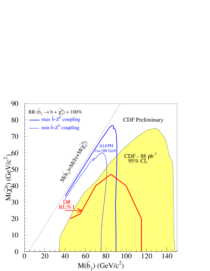
Figure 29: CDF and DØ 95% C.L. exclusion contours in the $M(\mbox{$\tilde{\chi}_{1}^{0}$})$-$M(\tilde{b}_{1})$ plane for $\mbox{$\tilde{b}_{1}$}\rightarrow b\mbox{$\tilde{\chi}_{1}^{0}$}$. Also shown are the exclusion contours from the ALEPH experiment at LEP for minimal and maximal couplings stopsbot_lep189 .

Figure 30 shows the exclusion region for the stop analyses from CDF and DØ, compared to the ALEPH result stopsbot_lep189 . The DØ results are based on 7.4 $\;{\rm pb}^{-1}$ stop_d0 . The maximum $M(\mbox{$\tilde{t}_{1}$})$ excluded is 119 $\;{\rm GeV}/c^{2}$ for $M(\mbox{$\tilde{\chi}_{1}^{0}$})=40\ \mbox{$\;{\rm GeV}/c^{2}$}$ by CDF. The maximum value of the neutralino mass is 51 $\;{\rm GeV}/c^{2}$ which corresponds to the stop mass of 102 $\;{\rm GeV}/c^{2}$.

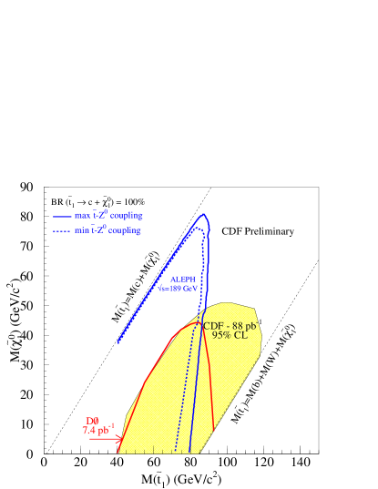
Figure 30: CDF and DØ 95% C.L. exclusion contours in the $M(\mbox{$\tilde{\chi}_{1}^{0}$})$-$M(\tilde{t})$ plane for $\mbox{$\tilde{t}_{1}$}\rightarrow c\mbox{$\tilde{\chi}_{1}^{0}$}$. Also shown are the exclusion contours from the ALEPH experiment at LEP for minimal and maximal couplings stopsbot_lep189 .

One can investigate the results within mSUGRA framework b-dutta . For the sbottom case, the $\tan\beta$ value has to be larger to generate light sbottom mass. There is little mSUGRA parameter space to satisfy $M(\mbox{$\tilde{\chi}_{2}^{0}$})\approx M(\mbox{$\tilde{\chi}_{1}^{\pm}$})>M(\mbox{$\tilde{b}_{1}$})$. For example, an MSSM point of $M(\mbox{$\tilde{b}_{1}$})\approx 100\ \mbox{$\;{\rm GeV}/c^{2}$}$ and $M(\mbox{$\tilde{\chi}_{1}^{0}$})\approx 50\ \mbox{$\;{\rm GeV}/c^{2}$}$ is excluded in the CDF analysis. The corresponding mSUGRA point is $m_{0}=134\ \mbox{$\;{\rm GeV}/c^{2}$},m_{1/2}=130\ \mbox{$\;{\rm GeV}/c^{2}$},\tan\beta=45,\mu>0,A_{0}=-655\ \mbox{$\;{\rm GeV}/c^{2}$}$, which generates $M(\mbox{$\tilde{b}_{1}$})=98\ \mbox{$\;{\rm GeV}/c^{2}$}$, $M(\mbox{$\tilde{\chi}_{1}^{0}$})=53\ \mbox{$\;{\rm GeV}/c^{2}$}$, and $M(\mbox{$\tilde{\chi}_{1}^{\pm}$})=98\ \mbox{$\;{\rm GeV}/c^{2}$}$. However, the problem is that the electroweak symmetry does not break radiatively. In contrast with the sbottom case, the light stop mass can be generated in lower $\tan\beta$ values. One of such mSUGRA points is $m_{0}=130\ \mbox{$\;{\rm GeV}/c^{2}$},m_{1/2}=125\ \mbox{$\;{\rm GeV}/c^{2}$},\tan\beta=7,\mu>0,A_{0}=-535\ \mbox{$\;{\rm GeV}/c^{2}$}$, which generates $M(\mbox{$\tilde{t}_{1}$})=88\ \mbox{$\;{\rm GeV}/c^{2}$}$, $M(\mbox{$\tilde{\chi}_{1}^{0}$})=49\ \mbox{$\;{\rm GeV}/c^{2}$}$, and $M(\mbox{$\tilde{\chi}_{1}^{\pm}$})=89\ \mbox{$\;{\rm GeV}/c^{2}$}$.

XII.5.2 Search for Stop Quark in Lepton+${E\!\!\!\!/_{T}}$+jets Channel

The CDF search for evidence of direct production of $\tilde{t}_{1}$$\bar{\tilde{t}}_{1}$ in the lepton+${E\!\!\!\!/_{T}}$+jets channel is based on 88 $\;{\rm pb}^{-1}$of inclusive lepton ($e$ and $\mu$) data cdf1_stop_ljmet ; cdf1_stop_ljmet2 . Two separate $\tilde{t}_{1}$ decay channels were investigated. In the first channel, we look for $\tilde{t}_{1}\rightarrow b\tilde{\chi}_{1}^{+}$ (with a branching ratio of 100%). We then require one of the charginos, which decay via a virtual $W^{\pm}$, to decay as $\tilde{\chi}_{1}^{+}\rightarrow e^{+}\nu~{}\tilde{\chi}_{1}^{0}$ or $\mu^{+}\nu~{}\tilde{\chi}_{1}^{0}$ with an assumed branching ratio of 11% for each lepton type. For models where $\tilde{t}_{1}\rightarrow b\tilde{\chi}_{1}^{+}$ is not kinematically allowed, we considered a second decay scenario in which $\mbox{$\tilde{t}_{1}$}~{}\rightarrow bl^{+}\tilde{\nu}$, where $\tilde{\nu}$ is a scalar neutrino and each $l=e,~{}\mu,~{}\tau$ has a branching ratio of 33.3%. In our two scenarios, either the $\tilde{\chi}_{1}^{0}$ or the $\tilde{\nu}$ is the LSP. For either process the signature is an isolated lepton, missing transverse energy, ${E\!\!\!\!/_{T}}$ from the LSP’s, and two jets from the $b$ quarks.

The data for this analysis was obtained by requiring (i) an electron with $E_{T}\geq$ 10 $\;{\rm GeV}/c$ or muon with $p_{T}\geq$ 10 $\;{\rm GeV}/c$ originating from the primary vertex and passing lepton identification cuts, (ii) $\mbox{${E\!\!\!\!/_{T}}$}\geq$ 25 GeV, and (iii) at least two jets, one with $E_{T}\geq$ 12 GeV and the second with $E_{T}\geq$ 8 GeV. The lepton identification cuts were identical to those used in previous CDF analyses cdftop94 . We also required the leptons to pass an isolation cut in which the calorimeter $E_{T}$ in a cone of $\Delta R=0.4$ around the lepton was less than 2 GeV (excluding the lepton $E_{T}$).

We used the SVX^′ to identify secondary vertices from $b$ quark decays and selected events with at least one secondary vertex. The tagging algorithm is described in Ref. cdftop94 with improvements given in Ref. cdftop95 . We reduced the $Z/\gamma\rightarrow l^{+}l^{-}$ background in our sample by removing events with either two isolated, opposite-sign leptons or an isolated lepton that reconstructs an invariant mass $\geq$ 50 $\;{\rm GeV}/c^{2}$ with a second CTC track with no lepton identification requirements. Finally, we reduced the background from $b\overline{b}$ events and events with hadrons misidentified as leptons (fake leptons) by requiring that the $\Delta\phi$ between the ${E\!\!\!\!/_{T}}$ and the nearer of the two highest-$E_{T}$ jets be $\geq$ 0.5 rad. This reduces fake ${E\!\!\!\!/_{T}}$ which is the result of jet energy mismeasurement. The number of events remaining in our sample after all cuts is 81.

Signal event samples were created using isajet version 7.20 tk-isajet . The supersymmetric particle masses used in signal simulation were: $M(\tilde{\chi}_{1}^{\pm})=$ 90 $\;{\rm GeV}/c^{2}$, $M(\tilde{\chi}_{1}^{0})=$ 40 $\;{\rm GeV}/c^{2}$, and $M(\tilde{\nu})\geq$ 40 $\;{\rm GeV}/c^{2}$. The sources of uncertainty for signal selection efficiency are (i) the $b$-jet tagging efficiency, (ii) the trigger efficiencies, (iii) the integrated luminosity, (iv) initial- and final-state radiation, (v) Monte Carlo statistics, (vi) the parton distribution function, (vii) the corrections to jet energies from the underlying event, (viii) the jet energy scale, and (ix) the lepton identification and isolation efficiencies. The effects of some of these sources vary with $M(\mbox{$\tilde{t}_{1}$})$, but none contribute more than 10% to the overall uncertainty, which is less than 16% for all $M(\mbox{$\tilde{t}_{1}$})$ considered.

The number of background events from heavy flavor quark production were predicted using measured or calculated cross sections and selection efficiencies determined from Monte Carlo. Top-pair and single-top production were simulated using herwig version 5.6 herwig with $\sigma_{t\bar{t}}$ = 5.1 $\pm$ 1.6  pb top_prod for $M(t)$ = 175 $\;{\rm GeV}/c^{2}$. The value of $\sigma_{t\bar{b}}$ from $W$-gluon fusion for $M(t)$ = 175 $\;{\rm GeV}/c^{2}$ from a NLO calculation is 1.70 $\pm$ 0.15  pb stelzer . Vector boson samples were generated using vecbos version 3.03 vecbos . Drell-Yan, $b\bar{b}$, and $c\bar{c}$ samples were generated with isajet version 7.06 and normalized to independent CDF data samples.

To determine the number of events with fake leptons in our sample, we used a data sample passing all our selection cuts with the exceptions of a non-overlapping ${E\!\!\!\!/_{T}}$ requirement ($15\leq\mbox{${E\!\!\!\!/_{T}}$}\leq 20$ GeV) and no requirement on $\Delta\phi$(${E\!\!\!\!/_{T}}$, nearer jet). The number of fake lepton events was normalized to this data sample, which contained negligible signal, after other backgrounds were subtracted. The number of fake lepton events was then extrapolated to the signal region using cut efficiencies determined from an independent fake-lepton event sample.

The significant backgrounds are $t\overline{t}$, $b\overline{b}$, $W^{\pm}\rightarrow l^{+}\nu~{}+\geq$2 jets, and fake lepton events. The number of data events agrees well with the expected background.

To determine the number of potential signal events in this final data sample, we performed extended, unbinned likelihood fits for each $\tilde{t}_{1}$ mass considered for both decay scenarios. The likelihood fits compared the shapes of distributions of the signal and background and included Gaussian terms tying the fit background levels to their predicted levels. The fit parameters were the number of signal events, the number of $t\overline{t}$ events, the number of $b\overline{b}$ plus fake lepton events, and the number of vector boson events (represented in the fit by the $W^{\pm}\rightarrow l^{+}\nu~{}+\geq$2 jets distributions).

For the $\tilde{t}_{1}\rightarrow b\tilde{\chi}_{1}^{+}$ decay, sensitivity to signal was greatest for a two-dimensional fit to the combined probability distributions for $H_{T}$ and $\Delta\phi(j_{1},j_{2})$. Fit results at all masses were consistent with zero signal events. The 95% C.L. limits on $\sigma_{\mbox{$\tilde{t}_{1}$}\mbox{$\bar{\tilde{t}}_{1}$}}$ for this decay are shown in Fig. 31 as a function of $M(\mbox{$\tilde{t}_{1}$})$. The NLO theoretical prediction for $\sigma_{\mbox{$\tilde{t}_{1}$}\mbox{$\bar{\tilde{t}}_{1}$}}$ using the renormalization scale $\mu=M(\mbox{$\tilde{t}_{1}$})$ and parton distribution function CTEQ3M is shown in Fig. 31 for comparison susy_nlo_xsec2 .

For the $\mbox{$\tilde{t}_{1}$}~{}\rightarrow bl^{+}\tilde{\nu}$ decay scenario, sensitivity to signal was greatest for a fit to the $H_{T}$ distribution. Again, all fit results were consistent with zero signal events. The 95% C.L. limits on $\sigma_{\mbox{$\tilde{t}_{1}$}\mbox{$\bar{\tilde{t}}_{1}$}}$ for the $\mbox{$\tilde{t}_{1}$}~{}\rightarrow bl^{+}\tilde{\nu}$ decay were generated for $M(\tilde{\nu})$ between 40 and 50 $\;{\rm GeV}/c^{2}$, and the resulting region in the $M(\tilde{\nu})$-$M(\mbox{$\tilde{t}_{1}$})$ plane for which the limit on $\sigma_{\mbox{$\tilde{t}_{1}$}\mbox{$\bar{\tilde{t}}_{1}$}}$ is less than the NLO prediction ($\mu=M(\mbox{$\tilde{t}_{1}$})$) is shown in Fig. 32.

Figure 31: The points represent the CDF 95% C.L. cross section limit as a function of $\tilde{t}_{1}$ mass in the model where the decay $\tilde{t}_{1}\rightarrow b\tilde{\chi}_{1}^{\pm}$ has a branching ratio of 100% cdf1_stop_ljmet . The masses in the model were $M(\tilde{\chi}_{1}^{\pm})=$ 90 $\;{\rm GeV}/c^{2}$ and $M(\tilde{\chi}_{1}^{0})=$ 40 $\;{\rm GeV}/c^{2}$. The line without markers represents the NLO theoretical prediction for $\sigma_{\mbox{$\tilde{t}_{1}$}\mbox{$\bar{\tilde{t}}_{1}$}}$ using the renormalization scale $\mu=M(\mbox{$\tilde{t}_{1}$})$ and parton distribution function CTEQ3M. The dashed lines represent the NLO cross section for $\mu=M(\mbox{$\tilde{t}_{1}$})/2$ and $\mu=2M(\mbox{$\tilde{t}_{1}$})$.

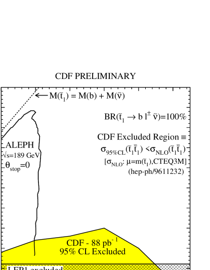
Figure 32: CDF 95% C.L. excluded region in the $M(\tilde{\nu})$-$M(\mbox{$\tilde{t}_{1}$})$ plane when the $\mbox{$\tilde{t}_{1}$}~{}\rightarrow be^{+}\tilde{\nu}$, $\mbox{$\tilde{t}_{1}$}~{}\rightarrow b\mu^{+}\tilde{\nu}$, and $\mbox{$\tilde{t}_{1}$}~{}\rightarrow b\tau^{+}\tilde{\nu}$ branching ratios are assumed to be 33.3% cdf1_stop_ljmet2 . We define the exclusion region as that region of supersymmetric parameter space for which the 95% C.L. limit on $\sigma_{\mbox{$\tilde{t}_{1}$}\mbox{$\bar{\tilde{t}}_{1}$}}$ is less than the NLO theoretical prediction ($\mu=M(\mbox{$\tilde{t}_{1}$})$). The LEP1 limit on $M(\tilde{\nu})$ and ALEPH excluded region in the $M(\tilde{\nu})$-$M(\mbox{$\tilde{t}_{1}$})$ plane are also shown aleph . The ALEPH excluded region corresponds to the case in which the $\tilde{t}_{1}$ decouples from the $Z^{0}$ ($\theta_{\mbox{$\tilde{t}_{1}$}}=$ 0.98 rad).

XII.6 Summary

The CDF and DØ collaborations have actively carried out analyses of various SUSY signatures in the MSSM or mSUGRA framework. We describe the most up-to-date analyses. A summary of the SUSY mass limits is given in Table 9. There are several analyses which are in progress and are not included in this paper. The status of the SUSY analyses using the Run Ia+Ib data is summarized in Table 10.

Table 9: Summary of 95% C.L. lower mass limits on SUSY particles in mSUGRA or MSSM framework. The strongest limits from CDF and DØ are listed.

Decay	Mass Limit ($\;{\rm GeV}/c^{2}$)			$m_{1/2}$	$m_{0}$	$\tan\beta$	$sgn(\mu)$	$A_{0}$
mSUGRA
$\mbox{$\tilde{\chi}_{1}^{\pm}$}\mbox{$\tilde{\chi}_{2}^{0}$}\rightarrow 3\ell+X$	$\tilde{\chi}_{1}^{+}$	62	(106 $\;{\rm pb}^{-1}$)	50	160	2	$-1$	0
$\mbox{$\tilde{g}$}\mbox{$\tilde{g}$},\mbox{$\tilde{g}$}\mbox{$\tilde{q}$},\mbox{$\tilde{q}$}\mbox{$\bar{\tilde{q}}$}\rightarrow jets+\mbox{${E\!\!\!\!/_{T}}$}$	$\tilde{g}$	300	( 72 $\;{\rm pb}^{-1}$)	105	0	2	$-1$	0
$\mbox{$\tilde{g}$}\mbox{$\tilde{g}$},\mbox{$\tilde{g}$}\mbox{$\tilde{q}$},\mbox{$\tilde{q}$}\mbox{$\bar{\tilde{q}}$}\rightarrow 2\ell+jets+\mbox{${E\!\!\!\!/_{T}}$}$	$\tilde{g}$	270	(108 $\;{\rm pb}^{-1}$)	89	150	2	$-1$	0
$\mbox{$\tilde{g}$}\mbox{$\tilde{g}$},\mbox{$\tilde{g}$}\mbox{$\tilde{q}$},\mbox{$\tilde{q}$}\mbox{$\bar{\tilde{q}}$}\rightarrow 2\ell+jets+\mbox{${E\!\!\!\!/_{T}}$}$	$\tilde{g}$ (heavy $\tilde{q}$)	169	(106 $\;{\rm pb}^{-1}$)	50	500	2	$-1$	0
$\mbox{$\tilde{b}_{1}$}\rightarrow b+\mbox{$\tilde{\chi}_{1}^{0}$}$	$\tilde{b}_{1}$	—	( 88 $\;{\rm pb}^{-1}$)	not available in mSUGRA
$\mbox{$\tilde{t}_{1}$}\rightarrow c+\mbox{$\tilde{\chi}_{1}^{0}$}$	$\tilde{t}_{1}$	90	( 88 $\;{\rm pb}^{-1}$)	125	130	7	+1	$-535$
MSSM
$\mbox{$\tilde{b}_{1}$}\rightarrow b+\mbox{$\tilde{\chi}_{1}^{0}$}(40\ \mbox{$\;{\rm GeV}/c^{2}$})$	$\tilde{b}_{1}$	140	( 88 $\;{\rm pb}^{-1}$)
$\mbox{$\tilde{t}_{1}$}\rightarrow c+\mbox{$\tilde{\chi}_{1}^{0}$}(40\ \mbox{$\;{\rm GeV}/c^{2}$})$	$\tilde{t}_{1}$	119	( 88 $\;{\rm pb}^{-1}$)
$\mbox{$\tilde{t}_{1}$}\rightarrow b+l+\mbox{$\tilde{\chi}_{1}^{0}$}(40\ \mbox{$\;{\rm GeV}/c^{2}$})$	$\tilde{t}_{1}$	125	( 88 $\;{\rm pb}^{-1}$)

Table 10: Status (as of June 1999) of SUSY analyses in MSSM or SUGRA framework at CDF and DØ using the Run Ib (or Run Ia+Ib) data.

Prod.	SUGRA Signature	CDF	DØ
	$(\ell^{\pm}\nu\;\mbox{$\tilde{\chi}_{1}^{0}$})\;(\ell^{+}\ell^{-}\;\mbox{$\tilde{\chi}_{1}^{0}$})$	cdf_tril	d0_tril
$\tilde{\chi}_{1}^{\pm}$$\tilde{\chi}_{2}^{0}$	$(\ell^{\pm}\nu\;\mbox{$\tilde{\chi}_{1}^{0}$})\;(\tau^{+}\tau^{-}\;\mbox{$\tilde{\chi}_{1}^{0}$})$	Progress
	$(\tau^{\pm}\nu\;\mbox{$\tilde{\chi}_{1}^{0}$})\;(\ell^{+}\ell^{-}\;\mbox{$\tilde{\chi}_{1}^{0}$})$	Progress
$\mbox{$\tilde{g}$}\mbox{$\tilde{g}$},\mbox{$\tilde{q}$}\mbox{$\tilde{g}$},\mbox{$\tilde{q}$}\bar{\mbox{$\tilde{q}$}}$	${E\!\!\!\!/_{T}}$$+\geq$3,4 jets	Progress	d0jmet1b
$\tilde{g}$$\tilde{g}$	$(q\bar{q}^{\prime}\mbox{$\tilde{\chi}_{1}^{\pm}$})\;(q\bar{q}^{\prime}\mbox{$\tilde{\chi}_{1}^{\pm}$})\rightarrow\ell^{\pm}\ell^{\pm}$ + jets + ${E\!\!\!\!/_{T}}$	cdf1_2ljmet	d0dilep
	$(\bar{b}\mbox{$\tilde{b}$})\;(\bar{b}\mbox{$\tilde{b}$})\rightarrow(\bar{b}b\mbox{$\tilde{\chi}_{1}^{0}$})(\bar{b}b\mbox{$\tilde{\chi}_{1}^{0}$})$	Progress
$\tilde{b}_{1}$$\tilde{b}_{1}$	$(b\mbox{$\tilde{\chi}_{1}^{0}$})\;(\bar{b}\mbox{$\tilde{\chi}_{1}^{0}$})$	cdf1_stopsbot	sbottom_d0
	$(c\mbox{$\tilde{\chi}_{1}^{0}$})\;(\bar{c}\mbox{$\tilde{\chi}_{1}^{0}$})$	cdf1_stopsbot
$\tilde{t}_{1}$$\tilde{t}_{1}$	$(b\mbox{$\tilde{\chi}_{1}^{+}$})\;(\bar{b}\mbox{$\tilde{\chi}_{1}^{-}$})\rightarrow(b\ell^{+}\nu\mbox{$\tilde{\chi}_{1}^{0}$})\;(\bar{b}q\bar{q^{\prime}}\mbox{$\tilde{\chi}_{1}^{0}$})$	cdf1_stop_ljmet
	$(b\ell\mbox{$\tilde{\nu}$})\;(\bar{b}\ell\mbox{$\tilde{\nu}$})\rightarrow(b\ell\nu\mbox{$\tilde{\chi}_{1}^{0}$})\;(\bar{b}\ell\nu\mbox{$\tilde{\chi}_{1}^{0}$})$	cdf1_stop_ljmet2
	$(b\mbox{$\tilde{\chi}_{1}^{+}$})\;(\bar{b}\mbox{$\tilde{\chi}_{1}^{-}$})\rightarrow(b\ell^{+}\nu\mbox{$\tilde{\chi}_{1}^{0}$})\;(\bar{b}\ell^{-}\nu\mbox{$\tilde{\chi}_{1}^{0}$})$	Progress

The experience from Run I analyses will greatly help us to design new triggers for previously inaccessible channels, particularly those involving $\tau$’s and heavy flavor. This will increase the quality of the Run II searches.

XIII Constraints on the mSUGRA Parameter Space from Electroweak Precision Data

We place constraints on the parameter space of the mSUGRA model by studying the loop-level contributions of SUSY particles to electroweak precision observables. In general the Higgs bosons and the superpartner particles of SUSY models contribute to electroweak observables through universal propagator corrections as well as process-specific vertex and box diagrams. However, due to the bound on the mass of the lightest chargino, $m_{{\tilde{\chi}}_{1}^{\pm}}>91$ GeV, we find that the process-dependent contributions to four-fermion amplitudes are negligibly small. Hence, the full analysis may be reduced to an analysis of the propagator corrections, and in some regions of parameter space the constraints from the $b\rightarrow s\gamma$ process are quite important. The propagator corrections are dominated by the contributions of the scalar fermions, and we summarize the results in the Peskin-Takeuchi $S$–$T$ plane and the contributions to the $W$-boson mass, $m_{W}$. We then present the results in the mSUGRA $m_{0}$–$m_{1/2}$ plane and find that our analysis of the propagator corrections provides constraints in the small-$m_{0}$–small-$m_{1/2}$ region, precisely the region of interest for collider phenomenology. In some regions of parameter space, especially for $\mu<0$ and large $\tan\beta$, the constrained region is enlarged considerably by including the process $b\rightarrow s\gamma$. The work presented here is part of a larger collaborative effort, and results will be presented more completely elsewhere.chks99

The loop-level contributions of supersymmetric (SUSY) particles to electroweak observables have been extensively discussed in the literaturesusy_loop1 ; susy_loop2 ; susy_loop3 ; susy_loop4 . In particular, processes with four external light fermions have been studied including observables which are sensitive to the $Zbb$ coupling. The branching fraction ${\rm Br}(B\rightarrow X_{s}\gamma)$ is sensitive to SUSY effects in some regions of parameter spacebsg-theory ; more-bsg . The relationship between $m_{W}$ and $m_{Z}$ will provide stronger constraints as the measurement of $m_{W}$ improves.

The complete one-loop corrections to four-fermion amplitudes include the universal propagator corrections as well as the process-dependent vertex and box corrections. However, when the extra Higgs bosons and the superpartner particles become sufficiently massive, it is necessary to retain only the leading propagator correctionssusy_loop_heavy , and these contributions may be summarized in terms of the $S$, $T$ and $U$ parameters of Peskin and Takeuchistu or some other triplet of parametersothers . The recent boundssusy_bound on the mass of the lightest chargino, $m_{\tilde{\chi}^{\pm}_{1}}>91$ GeV, and on the mass of the lighter scalar-top quark, $m_{\tilde{t}_{1}}>80$ GeV, imply a sufficiently massive spectrum such that the process-dependent vertex and box contributions may be safely neglected. In the context of the mSUGRA model, the chargino mass bound alone is sufficient to reach this conclusion.

In our analysis we adopt, in the notation of Hagiwara et al.hhkm , a form factor, $g_{L}^{b}$, to describe corrections to the $Zbb$ vertex as well as the $S$ and $T$ parameters, which include corrections to the gauge-boson propagators. We find that it is more convenient to drop the $U$ parameter in favor of the directly measured $W$-boson mass. We first obtain constraints from the electroweak data on the four parameters $\Delta g_{L}^{b}$, $\Delta S$, $\Delta T$ and $\Delta m_{W}$, which measure deviations from their corresponding SM reference values calculated at $m_{t}=175$ GeV and $m_{H}=100$ GeV. We then calculate the contributions to these parameters and to the $B\rightarrow X_{s}\gamma$ decay width from the superpartner and Higgs particles to obtain constraints on the mSUGRA parameters.

The electroweak data through 1998 including the LEP and SLC experiments as well as low-energy neutral-current experiments may be summarized as

$$\left.\begin{array}[]{ccc}\Delta S-24.2\Delta g_{L}^{b}&=&-0.114\pm 0.14\\ \Delta T-42.9\Delta g_{L}^{b}&=&-0.215\pm 0.14\end{array}\right\}\makebox[11.38092pt]{}\rho_{\rm corr}=0.77\;,$$ (163)

where $\rho_{\rm corr}$ denotes the correlation between the two one-sigma errors. Because the correlation is strong, we present our results in the $\Delta S^{\prime}$–$\Delta T^{\prime}$ plane where $\Delta S^{\prime}=\Delta S-24.2\Delta g_{L}^{b}$ and $\Delta T^{\prime}=\Delta T-42.9\Delta g_{L}^{b}$. Note that $m_{W}$ is not correlated with $\Delta S^{\prime}$ and $\Delta T^{\prime}$, and hence it may be treated separately. Averaging the LEP2 and Tevatron measurements of the $W$-boson mass, $m_{W}=80.375\pm 0.064$ GeV. The deviation of the data from the SM reference value for the $W$-boson mass is

$$\Delta m_{W}=-0.027\pm 0.064\rm GeV\;.$$ (164)

For the measurement of the branching fraction for the process $b\rightarrow s\gamma$ we use

$${\rm Br}(B\rightarrow X_{s}\gamma)=3.11\pm 0.80\pm 0.72\times 10^{-4}\;,$$ (165)

from the ALEPHbsg-aleph collaboration. Results from the more recent CLEO measurementbsg-cleo will be reported elsewherechks99 .

The SUSY contributions to $\Delta S^{\prime}$, $\Delta T^{\prime}$ and $\Delta m_{W}$ are dominated by the contributions of the sfermions. Hence, we begin with a discussion of the sfermion contributions. In Figure 33(a) and (b) the ‘$\times$’ marks the location of the best fit to the experimental data in the $\Delta S^{\prime}-\Delta T^{\prime}$ plane, and the ellipses show the 39% (one-sigma) and 90% confidence-level (CL) contours as indicated. A grid has been included which shows the SM predictions for $\Delta S^{\prime}$ and $\Delta T^{\prime}$ as a function of $m_{t}$ and $m_{H}$. We choose the point where $m_{t}=175$ GeV and $m_{H}=100$ GeV as our reference point, i.e. $\Delta S^{\prime}=\Delta T^{\prime}=0$, and the dashed-line axes are drawn through this point. The same point serves as the SUSY prediction in the limit of very large masses for the non-SM particles and when the lightest SUSY Higgs particle behaves like the SM Higgs boson.

Figure 33: (a) shows the sfermion contributions for the first two families, and (b) shows the stop-sbottom contributions. Details are given in the text.

Figure 33(a) includes the contributions of the sfermions of the first two generations with the squark and slepton contributions shown separately. The contribution of a sfermion loop to the $S$ parameter is proportional to the hypercharge of the sfermion. Since $Y=\frac{1}{6}$ for the squarks and $Y=-\frac{1}{2}$ for the sleptons, we see that the squarks increase $\Delta S^{\prime}$ while the sleptons decrease $\Delta S^{\prime}$. Dotted contours are used to show the case where $\tan\beta=2$ while dashed contours are used to show the $\tan\beta=50$ case. For the slepton contributions, we show the cases where the explicit soft-SUSY-breaking slepton-doublet mass parameter has the nonzero values $m_{L}=100,200$ and 300 GeV. Contours of equal $m_{L}$, but varying $\tan\beta$, are drawn using thin solid lines. Similarly, we consider the squark contributions where the explicit soft-SUSY-breaking squark-doublet mass parameter has the values $m_{Q}=80,100,200$ and 300 GeV; contours of constant $m_{Q}$, but varying $\tan\beta$, are indicated by the thin solid lines. While the contributions to $\Delta S^{\prime}$ tend to cancel between the squark and slepton sectors, the contributions to $\Delta T^{\prime}$ always add constructively, and for light sfermions lead to an unacceptably large deviation from the SM prediction and the experimental measurement of $\Delta T^{\prime}$.

The large mass of the top quark leads to large left-right mixing of the top squarks, and to a lesser degree the mass of the bottom quark leads to left-right mixing of the bottom squarks. For this reason the third-family sfermions require a separate discussion, and we summarize the stop–sbottom contributions in Figure 33(b). In the mass matrix for the stop squarks it is the off-diagonal element $-m_{t}A_{\rm eff}^{t}$ where $A_{\rm eff}^{t}=A_{t}+\mu\cot\beta$ that determines the level of left-right mixing, while in the sbottom-squark mass matrix the off-diagonal element $-m_{b}A_{\rm eff}^{b}$ where $A_{\rm eff}^{b}=A_{b}+\mu\tan\beta$ determines the degree of mixing. We plot our results for $A_{\rm eff}^{t}=A_{\rm eff}^{b}=A_{\rm eff}$ showing contours of constant $A_{\rm eff}$ by the dashed lines and lines of constant $m_{Q}$ by the dotted lines. In Figure 33(a) we saw that, with a value as small as $m_{Q}=80$ GeV, the contributions of the squarks of the first two generations to $\Delta T^{\prime}$ are still fairly small, while for the third family a value of $m_{Q}=300$ GeV already produces an unacceptable result for reasonable values of $A_{\rm eff}$. It may be tempting to abandon universality of the soft-SUSY-breaking parameters and consider cases with a relatively small value of $m_{Q}$ for the first two families and a much larger value to decouple the third family. While this is possible in principle, caution is required to avoid large flavor-changing neutral currents. In the context of the mSUGRA model we will, of course, use the soft-SUSY-breaking parameters which are obtained from the common mass parameters at the GUT scale. We also note that large values of $A_{\rm eff}$ tend to produce smaller $\Delta T^{\prime}$ but larger $\Delta S^{\prime}$. We have shown only the case $\tan\beta=2$ since we find similar results for large $\tan\beta$.

Figure 34 shows the sfermion contributions to the $W$-boson mass. We include a grid that shows the SM prediction for $\Delta m_{W}$ as a function of $m_{H}$ and $m_{t}$. Along the upper dotted contour $m_{H}=100$ GeV, while the lower dotted contour corresponds to $m_{H}=150$ GeV. Points of equal $m_{t}$ are connected by the solid line segments. The vertical dashed line represents the world average for the central value of the $m_{W}$ measurement with the one-sigma errors represented by the vertical solid lines. For simplicity we set the explicit soft-SUSY-breaking squark-doublet, squark-singlet, slepton-doublet and slepton-singlet mass parameters to a common value, $m_{\rm SUSY}$. We then plot the total chi-squared from the simultaneous fitting of $\Delta S^{\prime}$, $\Delta T^{\prime}$ and $\Delta m_{W}$, i.e. $\chi^{2}_{\rm tot}$, versus $\Delta m_{W}$ for $\tan\beta=2$ (represented by the squares) and $\tan\beta=50$ (represented by the circles). For $m_{\rm SUSY}=1000$ GeV the $\tan\beta=2$ and $\tan\beta=50$ points are nearly indistinguishable. We note that the contributions of the SUSY particles always increase $m_{W}$. However, a value of $m_{\rm SUSY}=300$ GeV leads to only a one-sigma discrepancy with the data. Hence, at the current time, the measurement of the $W$-boson mass provides only a minor constraint.

Figure 34: The sfermion contributions in the $\chi^{2}_{\rm tot}-\Delta m_{W}$ plane where $\chi^{2}_{\rm tot}$ refers to the total $\chi^{2}$ coming from the simultaneous fitting of $\Delta S^{\prime}$, $\Delta T^{\prime}$ and $\Delta m_{W}$.

Although the Higgs bosons, the charginos and the neutralinos also contribute to $\Delta S^{\prime}$, $\Delta T^{\prime}$ and $\Delta m_{W}$, in the mSUGRA model the contributions are small compared to the sfermion contributions. Hence, even though we include these contributions in the numerical analysis, we do not show the Higgs-boson, chargino and neutralino figures that correspond to Figure 33 and Figure 34.

Figure 35: Favored regions in the mSUGRA $m_{0}$–$m_{1/2}$ plane lie in the region which is above and to the right of all drawn contours. Further explanation is provided in the text.

Next we discuss Figures 35(a)–(f). In each of these figures the values for $\tan\beta$ and ${\rm sign}(\mu)$ are held to the constant values indicated. We allow $A_{0}$ to vary in the range $-$500 GeV $<A_{0}<$ 500 GeV, and we scan the $m_{0}$–$m_{{1/2}}$ plane between 0 GeV and 1 TeV. For each point in the five-dimensional parameter space of unification-scale input parameters we employ the mSUGRA RGE portion of ISAJETisajet7.40 to determine the RGE evolution to the electroweak scale. We then verify whether that point is either excluded or allowed according to the following tests:

1. Verify that the obtained particle spectrum is physical, that the correct vacuum for electroweak symmetry breaking is obtained and that the lightest superpartner particle is a neutralino, i.e. $\widetilde{\chi}^{0}_{1}$. This leads to a disallowed region in the upper left corner of each of the figures extending to the solid line with positive slope.

2. Verify that the chargino mass bound, $m_{\tilde{\chi}^{\pm}_{1}}>91$ GeV, is satisfied. We find that region below the horizontal solid line is excluded.

3. Calculate $\Delta S^{\prime}$, $\Delta T^{\prime}$ and $\Delta m_{W}$ and check $\chi^{2}_{\rm tot}$. Points which are disallowed at the 95% CL extend the disallowed region in the $m_{0}$–$m_{{1/2}}$ plane from the solid contour to the dashed contour.

4. Calculate the contribution to ${\rm Br}(B\rightarrow X_{s}\gamma)$. Points which are disallowed at the 95% CL extend the disallowed region of the $m_{0}$–$m_{{1/2}}$ plane from the dashed contour up to the dotted contour.

The portion of the $m_{0}$–$m_{{1/2}}$ plane which is above and to the right of all the contours is deemed the ‘favored’ region for the mSUGRA model. The portion of the $m_{0}$–$m_{{1/2}}$ plane which is excluded by Test 2, the chargino mass bound, is significant. Once this has been taken into account, Test 3 excludes a corner of the remaining $m_{0}$–$m_{{1/2}}$ plane corresponding to small values of $m_{0}$ and $m_{{1/2}}$. This region is fairly large in Figure 35(a) while it is barely observable in Figure 35(d). When ${\rm sign}(\mu)<0$, when $\tan\beta$ is large, and especially when both of these conditions are true Test 4 excludes a significant region of the parameter space. In Figure 35(c) all but a tiny portion of the figure has been disallowed. Our excluded regions from Test 4 are larger than those of Ref. more-bsg due to a different treatment of strong corrections.

In conclusion, the direct constraints which come from the nonobservation of the lightest chargino at LEP2 have important consequences. First of all, the process dependent vertex and box corrections to four-fermion amplitudes become negligibly small, and as a result the analysis of electroweak data has been simplified and has become more transparent. After taking into account the chargino mass bound the $Z$-pole data, the low-energy neutral-current data and the measurement of the $W$-boson mass exclude only a small portion of the $m_{0}$–$m_{{1/2}}$ plane. However, this is still significant because the excluded region is where $m_{0}$ and $m_{{1/2}}$ are small, precisely the region of interest for collider studies, and especially relevant for the Tevatron. We find that the excluded region is largest for smaller $\tan\beta$ with ${\rm sign}(\mu)<0$. For ${\rm sign}(\mu)<0$ or $\tan\beta$ large, a significant portion of the $m_{0}$–$m_{{1/2}}$ plane is excluded by the ${\rm Br}(B\rightarrow X_{s}\gamma)$ measurement, and the constraint becomes very severe when both of these conditions are met.

XIV Cosmological Constraints

An appealing feature of the mSUGRA model is that it naturally provides a dark matter candidate, since the LSP typically has a large and cosmologically interesting relic densityrd . However, this same feature makes mSUGRA susceptible to cosmological constraints.

In particular, the age of the universe provides an observational upper limit on the neutralino relic density $\Omega_{\chi}h^{2}$. Specifically, the constraints $t_{0}>12{\rm\,G\kern-1.25ptyr}$ and $\Omega_{\chi}\leq 1$ together require that $\Omega_{\chi}h^{2}<0.3$. A non-zero cosmological constant does not loosen this bound, provided that $\Omega_{\chi}+\Omega_{\Lambda}\leq 1$.

The relic abundance of neutralinos is inversely proportional to the thermallly averaged neutralino annihilation cross-section $\langle\sigma_{\rm ann}v\rangle$. For gaugino-type neutralinos, typically annihilation is primarily into fermion pairs via sfermion exchange. The age constraint then translates into an upper bound on the sfermion masses, and hence on $m_{0}$ and $m_{1\!/2}$. There is, however, a stripe cutting through the mSUGRA parameter space where the mass of the neutralino is close to the mass of the right-handed stau, and in this region coannihilation between the neutralino and $\tilde{\tau}_{R}$ (and possibly the other $\tilde{\ell}_{R}$) can greatly reduce the relic density efo . Fig. (36a) displays the neutralino relic density in the $\{m_{1\!/2},m_{0}\}$ plane for $\tan\beta=3$, with $\mu>0$ and $A_{0}=0$. The shaded area is the cosmologically preferred region with $0.1\leq\Omega_{\chi}h^{2}\leq 0.3$; the region above the shaded area is excluded by the constraint $t_{0}>12{\rm\,G\kern-1.25ptyr}$. The dashed lines show the corresponding preferred region if one ignores $\chi-\tilde{\ell}_{R}$ coannihilation. The shape of the shaded region is insensitive to $\tan\beta$, for small to moderate $\tan\beta$, and results are similar for $\mu<0$ and for other moderate values of $A_{0}$, although very large $A_{0}$ can affect the position of the $m_{{\widetilde{\tau}}_{\scriptscriptstyle\rm R}}=m_{\chi}$ contour.

Although the lightest neutralino is predominantly gaugino everywhere in this figure, it does have a small Higgsino admixture. Annihilation through a $Z^{0}$ or Higgs in the s-channel is then possible, and if the mass of the neutralino is close to half the $Z^{0}$ or Higgs mass, this process is enhanced and can dominate the sfermion exchange; this dramatically reduces the relic abundance, so that $\Omega_{\chi}h^{2}$ is sufficiently low, independent of the sfermion mass, and hence $m_{0}$. The Higgs and $Z^{0}$ poles are visible in Fig. (36a) at values of $m_{1\!/2}$ between $120{\rm\,Ge\kern-1.25ptV}\mathrel{\raise 1.29167pt\hbox{$<$\kern-7.5pt\lower 4.30554pt\hbox{$\sim$}}}m_{1\!/2}\mathrel{\raise 1.29167pt\hbox{$<$\kern-7.5pt\lower 4.30554pt\hbox{$\sim$}}}150{\rm\,Ge\kern-1.25ptV}$. However, the pole region is excluded by the LEP chargino searches, which have constrained $m_{\chi^{\pm}}>91{\rm\,Ge\kern-1.25ptV}$. The Higgs pole does move to the right slowly for larger values of $\tan\beta$, exposing a sliver of the pole region for $\tan\beta>4$. The upcoming runs at LEP2 will substantially close this loophole, though some narrow regions near the pole will survive at moderate to large $\tan\beta$. It is a general constraint, then, that except for in the close vicinity of a pole or near $m_{{\widetilde{\tau}}_{\scriptscriptstyle\rm R}}=m_{\chi}$, one is restricted to $m_{0}<150{\rm\,Ge\kern-1.25ptV}$ and $m_{1\!/2}<450{\rm\,Ge\kern-1.25ptV}$ for $\tan\beta\mathrel{\raise 1.29167pt\hbox{$<$\kern-7.5pt\lower 4.30554pt\hbox{$\sim$}}}7$. Below the contour $m_{{\widetilde{\tau}}_{\scriptscriptstyle\rm R}}=m_{\chi}$, there is an unacceptable abundance of charged dark matter, and the $m_{{\widetilde{\tau}}_{\scriptscriptstyle\rm R}}=m_{\chi}$ and $\Omega_{\chi}h^{2}=0.3$ contours cross at $m_{1\!/2}\sim 1500{\rm\,Ge\kern-1.25ptV}$. Therefore there are overall cosmological constraints $m_{0}<350{\rm\,Ge\kern-1.25ptV}$ and $m_{1\!/2}<1500{\rm\,Ge\kern-1.25ptV}$ at low to moderate $\tan\beta$.

While the constraint $\Omega_{\chi}h^{2}<0.3$ is a genuine observational bound, the lower limit on $\Omega_{\chi}h^{2}$ comes from the desire that SUSY provide some or all of the dark matter in galaxies and on larger scales where the presence of additional missing mass is inferred. The lower limit $\Omega_{\chi}h^{2}>0.1$ represents a “cosmologically interesting” relic abundance and also indicates how $\Omega_{\chi}h^{2}$ varies as $m_{0}$ is decreased. However, the actual amount of neutralino dark matter is quite unknown, may well be zero, and so doesn’t constitute a true bound in the same sense as the upper limit.

For large $\tan\beta$, the Higgsino admixture in LSP is no longer negligible for the purposes of computing the relic density. The presence of additional annihilation channels, e.g. through the pseudoscalar Higgs, allows for smaller annihilation rates through sfermions and hence permits larger sfermion masses. Fig. (36b) displays the cosmologically preferred region for $\tan\beta=35$, with $\mu>0$. Note the increased scales in both $m_{1\!/2}$ and $m_{0}$ over Fig. (36a). For values of $\tan\beta\mathrel{\raise 1.29167pt\hbox{$>$\kern-7.5pt\lower 4.30554pt\hbox{$\sim$}}}40$, the presence of annihilation poles into the pseudo-scalar Higgs and heavy Higgs can dramatically reduce the neutralino relic abundance bk .

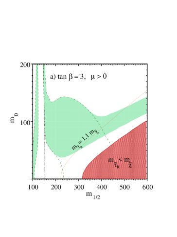
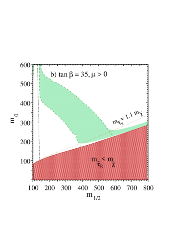
Figure 36: The light-shaded area is the cosmologically preferred region with $0.1\leq\Omega_{\chi}h^{2}\leq 0.3$, for a) $\tan\beta=3$ and b) $\tan\beta=35$. The dashed line shows the location of the cosmologically preferred region if one ignores the light sleptons. In the dark shaded regions, the LSP is the ${\tilde{\tau}}_{R}$, leading to an unacceptable abundance of charged dark matter. Also shown as a dotted line is the contour $m_{{\widetilde{\tau}}_{\scriptscriptstyle\rm R}}=1.1\,m_{\chi}$. The dot-dashed lines are contours of $m_{\chi^{\pm}}=91{\rm\,Ge\kern-1.25ptV}$.

As a first step away from the parameter restrictions of mSUGRA, one may relax the Higgs soft mass² unification constraint, so that $\mu$ and $m_{A}$ are no longer determined by the conditions of electroweak symmetry breaking. This allows for $M_{2}\gg\mu$, so that the lightest neutralino is Higgsino-like. In this case the neutralino can annihilate through $Z^{0}$ and Higgs exchange, and annihilation is typically quite efficient. Additionally, in the pure Higgsino region, the mass of the lightest neutralino is close to the masses of the next-to-lightest neutralino and lightest chargino, and the coannihilation of the LSP with the NLSP and NNLSP can play an important rôle in further reducing the neutralino relic abundance. Searches for chargino and associated neutralino production at LEP2 have already excluded the regions of parameter space where the relic density of light Higgsinos (i.e. with masses $\mathrel{\raise 1.29167pt\hbox{$<$\kern-7.5pt\lower 4.30554pt\hbox{$\sim$}}}500{\rm\,Ge\kern-1.25ptV}$) is greater than 0.3 efgos . In the pure gaugino regime $\mu\gg M_{2}$, the bounds are similar to the mSUGRA case.

As one wanders farther from the constraints of mSUGRA, the neutralino relic density will depend on new CP-violating phases in $\mu$ and $A$fos , the conditions of gaugino and scalar mass unification an ; dnry , etc., and the relic density will then have to be considered separately for each case.

XV Cold Dark Matter Searches

XV.1 Introduction

Supergravity GUT models with $R$-parity invariance possess a cold dark matter candidate: the lightest neutralino ($\chi_{1}^{0}$) 1 . Relic density calculations indicate that the predicted amount of relic $\chi_{1}^{0}$ is in accord with astronomical measurements of cold dark matter, i.e. $0.05\leq\Omega_{\chi_{1}^{0}}h^{2}\leq 0.30$, for a significant part of the SUSY parameter space for mSUGRA models. Measurements of rotation curves of a large number of spiral galaxies (including the Milky Way) indicate that their halos are composed mostly of dark matter. For the Milky Way, the local density of dark matter (DM) is estimated to be $\rho_{DM}=0.3\ GeV/cm^{3}$. (This number may be in error by a factor of two, e.g. if the halo is flattened it would be larger, while if part of the halo is baryonic machos, the SUSY component would be smaller). These dark matter particles are incident on the solar system with a velocity of $v\simeq 300\ km/s$, and hence with a flux of $\simeq 10^{5}\ (100\ GeV/m_{\chi_{1}^{0}})cm^{-2}s^{-1}$. Astronomical measurements essentially observe only the gravitational interactions of the dark matter. However, with such a flux it may be possible to observe dark matter more directly through electroweak interactions using detectors on the Earth. Techniques that have been proposed for observing neutralino DM fall into three categories:

1. Direct detection of incident $\chi_{1}^{0}$ by their scattering off quarks in a nuclear target.

2. Indirect detection of $\chi_{1}^{0}$ which accumulate in the center of the Sun or Earth and annihilate producing $\nu_{\mu}$.

3. Indirect detection from annihilation of halo $\chi_{1}^{0}$ into final states of antiprotons, positrons and gamma rays.

XV.2 Direct Detection of Dark Matter

Neutralinos may scatter off quarks via $s$-channel squark poles and $t$-channel $Z$ and Higgs poles. The effective Lagrangian that governs this interaction has the form ${\cal L}={\cal L}^{SD}+{\cal L}^{SI}$ 2 where the spin dependent (SD) part has the form

$${\cal L}^{SD}=(\bar{\chi}_{1}\gamma^{\mu}\gamma^{5}\chi_{1})[\bar{q}\gamma^{\mu}(A_{L}P_{L}+A_{R}P_{R})q]$$ (166)

($P_{L,R}={1\over 2}(1\mp\gamma^{5})$, $q(x)=$ quark field) and the spin independent (SI) part has the form

$${\cal L}^{SI}=(\bar{\chi}_{1}\chi_{1})(\bar{q}Cm_{q}q)$$ (167)

The coefficients $A_{L,R}$ come from the $Z$ pole and squark pole, while $C$ arises from the neutral $h$ and $H$ Higgs exchanges and the squark pole. Even if $m_{H}^{2}\gg m_{h}^{2}$ (as is common in mSUGRA for low and intermediate $\tan\beta$), the heavy Higgs can make a significant contribution to the $d$-quark part of $C$. The reason for this is that for $d$-quarks the $H$ contribution relative to the $h$ contribution is ($m_{h}^{2}/m_{H}^{2}\tan\alpha$) where $\alpha$ is the rotation angle that diagonalizes the $h-H$ mass matrix. For a wide range of parameters one finds (including loop corrections) $\tan\alpha=O(1/10)$ which can overcome the smallness of $m_{h}^{2}/m_{H}^{2}$. Further, for large $\tan\beta$, $m_{H}$ need not be very large. To obtain the total nuclear cross section, one must add up the scattering from each quark in a nucleon, and each nucleon in the nucleus. The SI scattering adds coherently giving a scattering amplitude proportional to $M_{N}$, the nuclear mass, while the SD scattering is incoherent. The total detector scattering event rate then has the form

$$R=[R_{SI}+R_{SD}]\biggl{[}{\rho_{\chi_{1}^{0}}\over 0.3\rm\ GeVcm^{-3}}\biggr{]}\biggl{[}{v_{\chi_{1}^{0}}\over 320\rm\ km/s}\biggr{]}\rm{events\over kg\ d}$$ (168)

where

$$R_{SI}={16m_{\chi_{1}^{0}}M_{N}^{3}M_{Z}^{4}\over[M_{N}+m_{\chi_{1}^{0}}]^{2}}|A_{SI}|^{2};\quad R_{SD}={16m_{\chi_{1}^{0}}M_{N}\over[M_{N}+m_{\chi_{1}^{0}}]^{2}}J(J+1)|A_{SD}|^{2}$$ (169)

where $A_{SI,SD}$ are the SI, SD amplitudes and $J$ is the spin of the nuclear target. We note that for $M_{N}$ large $R_{SI}\sim M_{N}$ (due to the coherent nature of SI scattering) while $R_{SD}\sim 1/M_{N}$ and so for heavy targets the spin independent scattering dominates. This is true even for relatively light nuclei unless the nucleus has very large spin interactions (e.g. $F$) and even there, $R_{SD}$ dominates only when both $R_{SD}$ and $R_{SI}$ are small. The above calculations of $R$ contain a number of uncertainties. Thus one needs to know the quark content of the nucleon and there are experimental uncertainties, particularly in the strange quark contribution. In addition, the nucleons bind in the nucleus, and assumptions about nuclear form factors must be made. Along with the uncertainty in the value of $\rho_{\chi_{1}^{0}}$ mentioned above, predictions of Eq.(168) are probably uncertain to within a factor of three. A large number of different terrestial dark matter detectors have been built or are being considered 3 . These include cryogenic detectors (with recoil and ionization signals) based on Ge, Al₂O₃, LiF, Sn, Si, superconducting granule detectors, and scintilation detectors based NaI, Xe, CaF and A. (The last type of detector has the possibility of becoming quite large with nuclear targets of 100 kg or more.)

Figure 37 shows the maximum and minimum event rates expected for a Ge detector (solid curve) for the mSUGRA model when the SUSY parameter space of $m_{0}$, $m_{\tilde{g}}\leq 1\ TeV$, $|A_{t}/m_{0}|\leq 7$, $2\leq\tan\beta\leq 25$ is scanned. One sees that event rates may vary by a factor of $10^{3}$ over this space, the high event rates coming from large $\tan\beta$ and the low rates from small $\tan\beta$. The maximum event rate curve is governed by a somewhat complex play of phenomena. Thus in the relic density analysis, the $h$ and $Z$ $s$-channel poles are a dominant contribution in the region $40\ GeV\stackrel{{\scriptstyle<}}{{\sim}}m_{\chi_{1}^{0}}\stackrel{{\scriptstyle<}}{{\sim}}55\ \rm GeV$ and this gives rise to rapid annihilation which can be compensated for by $m_{0}$ becoming large so that too much annihilation does not occur (i.e. so that $\Omega_{\chi_{1}^{0}}h^{2}\geq 0.05$). As one moves to higher $m_{\chi_{1}^{0}}$ in the relic density analysis, the $t$-channel sfermion contributions become dominant, and $m_{0}$ must remain small (i.e. $m_{0}\stackrel{{\scriptstyle<}}{{\sim}}200\rm\ GeV$) to get sufficient annihilation (i.e. so that $\Omega_{\chi_{1}^{0}}h^{2}\leq 0.3)$. The rise in the maximum event rate curve of Fig.37 as $m_{\chi_{1}^{0}}$ increases toward 60 GeV reflects this reduction in $m_{0}$, since then the squark mass is reduced and the $\chi_{1}^{0}$-quark scattering through the $s$-channel squark pole is increased. The fall off of the event rate for $m_{\chi_{1}^{0}}\stackrel{{\scriptstyle>}}{{\sim}}60\rm\ GeV$ is due to the decreasing $\chi_{1}^{0}$-quark cross section as $m_{\chi_{1}^{0}}$ increases. Current detectors hope to obtain a sensitivity of $R\geq 10^{-2}\rm\ events/kg\ d$ which will impinge on the part of the SUSY parameter space with large $\tan\beta$. The large $\tan\beta$ domain is the more difficult one for accelerator discovery of SUSY, since the tri-lepton signal is weakened due to increased $\tau$ and $b$ final state events 5 ; barkao2 . Thus dark matter searches and accelerator searches are to some extent complementary. However, the detection of soft leptons from $Z$ decays restores the trilepton search coverage of the large $\tan\beta$ regionbarkao2

Figure 37: Maximum and minimum event rates for scattering of $\chi_{1}^{0}$ by a $Ge$ target with relic density constraint $0.05\stackrel{{\scriptstyle<}}{{\sim}}\Omega_{\chi_{1}^{0}}h^{2}\stackrel{{\scriptstyle<}}{{\sim}}0.30$ without $p$ decay constraint (solid), with constraint $\tau(p\rightarrow\bar{\nu}K)>5.5\times 10^{32}yr$ (dashed and dotted) [4].

XV.3 Indirect Detection of Dark Matter

Dark matter particles in the halo of the galaxy can annihilate into ordinary matter. Three possible final state particles that might be observable are $\bar{p}$, $e^{+}$ and $\gamma$’s 1 . For the $\bar{p}$ case, the primary cosmic ray background is reduced by considering the energy region $E_{\bar{p}}\lower 3.01385pt\hbox{$\;\stackrel{{\scriptstyle\textstyle<}}{{\sim}}\;$}1\ GeV$, and it is conceivable that a signal of this type is detectable. However, there is still a considerable uncertainty concerning backgrounds. The Majorana nature of the $\chi_{1}^{0}$ prevents an annihilation into a two body $e^{+}+e^{-}$ final state, and hence, as in the $\bar{p}$ case one expects a continuum spectrum that is difficult to separate from background. However, a heavy neutralino might annihilate into a $W^{+}+W^{-}$ pair followed by $W^{+}\rightarrow e^{+}+\nu_{e}$. One expects here a peak at $E_{e^{+}}\simeq{1\over 2}m_{\chi_{1}^{0}}$ in the positron distribution. There are again background uncertainties, though this represents a possible signal for $\chi_{1}^{0}$ dark matter. The cleanest signal is the two body annihilation

$$\chi_{1}^{0}+\chi_{1}^{0}\rightarrow\gamma+\gamma;\quad E_{\gamma}\cong m_{\chi_{1}^{0}}$$ (170)

since there are no astrophysical backgrounds with discrete photon energy. Thus an observation of this process would be a clean signal for halo $\chi_{1}^{0}$ dark matter. However, since the process proceeds through a loop and is order $\alpha^{4}$, the annihilation cross section is small, and one would likely require $\rho_{\chi_{1}^{0}}$ to be a factor of 10 larger than it is currently thought to be for this process to be observable. Such large values of $\rho_{\chi_{1}^{0}}$ might possibly be true in the center of the galaxy or if dark matter clusters in the halo, though again, astrophysical uncertainties make such posibilities unclear. An alternate way of indirectly observing halo $\chi_{1}^{0}$ arises from the fact that $\chi_{1}^{0}$ incident on the sun or earth may be gravitationally captured. From subsequent scattering they will sink to the center and accumulate there. Annihilation can then occur into ordinary matter resulting in neutrinos at the end of a cascade decay chain:

$$\chi_{1}^{0}+\chi_{1}^{0}\rightarrow\nu_{\mu}+X$$ (171)

The $\nu_{\mu}$ can escape from the center of the sun or earth and be detected by terrestial neutrino telescopes. The clearest signals come from upward going muons arising from $\nu_{\mu}\rightarrow\mu$ conversion in the rock of the earth. In general, over the age of the solar system, the capture rate and annihilation rate of neutralinos come into equilibrium for the sun and in at least part of the parameter space also for the earth. Thus the number of $\nu_{\mu}$ observed will be scaled by $\rho_{\chi_{1}^{0}}$. Further, process (171) gives rise to a spectrum of $\nu_{\mu}$ with energies of about $E_{\nu_{\mu}}\approx{1\over 3}m_{\chi_{1}^{0}}$. Thus the neutrinos from $\chi_{1}^{0}$ annihilation can be distinguished from atmospheric neutrinos and other solar neutrinos. Neutrino telescopes being built are NESTOR and AMANDA with sizes of about $(10^{3}\mbox{--}10^{4})\rm\,m^{2}$ with a proposed expansion of AMANDA to $10^{6}\rm\,m^{2}\ (ICE^{3})$. For the coherent SI interactions (which are generally the largest interactions) one has roughly that a neutrino telescope of $(10^{5}\mbox{--}10^{6})\rm\,m^{2}$ corresponds to a direct Ge detector of 1 k 6 (though the neutrino telescope may become more sensitive for very large $\tan\beta$ and non-universal soft breaking 7 ). For the smaller SD interaction, a neutrino telescope of $10^{3}\rm\ m^{2}$ roughly corresponds to a 1 kg Ge detector.

XV.4 What Can Dark Matter Tell Accelerator Physics

Current accelerator searches have begun to significantly restrict the mSUGRA parameter space. Thus the $b\rightarrow s+\gamma$ branching ratio combined with the nearness of the top quark mass to the Landau pole has eliminated most of the $\mu<0$ part of the parameter space and almost all of the $A_{t}>0$ region (in ISAJET notation). Direct searches at the Tevatron imply $m_{\tilde{g}}\stackrel{{\scriptstyle>}}{{\sim}}250\ GeV$, and LEP189 data implies $m_{\chi_{1}^{\pm}}>95\rm\ GeV$. (The latter, by scaling, implies $m_{\tilde{g}}\stackrel{{\scriptstyle>}}{{\sim}}350\rm\ GeV$ for most of the allowed parameter space.) If some dark matter detector were to discover $\chi_{1}^{0}$ dark matter, it would determine at least two things: the mass of the $\chi_{1}^{0}$ (from recoil energy) and the event rate. As an example of what this might imply, the DAMA NaI experiment has recently suggested that its data may be showing a seasonal variation in event rates 8 . Assuming this effect is real, a fit to the data gave $m_{\chi_{1}^{0}}\simeq 60\rm\ GeV$. From the sensitivity of the apparatus, the mSUGRA event rate must be close to the maximum event rate curve of Fig.37, which implies that $\tan\beta$ is relatively large, i.e. $\tan\beta\approx$ 10–20. By scaling one expects then $m_{\chi_{1}^{\pm}}\simeq 100\rm\ GeV$ and $m_{\tilde{g}}\simeq 400\rm\ GeV$. Relic density constraints imply $m_{0}\stackrel{{\scriptstyle<}}{{\sim}}(150\mbox{--}200)\rm\ GeV$ in this region, implying that for the first two generations $m_{\tilde{q}}\simeq m_{\tilde{g}}$ and $m_{h}\simeq 110\rm\ GeV$. The above results imply that the $\chi_{1}^{\pm}$ may not be accessible to LEP. However, the Run IIb (with $20\rm\ fb^{-1}$ of luminosity) should be able to see the light Higgs and the $\chi_{1}^{\pm}$, while the gluino would be at the edge of observability. Further, with most of the SUSY parameters determined, most of the mSUGRA mass spectrum not accessible to the Tevatron would be predicted for the LHC. While the above NaI detector data has, of course, not been confirmed, and if dark matter is discovered in some other region of the parameter space it may be harder to extract the SUSY parameters and masses, the example illustrates the impact dark matter detection could have on accelerator physics.

XV.5 Proton decay

Grand unified models where both quarks and leptons reside in the same representation, generally give rise to proton decay. SUSY models with $R$-parity invariance forbid the dimension four operators which would yield a much too rapid proton decay, but generally allow for dimension five operators arising due to the exchange of color triplet Higgsinos, $\tilde{H}_{3}$. It is possible to suppress this operator by assuming that more than one pair of $3+\bar{3}$ color triplets exist, and with only a moderate amount of fine tuning, one can increase the lifetime by a factor of 10 in this way. Thus predictions of $p$-decay are more model dependent than other mSUGRA predictions. We consider first the mSUGRA $SU(5)$ model where there is only one pair of color triplets embedded in the $SU(5)$ $5+\bar{5}$ representations. The dominant decay mode is then usually $p\rightarrow\bar{\nu}K^{+}$ with a decay rate given by 9

$$\Gamma(p\rightarrow\bar{\nu}K^{+})=\sum_{i=,e,\mu,\tau}\Gamma(p\rightarrow\bar{\nu}_{i}K^{+})=\biggl{(}{\beta_{p}\over M_{H_{3}}}\biggr{)}^{2}|A|^{2}|B|^{2}C$$ (172)

where $M_{H_{3}}$ is the Higgs triplet mass, $\beta_{p}$ is the matrix element of the three quark operator between the vacuum and the proton state (lattice gauge calculations give $\beta_{p}=5.6\times 10^{-3}\rm\,GeV^{3}$ 10 ). $A$ is a factor depending on quark masses and CKM matrix elements, $B$ contains the dressing loop integral involving SUSY masses, and $C$ contains the chiral current algebra factors that convert quarks into mesons and baryons. There are a number of uncertainties in inputs in the above result, e.g. the value of $\beta_{p}$, CKM elements etc., and one estimates that the prediction of $(M_{H_{3}})^{2}\Gamma$ has an uncertainty of perhaps a factor of two or three. In the following we assume $M_{H_{3}}\leq 10M_{G}$. For mSUGRA $SU(5)$, the second generation contribution to Eq.(172) dominates, and one roughly finds that

$$\Gamma\approx const\biggl{(}{m_{\tilde{g}}\over m_{0}^{2}}\tan\beta\biggr{)}^{2}$$ (173)

Equation (173) shows the effects that bounds on the proton lifetime have on the SUSY parameter space, since large $m_{\tilde{g}}$, large $\tan\beta$ and small $m_{0}$ will destabilize the proton. These effects can be seen in Fig.38 where the maximum $p\rightarrow\bar{\nu}K$ lifetime is plotted vs. $m_{\tilde{g}}$ (as one scans the parameter space with $\tan\beta\leq 25$) 4 . The current data does not yet constrain the model, though Super Kamiokande will be able to test the model completely for $m_{0}\leq 1\ TeV$ (solid curve). For $m_{0}>1\ TeV$, the curves lie higher and there will still be regions not tested by Super Kamiokande.

Figure 38: Maximum $\tau(p\rightarrow\bar{\nu}K)$ for minimal $SU(5)$ mSUGRA with $m_{0}\leq 1\rm\ TeV$ (solid), $m_{0}\leq 1.5\ TeV$ (dot-dashed), $m_{0}\leq 2\ TeV$ (dashed) [4]. The solid horizontal line is the Kamiokande experimental bound, and the dashed horizontal line the expected sensitivity of Super K. [4]. The current Super K bound is $\tau_{p}>5.5\times 10^{32}yr$ at 90% C.L. [11].

Figure 39: Maximum $\tau(p\rightarrow\bar{\nu}K)$ for minimal $SU(5)$ mSUGRA with the relic density constraint $0.05\leq\Omega_{\chi_{1}^{0}}h^{2}\leq 0.30$ with $m_{0}\leq 1\rm TeV$ (dotted) and $m_{0}\leq 1.5\rm\ TeV$ (dashed), and $m_{0}\leq 2TeV$ (solid) [4]. Horizontal lines are the current and expected future Super Kamiokande bounds.

It is interesting now to combine the above results with the constraints arising from the dark matter analyses. In the relic density analysis, there are roughly two separate domains. As discussed above, for the region $m_{\tilde{g}}\stackrel{{\scriptstyle<}}{{\sim}}450\rm\ GeV$ ($m_{\chi_{1}^{0}}\stackrel{{\scriptstyle<}}{{\sim}}55\rm\ GeV$) annihilation of $\chi_{1}^{0}$ in the early universe can proceed sufficiently rapidly through $s$-channel $Z$ and $h$ poles so that $m_{0}$ can be quite large and still the relic density obeys the astronomical bounds of $0.05\leq\Omega_{\chi_{1}^{0}}h^{2}\leq 0.30$. Thus in this region, as can be seen from Eq.(173), the maximum $p$ lifetime can be quite large. In the region $m_{\tilde{g}}\stackrel{{\scriptstyle>}}{{\sim}}450\rm\ GeV$, the annihilation of $\chi_{1}^{0}$ proceeds mainly through $t$-channel sfermion poles, and to get sufficient annihilation these must be light. Here one finds that $m_{0}\stackrel{{\scriptstyle<}}{{\sim}}150\rm\ GeV$, reducing the maximum $p$ lifetime by a factor of between 10 and 30. This effect can be seen in Fig.39 where the dotted curve shows the maximum $p$ lifetime when the relic density constraint is imposed for $m_{0}\leq 1\rm\ TeV$. We see now that current $p$ decay data ($\tau_{p}>5.5\times 10^{32}\rm\,yr$ [11]) already excludes the domain $m_{\tilde{g}}\stackrel{{\scriptstyle>}}{{\sim}}350\rm\ GeV$, and even if the $m_{0}$ bound is raised to $m_{0}\leq 2TeV$ (dashed curve) the excluded region is $m_{\tilde{g}}\stackrel{{\scriptstyle>}}{{\sim}}450\rm\ GeV$. Since the current LEP189 bound of $m_{\chi_{1}^{\pm}}>95\rm\ GeV$ already excludes $m_{\tilde{g}}\stackrel{{\scriptstyle<}}{{\sim}}350\rm\ GeV$, most of the parameter space of this model has been eliminated when the relic density constraints are included. One can consider non-minimal extensions of the $SU(5)$ model. The inclusion of Yukawa textures so that the low energy limit of the theory gives rise to correct quark-lepton mass ratios raises the $p$ lifetime by a factor of about 3–5. Combined with the above mentioned uncertainty in the calculations of $\Gamma(p\rightarrow\bar{\nu}K)$ of a factor of 2–3, one might have a total increase in the theoretical curves of 5–15. The above exclusion region of $m_{\tilde{g}}\stackrel{{\scriptstyle>}}{{\sim}}450\rm\ GeV$ would then be reached when Super Kamiokande obtains a sensitivity of about $8\times 10^{32}\rm\,yr$.

The above considerations hold for other GUT groups that contain an $SU(5)$ subgroup and have matter embedded in that $SU(5)$ in the usual way. A notable exception is $SO(10)$ where $t-b$ Yukawa unification requires $\tan\beta$ to be very large, i.e. $\tan\beta=56$. From Eq.(173) one sees that this requirement will significantly reduce the $p$ lifetime. (In $SU(5)$, current data generally requires $\tan\beta<10$.) Further analyses is required to see which $SO(10)$ models with conventional proton decay will remain viable. Equation (173) shows that the maximum $p$ lifetime occurs mainly from the low $\tan\beta$ and high $m_{0}$ part of the parameter space. As discussed in Sec. XV.2, the dark matter detector event rates increase with $\tan\beta$ and decrease with $m_{0}$, the maximum event rates generally occuring at high $\tan\beta$ and low $m_{0}$. One expects, therefore, a reduction of event rates if one imposes the constraints from $p$ lifetime bounds. This can be seen in Fig.37. The dotted and dashed curves give the maximum and minimum event rates when the proton decay constraint [11] is imposed. [In the dotted curve, we have multiplied the conventional result [9] for $\tau(p\rightarrow\bar{\nu}K)$ by 20 to account for the above mentioned corrections for Yukawa textures and other uncertainities. (Note in this case the region $56{\rm\ GeV}\leq m_{\chi^{0}_{1}}\leq 67\rm\ GeV$ is forbidden.) The dashed curve multiplies the conventional result by 100 corresponding to an additional decay suppression that could arise from more than one pair of superheavy Higgs color triplets.] Proton decay in $SU(5)$-type models can always be suppressed by chosing a complicated Higgs sector. Predictions are thus model dependent. If one considers the conventional models where this tuning is not done, then the combined effects of relic density constraints and $p$ decay bounds generally imply that the gluino is relatively light i.e. $m_{\tilde{g}}\stackrel{{\scriptstyle<}}{{\sim}}\rm\ 450GeV$. The Run IIb is expected to be sensitive to gluinos with mass up to 400 GeV in direct searches, and indirectly from the discovery potential of the $\chi_{1}^{\pm}$ to gluinos of mass greater than $500\rm\ GeV$. Thus in such models gluinos will be in a range that may be accessible to the Tevatron.

XVI Charge and Colour Breaking Constraints

Vacuum stability bounds are a particularly important issue for supersymmetric models because of the large number of scalars, any of which can get a vacuum expectation value, possibly breaking charge and/or colour. Here we shall give a short discussion of these bounds concentrating on two questions;

• How do the bounds restrict the parameter space in the mSUGRA model?

• How do they restrict models with non-universal supersymmetry breaking?

XVI.1 Introduction and the mSUGRA Model

Insisting that the physical vacuum be stable results in a set of constraints on the possible supersymmetry breaking parameters which are known as Charge and Colour Breaking (CCB) bounds ccb1 ; casas1 ; baer ; as98a ; as98b ; casas2 ; af98 . There are different schools of thought regarding the precise cosmological meaning of these bounds (see for example Ref.af98 for a recent discussion). Here we take the point of view that unphysical minima lower than the physical vacuum should be avoided. There are two important kinds of bounds which result; $D$-flat directions which develop a minimum due to large trilinear supersymmetry breaking terms; $D$ and $F$ flat directions which correspond to a combination of gauge invariants involving $H_{2}$. The first kind of flat directions give a familiar set of constraints on the trilinear couplings which is typically of the form

$$A_{t}^{2}\,\raisebox{-2.58334pt}{$\buildrel<\over{\sim}$}\,3(m_{H_{U}}^{2}+m_{t_{R}}^{2}+m_{t_{L}}^{2}),$$ (174)

where the notation is conventional. These constraints turn out to be very weak. A more sophisticated treatment (in which the constraint is optimised by finding the deepest direction close to the $D$ flat direction) results in a set of ‘generalised’ CCB bounds which are much stronger casas1 . By far the most severe bounds, however, come from the directions which are $F$ and $D$ flat and we shall concentrate on these.

$F$ and $D$ flat directions develop a minimum because of the negative mass-squared term, $m_{H_{U}}^{2}$, of the Higgs which couples to the top-quark. Whilst the latter is a great success for driving electroweak symmetry breaking, it can generate an undesirable minimum radiatively. These directions are constructed from conjunctions of $L_{i}H_{2}$ plus any one of the following gauge invariants as98b ,

$$LLE\mbox{, }LQD\mbox{, }QULE\mbox{, }QUQD\mbox{, }QQQLLLE.$$ (175)

Absence of CCB minima along the first two directions is usually enough to guarantee their absence along the rest as98b . As an example consider the $L_{i}L_{3}E_{3}$, $L_{i}H_{2}$ direction, which corresponds to the choice of VEVs,

$$h_{2}^{0} = -a^{2}\mu/h_{E_{33}}$$

$$\tilde{e}_{L_{3}}=\tilde{e}_{R_{3}} = a\mu/h_{E_{33}}$$

$$\tilde{\nu}_{i} = a\sqrt{1+a^{2}}\mu/h_{E_{33}},$$ (176)

where $a$ parameterizes the distance along the flat direction. The potential along this direction is $F$ and $D$-flat and depends only on the soft supersymmetry breaking terms;

$$V=\frac{\mu^{2}}{h_{D_{33}}^{2}}a^{2}(a^{2}(m_{H_{U}}^{2}+m_{L_{ii}}^{2})+m_{L_{ii}}^{2}+m_{E_{33}}^{2}+m_{L_{33}}^{2}).$$ (177)

The first term dominates at large VEVs when $a\gg 1$ and it is this that generates the dangerous CCB minimum with a VEV which is typically a few orders of magnitude larger than the weak scale baer . There is an ‘optimum’ direction very close to this one which is slightly deeper casas1 ; baer . In order to minimise the one-loop corrections, the mass squared parameters in Eq.(177) should be evaluated at either the scale of the running top quark mass, $h_{t}H_{U}^{0}$, or at $M_{susy}$, whichever is the larger.

For a given choice of supersymmetry breaking parameters it is now straightforward to determine whether the potential has a minimum which is lower than the physical one. The results for mSUGRA are shown in Figure 40 where we plot the regions in the ($m_{0},m_{1/2}$) plane in which there are CCB minima, for three different values of $\tan\beta$ and $\mu<0$. We choose a universal trilinear coupling of $A_{0}=m_{1/2}$ for the low $\tan\beta$ diagrams, since this is the value which minimises the regions with a CCB minimum baer ; as98a ; as98b . The $\tan\beta=45$ diagram has $A_{0}=0$. The light shading denotes the cosmolgically preferred region with $0.1<\Omega_{\chi}h^{2}<0.3$, where the upper bound originates from a lower limit of 12 Gyr on the age of the universe. Thus we can see that, in mSUGRA, CCB minima when combined with dark matter constraints and experimental constraints are extremely restrictive. For example, we find that the Higgs mass lower bound, together with the cosmological constraint, implies that the mSUGRA electroweak vacuum cannot be stable for values of $\tan\beta<2.3$ for $\mu<0$. In addition, at high $\tan\beta$, large regions of parameter space become excluded by trilinear constraints and by the requirement of correct electroweak symmetry breaking.

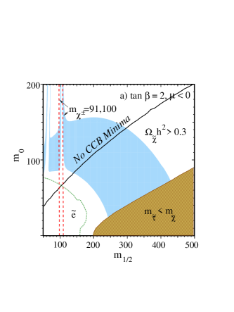
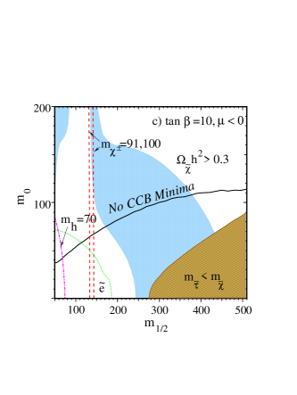
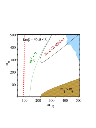
Figure 40: Experimental, dark matter and CCB Constraints on the mSUGRA model.

XVI.2 Non-universal supersymmetry breaking

Although mSUGRA continues to provide a good working model of physics beyond the Standard Model, at the time of writing there is much interest in models, derived from both perturbative and non-perturbative string theory, in which the supersymmetry breaking is non-universal. In specific cases, where there are few parameters, it is possible to continue using the numerical techniques outlined above. Indeed, recently, a variety of string derived models were shown to also suffer from severe CCB problems casas2 . For theories with a larger number of independent parameters however, it becomes increasingly difficult to pursue this option. In more general models progress can be made at low $\tan\beta$ if some accuracy is sacrificed as98a ; as98b . In Ref.as98b general expressions were derived which are valid in the one-loop approximation and in the (low $\tan\beta$) approximation that the bottom and tau Yukawas can be neglected. Defining $\tilde{m}=m/m_{1/2}$, CCB minima are absent when the following bound is satisfied.

$$\left.(2\tilde{m}_{L_{ii}}^{2}+\tilde{m}_{H_{U}}^{2}-\tilde{m}^{2}_{U_{33}}-\tilde{m}^{2}_{Q_{33}})\right|_{0}\,\raisebox{-2.58334pt}{$\buildrel>\over{\sim}$}\,f(\tilde{B}|_{0})+(\rho_{p}-1)\left(g(\tilde{B}|_{0})+3\tilde{M}^{2}|_{0}-\rho_{p}(1-{\tilde{A}_{U_{33}}}|_{0})^{2}\right),$$ (178)

where

$$\tilde{B}|_{0} = \left.(\tilde{m}_{L_{ii}}^{2}+\tilde{m}_{L_{33}}^{2}+\tilde{m}_{E_{33}}^{2})\right|_{0}$$

$$\tilde{M}|_{0} = \left.(\tilde{m}_{H_{U}}^{2}+\tilde{m}_{Q_{33}}^{2}+\tilde{m}_{U_{33}}^{2})\right|_{0}$$

$$f(x) = 1.43-0.16x+0.02x^{2}$$

$$g(x) = 2.94-0.20x+0.02x^{2}$$

$$\frac{1}{\rho_{p}} = 1+3.17(\sin^{2}\beta-\sin^{2}\beta^{QFP})$$ (179)

and where $\tan\beta^{QFP}\approx 1.6$. Note that, at the low $\tan\beta$ fixed point, the constraint is on the single combination $\left.(2\tilde{m}_{L_{ii}}^{2}+\tilde{m}_{H_{U}}^{2}-\tilde{m}^{2}_{U_{33}}-\tilde{m}^{2}_{Q_{33}})\right|_{0}$ of GUT scale parameters. In the above, $f(x)$ and $g(x)$ are fits to the bounds for $\mu=200\,{\rm GeV}$ which are accurate for $x\,\raisebox{-2.58334pt}{$\buildrel>\over{\sim}$}\,0$, and are valid for the MSSM with any pattern of supersymmetry breaking. Compared to the numerically determined bounds in mSUGRA, they are a slight overestimate at low $\tan\beta$ (by $5-10\%$) and an underestimate at higher $\tan\beta$ as the bottom quark Yukawa becomes increasingly important in the running af98 . The main inaccuracy comes from the poor determination of $\tan\beta^{QFP}$ and of course from the dependence on $\mu$ (which enters the bounds only logarithmically). For example, if we take $\mu=500\,{\rm GeV}$ we find

$$f(x)=1.20-0.14x+0.02x^{2}.$$ (180)

Although only approximate, these expressions are accurate enough to indicate whether a model is likely to suffer from severe CCB problems. For example it is found that certain versions of Horava-Witten M-theory in which supersymmetry breaking comes from bulk moduli fields (see Ref.choi and references therein) are always unstable as98b ; casas2 . Eqn.(178) also indicates that patterns of supersymmetry breaking with large slepton mass-squareds at the GUT scale are likely to be safe from CCB minima. However large slepton mass-squareds at the GUT scale also lead to large relic densities so that, in this case, the dark matter bounds and CCB bounds are negatively correlated. Note that, for the above expressions, universal gaugino masses were assumed at the GUT scale. The case of non-universal gaugino masses was examined in Ref.casas2 . In particular, in that work it was found that small $M_{3}$ and large $M_{1}$ and $M_{2}$ avoids dangerous minima. This is in accord with Eq.(178) since the renormalisation of $m_{H_{U}}^{2}$ is dominated by $M_{3}$ whereas the renormalisation of $m_{L}^{2}$ is dominated by $M_{1}$ and $M_{2}$.

Minor modifications to the superpotential of the MSSM may also lift the dangerous minimum whilst giving phenomenology which is (currently) indistinguishable from the MSSM. The simplest option is to break $R$-parity by additional (but undetectable) lepton number violating operators. Of course, in this case the constraints on $\Omega h^{2}$ no longer apply, since the LSP can decay. Alternatively, models in which electroweak symmetry breaking is driven by a singlet superfield rather than a $\mu$-parameter have a very different potential at large field values, whereas at low values they typically mimic the MSSM (see for example Ref.savoy ).

XVII $b\rightarrow s\gamma$ Constraints

An important experimental check of mSUGRA is provided by the measurement of the $b\rightarrow s\gamma$ decay rate. Weak scale SUSY particles contribute to the one loop decay amplitude, and their presence can significantly modify the Standard Model result.

The best experimental value available for the inclusive $B\rightarrow X_{s}\gamma$ branching ratio as measured by the CLEO collaboration $B(B\rightarrow X_{s}\gamma)=(3.15\pm 0.54)\times 10^{-4}$bsg-alex has to be compared to the next-to-leading order Standard Model prediction including non-perturbative corrections $B(B\rightarrow X_{s})\gamma=(3.38\pm 0.33)\times 10^{-4}$ bsg-misiak . SUSY contributions can correct the theoretical value in both directions, and a requirement that the branching ratio remain restricted within the experimental 95% confidence level band $1\times 10^{-4}<B(B\rightarrow X_{s}\gamma)<4.2\times 10^{-4}$ translates into constraints on the mSUGRA parameter space. All the next-to-leading order calculation ingredients for SUSY models are already available, with the exception of the exact two-loop matching conditions between the full theory and the effective theory. In this case, an approximate procedure effectively decoupling the heavy particles in the loop at different scales can be used for the dominating SUSY contributions bb1 .

In the MSSM, the SUSY contribution involves the charged Higgs-top quark loop, chargino-squark loops, gluino-squark loops and neutralino-squark loops hp ; masiero . The first are most important, while the gluino and neutralino loops can be safely neglected within the mSUGRA framework. The charged Higgs loop contribution is always of the same sign as the SM contribution and adds constructively with the SM loop. The chargino-squark loops, on the other hand, can interfere with the SM contribution either constructively or destructively depending on the sign of $\mu$. This feature, together with the fact that the magnitude of the total chargino-squark contribution grows with $\tan\beta$, characterizes constraints imposed on the mSUGRA parameter space by $b\rightarrow s\gamma$.

For $\tan\beta\>{\hbox{\raise 1.50696pt\hbox{$<$}}\kern-3.8889pt\kern-3.8889pt\hbox{\lower 2.79857pt\hbox{$\sim$}}}\>5$, the chargino squark contribution is small enough to permit large allowed regions for both signs of $\mu$, with larger branching ratios arising for the case of $\mu<0$. With $\tan\beta$ increasing, the allowed region in the $\mu<0$ case narrows, requiring heavy charginos to suppress $\tan\beta$ enhancement in the chargino-squark loops. In the $\mu>0$ case , cancellation between the chargino loops and the charged Higgs loop makes it possible to obtain branching ratios in some cases very close to the CLEO mean value and certainly consistent with the experimental limits over the whole range of parameters. As an example, Fig. 41 displays contours of constant branching ratio $B(b\rightarrow s\gamma)$ in the $m_{0}$ vs $m_{1/2}$ plane for $\tan\beta=2$ and $10$, and both signs of $\mu$.

In the large $\tan\beta$ parameter region with $\tan\beta\>{\hbox{\raise 1.50696pt\hbox{$>$}}\kern-3.8889pt\kern-3.8889pt\hbox{\lower 2.79857pt\hbox{$\sim$}}}\>35$, the $\mu>0$ branch of the parameter set is also constrained by $b\rightarrow s\gamma$, since a very large chargino-squark contribution drives the branching ratio below the lower experimental value of $1\times 10^{-4}$. The $\mu<0$ case requires extremely heavy superpartners ($m_{\tilde{g}}\>{\hbox{\raise 1.50696pt\hbox{$>$}}\kern-3.8889pt\kern-3.8889pt\hbox{\lower 2.79857pt\hbox{$\sim$}}}\>1500\ \rm{GeV}$, $m_{\tilde{q}}\>{\hbox{\raise 1.50696pt\hbox{$>$}}\kern-3.8889pt\kern-3.8889pt\hbox{\lower 2.79857pt\hbox{$\sim$}}}\>1600\ \rm{GeV}$) in order to satisfy experimental constraints on $B(b\rightarrow s\gamma)$ and thus imposes quite severe constraints on models with Yukawa coupling unification ltb .

Additional dependence on $A_{0}$ does not change the general picture as determined by the values of $\tan\beta$ and sign of $\mu$ but needs to be considered for a detailed analysis of mSUGRA models, since it can change the branching ratio by up to several tens of percent in either direction.

An interesting question arises in connection with CP-violating phases in SUGRA models. Traditionally, $\mu$ and $A_{0}$ have been considered to be real in all analyses concerned with $b\rightarrow s\gamma$ decay rates in this scenario. It was recently shown bsg-nath that both $\mu$ and $A_{0}$ can be complex without violating experimental limits on the neutron and electron dipole moments. Since the sign of $\mu$ plays such a crucial role in the branching ratio calculation, a completely general analysis including the complex phase of $\mu$ is necessary here to fully describe $b\rightarrow s\gamma$ constraints on the MSSM.

Figure 41: Plot of contours of constant branching ratio $B(b\rightarrow s\gamma)$ in the $m_{0}\ vs.\ m_{1/2}$ plane, where $A_{0}=0$ and $m_{t}=175$ GeV. Each contour should be multiplied by $10^{-4}$. The regions labelled by TH (EX) are excluded by theoretical (experimental) considerations. The dashed line corresponds to the LEP2 limit of $m_{\widetilde{W}_{1}}>80$ GeV for a gaugino-like chargino.

XVIII $g-2$ for Muons in an MSSM Analysis with SUGRA Induced SUSY Breaking

The anomalous magnetic moment of the muon is potentially a significant constraint for any extension of the Standard Model (SM). Currently, the measured value a_mu_exp is $a_{\mu}^{exp}\equiv\left(\frac{g_{\mu}-2}{2}\right)^{exp}=(11\,659\,230\pm 84)\times 10^{-10}$. On the other hand, the SM prediction (a_mu_th and references therein) yields $a_{\mu}^{SM}=(11\,659\,159.6\pm 6.7)\times 10^{-10}$ where the QED, electroweak and hadronic contributions are sumed and the errors are combined in quadrature. That constrains the contributions from new physics beyond the SM to fit within the

$$-70\times 10^{-10}<\delta a_{\mu}<+210\times 10^{-10}$$ (181)

window, at 90% C.L.. The width of this window is dominated by the experimental uncertainty. That, however, will change after the 1998-1999 run of the E821 experiment at BNL which is expected to reach the accuracy $\pm 10\times 10^{-10}$. If the observed central value then becomes exactly equal to the SM prediction, the new constraint will be

$$-20\times 10^{-10}<\delta a_{\mu}<+20\times 10^{-10}$$ (182)

at 90% C.L., with the window for new physics narrowed by a factor of 7.

In the MSSM, there are significant contributions from new physics due to the chargino-sneutrino and neutralino-smuon loops a_mu_MSSM . Some of these contributions are proportional to tan$\beta$. The effect can be traced back to the diagrams with the chirality flip inside the loop (or in one of the vertices) as opposed to the diagrams where the chirality flip takes place in the external muon leg. There are no similarly enhanced terms in the SM, where the chirality can only be flipped in the external muon leg. Thus for tan$\beta\gg 1$ we expect that the SUSY contribution scales versus the SM electroweak contribution $\delta a_{\mu}^{EW}$ as

$$\delta a_{\mu}^{SUSY}\simeq\delta a_{\mu}^{EW}\>\left(\frac{M_{W}}{\tilde{m}}\right)^{2}\,\tan\!\beta\simeq 15\times 10^{-10}\>\left(\frac{100{\rm GeV}}{\tilde{m}}\right)^{2}\,\tan\!\beta,$$ (183)

where $\tilde{m}$ stands for the heaviest sparticle mass in the loop (see also a_mu_MSSM ).

Our numerical analysis of the SUSY sector has been completely based on the top down approach. Three cases with low, medium, and large value of tan$\beta$ were analyzed. For low and medium tan$\beta$ ($2$ and $20$), the minimal set of the initial SUSY parameters read $M_{1/2},\;m_{0},\;A_{0},\;\mbox{\rm sign}\mu,\;\mbox{\rm and tan}\beta$, with the universal gaugino mass, scalar mass, and trilinear coupling introduced at $M_{GUT}$. The Yukawa couplings of the third generation fermions were free to vary independently on each other. For tan$\beta={\cal O}(50)$, in order to reduce severe fine-tuning required for the correct electroweak symmetry breaking, the scalar Higgs masses were allowed to deviate from $m_{0}$. The third generation yukawas at $M_{GUT}$ were strictly set equal to each other and we used the results of the global analysis of model 4c, an SO(10) model with minimal number of effective operators leading to realistic Yukawa matrices lr ; bcrw . In fact, the SO(10)-based equality $\lambda_{t}=\lambda_{b}=\lambda_{\tau}$ is the main reason why such a large tan$\beta$ is attractive. The rest of the analysis was then the same for each of the three cases. Particular values of $m_{0}$ and $M_{1/2}$ were picked up, while the rest of the initial parameters at the unification scale varied in the optimization procedure. Using the 2(1)-loop RGEs for the dimensionless (dimensionful) couplings the theory was renormalized down to low energies where the radiative electroweak symmetry breaking was checked at one loop as in bcrw and one-loop SUSY threshold corrections to fermion masses were calculated. (The latter is of particular importance for $m_{b}$ which receives significant corrections if tan$\beta$ is large.) Also, the experimental constraints imposed by the observed branching ratio $BR(b\rightarrow s\gamma)$ and by direct sparticle searches were taken into account. $\delta a_{\mu}^{SUSY}$ was evaluated for those values of the initial parameters which gave the lowest $\chi^{2}$ calculated out of the ten low energy observables $M_{Z}$, $M_{W}$, $\rho_{new}$, $\alpha_{s}(M_{Z})$, $\alpha$, $G_{\mu}$, $M_{t}$, $m_{b}(M_{b})$, $M_{\tau}$, and $BR(b\rightarrow s\gamma)$ bcrw ; br .

The results for tan$\beta=2$ and $20$ are shown in figures 43–43. The $\delta a_{\mu}^{SUSY}\times 10^{10}$ contour lines are bound from below by the limit on the neutralino mass (a limit $m_{\chi^{0}}>55$GeV was imposed), and from above by the stau mass ($m_{\tilde{\tau}}>60$GeV). The main observation is that the present limits on $\delta a_{\mu}^{SUSY}$, eq.(181) are far from excluding any region of the parameter space which is left allowed by other experiments. Note the simple pattern suggested by figures 43 and 43 shows how well the approximate relation (183) works. Overlapping the figures the contour lines marked as 10, 5, 2, 1, and 0.5 in figure 43 are roughly on top of the contour lines marked as 100, 50, 20, 10, and 5 in figure 43. The pattern seems to indicate that for tan$\beta=50$ even the present data (eq.(181)) already start constraining the MSSM analysis.

The analysis of the case tan$\beta\approx 50$ is qualitatively different. The global analysis yields two distinct fits br , see figs. 45a–b, which differ by the sign of the Wilson coefficient $C_{7}^{MSSM}$. ($C_{7}$ determines the $b\rightarrow s\gamma$ decay amplitude.) In this regime, the sign of $C_{7}$ can be the same, or the opposite, as in the SM, due to the fact that the chargino contribution is enhanced by tan$\beta$ compared to the SM. (Thus, the flipped sign of $C_{7}$ cannot be obtained for low tan$\beta$.) For large tan$\beta$ however, the fit with the flipped sign is equally good as the fit with the sign unchanged, see figure 45. Neglecting the fine-tuning issue, they just differ in the range of the allowed parameter space br . This difference then affects $\delta a_{\mu}^{SUSY}$ which is more significant in the fit with the flipped sign of $C_{7}^{MSSM}$ than in the fit where the signs are the same, see figs. 45a and 45b. The most important lesson is that the MSSM contribution to the muon anomalous magnetic moment again stays within the currently allowed range, eq.(181), assuming all other particle physics constraints are taken into account — in contradiction to the naive extrapolation from figures 43-43. This is mainly because the allowed SUSY parameter range is further reduced for large tan$\beta$ by strong constraints on the $b$ quark mass and the branching ratio $BR(b\rightarrow s\gamma)$. For $\mu>0$, the chargino contribution to $C_{7}$ changes sign too, which leads to unacceptable values of $BR(b\rightarrow s\gamma)$ for medium and large tan$\beta$. For low tan$\beta$, $\delta a_{\mu}^{SUSY}$ is small and will be hard to observe, regardless of the sign of $\mu$ a_mu_MSSM .

The E821 BNL experiment, however, turns the muon anomalous magnetic moment into a powerful MSSM constraint. Figures 43, 43, and 45 show that it will be a major constraint for large and medium tan$\beta$ in the region $m_{0}<400-500$GeV. Of course, it may drastically affect the MSSM analysis with any value of tan$\beta$ if the observed central value turns out to be below (or well above) the SM prediction. For such an outcome, the muon anomalous magnetic moment will actually become a dominant constraint for the MSSM analysis with universal SUGRA mediated SUSY breaking terms.

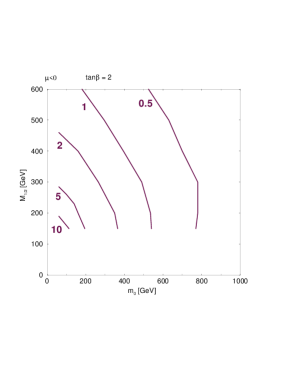
Figure 42: Contour lines of constant $\delta a_{\mu}^{SUSY}\times 10^{10}$ in the MSSM analysis with fixed tan$\beta=2$.

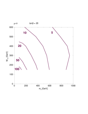
Figure 43: Contour lines of constant $\delta a_{\mu}^{SUSY}\times 10^{10}$ in the MSSM analysis with fixed tan$\beta=20$.

Figure 44: Best fit $\chi^{2}$ contour plots in the SO(10) model analysis, with the Wilson coefficient $C_{7}^{MSSM}$ of (a) the same (b) the opposite sign as compared to $C_{7}^{SM}$. As indicated, the contour lines correspond to $\chi^{2}=6,\,3$, and $0.3$ per $3\;d.o.f.$, respectively. tan$\beta$ varies between 50 and 55.

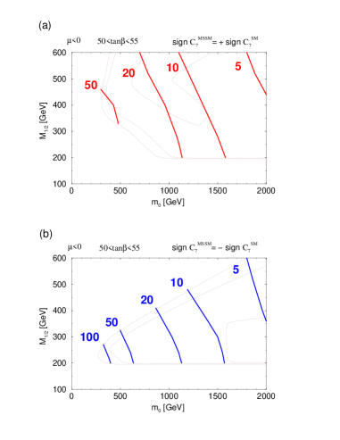
Figure 45: Contour lines of constant $\delta a_{\mu}^{SUSY}\times 10^{10}$ in the SO(10) model analysis, with the Wilson coefficient $C_{7}^{MSSM}$ of (a) the same (b) the opposite sign as compared to $C_{7}^{SM}$. For better reference, the $\chi^{2}$ contour lines of figures 45a and 45b are shown in the background of (a) and (b), respectively, as dotted lines.

XIX Effects of CP-violating Phases

In the minimal supergravity model, all parameters are assumed to be real and no CP-violating effects can originate in the superpartner sector of the Lagrangian. Once this assumption is relaxed, $m_{1/2}$, $A_{0}$ and $\mu$ can become complex, while $\tan\beta$ is still set to be real by a convenient redefinition of the Higgs fields in order to prevent spontaneous CP violation. On the other hand, R-symmetry relates the phases of the parameters and only two of the phases are physically independent. Usually, $\varphi_{\mu_{0}}$ and $\varphi_{A_{0}}$ are chosen to supplement the set of GUT scale parameters defining a non-minimal SUGRA model.

It is important to realize that $\varphi_{\mu}$ does not run as parameters are evolved from the GUT scale down to the electroweak scale while the phase of $A$ does run and is strongly affected by the magnitude of the gaugino mass terms in the RGE’s for $A$. The effect of the $\varphi_{A}$ phases increases with increasing values of $A_{0}$. Furthermore, the effects of $\varphi_{A}$ enter through the L-R off-diagonal mixing term in the squark and slepton mass matrix $m_{f}(A_{f}e^{-i\varphi_{A_{f}}}-\mu e^{i\varphi_{\mu}}f(\beta))$, where $f(\beta))=\tan\beta$ (or $\cot\beta$) for $T_{3}=-1/2$ ($+1/2$). This means that the phase of $A$ will be irrelevant if $|A_{f}|\ll|\mu|f(\beta)$.

Experimental upper limits for electron and neutron electric dipole moments impose severe constraints on the values of $\varphi_{A_{0}}$ and $\varphi_{\mu_{0}}$ if they are considered separately, requiring, e.g., $\varphi_{\mu_{0}}\lower 3.01385pt\hbox{$\;\stackrel{{\scriptstyle\textstyle<}}{{\sim}}\;$}0.01$ for $m_{1/2}\lower 3.01385pt\hbox{$\;\stackrel{{\scriptstyle\textstyle<}}{{\sim}}\;$}1$ TeV. Recently, it has been pointed out nath that cancellations between different contributions to the electric dipole moments can permit large values of these phases. As an example of the effect of cancellations between various contributions to the neutron and electron EDMs, Fig. 46 displays for $\tan\beta=2,A_{0}=1000{\rm\,Ge\kern-1.25ptV}$ the minimum value of $m_{1\!/2}$ in mSUGRA required to bring both the neutron and electron EDMs below their experimental limits (there is an identical region with $\varphi_{A}\rightarrow-\varphi_{A},\varphi_{\mu}\rightarrow-\varphi_{\mu}$) olive . The cancellations persist for a limited range in $m_{1\!/2}$, particularly at larger $\varphi_{\mu}$, and the allowed regions are between 20 and $40{\rm\,Ge\kern-1.25ptV}$ wide in $m_{1\!/2}$ for $\varphi_{\mu}/\pi>0.14$. Larger values of $A_{0}$ permit larger $\varphi_{\mu}$, but for a smaller range in $m_{1\!/2}$, while smaller $A_{0}$ requires smaller $\varphi_{\mu}$. Note that $\varphi_{\mu_{0}}>0.17\pi$ in this example would require a heavy sparticle spectrum. The maximum $\varphi_{\mu}$ scales roughly like $1/\tan\beta$. The maximum value of $\varphi_{A_{0}}$ is virtually unrestricted even for relatively light spectra in the sense that for any value of $\varphi_{A_{0}}$ there exists such a value of $\varphi_{\mu_{0}}$ and a range of $m_{1/2}$ as above so that the electric dipole moment constraints are satisfied.

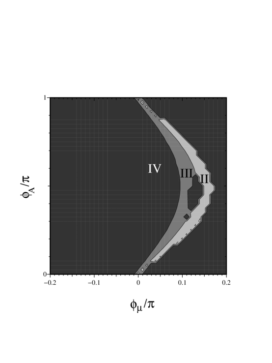
Figure 46: Plot of the required values of $m_{1\!/2}$ to satisfy the electron and neutron EDM constraints for $\tan\beta=2,A_{0}=1000{\rm\,Ge\kern-1.25ptV}$. The zones labelled “II”, “III”, and “IV” correspond to $200{\rm\,Ge\kern-1.25ptV}<m_{1\!/2}^{\rm min}<300{\rm\,Ge\kern-1.25ptV}$, $300{\rm\,Ge\kern-1.25ptV}<m_{1\!/2}^{\rm min}<450{\rm\,Ge\kern-1.25ptV}$, and $m_{1\!/2}^{\rm min}>450{\rm\,Ge\kern-1.25ptV}$, respectively.

The implications of the phases are significant from the point of view of reconstructing the parameters of the Lagrangian from experimental data cp-bk . For instance, in the chargino sector the presence of phases makes it impossible to correctly determine all parameters just by measuring the chargino masses and production cross sections as the number of parameters exceeds the number of observables. For this to be possible a measurement at an $e^{+}e^{-}$ collider with a polarized beam would be necessary. Also the Higgs sector is affected by the phases and the mass of the light Higgs as well as its production cross section can vary substantially with the variation of the phases.

Another important issue is the impact of the phases on the lightest neutralino relic density and direct detection rates cp-bk ; gor . The annihilation cross section of the lightest neutralino depends on $\varphi_{\mu}$ and as a result the relic density depends on the allowed range of $\varphi_{\mu}$. Although the lightest neutralino in SUGRA is an almost pure bino, the Higgsino admixture is very important for the direct detection rate calculation since the heavy Higgs exchange contribution dominates the scalar cross section. The rate can then vary even by a factor of two or more within the SUGRA models depending on the value of $\varphi_{\mu}$.

Minimal SUGRA is a model with a simplifying set of assumptions, and when one steps away from those assumptions, by relaxing the sfermion mass constraints, for example, or by including complex phases, some of the analyses will change (see for example cgss , for an analysis of the effect of phases on the trilepton signature). Therefore one should cautiously interpret simulations, efficiencies or analyses of data based on that model, until we know that its assumptions are confirmed experimentally. It should be noted here that when all the phases are included in the analysis of the electric dipole moment limits, none of them are required to be small bgk , so they should all be measured once there is data.

XX Flavor Violation

If the soft squark and slepton masses are non-universal, then in general they do not have to be diagonal in the same basis as the quark and lepton mass matrices. In that case, they can induce flavor-changing effects. The low energy flavor-changing processes, such as $K-\bar{K}$ mixing, $\mu\rightarrow e\gamma$, provide some probes and constraints on the non-degeneracies and mixings among different generation sfermions. On the other hand, the flavor-changing effects can also show up when the sfermions are directly produced. The superGIM mechanism suppresses the flavor-changing effects only when $\Delta m\lower 3.01385pt\hbox{$\;\stackrel{{\scriptstyle\textstyle<}}{{\sim}}\;$}\Gamma$ for real sfermions, where $\Delta m$ is the mass difference between sfermions of different generations and $\Gamma$ is the decay width of the sfermions, in constrast with $\Delta m<m$ for virtual sfermions in the low energy processesACFH . Therefore, for $\Gamma\lower 3.01385pt\hbox{$\;\stackrel{{\scriptstyle\textstyle<}}{{\sim}}\;$}\Delta m\ll m$, direct production could be a powerful probe of the flavor mixings in the sfermion sector.

However, detecting squark flavor mixings is difficult because it is hard to disentangle them from the quark flavor mixings which are already present in the Standard Model. In addition, only heavy quarks can be tagged. On the other hand, lepton flavor is conserved in the Standard Model in the absence of neutrino masses. Even in the presence of neutrino masses and mixings, the induced flavor-violating effects for the charged leptons in the rare decay processes or at colliders are too small to be observed, due to the tiny neutrino masses. Therefore, any observed lepton flavor violation in these processes implies new flavor-violating physics beyond the Standard Model.

Lepton flavor violation from slepton oscillations at lepton colliders have been studied in Ref. ACFH ; LFV . It is found that the direct slepton production often provides a more powerful probe than low energy processes, such as $\mu\rightarrow e\gamma$, in the $\Delta m-\sin 2\theta$ plane. The mixing angle $\sin\theta$ between sfermions of different generations can be probed down to $10^{-1}-10^{-2}$, which is quite interesting in comparison with the CKM matrix elements.

At the upgraded Tevatron, the sleptons are predominantly pair produced through Drell-Yan processes, mediated by a $W,\;\gamma,$ or $Z$ in the $s$-channel. The production cross sections and the possibility of detection were studied in Ref. BCPT ; BHR . The conclusion is that the detection of sleptons at the Tevatron is very difficult, unless sleptons are very light. As a result, for lepton flavor violation to have any chance to be observed at the Tevatron, sleptons must be light and have very large mixings among them.

To get a more quantitative idea of the reach at the upgraded Tevatron, we consider the following MSSM parameters, $m_{\tilde{l}_{R}}=100$ GeV, $m_{\tilde{l}_{L}}=110$ GeV, $M_{1}=60$ GeV, $M_{2}=120$ GeV, $\mu=-300$ GeV, $\tan\beta=2(30)$; these parameters do not satisfy the minimal supergravity boundary condition. Lighter sleptons can be produced at LEP II, which will do a better job in probing lepton flavor violation anyway. For heavier sleptons, the cross section will be too small for the sleptons to be observed. For this choice of parameters, both left and right handed sleptons decay directly to (lepton+LSP), so the signal for slepton production is $l\bar{l}\not\!\!E_{T}$. If two leptons are of different flavors, it is a signal for flavor violation. If the chargino decay channels for the left handed sleptons are open, the branching fractions of the signal will be reduced. The major background to the dilepton signature comes from $W$ pair production. Other backgrounds from $t\bar{t}$ production, from $Z\rightarrow\tau\bar{\tau}$, and from SUSY processes such as chargino pair production are also calculated in Ref. BCPT , and they are much smaller. The two leptons are required to be energetic and isolated to veto the Standard Model backgrounds from $W$ pair, $\tau\bar{\tau}$, and top quark pair production. The cuts imposed in Ref. BCPT are $p_{T}(l)>15$ GeV, missing tranverse energy $\not\!\!E_{T}>20$ GeV, no jet, and transverse opening angle $30^{\circ}<\Delta\phi(l\bar{l})\leq 150^{\circ}$. From Ref. BCPT , including the next-to-leading (NLO) order QCD correctionsBHR , the production cross sections for a single generation of charged sleptons in the flavor-conserving case are $\sigma_{0L}(\tilde{e}_{L}\tilde{e}_{L})\sim 21$ fb, $\sigma_{0R}(\tilde{e}_{R}\tilde{e}_{R})\sim 14$ fb, for the above slepton mass parameters. The major background from $W$ pair production is about $\sigma_{B}\sim 47$ fb (including NLO QCD corrections) after cuts. For a total integrated luminosity $L=\int{\cal L}dt$ and signal efficiency $\epsilon$, the $3\sigma$ significance requires

$$\sigma(\tilde{l}\tilde{l}^{\prime})>\frac{3}{\epsilon}\sqrt{\frac{\sigma_{B}}{L}}\approx 14\left(\frac{30\%}{\epsilon}\right)\sqrt{\frac{25{\rm fb}^{-1}}{L}}{\rm fb}.$$ (184)

In Figures 47 and 48 we plot the contours of constant ratios of flavor-violating slepton production cross sections $\sigma_{L(R)}(\tilde{e}_{L(R)}^{\pm}\tilde{\mu}_{L(R)}^{\mp})$ to $\sigma_{0L(R)}$ (we assume 2 generation mixing for simplicity) in the $\sin 2\theta_{L(R)}-\Delta m_{\tilde{l}_{L(R)}}$ plane. The $3\sigma$ contours for $\epsilon=30\%$ and $L=25\mbox{ fb}^{-1}$ are also shown. In addition, we superimpose the current constraint of $B(\mu\rightarrow e\gamma)<4.9\times 10^{-11}$ for $\tan\beta=2$ (dashed line) and 30 (dotted line). The areas above these lines are ruled out. We can see that even for an integrated luminosity as high as $L=25\mbox{ fb}^{-1}$, lepton flavor violation be observed only for a limit range of $\Delta m$ in small $\tan\beta$ and nearly maximal mixing. Therefore, we conclude that probing SUSY flavor violation is not very promising at the upgraded Tevatron. However, if flavor violation is seen at the upgraded Tevatron, it will point to a very specific and interesting region of the parameter space.

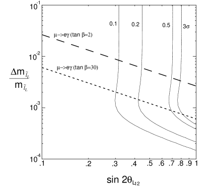
Figure 47: The constant contours of the ratio of the flavor-violating slepton production cross section $\sigma_{L}(\tilde{e}_{L}^{\pm}\tilde{\mu}_{L}^{\mp})$ to $\sigma_{0L}$, The MSSM parameters are chosen to be $m_{\tilde{l}_{R}}=100$ GeV, $m_{\tilde{l}_{L}}=110$ GeV, $M_{1}=60$ GeV, $M_{2}=120$ GeV, $\mu=-300$ GeV, $\tan\beta=2(30)$. The $3\sigma$ contour assumes the integrated luminosity $L=25{\rm fb}^{-1}$ and signal efficiency $\epsilon=30\%$. The current constraints from $B(\mu\rightarrow e\gamma)$ for $\tan\beta=2$ and $30$ are also shown; the regions above the dashed lines are ruled out.

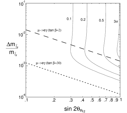
Figure 48: Same as Figure 47, except for right handed sleptons.

XXI 3rd Generation Scalar Quarks and Electric Dipole Moments in Supersymmetric Theories

CP violation in the trilinear couplings of the Higgs bosons to the scalar-top or the scalar-bottom quarks may lead to large loop effects of CP noninvariance in the Higgs sector of the minimal supersymmetric standard model (MSSM). These third-generation Yukawa couplings may directly be constrained by electric dipole moments induced by two-loop Barr-Zee-type graphs. Our analysis shows that large $\tan\beta$ scenarios with $\tan\beta>40$, $\mu,A>0.5$ TeV and large CP-odd phases are highly disfavoured.

Supersymmetric (SUSY) theories including the MSSM GD ; NS generally require some degree of fine tuning in order to account for the small flavour-changing neutral currents (FCNC) involving the first two families of quarks, and the absence of any electric dipole moment (EDM) of the neutron and electron BS . Presently, the experimental limits on the neutron EDM $d_{n}$ and electron EDM $d_{e}$ are very stringent PDG , i.e. $|d_{n}|<10^{-25}\ e$cm and $|d_{e}|<10^{-26}\ e$cm. Therefore, solutions to the CP and FCNC problems are mainly based on suppressing the contributions of the first two families of scalar quarks without affecting much the paramater space of the third generation.

In addition to the usual CP-odd phase in the Cabbibo-Kobayashi-Maskawa (CKM) matrix and the strong QCD phase $\theta$, the MSSM supplemented by the universality condition at a unification scale predicts two new CP-violating phases EFN . Specifically, two of the four complex parameters $\{\mu,\ B,\ m_{\lambda},\ A\}$ are field-independent, where $\mu$ is the mixing parameter of the two Higgs chiral superfields in the superpotential, $B\mu$ is the soft bilinear Higgs-mixing mass, $m_{\lambda}$ represents the gaugino mass, and $A_{f}=A$ is the universal soft trilinear coupling of the Higgs fields to the scalar fermions $\tilde{f}$. These can be chosen to be $\mu$ and $A$. In such a weak basis, a qualitative estimate of the combined effect of all one-loop contributions to the electron and $u$-, $d$- quark EDMs may be given by EFN ; KO ; FOS ; IN

$$\Big{(}\frac{d_{f}}{e}\Big{)}^{\rm 1-loop}\ \sim\ 10^{-25}\ {\rm cm}\times\frac{\{{\rm Im}\ \mu,\ {\rm Im}\ A_{f}\}}{\max(M_{\tilde{f}},m_{\lambda})}\ \Big{(}\,\frac{1\ {\rm TeV}}{\max(M_{\tilde{f}},m_{\lambda})}\,\Big{)}^{2}\Big{(}\,\frac{m_{f}}{10\ {\rm MeV}}\,\Big{)}\ .$$ (185)

Eq. (185) leads to the known conclusion KO that in the MSSM, large CP-violating phases are only possible if scalar quarks of the first two families or gauginos have masses in the TeV range. However, there is also another interesting scheme to suppress the one-loop EDM contributions and have most of the SUSY particles much below the TeV scale. One may require that ${\rm arg}(\mu)\stackrel{{\scriptstyle\displaystyle<}}{{\sim}}10^{-2}$, which is also favoured by dark-matter constraints FOS , and assume an hierarchic pattern for $A_{f}$’s, e.g., $[A]={\rm diag}(\epsilon,\epsilon,1)A$ with $\epsilon\stackrel{{\scriptstyle\displaystyle<}}{{\sim}}10^{-3}\,\mu/A$ CKP . In this scheme, $A_{\tau}=A_{t}=A_{b}=A$ are the only large trilinear couplings in the theory with CP-violating phases of order unity. We should note that there is also a significant three-loop contribution to neutron EDM through Weinberg’s three-gluon operator cp-SW ; DDLPD . However, these effects scale as $1/m_{\tilde{g}}^{3}$ and are therefore well below the experimental neutron EDM bound if gluinos are heavier than about 400 GeV IN . Allowing for large CP-violating trilinear couplings of the Higgs bosons to the scalar-top and scalar-bottom quarks is a rather interesting phenomenological scenario, since such Yukawa couplings can lead by themselves to large loop effects of CP noninvariance in the Higgs sector of the MSSM. More details may be found in APLB .

Most recently, we have found CKP that CP-violating Yukawa couplings involving the third generation of scalar quarks can also give rise to EDMs of electron and neutron at the observable level by virtue of the two-loop Barr-Zee-type graphs BZ ; CKY shown in Fig. 49. The two-loop EDM effects are rather enhanced in the large $\tan\beta$ regime. However, we should stress that apart from the MSSM, these novel EDM contributions are present in any supersymmetric theory. In particular, even if the first two families of scalar quarks are arranged so as to give small effects on EDMs, the two-loop Barr-Zee-type graphs may even dominate by several orders of magnitude over all other one-, two- and three-loop contributions discussed extensively in the existing literature EFN ; KO ; FOS ; IN ; DDLPD ; TKNO . The SUSY scenario we have in mind contains a large CP-violating phase in the third family $A_{\tau}=A_{t}=A_{b}=A$, and CP violation is induced through the interaction Lagrangian having the generic form

$${\cal L}_{\rm CP}\ =\ -\,\xi_{f}v\,a\,(\tilde{f}_{1}^{*}\tilde{f}_{1}\,-\,\tilde{f}_{2}^{*}\tilde{f}_{2})\ +\ \frac{ig_{w}m_{f}}{2M_{W}}\,R_{f}\,a\,\bar{f}\gamma_{5}f\,,$$ (186)

where $A$ is the would-be CP-odd Higgs boson, $M_{W}={1\over 2}g_{w}v$ is the $W$-boson mass, $\tilde{f}_{1,2}$ are the two mass-eigenstates of scalar quarks of third family, $R_{b}=\tan\beta$, $R_{t}=\cot\beta$, and $\xi_{f}$ is a model-dependent CP-violating parameter. In the MSSM, only $\tilde{t}$ and $\tilde{b}$ are expected to give the largest contributions, as the these quantities $\xi_{t}$ and $\xi_{b}$ are Yukawa-coupling enhanced, viz. APLB

$$\xi_{t}\ =\ \frac{\sin 2\theta_{t}m_{t}{\rm Im}(\mu e^{i\delta_{t}})}{\sin^{2}\beta\ v^{2}}\,,\qquad\xi_{b}\ =\ \frac{\sin 2\theta_{b}m_{b}{\rm Im}(A_{b}e^{-i\delta_{b}})}{\sin\beta\,\cos\beta\,v^{2}}\,,$$ (187)

where $\delta_{q}={\rm arg}(A_{q}+R_{q}\mu^{*})$, and $\theta_{t}$, $\theta_{b}$ are the mixing angles between weak and mass eigenstates of $\tilde{t}$ and $\tilde{b}$, respectively.

Figure 49: Two-loop contribution to EDM and CEDM in supersymmetric theories (mirror graphs are not displayed.)

In the calculation of the $\tilde{t}$- and $\tilde{b}$-mediated two-loop graphs shown in Fig. 49, we have neglected subdominant contributions emanating from analogous Barr-Zee-type graphs where the photon is replaced by a $Z$ boson, since the vectorial part of the $Z$-boson-mediated interaction is suppressed relative to the photonic one by a factor $(1-4\sin^{2}\theta_{w})/4\approx 2.4\ 10^{-2}$ with $\cos\theta_{w}=M_{W}/M_{Z}$ for the electron case, and is smaller by a factor $1/4$ for the $u$ and $d$ quarks. Taking the above into consideration, we calculate the EDM of a light fermion $f$

$$\left(\frac{d_{f}}{e}\right)^{\tilde{q}}_{\rm EW}\ =\ Q_{f}\,\frac{3\alpha_{\rm em}}{32\pi^{3}}\,\frac{R_{f}\,m_{f}}{M^{2}_{a}}\sum_{q=t,b}\ \xi_{q}\,Q^{2}_{q}\,\left[\,F\left({M^{2}_{\tilde{q}_{1}}\over M^{2}_{a}}\right)-F\left({M^{2}_{\tilde{q}_{2}}\over M^{2}_{a}}\right)\right]\,,$$ (188)

where $\alpha_{\rm em}=e^{2}/(4\pi)$ is the electromagnetic fine structure constant and all kinematic parameters are evaluated at the electroweak (EW) scale. In Eq.  (188), $F(z)$ is a two-loop function given by

$$F(z)\ =\ \int_{0}^{1}dx\ \frac{x(1-x)}{z-x(1-x)}\ \ln\Big{[}\,\frac{x(1-x)}{z}\,\Big{]}\ ,$$ (189)

which may also be expressed in terms of dilogarithmic functions CKP ; $F(z\ll 1)=\ln z+2$; $F(z\gg 1)=-{1\over 6}(\ln z+{5\over 3})/z$. Furthermore, the two-loop Barr-Zee type graphs depicted in Fig. 49 also give rise to $u$- and $d$- chromo-EDMs, i.e.,

$$\left(\frac{d^{C}_{f}}{g_{s}}\right)^{\tilde{q}}_{\rm EW}=\ \frac{\alpha_{s}}{64\pi^{3}}\,\frac{R_{f}\,m_{f}}{M^{2}_{a}}\ \sum_{q=t,b}\ \xi_{q}\,\left[F\left({M^{2}_{\tilde{q}_{1}}\over M^{2}_{a}}\right)-F\left({M^{2}_{\tilde{q}_{2}}\over M^{2}_{a}}\right)\right]\,.$$ (190)

Using the valence quark model, we can now estimate the neutron EDM $d_{n}$ induced by $d_{u}$ and $d_{d}$ at the hadronic scale $\Lambda$ including QCD renormalization effects CKY . The neutron EDM is given by

$$\frac{d_{n}}{e}\ \approx\ \left(\frac{g_{s}(M_{Z})}{g_{s}(\Lambda)}\right)^{32\over 23}\left[\,\frac{4}{3}\,\left(\frac{d_{d}}{e}\right)_{\Lambda}-\frac{1}{3}\,\left(\frac{d_{u}}{e}\right)_{\Lambda}\,\right]\,.$$ (191)

Note that in Eq. (191), all the anomalous dimension factors are explicitly separated out from quantities $(d_{d}/e)_{\Lambda}$ and $(d_{u}/e)_{\Lambda}$ which are simply given by Eq. (188) with the running couplings and the running masses of $u$- and $d$-quarks evaluated at the low-energy hadronic scale $\Lambda$. We take $m_{u}(\Lambda)=7$ MeV, $m_{d}(\Lambda)=10$ MeV, $\alpha_{s}(M_{Z})=0.12$, and $g_{s}(\Lambda)/(4\pi)=1/\sqrt{6}$ cp-SW . Likewise, the light-quark CEDMs $d_{u}^{C}$ and $d^{C}_{d}$ give rise to a neutron EDM

$$\frac{d^{C}_{n}}{e}\ \approx\ \left(\frac{g_{s}(M_{Z})}{g_{s}(\Lambda)}\right)^{74\over 23}\left[\,\frac{4}{9}\left(\frac{d^{C}_{d}}{g_{s}}\right)_{\Lambda}+\frac{2}{9}\left(\frac{d^{C}_{u}}{g_{s}}\right)_{\Lambda}\,\right]\,,$$ (192)

where quantities in the last bracket are given by Eq. (190) with the strong coupling constant $g_{s}$ and the $u$- and $d$-quark masses evaluated at the scale $\Lambda$.

Figure 50 shows the dependence of the EDMs $d_{e}$ (solid line), $d^{C}_{n}$ (dashed line), and $d_{n}$ (dotted line) on $\tan\beta$ and $\mu$, for three different masses of the would-be CP-odd Higgs boson $A$, $M_{A}=100,300,500$ GeV. Since the coupling of the $a$ boson to the down-family fermions such as the electron and $d$ quark depends significantly on $\tan\beta$, we find a substantial increase of $d_{n}$ and $d_{e}$ in the large $\tan\beta$ domain (see Fig. 50(a)). As can be seen from Fig. 50(b), EDMs also depend on $\mu$ through the $a\tilde{f}^{*}\tilde{f}$ coupling in Eq.  (186). From our numerical analysis, we can exclude large $\tan\beta$ scenarios, i.e., $40<\tan\beta<60$ with $\mu,\ A>0.5$ TeV, $M_{a}\leq 0.5$ TeV, and large CP phases. Nevertheless, the situation is different for low $\tan\beta$ scenarios, e.g.  $\tan\beta\stackrel{{\scriptstyle\displaystyle<}}{{\sim}}20$, where the two-loop Barr-Zee-type contribution to EDMs is not very restrictive for natural values of parameters in the MSSM. Finally, EDMs display a mild linear dependence on the mass of the $a$ boson for the range of physical interest, $0.1<M_{a}\stackrel{{\scriptstyle\displaystyle<}}{{\sim}}1$ TeV.

Figure 50: Numerical estimates of EDMs. Lines of the same type from the upper to the lower one correspond to $M_{a}=100,\ 300,\ 500$ GeV, respectively.

In summary, we have found that the SUSY version of the two-loop Barr-Zee mechanism (see also Fig. 49) induces observable effects on the EDMs of electron and neutron. In this way, we were able to put strict limits on the CP-violating parameters related to the third generation scalar quarks; especially the limits become very significant for large $\tan\beta$ scenarios CKP . Obviously, these novel constraints will have an important impact on possible effects of CP violation at collider and other low-energy observables, on dark-matter detection rates and searches, and on baryogenesis in SUSY theories.

XXII Run II Parameters

The Tevatron is currently being upgraded to provide a peak luminosity of $2\times 10^{32}$ cm^-2s^-1 (from $2\times 10^{31}$ cm^-2s^-1 in Run I) at $\sqrt{s}$ = 2 TeV (from 1.8 TeV). The next run, called Run II, is expected to start in 2000 and to accumulate 2 fb^-1 of data.

Both CDF cdf2_tdr and DØ d02_tdr detectors are also being upgraded for Run II, and will be are capable of operating under Run II conditions. A major upgraded detector subsystem is the tracking system, including a silicon microstrip chamber and outer tracker. In CDF, the outer tracker is a remake of the Run I drift chamber, but adapted to the more demanding conditions of Run II. In DØ, the tracker is based on a new tracking technique using scintillation fibers with a 2 T solenoidal magnet. Another key element of the CDF and DØ upgrades is their sophisticated trigger systems for much higher interaction rate in Run II. Parameters related to identification of particles at both detectors are briefly summarized in Table 11. It should be noted that:

• The $\eta$ coverage for leptons is such that we can determine the momentum of a track (and, its charge). For instance, the CDF detector can identify the electron candidate down to $\eta\approx 3$ if the momentum measurement is not required. The coverage of the lepton trigger is determined by the available hardware trigger.

• The secondary vertex trigger is available in Run II. Here, the trigger efficiency is assumed to be the same as the efficiency of the offline analysis.

• Identification (ID) of a charm quark jet is based on a technique called jet probability, which reconstructs a probability that the ensemble of tracks in a jet is consistent with being from the primary vertex. We assume the ID efficiency in Run II is the same as in Run I.

Table 11: Summary of CDF and DØ parameters for particle identification (ID) expected in Run II. The number in each parenthesis is the $\eta$ coverage for a trigger leg.

		CDF-II		DØ-II		Comments
$|\eta|$ coverage
	$\gamma$	$<2.0$	($<1.1$)	$<1.5$	($<1.5$)
	$e$	$<2.0$	($<1.1$)	$<3.0$	($<1.5$)
	$\mu$	$<2.0$	($<1.1$)	$<2.0$	($<1.7$)
	$\tau$	$<2.0$	($<1.1$)	$<2.0$	($<1.7$)
	$j$	$<3.0$		$<3.0$
	$b$	$<2.0$		$<2.0$
	$c$	$<2.0$		$<2.0$
Efficiency (%)
	$b$ ID	50%		50%		for $t\overline{t}$
	$c$ ID	50%		50%
	$\tau$ ID	40%		40%		for $W\rightarrow\tau\nu$

XXIII Review of Previous Studies on Accessible Regions and an Estimation of What Needs to be Calculated

Squarks and gluinos, if kinematically acessible, should be copiously produced in hadronic collisions. Once produced, these rapidly decay into primary jets and charginos and neutralinos. The charginos and neutralinos further decay until the cascade terminates in the lightest neutralino, which we assume is the LSP. Events with hard jets (from the primary decay) together with $E\hbox to0.0pt{\hss/}_{T}$ from the escaping LSPs, and possibly leptons, from the secondary decays of charginos and neutralinos would signal gluino and/or squark production at the Tevatron. If squarks and gluinos are too heavy to be produced at the Tevatron, the reactions $p\bar{p}\rightarrow\tilde{\chi}^{\pm}_{1}\tilde{\chi}^{0}_{2}$, and $p\bar{p}\rightarrow\tilde{\chi}^{\pm}_{1}\tilde{\chi}^{\mp}_{1}$ are the dominant SUSY processes at the Tevatron. The subsequent leptonic decays of charginos and neutralinos can lead to clean, i.e. jet-free multilepton plus $E\hbox to0.0pt{\hss/}_{T}$ events which have very low Standard Model (SM) backgrounds. Since charginos and neutralinos are expected to be lighter than gluinos in models where gaugino masses unify near the GUT scale, the clean multilepton signals potentially offer the largest reach, provided a sufficient integrated luminosity is accumulated, and the leptonic decays of $\tilde{\chi}^{\pm}_{1}$ and $\tilde{\chi}^{0}_{2}$ are not suppressed.

XXIII.1 Jetty Channels

Gluino and squark production is signalled by $n-jet+m-leptons+E\hbox to0.0pt{\hss/}_{T}$ events. Such events can also come from chargino and neutralino production and associated production. Several groups ht-baer ; mrenna ; comp ; tev33 ; ltanb have studied these signals and obtained an assessment of the SUSY reach. It is difficult to make direct comparisons as the analyses differ from one another. Moreover, some studies mrenna focus on the signal SUSY reaction by reaction, while others comp ; ltanb compute the signal by considering simultaneously all SUSY processes that can contribute to the particular event topology. In the latter case, one has to adopt a particular framework (usually mSUGRA) for the analysis.

Multijet + $E\hbox to0.0pt{\hss/}_{T}$ events (without leptons) form the classic SUSY signature. In Ref. mrenna ; tev33 it has been argued from a simulation of $E\hbox to0.0pt{\hss/}_{T}$ events from gluino pair production that experiments at the Tevatron Main Injector should be sensitive to a gluino mass of about 390 GeV, assuming an integrated luminosity of 2 fb^-1. We will refer to this as the Main Injector (MI) data sample. In contrast to this, a different analysis comp of the $E\hbox to0.0pt{\hss/}_{T}$ signal within the mSUGRA framework finds a sensitivity up to $m_{1/2}=150$ GeV (or $m_{\tilde{g}}$ somewhat over 400 GeV), if $m_{0}$ is not very large. It should be remembered that this analysis includes all production processes, in particular $\tilde{q}\tilde{q}$ and $\tilde{g}\tilde{q}$ as well as chargino and neutralino production, which can contribute substantially to the signal (the latter if $m_{1/2}$ is large). The claimed reach also varies with other model parameters. It should be kept in mind that the analyses of Baer et al. have not been optimized for this channel.

Cascade decays of squarks and gluinos may also result in jetty multilepton events which have been studied in Ref. comp . The most touted of these are the same-sign (SS) dilepton and the trilepton (3$\ell$) channels as these have low SM backgrounds. Several things about these signals are worth noting.

• The branching fraction for leptonic decays of charginos, and especially neutralinos, is sensitive to model parameters. For instance, the leptonic branching fraction of $\tilde{\chi}^{0}_{2}$ may be enhanced if sleptons are significantly lighter than squarks, and if the neutralino coupling to $Z$ is suppressed by mixing angle factors ht-baer ; mrenna ; lepbf . There are significant ranges of mSUGRA parameters where this is the case. On the other hand, there are equally significant parameter regions where the leptonic decay of $\tilde{\chi}^{0}_{2}$ is strongly suppressed. In other words, multilepton signals are sensitive to model parameters.

• When $\tan\beta$ is large, third generation sfermions are significantly lighter than their siblings of the first two generations. While this enhances ltanb decays to taus, chargino and neutralino decays to $e$ and $\mu$, the multilepton signals we have been discussing, become strongly suppressed. We will return to this below.

• The LEP lower bound on the chargino mass has crept up to $\sim$90 GeV since the analyses of the jetty multilepton signals were carried out. The analysis of Ref. comp then shows that the SS dilepton signal is not expected to be observable at the MI, for model parameters that respect the LEP chargino bound. There could, however, still be observable signals in other multilepton channels. Indeed, there are some regions of parameter space not accessible via the $E\hbox to0.0pt{\hss/}_{T}$ search, but for which there would be an observable signal via the $3\ell$ channel — it should, however, be kept in mind that the $E\hbox to0.0pt{\hss/}_{T}$ analysis was not completely optimized in this paper comp . For small values of $m_{0}$ where sleptons are light so that chargino and neutralino decays to leptons are strongly enhanced, it may be possible to probe $m_{1/2}$ as large as 200 GeV at the MI. On the other hand, there are other ranges of parameters for which there is no observable signal even if charginos are at their LEP limit.

XXIII.2 Clean Multilepton Channels: The Low $\tan\beta$ Case

As we have discussed, the clean trilepton channel from $\tilde{\chi}^{\pm}_{1}\tilde{\chi}^{0}_{2}$ production potentially offers the greatest reach at luminosity upgrades of the Tevatron, and has, therefore, received the maximum attention ht-baer ; mrenna ; comp ; tev33 ; ht-snow . These analyses have been performed within the mSUGRA type framework, for low to medium values of $\tan\beta$ for which the bottom and tau Yukawa couplings are not very large. It should be clear from our earlier discussion that the reach is model-dependent, and even within mSUGRA, highly sensitive to model parameters. Again, detailed direct comparison is difficult, but the analyses seem to be in qualitative agreement. Ref. mrenna ; tev33 find a maximum reach of $\sim 200$ GeV for the chargino mass at the MI, which compares reasonably with the maximum value of $m_{1/2}\sim 250$ GeV (for $\mu>0$) obtained in Ref. comp . Thus for favourable ranges of parameters (where leptonic decays of $\tilde{\chi}^{\pm}_{1}$ and $\tilde{\chi}^{0}_{2}$ are enhanced), the MI reach substantially exceeds that of LEP2. Also, the observation of this signal may provide the first direct evidence of the neutralino whose production cross section in $e^{+}e^{-}$ colliders may be very suppressed. The important thing is that this channel offers a chance for SUSY discovery for ranges of parameters not accessible via the jetty signatures. It is complementary to the $E\hbox to0.0pt{\hss/}_{T}$ and other jetty searches in that there are regions of parameters where there is a signal in the jetty channels but none in the clean 3$\ell$ channel. Unfortunately though, the non-observation of any signal in this channel will not allow us to infer any lower bound on $m_{\tilde{\chi}^{\pm}_{1}}$.

XXIII.3 The Large $\tan\beta$ Scenario

For very large values of the mSUGRA parameter $\tan\beta$, decays of gluinos to third generation quarks, and of charginos and neutralinos (too heavy to decay into real $W$, $Z$ or Higgs bosons) to $b$-quarks and $\tau$ leptons can be very much enhanced, thereby suppressing their decays to $e$ and $\mu$. In the extreme case, the decays $\tilde{\chi}^{\pm}_{1}\rightarrow\tilde{\tau}_{1}\nu$ and $\tilde{\chi}^{0}_{2}\rightarrow\tilde{\tau}_{1}\tau$ may be the only allowed two body decay modes of charginos and neutralinos — these would then essentially always decay to taus. It is clear that for large $\tan\beta$, both jetty as well as clean multilepton signals would be strongly suppressed and the Tevatron reach via these channels greatly reduced. On the other hand, there is the hope that there might be observable signals in new channels involving $b$-jets or $\tau$ leptons.

The situation has been recently analysed in Ref. ltanb . Here, it was assumed that it would be possible to tag central $b$-jets with an efficiency of 50%, and that it would be possible to identify hadronically decaying taus as narrow jets, if their visible $E_{T}\geq 15$ GeV. With otherwise the same analysis cuts that they had used in earlier low $\tan\beta$ analyses comp , the region of the $m_{0}-m_{1/2}$ plane that can be probed at the Tevatron MI and with an integrated luminosity of 25 fb^-1 via any one of several channels is shown by grey and open squares in Fig. 51. The bricked (hatched) portions are already excluded by theoretical (experimental) constraints. The $E\hbox to0.0pt{\hss/}_{T}$, $E\hbox to0.0pt{\hss/}_{T}$ + tagged $b$, the clean $3\ell$ and clean $3\ell$ with tagged $\tau$ channels establish the entire plot ltanb , though confirmatory signals may also be present in other channels. We see that the reach of the Tevatron monotonically decreases with increasing values of $\tan\beta$, until for $\tan\beta=45$ there is no reach in any of the channels examined, including the new channels with $b$-jets or $\tau$ leptons. Moreover, there are parameter regions just beyond the current LEP2 bound for which this analysis finds no observable signal, even with an integrated luminosity of 25 fb^-1.

Figure 51: The combined SUSY reach of the Main Injector (2 fb^-1) [grey squares] and Run IIb (25 fb^-1) [hollow squares] within the mSUGRA framework. The bricked (hatched) regions are excluded by theoretical (experimental) constraints. The $E\hbox to0.0pt{\hss/}_{T}$, $eslt$+tagged $b$, clean 3$\ell$ and clean 3$\ell$ plus identified $\tau$ channels establish this plot, though for some parameter points, other signals may also be observable.

The lack of an observable signal was traced in Ref. ltanb to the fact that the secondary leptons and jets from tau decay were usually too soft to pass the acceptance and trigger criteria. Indeed these authors pointed out that it would be worthwhile to investigate whether it was possible to relax these cuts without introducing unacceptably large backgrounds or losing the capability to trigger on the events.

The Wisconsin Group ht-bkl noted that Ref. ltanb had required the $p_{T}$ of the leptons in clean 3$\ell$ events exceed (20, 15, 10) GeV. In the earlier low $\tan\beta$ study comp , this was to ensure that physics backgrounds from heavy flavour as well as instrumental backgrounds would not obscure the signal, the cross section for which is only ${\cal O}$(few fb) at the discovery limit. Ref. ht-bkl showed that by loosening the lepton cuts to (12, 5, 5) GeV, they were able to include secondary leptons from tau decays in the signal, thereby increasing the parameter range where the signal might be observable. Although they did not veto events with jets and did not explicitly compute the worrisome backgrounds mentioned above, it appears kamon that these are under control. A more complete analysis barkao that delineates the mSUGRA parameter region where the trilepton signal with soft cuts might be observable has recently been completed.

The Wisconsin analysis notwithstanding, it would be of considerable interest to be able to identify taus in SUSY events. Indeed if it were possible to conclusively establish a significant excess of taus relative to $e$ and $\mu$ in the SUSY event sample, it would point to the third generation of sparticles being different from the first two, either by virtue of large Yukawa couplings, or simply because $m_{\tilde{\tau}_{1}}<m_{\tilde{e}_{R}}$ and $m_{\tilde{\mu}_{R}}$. Such a determination could serve as an important stepping stone for clarifying the nature of the underlying physics. The possibility of identifying and even triggering on hadronically decaying $\tau$ leptons with visible $p_{T}<15$ GeV is also under active investigation.

We conclude by again highlighting some of the issues that would be worthy of further investigation.

• The classic $E\hbox to0.0pt{\hss/}_{T}$ channel remains an important search channel for SUSY, and it is worthwhile to optimize the cuts and maximize the range that can be explored this way.

• The region of the $m_{0}-m_{1/2}$ plane that can be explored using the soft cuts suggested by the Wisconsin Group ht-bkl needs to be delineated. This is especially important for large $\tan\beta$. A documentation of the physics and non-physics backgrounds as a function of these cuts would also be useful.

• It would be interesting to examine whether it is possible to reduce the cut on the visible $p_{T}$ of the hadronically decaying taus (perhaps by focussing on single prong events for which the QCD background is smaller) without being overwhelmed by SM backgrounds. An efficient tau trigger may also prove very useful, since one would then not have to rely on hard $e$ and $\mu$ to trigger the events.

• Improved $b$-jet identification may also prove useful if $\tan\beta$ is large. Already in the analysis of Ref. ltanb , the $E\hbox to0.0pt{\hss/}_{T}$ sample with tagged $b$-jets extends the parameter space region over what can be probed via other channels. Moreover, observations of excess of $b$ and $\tau$ signals could serve as a pointer to large $\tan\beta$ (at least within the mSUGRA model), though it is not clear whether this could be established solely with the Tevatron data.

XXIV Results of five mSUGRA case study points

XXIV.1 Five SUGRA points for detailed analyses

Four points in the mSUGRA parameter space were chosen for detailed analyses of signals and backgrounds. A fifth point was chosen with non-universal soft SUSY breaking Higgs masses at the GUT scale. The parameter values for the five case studies are listed in Table 12 along with some of the more relevant sparticle masses. ISAJET 7.44 case-isajet was used to generate the sparticle masses, branching fractions, production cross sections and simulated events with decay matrix elements incorporated in the computation of the momenta of leptons from chargino and neutralino decays.

XXIV.2 SUSY channel contributions to signals

The total cross section for production of all sparticle types is listed in Table 12 in $fb$. We also list the percentage of cross section for various relevant sparticle production mechanisms. We note the following features of each case study point.

• Case 1: The mSUGRA parameters for this point lie in the cosmologically favored region of parameter space, and give rise to a reasonable relic density of neutralinos. The dominant production mechanisms at the Tevatron are $\tilde{\chi}^{\pm}_{1}\tilde{\chi}_{1}^{\mp}$ and $\tilde{\chi}^{\pm}_{1}\tilde{\chi}^{0}_{2}$ production. For this case, $\tilde{\chi}^{0}_{2}\rightarrow\ell\tilde{\ell}_{R}$ at $\sim 100\%$, so a large rate for clean trilepton events is expected.

• Case 2: This parameter space point occurs with a large value of $\tan\beta=35$ so that $\tilde{\chi}^{\pm}_{1}\rightarrow\tilde{\tau}_{1}\nu_{\tau}$ and $\tilde{\chi}^{0}_{2}\rightarrow\tilde{\tau}_{1}\tau$ occur at $\sim 100\%$. The dominant production cross section is again $\tilde{\chi}^{\pm}_{1}\tilde{\chi}_{1}^{\mp}$ and $\tilde{\chi}^{\pm}_{1}\tilde{\chi}^{0}_{2}$ production. Here, we anticipate that an inclusive trilepton signal can be extracted with relatively soft lepton $p_{T}$ cuts, since the detected leptons typically come from $\tau$ decays. Events containing a mixture of $e$’s, $\mu$’s and hadronically identified $\tau$’s should also be present.

• Case 3: This parameter space point also occurs at large $\tan\beta$, but the $A_{0}$ parameter was chosen so that relatively light $\tilde{t}_{1}$, $\tilde{b}_{1}$ and $\tilde{\tau}_{1}$ are generated. $\tilde{\chi}^{\pm}_{1}\rightarrow\tilde{\tau}_{1}\nu_{\tau}$ and $\tilde{\chi}^{0}_{2}\rightarrow\tilde{\tau}_{1}\tau$ occur again at $\sim 100\%$, so that the trileptons should occur at a similar rate as in case 2. However, the rather large $\tilde{t}_{1}\tilde{t}_{1}$ production cross section may yield an observable $\tilde{t}_{1}$ signal. $\tilde{t}_{1}\rightarrow b\tilde{\chi}^{\pm}_{1}$ at $\sim 100\%$, but since $\tilde{\chi}^{\pm}_{1}\rightarrow\tilde{\tau}_{1}\nu_{\tau}$, hard leptons are not generated in the $\tilde{t}_{1}$ cascade decay.

• Case 4: This parameter space choice has dominant $\tilde{\chi}^{\pm}_{1}\tilde{\chi}_{1}^{\mp}$, $\tilde{\chi}^{\pm}_{1}\tilde{\chi}^{0}_{2}$ and $\tilde{t}_{1}\tilde{t}_{1}$ production. It could contain a sample of high $p_{T}$ trilepton events, but also one may search for $\tilde{t}_{1}\tilde{t}_{1}$ production where $\tilde{t}_{1}\rightarrow b\tilde{\chi}^{\pm}_{1}$ with $\tilde{\chi}^{\pm}_{1}\rightarrow\ell\nu_{\ell}\tilde{\chi}^{0}_{1}$.

• Case 5: This point was chosen to have rather large GUT scale Higgs masses, so that scalar universality is broken. The $\mu$ parameter is relatively small so that the lower lying charginos and neutralinos have a substantial higgsino component. In this case, $\tilde{\chi}^{\pm}_{1}\tilde{\chi}_{1}^{\mp}$, $\tilde{\chi}^{\pm}_{1}\tilde{\chi}^{0}_{2}$ and $\tilde{\chi}^{\pm}_{1}\tilde{\chi}^{0}_{3}$ all occur at large rates. $\tilde{\chi}^{0}_{2}\rightarrow ee\tilde{\chi}^{0}_{1}$ occurs with a 3% branching ratio, but $\tilde{\chi}^{0}_{3}\rightarrow\tilde{\tau}_{1}\tau$ at $\sim 100\%$. This case may lead to both clean, hard trileptons, but also contain a soft trilepton component from $\tilde{\chi}^{\pm}_{1}\tilde{\chi}^{0}_{3}$ production.

XXIV.3 Results of simulations

For the five case study points above, we have performed detailed simulations of signal and background for the trilepton signal case-Trilepton1 ; case-Trilepton2 ; case-Trilepton3 ; case-CDF ; case-D0 ; case-Madison1 ; case-Madison2 ; case-Matchev ; case-BDPQT which is expected to be one of the most important signal channels for mSUGRA at Tevatron Run 2. In our studies, we used the toy detector simulation package ISAPLT, assuming calorimetry between $-4<|\eta|<4$, with an array of calorimeter cells of size $\Delta\eta\times\Delta\phi=0.1\times 0.2618$. Electromagnetic energy resolution was taken as $0.15/\sqrt{E}$ and hadronic calorimeter resolution was taken to be $0.7/\sqrt{E}$. Jets were coalesced in towers of $\Delta R=0.7$ and were called a jet if $E_{T}(j)>15$ GeV, using the jet finding algorithm GETJET. Leptons ($e$’s or $\mu$’s) were taken to be isolated if the hadronic $E_{T}$ in a cone about the lepton of $\Delta R=0.4$ was less than 2 GeV.

Three sets of acceptance cuts were studied for SUSY signals and backgrounds. A relatively hard set of cuts chosen to maximize the reach for $\tilde{\chi}^{\pm}_{1}\tilde{\chi}^{0}_{2}\rightarrow 3\ell$ in $m_{1/2}$ were taken from Ref. case-BKT where the focus was on the signal for low values of $\tan\beta$. In the present study, the isolation requirement is slightly different from Ref. case-BKT , however; these cuts are listed in column 3 of Table 13. The CDF case-CDF and the D0 case-D0 collaborations, and the authors of Ref. case-Trilepton3 have used relatively softer cuts in their analysis. These soft cuts were advocated in Refs. case-Madison1 ; case-Madison2 as being more effective in eliciting signal from background, especially for large $\tan\beta$, where many of the signal leptons arise as secondaries from $\tau$ decay, and are quite soft. These cuts are listed in column 2 of Table 13. Note that these cuts lack a jet veto, so that the signal will be inclusive, containing both clean and jetty trilepton events. Finally, we also examined the SUSY signal and background with soft cuts plus a jet veto in addition (clean trileptons).

Table 12: Parameter space choices, sparticle masses and total signal cross sections for the five chosen case studies of the mSUGRA group. We also list the fractional contribution to the signal from various subprocesses. We take $m_{t}=175$ GeV.

case	$(1)$	$(2)$	$(3)$	$(4)$	$(5)$
$m_{0}$	100	140	200	250	150
$m_{1/2}$	200	175	140	150	300
$A_{0}$	0	0	-500	-600	0
$\tan\beta$	3	35	35	3	30
$m_{H_{1}},m_{H_{2}}$	–	–	–	–	500,500
$A_{t}$	-359	-326	-374	-387	-543
$A_{b}$	-575	-433	-626	-945	-742
$m_{\tilde{g}}$	508	455	375	403	734
$m_{\tilde{q}}$	450	410	370	415	650
$m_{\tilde{t}_{1}}$	306	297	153	134	440
$m_{\tilde{t}_{2}}$	502	448	392	448	626
$m_{\tilde{b}_{1}}$	418	329	213	346	566
$m_{\tilde{b}_{2}}$	441	408	342	413	592
$m_{\tilde{\chi}^{\pm}_{1}}$	141	126	106	109	100
$m_{\tilde{\chi}^{0}_{1}}$	76	69	56	57	80
$m_{\tilde{\chi}^{0}_{2}}$	143	127	107	111	124
$m_{\tilde{\chi}^{0}_{3}}$	316	252	296	373	141
$m_{\tilde{\ell}_{R}}$	132	162	212	260	195
$m_{\tilde{\ell}_{L}}$	180	194	229	275	266
$m_{\tilde{\tau}_{1}}$	131	104	88	257	132
$m_{A}$	372	206	185	479	443
$m_{H}$	376	206	185	481	444
$m_{h}$	99	110	112	104	115
$m_{H^{\pm}}$	380	224	205	485	452
$\mu$	312	241	286	369	-110
$\sigma_{tot.}(fb)$	404	653	2712	3692	1393
$\tilde{g},\tilde{q}(\%)$	4.3	6.6	50.4	66.2	0.01
$\tilde{g}\tilde{\chi},\tilde{q}\tilde{\chi}(\%)$	2.4	3.6	2.9	1.2	0.01
$\tilde{\chi}\tilde{\chi}(\%)$	85.0	85	45.7	32.6	99.5
$\tilde{\ell}\tilde{\ell}(\%)$	8.3	4.7	1.0	0.04	0.4
$\tilde{t}_{1}\tilde{t}_{1}(\%)$	1.8	1.5	41	65	0.01
$\tilde{\chi}^{\pm}_{1}\tilde{\chi}^{0}_{2}(\%)$	43.8	45	26.5	18	16.7
$\tilde{\chi}^{\pm}_{1}\tilde{\chi}_{1}^{\mp}(\%)$	33.5	33	17.6	13	24.6

Table 13: Hard and soft cuts for Tevatron SUSY trilepton results.

Cut	Soft A	Soft B	Hard
$p_{T}(\ell_{1},\ell_{2},\ell_{3})$	$>$11,7,5 GeV	$>$11,7,5 GeV	$>$20,15,10 GeV
$|\eta(\ell_{1,2/3})|$	$<$1.0,2.0	$<$1.0,2.0	$<$1.0,2.0
$ISO_{\Delta R=0.4}$	$<$2 GeV	$<$2 GeV	$<$2 GeV
$\ \hbox{{$E$}\kern-6.00006pt\hbox{/}}_{T}$	$>$25 GeV	$>$25 GeV	$>$25 GeV
Require $M_{\ell\bar{\ell}}\;(\gamma-{\rm veto})$	$>$ 18 GeV	$<$ 20 GeV	$<$12 GeV
Require $M_{\ell\bar{\ell}}\;(Z-{\rm veto})$	$<$ 75 GeV	$<$ 81 GeV	$<$81 GeV
Reject $M_{T}(\ell,\ \hbox{{$E$}\kern-6.00006pt\hbox{/}}_{T})\;(W-{\rm veto})$	65–85 GeV	60–85 GeV	60–85 GeV

The dominant SM backgrounds are listed in Table 14 for the three sets of cuts. After suitable cuts, there are two major sources of the SM background case-Trilepton1 ; case-Trilepton2 ; case-Trilepton3 ; case-Madison1 ; case-Madison2 ; case-Matchev ; case-BDPQT ; case-Chanowitz ; case-Ellis : (i) $q\bar{q}\rightarrow W^{*}Z^{*},W^{*}\gamma^{*}\rightarrow\ell\nu\ell\bar{\ell}$ or $\ell^{\prime}\nu^{\prime}\ell\bar{\ell}$ ($\ell=e$ or $\mu$) with one or both gauge bosons being virtual, and (ii) $q\bar{q}\rightarrow W^{*}Z^{*},W^{*}\gamma^{*}\rightarrow\ell\nu\tau\bar{\tau}$ or $\tau\nu\ell\bar{\ell}$ and subsequent $\tau$ leptonic decays. We have employed the programs MADGRAPH case-Madgraph and HELAS case-Helas to calculate the cross section of $p\bar{p}\rightarrow 3l+\ \hbox{{$E$}\kern-6.00006pt\hbox{/}}_{T}+X$ via four subprocesses (i) $q\bar{q}^{\prime}\rightarrow e^{+}\nu_{e}\mu^{+}\mu^{-}$, (ii) $q\bar{q}^{\prime}\rightarrow e^{+}\nu_{e}e^{+}e^{-}$, (iii) $q\bar{q}^{\prime}\rightarrow e^{+}\nu_{e}\tau^{+}\tau^{-}$, and (iV) $q\bar{q}^{\prime}\rightarrow\tau^{+}\nu_{\tau}e^{+}e^{-}$, including contributions from intermediate states with $W^{*}Z^{*}$, $W^{*}\gamma^{*}$, and other diagrams. We have also evaluated contributions from $q\bar{q}\rightarrow\tau^{+}\tau^{-}e^{+}e^{-}$ via $Z^{*}Z^{*}$, $Z^{*}\gamma^{*}$, and $\gamma^{*}\gamma^{*}$, with one leptonic and one hadronic tau decays. We use ISAJET to calculate the background from $t\bar{t}$. We also ran $Z+jets$ and $W+jets$ background jobs. For these latter two cases, no events passed any of the cuts out of $5\times 10^{5}$ and $10^{6}$ events generated, respectively. These correspond to backgrounds of less than 0.3 and 4 fb, respectively. In runs of $10^{8}$ $W+jets$ events with somewhat different cuts, some $3\ell$ events could be generated leading to sizable backgrounds; these sources always had $b\rightarrow c\ell\nu$ followed by $c\rightarrow s\ell\nu$, so that these sources of background could be removed by imposing an angular separation cut between the isolated leptons, giving a background consistent with zero. We list in Table 14 the total background rate as well as the signal rates necessary to achieve a 99% C.L. and a $5\sigma$ signal with 2 and 30 fb^-1 of integrated luminosity, respectively. At Run II with 2 fb^-1 integrated luminosity, we expect about three event per experiment with soft cuts from the background cross section of 1.60 fb (Soft A) or 1.30 (Soft B). The signal cross section must yield a minimum of five signal events for discovery. The Poisson probability for the SM background to fluctuate to this level is less than $0.6\%$.

Table 14: SM backgrounds (fb) for hard and soft cuts for Tevatron SUSY trilepton signals.

BG	soft A	soft B	hard
$\ell^{\prime}\nu^{\prime}\ell\bar{\ell}$	$0.60\pm 0.003$	$0.45\pm 0.003$	$0.19\pm 0.001$
$\ell\nu\ell\bar{\ell}$	$0.30\pm 0.004$	$0.20\pm 0.004$	$0.09\pm 0.002$
$\ell\nu\tau\bar{\tau}$	$0.41\pm 0.008$	$0.36\pm 0.008$	$0.22\pm 0.005$
$\tau\nu\ell\bar{\ell}$	$0.13\pm 0.009$	$0.13\pm 0.008$	$0.06\pm 0.005$
$\ell\ell\tau\bar{\tau}$	$0.06\pm 0.001$	$0.06\pm 0.001$	$0.04\pm 0.001$
$t\bar{t}$	$0.06\pm 0.003$	$0.06\pm 0.004$	$0.003\pm 0.003$
$total$	$1.56$	$1.26$	$0.60$
$99\%\,{\rm C.L.}(2\ fb^{-1})$	$2.5$	$2.5$	$2.0$
$5\sigma(30\ fb^{-1})$	$1.14$	$1.01$	$0.71$
$3\sigma(30\ fb^{-1})$	$0.68$	$0.61$	$0.42$

The SUSY signal rates for $3\ell$ events are listed in Table 15 for the five parameter space choices, and the three sets of cuts. Using soft inclusive cuts, cases 1, 3, and 4 should be detectable with just 2 fb^-1 at Run 2, and all five cases should be visible with 30 fb^-1. Implementing a jet veto can reduce the signal from between a factor of 2 to a factor of 4, so that only a fraction of events extracted with the soft inclusive cuts are without jets. Using soft cuts plus a jet veto, only point 1 is visible at 2 fb^-1, while cases 1, 3, 4 and 5 are visible with 30 fb^-1. Using hard cuts, again only case 1 is visible at 2 fb^-1, while just the low $\tan\beta$ cases 1 and 4 are observable with 30 fb^-1.

Table 15: SUSY $3\ell$ signal (fb) for hard and soft cuts at the Tevatron.

Case	Soft A	Soft B	Soft A+Jet Veto	Hard
(1)	$8.41\pm 0.13$	$7.39\pm 0.12$	$4.50\pm 0.10$	$3.78\pm 0.09$
(2)	$0.97\pm 0.06$	$0.93\pm 0.06$	$0.26\pm 0.06$	$0.47\pm 0.04$
(3)	$1.18\pm 0.13$	$1.08\pm 0.12$	$0.23\pm 0.06$	$0.32\pm 0.07$
(4)	$2.97\pm 0.16$	$2.72\pm 0.23$	$1.29\pm 0.16$	$1.52\pm 0.17$
(5)	$0.73\pm 0.07$	$0.63\pm 0.07$	$0.28\pm 0.05$	$0.39\pm 0.06$

XXIV.4 Endpoint reconstruction studies

The same flavor, opposite sign dilepton invariant mass distribution can be a sensitive guide to neutralino and slepton masses. In the figure shown, we show the dilepton mass distribution after soft inclusive cuts for each of the case studies. The final histogram includes the contribution from the $WZ$ and $t\bar{t}$ backgrounds. The background is folded into the histograms for each case study.

For case 1, the trilepton signal is large and a clear mass endpoint should be visible even at Run 2 integrated luminosity values. In this case, $\tilde{\chi}^{0}_{2}\rightarrow\ell\bar{\ell}\tilde{\chi}^{0}_{1}$ via a real $\tilde{\ell}_{R}$, so an endpoint is expected at

$$m_{\ell\bar{\ell}}^{max}=m_{\tilde{\chi}^{0}_{2}}\sqrt{1-{m_{\tilde{\ell}_{R}}^{2}\over m_{\tilde{\chi}^{0}_{2}}^{2}}}\sqrt{1-{m_{\tilde{\chi}^{0}_{1}}^{2}\over m_{\tilde{\ell}_{R}}^{2}}}\simeq 45\ {\rm GeV},$$

and is clearly visible in the plot case-Madison2 ; case-BDPQT .

For case 2, there should be a similar edge – but in the $m(\tau\bar{\tau})$ distribution – at 54.5 GeV. Dileptons from the subsequent $\tau$ leptonic decays should also respect this bound, but with a softened mass distribution. This situation is shown in the figure. The statistical sample will be quite limited even with 30 fb^-1 of integrated luminosity since less than 30 signal events will make up the plot. Slepton, sneutrino and heavier neutralino production also contributes to this plot. As a result, the edge in the $m(\ell\bar{\ell})$ distribution is washed out, making extraction of information on neutralino or slepton masses very difficult. It might be interesting to examine the possibility of constructing the mass edge using identified $\tau$’s; since this depends on detector capabilities, we have not done so.

Case 3 also involves $\tilde{\chi}^{0}_{2}\rightarrow\tau\tilde{\tau}_{1}$ with a branching fraction of 100%, so that $m(\tau\bar{\tau})$ should be bounded by 47 GeV. In spite of the fact that several SUSY sources contribute to the trilepton signal, the dilepton mass reconstruction again happens to respects this bound. As in case 2, the dilepton mass endpoint is washed out so extraction of precision mass information will be difficult.

In case 4, $\tilde{\chi}^{0}_{2}\rightarrow\ell\bar{\ell}\tilde{\chi}^{0}_{1}$ via virtual particles, so we expect $m(\ell\bar{\ell})$ to be bounded by $m_{\tilde{\chi}^{0}_{2}}-m_{\tilde{\chi}^{0}_{1}}=54$ GeV. There is no sharp edge and the signal cross section is small.

Finally, in case 5, dileptons can occur from $\tilde{\chi}^{0}_{2}$ via virtual sparticles and $\tilde{\chi}^{0}_{3}$ decay via a real $\tilde{\tau}_{1}$. The $m(\ell\bar{\ell})$ distribution shown in the figure exhibits a mass edge at $m_{\tilde{\chi}^{0}_{2}}-m_{\tilde{\chi}^{0}_{1}}=44$ GeV. The decay $\tilde{\chi}^{0}_{3}\rightarrow\tau\tilde{\tau}_{1}$ will likewise have a $m(\tau\bar{\tau})$ edge at 39 GeV with a correspondingly softer dilepton mass distribution. Note that with 30 fb^-1 of integrated luminosity, $<25$ signal events will be used to create this plot, so the statistical sample will be very limited. Extraction of masses which is further complicated by the fact that $\tilde{\chi}^{\pm}_{1}\tilde{\chi}^{0}_{3}$ production contributes significantly will be difficult.

Figure 52: Opposite sign, same flavor dilepton mass reconstruction for the five case study points and the $WZ$ plus $t\bar{t}$ background. The background is included in the histogram for each case study.

XXIV.5 $\ \hbox{{$E$}\kern-6.00006pt\hbox{/}}_{T}+jets$ analysis

The classic signature for SUSY at hadron colliders is the appearance of multijet events accompanied by large $\ \hbox{{$E$}\kern-6.00006pt\hbox{/}}_{T}$. To see if the $\ \hbox{{$E$}\kern-6.00006pt\hbox{/}}_{T}+$jets signal is seeable, we use the cuts of Mrenna et al. case-Trilepton3 . These consist of requiring:

• $\ \hbox{{$E$}\kern-6.00006pt\hbox{/}}_{T}>75$ GeV,

• veto isolated leptons within $|\eta|<4$ if $p_{T}(\ell)>15$ GeV,

• transverse sphericity $S_{T}>0.2$,

• $\Delta\phi(j,\ \hbox{{$E$}\kern-6.00006pt\hbox{/}}_{T})>0.5$ and

• $E_{T}(j_{1})+E_{T}(j_{2})+\ \hbox{{$E$}\kern-6.00006pt\hbox{/}}_{T}>300$ GeV.

Using ISAJET 7.44, the backgrounds are listed in Table 17 along with the rate needed for a $5\sigma$ signal at 2 and 30 fb^-1 of integrated luminosity.

The corresponding signal rates for the five case studies are listed in Table 17. From the tables, we see that case 3 reaches nearly the $5\sigma$ level for just 2 fb^-1 of integrated luminosity. For case 3, $m_{\tilde{g}}\simeq m_{\tilde{q}}\sim 370$ GeV. For 30 fb^-1, case 3 should be clearly seeable, while case 2 and 4 just reach the $5\sigma$ level.

We conclude that it might be possible to probe gluinos and squarks up to $\sim 350-375$ GeV if $m_{\tilde{q}}\simeq m_{\tilde{g}}$ at Run 2 and up to about 400 GeV with an integrated luminosity of 30 fb^-1.

Table 16: SM backgrounds (fb) for $\ \hbox{{$E$}\kern-6.00006pt\hbox{/}}_{T}+$jets events for the Tevatron.

BG	rate (fb)
$t\bar{t}$	47.6
$W+jets$	106.7
$Z+jets$	139.6
$total$	293.9
$5\sigma(2\ fb^{-1})$	60.6
$5\sigma(30\ fb^{-1})$	15.6

Table 17: SUSY signal (fb) for $\ \hbox{{$E$}\kern-6.00006pt\hbox{/}}_{T}+$jets events for the Tevatron.

case	rate (fb)
(1)	$5.7\pm 0.1$
(2)	$16.6\pm 0.2$
(3)	$61.9\pm 0.9$
(4)	$18.5\pm 0.6$
(5)	$1.3\pm 0.2$

XXV Stops, Sbottoms, and Gluinos

XXV.1 Stop pair production

The stop pair production takes place through gluon-gluon and quark-quark fusions, and consequently, the Born production cross section depends only on the stop quark mass. The increase in the production cross section due to variation of the center-of-mass energy from 1.8 to 2 TeV can be as large as 40%, which is shown in Fig. 53 as a function of the stop mass. Moreover, the next-to-leading order SUSY corrections to the stop production have been evaluated xsec and they can be as large as 40%; see Fig. 9(b).

The stop signals are determined by the available stop decay modes. Depending on the SUGRA particle spectrum, the lightest stop can decay at tree level into the lightest chargino and a $b$-quark ($\tilde{t}_{1}\rightarrow\tilde{\chi}^{+}_{1}b$), or into a sneutrino (slepton) accompanied by a charged lepton (neutrino) and a $b$-quark ($\tilde{t}_{1}\rightarrow b\ell\tilde{\nu}$ and $b\tilde{\ell}\nu$). If these decay modes are not kinematically accessible, the stop decays via 1-loop diagrams into a charm quark and the lightest neutralino ($\tilde{t}_{1}\rightarrow c\tilde{\chi}^{0}_{1}$). We exhibit in Table 18 the possible stop signatures howie .

Figure 53: Lightest stop pair production cross section as a function of the stop mass at 1.8 TeV and 2.0 TeV center-of-mass energies. Third plot shows the ratio of the first two.

Table 18: Possible signatures for stop pair production.

$\tilde{t}$ decay mode	signature	selection
$b\tilde{\chi}^{+}_{1}$	2 $b$-jets, 2 $W$’s, $\not{\!\!E_{T}}$	$b$-jet, jet, $\ell$, $\not{\!\!E_{T}}$
$b\ell\tilde{\nu}$ or $b\nu\tilde{\ell}$	2 $b$-jets, 2 $\ell$, $\not{\!\!E_{T}}$	2 $\ell$, jet, $\not{\!\!E_{T}}$
$c\tilde{\chi}^{0}_{1}$	2 $c$-jets, $\not{\!\!E_{T}}$	2 $c$’s, $\not{\!\!E_{T}}$

XXV.1.1 Reach in the $b\ell\not{\!\!E_{T}}$ topology

If the chargino is lighter than the stop, then the main decay mode of stops is $\tilde{t}_{1}\rightarrow\tilde{\chi}^{+}_{1}b$. Usually the chargino decays into the lightest neutralino and a real or virtual $W$. In this case the process exhibits two $W$’s and two $b$ quarks. Here we focus on final states exhibiting a $b$-tagged jet, a second jet, a lepton ($e$ or $\mu$) and missing transverse energy $\not{\!\!E_{T}}$ . The main standard model backgrounds are $b\bar{b}$ and $t\bar{t}$ production, as well as $W+2j$. In order to enhance the signal relative to the SM background, we imposed the following cuts:

• the lepton must have $p_{T}>10$ GeV;

• at least 2 jets with $E_{T}>12$ (8) GeV;

• $\not{\!\!E_{T}}>15$ GeV;

• there should be at least one $b$-tagged jet.

We present in Fig. 54 the detection efficiency for this topology. The $5\sigma$ sensitivity to searches for $\tilde{t}_{1}\rightarrow\tilde{\chi}^{+}_{1}b$ is shown in Fig. 55 assuming that the stop decays 100% of the time into this channel. Clearly, the search for this topology will allow us to unravel the existence of stops with masses up to 185 GeV for an integrated luminosity of 2 fb^-1.

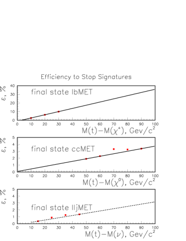
Figure 54: Efficiencies for the stop signatures studied in this report.

Figure 55: Sensitivity to searches for stop pair production in $\tilde{t}_{1}\rightarrow\tilde{\chi}^{+}_{1}b$ channel.

XXV.1.2 Reach in the $cc\not{\!\!E_{T}}$ topology

The decay $\tilde{t}_{1}\rightarrow c\tilde{\chi}^{0}_{1}$ gives rise to events presenting two acolinear charm jets and missing $E_{T}$. In our analysis, we assumed that this decay channel is dominant when it is kinematically allowed.

The main sources of SM backgrounds are the $W/Z$+jets production where the vector boson decays into a $e$ or $\mu$ that is not identified or into a $\tau$ which decays hadronically. There is also a small contribution from QCD multiple jet production and $t\bar{t}$ pairs. In order to extract the signal we required that

• the event must have 2 or 3 jets with $E_{T}>15$ GeV and $45^{\circ}<\Delta\phi(j_{1},j_{2})<165^{\circ}$;

• $\not{\!\!E_{T}}>40$ GeV and is not in the direction of the jets, i.e.,
  $45^{\circ}<\Delta\phi(\not{\!\!E_{T}},j)<165^{\circ}$;

• at least one jet is tagged as a charm jet, using secondary vertex information.

We exhibit in Fig. 56 the expect $5\sigma$ sensitivity of the RUN II for the search of $\tilde{t}_{1}\rightarrow c\tilde{\chi}^{0}_{1}$. As we can see, this channel will allow a search for stops with masses up to 160 GeV, depending on $m_{\tilde{\chi}^{0}_{1}}$, for an integrated luminosity of 2 fb^-1. The gap between the kinematical limit and the region of sensitivity is due to the low efficiency for this topology, as can be seen from Fig. 54, where the most stringent cut is on $E\hbox to0.0pt{\hss/}_{T}$. In order to close this gap we can lower the missing $E_{T}$ cut to 25 GeV in the search for $cc\not{\!\!E_{T}}$ topology provided secondary vertex information can be used at the trigger level.

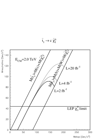
Figure 56: Sensitivity to searches for $\tilde{t}_{1}\rightarrow c\tilde{\chi}^{0}_{1}$ for several integrated luminosities.

XXV.1.3 Reach in the $j\ell^{+}\ell^{-}\not{\!\!E_{T}}$ topology

In the parameter space regions where the sleptons are light enough, it is possible for stops to decay into $b\ell\tilde{\nu}$ or $b\tilde{\ell}\nu$. In this scenario, the search for events presenting two leptons and a jet becomes important. Moreover, in this case it is not necessary to require a $b$-tagged jet. The main SM backgrounds for this topology are Drell-Yan and the production of $b\bar{b}$, $t\bar{t}$, and $W$+ jets. In order to select these events we required

• two leptons with $p_{T}(\ell_{1})>8$ GeV and $p_{T}(\ell_{2})>5$ GeV;

• at least one jet with $E_{T}>15$ GeV;

• $\not{\!\!E_{T}}>20$ GeV.

The reach of the stop search in the $j\ell^{+}\ell^{-}\not{\!\!E_{T}}$ channel is presented in Fig. 57 for several integrated luminosities. Clearly this channel will be able to probe stop masses up to 190 GeV for an integrated luminosity of 2 fb^-1.

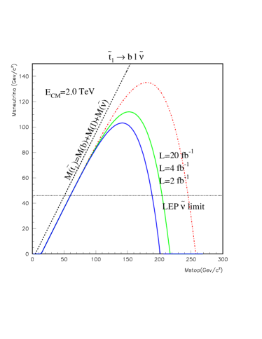
Figure 57: Sensitivity to searches for $\tilde{t}_{1}\rightarrow b\ell\tilde{\nu}$ or $b\nu\tilde{\ell}$ for different integrated luminosities.

XXV.2 Sbottom pair production

It is possible that $\tilde{b}_{1}$, the lighter of the two $b$-squark eigenstates, may be much lighter than other squarks. Moreover, in models (such as mSUGRA) with universal squark masses at some high scale, it is reasonable to suppose that $\tilde{b}_{1}\approx\tilde{b}_{L}$ as long as the bottom Yukawa coupling is small relative to its top counterpart.

The sbottom pair production signatures depend on the allowed sbottom decay channels. In this analysis, we assume that the gluino is so heavy that the decay $\tilde{b}_{1}\rightarrow b\tilde{g}$ is kinematically forbidden, and further, that the lightest neutralino ($\tilde{\chi}^{0}_{1}$) mass is such that the decay $\tilde{b}_{1}\rightarrow b\tilde{\chi}^{0}_{1}$ is always allowed. The other possible two-body decay modes are $\tilde{b}_{1}\rightarrow b\tilde{\chi}^{0}_{i}$ and $\tilde{b}_{1}\rightarrow t\tilde{\chi}^{+}_{i}$. Given the available center-of-mass energy at the Tevatron, it is sufficient to focus on the case where only the neutralino decays of $\tilde{b}_{1}$ are accessible.

We use ISAJET 7.37 ISAJET for our simulation, and we model the experimental conditions at the Tevatron through the toy calorimeter simulation package ISAPLT. We simulate calorimetry covering $-4<\eta<4$ with cell size $\Delta\eta\times\Delta\phi=0.1\times 5^{\circ}$. We take the hadronic (electromagnetic) energy resolution to be $50\%/\sqrt{E}$ ($15\%/\sqrt{E}$). Jets are defined as hadronic clusters with $E_{T}>15$ GeV within a cone with $\Delta R=\sqrt{\Delta\eta^{2}+\Delta\phi^{2}}=0.7$. We require that $|\eta_{j}|\leq 3.5$. Muons and electrons are classified as isolated if they have $p_{T}>10$ GeV, $|\eta(\ell)|<2$, and the visible activity within a cone of $R=0.3$ about the lepton direction is less than 5 GeV. For SVX tagged $b$-jets, we require a jet (using the above jet requirement) to have in addition $|\eta_{j}|<1$ and to contain a $B$-hadron with $p_{T}>15$ GeV. Then the jet is tagged as a $b$-jet with a 50% efficiency.

XXV.2.1 The ${\tilde{b}_{1}}\rightarrow\tilde{\chi}^{0}_{1}b$ case

Here we assume that $m_{\tilde{\chi}^{0}_{2}}>m_{\tilde{b}_{1}}-m_{b}$ so that $\tilde{b}_{1}\rightarrow b\tilde{\chi}^{0}_{1}$ with a branching fraction of essentially 100%. In this case, the signal naively consists of two $b$-jets recoiling against $E\hbox to0.0pt{\hss/}_{T}$ from the two neutralinos that escape detection. The dominant SM backgrounds come from $W+j$, $Z\rightarrow\nu\nu+j$, $Z\rightarrow\tau\tau+j$ and $t\bar{t}$ production. To enhance the signal relative to the SM background, we impose the following requirements, hereafter referred to as the basic cuts:

1. at least two jets with $p_{T}(j_{1})>30$ GeV, $p_{T}(j_{2})>20$ GeV;

2. at least one jet in $|\eta_{j}|<1$;

3. $E\hbox to0.0pt{\hss/}_{T}>50$ GeV;

4. $\Delta\phi(\vec{E\hbox to0.0pt{\hss/}_{T}},\vec{p}_{Tj})>30^{\circ}$;

5. for di-jet events only, $\Delta\phi(\vec{p}_{Tj1},\vec{p}_{Tj2})<150^{\circ}$;

6. at least one SVX tagged B;

7. no isolated leptons ($e$ or $\mu$).

The dominant SM background at 2 TeV is $t\bar{t}$ production; see Table 19. Because of the lepton veto, much of this background comes when one of the tops decays into a tau lepton that decays hadronically, while the other top decays completely hadronically. These events are, therefore, likely to have large jet multiplicity, in contrast to the signal. We are, therefore, led to impose the additional requirement,

1. $n_{j}=2,3\,,$

designed to further reduce the top background with relatively modest loss of signal. The corresponding background levels are shown in the second row of Table 19. The entry +8 in the first column denotes the cuts over and above the basic cuts 1-7. Indeed, we see that the top background is reduced by a factor 5, and no longer dominates. Now the background comes mainly from $Z\rightarrow\nu\nu+j$ events. Therefore we are led to impose, in addition to cuts 1-8, a further requirement,

1. $\Delta\phi({j_{1},j_{2}})\geq 90^{\circ}$,

which significantly reduces the vector boson backgrounds, as can be seen from the third row in Table 19. For higher integrated luminosity, like 25 $fb^{-1}$, the high event rate makes it possible to require double $b$-tagging,

1. $n_{b}\geq 2$,

to greatly reduce the vector boson background. Finally, we also considered the cut,

1. $m_{j_{1},j_{2}}\leq 60$ GeV, where $j_{1}$ and $j_{2}$ are the two highest $p_{T}$ untagged jets in the event. If an event has less than two untagged jets, we retain it as part of the signal.

Table 19: Standard Model background cross sections in fb to the $b$-squark signal after the basic cuts 1-7 described in the text, as well as after additional cuts designed to further reduce backgrounds. The “plus entries” in the first column refer to the cuts in addition to the basic cuts; for instance, the last row has cuts 1-8 together with cut 11. We take $m_{t}=175$ GeV.

CUT	$W+j$	$Z\rightarrow\nu\nu+j$	$Z\rightarrow\tau\tau+j$	$t\bar{t}$	$Total$
Basic	65.5	92.4	2.6	195	356
$+8$	51.6	80.6	2.1	36.7	172
$+8+9$	21.9	26.2	0.9	28.0	77
$+10$	5.6	7.2	0.1	37.5	50.4
$+8+10$	3.8	6.6	0.1	6.7	17.2
$+10+11$	5.0	6.6	0	11.7	23.3

Turning to the signal, the sbottom production cross section is completely determined by $m_{\tilde{b}_{1}}$ and $m_{\tilde{\chi}^{0}_{1}}$. The $5\sigma$ reach of a 2 TeV $p\bar{p}$ collider bpt is shown in Fig. 59. In addition, we also require the signal to exceed 20% of the background. The diagonal solid line marks the boundary of the region where $m_{\tilde{b}_{1}}\geq m_{\tilde{\chi}^{0}_{1}}+m_{b}$. With our assumptions, we must be below this line, since otherwise, $\tilde{b}_{1}$ would be the LSP. The dot-dashed contour shows the reach that should be attainable (using cuts 1-8) with an integrated luminosity of 2 fb^-1. The dotted lines denote signal cross sections after these cuts. Preliminary CDF studies indicate that the attainable limits do not change significantly when a full detector simulation is carried out regi ; see Fig. 59.

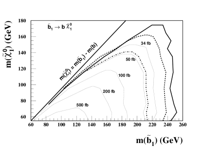
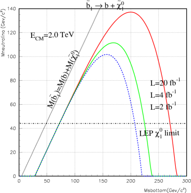
Figure 58: The region of the $m_{\tilde{b}_{1}}-m_{\tilde{\chi}^{0}_{1}}$ plane that can be probed at a 2 TeV $p\bar{p}$ collider, assuming that $\tilde{b}_{1}\rightarrow b\tilde{\chi}^{0}_{1}$ and that $\tilde{\chi}^{0}_{1}$ escapes detection. The sbottom signal should be detectable with the observability criteria defined in the text in the region below the dot-dashed, dashed and solid contours for an integrated luminosity of 2 fb^-1, 10 fb^-1 and 25 fb^-1. Also shown in the figure are contours of constant signal cross section after cuts 1-8 for the 2 fb^-1 case. The 34 fb contour marks the $0.2B$ level that we require as a minimum for the signal. The diagonal line marks the boundary of the region beyond which $m_{\tilde{b}_{1}}>m_{b}+m_{\tilde{\chi}^{0}_{1}}$.

Figure 59: CDF discovery potential of bottom squarks in the channel $\tilde{b}_{1}\rightarrow b\tilde{\chi}^{0}_{1}$.

XXV.2.2 The $m_{\tilde{b}_{1}}>m_{b}+m_{\tilde{\chi}^{0}_{2}}$ case

The signal now depends on the branching fraction for the decay $\tilde{b}_{1}\rightarrow b\tilde{\chi}^{0}_{2}$, as well as the decay pattern of $\tilde{\chi}^{0}_{2}$. In other words, the signal depends not only on the $b$-squark mixing angle but also on the parameters of the neutralino mass matrix. To make our analysis tractable, we will assume that $\tilde{b}_{1}\approx\tilde{b}_{L}$. We will further assume that $|\mu|$ is much larger than electroweak gaugino masses. Assuming gaugino mass unification, the two lighter neutralinos are approximately the hypercharge gaugino and the $SU(2)$-gaugino, with $m_{\tilde{\chi}^{0}_{2}}\approx m_{\tilde{\chi}^{+}_{1}}\approx 2m_{\tilde{\chi}^{0}_{1}}$. Note that these assumptions fix the branching fraction for $\tilde{b}_{1}\rightarrow b\tilde{\chi}^{0}_{1,2}$ decays in terms of the sparticle masses. It is also worth pointing out that if $\tilde{\chi}^{0}_{2}\simeq SU(2)$-gaugino, it essentially decouples from $\tilde{b}_{R}$, so that the maximum impact of the $\tilde{b}_{1}\rightarrow b\tilde{\chi}^{0}_{2}$ indeed occurs when $\tilde{b}_{1}=\tilde{b}_{L}$.

Since we are interested in seeing how much the reach of the Tevatron may be reduced from that shown in Fig. 59, we consider extreme limits for how $\tilde{\chi}^{0}_{2}$ might decay FN2 . If $\tilde{\chi}^{0}_{2}$ dominantly decays to leptons via $\tilde{\chi}^{0}_{2}\rightarrow\ell\bar{\ell}\tilde{\chi}^{0}_{1}$, sbottom pair production would result in characteristic $bb+4\ell+E\hbox to0.0pt{\hss/}_{T}$ and $bb+2\ell+jets+E\hbox to0.0pt{\hss/}_{T}$ events for which the background is small, and the corresponding reach, presumably, larger than that in Fig. 59. If $\tilde{\chi}^{0}_{2}\rightarrow b\bar{b}\tilde{\chi}^{0}_{1}$ it may be possible to reduce the background (and hence increase the reach) by requiring two (or more) $b$-tags. The worst case “realistic” scenario is when $\tilde{\chi}^{0}_{2}$ decays into jets which are not amenable to any tagging FN3 . To simulate this situation, we have forced $\tilde{\chi}^{0}_{2}$ to decay via $\tilde{\chi}^{0}_{2}\rightarrow u\bar{u}\tilde{\chi}^{0}_{1}$ and run these events through our simulation, and once again obtained the reach for the three choices of integrated luminosity in Fig. 59.

The results of our analysis for this case are illustrated in Fig. 60. The upper diagonal line is as in Fig. 59, while the lower line is where $m_{\tilde{b}_{1}}=2m_{\tilde{\chi}^{0}_{1}}+m_{b}\simeq m_{\tilde{\chi}^{0}_{2}}+m_{b}$. In our analysis, we have adjusted $A_{b}$ to cancel the off diagonal term in the sbottom mass matrix in order to make $\tilde{b}_{1}=\tilde{b}_{L}$. We have fixed $\mu=500$ GeV and $\tan\beta=2$; this value of $\mu$ is large enough for $\tilde{\chi}^{0}_{1}$ and $\tilde{\chi}^{0}_{2}$ to be gauginos to a very good approximation. When the decay $\tilde{b}_{1}\rightarrow b\tilde{\chi}^{0}_{2}$ is inaccessible, the reach should be as given by our analysis above; i.e., the reach illustrated by the dot-dashed, dashed and solid contours until just above this line, is identical to that in Fig. 59. The contours below this line show the extent to which the reach might be reduced if the $\tilde{b}_{1}$ can also decay to $\tilde{\chi}^{0}_{2}$. These contours in Fig. 60 turn inwards just slightly above this line precisely because the relation $m_{\tilde{\chi}^{0}_{2}}=2m_{\tilde{\chi}^{0}_{1}}$ is slightly violated by our finite choice of $\mu$.

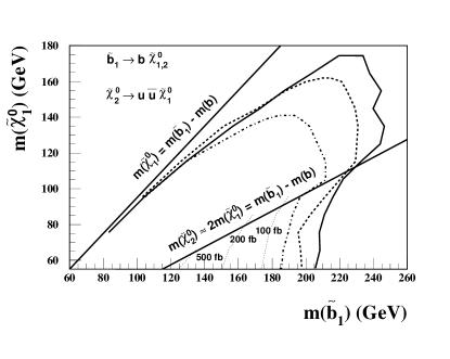
Figure 60: The same as Fig. 59 except that the decay $\tilde{b}_{1}\rightarrow b\tilde{\chi}^{0}_{2}$ is also allowed when kinematically accessible below the lower diagonal line. To illustrate the largest degradation of the reach in this scenario, we assume that $\tilde{\chi}^{0}_{2}$ always decays via $\tilde{\chi}^{0}_{2}\rightarrow u\bar{u}\tilde{\chi}^{0}_{1}$. The dotted lines are again contours of fixed cross section after the basic cuts 1-7. The dot-dashed contour that denotes our projection of the MI reach also corresponds to $S=0.2B$.

In summary, assuming that $\tilde{b}_{1}\rightarrow b\tilde{\chi}^{0}_{1}$ and that $\tilde{\chi}^{0}_{1}$ escapes detection, we have shown that it should be possible for experiments at the MI to detect $b$-squark signals over SM backgrounds for $m_{\tilde{b}_{1}}\leq 210$ GeV, even if the LSP is quite heavy. The capability of tagging $b$-jets in the central region with high efficiency and purity is crucial for this detection. The reach may be somewhat degraded if sbottom can also decay into $\tilde{\chi}^{0}_{2}$. We have argued that in many models (with $\tilde{\chi}^{0}_{1}$ as a stable LSP) this degradation is typically smaller than 30–40 GeV.

XXV.3 Gluino production

The gluino pair production takes place through gluon-gluon and quark-quark fusions, and consequently, the production cross section depends only on the gluino mass. However, the signals for gluino production depend on properties of all sparticles lighter than these since they can appear in the gluino cascade decays. Moreover, its signal comes mixed with the ones due to the production of squark as well as gluino squark pairs.

XXV.3.1 $E\hbox to0.0pt{\hss/}_{T}+$ jets channel

The canonical signature of supersymmetry is multi-jet events with a large $E\hbox to0.0pt{\hss/}_{T}$ etj ; see Fig. 61. This signal can originate from many SUSY particle production like $\tilde{g}\tilde{g}$ or $\tilde{q}\tilde{q}$. The main SM backgrounds for this channel are single and pair production of $W$’s and/or $Z$’s in association with jets, $t\bar{t}$, and QCD events with $E\hbox to0.0pt{\hss/}_{T}$ due to mismeasurement of the jets. In order to enhance the signal and suppress the backgrounds we imposed the following cuts ncpt :

• jet multiplicity $n_{\rm jet}\geq 2$;

• transverse sphericity $S_{T}>0.2$;

• $E\hbox to0.0pt{\hss/}_{T}>40$ GeV;

• the missing energy does not point along a jet, i.e. $\Delta\phi(\vec{E\hbox to0.0pt{\hss/}_{T}},\vec{E}^{j}_{T})>30^{\circ}$;

• $E_{T}(j_{1})~{},~{}E_{T}(j_{2})>E_{T}^{c}$ and $E\hbox to0.0pt{\hss/}_{T}>E_{T}^{c}$ where the parameter $E_{T}^{c}$ was adjusted as described below;

• no isolated leptons.

Figure 61: $E\hbox to0.0pt{\hss/}_{T}$ distribution for $\tan\beta=2$, $\mu<0$, $A_{0}=0$, $m_{0}=100$ GeV, and $m_{1/2}=70$ GeV, which corresponds to $m_{\tilde{q}}=207$ GeV and $m_{\tilde{g}}=215$ GeV.

We considered a signal to be observable if, for a given integrated luminosity, we have (i) at least 5 signal events, (ii) the statistical significance of the signal exceeds $5\sigma$, and (iii) the signal is larger than 20% of the background. We checked the observability of the signal for $E_{T}^{c}=15$, 40, 60, 80, 100, 120, and 140 GeV and considered the signal to be observable if it is so for any one of the values of $E_{T}^{c}$. In our analysis we used ISAJET to generate the signal and backgrounds and assumed a toy calorimeter similar to the one described in the sbottom analyses.

In Fig. 62, we present the observable regions of the plane $m_{0}\times m_{1/2}$ according to the above criteria ncpt . This figure was obtained for $\tan\beta=2$ (10) and both signs of $\mu$ with $A_{0}$ being fixed to zero. As we can see from this figure, with a data sample of 2 fb^-1, the Tevatron experiments should be able to probe $m_{1/2}$ up to 150 GeV, corresponding to $m_{\tilde{g}}\simeq 400$ GeV, if $m_{0}<200$ GeV.

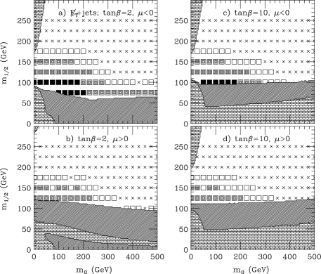
Figure 62: Regions of the $m_{0}\times m_{1/2}$ plane where the multi-jets plus $E\hbox to0.0pt{\hss/}_{T}$ signal is observed at a 2 TeV $p\bar{p}$ collider. We considered three values for the integrated luminosity: 100 pb^-1 (black squares), 2 fb^-1 (gray squares), and 25 fb^-1 (white squares). The bricked regions are excluded by theoretical constraints and the shaded regions are excluded by experiment.

XXV.3.2 Multijet plus leptons and $E\hbox to0.0pt{\hss/}_{T}$ channels

The cascade decay of gluinos (or squarks) can also give rise to leptons in addition to jets and missing $E_{T}$. We further classify the events by their isolated lepton ($e$ or $\mu$) content as follows:

• $1\ell$ events with exactly one isolated lepton satisfying $E_{T}(\ell)>10$ GeV. To reduce the background from $W$ production, we also required $M_{T}(\ell,E\hbox to0.0pt{\hss/}_{T})>100$ GeV;

• Opposite sign ($OS$) dilepton events with exactly two unlike sign isolated leptons, where we required $E_{T}(\ell_{1})>10$ GeV;

• Same sign ($SS$) dilepton events with exactly two same sign isolated leptons, again with $E_{T}(\ell_{1})>10$ GeV;

• $3\ell$ events, with exactly three isolated leptons with $E_{T}(\ell_{1})>10$ GeV. We veto events with $|M(\ell^{+}\ell^{-})-M_{Z}|<8$ GeV.

A detailed analysis of the above signatures ncpt indicates that the maximal reach is still obtained in the $E\hbox to0.0pt{\hss/}_{T}$ plus multiplet channel, except for isolated values of SUGRA parameters where the trilepton channel has a larger reach (see Fig. 63).

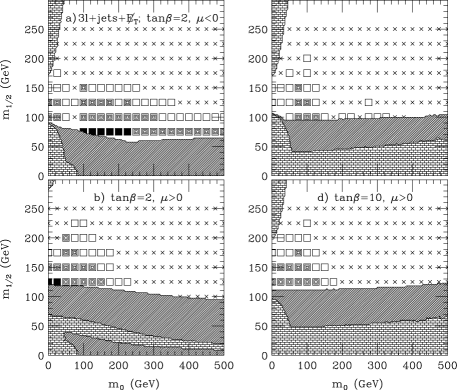
Figure 63: The same as Fig. 62 except for the multijet plus $3\ell$ and $E\hbox to0.0pt{\hss/}_{T}$ channel.

XXV.3.3 Large $\tan\beta$

At large $\tan\beta$ the tau and bottom Yukawa couplings become comparable to the electroweak gauge couplings and even to the top Yukawa coupling. This has a significant impact tb on the search for supersymmetry at colliders. For large $\tan\beta$ the lightest tau slepton and bottom squark can be considerably lighter than the corresponding sleptons and squarks of the first two generations. Moreover, gluino, chargino and neutralino decays to third generation particles are significantly enhanced when $\tan\beta$ is large.

The phenomenological implications related to large values of $\tan\beta$ are: the Tevatron signals in multilepton ($e$ and $\mu$) channels are greatly reduced while there could be new signals involving $b$-jets and $\tau$-leptons via which to search for SUSY tb . Furthermore, for very large $\tan\beta$ the greatest reach is attained in the multi-jet$+E\hbox to0.0pt{\hss/}_{T}$ signature. Figure 51 (earlier in this report) shows the reach of the Tevatron upgrades for large and small $\tan\beta$, where a point is considered to be accessible if there is a channel leading to a $5\sigma$ effect. In this analyses the same cuts of the previous subsection were used tb . We can see from this figure that the SUSY sensitivity of the Tevatron upgrades is reduced as $\tan\beta$ increases.

XXVI Trilepton Signal of Minimal Supergravity at the Upgraded Tevatron

XXVI.1 Introduction

In this report, we assess the prospects of discovering the trilepton signal along with missing transverse energy ($3\ell+\ \hbox{{$E$}\kern-6.00006pt\hbox{/}}_{T}$) Wdecay ; Trilepton1 ; Trilepton2 ; Trilepton3 ; BCDPT ; Madison1 ; Madison2 ; Matchev1 ; Matchev2 ; Baer&Tata ; D0-3l ; CDF-3l in the minimal supergravity model (mSUGRA) at the upgraded Tevatron with 2 TeV center of mass energy. We assume each of the CDF and the DØ experiments will accumulate an integrated luminosity (${\cal L}$) of 2 fb^-1 at Run II. In addition, we consider a possible upgrade of the Tevatron luminosity to $10^{33}$ cm^-2 s^-1 at Run III and take the corresponding integrated luminosity to be ${\cal L}=30$ fb^-1 Run3 . The major source of this signal is associated production of the lightest chargino ($\tilde{\chi}^{\pm}_{1}$) and the second lightest neutralino ($\tilde{\chi}^{0}_{2}$) with decays to leptons.

In the mSUGRA unified model, the sleptons ($\tilde{\ell}$), the lighter chargino ($\tilde{\chi}^{\pm}_{1}$) and the lighter neutralinos ($\tilde{\chi}^{0}_{1},\tilde{\chi}^{0}_{2}$) are typically less massive than gluinos and squarks. Because of this, the $3\ell+\ \hbox{{$E$}\kern-6.00006pt\hbox{/}}_{T}$ signal from associated production and decays of $\tilde{\chi}^{\pm}_{1}\tilde{\chi}^{0}_{2}$ is one of the most promising channels for supersymmetric (SUSY) particle searches at the Tevatron. The background to this signal from processes in the Standard Model (SM) can be greatly reduced with suitable cuts. In most of the mSUGRA parameter space, the weak-scale gaugino masses are related to the universal gaugino mass parameter $m_{1/2}$ by $m_{\tilde{\chi}^{0}_{1}}\sim 0.4m_{1/2}$ and $m_{\tilde{\chi}^{\pm}_{1}}\sim m_{\tilde{\chi}^{0}_{2}}\sim 0.8m_{1/2}$. Consequently, this discovery channel could provide valuable information about the value of $m_{1/2}$. We consider universal boundary conditions at $M_{\rm GUT}$ with a common gaugino mass $m_{1/2}$ and a common scalar mass $m_{0}$ to study the production cross section and decay branching fractions of $\tilde{\chi}^{\pm}_{1}$ and $\tilde{\chi}^{0}_{2}$. Non-universal boundary conditions among sfermion masses sfermions-3l or the gaugino masses gauginos-3l could change the production cross section and branching fractions of the charginos and neutralinos. For $m_{1/2}=$ 200 GeV and $\tan\beta\mathrel{\raisebox{-2.58334pt}{$\stackrel{{\scriptstyle\textstyle<}}{{\sim}}$}}25$, a non-universality among sfermions may significantly enhance the trilepton signal when 50 GeV $\mathrel{\raisebox{-2.58334pt}{$\stackrel{{\scriptstyle\textstyle<}}{{\sim}}$}}m_{0}\mathrel{\raisebox{-2.58334pt}{$\stackrel{{\scriptstyle\textstyle<}}{{\sim}}$}}$ 130 GeV sfermions-3l .

The Yukawa couplings of the bottom quark ($b$) and the tau lepton ($\tau$) are proportional to $\sec\beta$ and are thus greatly enhanced when $\tan\beta$ is large. In SUSY grand unified theories, the masses of the third generation sfermions are consequently very sensitive to the value of $\tan\beta$. As $\tan\beta$ increases, the lighter tau slepton ($\tilde{\tau}_{1}$) and the lighter bottom squark ($\tilde{b}_{1}$) become lighter than charginos and neutralinos while other sleptons and squarks are heavy. Then, $\tilde{\chi}^{\pm}_{1}$ and $\tilde{\chi}^{0}_{2}$ can dominantly decay into final states with tau leptons via real $\tilde{\tau}_{1}$.

The relevance of $\tau$ leptons in the production and decays of $\tilde{\chi}^{\pm}_{1}\tilde{\chi}^{0}_{2}$, are illustrated in Figure 64, where the product of the cross section $\sigma(p\bar{p}\rightarrow\tilde{\chi}^{\pm}_{1}\tilde{\chi}^{0}_{2}+X)$ and the branching fraction $B(\tilde{\chi}^{\pm}_{1}\tilde{\chi}^{0}_{2}\rightarrow 3\;{\rm leptons}\;+\ \hbox{{$E$}\kern-6.00006pt\hbox{/}}_{T})$ versus $\tan\beta$ is presented with $\mu>0$, $m_{1/2}=200$ GeV, $m_{0}=$ 100 and 200 GeV, for four final states (a) $\tau\tau\tau$, (b) $\tau\tau\ell$, (c) $\tau\ell\ell$ and (d) $\ell\ell\ell$, where $\ell=e$ or $\mu$. For $m_{0}\mathrel{\raisebox{-2.58334pt}{$\stackrel{{\scriptstyle\textstyle<}}{{\sim}}$}}$ 200 GeV and/or $\tan\beta\mathrel{\raisebox{-2.58334pt}{$\stackrel{{\scriptstyle\textstyle>}}{{\sim}}$}}40$, channels with at least one $\tau$ lepton are dominant.

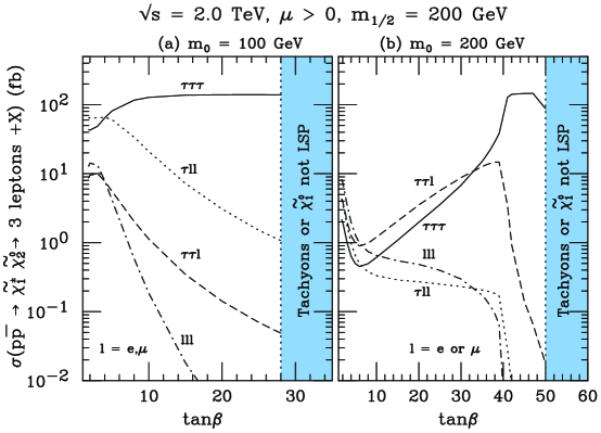
Figure 64: Cross section of $p\bar{p}\rightarrow\tilde{\chi}^{\pm}_{1}\tilde{\chi}^{0}_{2}\rightarrow 3\;{\rm leptons}\;+X$ without cuts at $\sqrt{s}=2$ TeV versus $\tan\beta$, with $\mu>0$, $m_{1/2}=200$ GeV, $m_{0}=$ 100 GeV for (a) $\tau\tau\tau$ (solid), (b) $\tau\tau\ell$ (dot-dash), (c) $\tau\ell\ell$ (dash) and (d) $\ell\ell\ell$ (dot), where $\ell=e$ or $\mu$.

One way to detect $\tau$ leptons is through their one prong and three prong hadronic decays. The CDF and the DØ collaborations are currently investigating the efficiencies for detecting these modes and for possibly implementing a $\tau$ trigger. Recently, it has been suggested that the $\tau$ leptons in the final state may be a promising way to search for $\tilde{\chi}^{\pm}_{1}\tilde{\chi}^{0}_{2}$ production at the Tevatron if excellent $\tau$ identification becomes feasible BCDPT ; Matchev1 ; Wells .

Another way of exploiting the $\tau$ signals, that we consider in this report, is to detect the soft electrons and muons from leptonic $\tau$ decays by employing softer but realistic $p_{T}$ cuts on the leptons Madison1 ; Madison2 . We find that this can considerably improve the trilepton signal significance from $\tilde{\chi}^{\pm}_{1}\tilde{\chi}^{0}_{2}$ production.

XXVI.2 Cross Section and Branching Fractions

In hadron collisions, associated production of chargino and neutralino occurs via quark-antiquark annihilation in the $s$-channel through a $W$ boson ($q\bar{q^{\prime}}\rightarrow W^{\pm}\rightarrow\tilde{\chi}^{\pm}_{1}\tilde{\chi}^{0}_{2}$) and in the $t$ and $u$-channels through squark ($\tilde{q}$) exchanges. If the squarks are light, a destructive interference between the $W$ boson and the squark exchange amplitudes can suppress the cross section by as much as $40\%$ compared to the $s$-channel contribution alone. For squarks much heavier than the gauge bosons, the effect of negative interference is reduced and the $s$-channel $W$-resonance amplitude dominates.

In Figure 65, we present branching fractions of $\tilde{\chi}^{0}_{2}$ versus $\tan\beta$ with $\mu>0$ as well as $\mu<0$ for $m_{1/2}=200$ GeV and several values of $m_{0}$. For $\tan\beta\mathrel{\raisebox{-2.58334pt}{$\stackrel{{\scriptstyle\textstyle<}}{{\sim}}$}}5$, the branching fractions are sensitive to the sign of $\mu$.

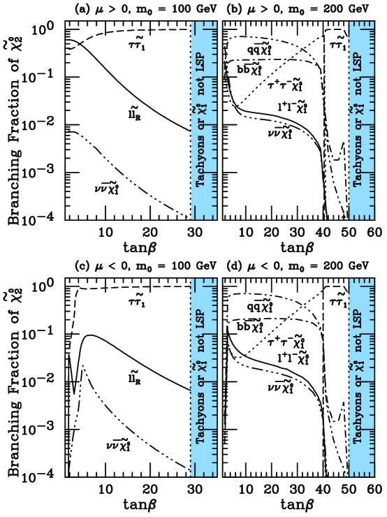
Figure 65: Branching fractions of $\tilde{\chi}^{0}_{2}$ decays into various channels versus $\tan\beta$ with $m_{1/2}=$ 200 GeV, for $m_{0}=100$ GeV and 200 GeV.

For $\mu>0$ and $\tan\beta\sim 3$, we have found that:

• For $m_{0}\mathrel{\raisebox{-2.58334pt}{$\stackrel{{\scriptstyle\textstyle<}}{{\sim}}$}}100$ GeV, $\tilde{\chi}^{0}_{2}$ decays dominantly to $\tilde{\ell}_{R}\ell$ and $\tilde{\tau}_{1}\tau$, and $\tilde{\chi}^{\pm}_{1}$ decays into $\tilde{\tau}_{1}\nu$,

• For 120 GeV $\mathrel{\raisebox{-2.58334pt}{$\stackrel{{\scriptstyle\textstyle<}}{{\sim}}$}}m_{0}\mathrel{\raisebox{-2.58334pt}{$\stackrel{{\scriptstyle\textstyle<}}{{\sim}}$}}$ 170 GeV, the $\tilde{\chi}^{\pm}_{1}\tilde{\chi}^{0}_{2}\rightarrow 3\ell+\ \hbox{{$E$}\kern-6.00006pt\hbox{/}}_{T}$ branching fraction is still significant due to light virtual sleptons.

• For $m_{0}\mathrel{\raisebox{-2.58334pt}{$\stackrel{{\scriptstyle\textstyle>}}{{\sim}}$}}$ 180 GeV, $\tilde{\chi}^{\pm}_{1}$ and $\tilde{\chi}^{0}_{2}$ dominantly decay into $q\bar{q}^{\prime}\tilde{\chi}^{0}_{1}$.

For $\mu<0$ and $\tan\beta\sim 3$, we have found that:

• For $m_{0}\mathrel{\raisebox{-2.58334pt}{$\stackrel{{\scriptstyle\textstyle<}}{{\sim}}$}}$ 140 GeV, $\tilde{\chi}^{0}_{2}$ dominantly decays to $\tilde{\nu}_{L}\nu$, $\tilde{\ell}_{R}\ell$, and $\tilde{\tau}_{1}\tau$, and $\tilde{\chi}^{\pm}_{1}$ decays into $\tilde{\nu}_{L}\ell$ and $\tilde{\tau}_{1}\nu$.

• For 140 GeV $\mathrel{\raisebox{-2.58334pt}{$\stackrel{{\scriptstyle\textstyle<}}{{\sim}}$}}m_{0}\mathrel{\raisebox{-2.58334pt}{$\stackrel{{\scriptstyle\textstyle<}}{{\sim}}$}}$ 160 GeV, the $\tilde{\chi}^{\pm}_{1}\tilde{\chi}^{0}_{2}\rightarrow 3\ell+\ \hbox{{$E$}\kern-6.00006pt\hbox{/}}_{T}$ branching fraction is still significant due to light virtual sleptons.

• For $m_{0}\mathrel{\raisebox{-2.58334pt}{$\stackrel{{\scriptstyle\textstyle>}}{{\sim}}$}}$ 170 GeV, $\tilde{\chi}^{\pm}_{1}$ and $\tilde{\chi}^{0}_{2}$ dominantly decay into $q\bar{q}^{\prime}\tilde{\chi}^{0}_{1}$.

For $\mu>0$ and $m_{0}\sim$ 200 GeV, $\tilde{\chi}^{0}_{2}$ dominantly decays (i) into $\tau\bar{\tau}\tilde{\chi}^{0}_{1}$ for $25\mathrel{\raisebox{-2.58334pt}{$\stackrel{{\scriptstyle\textstyle<}}{{\sim}}$}}\tan\beta\mathrel{\raisebox{-2.58334pt}{$\stackrel{{\scriptstyle\textstyle<}}{{\sim}}$}}40$, (ii) into $\tau\tilde{\tau}_{1}$ for $\tan\beta\mathrel{\raisebox{-2.58334pt}{$\stackrel{{\scriptstyle\textstyle>}}{{\sim}}$}}40$. For $m_{0}\mathrel{\raisebox{-2.58334pt}{$\stackrel{{\scriptstyle\textstyle<}}{{\sim}}$}}300$ GeV and $\tan\beta\mathrel{\raisebox{-2.58334pt}{$\stackrel{{\scriptstyle\textstyle>}}{{\sim}}$}}35$, both $\tilde{\tau}_{1}$ and $\tilde{b}_{1}$ can be lighter than other sfermions, and $\tilde{\chi}^{\pm}_{1}$ and $\tilde{\chi}^{0}_{2}$ can decay dominantly into final states with $\tau$ or $b$ via virtual or real $\tilde{\tau}_{1}$ and $\tilde{b}_{1}$.

XXVI.3 Discovery Potential at the Tevatron

The ISAJET 7.44 event generator program ISAJET-3l with the parton distribution functions of CTEQ3L CTEQ-3l is employed to calculate the $3\ell+\ \hbox{{$E$}\kern-6.00006pt\hbox{/}}_{T}$ signal from all possible sources of SUSY particles. An energy resolution of $\frac{0.7}{\sqrt{E}}$ for the hadronic calorimeter and $\frac{0.15}{\sqrt{E}}$ for the electromagnetic calorimeter is assumed. Jets are defined to be hadron clusters with $E_{T}>15$ GeV in a cone with $\Delta R\equiv\sqrt{\Delta\eta^{2}+\Delta\phi^{2}}=0.7$. Leptons with $p_{T}>5$ GeV and within $|\eta_{\ell}|<2.5$ are considered to be isolated if the hadronic scalar $E_{T}$ in a cone with $\Delta R=0.4$ about the lepton is smaller than 2 GeV.

After suitable cuts, there are two major sources of the SM background Trilepton2 ; Trilepton3 ; Madison1 ; Madison2 ; Matchev1 ; Matchev2 ; Baer&Tata ; Chanowitz ; Ellis : (i) $q\bar{q}\rightarrow W^{*}Z^{*},W^{*}\gamma^{*}\rightarrow\ell\nu\ell\bar{\ell}$ or $\ell^{\prime}\nu^{\prime}\ell\bar{\ell}$ ($\ell=e$ or $\mu$) with one or both gauge bosons being virtual, and (ii) $q\bar{q}\rightarrow W^{*}Z^{*},W^{*}\gamma^{*}\rightarrow\ell\nu\tau\bar{\tau}$ or $\tau\nu\ell\bar{\ell}$ and subsequent $\tau$ leptonic decays. We have employed the programs MADGRAPH Madgraph and HELAS Helas to calculate the cross section of $p\bar{p}\rightarrow 3l+\ \hbox{{$E$}\kern-6.00006pt\hbox{/}}_{T}+X$ via four subprocesses (i) $q\bar{q}^{\prime}\rightarrow e^{+}\nu_{e}\mu^{+}\mu^{-}$, (ii) $q\bar{q}^{\prime}\rightarrow e^{+}\nu_{e}e^{+}e^{-}$, (iii) $q\bar{q}^{\prime}\rightarrow e^{+}\nu_{e}\tau^{+}\tau^{-}$, and (iv) $q\bar{q}^{\prime}\rightarrow\tau^{+}\nu_{\tau}e^{+}e^{-}$, including contributions from intermediate states with $W^{*}Z^{*}$, $W^{*}\gamma^{*}$, and other diagrams. We have also evaluated contributions from $q\bar{q}\rightarrow\tau^{+}\tau^{-}e^{+}e^{-}$ via $Z^{*}Z^{*}$, $Z^{*}\gamma^{*}$, and $\gamma^{*}\gamma^{*}$, with one leptonic and one hadronic tau decays. We use ISAJET to calculate the background from $t\bar{t}$.

We found that most $\ell_{3}$’s from the $\tilde{\chi}^{\pm}_{1}\tilde{\chi}^{0}_{2}$ decays have relatively smaller $p_{T}$ than the $\ell_{3}$’s from the backgrounds. Therefore, it is very important to have a soft acceptance cut on $p_{T}(\ell_{3})$ to retain the trilepton events from $\tilde{\chi}^{\pm}_{1}\tilde{\chi}^{0}_{2}$ decays. Our acceptance cuts are chosen to be consistent with the experimental cuts proposed for Run II Teruki ; Jane-3l at the Tevatron as follows:

$$p_{T}(\ell_{1}) > 11\;{\rm GeV},\;\;p_{T}(\ell_{2})>7\;{\rm GeV},\;\;p_{T}(\ell_{3})>5\;{\rm GeV},$$

$$|\eta(\ell_{1},\ell_{2},\ell_{3})| < 2.0,$$

$${\rm at\;\;least\;\;one}\;\;\ell\;\;{\rm with}\;\;p_{T}(\ell) > 11\;{\rm GeV}\;\;{\rm and}\;\;|\eta(\ell)|<1.0,$$

$$\ \hbox{{$E$}\kern-6.00006pt\hbox{/}}_{T} > 25\;\;{\rm GeV},$$

$$|M_{\ell\ell}-M_{Z}| \geq 10\;\;{\rm GeV}$$

$$M_{\ell\ell} \geq 12\;\;{\rm GeV}$$ (193)

To further reduce the background from $W^{*}Z^{*}$ and $W^{*}\gamma^{*}$, we require that Madison2 ; Baer&Tata

$$|M_{\ell\ell}-M_{Z}| \geq 15\;\;{\rm GeV}\;\;(Z-{\rm veto}),$$

$$M_{\ell\ell} \geq 18\;\;{\rm GeV}\;\;(\gamma-{\rm veto}),$$

$$M_{T}(\ell^{\prime},\ \hbox{{$E$}\kern-6.00006pt\hbox{/}}_{T}) \leq 65\;\;{\rm GeV}\;\;{\rm or}\;\;M_{T}(\ell^{\prime},\ \hbox{{$E$}\kern-6.00006pt\hbox{/}}_{T})\geq 85\;\;{\rm GeV}\;\;(W-{\rm veto}),$$ (194)

where $M_{\ell\ell}$ is the invariant mass for any pair of leptons with the same flavor and opposite signs, and $M_{T}(\ell^{\prime},\ \hbox{{$E$}\kern-6.00006pt\hbox{/}}_{T})$ is the transverse mass of the remaining lepton.

We have also checked backgrounds from the production of $Z+jets$ and $W+jets$. Some $3\ell$ events could be generated from $W+jets$, leading to sizable backgrounds; these sources always had $b\rightarrow c\ell\nu$ followed by $c\rightarrow s\ell\nu$, so that these sources of background could be removed by imposing an angular separation cut between the isolated leptons, giving a background consistent with zero. This angular separation cut causes no signal loss.

The effect of cuts on the signal and background is demonstrated in Table 20. The trileptons come from $\tilde{\chi}^{\pm}_{1}\tilde{\chi}^{0}_{2}$ production as well as additional SUSY particle sources that are discussed in the next section. The cross sections of the signal with $m_{1/2}=200$ GeV, $m_{0}=100$ GeV, and several values of $\tan\beta$, along with backgrounds from (i) $\ell^{\prime}\nu^{\prime}\ell\bar{\ell}$, (ii) $\ell\nu\ell\bar{\ell}$, (iii) $\ell\nu\tau\bar{\tau}$, (iv) $\tau\nu_{\tau}\ell\bar{\ell}$, (v) $\ell\bar{\ell}\tau\bar{\tau}$, and (vi) $t\bar{t}$. We present cross sections with six sets of cuts: (a) Basic Cuts Madison1 ; Madison2 : cuts in Eq. (193); (b) Soft Cuts A1 Madison2 : cuts in Eqs. (193) and (194); (c) Soft Cuts A2 Madison2 : the same cuts as soft cuts A1, except requiring 18 GeV $\leq M_{\ell\ell}\leq$ 75 GeV; (d) Soft Cuts B Baer&Tata : cuts in Eq. (193), $20\;\;{\rm GeV}\leq M_{\ell\ell}\leq 80\;\;{\rm GeV}$, and $M_{T}(\ell^{\prime},\ \hbox{{$E$}\kern-6.00006pt\hbox{/}}_{T})\leq 60\;\;{\rm GeV}$ or $M_{T}(\ell^{\prime},\ \hbox{{$E$}\kern-6.00006pt\hbox{/}}_{T})\geq 85\;\;{\rm GeV}$; (e) Hard Cuts A Madison2 : the same cuts as soft cuts A1, except requiring $M_{\ell\ell}\geq 12\;\;{\rm GeV}$, and $p_{T}(\ell_{1},\ell_{2},\ell_{3})>$ 20, 15, and 10 GeV; (f) Hard Cuts B Baer&Tata : the same cuts as in soft cuts B, except requiring 12 GeV $\leq M_{\ell\ell}\leq$ 80 GeV, and $p_{T}(\ell_{1},\ell_{2},\ell_{3})>$ 20, 15, and 10 GeV. The reach with any set of soft cuts is qualitatively quite similar. Hardening the cuts generally results in a reduced reach over much of parameter space, but may possibly lead to an incremental increase in the reach for the large values of $m_{1/2}$ and $m_{0}$. A more strict cut to require $M_{\ell\ell}<75$ GeV as in soft cuts A2 can further reduce the backgrounds from $\ell^{\prime}\nu^{\prime}\ell\bar{\ell}$ as well as $\ell\nu\ell\bar{\ell}$ with a slight reduction in the trilepton signal for most SUGRA parameters and might slightly improve the statistical significance. For brevity, we will present reach results with soft cuts A1 in this report.

Table 20: The cross section of $p\bar{p}\rightarrow{\rm SUSY\;\;particles}\rightarrow 3\ell+X$ in fb versus $\tan\beta$ for $m_{1/2}=200$ GeV and $m_{0}=100$ GeV along with the trilepton cross sections of the SM backgrounds (BG) and values of statistical significance ($N_{S}=S/\sqrt{B}$, $S=$ number of signal events, and $B=$ number of background events) for an integrated luminosity of ${\cal L}=30$ fb^-1, at the upgraded Tevatron with six sets of cuts: (a) Basic Cuts: cuts in Eq. (193); (b) Soft Cuts A1: cuts in Eqs. (193) and (194); (c) Soft Cuts A2: the same cuts as soft cuts A1, except requiring 18 GeV $\leq M_{\ell\ell}\leq$ 75 GeV; (d) Soft Cuts B: cuts in Eqs. (193), $20\;\;{\rm GeV}\leq M_{\ell\ell}\leq 80\;\;{\rm GeV}$, and $M_{T}(\ell^{\prime},\ \hbox{{$E$}\kern-6.00006pt\hbox{/}}_{T})\leq 60\;\;{\rm GeV}$ or $M_{T}(\ell^{\prime},\ \hbox{{$E$}\kern-6.00006pt\hbox{/}}_{T})\geq 85\;\;{\rm GeV}$; (e) Hard Cuts A: the same cuts as soft cuts A1, except requiring $M_{\ell\ell}\geq 12\;\;{\rm GeV}$, and $p_{T}(\ell_{1},\ell_{2},\ell_{3})>$ 20, 15, and 10 GeV. (f) Hard Cuts B: the same cuts as soft cuts B, except requiring 12 GeV $\leq M_{\ell\ell}\leq$ 80 GeV; and $p_{T}(\ell_{1},\ell_{2},\ell_{3})>$ 20, 15, and 10 GeV.

$\tan\beta$ $\backslash$ Cuts	Basic	Soft A1	Soft A2	Soft B	Hard A	Hard B
3	12.8	8.82	8.41	7.37	4.04	3.44
10	3.49	2.57	2.43	2.20	1.13	0.95
20	1.18	0.90	0.79	0.74	0.34	0.26
25	0.66	0.50	0.43	0.40	0.20	0.16
SM BG
$\ell^{\prime}\nu^{\prime}\ell\bar{\ell}$	2.63	0.72	0.60	0.44	0.32	0.18
$\ell\nu\ell\bar{\ell}$	2.09	0.41	0.30	0.19	0.20	0.09
$\ell\nu\tau\bar{\tau}$	0.60	0.45	0.41	0.36	0.22	0.18
$\tau\nu\ell\bar{\ell}$	0.37	0.20	0.13	0.12	0.11	0.06
$\ell\ell\tau\bar{\tau}$	0.12	0.08	0.06	0.06	0.04	0.04
$t\bar{t}$	0.14	0.11	0.06	0.06	0.009	0.005
Total BG	5.95	1.97	1.56	1.23	0.90	0.56
$\tan\beta$ $\backslash$ $N_{S}$
3	28.7	34.4	36.9	36.4	23.3	25.2
10	7.8	10.0	10.7	10.8	6.5	7.0
20	2.6	3.5	3.5	3.7	2.0	1.9
25	1.5	1.9	1.9	2.0	1.2	1.1

At Run II with 2 fb^-1 integrated luminosity, we expect about 4 events per experiment from the background cross section of 1.97 fb. The signal cross section ($\sigma_{S}$) must yield at least 6 signal events for observation at 99% confidence level (C.L.). The Poisson probability for the background to fluctuate to this level is less than $0.8\%$. At Run III with ${\cal L}=30$ fb^-1, we expect about 60 background events; a $5\sigma$ signal would be 38 events corresponding to $\sigma_{S}=1.28$ fb, and a $3\sigma$ signal would be 23 events corresponding to $\sigma_{S}=0.77$ fb.

To assess the discovery potential of the upgraded Tevatron, we present the contours of 99% C.L. observation at Run II and $5\sigma$ discovery as well as 3$\sigma$ observation at Run III in Figure 66, for $p\bar{p}\rightarrow{\rm SUSY\;\;particles}\rightarrow 3\ell+X$ at $\sqrt{s}=2$ TeV with soft cuts A1 [Eqs. (193,194)] in the $(m_{1/2},m_{0})$ plane, for $\tan\beta=$ 2, $\mu>0$ and $\mu<0$. We include all SUSY sources for the trilepton signal. Also shown are the parts of the parameter space excluded by the theoretical requirements or the chargino search at LEP 2 ($m_{\tilde{\chi}^{\pm}_{1}}\mathrel{\raisebox{-2.58334pt}{$\stackrel{{\scriptstyle\textstyle<}}{{\sim}}$}}95$ GeV) LEP2-3l .

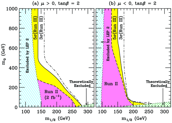
Figure 66: The contours of 99% C.L. observation at Run II and 5$\sigma$ discovery as well as 3$\sigma$ observation at Run III for $p\bar{p}\rightarrow{\rm SUSY\;\;particles}\rightarrow 3\ell+X$ with soft cuts A1, in the $(m_{1/2},m_{0})$ plane, for $\tan\beta=$ 2, (a) $\mu>0$ and (b) $\mu<0$.

Figure 67 shows the 99% C.L. observation contour of Run II and the $5\sigma$ discovery contour as well as the 3$\sigma$ observation contour of Run III for $p\bar{p}\rightarrow{\rm SUSY\;particles}\rightarrow 3\ell+X$ at $\sqrt{s}=2$ TeV with soft cuts A1, in the parameter space of $(m_{1/2},m_{0})$, for $\mu>0$, $\tan\beta=10$ and $\tan\beta=35$.

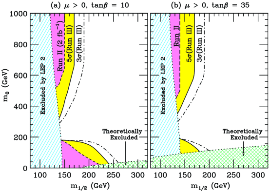
Figure 67: The same as Figure 66, for $\mu>0$, (a) $\tan\beta=$ 10 and (b) $\tan\beta=35$.

In Figure 68, we present the contours of 99% C.L. observation at Run II and $5\sigma$ discovery as well as 3$\sigma$ observation at Run III for $p\bar{p}\rightarrow{\rm SUSY\;Particles}\rightarrow 3\ell+X$ in the $(m_{1/2},m_{0})$ plane for $\tan\beta=3$ with soft cuts A1 and soft cuts A2.

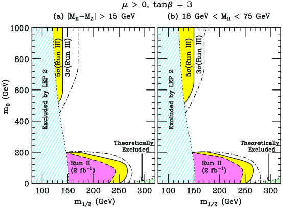
Figure 68: The same as Figure 66, for $\mu>0$ and $\tan\beta=3$, with (a) soft cuts A1 ($|M_{\ell\ell}-M_{Z}|>15$ GeV), and (b) soft cuts A2 ($M_{\ell\ell}<75$ GeV).

XXVI.4 Conclusions

In most of the mSUGRA parameter space, $\tilde{\chi}^{\pm}_{1}\tilde{\chi}^{0}_{2}$ production is the dominant source of trileptons. For $m_{0}\mathrel{\raisebox{-2.58334pt}{$\stackrel{{\scriptstyle\textstyle<}}{{\sim}}$}}150$ GeV and $\tan\beta\mathrel{\raisebox{-2.58334pt}{$\stackrel{{\scriptstyle\textstyle>}}{{\sim}}$}}20$, production of $\tilde{\ell}\tilde{\nu}$ and $\tilde{\ell}\tilde{\ell}$ can enhance the trilepton signal and may yield observable rates at Run III in regions of parameter space that are otherwise inaccessible. We summarize the contributions to trileptons from various channels for $\mu>0$ in Table 21.

Table 21: The cross section of $p\bar{p}\rightarrow{\rm SUSY\;\;particles}\rightarrow\break 3\ell+X$ in fb versus $\tan\beta$ with contributions from various relevant SUSY channels at $\sqrt{s}=2$ TeV with the acceptance cuts described in [Eqs. (193) and (194)] for $\mu>0$, $m_{1/2}=200$ GeV, $\tan\beta=3,10,20$ and 35 (25 for $m_{0}=100$ GeV).

Channel $\backslash\tan\beta$	3	10	20	35(25)
(i) $m_{0}=100$ GeV
Total	8.82	2.57	0.90	0.50
$\tilde{\chi}^{\pm}_{1}\tilde{\chi}^{0}_{2}$	7.16	1.74	0.40	0.13
$\tilde{\ell}\tilde{\nu}$	0.66	0.32	0.18	0.10
$\tilde{\ell}\tilde{\ell}$	0.33	0.16	0.15	0.13
$\tilde{\chi}^{0}_{2}\tilde{\chi}^{0}_{2}$, $\tilde{\chi}^{0}_{2}\tilde{\chi}^{0}_{3}$, $\tilde{\chi}^{0}_{3}\tilde{\chi}^{0}_{4}$,	0.30	0.12	0.05	0.05
$\tilde{\chi}^{\pm}_{1}\tilde{\chi}^{0}_{3,4}$, $\tilde{\chi}^{\pm}_{2}\tilde{\chi}^{0}_{3,4}$ $\tilde{\chi}^{\pm}_{1}\tilde{\chi}^{\mp}_{2}$, $\tilde{\chi}^{\pm}_{2}\tilde{\chi}^{\mp}_{2}$	0.07	0.08	0.06	0.05
$\tilde{g}\tilde{\chi}^{0}_{2,3}$, $\tilde{q}\tilde{\chi}^{0}_{2,3}$,$\tilde{g}\tilde{g}$, $\tilde{q}\tilde{q}$,$\tilde{\nu}\tilde{\nu}$	0.30	0.15	0.06	0.04
(ii) $m_{0}=200$ GeV
Total	1.07	0.23	0.25	0.31
$\tilde{\chi}^{\pm}_{1}\tilde{\chi}^{0}_{2}$	0.98	0.16	0.17	0.19
$\tilde{\ell}\tilde{\nu}$	0.03	0.02	0.02	0.03
$\tilde{\ell}\tilde{\ell}$	0.01	0.01	0.01	0.01
$\tilde{\chi}^{0}_{2}\tilde{\chi}^{0}_{2}$, $\tilde{\chi}^{0}_{2}\tilde{\chi}^{0}_{3}$, $\tilde{\chi}^{0}_{3}\tilde{\chi}^{0}_{4}$,	0.01	0.01	0.01	0.02
$\tilde{\chi}^{\pm}_{1}\tilde{\chi}^{0}_{3,4}$, $\tilde{\chi}^{\pm}_{2}\tilde{\chi}^{0}_{3,4}$ $\tilde{\chi}^{\pm}_{1}\tilde{\chi}^{\mp}_{2}$, $\tilde{\chi}^{\pm}_{2}\tilde{\chi}^{\mp}_{2}$	0.01	0.01	0.02	0.02
$\tilde{g}\tilde{\chi}^{0}_{2,3}$, $\tilde{q}\tilde{\chi}^{0}_{2,3}$,$\tilde{g}\tilde{g}$, $\tilde{q}\tilde{q}$,$\tilde{\nu}\tilde{\nu}$	0.03	0.02	0.02	0.04
(iii) $m_{0}=500$ GeV
Total	0.28	0.48	0.46	0.42
$\tilde{\chi}^{\pm}_{1}\tilde{\chi}^{0}_{2}$	0.28	0.45	0.44	0.41
$\tilde{\chi}^{0}_{2}\tilde{\chi}^{0}_{2}$, $\tilde{\chi}^{0}_{2}\tilde{\chi}^{0}_{3}$, $\tilde{\chi}^{0}_{3}\tilde{\chi}^{0}_{4}$,	$-$	0.01	$-$	$-$
$\tilde{\chi}^{\pm}_{1}\tilde{\chi}^{0}_{3,4}$, $\tilde{\chi}^{\pm}_{2}\tilde{\chi}^{0}_{3,4}$ $\tilde{\chi}^{\pm}_{1}\tilde{\chi}^{\mp}_{2}$, $\tilde{\chi}^{\pm}_{2}\tilde{\chi}^{\mp}_{2}$	$-$	0.01	0.01	$-$
$\tilde{g}\tilde{\chi}^{0}_{2,3}$, $\tilde{q}\tilde{\chi}^{0}_{2,3}$,$\tilde{g}\tilde{g}$, $\tilde{q}\tilde{q}$,$\tilde{\nu}\tilde{\nu}$	$-$	0.01	0.01	0.01

In regions of the parameter space with $m_{0}\mathrel{\raisebox{-2.58334pt}{$\stackrel{{\scriptstyle\textstyle<}}{{\sim}}$}}200$ GeV or $\tan\beta\mathrel{\raisebox{-2.58334pt}{$\stackrel{{\scriptstyle\textstyle>}}{{\sim}}$}}40$, the $\tilde{\chi}^{\pm}_{1}$ and the $\tilde{\chi}^{0}_{2}$ decay dominantly to final states with $\tau$ leptons. The subsequent leptonic decays of these $\tau$ leptons contribute importantly to the trilepton signal from $\tilde{\chi}^{\pm}_{1}\tilde{\chi}^{0}_{2}$ associated production. With soft but realistic lepton $p_{T}$ acceptance cuts, these $\tau\rightarrow\ell$ contributions can significantly enhance the trilepton signal. The Tevatron trilepton searches are most sensitive to the region of mSUGRA parameter space with $m_{0}\mathrel{\raisebox{-2.58334pt}{$\stackrel{{\scriptstyle\textstyle<}}{{\sim}}$}}100$ GeV and $\tan\beta\mathrel{\raisebox{-2.58334pt}{$\stackrel{{\scriptstyle\textstyle<}}{{\sim}}$}}$ 10.

The discovery potential of the upgraded Tevatron for $\mu>0$ are summarized in the following:

• For $m_{0}\sim 100$ GeV and $\tan\beta\sim 2$, the trilepton signal should be detectable at the Run II if $m_{1/2}\mathrel{\raisebox{-2.58334pt}{$\stackrel{{\scriptstyle\textstyle<}}{{\sim}}$}}$ 240 GeV ($m_{\tilde{\chi}^{\pm}_{1}}\mathrel{\raisebox{-2.58334pt}{$\stackrel{{\scriptstyle\textstyle<}}{{\sim}}$}}177$ GeV), and at the Run III if $m_{1/2}\mathrel{\raisebox{-2.58334pt}{$\stackrel{{\scriptstyle\textstyle<}}{{\sim}}$}}$ 260 GeV ($m_{\tilde{\chi}^{\pm}_{1}}\mathrel{\raisebox{-2.58334pt}{$\stackrel{{\scriptstyle\textstyle<}}{{\sim}}$}}195$ GeV).

• For $m_{0}\sim 150$ GeV and $\tan\beta\sim 35$, the trilepton signal should be detectable at the Run III if $m_{1/2}\mathrel{\raisebox{-2.58334pt}{$\stackrel{{\scriptstyle\textstyle<}}{{\sim}}$}}$ 170 GeV ($m_{\tilde{\chi}^{\pm}_{1}}\mathrel{\raisebox{-2.58334pt}{$\stackrel{{\scriptstyle\textstyle<}}{{\sim}}$}}122$ GeV).

• For $m_{0}\mathrel{\raisebox{-2.58334pt}{$\stackrel{{\scriptstyle\textstyle>}}{{\sim}}$}}600$ GeV and $\tan\beta\sim 35$, the trilepton signal should be detectable at the Run III if $m_{1/2}\mathrel{\raisebox{-2.58334pt}{$\stackrel{{\scriptstyle\textstyle<}}{{\sim}}$}}$ 170 GeV ($m_{\tilde{\chi}^{\pm}_{1}}\mathrel{\raisebox{-2.58334pt}{$\stackrel{{\scriptstyle\textstyle<}}{{\sim}}$}}130$ GeV).

For 180 GeV $\mathrel{\raisebox{-2.58334pt}{$\stackrel{{\scriptstyle\textstyle<}}{{\sim}}$}}m_{0}\mathrel{\raisebox{-2.58334pt}{$\stackrel{{\scriptstyle\textstyle<}}{{\sim}}$}}$ 350 GeV and $10\mathrel{\raisebox{-2.58334pt}{$\stackrel{{\scriptstyle\textstyle<}}{{\sim}}$}}\tan\beta\mathrel{\raisebox{-2.58334pt}{$\stackrel{{\scriptstyle\textstyle<}}{{\sim}}$}}35$, the $\tilde{\chi}^{0}_{2}$ decays dominantly into $q\bar{q}\tilde{\chi}^{0}_{1}$. In these regions it will be difficult to establish a trilepton signal. For $m_{0}\mathrel{\raisebox{-2.58334pt}{$\stackrel{{\scriptstyle\textstyle>}}{{\sim}}$}}$ 500 GeV and $m_{1/2}$ close to the reach of soft cuts, most trileptons from SUSY sources have relatively higher $p_{T}$ than those generated with lower $m_{0}$, and the statistical significance of the trilepton signal might be slightly improved by optimized harder cuts Matchev2 ; Baer&Tata . While there are regions of parameter space where it will be difficult to establish a trilepton signal because the leptonic decays of $\tilde{\chi}^{0}_{2}$ is suppressed, the important point is that the experiments at the Tevatron may probe a substantial region not accessible at LEP 2.

XXVI.5 Trilepton Analysis with Variable Cuts

In this section we summarize the results from a trilepton analysis with variable cuts MP3L-3l ; talks-3l ; MPPLB-3l . We perform a detailed Monte Carlo simulation of signal and background with a realistic detector simulation based on SHW v.2.2 SHW-a3l ; TAUOLA-a3l ; STDHEP-a3l . We used ISAJET ISAJET-3l for simulation of the signal, and PYTHIA PYTHIA-a3l for all background determinations except $WZ$. For $WZ$ we first use COMPHEP COMPHEP-a3l to generate hard scattering events at leading order, then we pipe those through PYTHIA, adding showering and hadronization, and finally, we run the resulting events through SHW. We made several modifications in the SHW/TAUOLA package, which are described in Refs. MP3L-3l ; MPPLB-3l . In our analysis we use several alternative values for the cut on a particular variable. 1) Four $\hbox to0.0pt{\,/\hss}E_{T}$ cuts: $\hbox to0.0pt{\,/\hss}E_{T}>\{15,20,25\}$ GeV or no cut. 2) Six high-end invariant mass cuts for any pair of opposite sign, same flavor leptons. The event is discarded if: $|M_{Z}-m_{\ell^{+}\ell^{-}}|<\{10,15\}$ GeV; or $m_{\ell^{+}\ell^{-}}>\{50,60,70,80\}$ GeV. 3) Eleven low-end invariant mass cuts for any pair of opposite sign, same flavor leptons: $m^{\gamma}_{\ell^{+}\ell^{-}}<\{10,60\}$ GeV, in 5 GeV increments. 4) Four azimuthal angle cuts on opposite sign, same flavor leptons: two cuts on the difference of the azimuthal angle of the two highest $p_{T}$ leptons, $|\Delta\varphi|<\{2.5,2.97\}$, one cut $|\Delta\varphi|<2.5$ for any pair leptons, and no cut. 5) An optional jet veto (JV) on QCD jets in the event. 6) An optional cut on the the transverse mass $m_{T}$ of any $\ell\nu$ pair which may originate from a $W$-boson: $60<m_{T}(\ell,\nu)<85$ GeV. 7) Five sets of lepton $p_{T}$ cuts: $\{11,5,5\},~{}\{11,7,5\},~{}\{11,7,7\},~{}\{11,11,11\}$ and $\{20,15,10\}$, where the first four sets also require a central lepton with $p_{T}>11$ GeV and $|\eta|<1.0$ or 1.5. We then employ a parameter space dependent cut optimization: at each point in SUSY parameter space, we consider all possible combinations of cuts, and determine the best combination by maximizing $S/\sqrt{B}$.

We present our results for the Tevatron reach in the trilepton channel in Figs. 69.

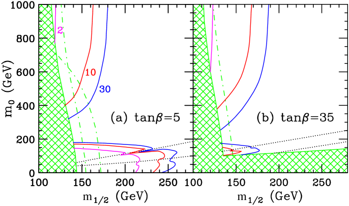
Figure 69: Tevatron reach in the trilepton channel in the $m_{0}-m_{1/2}$ plane, for fixed values of $A_{0}=0$, $\mu>0$ and (a) $\tan\beta=5$, or (b) $\tan\beta=35$. Results are shown for 2, 10 and 30 ${\rm fb}^{-1}$ total integrated luminosity.

We require the observation of at least 5 signal events, and present our results as $3\sigma$ exclusion contours in the $m_{0}-m_{1/2}$ plane, for two representative values of $\tan\beta$, 5 and 35. We fix $\mu>0$ and $A_{0}=0$. The cross-hatched region is excluded by current limits on the superpartner masses. The dot-dashed lines correspond to the projected LEP-II reach for the chargino and the lightest Higgs masses. In Fig. 69a the left dotted line shows where $m_{\tilde{\nu}_{\tau}}=m_{\tilde{\chi}_{1}^{\pm}}$ and the right dotted line indicates $m_{\tilde{\tau}_{1}}=m_{\tilde{\chi}_{1}^{\pm}}$ (and $m_{\tilde{\tau}}\simeq m_{\tilde{\mu}}\simeq m_{\tilde{e}}$). In Fig. 69b the dotted lines show where $m_{\tilde{e}_{R}}=m_{\tilde{\chi}_{1}^{\pm}}$ (left) and $m_{\tilde{\tau}_{1}}=m_{\tilde{\chi}_{1}^{\pm}}$ (right). We see that the trilepton channel provides for significant reach at both small $m_{0}$ ($m_{0}\lower 3.01385pt\hbox{$\;\stackrel{{\scriptstyle\textstyle<}}{{\sim}}\;$}150$ GeV) and large $m_{0}$ ($m_{0}\lower 3.01385pt\hbox{$\;\stackrel{{\scriptstyle\textstyle>}}{{\sim}}\;$}400$ GeV). With only 2 fb^-1 the reach is quite limited.

In Fig. 70 we show the optimum cuts chosen in our optimization procedure, in the $m_{0}$, $m_{1/2}$ plane, for $\tan\beta=5$, in the small $m_{0}$ region.

Figure 70: The optimal sets of trilepton cuts in the $m_{0},~{}m_{1/2}$ plane, for $\tan\beta=5$ and small $m_{0}$. We show the optimal low end dilepton mass cut $m^{\gamma}_{\ell^{+}\ell^{-}}$, missing $E_{T}$ cut $\hbox to0.0pt{\,/\hss}E_{T}$, high end dilepton mass cut $m_{\ell^{+}\ell^{-}}$, transverse $\ell\nu$ mass cut and lepton $p_{T}$ cut (see text). The dotted lines indicate the reach contours from Fig. 69. Note that the ranges of $m_{0}$ and $m_{1/2}$ are different from previous figures.

We use the following notation to describe the set of cuts at each point. The central symbol indicates the set of lepton $p_{T}$ cuts with higher values corresponding to harder cuts. The left superscript shows the value (in GeV) of the low-end invariant mass cut $m_{\ell^{+}\ell^{-}}^{\gamma}$. A left subscript “T” indicates that the cut on the transverse $\ell\nu$ mass was selected. The right superscript shows the $\hbox to0.0pt{\,/\hss}E_{T}$ cut: $\hbox to0.0pt{\,/\hss}E_{T}>\{15,20,25\}$ GeV (“15”,“20”,“25”), or no cut (no symbol). A right subscript denotes the high-end dilepton invariant mass cut: $|m_{\ell^{+}\ell^{-}}-M_{Z}|>\{10,15\}$ GeV (“10”,“15”) or $m_{\ell^{+}\ell^{-}}<\{50,60,70,80\}$ GeV (“50”,“60”,“70”,“80”). And finally, a tilde over the central symbol indicates that the luminosity limit came from requiring 5 signal events rather than $3\sigma$ exclusion. We see from Fig. 70 that in the regions where background is an issue, the combination of the $m_{T}$ cut and a tighter low-end dilepton mass cut $m^{\gamma}_{\ell^{+}\ell^{-}}\sim 20$ GeV is typically preferred. Notice that the transverse mass cut is never enough by itself, i.e. whenever it is chosen, it is almost always supplemented with a $m^{\gamma}_{\ell^{+}\ell^{-}}$ cut of 15 to 25 GeV (with the exception of two points with high lepton $p_{T}$ cuts). On the other hand, there are significant regions where the low invariant mass cut $m^{\gamma}_{\ell^{+}\ell^{-}}$ by itself is enough to kill the background, and the transverse mass cut is not needed.

XXVII Like-Sign Dilepton Analysis

The inclusive like-sign dilepton (2L) channel has been suggested JN-matchev as an alternative to the trilepton (3L) signature. By not requiring the odd-sign lepton in the event, the signal acceptance goes up, and the backgrounds are hopefully still under control.

In this section we summarize the results from a like-sign dilepton analysis with variable cuts MP3L-2l ; talks-2l ; MPPLB . We perform a detailed Monte Carlo simulation of signal and background with a realistic detector simulation based on SHW v.2.2 SHW-matchev ; TAUOLA ; STDHEP . We used ISAJET ISAJET-matchev for simulation of the signal, and PYTHIA PYTHIA-matchev for all background determinations except $WZ$. For $WZ$ we first use COMPHEP COMPHEP to generate hard scattering events at leading order, then we pipe those through PYTHIA, adding showering and hadronization, and finally, we run the resulting events through SHW. The resulting parton-level cross section was integrated with the CTEQ4m structure functions CTEQ-matchev . We have made several modifications in the SHW/TAUOLA package, which are appropriate for our purposes: 1) We modified TAUOLA to account for the correct (on average) polarization of tau leptons coming from decays of supersymmetric particles. 2) We extend the tracking coverage to $|\eta|<2.0$, which increases the electron and muon acceptance, as is expected in Run II TDR . For muons with $1.5<|\eta|<2.0$, we apply the same fiducial efficiency as for $1.0<|\eta|<1.5$. However, we still require that tau jets are reconstructed only up to $|\eta|<1.5$. 3) We retain the existing electron isolation requirement and add a muon isolation requirement $I<2$ GeV, where $I$ is the total transverse energy contained in a cone of size $\Delta R=\sqrt{\Delta\phi^{2}+\Delta\eta^{2}}=0.4$ around the muon. 4) We increase the jet cluster $E_{T}$ cut to 15 GeV and correct the jet energy for muons. We also add a simple electron/photon rejection cut $E_{em}/E_{had}<10$ to the jet reconstruction algorithm, where $E_{em}$ ($E_{had}$) is the cluster energy from the electromagnetic (hadronic) calorimeter. 5) We correct the calorimeter $\hbox to0.0pt{\,/\hss}E_{T}$ for muons. The addition of the muon isolation cut and the jet $E_{em}/E_{had}$ cut allows us to uniquely resolve the ambiguity arising in SHW v. 2.2, when a lepton and a jet are very close.

We conservatively use leading order cross sections for all processes, although NLO corrections should be incorporated in the experimental Run II analyses. Since the $k$-factor is roughly the same for both signal ino corr and background VV_corr ; tt_corr ; DY_corr , we expect that the Tevatron reach will be somewhat better once NLO corrections are accounted for.

In our analysis we use several alternative values for the cut on a particular variable. 1) Four $\hbox to0.0pt{\,/\hss}E_{T}$ cuts: $\hbox to0.0pt{\,/\hss}E_{T}>\{15,20,25\}$ GeV or no cut. 2) Six high-end invariant mass cuts for any pair of opposite sign, same flavor leptons. The event is discarded if: $|M_{Z}-m_{\ell^{+}\ell^{-}}|<\{10,15\}$ GeV; or $m_{\ell^{+}\ell^{-}}>\{50,60,70,80\}$ GeV. 3) Eleven low-end invariant mass cuts for any pair of opposite sign, same flavor leptons: $m^{\gamma}_{\ell^{+}\ell^{-}}<\{10,60\}$ GeV, in 5 GeV increments. 4) Four azimuthal angle cuts on opposite sign, same flavor leptons: two cuts on the difference of the azimuthal angle of the two highest $p_{T}$ leptons, $|\Delta\varphi|<\{2.5,2.97\}$, one cut $|\Delta\varphi|<2.5$ for any pair leptons, and no cut. 5) An optional jet veto (JV) on QCD jets in the event. 6) An optional cut on the the transverse mass $m_{T}$ of any $\ell\nu$ pair which may originate from a $W$-boson: $60<m_{T}(\ell,\nu)<85$ GeV. 7) Five sets of lepton $p_{T}$ cuts: $\{11,9\},~{}\{11,11\},~{}\{13,13\},~{}\{15,15\}$ and $\{20,20\}$. We then employ a parameter space dependent cut optimization: at each point in SUSY parameter space, we consider all possible combinations of cuts, and determine the best combination by maximizing $S/\sqrt{B}$.

We simulate the following background processes (with the generated number of events in parentheses): $ZZ$ ($10^{6}$), $WZ$ ($10^{6}$), $WW$ ($10^{6}$), $t\bar{t}$ ($10^{6}$), $Z+$jets ($8\cdot 10^{6}$) and $W+$jets ($8\cdot 10^{6}$).

A back-of-the-envelope comparison MP3L-2l of the $WZ$ backgrounds for the 3L and 2L channels reveals that vetoing the third lepton is not a good idea, so in what follows we only consider the inclusive 2L channel, just as in Ref. JN-matchev . In this case, the signal acceptance is definitely increased. Unfortunately, the corresponding increase in the background is even larger and the 2L channel is competitive with the 3L on the basis of $S/\sqrt{B}$ only if the lepton acceptance for the signal is less than $1/\sqrt{7.3}\sim 37\%$ MP3L-2l . However, for typical values of the SUSY model parameters the lepton acceptance is much higher and the 3L channel is preferred.

To make matters worse, the 2L channel suffers from a potentially large new source of background: $W+$jet production where the jet fakes a lepton. Although the rate for a jet faking a lepton is quite small, on the order of $10^{-4}$, the large $W+$jet cross section results in a major background for the 2L channel. The best way to estimate this background is from data, since Monte Carlo simulations are not reliable for fakes. In our analysis we shall follow the procedure of Ref. JN-matchev , where the rate for observing an isolated track which would otherwise pass the lepton cuts was measured in the Run I $Z+$jet event sample. This rate was then multiplied by the probability that, given an isolated track, it would fake a lepton. This probability was measured in Run I minimum bias events to be $\sim 1.5\%$, independent of $p_{T}$ JN-matchev . In our study we first simulate with Monte Carlo the $p_{T}$ distribution of isolated tracks in $W$ and $Z$ production. Then the 2L background cross section is obtained by multiplying the cross section for isolated tracks by the probability that an isolated track will fake a lepton. We normalize the isolated track rate to data. Using the measured 1.5% fake rate per isolated track, we find 1.5 fb of cross section when running the simulation at $\sqrt{s}=1800$ GeV and using the set of cuts from Ref. JN-matchev . This is half the cross section found in Ref. JN-matchev . Hence, to match the data to PYTHIA/SHW we need to double the isolated track rate obtained from Monte Carlo.

We present our results for the Tevatron reach in the like-sign dilepton channel in Fig. 71.

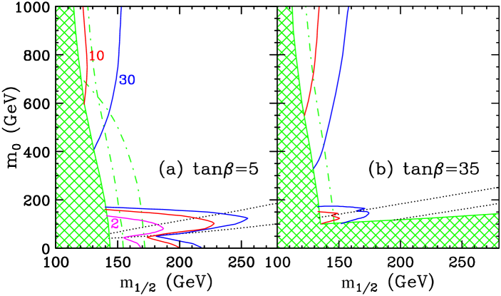
Figure 71: Tevatron reach in the like-sign dilepton channel in the $M_{0}-M_{1/2}$ plane, for fixed values of $A_{0}=0$, $\mu>0$ and (a) $\tan\beta=5$, or (b) $\tan\beta=35$. Results are shown for 2, 10 and 30 ${\rm fb}^{-1}$ total integrated luminosity.

We require the observation of at least 5 signal events, and present our results as $3\sigma$ exclusion contours in the $M_{0}-M_{1/2}$ plane, for two representative values of $\tan\beta$, 5 and 35. We fix $\mu>0$ and $A_{0}=0$. The cross-hatched region is excluded by current limits on the superpartner masses. The dot-dashed lines correspond to the projected LEP-II reach for the chargino and the lightest Higgs masses. In Fig. 71a the left dotted line shows where $m_{\tilde{\nu}_{\tau}}=m_{\tilde{\chi}_{1}^{\pm}}$ and the right dotted line indicates $m_{\tilde{\tau}_{1}}=m_{\tilde{\chi}_{1}^{\pm}}$ (and $m_{\tilde{\tau}}\simeq m_{\tilde{\mu}}\simeq m_{\tilde{e}}$). In Figs. 71b the dotted lines show where $m_{\tilde{e}_{R}}=m_{\tilde{\chi}_{1}^{\pm}}$ (left) and $m_{\tilde{\tau}_{1}}=m_{\tilde{\chi}_{1}^{\pm}}$ (right).

We see that the like-sign dilepton channel offers some reach at both small and large $M_{0}$, for both small and large values of $\tan\beta$. Based on the analysis presented here, the reach of the like-sign dilepton channel is not competitive with that of the clean trilepton channel3L-matchev .

XXVIII Study of a Like-Sign Dilepton Search for Chargino-Neutralino Production at CDF

XXVIII.1 Introduction

Previous searches for chargino-neutralino production at the Tevatron have focused primarily on signatures with three charged leptons (trileptons) plus missing transverse energy ($\raisebox{1.29167pt}{$\not$}E_{T}$) nacht-trilep . In the Minimal Supersymmetric (SUSY) Standard Model, chargino-neutralino production occurs in proton-antiproton (${p\bar{p}}$) collisions via a virtual $W$ ($s$ channel) or a virtual squark ($t$ channel). In a representative minimal Supergravity (SUGRA) model (parameters: $\mu<0,\tan\beta=2,{A_{0}}=0,m_{0}=200~{}{\rm GeV}/{\it c}^{2}$, $m_{1/2}=90-140~{}{\rm GeV}/{\it c}^{2}$), we expect three-body chargino and neutralino decays through virtual bosons and sleptons in a chargino mass region of $80-130~{}{\rm GeV}/{\it c}^{2}$. Conserving $R$-parity, these decays produce a distinct signature: trileptons plus $\raisebox{1.29167pt}{$\not$}E_{T}$ from a neutrino and the lightest supersymmetric particle. We demonstrate that the sensitivity to this signature can be significantly increased by searching for events with two like-sign leptons. The Like-Sign Dilepton (LSD) search provides a strong rejection of Standard Model background through the like-sign requirement, and enhances the acceptance of the signal by requiring only two of the three leptons produced in the chargino-neutralino decay.

XXVIII.2 Like-Sign Dilepton Analysis

Signal and most background processes were generated using ISAJET 7.20 and the CDF detector Monte Carlo simulation. For the signal estimation, we used representative SUGRA parameters of $\mu<0,\tan\beta=2,{A_{0}}=0,m_{0}=200~{}{\rm GeV}/{\it c}^{2}$, and $m_{1/2}=90-140~{}{\rm GeV}/{\it c}^{2}$. The relevant mass relations are ${M_{\tilde{\chi}_{1}^{\pm}}}\sim{M_{\tilde{\chi}_{2}^{0}}}\sim 2{M_{\tilde{\chi}_{1}^{0}}}$, with ${M_{\tilde{\chi}_{1}^{\pm}}}$ between $80-130~{}{\rm GeV}/{\it c}^{2}$. The sleptons and sneutrinos have masses between $200-220~{}{\rm GeV}/{\it c}^{2}$, so we generate only three-body chargino and neutralino decays.

The LSD analysis begins with the selection of a pair of leptons ($ee,\mu\mu,e\mu$) with the same charge. We then impose kinematic requirements on the selected events in order to remove Standard Model and other non-SUSY backgrounds. Our primary requirements are minimum transverse momentum ($P_{T}>11~{}{\rm GeV}/{\it c}$) for both leptons, and isolation, in which we remove events where at least one lepton has excess transverse energy greater than 2 GeV in a cone of 0.4 radians around the lepton. Monte Carlo simulations indicate that isolation removes heavy flavor (${b\bar{b}},{c\bar{c}}$) backgrounds most effectively. As the like-sign cut requires us to select both leptons from a $b$ or $c$ decay in such an event, and as semi-leptonic $b$ and $c$ decays produce leptons associated with jets, neither of the selected leptons will be isolated. Isolation also reduces ${t\bar{t}}$ background because at least one lepton from the like-sign pair will be selected from a $b$ decay in such an event. The isolation cut, when applied to both like-sign leptons, reduces ${b\bar{b}}$ and ${c\bar{c}}$ backgrounds to a negligible level.

We remove diboson events through a $Z$-mass rejection, in which the combined mass of a third opposite-sign, same-flavor lepton selected by the analysis and either of the LSDs is between 80–100 ${\rm GeV}/{\it c}^{2}$, reducing $WZ$ and $ZZ$ backgrounds. We impose no requirement on $\raisebox{1.29167pt}{$\not$}E_{T}$. This leaves $WZ$ production as the dominant source of Standard Model background, as shown in Table 22.

An important source of non-SUSY background estimated from data is events with one true lepton, such as W $\rightarrow\ell\nu$ + jets, and a “fake” lepton, i.e. an isolated track misidentified as a lepton. This fake lepton, in combination with the true lepton from the W decay, can be selected as a signal event in this analysis. In order to estimate this background, we first look at $Z\rightarrow{e^{+}e^{-}}$ + jets, which we assume provides a model for $W+\rm jets$ events. Removing the true leptons, we then measure the rate of underlying isolated tracks in the event. Next we search minimum bias data, in which we assume there are no true leptons, to find the probability of an isolated track to be misidentified as a lepton. The probability of misidentifying an isolated track as a lepton is 1.5$\%$ per track. We multiply this probability by the isolated track rate from the $Z$ $\rightarrow{e^{+}e^{-}}$ events, by the number of $W+\rm jets$ events expected run1w , and by a factor of 0.5 for the like-sign requirement. This “fake” rate drops rapidly with an increasing minimum $P_{T}$ requirement. Optimization of the number of expected background events as a function of the $P_{T}$ requirement yields 0.3 events expected from $W+\rm jets$ in 100 ${\rm pb}^{-1}$ of data.

XXVIII.3 Results

Applying the analysis requirements and normalizing the luminosity to 100 ${\rm pb}^{-1}$, the expected background is a total of 0.56 events, as shown in Table 22. Drell-Yan and $W+\rm jets$ are the most significant non-SUSY backgrounds; $WZ$ production is the largest Standard Model background. There is little background overlap of the trilepton and LSD analyses in the selected events based on Monte Carlo studies. Therefore, the backgrounds are treated as independent. For the trilepton analysis, the expected background for the Run I luminosity of 107 ${\rm pb}^{-1}$ is 1.2 events nacht-trilep . The total expected background for the combined LSD and trilepton analyses is 1.8 events.

Table 22: Background estimates for the number of events expected in 100 ${\rm pb}^{-1}$ of data based on Monte Carlo (except for the $W+\rm jets$ data estimation). The errors are one-sigma statistical errors.

Process	Luminosity(${\rm pb}^{-1}$)	${N_{events}}$ expected
$WZ$	16,684	$0.11\pm 0.02$
$ZZ$	13,992	$0.01\pm 0.01$
$WW$	6,870	$0^{+0.02}_{-0}$
${t\bar{t}}$	5,558	$0^{+0.02}_{-0}$
Drell-Yan($\gamma^{*}/Z$)	1,728	$0.11^{+0.10}_{-0.06}$
${{b\bar{b}},{c\bar{c}}}$	3,122	$0.03^{+0.04}_{-0.02}$
$W+\rm jets$	(from data)	0.30
Total		0.56

Figure 72 shows the efficiency versus chargino mass for the trilepton analysis, the LSD analysis, and the combined analyses, taking into account the signal overlap between the trilepton and LSD analyses. These efficiencies are calculated for all three analyses as number of selected events divided by total number of chargino-neutralino events where both sparticles decay leptonically, where a lepton can be $e,\mu,$ or $\tau$. All $\tau$ decays are included in this calculation, even though the analyses are only sensitive to the leptonic decays.

Figure 72: The efficiency (as the percentage of events selected) for the trilepton, LSD, and combined analyses as a function of chargino mass. SUGRA parameters of $\mu<0,\tan\beta=2,{A_{0}}=0,m_{0}=200~{}{\rm GeV}/{\it c}^{2}$, and $m_{1/2}=90-140~{}{\rm GeV}/{\it c}^{2}$ were used to measure the efficiency.

Figure 73 shows the average expected limit normalized to 100 ${\rm pb}^{-1}$ for the trilepton, LSD, and combined analyses. These limits were calculated from the efficiencies in Figure 72 and from the expected number of background events based on Monte Carlo.

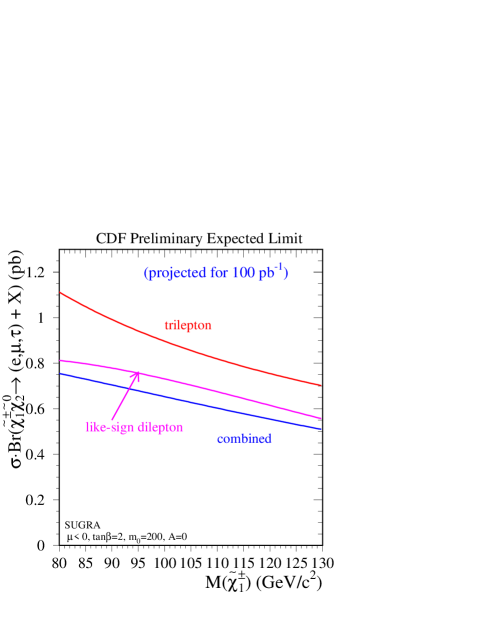
Figure 73: Average expected limit on $\sigma\cdot\cal{B}$ as a function of $M_{\tilde{\chi}_{1}^{\pm}}$ for the LSD analysis, trilepton analysis, and the combination of both analyses. The parametrized efficiencies shown in Figure 72 are used along with the expected background from Monte Carlo in this calculation.

XXVIII.4 Conclusion

This study indicates that a fully realized Like-Sign Dilepton analysis will increase the sensitivity of searches for chargino-neutralino production with the CDF detector using existing data of ${p\bar{p}}$ collisions at $\sqrt{s}=1.8$ TeV. It has been shown that the sensitivity of the previously published trilepton analysis can be improved by combining it with this new LSD signature search. Significantly, the LSD search has fewer requirements than the trilepton analysis, e.g. the trilepton analysis requires $\mbox{$\raisebox{1.29167pt}{$\not$}E_{T}$}>15~{}{\rm GeV}/{\it c}^{2}$ whereas the LSD analysis has no $\raisebox{1.29167pt}{$\not$}E_{T}$ requirement, making the Like-Sign Dilepton channel sensitive to a greater number of signatures.

XXIX Signatures with Tau Jets

XXIX.1 Introduction

Searches for supersymmetry (SUSY) in Run I of the Tevatron have been done exclusively in channels involving some combination of leptons, jets, photons and missing transverse energy ($\not\!\!\!E_{T}$) Tevatron searches . At the same time, several Run I analyses have identified hadronic tau jets, e.g. in $W$-production W to tau and top decays top to tau . Hadronically decaying taus have also been used to place limits on a charged Higgs H+ to tau and leptoquarks Leptoquark to tau . Since tau identification is expected to improve further in Run II, this raises the question whether SUSY searches in channels involving tau jets are feasible.

SUSY signatures with tau leptons are very well motivated, since they arise in a variety of models of low-energy supersymmetry, e.g. gravity mediated (SUGRA) BCDPT_PRL ; BCDPT_PRD ; JW or the minimal gauge-mediated models JW ; DN ; BT . Here we present results from a study LM of all possible experimental signatures with three identified objects (leptons or tau jets) plus $\not\!\!\!E_{T}$, and compare their reach to the clean trilepton channel Run I 3L ; 3L ; Barger ; BCDPT_PRL . In evaluating the physics potential of the future Tevatron runs in these new tau channels, it is important to be aware not only of the physical backgrounds, but also of the experimental realities. Jets faking taus will comprise a significant fraction of the background, and it is crucial to have a reliable estimate of that rate, which requires a detailed Monte Carlo analysis. We use PYTHIA PYTHIA and TAUOLA tauola for event generation, and the SHW package SHW , which provides a realistic detector simulation.

XXIX.2 Motivation

The classic signature for supersymmetry at the Tevatron is the clean $3\ell\,\not\!\!\!E_{T}$ channel. It arises in the decays of gaugino-like chargino-neutralino pairs $\tilde{\chi}^{\pm}_{1}\tilde{\chi}^{0}_{2}$. The reach is somewhat limited by the rather small leptonic branching fractions of the chargino and neutralino. In the limit of either heavy or mass degenerate squarks and sleptons, the leptonic branching ratios are $W$-like and $Z$-like, respectively. However, both gravity-mediated and gauge-mediated models of SUSY breaking allow the sleptons to be much lighter than the squarks, thus enhancing the leptonic branching fractions of the gauginos.

There are several generic reasons as to why one may expect light sleptons in the spectrum:

1. The slepton masses at the high-energy (GUT or messenger) scale may be rather small to begin with. This is typical for gauge-mediated models, since the sleptons are colorless and do not receive large soft mass contributions $\sim\alpha_{s}$. This argument applies to all slepton flavors, including staus. The minimal SUGRA models, on the other hand, predict light sleptons if $M_{0}\ll M_{1/2}$. Various effects (non-flat Kahler metric, RGE running above the GUT scale, D-terms from extra $U(1)$ gauge factors) may induce nonuniversalities in the scalar masses at the GUT scale, in which case the slepton-squark mass hierarchy can be affected. In the absence of a specific model, we do not know which way the splittings will go, but as long as the soft scalar masses are small, the RGE running down to the weak scale will naturally induce a splitting between the squarks and sleptons, making the sleptons lighter.

2. The renormalization group equations for the scalar soft masses contain terms proportional to Yukawa couplings, which tend to reduce the corresponding mass during the evolution down to low-energy scales. This effect is significant for third generation scalars, and for large values of $\tan\beta$ splits the staus from the first two generation sleptons.

3. The mixing in the charged slepton mass matrix further reduces the mass of the lightest eigenstate. The slepton mixing is enhanced at large $\tan\beta$, since it is proportional to $\mu m_{\ell}\tan\beta/m^{2}_{\tilde{\ell}}$, where $m_{\ell}$ ($m_{\tilde{\ell}}$) is the lepton (slepton) mass. Notice that this effect again only applies to the staus, since $m_{\tau}\gg m_{\mu,e}$.

Due to these effects, or some peculiar scalar mass non-universality, it may very well be that among all scalars, only the lightest sleptons from each generation (or maybe just the lightest stau $\tilde{\tau}_{1}$) are lighter than $\tilde{\chi}^{\pm}_{1}$ and $\tilde{\chi}^{0}_{2}$. Indeed, in both SUGRA and minimal gauge mediated models one readily finds regions of parameter space where either $m_{\tilde{\chi}^{0}_{1}}<m_{\tilde{\tau}_{1}}\sim m_{\tilde{\mu}_{R}}<m_{\tilde{\chi}^{+}_{1}}$ (typically at small $\tan\beta$) or $m_{\tilde{\chi}^{0}_{1}}<m_{\tilde{\tau}_{1}}<m_{\tilde{\chi}^{+}_{1}}<m_{\tilde{\mu}_{R}}$ (at large $\tan\beta$). Depending on the particular model, and the values of the parameters, the gaugino pair decay chain may then end up overwhelmingly in any one of the four final states: $\ell\ell\ell$, $\ell\ell\tau$, $\ell\tau\tau$ or $\tau\tau\tau$.

XXIX.2.1 Tau Jets

In order to make a final decision as to which experimental signatures are most promising, we have to factor in the tau branching ratios to leptons and jets. About two-thirds of the subsequent tau decays are hadronic, so it appears advantageous to consider signatures with tau jets in the final state as alternatives to the clean trilepton signal. The branching ratios for three leptons or undecayed taus into a final state containing leptons and tau jets is shown in Table 23. We see that the presence of taus in the underlying SUSY signal always leads to an enhancement of the signatures with tau jets in comparison to the clean trileptons. This disparity is most striking for the case of $\tau\tau\tau$ decays, where $BR(\tau\tau\tau\rightarrow\ell\ell\tau_{h})/BR(\tau\tau\tau\rightarrow\ell\ell\ell)\sim 5.5$.

Table 23: Branching ratios of the four possible SUSY signals into the corresponding experimental signatures involving final state leptons $l$ (electrons or muons) as well as identified tau jets ($\tau_{h}$).

Experimental	Trilepton SUSY signal
signature	$\tau\tau\tau$	$\tau\tau\ell$	$\tau\ell\ell$	$\ell\ell\ell$
$\tau_{h}\tau_{h}\tau_{h}$	0.268	—	—	—
$\ell\tau_{h}\tau_{h}$	0.443	0.416	—	—
$\ell\ell\tau_{h}$	0.244	0.458	0.645	—
$\ell\ell\ell$	0.045	0.126	0.355	1.00

An additional advantage of the tau jet channels is that the leptons from tau decays are much softer than the tau jets. In Fig. 74 we show the distribution of the $p_{T}$ fraction carried away by the visible decay products from the tau decay. We see that the lepton products are rather soft, so the benefit of reducing the corresponding $p_{T}$ cuts is an issue Barger .

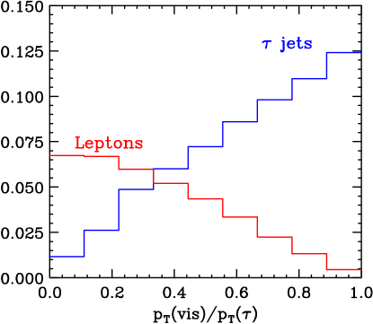
Figure 74: Distribution of the $p_{T}$ fraction that the visible tau decay products (charged leptons or tau jets) inherit from the tau parent.

It should be noted, however, that the tau jet channels suffer from larger backgrounds than the clean trileptons. The physical background (from real tau jets in the event) is actually smaller, but a significant part of the background is due to events containing narrow isolated QCD jets with the correct track multiplicity, which can be misidentified as taus. The jetty signatures are also hurt by the lower detector efficiency for tau jets than for leptons. The main goal of this study, therefore, will be to see what is the net effect of all these factors, on a channel by channel basis. We shall present the results from our Monte Carlo analysis in the next Section.

XXIX.2.2 A Challenging Scenario

For our analysis we choose to examine one of the most challenging scenarios for SUSY discovery at the Tevatron. We shall assume the typical large $\tan\beta$ mass hierarchy $m_{\tilde{\chi}^{0}_{1}}<m_{\tilde{\tau}_{1}}<m_{\tilde{\chi}^{+}_{1}}<m_{\tilde{\mu}_{R}}$. One then finds that $BR(\tilde{\chi}^{+}_{1}\tilde{\chi}^{0}_{2}\rightarrow\tau\tau\tau+X)\simeq 100\%$ below $\tilde{\chi}^{\pm}_{1}\rightarrow W^{\pm}\tilde{\chi}^{0}_{1}$ and $\tilde{\chi}^{0}_{2}\rightarrow Z\tilde{\chi}^{0}_{1}$ thresholds. (The region of gaugino masses where the two-body decays to gauge bosons are open is irrelevant for the Tevatron, as we shall see below.) In order to shy away from specific model dependence, we shall conservatively ignore all SUSY production channels other than $\tilde{\chi}^{\pm}_{1}\tilde{\chi}^{0}_{2}$ pair production. Production of any other supersymmetric particles, which can later decay into gauginos, will only enhance our signal.

The $p_{T}$ spectrum of the taus resulting from the chargino and neutralino decays depends on the mass differences $m_{\tilde{\chi}^{+}_{1}}-m_{\tilde{\tau}_{1}}$ and $m_{\tilde{\tau}_{1}}-m_{\tilde{\chi}^{0}_{1}}$. The larger they are, the harder the spectrum, and the better the detector efficiency. However, as the mass difference gets large, the $\tilde{\chi}^{+}_{1}$ and $\tilde{\chi}^{0}_{2}$ masses themselves become large, so the production cross-section is severely suppressed. Therefore, at the Tevatron we can only explore regions with favorable mass ratios and at the same time small enough gaugino masses. This suggests a choice of SUSY mass ratios for this study: for definiteness we fix $2m_{\tilde{\chi}^{0}_{1}}\sim(4/3)\ m_{\tilde{\tau}_{1}}\sim m_{\tilde{\chi}^{+}_{1}}(<m_{\tilde{\mu}_{R}})$ throughout the analysis, and vary the chargino mass. The rest of the parameters (first two generation slepton, heavier stau, tau sneutrino, squark, gluino, Higgs and higgsino masses) have constant values corresponding to the SUGRA point $M_{0}=180$ GeV, $M_{1/2}=180$ GeV, $A_{0}=0$ GeV, $\tan\beta=44$ and $\mu>0$, but we are not constrained to SUGRA models only. Our analysis will apply equally to gauge-mediated models with a long-lived neutralino NLSP, as long as the relevant gaugino and slepton mass relations are similar. Note that our choice of heavy first two generation sleptons is very conservative. A more judicious choice of their masses, namely $m_{\tilde{\mu}_{R}}<m_{\tilde{\chi}^{+}_{1}}$, would lead to a larger fraction of trilepton events, and as a result, a higher reach. Furthermore, the gauginos would then decay via two-body modes to first generation sleptons, and the resulting lepton spectrum would be much harder, leading to a higher lepton efficiency. With our choice of the superpartner spectrum, all two-body gaugino decays to first two generation sleptons are closed, which diminishes the discovery reach of the trilepton channel.

Since the four experimental signatures in our analysis contain only soft leptons and tau jets, an important issue is whether one can develop efficient combinations of Level 1 and Level 2 triggers to accumulate these data sets without squandering all of the available bandwidth. We will not attempt to address this issue in detail here; instead we will assume 100% trigger efficiency for those signal events which pass all of our analysis and acceptance cuts. We have nevertheless studied the following set of triggers BCDPT_PRD : 1) $\not\!\!\!E_{T}>40$ GeV; 2) $p_{T}(\ell)>20$ GeV and 3) $p_{T}(\ell)>10$ GeV, $p_{T}({\rm jet})>15$ GeV and $\not\!\!\!E_{T}>15$ GeV; with pseudorapidity cuts $|\eta(e)|<2.0$, $|\eta(\mu)|<1.5$ and $|\eta(jet)|<4.0$. We found that they are efficient in picking out about 90 % of the signal events in the channels with at least one lepton (see below). Dedicated low $p_{T}$ tau triggers for Run II, which may be suitable for the new tau jet channels, are now being considered by both CDF CDF tau trigger and D0 D0 tau trigger .

XXIX.3 Analysis

We used PYTHIA v6.115 and TAUOLA v2.5 for event generation. We used the SHW v2.2 detector simulation package, which simulates an average of the CDF and D0 Run II detector performance. In SHW tau objects are defined as jets with $|\eta|<1.5$, net charge $\pm 1$, one or three tracks in a $10$ degree cone with no additional tracks in a $30$ degree cone, $E_{T}>5$ GeV, $p_{T}>5$ GeV, plus an electron rejection cut. SHW electrons are required to have $|\eta|<1.5$, $E_{T}>5$ GeV, hadronic to electromagnetic energy deposit ratio $R_{h/e}<0.125$, and satisfy standard isolation cuts. Muon objects are required to have $|\eta|<1.5$, $E_{T}>3$ GeV and are reconstructed using the expected Run II muon detection efficiencies. We use standard isolation cuts for muons as well. Jets are required to have $|\eta|<4$ and $E_{T}>15$ GeV. In addition we have added jet energy correction for muons and the rather loose jet id requirement $R_{h/e}>0.1$. We have also modified the TAUOLA program in order to correctly account for the chirality of tau leptons coming from SUSY decays.

The reconstruction algorithms in SHW already include some basic cuts, so we can define a reconstruction efficiency $\epsilon_{rec}$ for the various types of objects: electrons, muons, tau jets etc. We find that as we vary the chargino mass from 100 to 140 GeV the electron and tau jet reconstruction efficiencies range from 42 to 49 %, and from 29 to 36%, correspondingly. The lepton efficiency may seem surprisingly low, but this is because a lot of our leptons are very soft and fail the $E_{T}$ cut. The tau efficiency is in good agreement with the results from Ref. CDF thesis and Leslie , once we account for the different cuts used in those analyses.

The most important issue in these channels is the fake tau rate. Several experimental analyses try to estimate it using Run I data. Here we simulate the corresponding backgrounds to our signal and use SHW to obtain the fake rate, thus avoiding trigger bias CDF thesis . We find that the SHW tau fake rate in $W$ production is roughly 1.5%, and almost independent of the tau $p_{T}$.

XXIX.3.1 Cuts

As discussed earlier, we expect that the reach in the classic $\ell\ell\ell\not\!\!\!E_{T}$ channel will be quite suppressed, due to the softness of the leptons. Therefore we apply the soft cuts proposed in Refs. Barger . We require a central lepton with $p_{T}>11$ GeV and $|\eta|<1.0$, and in addition two more leptons with $p_{T}(\ell_{2})>7$ GeV and $p_{T}(\ell_{3})>5$ GeV. Leptons are required to be isolated: $I(\ell)<2$ GeV, where $I$ is the total transverse energy contained in a cone of size $\delta R=\sqrt{\Delta\phi^{2}+\Delta\eta^{2}}=0.4$ around the lepton. We impose a dilepton invariant mass cut for same flavor, opposite sign leptons: $|m_{\ell\ell}-M_{Z}|>10$ GeV and $|m_{\ell\ell}|>11$ GeV. Finally, we impose an optional veto on additional jets with $p_{T}>15$ GeV, and require $\not\!\!\!E_{T}$ to be either more than 20 GeV, or 25 GeV. This gives us a total of four combinations of the $\not\!\!\!E_{T}$ cut and the jet veto (shown in Table. 24), which we apply for all tau jet signatures later as well.

Table 24: Definition of the signal samples A-D.

Sample	$\not\!\!\!E_{T}$ cut	Jet veto
A	20 GeV	no
B	25 GeV	no
C	20 GeV	yes
D	25 GeV	yes

For our $\ell\ell\tau_{h}\not\!\!E_{T}$ analysis we impose cuts similar to the stop search analysis in the $\ell^{+}\ell^{-}j\!\not\!\!\!E_{T}$ channel CDFanalysis : two isolated ($I(\ell)<2$ GeV) leptons with $p_{T}(\ell_{1})>8$ GeV and $p_{T}(\ell_{2})>5$ GeV and one identified hadronic tau jet with $p_{T}(\tau_{h})>15$ GeV. Again, we impose invariant mass cuts $|m_{\ell\ell}-m_{Z}|>10$ GeV and $|m_{\ell\ell}|>11$ for any same flavor, opposite sign dilepton pair.

A separate, very interesting signature arises if the two leptons have the same sign, since the background is greatly suppressed. In fact, we expect this background to be significantly smaller than the trilepton background! Roughly one third of the signal events in the general $\ell\ell\tau_{h}$ sample are expected to have like-sign leptons.

For our $\ell\tau_{h}\tau_{h}\not\!\!E_{T}$ analysis we use some basic identification cuts: two tau jets with $p_{T}>15$ GeV and $p_{T}>10$ GeV and one isolated lepton with $p_{T}(\ell)>7$ GeV.

Finally, for the $\tau_{h}\tau_{h}\tau_{h}\not\!\!E_{T}$ signature we require three tau jets with $p_{T}>15$ GeV, $p_{T}>10$ GeV and $p_{T}(\tau_{3})>8$ GeV, respectively.

XXIX.3.2 Signal

One can get a good idea of the relative importance of the different channels by looking at the corresponding signal samples after the analysis cuts have been applied. In Fig. 75 we show the signal cross-sections times the corresponding branching ratios times the total efficiency $\epsilon_{tot}\equiv\epsilon_{rec}\epsilon_{cuts}$, which accounts for both the detector acceptance and the efficiency of the cuts (for each point we generated 100,000 signal events).

Figure 75: Signal cross-section times branching ratio after cuts for the five channels discussed in the text: $\ell\ell\ell\not\!\!\!E_{T}$ (dotted), $\ell\ell\tau_{h}\not\!\!\!E_{T}$ (dashed), $\ell^{+}\ell^{+}\tau_{h}\not\!\!\!E_{T}$ (dot dashed), $\ell\tau_{h}\tau_{h}\not\!\!\!E_{T}$ (dot dot dashed) and $\tau_{h}\tau_{h}\tau_{h}\not\!\!\!E_{T}$ (solid); and for the four signal samples from Table 24: a) A, b) B, c) C and d) D.

We see that the lines are roughly ordered according to the branching ratios from Table 23. This can be understood as follows. The acceptance (which includes the basic ID cuts in SHW) is higher for leptons than for $\tau$ jets. Therefore, replacing a lepton with a tau jet in the experimental signature costs us a factor of $\sim 1.5$ in acceptance, due to the poorer reconstruction of tau jets, compared to leptons. Later, however, the cuts tend to reduce the leptonic signal more than the tau jet signal. This is mostly because the leptons are softer than the tau jets. Notice that we cannot improve the efficiency for leptons by further lowering the cuts – we are already using the most liberal cuts Barger . It turns out that these two effects mostly cancel each other, and the total efficiency $\epsilon_{tot}$ is roughly the same for all channels. Therefore the relative importance of each channel will only depend on the tau branching ratios and the backgrounds. For example, in going from $\ell\ell\ell$ to $\ell\ell\tau_{h}$, one wins a factor of 5.5 from the branching ratio. Therefore the background to $\ell\tau_{h}\tau_{h}\not\!\!\!E_{T}$ must be at least $5.5^{2}\sim 30$ times larger in order for the clean trilepton channel to be still preferred.

XXIX.3.3 Backgrounds

We next turn to the discussion of the backgrounds involved. We have simulated the following physics background processes: $ZZ$, $WZ$, $WW$, $t\bar{t}$, $Z+jets$, and $W+jets$, generating $4\times(10^{6})$ and $2\times(10^{7})$ events, respectively. We list the results in Tables 25-28, where all errors are purely statistical.

A number of interesting observations can be made regarding these backgrounds:

1. $WZ$ is indeed the major source of background for the trilepton channel. The majority of the background events contain a leptonically decaying off-shell $Z$ and pass the invariant dilepton mass cut. The rest of the WZ background comes from $Z\rightarrow\tau^{+}\tau^{-}\rightarrow\ell^{+}\ell^{-}\not\!\!\!E_{T}$. We find a total $WZ$ rate which is a factor of three higher than in recent trilepton analyses prior to this workshop (see, e.g. BCDPT_PRL , BCDPT_PRD , Barger ). To simulate the diboson backgrounds, these previous estimates employed ISAJET, where the $W$ and $Z$ gauge bosons are always generated exactly on their mass shell, and there is no finite-width smearing effect MP_comp , MP_PRD .

2. As we move to channels with more tau jets, the number of background events with real tau jets decreases: first, because of the smaller branching ratios of $W$ and $Z$ to taus; and second, because the tau jets in $W$ and $Z$ decays are softer than the leptons from $W$ and $Z$. This is to be contrasted with the signal, where, conversely, the tau jets are harder than the leptons. We also see, however, that the contribution from events with fake taus (from hadronically decaying $W$’s and $Z$’s or from initial and final state jet radiation) increases, and for the $3\tau$ channel events with fake taus are the dominant part of the $WZ$ background.

3. Notice that the $WZ$ background to the same-sign dilepton channel is smaller (by a factor of two) than for the trilepton channel. As expected, it is also about a half of the total contribution to $\ell\ell\tau$ (recall that for the signal this ratio is only a third). Indeed, one third of the events with opposite sign leptons come from the $Z$-decay and are cut away by the dilepton mass cut.

4. Vetoing a fourth lepton in the event reduces the $ZZ$ background to the trilepton channel only by 4–8 %. The $ZZ$ trilepton background is due to one $Z$ decaying as $Z\rightarrow\tau\tau$, thus providing the missing energy in the event, and the other $Z$ decaying to leptons: $Z\rightarrow\ell^{+}\ell^{-}$. Most of the events passing the cuts contain an off-shell $Z/\gamma$ decaying leptonically, and the third lepton coming from a leptonic tau. But then it is 6 times more probable that the second tau would decay hadronically and will not give a fourth lepton. The rest of the $ZZ$ background events come from a regular $Z\rightarrow\ell^{+}\ell^{-}$ decay, where one of the leptons is missed, and the invariant mass cut does not apply. For those events, there is obviously no fourth lepton.

5. The jet veto is very effective in reducing the $t\bar{t}$ background for the first three channels. However, it also reduces the signal (see Fig. 75).

6. In all channels, a higher $\not\!\!\!E_{T}$ cut did not help to get rid of the major backgrounds. Indeed, $WZ$, $t\bar{t}$ and/or $W+jets$ backgrounds tend to have a lot of missing energy, due to the leptonic W-decays.

7. Our result for the $W+jets$ and $Z+jets$ backgrounds should be taken with a grain of salt, in spite of the relatively small statistical errors. Events with fake leptons are expected to comprise a major part of this background, and SHW does not provide a realistic simulation of those. In fact, the most reliable way to estimate this background will be from Run IIa data, e.g. by estimating the probability for an isolated track from Drell-Yan events, and the lepton fake rate per isolated track from minimum bias data JN ; MP_PRD ; MP_PLB .

8. We have underestimated the total background to the three-jet channel by considering only processes with at least one real tau in the event. We expect sizable contributions from pure QCD multijet events, or $Wj\rightarrow jjj$, where all three tau jets are fake.

Table 25: Results for the backgrounds in the various channels in case A: $\not\!\!\!E_{T}>20$ GeV and no jet veto.

Case A: $\not\!\!\!E_{T}>20$	Experimental signatures
	$\ell\ell\ell\!\!\not\!\!\!E_{T}$	$\ell\ell\tau_{h}\!\!\not\!\!\!E_{T}$	$\ell^{+}\ell^{+}\tau_{h}\!\!\not\!\!\!E_{T}$	$\ell\tau_{h}\tau_{h}\!\!\not\!\!\!E_{T}$	$\tau_{h}\tau_{h}\tau_{h}\!\!\not\!\!\!E_{T}$
$ZZ$	0.196 $\pm$ 0.028	0.334 $\pm$ 0.036	0.094 $\pm$ 0.019	0.181 $\pm$ 0.027	0.098 $\pm$ 0.020
$WZ$ (fb)	1.058 $\pm$ 0.052	1.087 $\pm$ 0.053	0.447 $\pm$ 0.034	1.006 $\pm$ 0.051	0.248 $\pm$ 0.025
$WW$ (fb)	—	0.416 $\pm$ 0.061	—	0.681 $\pm$ 0.078	0.177 $\pm$ 0.039
$t\bar{t}$ (fb)	0.300 $\pm$ 0.057	1.543 $\pm$ 0.128	0.139 $\pm$ 0.038	1.039 $\pm$ 0.105	0.161 $\pm$ 0.041
$Z+jets$ (fb)	0.112 $\pm$ 0.079	7.34 $\pm$ 0.64	0.168 $\pm$ 0.097	20.3 $\pm$ 1.1	17.9 $\pm$ 1.0
$W+jets$ (fb)	—	—	—	37.2 $\pm$ 2.9	6.1 $\pm$ 1.2
$\sigma_{BG}^{\rm tot}$ (fb)	1.67 $\pm$ 0.11	10.7 $\pm$ 0.7	0.85 $\pm$ 0.11	60.4 $\pm$ 3.1	24.7 $\pm$ 1.6

Table 26: Results for the backgrounds in the various channels in case B: $\not\!\!\!E_{T}>25$ GeV and no jet veto.

Case B: $\not\!\!\!E_{T}>25$	Experimental signatures
	$\ell\ell\ell\!\!\not\!\!\!E_{T}$	$\ell\ell\tau_{h}\!\!\not\!\!\!E_{T}$	$\ell^{+}\ell^{+}\tau_{h}\!\!\not\!\!\!E_{T}$	$\ell\tau_{h}\tau_{h}\!\!\not\!\!\!E_{T}$	$\tau_{h}\tau_{h}\tau_{h}\!\!\not\!\!\!E_{T}$
$ZZ$ (fb)	0.165 $\pm$ 0.025	0.271 $\pm$ 0.033	0.090 $\pm$ 0.019	0.153 $\pm$ 0.024	0.086 $\pm$ 0.018
$WZ$ (fb)	0.964 $\pm$ 0.050	1.001 $\pm$ 0.051	0.423 $\pm$ 0.033	0.909 $\pm$ 0.049	0.204 $\pm$ 0.023
$WW$ (fb)	—	0.380 $\pm$ 0.058	—	0.602 $\pm$ 0.073	0.142 $\pm$ 0.036
$t\bar{t}$ (fb)	0.300 $\pm$ 0.057	1.500 $\pm$ 0.127	0.139 $\pm$ 0.038	0.996 $\pm$ 0.103	0.128 $\pm$ 0.037
$Z+jets$ (fb)	0.056 $\pm$ 0.056	4.87 $\pm$ 0.52	0.112 $\pm$ 0.079	13.61 $\pm$ 0.87	11.82 $\pm$ 0.81
$W+jets$ (fb)	—	—	—	32.1 $\pm$ 2.7	5.5 $\pm$ 1.1
$\sigma_{BG}^{\rm tot}$ (fb)	1.49 $\pm$ 0.10	8.0 $\pm$ 0.5	0.76 $\pm$ 0.09	48.4 $\pm$ 2.8	17.9 $\pm$ 1.4

Table 27: Results for the backgrounds in the various channels in case C: $\not\!\!\!E_{T}>20$ GeV and no extra jets with $p_{T}>15$ GeV.

Case C: $\not\!\!\!E_{T}>20$	Experimental signatures
jet veto	$\ell\ell\ell\!\!\not\!\!\!E_{T}$	$\ell\ell\tau_{h}\!\!\not\!\!\!E_{T}$	$\ell^{+}\ell^{+}\tau_{h}\!\!\not\!\!\!E_{T}$	$\ell\tau_{h}\tau_{h}\!\!\not\!\!\!E_{T}$	$\tau_{h}\tau_{h}\tau_{h}\!\!\not\!\!\!E_{T}$
$ZZ$ (fb)	0.114 $\pm$ 0.021	0.220 $\pm$ 0.029	0.071 $\pm$ 0.017	0.094 $\pm$ 0.019	0.031 $\pm$ 0.011
$WZ$ (fb)	0.805 $\pm$ 0.046	0.828 $\pm$ 0.046	0.347 $\pm$ 0.030	0.695 $\pm$ 0.043	0.136 $\pm$ 0.019
$WW$ (fb)	—	0.301 $\pm$ 0.052	—	0.354 $\pm$ 0.056	0.097 $\pm$ 0.029
$t\bar{t}$ (fb)	—	0.086 $\pm$ 0.030	—	0.032 $\pm$ 0.018	—
$Z+jets$ (fb)	0.056 $\pm$ 0.056	4.93 $\pm$ 0.52	0.056 $\pm$ 0.056	12.66 $\pm$ 0.84	10.36 $\pm$ 0.76
$W+jets$ (fb)	—	—	—	25.8 $\pm$ 2.4	3.2 $\pm$ 0.9
$\sigma_{BG}^{\rm tot}$ (fb)	0.97 $\pm$ 0.07	6.4 $\pm$ 0.5	0.47 $\pm$ 0.06	39.6 $\pm$ 2.5	13.8 $\pm$ 1.2

Table 28: Results for the backgrounds in the various channels in case D: $\not\!\!\!E_{T}>25$ GeV and no extra jets with $p_{T}>15$ GeV.

Case D: $\not\!\!\!E_{T}>25$	Experimental signatures
jet veto	$\ell\ell\ell\!\!\not\!\!\!E_{T}$	$\ell\ell\tau_{h}\!\!\not\!\!\!E_{T}$	$\ell^{+}\ell^{+}\tau_{h}\!\!\not\!\!\!E_{T}$	$\ell\tau_{h}\tau_{h}\!\!\not\!\!\!E_{T}$	$\tau_{h}\tau_{h}\tau_{h}\!\!\not\!\!\!E_{T}$
$ZZ$ (fb)	0.098 $\pm$ 0.020	0.177 $\pm$ 0.026	0.071 $\pm$ 0.017	0.075 $\pm$ 0.017	0.027 $\pm$ 0.010
$WZ$ (fb)	0.732 $\pm$ 0.044	0.766 $\pm$ 0.045	0.329 $\pm$ 0.029	0.622 $\pm$ 0.040	0.115 $\pm$ 0.017
$WW$ (fb)	—	0.274 $\pm$ 0.049	—	0.327 $\pm$ 0.054	0.071 $\pm$ 0.025
$t\bar{t}$ (fb)	—	0.075 $\pm$ 0.028	—	0.032 $\pm$ 0.018	—
$Z+jets$ (fb)	—	3.25 $\pm$ 0.24	—	7.62 $\pm$ 0.65	6.55 $\pm$ 0.61
$W+jets$ (fb)	—	—	—	22.6 $\pm$ 2.3	3.0 $\pm$ 0.8
$\sigma_{BG}^{\rm tot}$ (fb)	0.83 $\pm$ 0.05	4.5 $\pm$ 0.3	0.40 $\pm$ 0.03	31.3 $\pm$ 2.4	9.8 $\pm$ 1.0

XXIX.3.4 Tevatron reach

We are now ready to present our results for the Tevatron reach in Run II. A $3\sigma$ exclusion limit would require

$$L\ =\ {9\sigma_{BG}\over\left(\sigma\times BR(\tilde{\chi}^{+}_{1}\tilde{\chi}^{0}_{2}\rightarrow X)\epsilon_{tot}\right)^{2}}.$$ (195)

Notice that the limit depends linearly on the background $\sigma_{BG}$ after cuts, but quadratically on the signal branching ratios. This allows the jetty channels to compete very successfully with the clean trilepton signature, whose branching ratio is quite small.

Figure 76: The total integrated luminosity $L$ needed for a $3\sigma$ exclusion (solid lines) or observation of 5 signal events (dashed lines), as a function of the chargino mass $m_{\tilde{\chi}^{+}_{1}}$, for (a) sample A; (b) sample B; (c) sample C and (d) sample D, as defined in Table 24; and for the following channels: trileptons ($\times$), dileptons plus a tau jet ($\Box$) and like-sign dileptons plus a tau jet ($\Diamond$).

In Fig. 76 we show the Tevatron reach in the three channels: trileptons ($\times$), dileptons plus a tau jet ($\Box$) and like-sign dileptons plus a tau jet ($\Diamond$). We see that the two channels with tau jets have a much better sensitivity compared to the usual trilepton signature. Assuming that efficient triggers can be implemented, the Tevatron reach will start exceeding LEP II limits as soon as Run IIa is completed and the two collaborations have collected a total of $4\ {\rm fb}^{-1}$ of data. Considering the intrinsic difficulty of the SUSY scenario we are contemplating, the mass reach for Run IIb is quite impressive. One should also keep in mind that we did not attempt to optimize our cuts for the new channels. For example, one could use angular correlation cuts to suppress Drell-Yan, transverse $W$ mass cut to suppress $WZ$ BDPQT , or (chargino) mass–dependent $p_{T}$ cuts for the leptons and tau jets MP_PRD ; MP_PLB , to squeeze out some extra reach. In addition, the $ll\tau_{h}$ channel can be explored at smaller values of $\tan\beta$ as well BCDPT_PRD ; Barger ; MP_PRD ; MP_PLB (see also the section on trileptons, dileptons and dileptons plus tau jets in this Report), since the two-body chargino decays are preferentially to tau sleptons. In that case, the clean trilepton channel still offers the best reach, and a signal can be observed already in Run IIa. Then, the tau channels will not only provide an important confirmation, but also hint towards some probable values of the SUSY model parameters.

XXIX.4 Dilepton Plus Tau Jet Analysis with Variable Cuts

Subsequently, the dilepton plus tau jet channel was analysed again in Refs. MP_PRD ; MP_PLB . The main improvements were the inclusion of the $\gamma^{\ast}$ contribution of the $WZ$ background, and parameter space dependent cut optimization. For details on the numerical procedure, see Refs. MP_PRD ; MP_PLB and the like-sign dilepton section in this report.

The results for the Tevatron reach in the dilepton plus tau jet channel are shown in Fig. 77. We require the observation of at least 5 signal events, and present the results as $3\sigma$ exclusion contours in the $M_{0}-M_{1/2}$ plane, for two representative values of $\tan\beta$, 5 and 35. We fix $\mu>0$ and $A_{0}=0$. The cross-hatched region is excluded by current limits on the superpartner masses. The dot-dashed lines correspond to the projected LEP-II reach for the chargino and the lightest Higgs masses. In Fig. 77a the left dotted line shows where $m_{\tilde{\nu}_{\tau}}=m_{\tilde{\chi}_{1}^{\pm}}$ and the right dotted line indicates $m_{\tilde{\tau}_{1}}=m_{\tilde{\chi}_{1}^{\pm}}$ (and $m_{\tilde{\tau}}\simeq m_{\tilde{\mu}}\simeq m_{\tilde{e}}$). In Fig. 77b the dotted lines show where $m_{\tilde{e}_{R}}=m_{\tilde{\chi}_{1}^{\pm}}$ (left) and $m_{\tilde{\tau}_{1}}=m_{\tilde{\chi}_{1}^{\pm}}$ (right). We see that the dilepton plus tau jet channel provides some reach, but only at small $M_{0}$.

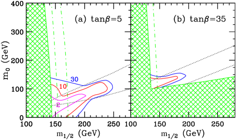
Figure 77: Tevatron reach in the dilepton plus tau jet channel in the $M_{0}-M_{1/2}$ plane, for fixed values of $A_{0}=0$, $\mu>0$ and (a) $\tan\beta=5$, or (b) $\tan\beta=35$. Results are shown for 2, 10 and 30 ${\rm fb}^{-1}$ total integrated luminosity.

XXX Implications of Non-Universal Gaugino Masses for Tevatron SUSY Searches

XXX.1 Non-universality of soft SUSY breaking terms

A crucial assumption underlying the mSUGRA framework is that the soft supersymmetry breaking gaugino masses, scalar masses and trilinear ($A$) terms are universal at the unification scale. This is, however, only an assumption— guided by phenomenological considerations such as the non-observation of neutral currents— about the symmetries of physics at high scales. Without such a symmetry, quantum corrections to soft SUSY breaking terms can break their degeneracybagger and universality fails. In fact, neither gauginos nor scalars are required to have universal masses in supergravity modelsearly . Indeed, there are many scenarios with non-universal soft supersymmetry breaking terms at the $GUT$ scale. These include:

• models with universality at the Planck or string scales. RGE evolution between $M_{Planck}$ or $M_{String}$ and $M_{GUT}\simeq 2\times 10^{16}$ GeV then leads to non-universalitypp .

• Various superstring models can lead to non-universality in soft SUSY breaking termsibanez ; cdg .

• If hidden sector fields whose vevs break SUSY live in higher dimensional GUT representations, then specific patterns of non-universality can be achievedsnowmass ; nonu-abct .

• Large Yukawa couplings can lead to non-universality of mainly third generation scalar masseshall .

In this section, we investigate the consequences of the fourth item above for SUSY searches at the Fermilab Tevatron collider and its upgrade options.

If one views the mSUGRA model in the context of $SU(5)$ grand unification, then it can be assumed that SUSY breaking occurs in the hidden sector via the development of a vacuum expectation value (vev) by the auxiliary component of an $SU(5)$ singlet superfield $\hat{\Phi}$. However, $SU(5)$ SUGRA grand unified (GUT) models can also be constructedsnowmass ; nonu-abct in which SUSY breaking occurs via an $F$-term that is not an $SU(5)$ singlet. In this class of models, gaugino masses are generated by a chiral superfield $\hat{\Phi}$ that appears linearly in the gauge kinetic function, and whose auxiliary $F$ component acquires an intermediate scale vev:

$${\cal L}\sim\int d^{2}\theta\hat{W}^{a}\hat{W}^{b}{\hat{\Phi}_{ab}\over M_{\rm Planck}}+h.c.\sim{\langle F_{\Phi}\rangle_{ab}\over M_{\rm Planck}}\lambda^{a}\lambda^{b}\,+\ldots.$$ (196)

$F_{\Phi}$ belongs to an $SU(5)$ representation which appears in the symmetric product of two adjoints:

$$({\bf 24}{\bf\times}{\bf 24})_{\rm symmetric}={\bf 1}\oplus{\bf 24}\oplus{\bf 75}\oplus{\bf 200}\,,$$ (197)

where only $\bf 1$ yields universal masses. Only the component of $F_{\Phi}$ that is ‘neutral’ with respect to the SM gauge group should acquire a vev, $\langle F_{\Phi}\rangle_{ab}=c_{a}\delta_{ab}$, with $c_{a}$ then determining the relative magnitude of the gauginos masses at $M_{GUT}$. The relations amongst the various GUT scale gaugino masses have been worked out in Ref. snowmass . The relative $GUT$ scale $SU(3)$, $SU(2)$ and $U(1)$ gaugino masses $M_{3}$, $M_{2}$ and $M_{1}$ are listed in Table 29 along with the approximate masses after RGE evolution to $Q\sim M_{Z}$. In principle, an arbitrary linear combination of the above irreducible representations is also allowed. Here, we will consider for simplicity the implications of each irreducible representation separately.

The event generator ISAJET 7.37nonu-isajet has been upgraded to accommodate SUGRA models with various non-universal soft SUSY breaking terms. In this study, we use it to simulate models with non-universal gaugino mass parameters at the scale $M_{X}$ assuming universality of other parameters. The model parameter space thus corresponds to

$$m_{0},\ M_{3}^{0},\ A_{0},\ \tan\beta\ {\rm and}\mathop{\rm sgn}(\mu),$$ (198)

where $M_{i}^{0}$ is the $SU(i)$ gaugino mass at scale $Q=M_{GUT}$. $M_{2}^{0}$ and $M_{1}^{0}$ can then be obtained in terms of $M_{3}^{0}$ as shown in Table 29.

Table 29: Relative gaugino masses at $M_{GUT}$ and $M_{Z}$ in the four possible $F_{\Phi}$ irreducible representations.

	$M_{GUT}$			$M_{Z}$
$F_{\Phi}$	$M_{3}$	$M_{2}$	$M_{1}$	$M_{3}$	$M_{2}$	$M_{1}$
${\bf 1}$	$1$	$\;\;1$	$\;\;1$	$\sim\;6$	$\sim\;\;2$	$\sim\;\;1$
${\bf 24}$	$2$	$-3$	$-1$	$\sim 12$	$\sim-6$	$\sim-1$
${\bf 75}$	$1$	$\;\;3$	$-5$	$\sim\;6$	$\sim\;\;6$	$\sim-5$
${\bf 200}$	$1$	$\;\;2$	$\;10$	$\sim\;6$	$\sim\;\;4$	$\sim\;10$

We illustrate the evolution of the magnitude of soft SUSY breaking masses versus scale $Q$ in Fig. 78 for the four model choices a) $F_{\Phi}\sim{\bf 1}$, b) $F_{\Phi}\sim{\bf 24}$, c) $F_{\Phi}\sim{\bf 75}$ and d) $F_{\Phi}\sim{\bf 200}$. We take $m_{0}=100$ GeV, $M_{3}^{0}=125$ GeV, $A_{0}=0$, $\tan\beta=5$ and $\mu>0$. We take $m_{t}=175$ GeV.

The gaugino masses are denoted by dashed lines, while Higgs masses are denoted by dotted lines and squark and slepton masses are denoted by solid lines. For the usual mSUGRA case illustrated in Fig. 78a, the gaugino masses evolve from a common GUT scale value. For the $F_{\Phi}\sim{\bf 24}$ model in frame b), the splitting in GUT scale gaugino masses shown in Table 29 leads to a large mass gap between $M_{1}$ and $M_{2}$ at the weak scale, and also a large mass gap between left and right sfermions. In case c) for $F_{\Phi}\sim{\bf 75}$, the large GUT scale splitting of gaugino masses leads to near gaugino mass degeneracy at the weak scale, and also similar masses for both squarks and sleptons. Finally, for case d) with $F_{\Phi}\sim{\bf 200}$, the large GUT scale splitting leads to $M_{2},M_{3}<M_{1}$ at the weak scale. In addition, the large GUT scale values of $M_{1}$ and $M_{2}$ cause the weak scale slepton masses to evolve to relatively high masses compared to the $F_{\Phi}\sim{\bf 1}$ and ${\bf 24}$ models, so that left sfermions are lighter than right sfermions; this is in contrast to usual expectations from models with universal gaugino masses. Note also that the different squarks can be significantly split. This has a considerable impact on gluino decays when $m_{\tilde{g}}$ falls in between the masses of the different types of squarks.

Figure 78: A plot of the evolution of soft SUSY breaking parameters versus renormalization scale $Q$ from $M_{GUT}$ to $M_{weak}$ for SUGRA model parameters $m_{0}=100$ GeV, $M_{3}^{0}=125$ GeV, $A_{0}=0$, $\tan\beta=5$ and $\mu>0$, for the a) $F_{\Phi}\sim{\bf 1}$, b) $F_{\Phi}\sim{\bf 24}$, c) $F_{\Phi}\sim{\bf 75}$ and d) $F_{\Phi}\sim{\bf 200}$ models.

XXX.2 Implications for Tevatron SUSY searches

We evaluate model parameter space points with regard to discovery of SUSY by the Tevatron collider. We investigated observability of SUSY in the jetty or clean channels labelled by lepton multiplicity as $J0L$, $J1L$, $JOS$, $JSS$, $J3L$, $COS$, $C3L$ channels in Ref. nonu-abct . We also examined the possibility that OS leptons come from a real $Z$ decay. We denote parameter space points seeable with $0.1$, $2$ or 25 fb^-1 of integrated luminosity at a 5$\sigma$ level above SM backgrounds with a black square, gray square or white square, respectively. Points not accessible in any of the above channels are denoted by a $\times$ symbol. Bricked regions are excluded theoretically, and shaded regions are excluded by SUSY searches at LEP2. Our main result is shown in Fig. 79, where a parameter space point is denoted by appropriate box if a SUSY signal is observable in any of the above signal channels. We take $A_{0}=0$, $\tan\beta=5$ and $\mu>0$. Frame a) shows the mSUGRA prediction for comparison purposes. Almost all the accessible points shown in frame a) are seeable in the $C3L$ channel, although a few are also seeable in the $J0L$ channel. These form the most important search channels for SUSY at the Tevatron for the mSUGRA model.

In frame b), the results for the $F_{\Phi}\sim{\bf 24}$ model are shown. The large mass gap between the $\tilde{\chi}^{0}_{2}$ and $\tilde{\chi}^{0}_{1}$ leads to a large rate for hard isolated lepton production in cascade decay events. Hence, for many of the parameter space points shown, a SUSY signal should be observable in several channels at once! In addition, the large mass gap between the $\tilde{\chi}^{0}_{2}$ and $\tilde{\chi}^{0}_{1}$ leads to a large rate for $\tilde{\chi}^{0}_{2}\rightarrow\tilde{\chi}^{0}_{1}Z$ decays. Thus, in this case one can search for SUSY in the jets plus $Z\rightarrow\ell\bar{\ell}+\not\!\!{E_{T}}$ channelbtwz , denoted JZ. In fact, for several of the parameter space points shown, a SUSY signal can be found only in this channel at the Tevatron! An observable signal in the $JZ$ channel could help zero in on the pattern of SUSY breaking.

Figure 79: A plot of parameter space points accessible to Fermilab Tevatron collider experiments with integrated luminosity 0.1 fb^-1 (black squares), 2 fb^-1 (gray squares) and 25 fb^-1 (white squares) via any of the SUSY search channels listed in the text. Points are plotted in the $m_{0}\ vs.\ M_{3}^{0}$ plane for SUGRA model parameters $A_{0}=0$, $\tan\beta=5$ and $\mu>0$ for the a) $F_{\Phi}\sim{\bf 1}$, b) $F_{\Phi}\sim{\bf 24}$, c) $F_{\Phi}\sim{\bf 75}$ and d) $F_{\Phi}\sim{\bf 200}$ models.

For the $F_{\Phi}\sim{\bf 75}$ and ${\bf 200}$ models shown in frames c) and d), there is just a small mass gap between the lightest charginos and neutralinos, which contain substantial higgsino components ($|\mu|$ is smaller than or comparable to the gaugino masses). Hence, hard isolated leptons from $\tilde{\chi}^{\pm}_{1}$ and $\tilde{\chi}^{0}_{2}$ decay are rare. The main channel for discovery in these models is the $J0L$ channel, and the reach in $M_{3}^{0}$ is much more limited than in the $F_{\Phi}\sim{\bf 1}$ or ${\bf 24}$ models.

XXXI Modified Trilepton Signal in Non-Universal Models

At the Tevatron, the production cross section of the second lightest neutralino and the lightest chargino ($\chi_{1}^{\pm},\chi^{0}_{2}$) is the largest among all the supersymmetric particles. As a result, the final decay products of this production mode is very crucial for the detection of SUSY.

In most of the allowed regions of the parameter space (allowed by LEP II and the Tevatron so far), the squarks are heavier than the sleptons and the gauginos. If the squark masses are heavier and the slepton masses are lighter than these gauginos, the chargino pair $\chi_{1}^{\pm}$ dominantly gives rise to final states of 2$l$+${\hbox to0.0pt{/\hss}E}_{T}$ and 2$\tau$ +${\hbox to0.0pt{/\hss}E}_{T}$ ($l$ is $e$, $\mu$). Similarly the $\chi^{\pm}_{1},\chi^{0}_{2}$ decay to final states consisting of 3 $\tau$, 3 $l$, $l\tau\tau$, $\tau ll$ and ${\hbox to0.0pt{/\hss}E}_{T}$. (In the $\tau ll$ mode, the $\tau$ comes from the $\chi_{1}^{\pm}$ and the $ll$ comes from the $\chi^{0}_{2}$.) We will concentrate here on the $\chi_{1}^{\pm},\chi^{0}_{2}$ productions.

Detection efficiencies are not the same for all charged leptons. The $\tau$ detection efficiency for the Tevatron has not been specified yet. The $\tau$ can be detected hadronically (‘thin jet’) or leptonically. If we depend on the leptonic modes (since we are working in a machine with lots of jets), then the effective leptonic cross section of the final state with multi $\tau$’s becomes very small (due to the small leptonic branching ratio of the $\tau$). So far the detection efficiency for the 3$l$ mode is the best.

The trilepton channel at the Tevatron has been analysed by many groups in various different supersymmetric models w1z2 ; gmsb-arnotri ; arno-bk1 . These theoretical scenarios range from the supergravity motivated models (SUGRA) to Gauge Mediated SUSY breaking Models (GMSB). In absence of experimental evidence as well as a full understanding of the dynamics of SUSY breaking, no unique model has as yet emerged. Models where the different SUSY masses are related, are found to be more compelling due to their predictivity. Among these, the SUGRA models with the constraint that all the scalar masses are same (and gaugino masses also the same) at the grand unified theory scale $M_{G}$ (universal boundary conditions) is the most popular one. Recently, it has been shown that in this model, among all the 3 lepton plus ${\hbox to0.0pt{/\hss}E}_{T}$ modes, only the 3$\tau$+${\hbox to0.0pt{/\hss}E}_{T}$ production cross section is large in most of the parameter space where the sleptons are produced on shell arno-bk1 . For these results a universal soft breaking at the GUT scale was assumed. Among the other modes, only the $\tau ll$ mode becomes comparable (also detectable) but only for the very small region of $\tan\beta$ $\leq 5$. The branching ratio (BR) in this mode decreases rapidly and at $\tan\beta$=10, for e.g. $m_{0}=100$ GeV and $m_{1/2}=200$ GeV, it becomes about $1\over{10}$ of the BR of the 3$\tau$ mode (The BR of the 3$\tau$ mode remains almost the same). The $\tau ll$ cross section becomes 21.2 fb. The situation worsens by decreasing $m_{0}$. For example, at $m_{0}=30$ GeV (keeping the other parameters same) the cross section for the $\tau ll$ mode becomes 11 fb (in this region the BR of the $\tau\tau l$ mode becomes large). Even when the sleptons become off shell, the branching ratio to the leptonic modes involving multi $\tau$’s are large. The $\tau$ domination in the signal (on shell or off shell case) is usually expected when $\tan\beta$ is large. But the domination seems to persist even in the region of low $\tan\beta$.

The reason for this misfortune depends primarily on two factors. The lighter stau mass is lighter than the selectron mass. In the on shell case, the decay width depends on $(\Delta m^{2})^{2}$(where $\Delta m^{2}$ is the mass² difference between the gaugino and the slepton), which is larger for the modes involving $\tau$. So even a very small mass difference will be observed in the BR of the leptonic modes. The other factor is that the $\chi^{0}_{2}$ is primarily a wino which has coupling to the left sleptons only. But the left-handed selectrons are heavier than both the right-handed selectrons and the $\chi^{0}_{2}$. On the other hand, the lighter $\tilde{\tau}_{1}$ is a mixture of $\tilde{\tau}_{L}$ and $\tilde{\tau}_{R}$ due to the large left right mixing $m_{\tau}\mu\tan\beta$. (We will assume $A=0$ at the GUT scale throughout the analysis, but a non-zero value will not change the conclusion). Consequently, the $\chi^{0}_{2}$ primarily would decay into the lighter $\tilde{\tau}_{1}$ and a $\tau$. Among these two factors, the first one has a larger impact. In addition the $\chi^{\pm}_{1}$ is a mixture of charged wino and Higgsino giving rise to a dominating $\tilde{\tau}_{1}\nu$ final state when lighter stau is on shell. [However when the sneutrino mode contributes (either on shell or off shell) to the decay, the BR to the final state involving $l\nu$ increases.]

We find that the situation changes in the most general case, i.e. where the boundary condition at the GUT scale is not assumed to be universal. Non-universality at the boundary can appear naturally and so it is reasonable to consider this possibility. A general non-flat Kahler metric (where the SUSY breaking field is coupled to the observable fields with different couplings) can induce non-universalities in the scalar masses. Since the Higgs sector is weakly constrained by the requirement of FCNC suppression and the third generation is weakly coupled to the FCNC process, one may assume that the third generation squark, slepton and the Higgs masses are non-universal at the GUT scale, while the first and second generation scalar masses and the gaugino masses are assumed to be universal. (Non universalities in the gaugino sector can be also induced, but are small in most models, and so we assume these masses to be universal). Scalar mass non universalities can be also generated from the running of the RGE’s from the Planck scale or string scale to the GUT scale. In this case, because of the quark-lepton unification, not only the third generation squark masses, but the third generation slepton masses will also be different from the other generation masses hb3 . Finally, we mention that non-universalities can be generated from the so-called D-terms arising from the rank reduction of the groups which embed the SM as a subgroup, when the GUT group has rank higher than the SM.

Let us examine the parametrization of the non-universalities. The Higgs soft breaking masses are given by $m_{H_{1}}^{2}=m_{0}^{2}(1+\delta_{1})$; $m_{H_{2}}^{2}=m_{0}^{2}(1+\delta_{2})$. The third generation fermion soft breaking masses are as follows: $m_{q_{L}}^{2}=m_{0}^{2}(1+\delta_{3})$; $m_{u_{R}}^{2}=m_{0}^{2}(1+\delta_{4})$ $m_{e_{R}}^{2}=m_{0}^{2}(1+\delta_{5})$; $m_{d_{R}}^{2}=m_{0}^{2}(1+\delta_{6})$;$m_{l_{L}}^{2}=m_{0}^{2}(1+\delta_{7})$, where $q_{L}=(t_{L},b_{L})\,{\rm and}\,u_{R}=t_{R}$. The $\delta_{i}$ exhibit the amount of non-universality. If we use a unifying group, where the fields belong to some represantaion of that group the $\delta_{i}$ develop relations among themselves. For example, in the case of the GUT group SU(5) the matter fields are embedded in $\bar{5}$ and $10$ representations. The $\delta_{i}$ in the previous expressions have the following relations:

$$\delta_{3}=\delta_{4}=\delta_{5}=\delta_{10};~{}~{}\delta_{6}=\delta_{7}=\delta_{\bar{5}}.$$ (199)

Any GUT group which has an SU(5) with the matter fields in the $10$ and $\bar{5}$ representations will have the above pattern of non-universalities. In the case of $SO(10)$, if we demand a direct breaking into the SM and keep the $5+\bar{5}$ Higgs in the same 10 of $SO(10)$, we get an additional constraint, $\delta_{5}=\delta_{2}-\delta_{1}$. In this note we will use $\delta_{1}$,$\delta_{2}$, $\delta_{\bar{5}}$ and $\delta_{10}$ to represent the non-universalities. One need not be restricted in this choice.

Using non-universality, we find that the BR of the $\tau ll$ mode and the 3$l$ mode can become large and detectable for a wide range of parameter space. The new effects can reduce the selectron masses and raise the lighter stau masses (and can make it even heavier than the selectron masses). The BR to the selectron mode is then no longer suppressed. The magnitude of $\mu$ can also be decreased, which increases the lighter stau mass compared to the lighter selectron mass. The nature of the $\chi^{0}_{2}$ can also change with the change in the size of $\mu$ (the wino component can decrease and the bino component can increase). However for the reasonable values of the deviations from universality, this change is small.

Another important point to note is that, when we use the non-universal boundary conditions one has the additional term $S\equiv\alpha_{1}{{3Y_{i}}\over{10\pi}}\sum_{i}(Y_{i}m_{i}^{2})$ in the RGEs of the fields. The contribution from this term is zero in the case of universal boundary condition. In the non-universal case, this factor can decrease the slepton mass and $\mu$ as well. Hence the $\tilde{\tau}_{1}$ mass does not decrease as much as the selectron mass decreases. For example, in the universal case for $m_{0}=100$ GeV, $tan\beta=10$ and $m_{1/2}=200$ GeV, $\tilde{e}_{R},\,\tilde{\tau}_{1},\,\chi^{0}_{2},\,{\rm and}\,\chi_{1}^{\pm}$ masses and $\mu$ are 134, 126, 147, 146 and 284 GeV respectively. If we use non-universal boundary conditions $\delta_{1}=-0.5$ and $\delta_{2}=6$, the same masses become 120, 115, 131, 127 and 203 GeV respectively.

We now discuss the results. To exhibit the above ideas, we have chosen a pattern of non-universality which obeys the $SU(5)$ group structure. (One need not be restricted in this choice.) In the Fig. 80a, we have used $\delta_{1}=-0.5$, $\delta_{2}=0.5$, $\delta_{\bar{5}}=1$ and $\delta_{{10}}=0.5$. These values of the $\delta_{i}$ also allows the simplest SO(10) breaking pattern at $M_{G}$ ($SO(10)\rightarrow SM$).

In Fig. 80a we plot the production cross sections of the leptonic modes as function of $m_{0}$. The other parameters are taken to be $\tan\beta=10$, $m_{1/2}=200$ GeV and $\mu>0$. The sign convention we adopt is the same as in refhk6 . In Fig. 80b we plot the same parameter space for the universal boundary condition. We observe the following:

• For $30\stackrel{{\scriptstyle<}}{{\sim}}m_{0}\stackrel{{\scriptstyle<}}{{\sim}}70$ GeV, the 3$\tau$ and $\tau\tau l$ mode dominate initially in the non-universal case. But $\tau ll$ is not far behind and as $m_{0}$ increases the BR in this mode increases. The reason for $\tau$ domination in this region (the $\tilde{e}_{R}$ and $\tilde{\tau}_{1}$ masses are almost same) is due to the wino nature of $\chi^{0}_{2}$. In this region the chargino can decay into $l\tilde{\nu}_{l}$. As the sneutrino mass goes offshell toward the end of the region, the branching ratio of 3$l$ and $\tau\tau l$ are reduced. In the universal case (Fig. 80b), the 3$\tau$ mode dominates with the $\tau ll$ mode and the $\tau\tau l$ modes coming next.

• For $70\stackrel{{\scriptstyle<}}{{\sim}}m_{0}\stackrel{{\scriptstyle<}}{{\sim}}100$ GeV, the $\tau ll$ and 3$\tau$ mode dominate for the non-universal case, and the 3$l$ mode starts becoming significant. The branching ratio of $\chi^{0}_{2}$ into $e$’s and $\mu$’s increases. Towards the end of the region, the sleptons (first $\tilde{\tau}_{1}$) becomes off shell. In the universal case the 3$\tau$ mode is dominant in this region.

• For $100\stackrel{{\scriptstyle<}}{{\sim}}m_{0}\stackrel{{\scriptstyle<}}{{\sim}}200$ GeV, the sleptons are mostly offshell. The 3$l$ is the dominant decay mode in the non-universal case and next to that is the $\tau ll$ mode. The production cross section decreases as we increase $m_{0}$. At the end of this region the 3$\tau$ and $\tau\tau l$ modes increase again due to the off shell Higgs contribution. In the universal case the 3$\tau$ mode dominates initially. For $m_{0}\geq 130$, the 3$l$ mode becomes equal to the 3$\tau$ mode, but these cross sections are very reduced by that time and the $\tau\tau l$ mode dominates here.

Using a dilepton trigger, if we use 5 events in RUN II as a bench mark for a SUSY signal (corresponding to the cross section of 25 fb with 10$\%$ acceptance rate cdf-arnotri ), the inclusive $ll$+${\hbox to0.0pt{/\hss}E}_{T}$ production allow us to scan $50\stackrel{{\scriptstyle<}}{{\sim}}m_{0}\stackrel{{\scriptstyle<}}{{\sim}}130$. In the universal case we do not get 5 events in this mode for any value of $m_{0}$. In the case of $\tau$l trigger, (assuming the same acceptance rate) the inclusive $\tau l$+${\hbox to0.0pt{/\hss}E}_{T}$ production all ow us to scan $30\stackrel{{\scriptstyle<}}{{\sim}}m_{0}\stackrel{{\scriptstyle<}}{{\sim}}100$. Here again, in the universal case we do not find any $m_{0}$ value which gives rise to 5 events.

If we reduce $m_{1/2}$, the BRs of the $\tau ll$ and the 3$l$ mode increase because of the increase in phase space. In Fig. 81 we plot the production cross sections of the leptonic modes as function of $m_{0}$ for $m_{1/2}=150$ GeV and $\mu>0$. The opposite effect would be observed if $m_{1/2}$ is increased.

In the case of $\mu<0$, the $\chi^{\pm}_{1}\chi^{0}_{2}$ production cross section are smaller due to the increased chargino and neutralino masses. We find that this choice of the $\mu$ sign gives rise to a scenario analogous to what one could get by for $\mu>0$ increasing the value of $m_{1/2}$. The contribution of the on-shell sneutrino for $m_{0}\stackrel{{\scriptstyle<}}{{\sim}}80$ GeV ($m_{1/2}=200$ GeV) enhances the BR of the chargino into leptons. The 3$\tau$ channel BR shrinks.

In the universal case, the trilepton final state originates mainly from the $\tau ll$ mode. Since one of the leptons has to originate from a $\tau$, the production cross section of the trilepton final state is mostly suppressed. On the other hand, in the non-universal example considered here, the trilepton signal where none of the leptons is originating from a $\tau$, is dominant when $m_{0}\stackrel{{\scriptstyle>}}{{\sim}}90$. Thus the cross section for the trilepton channel is higher. For example, for $m_{0}=$100 GeV, $m_{1/2}=$200 GeV and $tan\beta=10$, in the universal case the cross section is 14 fb. On the other hand, in the non-universal scenario, the same parameters will generate $\sim$40 fb of cross section in the trilepton channel, without any of the leptons arising from a $\tau$. If we add the $\tau ll$ mode (with the $\tau$ decaying into a lepton) the total trilepton cross section becomes $\sim$ 60 fb. The main background for the $\chi^{\pm}_{1}\chi^{0}_{2}$ process are WZ, WZ^∗, , W${}^{*}\gamma^{*}$ production arno-mp ; th ; bk2 . In order to reduce the backgrounds, one can use cuts as suggested in the Ref.bk2 . For example if one uses the soft cut (type A), the background becomes 1.97 fb. In Tables 30 and 31 we exhibit the cross sections with and without the soft cuts for $m_{1/2}$=150 and 200 GeV and tan$\beta$=3 and 10. In the nonuniversal model we have chosen, the trilepton cross section appears to be always bigger in the nonuniversal case compared to the universal one. The cross section in the universal case goes down rapidly for larger values of $m_{1/2}$ and tan$\beta$.

Table 32 shows the number of expected trilepton events (after soft cuts) for the universal and nonuniversal model for the SUSY parameters in Table 30 and 31. $N_{\sigma}$ is the number of standard deviations that distinguish between the models. For RUN II (4 $fb^{-1}$) one can distinguish for this model, nonuniversality at better than 97$\%$ C.L., while for the total RUN II/III (24 $fb^{-1}$) one would be statistically at $>5\sigma$, the discovery level. In SUGRA models, recent LEP189 data already implies $m_{1/2}>$150 GeV bk3 . While there is at present no purely accelerator bound on tan$\beta$, the search for the Higgs at LEPII and the Tevatron RUNII/III wag will give rise to lower bound on tan$\beta$, and help limit the SUSY parameter space.

In Fig. 82 we show a parametric plot of the 3$l$ and $\tau ll$ with the production cross sections fixed at 35 fb as functions of $\delta_{10}$ and $tan\beta$. Here we have used $\delta_{2}=0.5$, $\delta_{1}=-0.5$, $\delta_{5}$=1, $m_{0}=100$ GeV, $m_{1/2}=200$ GeV and $\mu>0$. Both $\delta_{5}$ and $\delta_{10}$ help to raise the $\tilde{\tau}_{1}$ mass. Since $\delta_{10}$ affects the right stau mass, it has a larger impact in increasing the $\tilde{\tau}_{1}$ mass and thereby decreasing the branching ratio of the $\tau\tau\ l$ and the 3$\tau$ modes. The selectron mass is reduced by a small amount (a few GeV) through the S term. Hence an increment of $\delta_{10}$ will raise the BR of the 3$l$ and $\tau ll$ mode. It is evident from the figure that as $\tan\beta$ increases a larger value of $\delta_{10}$ is needed. This is due to the fact that the $\tilde{\tau}_{1}$ mass decreases as $\tan\beta$ increases. However, one sees that for $\delta_{10}\leq 2$, the 3$l$ mode is large even for $tan\beta\simeq 25$.

To conclude, we have looked into the final states of the chargino-second lightest neutralino production at Tevatron for $\sqrt{s}=2$ TeV. We have found that in the unified models with non universal boundary conditions, the 3$l$ and $\tau ll$ final states can dominate over the 3$\tau$ or the $\tau\tau l$ modes for low and intermediate values of $\tan\beta$. But in the models with universal boundary conditions the 3$\tau$ mode dominates even for low values of $\tan\beta$. Since the 3$l$ mode has by far the best detection efficiency, these non universal boundary conditions may be tested in RUN II.

Table 30: The total trilepton cross section in the nonuniversal case for $m_{0}$=100 GeV.

tan$\beta$	$m_{1/2}$ (GeV)	without cut (fb)	with soft cut (fb)
3	150	139	31
	200	67	16
10	150	70	16
	200	60	11

Table 31: The total trilepton cross section in the universal case $m_{0}$=100 GeV.

tan$\beta$	$m_{1/2}$ (GeV)	without cut (fb)	with soft cut (fb)
3	150	104	23
	200	41	9
10	150	40	9
	200	14	2.6

Table 32: Numbers of events after soft cuts for universal case (N_univ) and nonuniversal case (N_nonuniv) for m₀=100 GeV. (Background is 2 events/fb.) N_σ is the number of std. between universal and non-universal signal.

			$N_{i}$		$N_{i}/\sqrt{B_{i}}$		${\sigma_{i}}=\sqrt{N_{i}}$
L($fb^{-1}$)	tan$\beta$	$m_{1/2}$ (GeV)	univ	nonuniv	univ	nonuniv	univ	nonuniv	${\sigma}=\sqrt{\sigma_{univ}^{2}+\sigma_{non}^{2}}$	$N_{\sigma}$
4	3	150	92	124	32.5	43.8	9.6	11.1	14.7	2.2
(RUN II)		200	36	64	12.6	22.6	6.0	8.0	10.0	2.8
	10	150	36	64	12.6	22.6	6.0	8.0	10.0	2.8
		200	10.4	44	3.7	15.6	3.2	6.6	7.4	4.6
24	3	150	552	744	79.7	107.4	23.5	27.3	36.0	5.3
(RUN II/III)		200	216	384	30.9	55.4	14.7	19.6	24.5	6.9
	10	150	216	384	30.9	55.4	14.7	19.6	24.5	6.9
		200	62	264	9.1	38.2	7.9	16.2	18.1	11.2

  

Figure 80: The cross sections for all the leptonic modes are shown. a)Non-universal case and b)universal case.

Figure 81: The cross sections for all the leptonic modes are shown in non-universal case.

Figure 82: The value of $\delta_{10}$ required as a fuction of $tan\beta$ so that the production cross section for the 3$l$ and the $\tau ll$ modes be $35$fb.

XXXII Can SUSY Remain Hidden from Tevatron Searches?

We have seen that it is very possible that supersymmetry might first be discovered in experiments at the Main Injector or its luminosity upgrades, assuming that the mSUGRA framework provides a reasonable approximation of how supersymmetry is realized. Moreover, SUSY might then be detectable in several channels involving $E\hbox to0.0pt{\hss/}_{T}$, jets, and hard isolated leptons. Despite the fact that most SUSY analyses are done within specific frameworks (usually mSUGRA or the minimal gauge-mediated SUSY breaking model), it is often believed that sparticles will readily be discovered at the Tevatron if their production is not kinematically suppressed. It is worth remembering, however, that even in the mSUGRA model there may be regions of parameter space where observable signals for SUSY are strongly suppressed even though sparticles might be produced with significant cross sections at the Tevatron.

Our purpose here is to point out SUSY scenarios in which sparticles are kinematically accessible, but which may easily escape the scrutiny of Tevatron experiments. This is not because these “pessimistic scenarios” are especially attractive or theoretically compelling, but only to caution the reader of the diversity of phenomenological possibilities. In view of our current lack of understanding of the pattern of sparticle masses and mixing angles which largely determine the size of SUSY signals at colliders, it is imperative that we at least be aware of how changing underlying assumptions about high scale physics might alter our conclusions about the capabilities of experimental facilities.

Events with $E\hbox to0.0pt{\hss/}_{T}$, which form the canonical SUSY signal, arise because the (neutral) LSP is stable in models where $R$-parity is conserved. Signals with leptons come from leptonic decays of charginos, neutralinos and sleptons which might be produced directly by electroweak processes or via cascade decays of heavier gluinos and squarks produced by strong interaction. Thus SUSY may remain hidden in those models where (i) the LSP is unstable and decays hadronically, (ii)  the production of sleptons is inhibited, or alternatively, these dominantly decay via lepton number violating couplings (on which there are strong constraints), and (iii) decays of charginos and neutralinos into hard, isolated leptons are suppressed — this could be either for kinematic reasons, or because mixing and mass patterns strongly favour decays into hadrons, taus and/or neutrinos. This also happens in the mSUGRA framework for some ranges of parameters.

XXXII.1 Hiding $E\hbox to0.0pt{\hss/}_{T}$

For the sake of discussion we will take the mSUGRA model as the starting point, and consider how departures from it might serve to hide SUSY at the Tevatron. Small baryon number violating superpotential interactions can cause the LSP (often the lightest neutralino) to decay into three quarks or three antiquarks. These interactions can be small enough that they do not affect the usual calculation of sparticle masses, sparticle production mechanisms or decays of sparticles other than the LSP, and yet large enough that the LSP decays without any observable displaced vertex.

These hadronic decays of the LSP have two important effects. First, the $E\hbox to0.0pt{\hss/}_{T}$ signal is obviously reduced. Second, the presence of the additional hadronic activity from the decays of the two LSPs in each event makes it difficult for the leptons from usual cascade decay sources to remain isolated and reduces the multilepton cross sections. Tevatron signals in such a scenario have been analysed in Ref. RPV assuming that the LSP only decays via $\tilde{\chi}^{0}_{1}\rightarrow cds,\bar{c}\bar{d}\bar{s}$, and the jets cannot be flavour-tagged. The main injector reach in the $E\hbox to0.0pt{\hss/}_{T}$ channel was limited to $m_{\tilde{g}}\leq 200$ GeV even for $m_{\tilde{g}}\sim m_{\tilde{q}}$. The greatest reach was found in the multilepton channels. It was shown that (if $m_{\tilde{q}}\sim m_{\tilde{g}}$) gluinos as heavy as 350 GeV could still be probed via the $3\ell$ channel. On the other hand, for heavy squarks, the greatest reach was found in the same sign dilepton channel but limited to $m_{\tilde{g}}\mathrel{\raisebox{-2.58334pt}{$\stackrel{{\scriptstyle\textstyle<}}{{\sim}}$}}200$ GeV. It is worth noting that in the mSUGRA model, $m_{\tilde{g}}\mathrel{\raisebox{-2.58334pt}{$\stackrel{{\scriptstyle\textstyle<}}{{\sim}}$}}200$ GeV usually implies that the chargino should be within the kinematic reach of LEP 2.

Tevatron signals for $R$-parity violating decays are discussed in this Volume.

XXXII.2 Hiding Leptons

Next, we examine whether it is possible to also hide the leptonic signals. We outline several scenarios where this might happen.

XXXII.2.1 A Large R-violating coupling

A simple possibility is to imaginebaer-snowmass that the one $R$-parity violating coupling responsible for LSP decay is large relative to electroweak gauge couplings. In this case, it could be that gluinos would dominantly decay via $\tilde{g}\rightarrow cds,\bar{c}\bar{d}\bar{s}$ which is mediated by virtual squarks instead of the usual cascade decays to charginos and neutralinos. Furthermore, charginos and neutralinos might also dominantly decay via these couplings. The only limit on this coupling that we are aware of in the literature, $\lambda^{\prime\prime}_{cds}\leq 1.25$, comes from the requirement herbi that the coupling satisfy the unitarity bound up to the GUT scale, and is not an experimental limit. Thus, logically speaking, the coupling may be even larger than this without any violation of experimental constraints (though we may lose some of the original motivation for weak scale SUSY if this is the case — but this is a headache for theorists only). In such a scenario, sparticles would rapidly decay mostly into jets, and sparticle production would manifest itself by an increase in the multi-jet cross section which has enormous QCD backgrounds at hadron colliders. No one has analysed whether it would be possible to extract this signal from the background. While this may be possible — e.g. by searching for $c$-tagged hemispherically separated events with the same invariant mass in the two hemispheres, or by dividing the multijets into two parts by minimizing the mass difference between them — it is clear that it would be a formidable task to do so. Such a scenario would obviously be much simpler to look for at $e^{+}e^{-}$ colliders where multijet cross sections from Standard Model sources are much smaller.

XXXII.2.2 Non Universal Gaugino Masses

While the scenario of the previous paragraph modified the mSUGRA model by the introduction of one large $R$-parity violating coupling (this would alter masses as well as sparticle decay patterns from mSUGRA expectation, as well as allow for single squark production), we may imagine that the assumption of a universal gaugino mass (which leads to $m_{\tilde{g}}\sim 3m_{{\tilde{W}}}\sim 6m_{\tilde{B}}$) is altered. Indeed, it had been pointed out a long time ago ellis that if there are non-canonical gauge kinetic terms (as may well be the case in non-renormalizable theories such as supergravity) and the gauge kinetic function develops a VEV which spontaneously breaks the GUT gauge group, gaugino masses need not be universal.

The resulting phenomenology was reexamined at the last Snowmass summer study snow for the SUSY $SU(5)$ GUT model. The VEV then has to transform as the symmetric product of two $SU(5)$ adjoint representations, i.e. according to the 1, 24, 75 or 200 dimensional representation of $SU(5)$. The singlet leads to a universal gaugino mass, while in the other cases we obtain a different pattern of gaugino masses. These GUT scale gaugino masses have then to be evolved to the weak scale relevant for phenomenology, and then to be substituted into the MSSM gaugino-higgsino mass matrices that determine the chargino and neutralino eigenstates. It turns out that for the 75 case, the chargino and the lightest neutralino are degenerate to within a GeV, with the second lightest neutralino just a few GeV heavier. There is also considerable degeneracy for the 200 case. As a result of this degeneracy, leptons from $\tilde{\chi}^{\pm}_{1}$ and $\tilde{\chi}^{0}_{2}$ decays are very soft and multilepton signals in such a scenario are essentially unobservable abct at the Tevatron and the $E\hbox to0.0pt{\hss/}_{T}$ channel offers the sole hope for SUSY discovery at the Tevatron. If we now allow a small $R$-parity violating coupling that causes the LSP to decay hadronically as we discussed above, it may well be impossible to discover SUSY via searches at the Tevatron

Another variant which results in very soft leptons from chargino and neutralino decays is the so-called O-II orbifold model brignole , also examined in Ref. snow . For a value of the model parameter $\delta_{GS}\sim-4$, $m_{\tilde{g}}\sim m_{\tilde{\chi}^{\pm}_{1}}\sim m_{\tilde{\chi}^{0}_{1}}$ with $\tilde{\chi}^{0}_{2}$ somewhat heavier, so that leptons from gluino cascade decays to charginos are difficult to detect at hadron colliders. The clean trilepton signal from $\tilde{\chi}^{\pm}_{1}\tilde{\chi}^{0}_{2}$ production is also suppressed. There is a significant SM background for jetty or clean opposite sign dilepton events to contend with. This scenario has been analysed in Ref. chen . Combining this with the $R$-parity violating hadronic decay of the LSP may again make SUSY events hard to detect at hadron colliders. 

A different possibility is to imagine that coloured sparticles accessible at the Tevatron are lighter than their colourless cousins. In this case, their leptonic cascade decays are kinematically suppressed. This possibility is realized in the medium light gluino model of Raby and collaborators raby or in the O-II model brignole with $\delta_{GS}\sim-3$. The gluino is the stable LSP. It is claimed that allowing for non-perturbative contributions to the annihilation cross section, the relic abundance can be small enough so as not to violate the cosmological bounds. To understand how the gluino manifests itself in the experimental apparatus, we have to understand how a gluino-hadron interacts with matter. This has been studied in detail by the authors of Ref.BCG , who examined several models for this interaction. These models differ in the fraction of the gluino kinetic energy that is deposited in the experimental apparatus and the fraction that escapes (the mass always escapes, of course), leading to $E\hbox to0.0pt{\hss/}_{T}$. They conclude that a gluino with a mass between $\sim 25-140$ GeV should have been detected at the Tevatron in the $E\hbox to0.0pt{\hss/}_{T}$ channel. If, however, the gluino rapidly decays to hadrons via an $R$-violating coupling, detecting SUSY signals might prove very difficult.

In closing, it is instructive to note that in all the scenarios where SUSY might remain hidden from Tevatron searches even when sparticles are relatively light, we always appear to need two separate deviations from the canonical mSUGRA framework — one to suppress the $E\hbox to0.0pt{\hss/}_{T}$ signal, and a logically different mechanism to reduce cross sections for isolated multilepton events.

XXXIII Summary: Sparticle Detection at Run II and Beyond

Within the framework of the mSUGRA model (or any model where gaugino masses are unified at some high scale), gluinos are much heavier than charginos and neutralinos. Furthermore, renormalization effects tend to make squarks even heavier. Thus for large enough gluino masses, electroweak production of charginos and neutralinos becomes the most important sparticle production mechanism at a high luminosity hadron collider. Indeed we see from Figs. 17 and 17 that $\tilde{\chi}_{1}^{\pm}\chi_{1}^{\mp}$ and $\tilde{\chi}^{\pm}_{1}\tilde{\chi}^{0}_{2}$ production are the SUSY processes with the largest cross sections at the Tevatron. QCD radiative corrections increase the cross sections shown here by 10–35%. $\tilde{\chi}^{\pm}_{1}\tilde{\chi}^{0}_{2}$ production followed by their leptonic decays results in the clean trilepton signature for SUSY. This signal summ-trilep , together with the $jets+\hbox to0.0pt{/\hss}E_{T}$ (possibly with leptons) signal, had been exhaustively examined even before the Workshop, and together, these have generally been viewed to be the main channels for SUSY search at the Tevatron. Just before the start of the Workshop, it was pointed out summ-bcdpt that for large values of $\tan\beta$, charginos and neutralinos preferentially decay to third generation fermions (mostly taus), and possibly also sfermions, as shown in Fig. 18. Thus cross sections for multilepton signals, including the much touted trilepton signal, could be much reduced relative to their expectation for low $\tan\beta$, and the reach of the Tevatron correspondingly diminished. The pre-Workshop projection of the Tevatron reach in the $m_{0}-m_{1/2}$ plane is summarized in Fig. 51. We see from this that for $\tan\beta\geq 35$, there is essentially no reach at the Main Injector beyond that of LEP II. The reach of experiments at the Run IIb upgrade is significantly diminished relative to that for low $\tan\beta$. Furthermore, because cross sections for multi $e$ and $\mu$ signals are reduced, $b$-jet and $\tau$-lepton tagging are necessary to establish the reach in Fig. 51 when $\tan\beta$ is large.

An important program for our Group revolved around efforts to identify new signatures that would allow sparticle detection even for large values of $\tan\beta$. The Wisconsin Group wisc ; wisc2 first pointed out that by softening the cuts on the leptons, it may be possible to detect the trilepton signal from $\tilde{\chi}^{\pm}_{1}\tilde{\chi}^{0}_{2}$ production even if these decayed to taus which subsequently decay to $e$ or $\mu$. Backgrounds to the soft lepton signals were carefully reassessed. It was found wisc2 ; lm ; ellis-summ that $W^{*}Z^{*}$ and $W^{*}\gamma^{*}$ production (where $\gamma^{*}$ is virtual and the $W$ and $Z$ may be real or virtual) gave rise to trilepton events with a cross section of ${\cal{O}}(10)$ fb even within the Standard Model. While this level is negligible for Run I, new strategies wisc2 ; quint ; mp had to be identified in order to maximize the reach for integrated luminosities envisioned for Run II and beyond, where signals at the fb level are potentially observable.

The discovery contours for integrated luminosities between 2–30 $fb^{-1}$ are summarized in Figs. 66, 67 and 68. We see that for low values of $\tan\beta$, experiments at Run II may probe $m_{1/2}$ values  beyond 250 GeV at the 5$\sigma$ level if other parameters are in a favourable region, while at Run III this reach may exceed 275 GeV (corresponding to a gluino of almost 700 GeV). The discovery potential is sensitive to $\tan\beta$, but even for $\tan\beta=35$ experiments at Run II will probe beyond the reach of LEP 2, whereas with an integrated luminosity of 30 fb^-1 SUSY discovery for $m_{1/2}$ values up to 180 GeV may be possible. There remain, however, other ranges of parameters where the signal remains undetectable in this channel even if charginos are just beyond current experimental limits, so that sparticles may evade detection even if they are relatively light.

Another interesting strategy for sparticle detection at large $\tan\beta$ explored lm at the Workshop entails direct detection of taus via their hadronic decays. This is especially interesting, as observation of an excess of $\tau$ leptons in SUSY events over corresponding $e$ and $\mu$ signals, would suggest Yukawa interaction effects, and may thus serve to indicate that $\tan\beta$ is large. A particularly challenging scenario with $2m_{\tilde{\chi}^{0}_{1}}\sim(4/3)m_{\tilde{\tau}_{1}}\sim m_{\tilde{\chi}^{\pm}_{1}}$ (with other sparticles heavy), so that $\tilde{\chi}^{\pm}_{1}$ and $\tilde{\chi}^{0}_{2}$ almost exclusively decay via $\tilde{\chi}^{\pm}_{1}\rightarrow\tilde{\tau}_{1}\nu$ and$\tilde{\chi}^{0}_{2}\rightarrow\tilde{\tau}_{1}\tau$, respectively, was examined using TAUOLA and PYTHIA interfaced with the SHW detector simulation. The signatures consist of events with ‘tau jets’ and/or soft leptons from secondary decays of $\tau$s. It was confirmed that the usual trilepton signal is unobservable (at the $3\sigma$ level) even at Run IIb unless charginos are lighter than $\sim$110 GeV, so that SUSY has to be searched for via channels with identified $\tau$s. The misidentification of QCD jets as taus is then an important (detector-dependent) background. Nonetheless, it was shown that SUSY signals in $\ell\ell\tau_{h}$ and $\ell^{\pm}\ell^{\pm}\tau_{h}$ channels (here, $\ell=e$ or $\mu$, and $\tau_{h}$ denotes a tau tagged via its hadronic decay) would be observable (Fig. 75) at the $3\sigma$ level for integrated luminosities of a few to $\sim$30 fb^-1, for a chargino mass up to 140 GeV. The same-sign dilepton plus tau channel has the better signal to background ratio, but suffers from low rates. The development of new tau triggers was not crucial to this analysis. The observability of the ‘tau jets’ is helped by the fact that $\tilde{\tau}_{1}$ is dominantly $\tilde{\tau}_{R}$ (in many models, as well as in this analysis) since the polarization of the daughter taus then results in the hadronic decay products being preferentially emitted along the tau direction, and so leads to harder ‘jets’ which are, of course, easier to detect: $\tau_{h}$ signals in (fortunately, unconventional) models where $\tilde{\tau}_{1}\sim\tilde{\tau}_{L}$ would be more difficult to identify.

Large Yukawa couplings of the top quark, and if $\tan\beta$ is large, also of the bottom quark, make the corresponding squark lighter than other squarks. The reach of the Tevatron for stops regina and sbottoms sbottoms ; regina is sensitive to how these decay and is summarized in Figs. 55–60. At Run IIa (Run IIb), experiments should be sensitive to stops as heavy as 180–200 GeV (250 GeV) if $\tilde{t}_{1}\rightarrow b\tilde{\chi}^{\pm}_{1}$ or $\tilde{t}_{1}\rightarrow b\ell\tilde{\nu}$, and is $\sim 40$ GeV smaller if $\tilde{t}_{1}\rightarrow c\tilde{\chi}^{0}_{1}$. Experiments at Run IIa (Run IIb) should be sensitive to $b$-squarks heavier than 200 GeV (240 GeV) if they decay via $\tilde{b}_{1}\rightarrow b\tilde{\chi}^{0}_{1}$. The degradation of the reach is expected to be smaller than 30–40 GeV even if $\tilde{b}_{1}$ decays via modes which make the signal more difficult to detect sbottoms .

While most of the focus of our Group was on Tevatron signals within the mSUGRA framework, we recognize that our conclusions about the Tevatron reach are sensitive to untested underlying assumptions about the symmetries of physics at higher energies. It could, however, be that these assumptions turn out to be incorrect, and the lightest neutralino decays into photons (as in some gauge-mediated SUSY breaking models summ-gmsb ), or into leptons (as in some $R$-parity violating models rpv ), which then provide additional handles to beat down Standard Model backgrounds, and hence, enhancing the reach of the Tevatron. On the down side, it is also possible that the lightest neutralino decays hadronically, and for one reason or another, leptons from cascade decays of sparticles are either soft or even entirely absent. In this case, as discussed in Sec. XXXII, SUSY may well remain hidden at the Tevatron even if sparticles are light.

To sum up, within the mSUGRA framework, the reach of luminosity upgrades of the Tevatron is mainly determined by signals from $\tilde{\chi}_{1}^{\pm}\chi_{1}^{\mp}$ and $\tilde{\chi}^{\pm}_{1}\tilde{\chi}^{0}_{2}$ production. For favorable values of parameters, experiments in Run II should be able to probe $m_{1/2}$ values as high as 250 GeV corresponding to a gluino mass beyond 600 GeV. At Run IIb, it may be possible to probe $m_{1/2}$ up to $\sim$280 GeV. Even in the problematic large $\tan\beta$ region, it may be possible to access $m_{1/2}$ as large as 140 (180) GeV at Run IIa (Run IIb) via the trilepton channel with soft cuts on the leptons. It may be possible to further extend this reach via novel signatures involving $\tau$ leptons (and, perhaps, also $b$-jets), but work on this is in its infancy. The most promising signals in these channels appear to be rate-limited, and call for accumulating the highest possible integrated luminosity. It may also be possible to discover third generation squarks if these are relatively light. Thus while it is possible that experiments at the Tevatron may indeed discover supersymmetry, it should be remembered that there are other ranges of parameters where $\tilde{\chi}^{0}_{2}$ decays to leptons (including taus) are strongly suppressed. For these unfavorable regions of parameter space, it may prove very difficult to find supersymmetry at luminosity upgrades of the Tevatron.

The Fermilab Tevatron will be the energy frontier until LHC operation is well under way. While supercolliders that directly probe the TeV scale appear essential for decisively probing weak scale supersymmetry, experiments at luminosity upgrades of the Tevatron (starting with Run II) provide an opportunity for a discovery that could result in a paradigm shift in our thinking about the physics of elementary particles. Considering the importance of the physics that might be accessible in these experiments, we urge that these be continued and the Tevatron be operated to accumulate as much integrated luminosity as possible.

References

- (1) D. Amidei and R. Brock, Report of the tev-2000 Study Group, FERMILAB-PUB-96/082.
- (2) For a review see e.g., H. Haber and G. Kane, Phys. Rev. 117, 75 (1985).
- (3) A.H. Chamseddine, R. Arnowitt and P. Nath, Phys. Rev. Lett 29. 970 (1982) and 50, 232 (1983); R. Barbieri, S. Ferrara and C.A. Savoy, Phys. Lett. B119, 343 (1982); L. Hall, J. Lykken and S. Weinberg, Phys. Rev. D27, 2359 (1983); P. Nath, R. Arnowitt and A.H. Chamseddine, Nucl. Phys. B227, 121 (1983).
- (4) For reviews see P. Nath, R. Arnowitt and A.H. Chamseddine, “Applied N =1 Supergravity” (World Scientific, Singapore, 1984); H.P. Nilles, Phys. Rep. 110, 1 (1984); R. Arnowitt and P. Nath, Proc. of VII J.A. Swieca Summer School, ed. E. Eboli (World Scientific, Singapore, 1994); X. Tata, hep-ph/9706307, lectures presented at the IX J.A. Sweica Summer School, Feb. 1997; M. Drees and S.P. Martin, hep-ph/9504324, Report of Subgroup 2 of the DPF Working Group on ‘Electroweak Symmetry Breaking and Beyond the Standard Model’.
- (5) K. Inoue et al., Prog. Theor. Phys. 68, 927 (12982); L. Ibanez and G.G. Ross, Phys. Lett. B110, 227 (1982); L. Alvarez-Gaumé, J. Polchinski and M.B. Wise, Nucl. Phys. B221, 495 (1983); J. Ellis, J. Hagelin, D.V. Nanopoulos and K. Tamvakis, Phys. Lett. B125, 2275 (1983).
- (6) J. Ellis and F. Zwirner, Nucl. Phys. B338, 317 (1990); G. Ross and R.G. Roberts, Nucl. Phys. B377, 571 (1992); R. Arnowitt and P. Nath, Phys. Rev. Lett. 69, 725 (1992); M. Drees and M.M. Nojiri, Nucl. Phys. B369, 54 (1993); S. Kelley et. al., Nucl. Phys. B398, 3 (1993); M. Olechowski and S. Pokorski, Nucl. Phys. B404, 590 (1993); S.P. Martin and P. Ramond, Phys. Rev. D48, 5365 (1993); G. Kane, C. Kolda, L. Roszkowski and J. Wells, Phys. Rev. D49, 6173 (1994); D.J. Castao, E. Piard and P. Ramond, Phys. Rev. D49, 4882 (1994); W. de Boer, R. Ehret and D. Kazakov, Z. Phys. C67, 647 (1995); V. Barger, M.S. Berger, and P. Ohmann, Phys. Rev. D49, 4908 (1994); H. Baer, M. Drees, C. Kao, M. Nojiri and X. Tata, Phys. Rev. D50, 2148 (1994); H. Baer, C.-H. Chen, R. Munroe, F. Paige and X. Tata, Phys. Rev. D51, 1046 (1995).
- (7) S.P. Martin and M.T. Vaughn, Phys. Lett. B318, 331 (1993); D. Pierce and A. Papadopoulos, Nucl. Phys. B430, 278 (1994).
- (8) U. Amaldi, A. Bohm, L.S. Durkin, P. Langacker, A.K. Mann, W.J. Marciano, A. Sirlin, and H.H. Williams, Phys. Rev. D36, 1385 (1987); J. Ellis, S. Kelley and D.V. Nanopoulos, Phys. Lett. B249, (1990) 441; B260, (1991) 131; C. Giunti, C.W. Kim and U.W. Lee, Mod. Phys. Lett. bf A 6, 1745 (1991); U. Amaldi, W. de Boer and H. Furstenau, Phys. Lett. B260, (1991) 447; P. Langacker and M. Luo, Phys. Rev. D44, 817 (1991).
- (9) V. Barger, M.S. Berger, and P. Ohmann, Phys. Lett. B314, 351 (1993); W. Bardeen, M. Carena, S. Pokorski, and C.E.M. Wagner, Phys. Lett. B320, 110 (1994).
- (10) J. Alexander, talk at ICHEP98, Vancouver, Canada.
- (11) R. Barate et al. (ALEPH Collaboration), Phys. Lett. B429, 169 (1998).
- (12) C. Greub and T. Hurth, Nucl. Phys. Proc. Suppl.74, 247 (1999); A. Czarnecki and W.J. Marciano, Phys. Rev. Lett. 81, 277 (1998); A. J. Buras, M. Misiak, M. Munz and S. Pokorski, Nucl. Phys. B424, 374 (1994); M. Ciuchini et. al., Phys. Lett. B316, 127 (1993); K. Chetyrkin, M. Misiak, and M. Munz, Phys. Lett. B400, 206 (1997), Erratum ibid. B425, 414 (1998).
- (13) S. Bertolini, F. Borzumati and A. Masiero, Phys. Rev. Lett. 59, 180 (1987); R. Barbieri and G. Giudice, Phys. Lett. B309, 86 (1993).
- (14) J.L. Hewett, Phys. Rev. Lett. 70, 1045 (1993); V. Barger, M. Berger, P. Ohmann. and R.J.N. Phillips, Phys. Rev. Lett. 70, 1368 (1993); M. Diaz, Phys. Lett. B304, 278 (1993); J. Lopez, D.V. Nanopoulos, and G. Park, Phys. Rev. D48, 974 (1993); R. Garisto and J.N. Ng, Phys. Lett. B315, 372 (1993); J. Wu, R. Arnowitt and P. Nath, Phys. Rev. D51, 1371 (1995); V. Barger, M. Berger, P. Ohman and R.J.N. Phillips, Phys. Rev. D51, 2438 (1995); H. Baer and M. Brhlick, Phys. Rev. D55, 3201 (1997).
- (15) P. Nath and R. Arnowitt, Phys. Lett. B336, 395 (1994); F. Borzumati, M. Drees, and M.M. Nojiri, Phys. Rev. D51, 341 (1995); V. Barger and C. Kao, Phys. Rev. D57, 3131 (1998); H. Baer, M. Brhlik, D. Castano and X. Tata, Phys. Rev. D58, 015007 (1998).
- (16) D. A. Kosower, L. M. Krauss, N. Sakai, Phys. Lett. 133B, 305 (1983); T. C. Yuan, R. Arnowitt, A.H. Chamseddine and P. Nath, Z. Phys. C26, 407 (1984); J. Lopez, D.V. Nanopoulos, and X. Wang, Phys. Rev. D49, 366 (1994); U. Chattopadhyay and P. Nath, Phys. Rev. D53, 1648 (1996); T. Moroi, Phys. Rev. D53, 6565 (1996); M. Carena, G.F. Giudice and C.E.M. Wagner, Phys. Lett. B390, 234 (1997).
- (17) This result uses an evaluation of the hadronic error using the new data from LEP: M. Davier and A. Hocker, Phys. Lett. B419, 419 (1998).
- (18) For accurate computation of relic density see, K. Greist and D. Seckel, Phys. Rev. D43, 3191 (1991); P. Gondolo and G. Gelmini, Nucl. Phys. B360, 145 (1991); R. Arnowitt and P. Nath, Phys. Lett. B299, 103 (1993); Phys. Rev. Lett. 70, 3696(1993); Phys. Rev. D54, 2374 (1996); M. Drees and A. Yamada, Phys. Rev. D53, 1586 (1996); H. Baer and M. Brhlick, Phys. Rev. D53, 597 (1996); V. Barger and C. Kao, Phys. Rev. D57, 313 (1998).
- (19) For early literature on the event rates in the direct detection of dark matter see, M.W. Goodman and E. Witten, Phys. Rev. D31, 3059 (1983); K. Greist, Phys. Rev. D38, 2357 (1988); D39, 3802(E) (1989); J. Ellis and R. Flores, Phys. Lett. B300, 175 (1993); R. Barbieri, M. Frigeni and G.F. Giudice, Nucl. Phys. B313, 725 (1989); M. Srednicki and R.Watkins, Phys. Lett. B225, 140 (1989); R. Flores, K. Olive and M. Srednicki, Phys. Lett. B237, 72 (1990). For the more recent literature on accurate detection rates see, A. Bottino et al., Astro. Part. Phys. 1, 61 (1992); 2, 77 (1994); V.A. Bednyakov, H. V. Klapdor-Kleingrothaus and S.G. Kovalenko, Phys. Rev. D50, 7128 (1994); R. Arnowitt and P. Nath, Mod. Phys. Lett. A 10, 1257 (1995); Phys. Rev. Lett. 74, 4592 (1995); Phys. Rev. D54, 2374 (1996).
- (20) S. Weinberg, Phys. Rev. D26, 287 (1982); N. Sakai and T. Yanagida, Nucl. Phys. B197, 533 (1982); S. Dimopoulos, S. Raby and F. Wilczek, Phys. Lett. 112B, 133 (1982); J. Ellis, D.V. Nanopoulos and S. Rudaz, Nucl. Phys. B202, 43 (1982); R. Arnowitt, A.H. Chamseddine and P. Nath, Phys. Lett. 156B, 215 (1985); Phys. Rev. 32D, 2348 (1985); J. Hisano, H. Murayama and T. Yanagida, Nucl. Phys. B402, 46 (1993); R. Arnowitt and P. Nath, Phys. Rev. 49, 1479 (1994).
- (21) T. Ibrahim and P. Nath, Phys. Lett. B418, 98 (1998); Phys. Rev. D57, 478 (1998), Phys. Rev. D58, 111301 (1998); T. Falk and K.A. Olive, Phys. Lett. B439, 71 (1998); T. Falk, A. Ferstl, and K.A. Olive, Phys. Rev. D59, 055009 (1999); M. Brhlik and G.L. Kane, Phys. Lett. B437, 331 (1998); M. Brhlik, G.J. Good and G.L. Kane, Phys. Rev. D59, 115004 (1999).
- (22) S.K. Soni and H.A. Weldon, Phys. Lett. B126, 215 (1983); V.S. Kaplunovsky and J. Louis, Phys. Lett. B306, 268 (1993); D. Matalliotakis and H.P. Nilles, Nucl. Phys. B435, 115 (1995); M. Olechowski and S. Pokorski, Phys. Lett. B344, 201 (1995); N. Polonsky and A. Pomerol, Phys. Rev. D51, 532 (1995); V. Berezinsky et al., Astropart .Phys. 5, 1 (1996); P. Nath and R. Arnowitt, Phys. Rev. D56, 2820 (1997).
- (23) B. Allanach et al., hep-ph/9906224, published in these proceedings.
- (24) R. Arnowitt and P. Nath, Phys. Rev. D56, 4194(1997).
- (25) H. Haber and R. Hempfling, Phys. Rev. D48, 4280 (1993); R. Hempfling and A.H. Hoang, Phys. Lett. B331, 99 (1994); M. Carena, J.R. Espinosa, M. Quiros and C.E.M. Wagner, Phys. Lett. 355, 209 (1995); M. Carena, M. Quiros and C.E.M. Wagner, Nucl. Phys. B461, 407 (1996); R. Haber, R. Hempfling and A.H. Hoang, Z. Phys. C75, 539 (1997); S. Heinemeyer, W. Hollik and G. Weiglein, Phys. Rev. D58, 091701 (1998); R. Zhang, Phys. Lett. B447, 89 (1999).

References

- (1) S. Dimopoulos, S. Raby and F. Wilczek, Phys. Rev. D24 (1981) 1681; S. Dimopoulos and H. Georgi, Nucl. Phys. B193 (1981) 150; L. Ibañez and G.G. Ross, Phys. Lett. B105 (1981) 439.
- (2) J. Ellis, S. Kelley and D.V. Nanopoulos, Phys. Lett. B260 (1991) 131; P. Langacker and M.X. Luo Phys. Rev. D44 (1991) 817; U. Amaldi, W. de Boer and H. Furstenau, Phys. Lett. B260 (1991) 447; F. Anselmo, L. Cifarelli, A. Peterman and A. Zichichi, Nuovo Cimento bf 104 A (1991) 1817.
- (3) C. Caso et al., Eur. Phys. J. C3 (1998) 1.
- (4) P. Langacker and N. Polonsky, Phys. Rev. D47 (1993) 4028.
- (5) P. Chankowski, Z. Pluciennik and S. Pokorski Nucl. Phys. B439 (1995) 23; P. Chankowski, Z. Pluciennik, S. Pokorski and C. Vayonakis, Phys. Lett. B358 (1995) 264.
- (6) M. Carena, S. Pokorski and C.E.M. Wagner, Nucl. Phys. B406 (1993) 59.
- (7) P. Langacker and N. Polonsky, Phys. Rev. D52 (1995) 3082.
- (8) W. A. Bardeen, M. Carena, S. Pokorski and C. E. M. Wagner, Phys. Lett. B320 (1994) 110.
- (9) A. Faraggi and B. Grinstein, Nucl. Phys. B422 (1994) 3; R. Barbieri, M. Ciafaloni and A. Strumia, Nucl. Phys. B442 (1995) 461; M. Bastero-Gil and J. Perez Mercader, Nucl. Phys. B450 (1995) 21;
- (10) J. Bagger, K. Matchev and D. Pierce, Phys. Lett. B348 (1995) 443; D. Pierce, hep-ph/9701344, published in Proc. of the 24th Annual SLAC Summer Institute on Particle Physics (SSI 96), Stanford, Aug. 1996, p. 589.
- (11) M. Carena, P. Chankowski, M. Olechowski, S. Pokorski and C.E.M. Wagner, Nucl. Phys. B491 (1997) 103; C.E.M. Wagner, Nucl. Phys. B528 (1998) 3.
- (12) L. Roszkowski and M. Shifman, Phys. Rev. D53 (1996) 404; G.L. Kane and S.F. King, Phys. Lett. B451, 113 (1999).
- (13) V. Lucas and S. Raby, Phys. Rev. D55 (1997) 6986 and references therein.
- (14) C.T. Hill, Phys. Lett. B135 (1984) 47; Q. Shafi and C. Wetterich, Phys. Rev. Lett. 52 (1984) 875; J. McDonald and C. Vayonakis, Phys. Lett. B144 (1984) 199; J. Hisano, H. Murayama and T. Yanagida, Phys. Rev. Lett. 69 (1992) 1014, Nucl. Phys. B402 (1993) 46; R. Barbieri and L.J. Hall, Phys. Rev. Lett. 68 (1992) 752; R. Arnowitt, P. Nath Phys. Rev. Lett. 69 (1992) 725; Phys. Lett. B289 (1992) 368; L.J. Hall and U. Sarid, Phys. Rev. Lett. 70 (1993) 2673; T. Dasgupta, P. Mamales and P. Nath, Phys. Rev. D52 (1995) 5366; D. Ring, S. Urano and R. Arnowitt, Phys. Rev. D52 (1995) 6623;
- (15) M. Shifman, Int. J. Mod. Phys. A 11 (1996) 5761.
- (16) D. Ghilencea, M. Lanzagorta and G.G. Ross, Nucl. Phys. B511 (1998) 3; G. Amelino-Camelia, Dumitru Ghilencea and G.G. Ross, Nucl. Phys. B528 (1998) 35.
- (17) H. Arason, D. J. Castaño, B. Keszthelyi, S. Mikaelian, E. J. Piard, P. Ramond and B. D. Wright, Phys. Rev. Lett. 67 (1991) 2933; S. Kelley, J. Lopez and D. Nanopoulos, Phys. Lett. B278 (1992) 140; S. Dimopoulos, L. Hall and S. Raby, Phys. Rev. Lett. 68 (1992) 1984, Phys. Rev. D45 (1992) 4192.
- (18) V. Barger, M.S. Berger and P. Ohmann, Phys. Rev. D47 (1993) 1093; V. Barger, M.S. Berger, P. Ohmann and R.J.N. Phillips, Phys. Lett. B314 (1993) 351.
- (19) M. Olechowski and S. Pokorski, Phys. Lett. B214 (1988) 393; B. Anantharayan, G. Lazarides and Q. Shafi, Phys. Rev. D44 (1991) 1613; S. Dimopoulos, L.J. Hall and S. Raby, Phys. Rev. Lett. 68 (1992) 1984, Phys. Rev. D45 (1992) 4192; G. Anderson, S. Dimopoulos, L.J. Hall, S. Raby and G. Starkman, Phys. Rev. D49 (1994) 3660.
- (20) P. Langacker and N. Polonsky, Phys. Rev. D49 (1994) 1454.
- (21) G.L. Kane, C. Kolda, L. Roszkowski and J.D. Wells, Phys. Rev. D50 (1994) 3498
- (22) M. Carena, in Proceedings of the International Europhysics Conference on High Energy Physics, Marseille, France, July 1993, eds. J. Carr and M. Perrottet, (Editions Frontières, Singapore, 1994), p. 495.
- (23) N. Polonsky, Phys. Rev. D54 (1996) 4537.
- (24) J.A. Bagger, K.T. Matchev and D. Pierce, Nucl. Phys. B491 (1997) 3. J. Feng, N. Polonsky and S. Thomas, Phys. Lett. B370 (1996) 95.
- (25) M. Carena, M. Olechowski, S. Pokorski and C.E.M. Wagner, Nucl. Phys. B419 (1994) 213.
- (26) V. Barger, M.S. Berger and P. Ohmann, Phys. Rev. Lett. 49 (1994) 4908
- (27) J.A. Casas, J.R. Espinosa and H.E. Haber, Nucl. Phys. B526 (1998) 3.
- (28) M. Carena, P. Chankowski, S. Pokorski and C.E.M. Wagner, Phys. Lett. B441, 205 (1998).
- (29) L.J. Hall, R. Rattazzi and U. Sarid, Phys. Rev. D50 (1994) 7048; R. Hempfling, Phys. Rev. D49 (1994) 6168.
- (30) M. Carena, M. Olechowski, S. Pokorski and C.E.M. Wagner, Nucl. Phys. B426 (1994) 269.
- (31) M. Carena, S. Dimopoulos, C.E.M. Wagner and S. Raby, Phys. Rev. D52 (1995) 4133.
- (32) M. Carena, S. Mrenna and C.E.M. Wagner, hep-ph/9808312.
- (33) K. Matchev and D. Pierce, Phys. Lett. B445, 331, (1999).
- (34) P. Chankowski, J. Ellis, M. Olechowski and S. Pokorski, Nucl. Phys. B544, 39, (1999).
- (35) S. Bertolini, F. Borzumati, A. Masiero and G. Ridolfi, Nucl. Phys. B353 (1991) 591; R. Barbieri and G. Giudice, Phys. Lett. B309 (1993) 86.
- (36) M. Diaz, Phys. Lett. B322 (1994) 207; S. Bertolini and F. Vissani, Z. Phys. C67 (1995) 513.
- (37) F. Borzumati, M. Olechowski and S. Pokorski, Phys. Lett. B349 (1995) 311.
- (38) F. Gabbiani, E. Gabrielli, A. Masiero and L. Silvestrini, Nucl. Phys. B477 (1996) 321.
- (39) A. Brignole, H. Murayama and R. Rattazzi, Phys. Lett. B335 (1994) 345, F. Vissani and A. Smirnov, Phys. Lett. B341 (1994) 173.

References

- (1) R. Arnowitt and P. Nath, hep-ph/9708254, published in the book Perspectives on Supersymmetry, ed. by G. Kane (World Scientific, 1998), p. 442.
- (2) H. Baer, J. Sender and X. Tata, Phys. Rev. D50 (1994) 4517; X. Tata, hep-ph/9706307, lectures given at 9th Jorge Andre Swieca Summer School, Sao Paulo, Brazil, 1997, published in Campos do Jordao 1997, Particles and Fields, p. 404.
- (3) V. Barger, M.S. Berger and P. Ohmann, Phys. Rev. D49 (1994) 4908.
- (4) M. Carena and C.E.M. Wagner, Nucl. Phys. B452 (1995) 45.
- (5) P.H. Chankowski and S. Pokorski, Nucl. Phys. B475 (1996) 3.
- (6) M. Drees and M.M. Nojiri, Nucl. Phys. B369 (1992) 54.
- (7) J. Ellis, T. Falk, K.A. Olive and M. Schmitt, Phys. Lett. B388 (1996) 97; B413 (1997) 355.
- (8) H.E. Haber and G. Kane, Phys. Rep. 117 (1985) 75; H.E. Haber, hep-ph/9306207, in Proc. of the Theoretical Advanced Study Institute (TASI 92), Boulder, CO, 1992, Recent Directions in Particle Theory: from Superstring and Black Holes to the Standard Model, ed. by J. Harvey and J. Polchinski (World Scientific, 1993), p. 589.
- (9) H. Baer, F. Paige, S. Protopopescu and X. Tata, in Proceedings of the Workshop on Physics at Current Accelerators and Supercolliders, ed. J. Hewett, A. White and D. Zeppenfeld, (Argonne National Laboratory, 1993), hep-ph/9305342; ISAJET 7.40: A Monte Carlo Event Generator for Reactions, Bookhaven National Laboratory Report BNL-HET-98-39 (1998), hep-ph/9810440.
- (10) P. Langacker and N. Polonsky, Phys. Rev. D50 (1994) 2199.
- (11) S.P. Martin and P. Ramond, Phys. Rev. D48 (1993) 5365.
- (12) H.P. Nilles, Phys. Rep. 110 (1984) 1.
- (13) D.M. Pierce, J.A. Bagger, K. Matchev, and R.-J. Zhang, Nucl. Phys. B491 (1997) 3.
- (14) SPYTHIA, A SUPERSYMMETRIC EXTENSION OF PYTHIA 5.7. by S. Mrenna (Argonne), Comput. Phys. Commun. 101 (1997) 232.
- (15) Z. Kunszt and F. Zwirner, Nucl. Phys. B385 (1992) 3.

References

- (1) G. Ross and R. G. Roberts, Nucl. Phys. B377, 571 (1992); R. Arnowitt and P. Nath, Phys. Rev. Lett. 69, 725 (1992); M. Drees and M. M. Nojiri, Nucl. Phys. B369, 54 (1992); S. Kelley, J. Lopez, D. Nanopoulos, H. Pois and K. Yuan, Nucl. Phys. B398, 3 (1993); M. Olechowski and S. Pokorski, Nucl. Phys. B404, 590 (1993); G. Kane, C. Kolda, L. Roszkowski and J. Wells, Phys. Rev. D49, 6173 (1994); D. J. Castaño, E. Piard and P. Ramond, Phys. Rev. D49, 4882 (1994); W. de Boer, R. Ehret and D. Kazakov, Z. Phys. C67, 647 (1995).
- (2) V. Barger, M. S. Berger and P. Ohmann, Phys. Rev. D49, 4908 (1994).
- (3) S. Bertolini, F. Borzumati, A. Masiero, and G. Ridolfi, Nucl. Phys. B353, 591 (1993).
- (4) Y. Yamada, Phys. Rev. D50, 3537 (1994).
- (5) S. P. Martin and M. T. Vaughn, Phys. Rev. D50 2282 (1994).
- (6) I. Jack and D. R. T. Jones, Phys. Lett. B333, 372 (1994).
- (7) I. Jack, D. R. T. Jones, S. P. Martin, M. T. Vaughn and Y. Yamada, Phys. Rev. D50, R5481 (1994).
- (8) Y. Yamada, Phys. Rev. D50, 3537 (1994); I. Jack and D. R. T. Jones, Phys. Lett. B415, 383 (1997); L. V. Avdeev, D. I. Kazakov and I. N. Kondrashuk, Nucl. Phys. B510, 289 (1998); D. I. Kazakov, hep-ph/9809495, talk given at 29th International Conference on High-Energy Physics (ICHEP 98), Vancouver, Canada, July 1998.
- (9) D. Pierce and A. Papadopoulos, Nucl. Phys. B430, 278 (1994); J. Bagger, K. Matchev and D. Pierce, Phys. Lett. B348, 443 (1995); D. Pierce, J. Bagger, K. Matchev, R. Zhang, Nucl. Phys. B491, 3 (1997).
- (10) P. M. Ferreira, I. Jack and D. R. T. Jones, Phys. Lett. B387, 80 (1996), I. Jack, D. R. T. Jones and C. G. North, Phys. Lett. B386, 138 (1996).
- (11) G. D. Kribs, Nucl. Phys. B535, 41 (1998).
- (12) L. E. Ibáñez and C. López, Nucl. Phys. B233, 511 (1984); L. E. Ibáñez, C. López and C. Muñoz, Nucl. Phys. B256, 218 (1985).
- (13) C.T. Hill, Phys. Rev. D24, 691 (1981); C.T. Hill, C. Leung and S. Rao, Nucl. Phys. B262, 517 (1985); L. Alvarez-Guamé, J. Polchinski and M.B. Wise, Nucl. Phys. B221, 495 (1983); J. Bagger, S. Dimopoulos and E. Masso, Phys. Rev. Lett. 55, 920 (1985); W.A. Bardeen, M. Carena, T. Clark, K. Sasaki and C.E.M. Wagner, Nucl. Phys. B396, 33 (1992).
- (14) V. Barger, M.S. Berger and P. Ohmann, Phys. Rev. D47, 1093 (1993); V. Barger, M. S. Berger, P. Ohmann and R. J. N. Phillips, Phys. Lett. B314, 351 (1993). P. Langacker and N. Polonsky, Phys. Rev. D49, 1454 (1994); W.A. Bardeen, M. Carena, S. Pokorski and C.E.M. Wagner, Phys. Lett. 320B, 110 (1994).
- (15) M. Carena, M. Olechowski, S. Pokorski and C.E.M. Wagner, Nucl. Phys. B419, 213 (1994); M. Carena and C.E.M. Wagner, hep-ph/9407208, in Proc. of the 2nd IFT Workshop on Yukawa Couplings and the Origins of Mass, Gainesville, 1994; Nucl. Phys. B452, 45 (1995); M. Carena, P. Chankowski, M. Olechowski, S. Pokorski and C.E.M. Wagner, Nucl. Phys. B491, 103 (1997).
- (16) M. Carena, M. Olechowski, S. Pokorski and C.E.M. Wagner, Nucl. Phys. B426, 269 (1994).
- (17) M. Drees and S. P. Martin, hep-ph/9504324, Report of Subgroup 2 of the DPF Working Group on Electroweak Symmetry Breaking and Beyond the Standard Model.
- (18) G. Gamberini, G. Ridolfi, and F. Zwirner, Nucl. Phys. B331, 331 (1990).
- (19) W. Siegel, Phys. Lett. B84, 193 (1979); D. M. Capper D. R. T. Jones, and P. van Nieuwenhuizen, Nucl. Phys. B167, 479, (1980).
- (20) Y. Okada, M. Yamaguchi and T. Yanagida, Prog. Theor. Phys. 85, 1 (1991); H. Haber and R. Hempfling, Phys. Rev. Lett. 66, 1815 (1991); J. Ellis, G. Ridolfi and F. Zwirner, Phys. Lett. B257, 83 (1991); M.S. Berger, Phys. Rev. D41, 225 (1990); M. Bisset, Ph.D. thesis, University of Hawaii (1994).
- (21) H. Baer, C.-H. Chen, M. Drees, F. Paige and X. Tata, Phys. Rev. Lett. 79 (1997) 986.
- (22) V. Barger and C. Kao, Phys. Rev. D57, 3131 (1998).
- (23) M. Carena, J.R. Espinosa, M. Quiros, and C.E.M. Wagner, Phys. Lett. B 355, 209 (1995); M. Carena, M. Quiros, C.E.M. Wagner, Nucl. Phys. B461, 407 (1996); H. Haber, R. Hempfling and A. Hoang, Z. Phys. C75, 539 (1997); R.-J. Zhang, Phys. Lett. B447, 89 (1999); S. Heinemeyer, W. Hollik, G. Weiglein, Universität Karlsruhe Report KA-TP-16-1998, (1998), hep-ph/9812320.

References

- (1) W. Siegel, Phys. Lett. B84 (1979) 193; D.M. Capper, D.R.T. Jones and P. van Nieuwenhuizen, Nucl. Phys. B167 (1980) 479; I. Jack, D.R.T. Jones, S.P. Martin, M.T. Vaughn and Y. Yamada, Phys. Rev. D50 (1994) 5481.
- (2) D.M. Pierce, J.A. Bagger, K.T. Matchev and R.-J. Zhang, Nucl. Phys. B491 (1997) 3.
- (3) F. Paige and S. Protopopescu, in Supercollider Physics, ed. by D. Soper (World Scientific, 1986); H. Baer, F.E. Paige, S.D. Protopopescu, and X. Tata, in Proceedings of the Workshop on Physics at Current Accelerators and Supercolliders, eds. J. Hewett, A. White and D. Zeppenfeld, (Argonne National Laboratory, 1993), hep-ph/9305342; ISAJET 7.40: A Monte Carlo event generator for , , and reactions, BNL-HET-98-39 (1998), hep-ph/9810440.
- (4) S. Mrenna, SPYTHIA, a supersymmetric extension of PYTHIA 5.7, Comput. Phys. Commun. 101 (1997) 232.
- (5) G. ’t Hooft and M. Veltman, Nucl. Phys. B153 (1979) 365; G. Passarino and M. Veltman, Nucl. Phys. B160 (1979) 151.
- (6) H. Arason, D.J. Castano, B.E. Keszthelyi, S. Mikaelian, E.J. Piard, P. Ramond and B. Wright, Phys. Rev. Lett. 67 (1991) 2933; P. Langacker and N. Polonsky, Phys. Rev. D47 (1993) 4028; V. Barger, M.S. Berger and P. Ohmann, Phys. Rev. D49 (1994) 4908; G.L. Kane, C. Kolda, L. Roszkowski and J.D. Wells, Phys. Rev. D49 (1994) 6173; W. de Boer, Prog. Part. Nucl. Phys. 33 (1994) 201; A. Dedes, A.B. Lahanas and K. Tamvakis, Phys. Rev. D53 (1996) 3793.
- (7) A. Donini, Nucl. Phys. B467 (1995) 25.
- (8) L.J. Hall, R. Rattazzi and U. Sarid, Phys. Rev. D50 (1994) 7048; R. Hempfling, Z. Phys. C63 (1994) 309; M. Carena, M. Olechowski, S. Pokorski and C.E.M. Wagner, Nucl. Phys. B426 (1994) 269.
- (9) N. Gray, D.J. Broadhurst, W. Grafe and K. Schilcher, Z. Phys. C48 (1990) 673.
- (10) D.M. Pierce and A. Papadopoulos, Nucl. Phys. B430 (1994) 278.
- (11) A.B. Lahanas, K. Tamvakis and N.D. Tracas, Phys. Lett. B324 (1994) 387; D.M. Pierce and A. Papadopoulos, Phys. Rev. D50 (1994) 565.
- (12) S.P. Martin, in Proceedings of the international workshop on supersymmetry and unification of fundamental interactions: SUSY94, eds. C. Kolda and J.D. Wells (1994).
- (13) Y. Okada, M. Yamaguchi, and T. Yanagida, Prog. Theor. Phys. 85 (1991) 1; Phys. Lett. B262 (1991) 54; J. Ellis, G. Ridolfi and F. Zwirner, Phys. Lett. B257 (1991) 83; H.E. Haber and R. Hempfling, Phys. Rev. Lett. 66 (1991) 1815; R. Barbieri, M. Frigeni and M. Caravaglios, Phys. Lett. B263 (1991) 233; J.L. Lopez and D.V. Nanopoulos, Phys. Lett. B266 (1991) 397; D.M. Pierce, A. Papadopoulos and S.B. Johnson, Phys. Rev. Lett. 68 (1992) 3678; A. Brignole, Phys. Lett. B281 (1992) 284; P.H. Chankowski, S. Pokorski and J. Rosiek, Nucl. Phys. B423 (1994) 437; A. Dabelstein, Z. Phys. C67 (1995) 495;
- (14) J.R. Espinosa and M. Quiros, Phys. Lett. B266 (1991) 389; J. Kodaira, Y. Yasui and K. Sasaki, Phys. Rev. D50 (1994) 7035; R. Hempfling and A.H. Hoang, Phys. Lett. B331 (1994) 99; M. Carena, J.R. Espinosa, M. Quiros and C.E.M. Wagner, Phys. Lett. B355 (1995) 209; J.A. Casas, J.R. Espinosa, M. Quiros and A. Riotto, Nucl. Phys. B436 (1995) 3; M. Carena, M. Quiros and C.E.M. Wagner, Nucl. Phys. B461 (1996) 407. H.E. Haber, R. Hempfling and A. Hoang, Z. Phys. C75 (1997) 539; S. Heinemeyer, W. Hollik and G. Weiglein, Phys. Rev. D58, 091701 (1998); Phys. Lett. B440, 296 (1998); R.-J. Zhang, Phys. Lett. B447, 89 (1999).
- (15) LEP2 Higgs Physics Working Group (Conveners: M. Carena and P. Zerwas), hep-ph/9602250; H.E. Haber, in Perspectives on Higgs Physics II, G.L. Kane ed., (World Scientific, Singapore, 1997), hep-ph/9707213.
- (16) M.S. Berger, Phys. Rev. D41 (1990) 225; A. Brignole, J. Ellis, G. Ridolfi and F. Zwirner, Phys. Lett. B271 (1991) 123; P.H. Chankowski, Phys. Lett. B274 (1992) 191; A. Brignole, Phys. Lett. B277 (1992) 313; M.A. Diaz and H.E. Haber, Phys. Rev. D45 (1992) 4246.

References

- (1) K. Hikasa and Y. Nakamura, Z. Phys. C 70, 139 (1996); Erratum 71, 356 (1996).
- (2) J. L. Feng, H. Murayama, M. E. Peskin, and X. Tata, Phys. Rev. D 52, 1418 (1995).
- (3) M. M. Nojiri, K. Fujii, and T. Tsukamoto, Phys. Rev. D 54, 6756 (1996).
- (4) H.-C. Cheng, J. L. Feng, and N. Polonsky, Phys. Rev. D 57, 152 (1998).
- (5) M. M. Nojiri, D. M. Pierce, and Y. Yamada, Phys. Rev. D 57, 1539 (1998).
- (6) S. Kiyoura, M. M. Nojiri, D. M. Pierce, and Y. Yamada, Phys. Rev. D 58, 075002 (1998).
- (7) P. H. Chankowski, Phys. Rev. D 41, 2877 (1990).
- (8) H.-C. Cheng, J. L. Feng, and N. Polonsky, Phys. Rev. D 56, 6875 (1997).
- (9) M. Peskin and T. Takeuchi, Phys. Rev. Lett. 65, 964 (1990); Phys. Rev. D 46, 381 (1992).
- (10) E. Katz, L. Randall, and S.-f. Su, Nucl. Phys. B 536, 28 (1998).
- (11) S. Dimopoulos and G. F. Giudice, Phys. Lett. B 357, 573 (1995).
- (12) A. Pomarol and D. Tommasini, Nucl. Phys. B466, 3 (1996).
- (13) See, for example, G. Dvali and A. Pomarol, Phys. Rev. Lett. 77, 3728 (1996); A. G. Cohen, D. B. Kaplan, and A. E. Nelson, Phys. Lett. B 388, 588 (1996).

References

- (1) The TeV-2000 Group Report, Ed. D. Amidei and R. Brock, FERMILAB-Pub-96/082 (1996).
- (2) C. Li, B. Hu, J. Yang and C. Hu, Phys. Rev. D52, 5014 (1995); 53, 4112(E) (1996),
- (3) J. Kim, J. Lopez, D.V. Nanopoulos and R. Rangarajan, Phys. Rev. D54, 4364 (1996).
- (4) S. Alam, K. Hagiwara and S. Matsumoto, Phys. Rev. D55, 1307 (1997).
- (5) Z. Sullivan, Phys. Rev. D56, 451 (1997).
- (6) D. Wackeroth, PASCOS 98 conference proceedings, hep-ph/9807558.
- (7) Z. Sullivan, erratum to Phys. Rev. D56, 451 (1997), in production.
- (8) W. Hollik, W.M. Mösle and D. Wackeroth, Nucl. Phys. B516, 29 (1998.)
-
(9)
V. Ruhlmann-Kleider, DELHI collab., CERN LEP-C presentation, Nov. 1998,
http://delphiwww.cern.ch/delfigs/figures/vanina981112.ps.gz. - (10) C. Kao, G.A. Ladinsky and C.P. Yuan,Int. J. Mod. Phys. A12, 1341 (1997).
- (11) C. Kao, Phys. Lett. B348, 155 (1995).
- (12) C.S. Li, R.J. Oakes, J.M. Yang and C.-P. Yuan,Phys. Lett. B398, 298 (1997).
- (13) C. Kao and D. Wackeroth, hep-ph/9902202.
- (14) T. Stelzer, Z. Sullivan, and S. Willenbrock, Phys. Rev. D56, 5919 (1997).
- (15) M. Smith and S. Willenbrock, Phys. Rev. D54, 6696 (1996).
- (16) T. Stelzer, Z. Sullivan, and S. Willenbrock, Phys. Rev. D58, 094021 (1998).
- (17) C.S. Li, R.J. Oakes, J.M. Yang and H.-Y. Zhou, Phys. Rev. D57, 2009 (1998).
- (18) C.S. Li, R.J. Oakes and J.M. Yang, Phys. Rev. D55, 5780 (1997).
- (19) A. Datta, J.M. Yang, B.-L. Young and X. Zhang, Phys. Rev. D56, 3107 (1997); R.J. Oakes, K. Whisnat, J.M. Yang, B.-L. Young and X. Zhang, Phys. Rev. D57, 534 (1998).
- (20) A. Arhrib, J.-L. Kneur and G. Moultaka, Phys. Lett. B376, 127 (1996).
- (21) E.N. Argyres, A.B. Lahanas, C.G. Papadopoulos and V.C. Spanos, Phys. Lett. B383, 63 (1996).
- (22) A.B. Lahanas, hep-ph/9504240, published in Proc. of Los Angeles 1995, Vector Boson Self-Interactions.
- (23) G. Altarelli, R. Barbieri and F. Caravaglios, Phys. Lett. B314, 357 (1993); J. Ellis, G.L. Fogli and E. Lisi, Phys. Lett. B324, 173 (1994); P.H. Chankowski and S. Pokorski, Phys. Lett. B366, 188 (1996); W. de Boer, A. Dabelstein, W. Hollik, W. Mosle and U. Schwickerath, Zeit. Phys. C75, 627 (1997) and hep-ph/9609209; P.H. Chankowski, hep-ph/9711470, in Proc. of the International Workshop on Quantum Effects in the Minimal Supersymmetric Standard Model, Barcelona, Spain, Sept. 1997; D.M. Pierce and J. Erler, Nucl. Phys. Proc. Supp. 62, 97 (1998) and Nucl. Phys. B526, 53 (1998).
- (24) J.A. Grifols and A. Mendez, Phys. Rev. D26, 1809 (1982); R. Barbieri and L. Maiani, Phys. Lett. B117, 203 (1982); D.A. Kosower, L.M. Krauss and N. Sakai, Phys. Lett. B133, 305 (1983); J.L. Lopez, D.V. Nanopoulos and X. Wang, Phys. Rev. D49, 355 (1994); T. Moroi, Phys. Rev. D53, 6565 (1996), E.-ibid 56, 4424 (1997); M. Carena, G.F. Giudice and C.E.M. Wagner, Phys. Lett. B390, 234 (1997).
- (25) J.L. Lopez, D.V. Nanopoulos and G.T. Park, Phys. Rev. D48, 974 (1993); R. Barbieri and G.F. Giudice, Phys. Lett. B309, 86 (1993); M.A. Diaz, Phys. Lett. B322, 207 (1994); R. Arnowitt and P. Nath, hep-ph/9412307, in Proc. of Warschau 1994, Physics from Planck Scale to the Electroweak Scale, p. 160; P. Nath and R. Arnowitt, hep-ph/9412212, in Proc. of the 27th International Conference on High Energy Physics, Glasgow, Scotland, July 1994, ed. by P.J. Bussey and I.G. Knowles (IOP, 1995), p. 1317; B. de Carlos and J.A. Casas, Phys. Lett. B349, 300 (1995)and Erratum B351 604 (1995); G.T. Park, Mod. Phys. Lett. A11, 1877 (1996); N.G. Deshpande, B. Dutta and S. Oh, Phys. Rev. D56, 519 (1997); H. Baer and M. Brhlik, Phys. Rev. D55, 3201 (1997); T. Blazek and S. Raby, Phys. Rev. D59, 095002 (1999); S. Bertolini and J. Matias, Phys. Rev. D57, 4197 (1998); W. de Boer, H.J. Grimm, A.V. Gladyshev, and D.I. Kazakov, Phys. Lett. B438, 281 (1998); H. Baer, M. Brhlik, D. Castano and X. Tata, Phys. Rev. D58, 015007 (1998); M. Brhlik, hep-ph/9807309, talk given at the 6th International Symposium on Particles, Strings and Cosmology (PASCOS 98), Boston, MA, March 1998.
- (26) V. Barger, M.S. Berger, and R.J.N. Phillips, Phys. Lett. B382, 178 (1996); P. Kraus and F. Wilczek, Phys. Lett. B382, 262 (1996); J. Ellis and D.A. Ross, Phys. Lett. B383, 187 (1996); C.S. Kim and S. Alam, Phys. Lett. B398, 110 (1997); J. Ellis and D.A. Ross, Eur. Phys. J. C4, 339 (1998).

References

- (1) M. Carena, R.L. Culbertson, S. Reno, H.J. Frisch and S. Mrenna, ANL-HEP-PR-97-98, hep-ex/9712022 and references therein.
- (2) G.L. Kane and J.P. Leveillé, Phys. Lett. B112 (1982) 227; P.R. Harrison and C.H. Llewellyn Smith, Nucl. Phys. B213 (1983) 223 (Err. Nucl. Phys. B223 (1983) 542); E. Reya and D.P. Roy, Phys. Rev. D32 (1985) 645; S. Dawson, E. Eichten and C. Quigg, Phys. Rev. D31 (1985) 1581; H. Baer and X. Tata, Phys. Lett. B160 (1985) 159.
- (3) W. Beenakker, R. Höpker, M. Spira and P.M. Zerwas, Phys. Rev. Lett. 74 (1995) 2905, Z. Phys. C69 (1995) 163, and Nucl. Phys. B492 (1995) 51.
- (4) W. Beenakker, M. Krämer, T. Plehn, M. Spira and P.M. Zerwas, Nucl. Phys. B515 (1998) 3.
- (5) T. Plehn, Ph.D. Thesis, University Hamburg 1998, hep-ph/9809319; W. Beenakker, T. Plehn, M. Klasen, M. Krämer, M. Spira and P.M. Zerwas, hep-ph/9906298, Phys. Rev. Lett. (in press).
- (6) M. Carena, S. Mrenna and C.E.M. Wagner, ANL-HEP-PR-98-54, hep-ph/9808312; M. Spira, DESY-98-159, hep-ph/9810289, these proceedings.
- (7) A. Denner, H. Eck, O. Hahn and J. Küblbeck, Nucl. Phys. B387 (1992) 467.
- (8) J. Collins, F. Wilczek and A. Zee, Phys. Rev. D18 (1978) 242; W.J. Marciano, Phys. Rev. D29 (1984) 580; R.K. Ellis, S. Dawson and P. Nason, Nucl. Phys. B303 (1988) 607.
- (9) S.P. Martin and M.T. Vaughn, Phys. Lett. B318 (1993) 331; I. Jack and D.R.T. Jones, preprint LTH–400, hep-ph/9707278, in ’Perspectives in Supersymmetry’, ed. G. Kane (World Scientific, Singapore, 1997).
- (10) H.L. Lai et al., Phys. Rev. D55 (1997) 1280.
- (11) H. Baer, B.W. Harris and M.H. Reno, Phys. Rev. D57 (1998) 5871.
- (12) The computer code PROSPINO (see hep-ph/9611232) for the production of squarks, gluinos and stops at hadron colliders is available at http://wwwcn.cern.ch/mspira/ or upon request from the authors. The next-to-leading order production cross sections for gaugino and slepton production will be included soon.

References

- (1) M. Carena, R.L. Culbertson, S. Eno, H.J. Frisch, and S. Mrenna, “The Search for Supersymmetry at the Tevatron Collider”, Argonne report ANL-HEP-PR-97-98, hep-ex/9712022, to be published in Rev. Mod. Phys.
- (2) W. Beenakker, R. Höpker, M. Spira, and P.M. Zerwas, Nucl. Phys. B492, 51 (1997).
- (3) W. Beenakker, M. Krämer, T. Plehn, M. Spira, and P.M. Zerwas, Nucl. Phys. B515, 3 (1998).
- (4) H. Baer, B.W. Harris, and M.H. Reno, Phys. Rev. D 57, 5871 (1998).
- (5) W. Beenakker, M. Klasen, M. Krämer, T. Plehn, M. Spira, and P.M. Zerwas, hep-ph/9906298.
- (6) E. L. Berger, M. Klasen, and T. Tait, Phys. Lett B459, 165 (1999).
- (7) E. L. Berger, M. Klasen, and T. Tait, Phys. Rev. D 59, 074024 (1999).
- (8) H.L. Lai, J. Huston, S. Kuhlmann, F. Olness, J. Owens, D. Soper, W.K. Tung, and H. Weerts, Phys. Rev. D 55, 1280 (1997).
- (9) S. Dawson, E. Eichten, and C. Quigg, Phys. Rev. D 31, 1581 (1985); H. Baer, D. D. Karatas, and X. Tata, Phys. Rev. D 42, 2259 (1990).
- (10) F.E. Paige, S.D. Protopopescu, H. Baer, and X. Tata, Brookhaven report BNL-HET-98-18, hep-ph/9804321.
- (11) T. Sjöstrand, Comput. Phys. Commun. 82, 74 (1994).
- (12) S. Mrenna, Comput. Phys. Commun. 101,232 (1997).

References

- (1) For sparticle production cross sections, see e.g. P. Harrison and C. H. Llewellyn-Smith, Nucl. Phys. B213, 223 (1983); B223, 542(E) (1983); S. Dawson, E. Eichten and C. Quigg, Phys. Rev. D31, 1581 (1985).
- (2) H. Baer, C. H. Chen, C. Kao and X. Tata, Phys. Rev. D52, 1565 (1995).
- (3) H. Baer, C. H. Chen, F. Paige and X. Tata, Phys. Rev. D54, 5866 (1996).
- (4) H. Baer, B. Harris and M. H. Reno, Phys. Rev. D57, 5871 (1998).
- (5) H. Baer, J. Ellis, G. Gelmini, D. Nanopoulos and X. Tata, Phys. Lett. 161B, 175 (1985); G. Gamberini, Z. Phys. C30, 605 (1986); H. Baer, V. Barger, D. Karatas and X. Tata, Phys. Rev. D36, 96 (1987); R. M. Barnett, J. Gunion and H. Haber, Phys. Rev. D37, 1892 (1988); J. Gunion and H. Haber, Phys. Rev. D37, 2515 (1988).
- (6) F. Paige and S. Protopopescu, in Supercollider Physics, ed. by D. Soper (World Scientific, 1986); H. Baer, F.E. Paige, S.D. Protopopescu, and X. Tata, in Proceedings of the Workshop on Physics at Current Accelerators and Supercolliders, eds. J. Hewett, A. White and D. Zeppenfeld, (Argonne National Laboratory, 1993), hep-ph/9305342; ISAJET 7.40: A Monte Carlo event generator for , , and reactions, BNL-HET-98-39 (1998), hep-ph/9810440.
- (7) T. Sjostrand, Comput. Phys. Commun. 82, 74 (1994); S. Mrenna, Comput. Phys. Commun. 101, 232 (1997).
- (8) H. Baer, C. H. Chen, M. Drees, F. Paige and X. Tata, Phys. Rev. Letters 79, 986 (1997) and Phys. Rev. D58, 075008 (1998).

References

-
(1)
ALEPH collaboration, http://alephwww.cern.ch
DELPHI collaboration, http://www.cern.ch/Delphi
L3 collaboration, http://hpl3sn02.cern.ch
OPAL collaboration, http://www.cern.ch/Opal/PPwelcome.html - (2) LEP2 SUSY Working Group, http://www.cern.ch/LEPSUSY
- (3) ALEPH collaboration, CERN EP/99-014.
- (4) DELPHI collaboration, Phys. Lett. B446 (1999) 75.
- (5) L3 collaboration, L3 Note 2288.
- (6) OPAL collaboration, G. Abbiendi et al., Eur. Phys. J. C8 (1999) 255.
- (7) ALEPH collaboration, R. Barate et al., Phys. Lett B433 (1998) 176.
- (8) DELPHI collaboration, DELPHI/98-92 CONF 160.
- (9) L3 collaboration, Phys. Lett. B456 (1999) 283.
- (10) OPAL collaboration, G. Abbiendi et al., CERN-EP/98-122 (1998).
-
(11)
ALEPH collaboration, R. Barate et al., Phys. Lett. B434 (1998) 189;
L3 collaboration, M. Acciarri et al., Phys. Lett. B445 (1999) 428;
OPAL collaboration, G. Abbiendi et al., Eur. Phys. J. C6 (1999) 225. - (12) LEPSUSYWG, ALEPH, DELPHI, L3 and OPAL experiments, note LEPSUSYWG/99-03.1.
-
(13)
ALEPH collaboration, ALEPH 98-091, CONF 98-047,
available from
http://alephwww.cern.ch/ALPUB/oldconf/oldconf_98.html

References

- (1) A.H. Chamseddine, R. Arnowitt, and P. Nath, Phys. Rev. Lett. 49, 970 (1981); R. Barbieri, S. Ferrora, and C.A. Savoy, Phys. Lett. B 119, 343 (1982); L. Hall, J. Lykken, and S. Weinberg, Phys. Rev. D 27, 2359 (1983). For recent reviews, see R. Arnowitt and P. Nath, “Supersymmetry and Supergravity: Phenomenology and Grand Unification,” Proceedings of VIIth J.A. Swieca Summer School, Campos de Jordao, Brazil, 1993 (World Scientific, Singapore, 1994); J.L. Lopez, “Supersymmetry: From the Fermi Scale to the Plank Scale,” hep-ph/9601208 and Reports on Progress in Physics 59, 819 (1996).
- (2) For reviews of SUSY and the MSSM, see H.P. Nilles, Phys. Rept. 110, 1 (1984); H.E. Haber and G.L. Kane, Phys. Rept. 117, 75 (1985).
- (3) H. Baer, K. Hagiwara and X. Tata, Phys. Rev. D 35, 1598 (1987); P. Nath and R. Arnowitt, Mod. Phys. Lett. A2, 331 (1987); R. Barbieri, F. Caravaglios, M. Frigeni and M. Mangano, Nucl. Phys. B 367, 28 (1991); H. Baer and X. Tata, Phys. Rev. D 47, 2739 (1993); J.L. Lopez, D.V. Nanopoulos, X. Wang and A. Zichichi, Phys. Rev. D 48, 2062 (1993); H. Baer, C. Kao, and X. Tata, Phys. Rev. D 48, 5175 (1993).
- (4) V. Barger, W.-Y. Keung and R.J.N. Phillips, Phys. Rev. Lett. 55, 166 (1985); H. Baer, J. Ellis, G. Gelmini, D. Nanopoulos, and X. Tata, Phys. Lett. 161B, 175 (1985); G. Gamberini, Z. Phys. C30, 605 (1986); H. Baer, V. Barger, D. Karatas, and X. Tata, Phys. Rev. D 36, 96 (1987); H. Baer, X. Tata, and J. Woodside, Nucl. Phys. B 45, 142 (1992). H. Baer et al., Phys. Rev. D 48, 2978 (1993);
- (5) see for example, H. Baer et al., Phys. Rev. D 44, 725 (1991); H. Baer, J. Sender and X. Tata, Phys. Rev. D 50, 4517 (1994).
- (6) A. Bartl, W. Majerotto and W. Porod, Z. Phys. C 64, 499 (1994).
- (7) M. Carena, R.L. Culbertson, S. Eno, H.J. Frisch, and S. Mrenna, “The Search for Supersymmetry at the Tevatron Collider,” hep-ex/9712022 (1997).
- (8) F. Abe (CDF Collaboration), Nucl. Instrum. Methods Phys. Res. Sect. A 271, 387 (1988);
- (9) F. Abe (CDF Collaboration), Phys. Rev. D 50, 2966 (1994).
- (10) S. Abachi (DØ Collaboration), Nucl. Instrum. Methods Phys. Res. Sect. A 338, 185 (1994).
- (11) B. Abbott et al. (DØ Collaboration), Phys. Rev. Lett. 80, 1591 (1998).
- (12) F. Abe et al. (CDF Collaboration), Phys. Rev. Lett. 80, 5275 (1998).
- (13) Benn Tannenbaum, Ph.D. thesis, University of New Mexico (1997) (unpublished).
- (14) H. Baer et al., Phys. Rev. D 47, 2739 (1992) for analytical formulae. Also see M. Drees and M. Nojiri, Nucl. Phys. B 369, 54 (1992).
- (15) H. Baer, F.E. Paige, S.D. Protopopescu, and X. Tata, “Simulating Supersymmetry with ISAJET 7.0/ISASUSY 1.0,” FSU-HEP-930329 and UH-511-764-93, Proceedings of Workshop on Physics at Current Accelerators and the Supercollider, eds. J. Hewett, A. White and D. Zeppenfeld (Argonne National Laboratory, 1993).
- (16) W. Beenakker, R. Höpker, M. Spira, and P.M. Zerwas, Nucl. Phys. B 492, 51 (1997).
- (17) F. Abe et al. (CDF Collaboration), Phys. Rev. Lett. 76, 2006 (1996).
- (18) J.P. Done (CDF Collaboration), Talk at the American Physical Society Centennical Meeting, Atlanta, GA, March 20-26, 1999.
- (19) W. Beenakker, R. Höpker, and M. Spira, “PROSPINO: A Program for the Production of Supersymmetric Particles in Next-to-leading Order QCD,” hep-ph/9611232 (unpublished).
- (20) B. Abbott (DØ Collaboration), submitted to Phys. Rev. Lett. , Fermilab-Pub-98/402-E, and hep-ex/9902013.
- (21) S. Abachi (DØ Collaboration), Phys. Rev. Lett. 75, 618 (1995); D. Claes, in 10th Topical Workshop on Proton-Antiproton Collider Physics, edited by R. Raja and J. Yoh (AIP, Woodbury, New York, 1996).
- (22) F.A Berends, H. Kuijf, B. Tausk, and W.T. Giele, Nucl. Phys. B 357, 32 (1992).
- (23) G. Marchesini , Comput. Phys. Commun. 67, 465 (1992).
- (24) R. Genik (DØ Collaboration), To be published in the Proceedings of XXXIVth Rencontres de Moriond: QCD and High Energy Hadronic Interactions, Les Arcs 1800, France, March 20-27, 1999.
- (25) S. Mrenna, Comput. Phys. Commun. 101, 232 (1997).
- (26) W. Beenakker, M. Kramer, T. Plehn, M. Spira and P.M. Zerwas, Nucl. Phys. B 515, 3 (1998).
- (27) B. Abbott (DØ Collaboration), Phys. Rev. D 60, 031101 (1999).
- (28) S. Abachi (DØ Collaboration), Phys. Rev. Lett. 76, 2222 (1996).
- (29) A. Nomerotski (CDF Collaboration), To be published in the Proceedings of XXXIVth Rencontres de Moriond: Electroweak Interactions, Les Arcs 1800, France, March 20-27, 1999.
- (30) F. Abe (CDF Collaboration), Phys. Rev. D 53, 1051 (1996).
- (31) C. Caso , Eur. Phys. J. C3, 1 (1998).
- (32) R. Barate (ALEPH Collaboration), To be submitted to Phys. Lett. B.
- (33) B. Dutta, private communication.
- (34) N. Bruner (CDF Collaboration), Talk at the American Physical Society Centennical Meeting, Atlanta, GA, March 20-26, 1999.
- (35) M. Gold (CDF Collaboration), Talk at the Second International Conference on Physics Beyond the Standard Model, Tegernsee, Germany, June 6-12, 1999.
- (36) CDF Collaboration, F. Abe et al., Phys. Rev. Lett. 74, 2626 (1995).
- (37) F. Ptohos (for the CDF collaboration), proceedings of the International Europhysics Conference on High Energy Physics 99, Tampere, Finland, July 17, 1999.
- (38) T. Stelzer, Z. Sullivan, and S. Willenbrock, Phys. Rev. D 56, 5619 (1998).
- (39) The LEP1 lower limits on : ALEPH Collaboration, D. Decamp et al., Phys. Rep. 216, 253 (1992); DELPHI Collaboration, P. Abreu et al., Nucl. Phys. B367, 511 (1991); L3 Collaboration, O. Adriani et al., Phys. Rep. 236, 1 (1993). LEP2 results for the exclusion plane are found in ALEPH Collaboration, R. Barate et al., Searches for Sleptons and Squarks in e+e- Collisions at =188.6 GeV, to be submitted to Phys. Lett. B.

References

- (1) G.C Cho, K. Hagiwara, C. Kao and R. Szalapski, work in preparation.
- (2) M. Boulware and D. Finnel, Phys. Rev. D44 (1991) 2054; G. Altarelli, R. Barbieri and F. Caravaglios, Phys. Lett. B314 (1993) 357; C.S. Lee, B.Q. Hu, J.H. Yang and Z.Y. Fang, J. Phys. G19 (1993) 13; J.D. Wells, C. Kolda and G.L. Kane, Phys. Lett. B338 (1994) 219; G.L. Kane, R.G. Stuart, J.D. Wells, Phys. Lett. B354 (1995) 350; M. Drees, R.M. Godbole, M. Guchait, S. Raychaudhuri and D.P. Roy, Phys. Rev. D54 (1996) 5598.
- (3) P. Chankowski, A. Dabelstein, W. Hollik, W. Mösle, S. Pokorski and J. Rosiek, Nucl. Phys. B417 (1994) 101; D. Garcia and J. Solà, Mod. Phys. Lett. A9 (1994) 211.
- (4) P. Chankowski, S. Pokorski and J. Rosiek, Phys. Lett. B286 (1992) 307; D. Garcia, R. Jiménez and J. Sòla, Phys. Lett. B347 (1995) 309; ibid. Phys. Lett. B347 (1995) 321; D. Garcia and J. Sòla, Phys. Lett. B357 (1995) 349; A. Dabelstein, W. Hollik and W. Mösle in Perspectives for Electroweak Interactions in Collisions, Ringberg Castle (1995), ed. B.A. Kniehl, World Scientific (1995) 345; P. Chankowski and S. Pokorski, Nucl. Phys. B475 (1996) 3, D.M. Pierce and J. Erler, Nucl. Phys. B526 (1998) 53.
- (5) A. Djouadi, P. Gambino, S. Heinemeyer, W. Hollik, C. Jünger and G. Weiglein, Phys. Rev. Lett. 78 (1997) 3626.
- (6) R. Barbieri and G. Giudice, Phys. Lett. B309 (1993) 86; R. Garisto and J.N. Ng, Phys. Lett. B315 (1993) 372; S. Bertolino, F. Borzumati, A. Masiero and G. Ridolfi, Nucl. Phys. B353 (1991) 591 and references therein; N. Oshimo, Nucl. Phys. B404 (1993) 20; S. Bertolini and F. Vissani, Z. Phys. C67 (1995) 513.
- (7) H. Baer and M. Brhlik, Phys. Rev. D55 (1997) 3201; H. Baer, M. Brhlik, D. Castano and X. Tata, Phys. Rev. D58 (1998) 015007.
- (8) M. Drees, K. Hagiwara and A. Yamada, Phys. Rev. D45 (1992) 1725.
- (9) M.E. Peskin and T. Takeuchi, Phys. Rev. Lett. 65 (1990) 964; Phys. Rev. D46 (1992) 381.
- (10) W.J. Marciano and J.L. Rosner, Phys. Rev. Lett. 65 (1990) 2963; D.C. Kennedy and P. Langacker, Phys. Rev. Lett. 65 (1990) 2967 and Phys. Rev. D44 (1991) 1591; G. Altarelli and R. Barbieri, Phys. Lett. B253 (1991) 161; G. Altarelli, R. Barbieri and S. Jadach, Nucl. Phys. B369 (1992) 3.
- (11) R. Barate et al., the ALEPH collaboration, Eur. Phys. J. C2 (1998) 417; G. Abbiendi et al., the OPAL collaboration, Eur. Phys. J. C8, 255 (1999).
- (12) K. Hagiwara, Ann. Rev. Nucl. Part. Sci. 48 (1998) 463.
- (13) R. Barate et al., ALEPH collaboration, Phys. Lett. B429, (1998) 169.
- (14) T. Skwarincki (CLEO collaboration), talk given at ICHEP 98.
- (15) Frank E. Paige, Serban D. Protopescu, Howard Baer, Xerxes Tata, BNL-HET-98-39, hep-ph/9810440.

References

- (1) For a review, see: G. Jungman, M. Kamionkowski , K. Griest, Phys. Rep. 267 (1996) 195. See also H. Baer and M. Brhlik, Phys. Rev. D53(1996);
- (2) J. Ellis, T. Falk and K. A. Olive, Phys. Lett. B444, 367 (1998).
- (3) V. Barger and C. Kao, Phys. Rev. D57 (1998) 3131.
- (4) J. Ellis, T. Falk, G. Ganis, K. A. Olive and M. Schmitt, Phys. Rev. D58 (1998) 095002.
- (5) T. Falk, K. A. Olive, M. Srednicki Phys. Lett. B354 (1995) 99
- (6) R. Arnowitt and P. Nath, Phys. Rev. D56 (1997) 2820.
- (7) M. Drees, M. Nojiri, D. Roy and Y. Yamamda, Phys. Rev. D56 (1997) 276.

References

- (1) For a review see G. Jungman, M. Kamionkowski and K. Greist, Phys. Rep. 267 (1995) 195.
- (2) M.W. Goodman and E. Witten, Phys. Rev. D31 (1983) 3059; K. Greist, Phys. Rev. D 38 (1988) 2357; D39 (1989)(E) 3802; J. Ellis and R. Flores, Phys. Lett. B300 (1993) 175.
- (3) For reviews on detection methods for dark matter candidates, see J.R. Primack, D. Seckel and B. Sadoulet, Ann. Rev. Nucl. Part. Sci. 38 (1988) 751, and P.F. Smith and J.D. Lewin, Phys.Rep. 187 (1990) 203.
- (4) R. Arnowitt and P. Nath, Phys. Lett. B437 (1998) 344; Phys. Rev. D60, 044002 (1999).
- (5) H. Baer et al., Phys. Rev. Lett. 79 (1997) 986; H. Baer and M. Brhlik, Phys. Rev. D57 (1998) 567; E. Accomando, R. Arnowitt and B. Dutta, hep-ph/9811300.
- (6) V. Barger, C. Kao, and T. Li, Phys. Lett. B433, 328 (1998); V. Barger and C. Kao, hep-ph/9811489, to be published in Phys. Rev. D.
- (7) M. Kamionkowski, K. Greist, G. Jungman and B. Sadoulet, Phys. Rev. Lett. 74 (1995) 5174.
- (8) V. Berezinky et al., Astropart. Phys. 5 (1996) 345.
- (9) R. Bernabei et al., Phys. Lett. B450 (1999) 448.
- (10) S. Weinberg, Phys. Rev. D26 (1982) 287; N. Sakai and T. Yanagida, Nucl. Phys B197 (1982) 533; S. Dimopoulos, S. Raby and F. Wilcek, Phys. Lett. B112 (1982) 133; J. Ellis, D.V. Nanopoulos and S. Rudaz, Nucl. Phys. B202 (1982) 43; B.A. Campbell, J. Ellis and D.V. Nanopoulos, Phys. Lett. B141B (1984) 299; S. Chadha, G.D. Coughlan, M. Daniel and G.G. Ross, Phys. Lett. B149 (1984) 47; R. Arnowitt, A.H. Chamseddine and P. Nath, Phys. Lett. B156 (1985) 215. For recent analysis see J. Hisano, H. Murayama and T. Yanagida, Nucl. Phys. B402 (1993) 46; R. Arnowitt and P. Nath, Phys. Rev. D49 (1994) 1479.
- (11) M.B. Gavela et al., Nucl.Phys. B312 (1989) 269.
- (12) M. Takita, talk at XXIX International Conference on High Energy Physics, July 27, 1998, Vancouver.

References

- (1) J.-M. Frère, D.R.T. Jones and S. Raby, Nucl. Phys. B222 (1983) 11; L. Alvarez Gaumé, J. Polchinski and M. Wise, Nucl. Phys. B221 (1983) 495; M. Claudson, L. Hall and I. Hinchcliffe, Nucl. Phys. B228 (1983) 501; H.-P. Nilles, M. Srednicki and D. Wyler, Phys. Lett. B120 (1983) 346; J-P. Derendinger and C.A. Savoy, Nucl. Phys. B237 (1984) 307; C. Kounnas, A.B. Lahanas, D.V. Nanopoulos and M. Quirós, Nucl. Phys. B236 (1984) 438; M. Drees, M. Glück and K. Grassie, Phys. Lett. B157 (1985) 164; J.F. Gunion, H.E. Haber and M. Sher, Nucl. Phys. B306 (1988) 1; H. Komatsu, Phys. Lett. B215 (1988) 323; P. Langacker and N. Polonsky, Phys. Rev. D50 (1994) 2199; A. Kusenko, P. Langacker and G. Segre, Phys. Rev. D54 (1996) 5824; T. Falk, K.A. Olive, L. Roszkowski and M. Srednicki, Phys. Lett. B367 (1996) 183; A. Riotto and E. Roulet, Phys. Lett. B377 (1996) 60; A. Strumia, Nucl. Phys. B482 (1996) 24; J.A. Casas and S. Dimopoulos, Phys. Lett. B387 (1996) 107; T. Falk, K.A. Olive, L. Roszkowski, A. Singh and M. Srednicki, Phys. Lett. B396 (1997) 50; J.A. Casas, hep-ph/9707475 , published in the book Perspectives in Supersymmetry, ed. by G. Kane (World Scientific, 1998), p. 378; J.A. Casas, A. Lleyda and C. Muñoz, Phys. Lett. B380 (1996) 59; J.A. Casas, A. Lleyda and C. Muñoz, Phys. Lett. B389 (1996) 305; S.A. Abel and B.C. Allanach, Phys. Lett. B415 (1997) 371; Phys. Lett. B431 (1998) 339; I. Dasgupta, R. Rademacher and P. Suranyi, Phys. Lett. B447, 284 (1999).
- (2) J.A. Casas, A. Lleyda and C. Muñoz, Nucl. Phys. B471 (1996) 3.
- (3) H. Baer, M. Brhlik, D. Castano, Phys. Rev. D54 (1996) 6944.
- (4) S.A. Abel and C.A. Savoy, Phys. Lett. B444, 119 (1998).
- (5) S.A. Abel and C.A. Savoy, Nucl. Phys. B532, 3 (1998).
- (6) J.A. Casas, A. Ibarra and C. Muñoz, hep-ph/9810266 .
- (7) S.A. Abel and T. Falk, Phys. Lett. B444, 427 (1998).
- (8) K. Choi, H.B. Kim and C. Muñoz, Phys. Rev. D57 (1998) 7521.
- (9) Z. Phys. C67 (1995) 665; Nucl. Phys. B492 (1997) 21; T. Elliott, S.F. King and P.L. White, Phys. Lett. B351 (213) 1995; S.F. King and P.L. White, Phys. Rev. D52 (1995) 4183; U. Ellwanger and C. Hugonie, Phys. Lett. B457, 299 (1999).

References

- (1)
- (2) J. Alexander, talk at ICHEP 98, Vancouver, Canada.
- (3) K. G. Chetyrkin, M. Misiak and M. Münz, Phys. Lett. B400, 206 (1997) and the references therein; C. Greub and T. Hurth, hep-ph/9708214, in Honolulu 1997, B physics and CP violation, p. 151.
- (4) H. Baer and M. Brhlik, Phys. Rev. D55, 3201 (1997).
- (5) J. L. Hewett, Phys. Rev. Lett. 70 (1993) 1045; V. Barger, M.S. Berger, Phys. Rev. Lett. 70 (1993) 1368; R. Barbieri and G.F. Giudice, Phys. Lett. B309 (1993) 86.
- (6) S. Bertolini, F. Borzumati, A. Masiero and G. Ridolfi, Nucl. Phys. B353, 591 (1991); V. Barger, M. Berger, P. Ohmann and R. Phillips, Phys. Rev. D51, 2438 (1995); J. Wu, R. Arnowitt and P. Nath, Phys. Rev. D51, 1371 (1995).
- (7) M. Carena, M. Olechowski, S. Pokorski, and C.E.M. Wagner, Nucl. Phys. B426, 269 (1994); T. Blazek and S. Raby, Phys. Rev. D59, 095002 (1999); H. Baer, M. Brhlik, D. Castaño, X. Tata, Phys. Rev. D58, 015007 (1998).
- (8) T. Ibrahim and P. Nath, Phys. Rev. D57, 478 (1998), Erratum, D58, 019901 (1998).

References

- (1) Particle Data Group: C. Caso et al., Eur. Phys. J. C3 (1998) 1.
- (2) J. Erler and P. Langacker, preprint UPR-0816-T, hep-ph/9809352 v2, talk presented at the 5th International WEIN Symposium, Sante Fe, NM, June 1998.
- (3) D. Karlen, Experimental Status of the Standard Model, talk presented at ICHEP 98, Vancouver, CND, July 1998.
- (4) J. Lopez, D.V. Nanopoulos, and X. Wang, Phys. Rev. D49 (1991) 366; U. Chattopadhyay and P. Nath, Phys. Rev. D53 (1996) 1648; T. Moroi, Phys. Rev. D53 (1996) 6565; M. Carena, G.F. Giudice, and C.E.M. Wagner, Phys. Lett. B390 (1997) 234.
- (5) V. Lucas and S. Raby, Phys. Rev. D54, (1996) 2261.
- (6) T. Blažek, M. Carena, S. Raby and C.E.M. Wagner, Phys. Rev. D56 (1997) 6919.
- (7) T. Blažek and S. Raby, Phys. Rev. D59, 095002 (1999).

References

- (1) T. Ibrahim and P. Nath, Phys. Rev. D57, 478 (1998), Erratum D58, 019901 (1998).
- (2) T. Falk and K.A. Olive, Phys. Lett. B375 196 (1996); B439, 71 (1998); T. Falk, A. Ferstl and K.A. Olive, Phys. Rev. D59, 055009 (1999).
- (3) M. Brhlik and G.L. Kane, Phys. Lett. B437, 331 (1998).
- (4) G.L. Kane, Proceedings of “ Dark Matter in the Universe”, Feb. 1998, ed. D. Cline; T. Falk et al. in Ref. olive .
- (5) S.Y. Choi, M. Guchait, H.S. Song and W.Y. Song, hep-ph/9904276.
- (6) M. Brhlik, G. Good and G.L. Kane, Phys. Rev. D59, 115004 (1999).

References

- (1) N. Arkani-Hamed, H.-C. Cheng, J. L. Feng and L. J. Hall, Phys. Rev. Lett. 77, 1937 (1996), and Nucl. Phys. B505, 3 (1997).
- (2) N. V. Krasnikov, Mod. Phys. Lett. A9, 791 (1994); Phys. Lett. B388, 783 (1996); J. Hisano, M. M. Nojiri, Y. Shimizu, and M. Tanaka, KEK-TH-586, hep-ph/9808410; J. J. Cao, T. Han, X. Zhang, G. R. Lu, Phys. Rev. D59, 095001 (1999).
- (3) H. Baer, C.-h. Chen, F. Paige, and X. Tata, Phys. Rev. D49, 3283 (1994).
- (4) H. Baer, B. W. Harris, and M. H. Reno, Phys. Rev. D57, 5871 (1998).

References

- (1) H. Georgi and S. Dimopoulos, Nucl. Phys. B193, 150 (1981); N. Sakai, Z. Phys. C11, 153 (1981).
- (2) Y. Nir and N. Seiberg, Phys. Lett. B309, 337 (1993); A.G. Cohen, D.B. Kaplan, and A.E. Nelson, Phys. Lett. B388, 588 (1996).
- (3) For a review on EDMs in the SM, see, W. Bernreuther and M. Suzuki, Rev. Mod. Phys. 63, 13 (1991); E64, 633 (1992).
- (4) R.M. Barnett et al. (Particle Data Group), Phys. Rev. D54, 1 (1996).
- (5) J. Ellis, S. Ferrara and D.V. Nanopoulos, Phys. Lett. B114, 231 (1982); W. Buchmüller and D. Wyler, Phys. Lett. B121, 321 (1983); J. Polchinski and M. Wise, Phys. Lett. B125, 393 (1983); F. del Aguila, M. Gavela, J. Grifols and A. Mendez, Phys. Lett. B126, 71 (1983); D.V. Nanopoulos and M. Srednicki, Phys. Lett. B128, 61 (1983); M. Dugan, B. Grinstein and L. Hall, Nucl. Phys. B255, 413 (1985).
- (6) Y. Kizukuri and N. Oshimo, Phys. Rev. D46, 3025 (1992); see also, P. Nath, Phys. Rev. Lett. 66, 2565 (1991).
- (7) T. Falk, K.A. Olive and M. Srednicki, Phys. Lett. B354, 99 (1995); T. Falk and K.A. Olive, Phys. Lett. B439, 71 (1998); T. Falk, A. Ferstl and K.A. Olive, Phys. Rev. D59, 055009 (1999).
- (8) T. Ibrahim and P. Nath, Phys. Lett. B418, 98 (1998); Phys. Rev. D58, 111301 (1998); M. Brhlik, G.J. Good and G.L. Kane, Phys. Rev. D59, 115004 (1999).
- (9) D. Chang, W.-Y. Keung and A. Pilaftsis, Phys. Rev. Lett. 82, 900 (1999).
- (10) S. Weinberg, Phys. Rev. Lett. 63, 2333 (1989); E. Braaten, C.S. Li, and T.C. Yuan, Phys. Rev. Lett. 64, 1709 (1990).
- (11) J. Dai, H. Dykstra, R.G. Leigh, S. Paban, and D.A. Dicus, Phys. Lett. B237, 216 (1990); W. Fischer, S. Paban, and S. Thomas, Phys. Lett. B289, 373 (1992).
- (12) A. Pilaftsis, Phys. Lett. B435, 88 (1998); Phys. Rev. D58, 096010 (1998).
- (13) S.M. Barr and A. Zee, Phys. Rev. Lett. 65, 21 (1990).
- (14) D. Chang, W.-Y. Keung, and T.C. Yuan, Phys. Lett. B251, 608 (1990); J.F. Gunion and D. Wyler, Phys. Lett. B248, 170 (1990); C. Kao and R.-M. Xu, Phys. Lett. B296, 435 (1992).
- (15) T. Kadoyoshi and N. Oshimo, Phys. Rev. D55, 1481 (1997); see also, D. Chang, W.-Y. Keung, and J. Liu, Nucl. Phys. B355, 295 (1991); T.H. West, Phys. Rev. D50, 7025 (1994).

References

- (1) R. Blair et al. (CDF II Collaboration), “The CDF II Detector - Technical Design Report,” Fermilab-Pub-96/390-E (November 1996).
- (2) See http://www-d0.fnal.gov/hardware/upgrade/upgrade.html.

References

- (1) H. Baer, C. Chen, C. Kao and X. Tata, Phys. Rev. D52, 1565 (1995).
- (2) S. Mrenna, G. Kane, G. Kribs and J. Wells, Phys. Rev. D53, 1168 (1996).
- (3) H. Baer, C. Chen, F. Paige and X. Tata, Phys. Rev. D54, 5866 (1996).
- (4) D. Amidei, R. Brock et al. Report of the TeV 2000 Working Group, Fermilab-Pub-96/082 (1996).
- (5) H. Baer, C. Chen, M. Drees, F. Paige and X. Tata, Phys. Rev. Lett. 79, 986 (1997); 80, 642 (1998) (E); Phys. Rev. D58, 075008 (1998).
- (6) H. Baer and X. Tata, Phys. Rev. D47, 2739 (1993); H. Baer, C. Kao and X. Tata, Phys. Rev. 48, 5175 (1993).
- (7) S. Mrenna et al. in Proc. 1996 Snowmass Summer Study.
- (8) V. Barger, C. Kao and T. Li, Phys. Lett. B433, 328 (1998).
- (9) T. Kamon (private communication).
- (10) V. Barger and C. Kao, University of Wisconsin-Madison preprint MADPH-98-1085, hep-ph/9811489, to be published in Phys. Rev. D.

References

- (1) ISAJET 7.40, F. Paige, S. Protopopescu, H. Baer and X. Tata, hep-ph/9810440 (1998).
- (2) H. Baer, K. Hagiwara and X. Tata, Phys. Rev. Lett 57, 294 (1986) and Phys. Rev. D35, 1598 (1987); R. Arnowitt and P. Nath, Mod. Phys. Lett. A2, 331 (1987); R. Barbieri, F. Caravaglios, M. Frigeni and M. Mangano, Nucl. Phys. B367, 28 (1991); and references therein.
- (3) H. Baer and X. Tata, Phys. Rev. D47, 2739 (1993); H. Baer, C. Kao and X. Tata Phys. Rev. D48, 5175 (1993); H. Baer, C-H. Chen, C. Kao and X. Tata, Phys. Rev. D52, 1565 (1995); H. Baer, C-H. Chen, F. Paige and X. Tata, Phys. Rev. D54, 5866 (1996).
- (4) J. Lopez, D. Nanopoupos, X. Wang and A. Zichichi, Phys. Rev. D48, 2062 (1993); T. Kamon, J. Lopez, P. McIntyre and J.T. White, Phys. Rev. D 50, 5676 (1994); S. Mrenna, G. Kane, G. D. Kribs and J. D. Wells, Phys. Rev. D53, 1168 (1996).
- (5) See H. Baer, C. Kao and X. Tata in Ref. case-Trilepton2 .
- (6) F. Abe et al., the CDF collaboration, Phys. Rev. Lett. 80, 5275 (1998).
- (7) B. Abbott et al., the DØ collaboration, Phys. Rev. Lett. 80, 1591 (1998).
- (8) V. Barger, C. Kao and T. Li, Phys. Lett. B433, 328 (1998).
- (9) V. Barger and C. Kao, University of Wisconsin Report MADPH-98-1085, hep-ph/9811489, to be published in Phys. Rev. D.
- (10) H. Baer, M. Drees, F. Paige, P. Quintana, and X. Tata, Florida State University Report FSU-HEP-990509, hep-ph/9906233 (1999).
- (11) K. Matchev and D. Pierce, Fermilab Report FERMILAB-PUB-99-078-T, hep-ph/9904282 (1999); Fermilab Report FERMILAB-PUB-99-209-T, hep-ph/9907505 (1999).
- (12) M.S. Chanowitz and W.B. Kilgore, Phys. Lett. B347 387 (1995).
- (13) J.M. Campbell and R.K. Ellis, Fermilab Report FERMILAB-PUB-99-146-T (1999), hep-ph/9905386.
- (14) MADGRAPH, by T. Stelzer and W.F. Long, Comput. Phys. Commun. 81, 357 (1994).
- (15) HELAS, by H. Murayama, I. Watanabe and K. Hagiwara, KEK report KEK-91-11 (1992).

References

- (1) W. Beenakker, M. Krämer, T. Plehn, M. Spira, and P. M. Zerwas, Nucl. Phys. B515 (1998) 3.
- (2) H. Baer et al., Phys. Rev. D44 (1991) 725.
- (3) F. Paige, S. Protopopescu, H. Baer and X. Tata, hep-ph/9804321 (1998).
- (4) Howard Baer, P. G. Mercadante, and Xerxes Tata, Phys. Rev D59 (1999) 015010.
- (5) In the extreme case where the branching fraction for is 100% when this decay is allowed, and if only decays invisibly, the reach can once again be read off from Fig. 59.
- (6) We expect that this leads to a lower than in the case when it decays invisibly.
- (7) M. Drees and M. Nojiri, Nucl. Phys. B369 (1992) 54; H. Baer et al., Phys. Rev. Lett. 79 (1997) 986; Phys. Rev. D58 (1998) 075008.
- (8) R. Demina, http://b0nd10.fnal.gov/regina/3rd/3rd.html.
- (9) R. Barnett, J. Gunion, and H. Haber, Phys. Rev. 37 (1988) 1892; H. Baer, X. Tata, and J. Woodside, Phys. Rev. D41 (1990) 406; Phys. Rev. D42 (1990) 1450; Phys. Rev. D45 (1992) 142.
- (10) H. Baer, et al., Phys. Rev. D54 (1996) 5866.

References

- (1) The SUSY trilepton signature from on-shell decays was discussed in D.A. Dicus, S. Nandi and X. Tata, Phys. Lett. B 129, 451 (1983); A.H. Chamseddine, P. Nath and R. Arnowitt, Phys. Lett. B 129, 445 (1983); H. Baer and X. Tata, Phys. Lett. B 155, 278 (1985); H. Baer, K. Hagiwara and X. Tata, Phys. Rev. D 35, 1598 (1987); and references therein.
- (2) The importance of the trilepton signal from off-shell bosons was pointed out by P. Nath and R. Arnowitt, Mod. Phys. Lett. A 2, 331 (1987).
- (3) H. Baer and X. Tata, Phys. Rev. D 47, 2739 (1993); H. Baer, C. Kao and X. Tata Phys. Rev. D 48, 5175 (1993); H. Baer, C-H. Chen, C. Kao and X. Tata Phys. Rev. D 52, 1565 (1995); H. Baer, C-H. Chen, F. Paige and X. Tata, Phys. Rev. D 54, 5866 (1996).
- (4) R. Barbieri, F. Caravaglios, M. Frigeni and M.L. Mangano, Nucl. Phys. B367, 28 (1991); J.L. Lopez, D.V. Nanopoulos, X. Wang and A. Zichichi, Phys. Rev. D 48, 2062 (1993); Phys. Rev. D 52, 142 (1995); T. Kamon, J. Lopez, P. McIntyre and J.T. White, Phys. Rev. D 50, 5676 (1994); S. Mrenna, G. Kane, G.D. Kribs and J.D. Wells, Phys. Rev. D 53, 1168 (1996).
- (5) H. Baer, C.-H. Chen, M. Drees, F. Paige and X. Tata, Phys. Rev. D 58, 075008 (1998).
- (6) V. Barger, C. Kao, T.-J. Li, Phys. Lett. B 433, 328 (1998).
- (7) V. Barger and C. Kao, University of Wisconsin Report MADPH-98-1085, Phys. Rev. D60, 1150XX (1999), hep-ph/9811489.
- (8) J. Lykken and K. Matchev, Fermilab Report FERMILAB-PUB-99-034-T, hep-ph/9903238 (1999).
- (9) K. Matchev and D. Pierce, Fermilab Report FERMILAB-PUB-99-078-T, hep-ph/9904282 (1999); Fermilab Report FERMILAB-PUB-99-209-T, hep-ph/9907505 (1999).
- (10) H. Baer, M. Drees, F. Paige, P. Quintana, and X. Tata, Florida State University Report FSU-HEP-990509, hep-ph/9906233 (1999).
- (11) B. Abbott et al., the DØ collaboration, Phys. Rev. Lett. 80, 1591 (1998).
- (12) F. Abe et al., the CDF collaboration, Phys. Rev. Lett. 80, 5275 (1998).
- (13) D. Amidei and R. Brock et al., Future Electroweak Physics at the Fermilab Tevatron, Report of the TeV2000 Study Group, April 1996; F.J. Gilman et al., Planning for the Future of U.S. High-Energy Physics, HEPAP Subpanel Report, February, 1998.
- (14) E. Accomando, R. Arnowitt and B. Dutta, Texas A&M University Report CTP-TAMU-43-98 (1998), hep-ph/9811300.
- (15) G. Anderson, H. Baer, C.-H. Chen and X. Tata, Florida State University Report FSU-HEP-981015 (1999), hep-ph/9903370; K. Huitu, Y. Kawamura, T. Kobayashi and K. Puolamaki, Helsinki Institute of Physics Report HIP-1999-13-TH (1999), hep-ph/9903528; and references therein.
- (16) J.D. Wells, Mod. Phys. Lett. A 13, 1923 (1998).
- (17) H. Baer, F. Paige, S. Protopopescu and X. Tata, in Proceedings of the Workshop on Physics at Current Accelerators and Supercolliders, ed. J. Hewett, A. White and D. Zeppenfeld, (Argonne National Laboratory, 1993), hep-ph/9305342; ISAJET 7.40: A Monte Carlo Event Generator for Reactions, Bookhaven National Laboratory Report BNL-HET-98-39 (1998), hep-ph/9810440.
- (18) H.L. Lai et al., Phys. Rev. D 51, 4763 (1995).
- (19) M.S. Chanowitz and W.B. Kilgore, Phys. Lett. B 347 387 (1995).
- (20) J.M. Campbell and R.K. Ellis, Fermilab Report FERMILAB-PUB-99-146-T (1999), hep-ph/9905386.
- (21) MADGRAPH, by T. Stelzer and W.F. Long, Comput. Phys. Commun. 81, 357 (1994).
- (22) HELAS, by H. Murayama, I. Watanabe and K. Hagiwara, KEK report KEK-91-11 (1992).
- (23) T. Kamon, presented at the SUSY 98 Conference, Oxford, England, July 11-17, 1998. Slides are available at http://hepnts1.rl.ac.uk/SUSY98/.
- (24) J. Nachtman, presented at the Joint CDF/DØ SUGRA Working Group Meeting of Physics at RUN II–Workshop on Supersymmetry/Higgs, Fermi National Accelerator Laboratory, Batavia, Illinois, November 18, 1998.
- (25) R. Barate et al., the ALEPH Collaboration, CERN Report CERN-EP-99-014, (1999); P. Abreu et al., the DELPHI Collaboration, CERN Report CERN-EP-99-037, (1999), hep-ex/9903071; A. Favara et al., the L3 Collaboration, L3 note 2374, (1999); G. Abbiendi et al., the OPAL Collaboration, Eur. Phys. J. C8, 255 (1999); F. Cerutti et al., the LEP2 SUSY working group, http://www.cern.ch/lepsusy/, LEPSUSYWG/99-03.1 (1999).
- (26) K. Matchev and D. Pierce, Phys. Rev. D60, 075004 (1999), hep-ph/9904282.
- (27) K. Matchev, talk given at the Theory Group Seminar, April 22 1999, Fermilab, transparencies available at http://www-theory.fnal.gov/people/matchev/matchev.html; D. Pierce, talks given at SLAC, May 7, 1999; UC Davis, May 11, 1999 and UC Santa Cruz, May 13, 1999.
- (28) K.T. Matchev and D.M. Pierce, preprint FERMILAB-PUB-99/209-T, hep-ph/9907505, to appear in Phys. Lett. B.
- (29) J. Conway, talk given at the SUSY/Higgs Workshop meeting, Fermilab, May 14-16, 1998. See also www.physics.rutgers.edu/jconway/soft/shw/shw.html.
- (30) S. Jadach, J.H. Kuhn and Z. Was, Comp. Phys. Comm. 64, 275 (1990), ibid. 76, 361 (1993).
- (31) L. Garren, STDHEP manual, http://www-pat.fnal.gov/stdhep.html.
- (32) T. Sjöstrand, Comp. Phys. Comm. 82, 74 (1994), S. Mrenna, Comp. Phys. Comm. 101, 232 (1997).
- (33) P. A. Baikov et al., “Physical results by means of CompHEP”, in Proc. of the X Workshop on High Energy Physics and Quantum Field Theory (QFTHEP-95), ed. by B. Levtchenko and V. Savrin, Moscow, 1996, p. 101, hep-ph/9701412; E. Boos, M. Dubinin, V. Ilyin, A. Pukhov and V. Savrin, hep-ph/9503280.

References

- (1) J. Nachtman, D. Saltzberg and M. Worcester, hep-ex/9902010.
- (2) K. Matchev and D. Pierce, Phys. Rev. D60, 075004 (1999), hep-ph/9904282.
- (3) K. Matchev, talk given at the Theory Group Seminar, April 22 1999, Fermilab, transparencies available at http://www-theory.fnal.gov/people/matchev/matchev.html; D. Pierce, talks given at SLAC, May 7, 1999; UC Davis, May 11, 1999 and UC Santa Cruz, May 13, 1999.
- (4) K.T. Matchev and D.M. Pierce, preprint FERMILAB-PUB-99/209-T, hep-ph/9907505, to appear in Phys. Lett. B.
- (5) J. Conway, talk given at the SUSY/Higgs Workshop meeting, Fermilab, May 14-16, 1998. See also www.physics.rutgers.edu/jconway/soft/shw/shw.html.
- (6) S. Jadach, J.H. Kuhn and Z. Was, Comp. Phys. Comm. 64, 275 (1990), ibid. 76, 361 (1993).
- (7) L. Garren, STDHEP manual, http://www-pat.fnal.gov/stdhep.html.
- (8) F. Paige, S. Protopopescu, H. Baer and X. Tata, preprint BNL-HET-98-39, hep-ph/9810440.
- (9) T. Sjöstrand, Comp. Phys. Comm. 82, 74 (1994), S. Mrenna, Comp. Phys. Comm. 101, 232 (1997).
- (10) P. A. Baikov et al., “Physical results by means of CompHEP”, in Proc. of the X Workshop on High Energy Physics and Quantum Field Theory (QFTHEP-95), ed. by B. Levtchenko and V. Savrin, Moscow, 1996, p. 101, hep-ph/9701412; E. Boos, M. Dubinin, V. Ilyin, A. Pukhov and V. Savrin, hep-ph/9503280.
- (11) H. Lai et al., Phys. Rev. D55, 1280 (1997).
- (12) CDF Technical Design Report, preprint FERMILAB-PUB-96/390-E.
- (13) W. Beenakker, M. Klasen, M. Kramer, T. Plehn, M. Spira and P.M. Zerwas, preprint CERN-TH-99-159, hep-ph/9906298.
- (14) V. Barger, T. Han, D. Zeppenfeld and J. Ohnemus, Phys. Rev. D41, 2782 (1990); S. Frixione, P. Nason and G. Ridolfi, Nucl. Phys. B383, 3 (1992); J. Ohnemus, Phys. Rev. D44, 3477 (1991); Phys. Rev. D47, 940 (1993); Phys. Rev. D50, 1931 (1994), hep-ph/9403331.
- (15) R. Meng, G. A. Schuler, J. Smith and W. L. van Neerven, Nucl. Phys. B339, 325 (1990); P. Nason, S. Dawson and R. K. Ellis, Nucl. Phys. B303, 607 (1988), Nucl. Phys. B327, 49 (1989); W. Beenakker, H. Kuijf, W. L. van Neerven and J. Smith, Phys. Rev. D40, 54 (1989).
- (16) G. Altarelli, R. K. Ellis and G. Martinelli, Nucl. Phys. B157, 461 (1979); S. Mrenna, preprint UCD-99-4, hep-ph/9902471.
- (17) See the section on trileptons in this Report.

References

- (1) F. Abe, et al., “Search for Chargino-Neutralino Associated Production at the Fermilab Tevatron Collider,” Phys. Rev. Lett. 80, 5275 (1998); F. Abe, et al., “Search for Chargino-Neutralino Production in Collisions at TeV,” Phys. Rev. Lett. 76, 438 (1996).
- (2) F. Abe, et al., “Measurement of the ratio in collisions at GeV,” Phys. Rev. D 52, 2624 (1995).

References

- (1)
- (2) For a review, see M. Carena, R. Culbertson, S. Eno, H. Frisch and S. Mrenna, preprint ANL-HEP-PR-97-98, hep-ex/9712022; in Kane, G. (editor), ‘Perspectives on supersymmetry’, p. 204-234, hep-ex/9802006.
- (3) F. Abe et al., Phys. Rev. Lett. 68, 3398 (1992); A. Kotwal, ICHEP’98 Proceedings, Vancouver, Canada, July 23-29, 1998; S. Protopopescu, preprint FERMILAB-CONF-98-376-E.
- (4) M. Hohlmann, preprint FERMILAB-CONF-96-330-E; F. Abe et al., Phys. Rev. Lett. 79, 3585 (1997), hep-ex/9704007.
- (5) F. Abe et al., Phys. Rev. D54, 735 (1996), hep-ex/9601003; Phys. Rev. Lett. 79, 357 (1997), hep-ex/9704003.
- (6) F. Abe et al., Phys. Rev. Lett. 78, 2906 (1997), hep-ex/9704003; preprint FERMILAB-PUB-98-352-E.
- (7) H. Baer, C.-H. Chen, M. Drees, F. Paige and X. Tata, Phys. Rev. Lett. 79, 986 (1997), hep-ph/9704457.
- (8) H. Baer, C.-H. Chen, M. Drees, F. Paige and X. Tata, Phys. Rev. D58, 075008 (1998), hep-ph/9802441.
- (9) J. Wells, Mod. Phys. Lett. A13, 1923 (1998), hep-ph/9804242.
- (10) B. Dutta and S. Nandi, preprint OITS-638, hep-ph/9709511; B. Dutta, D. J. Muller and S. Nandi, preprint OSU-HEP-98-4, hep-ph/9807390; D. Muller and S. Nandi, preprint OSU-HEP-98-8, hep-ph/9811248.
- (11) H. Baer, P.G. Mercadante, X. Tata and Y. Wang, Phys. Rev. D60, 055001 (1999), hep-ph/9903333.
- (12) J. Lykken and K. Matchev, preprint FERMILAB-PUB-99/034-T, hep-ph/9903238, to appear in Phys. Rev. D.
- (13) F. Abe et al., preprint FERMILAB-PUB-98/084-E; B. Abbott et al., Phys. Rev. Lett. 80, 1591 (1998).
- (14) D. Dicus, S. Nandi and X. Tata, Phys. Lett. B129, 451 (1983); A. Chamseddine, P. Nath and R. Arnowitt, Phys. Lett. B129, 445 (1983); J. M. Frere and G. L. Kane, Nucl. Phys. B223, 331 (1983); H. Baer and X. Tata, Phys. Lett. B155, 278 (1985); H. Baer, K. Hagiwara and X. Tata, Phys. Rev. Lett. 57, 294 (1986); Phys. Rev. D35, 1598 (1987); R. Arnowitt and P. Nath, Mod. Phys. Lett. A2, 331 (1987); R. Barbieri, F. Caravaglios, M. Frigeni and M. Mangano, Nucl. Phys. B367, 28 (1993); H. Baer and X. Tata, Phys. Rev. D47, 2739 (1993); H. Baer, C. Kao and X. Tata, Phys. Rev. D48, 5175 (1993); J. Lopez, D. Nanopoulos, X. Wang and A. Zichichi, Phys. Rev. D48, 2062 (1993); Phys. Rev. D52, 142 (1995); J. Lopez, D. Nanopoulos, G. Park, X. Wang and A. Zichichi, Phys. Rev. D50, 2164 (1994); T. Kamon, J. Lopez, P. McIntyre and J. White, Phys. Rev. D50, 5676 (1994), hep-ph/9406248; H. Baer, J. Gunion, C. Kao and H. Pois, Phys. Rev. D51, 2159 (1995), hep-ph/9406374; H. Baer, C.-H. Chen, C. Kao and X. Tata, Phys. Rev. D52, 1565 (1995), hep-ph/9504234; S. Mrenna, G. Kane, G. Kribs and J. Wells, Phys. Rev. D53, 1168 (1996), hep-ph/9505245;
- (15) V. Barger, C. Kao and T.-J. Li, Phys. Lett. B433, 328 (1998), hep-ph/9804451.
- (16) T. Sjöstrand, Comp. Phys. Comm. 82, 74 (1994), S. Mrenna, Comp. Phys. Comm. 101, 232 (1997).
- (17) S. Jadach, J.H. Kuhn and Z. Was, Comp. Phys. Comm. 64, 275 (1990), ibid. 76, 361 (1993).
- (18) J. Conway, talk given at the SUSY/Higgs Workshop meeting, Fermilab, May 14-16, 1998, additional information available at www.physics.rutgers.edu/jconway/soft/shw/shw.html.
- (19) Y. Seiya and A. Navoy-Savarro, talks given at the SUSY/Higgs Workshop, Fermilab, 1998.
- (20) A. Turcott, private communication.
- (21) M. Hohlmann, Univ. of Chicago Ph.D. Thesis, 1997.
- (22) L. Groer, Rutgers University Ph.D. Thesis, 1998.
- (23) See the stop search analysis in the channel discussed in this report.
- (24) D. Pierce, talk given at the “Higgs and Supersymmetry: Search and Discovery” conference, University of Florida, Gainesville, FL, March 8-11, 1999; K. Matchev, talk given at the Pheno’99 symposium, “Phenomenology for the Third Millenium”, University of Wisconsin, Madison, WI, April 12-14, 1999.
- (25) K. Matchev and D. Pierce, preprint FERMILAB-Pub-99/078-T, hep-ph/9904282, to appear in Phys. Rev. D.
- (26) K. Matchev, talk given at the Theory Group Seminar, April 22 1999, Fermilab, transparencies available at http://www-theory.fnal.gov/people/matchev/matchev.html; D. Pierce, talks given at SLAC, May 7, 1999; UC Davis, May 11, 1999 and UC Santa Cruz, May 13, 1999.
- (27) K.T. Matchev and D.M. Pierce, preprint FERMILAB-PUB-99/209-T, hep-ph/9907505, to appear in Phys. Lett. B.
- (28) J. M. Campbell and R. K. Ellis, preprint FERMILAB-PUB-99/146-T, hep-ph/9905386.
- (29) H. Baer, M. Drees, F. Paige, P. Quintana and X. Tata, preprint FSU-HEP-990509, hep-ph/9906233.
- (30) V. Barger and C. Kao, preprint FERMILAB-PUB-98-342-T, Phys. Rev. D60, 1150XX (1999), hep-ph/9811489.
- (31) J. Nachtman, D. Saltzberg and M. Worcester, hep-ex/9902010.

References

- (1) Some early papers include e.g. S. Soni and H. A. Weldon, Phys. Lett. 126B, 215 (1983); C. Hill, Phys. Lett. B135, 47 (1984); J. Ellis, K. Enqvist, D. Nanopoulos and K. Takvakis, Phys. Lett. 155B, 381 (1985); M. Drees, Phys. Lett. 158B, 409 (1985).
- (2) See e.g. J. Bagger, hep-ph/9604232 (1996), in Proc. of TASI 95, ed. by D. Soper (World Scientific, 1996) p. 109.
- (3) N. Polonsky and A. Pomarol, Phys. Rev. D51, 6532 (1995).
- (4) A. Brignole, L. Ibanez and C. Munoz, Nucl. Phys. B422, 125 (1994), Erratum, ibid., B436, 747 (1995); A. Brignole, L. Ibanez, C. Munoz and C. Scheich, Z. Phys. C74, 157 (1997).
- (5) C. H. Chen. M. Drees and J. Gunion, Phys. Rev. Lett. 76, 2002 (1996) and Phys. Rev. D55, 330 (1997).
- (6) G. Anderson et al., in New Directions for High Energy Physics, Snowmass 96, ed. by D. G. Cassel, L. Trindle Gennari and R. H. Siemann; see also J. Amundson et al., in New Directions for High Energy Physics, Snowmass 96, ed. by D. G. Cassel, L. Trindle Gennari and R. H. Siemann.
- (7) G. Anderson, H. Baer, C. H. Chen and X. Tata, hep-ph/9903370 (1999).
- (8) L. Hall and L. Randall, Nucl. Phys. B352, 289 (1991).
- (9) ISAJET 7.40, F. Paige, S. Protopopescu, H. Baer and X. Tata, hep-ph/9810440 (1998).
- (10) H. Baer, X. Tata and J. Woodside, Phys. Rev. D42, 1450 (1990).

References

- (1) R. Arnowitt and P. Nath, Mod. Phys. Lett. A2 (1987) 331; H. Baer and X. Tata, Phys. Rev. D47 (1993) 2739; J. Lopez et al., Phys. Rev. D48 (1993) 2062; T. Kamon, J. Lopez, P. McIntyre and J.T. White, Phys. Rev. D50 (1994) 5676; S. Mrenna, G. Kane, G.D. Kribs and J.D. Wells, Phys. Rev. D53 (1996) 1168; H. Baer, C. Kao and X. Tata, Phys. Rev. D48 (1993) 5175; D52 (1995) 1565; H. Baer, C-H. Chen, F. Paige and X. Tata, Phys. Rev. D54 (1996) 5866; H. Baer, C-H. Chen, M. Drees and F. Paige, Phys. Rev. D58 (1998) 075008.
- (2) S. Dimopoulos, S. Thomas and J. D. Wells, Nucl. Phys. B488, (1997) 39; H. Baer, M. Brhlik, C-H. Chen and X. Tata, Phys. Rev. D55 (1997) 4463; S. Ambrosanio, G.L. Kane, G. D. Kribs, S. P. Martin and S. Mrenna, Phys. Rev. D54 (1996) 5395; J. L. Feng and Takeo Moroi, Phys. Rev. D58, (1998) 035001; B. Dutta and S. Nandi, hep-ph/9709511; B. Dutta, D.J. Muller and S. Nandi, hep-ph/9807390.
- (3) V. Barger, C. Kao and T-J. Li, Phys. Lett. B424, (1998).
- (4) R. Barbieri, L.J. Hall, Phys. Lett. B338 (1994) 212; N. Polonski and A. Pomarol, Phys. Rev. D51 (1995) 6532.
- (5) H. E. Haber and G.L. Kane, Phys. Rept. 117,75,1985.
- (6) F. Abe et al., Phys. Rev. Lett. 80, (1998)5280.
- (7) K. Matchev and D. Pierce, hep-ph/9904282.
- (8) H. Baer , M. Drees, Frank Paige and P. Quintana, hep-ph/9906233.
- (9) V. Barger and C. Kao, Phys. Rev. D60, 1150XX (1999), hep-ph/9811489.
- (10) ALEPH Collaboration, ALEPH 99-011 (talk presented at HEP-EPS’99).
- (11) M. Carena, S. Mrenna and C. Wagner, hep-ph/9907422.

References

- (1) H. Baer, C. Kao and X. Tata, Phys. Rev. D51, 2180 (1995).
- (2) H. Baer et al., in Research Directions for the Decade, 1990 Snowmass Summer Study, E. Berger, ed. (World Scientific, 1992).
- (3) B. Brahmachari and P. Roy, Phys. Rev. D50, 39 (1994) and D51, 3974 (1995) (E); J. Goity and M. Sher, Phys. Lett. B346, 69 (1995) and B385, 500 (1996) (E); for a review, see H. Dreiner, hep-ph/9707435, published in ‘Perspectives on Supersymmetry’, ed. by G.L. Kane (World Scientific, 1998) p. 462.
- (4) J. Ellis et al. Phys. Lett. B155, 381 (1985); M. Drees Phys. Lett. B158, 409 (1985).
- (5) G. Anderson et al. in New Directions for High Energy Physics, Proc. Snowmass 96, p. 669.
- (6) G. Anderson, H. Baer, C. H. Chen and X. Tata, hep-ph/9903370 (1999).
- (7) A. Brignole, L. Ibañez and C. Muñoz, Nucl. Phys. B422, 125 (1994) and B436, 747 (1995) (E).
- (8) C. Chen, M. Drees and J. Gunion, Phys. Rev. D55, 330 (1997).
- (9) S. Raby, Phys. Rev. D56, 2852 (1997); S. Raby and K. Tobe, Nucl. Phys. B539, 3 (1999).
- (10) H. Baer, K. Cheung and J. Gunion, Phys. Rev. D59, 075002 (1999).

References

- (1) H. Baer, K. Hagiwara and X. Tata, Phys. Rev. D35, 1598 (1987); R. Arnowitt and P. Nath, Mod. Phys. Lett. A2, 331 (1987); H. Baer and X. Tata, Phys. Rev. D47, 2739 (1993); H. Baer, C. Kao and X. Tata, Phys. Rev. D48, 5175 (1993); T. Kamon, J. Lopez, P. McIntyre and J. White, Phys. Rev. D50, 5676 (1994); S. Mrenna, G. Kane, G. Kribs and J. Wells, Phys. Rev. D53, 1168 (1996); H. Baer, C-H. Chen, F. Paige and X. Tata,Phys. Rev. D54, 5866 (1996).
- (2) H. Baer, C-H. Chen, M. Drees, F. Paige and X. Tata, Phys. Rev. Lett. 79, 986 (1997) [80, 642 (1998)(E)] and Phys. Rev. D58, 075008 (1998).
- (3) V. Barger, C. Kao and T-J. Li, Phys. Lett. B433, 328 (1998).
- (4) V. Barger and C. Kao, Phys. Rev. D60, 1150XX (1999), hep-ph/9811489 (1998).
- (5) J. Lykken and K. Matchev, hep-ph/9903238 (1999); K. Matchev and D. Pierce, hep-ph/9904282 (1999).
- (6) J. Campbell and R.K. Ellis, hep-ph/9905386 (1999).
- (7) H. Baer, M. Drees, F. Paige, P. Quintana and X. Tata, hep-ph/9906233 (1999).
- (8) K. Matchev and D. Pierce, hep/9907505 (1999).
-
(9)
R. Demina, Talk at the Run II SUSY Higgs meeing,
Fermilab, Sept. 1998,
http://b0nd10.fnal.gov/regina/3rd/3rd.html. - (10) H. Baer, P. Mercadante and X. Tata, Phys. Rev. D59, 015010 (1999).
- (11) Report of the Gauge-Mediated SUSY Breaking Group in this Volume.
- (12) Report of the Beyond the MSSM Group in this Volume.