Random matrix model for chiral symmetry breaking and color superconductivity in QCD at finite density.

Abstract

We consider a random matrix model which describes the competition between chiral symmetry breaking and the formation of quark Cooper pairs in QCD at finite density. We study the evolution of the phase structure in temperature and chemical potential with variations of the strength of the interaction in the quark-quark channel and demonstrate that the phase diagram can realize a total of six different topologies. A vector interaction representing single-gluon exchange reproduces a topology commonly encountered in previous QCD models, in which a low-density chiral broken phase is separated from a high-density diquark phase by a first-order line. The other five topologies either do not possess a diquark phase or display a new phase and new critical points. Since these five cases require large variations of the coupling constants away from the values expected for a vector interaction, we conclude that the phase diagram of finite density QCD has the topology suggested by single-gluon exchange and that this topology is robust.

I Introduction

A number of early and recent model studies of finite density QCD [1, 2, 3, 4] have suggested that quark Cooper pairs may form above some critical density and lead to ‘color superconducting’ matter. Although perturbation theory performed on single-gluon exchange suggests pairing gaps of a few MeV [2], some recent calculations including non-perturbative interactions, either in the form of the Nambu Jona-Lasinio (NJL) model [3, 6, 7, 8] or those induced by instantons [4, 5], indicate gaps as large as $100$ MeV. Theses values imply that color superconductivity may be relevant to the physics of heavy-ion collisions and neutron stars.

Quark pairing singles out one color direction and thus spontaneously breaks $SU(3)_{\rm color}$ to $SU(2)_{\rm color}$. The pattern of symmetry breaking may however be richer, since the formation of condensates in one $\langle qq\rangle$ channel competes with the breaking of chiral symmetry in the orthogonal $\langle\bar{q}q\rangle$ channel. In an earlier paper [9] we formulated random matrix models for both chiral and diquark condensations in the limit of two quarks flavors and zero chemical potential. Our aim was to understand the phase structures which result from the competition between the two forms of order solely on the basis of the underlying symmetries. In this spirit, we constructed random matrix interactions for which the single quark Hamiltonian satisfies two basic requirements: (1) its block structure reflects the color $SU(N_{c})$ and chiral $SU(2)_{\rm L}\times SU(2)_{\rm R}$ symmetries of QCD and (2) the single quark Hamiltonian is Hermitian. This last condition ensures the existence of well-defined relationships between the order parameters and the spectral properties of the interactions. In particular, condition (2) is obeyed by single-gluon exchange, which is generally regarded as the relevant description of QCD. Aside from conditions (1) and (2), the dynamics of the interactions does not contain any particular structure. In order to solve the model exactly, we described this “dynamics” by independent Gaussian distributions of matrix elements.

In practice, what distinguishes the interactions from one another is their respective coupling constants, $A$ and $B$, in the $\langle qq\rangle$ and $\langle\bar{q}q\rangle$ channels. The ratio $B/A$ measures the balance between chiral and diquark condensation forces. The absolute magnitudes of $A$ and $B$ play a secondary role. They introduce a scale in the condensation fields but do not affect the phase structure. We have shown in [9] that the condition (2) of Hermiticity forces $B/A$ to be smaller or equal to $N_{c}/2$. This constraint results in the absence of a stable diquark phase in the limit of zero chemical potential.

The purpose of this paper is to extend our previous analysis to non-zero chemical potentials, for which the interactions cease to be Hermitian. Non-Hermitian interactions lead to considerable difficulties in numerical calculations in both lattice and random matrix theories. Standard Monte Carlo techniques fail because the fermion determinant in the action is complex and the sampling weights are no longer positive definite. Obtaining reliable results thus requires a proper treatment of cancellations between a large number of terms; a problem which has not yet found a satisfactory solution [10, 11, 12, 13, 14, 15]. The present random matrix models possess exact solutions. The saddle-point methods used in [9] to derive the free-energy as a function of the condensation fields remain valid at finite densities and give exact results in the thermodynamic limit of matrices of infinite dimensions. Here, we will use these methods to calculate the thermodynamics quantities as a function of the condensation fields and deduce the phase diagrams from the field configurations which maximize the pressure.

We will discover that the pressure function has a simple analytic dependence which leads to polynomial gap equations. This situation reminds us of the gap equations obtained in a Landau-Ginzburg theory near criticality, and the random matrix approach is analogous in many respects. Both theories associate a change of symmetry with a change of state in the system. They are both mean-field and describe the dynamics of a reduced number of degrees of freedom $N$, where $N$ scales with the volume of the system. In random matrix models, these degrees of freedom can be related to the low-lying quark excitation modes in the gluon background, i.e. the zero modes in an instanton approximation of that background . In the Landau-Ginzburg formulation, the degrees of freedom correspond to the long-wavelength modes which remain after coarse-graining. There is, however, an essential difference in the construction of the two theories. A Landau-Ginzburg theory starts with the specification of an effective potential for the relevant degrees of freedom. A random matrix model starts at a more microscopic level with the construction of an interaction which, once integrated over, produces an effective potential. The integration can carry along dynamical constraints and thus restricts the allowed range of coupling constants. An example of such restriction is the Hermiticity condition in [9], which implies that $B/A\leq N_{c}/2$. This condition is characteristic of the dynamics of the interactions which we consider and remains true at finite chemical potential. We will therefore take it into account in the following.

In this paper, we consider random matrix models in which both chiral and color condensations can take place and study the resulting phase diagrams in temperature and chemical potential. We review the model of Ref. [9] and discuss the general form of the pressure as a function of the condensation fields in Sec. II. We then solve the gap equations and analyze the six topologies that the phase diagram can assume in Sec. III. We compare our results with those of QCD effective models, discuss the possibility of other symmetry breaking patterns and the extension to the case of non-zero quark current masses in Sec. IV. Section V presents our conclusions.

II Formulation of the model

A The partition function

The generalization of the matrix models introduced in Ref. [9] to finite quark densities is straightforward. We represent the quark fields for each of the two flavors by $\psi_{1}^{\phantom{\dagger}}$ and $\psi_{2}^{\phantom{\dagger}}$. The partition function at temperature $T$ and chemical potential $\mu$ is then

$$Z(\mu,T)=\int{\cal D}H\,{\cal D}\psi_{1}^{\dagger}\,{\cal D}\psi_{1}^{\phantom{\dagger}}\,{\cal D}\psi_{2}^{T}\,{\cal D}\psi_{2}^{*}$$ (1)

$$\times\exp{\left[i\left(\begin{array}[]{c}\psi_{1}^{\dagger}\\ \rule{0.0pt}{4.30554pt}\\ \psi_{2}^{T}\end{array}\right)^{T}\left(\begin{array}[]{cc}{\cal H}+\left(\pi T+i\mu\right)\gamma_{0}+im&{\eta P_{\Delta}}\\ \rule{0.0pt}{4.30554pt}&\rule{0.0pt}{4.30554pt}\\ -\eta^{*}P_{\Delta}&-{\cal H}^{T}+\left(\pi T-i\mu\right)\gamma_{0}^{T}-im\end{array}\right)\left(\begin{array}[]{c}\psi_{1}^{\phantom{\dagger}}\\ \rule{0.0pt}{4.30554pt}\\ \psi_{2}^{*}\end{array}\right)\right].}$$ (11)

Here, ${\cal H}$ is a matrix of dimension $4\times N_{c}\times N$ which represents the interaction of a single quark with a gluon background. Its measure, ${\cal D}H$, will be discussed below. The parameters $m$ and $\eta$ select a particular direction for chiral and color symmetry breaking and are to be taken to zero in the appropriate order at the end of the calculations. The current quark mass $m$ is to be associated with the chiral order parameters $\langle\psi^{\dagger}_{1}\psi_{1}^{\phantom{\dagger}}\rangle$ and $\langle\psi^{T}_{2}\psi_{2}^{*}\rangle$. The complex parameter $\eta$ is to be associated with the order parameter for Cooper pairing, $\langle\psi_{2}^{T}P_{\Delta}\psi_{1}^{\phantom{\dagger}}\rangle$, in which $P_{\Delta}\equiv iC\gamma_{5}\lambda_{2}$ ($C$ is the charge conjugation operator) selects the quark-quark combinations which are antisymmetric in spin and color, i.e. a chiral isosinglet, Lorentz scalar, and color $\bar{3}$ state. Note that in order to permit the construction of correlations between the fields $\psi_{1}$ and $\psi_{2}^{T}$, we have transposed the single quark propagator in the second flavor, hence the upperscript $T$.

The interaction ${\cal H}$ is intended to mimic the effects of gluon fields and thus explicitly includes the desired chiral and color symmetries. Of central interest is single-gluon exchange, which has the chiral block-structure

$${\cal H_{\rm sge}} = \left(\begin{array}[]{cc}0&W_{\rm sge}\\ W^{\dagger}_{\rm sge}&0\end{array}\right),$$ (14)

where $W_{\rm sge}$ has the spin and color block-structure of a vector interaction,

$$W_{\rm sge} = \sum_{\mu=1}^{4}\sum_{a=1}^{8}\sigma_{\mu}^{+}\otimes\lambda^{a}\otimes A^{\mu a}.$$ (15)

Here, $\sigma_{\mu}^{+}=(1,i\vec{\sigma})_{\mu}$ are the $2\times 2$ spin matrices, and $\lambda_{a}$ denote the $N_{c}\times N_{c}$ Gell-Mann matrices. The $A^{\mu a}$ are real $N\times N$ matrices which represent the gluon fields.

Since we want to explore the evolution of the phase structure as the balance between chiral and diquark condensations is changed, we consider the larger class of Hermitian interactions to which single-gluon exchange belongs. As noted in the introduction, this choice is motivated by the fact that Hermitian interactions have a clear relationship between the order parameters and the spectral properties, in the form of Banks-Casher formulae [19]. We write an Hermitian interaction ${\cal H}$ as an expansion into a direct product of the sixteen Dirac matrices $\Gamma_{C}$ times the $N_{c}^{2}$ color matrices. The matrix elements are given by

$${\cal H}_{\lambda i\alpha k;\kappa j\beta l} = \sum_{C=1}^{16}\left(\Gamma_{C}^{\phantom{T}}\right)_{\lambda i;\kappa j}\sum_{a=1}^{N_{c}^{2}}\Lambda^{a}_{\alpha\beta}\left(A^{Ca}_{\lambda\kappa}\right)_{kl},$$ (16)

where the indices ($\lambda$,$\kappa$), $(i,j)$, and $(\alpha,\beta)$ respectively denote chiral, spin, and color quantum numbers, while $(k,l)$ are matrix indices running from $1$ to $N$. The $\Lambda^{a}$ represent the color matrices $\lambda^{a}$ when $a\leq N_{c}^{2}-1$ and the diagonal matrix $(\delta_{c})_{\alpha\beta}=\delta_{\alpha\beta}$ when $a=N_{c}^{2}$. The normalization for color matrices is ${\rm Tr}[\lambda^{a}\lambda^{b}]=2\delta_{ab}$ and ${\rm Tr}[\delta_{c}^{2}]=N_{c}$; the normalization of the Dirac matrices is ${\rm Tr}[\Gamma_{C}\Gamma_{C^{\prime}}]=4\delta_{CC^{\prime}}$.

The random matrices $A^{Ca}$ are real when $C$ is vector or axial vector ($C=V,A$) and real symmetric when $C$ is scalar, pseudoscalar, or tensor $(C=S,P,T)$ [9]. Their measure is

$${\cal D}H = \left\{\prod_{Ca}\prod_{\lambda\kappa}{\cal D}A^{Ca}_{\lambda\kappa}\right\}\exp\left[-N\sum_{Ca}\sum_{\lambda\kappa}\,\beta_{C}\Sigma_{Ca}^{2}\,\,{\rm Tr}[A^{Ca}_{\lambda\kappa}(A^{Ca}_{\lambda\kappa})^{T}]\right],$$ (17)

where ${\cal D}A^{Ca}_{\lambda\kappa}$ are Haar measures. Here, $\beta_{C}=1$ for $C=V,A$ and $\beta_{C}=1/2$ for $C=S,P,T$. We want to mimic interactions which in a four-dimensional field theory would respect color $SU(N_{c})$ and Lorentz invariance in the vacuum. Therefore, we choose a single variance $\Sigma_{Ca}$ for all channels which transform equally under color and space rotations.

The temperature and chemical potential enter the model in Eq. (23) through the inclusion of the first Matsubara frequency in the single quark propagator. Such $T$ and $\mu$ dependence is certainly oversimplified but none the less sufficient to produce the desired physics. Our purpose is to understand the general topology of the phase diagram and not to provide explicit numbers. More refined treatments including, for instance, all Matsubara frequencies would modify the details of the phase diagram and map every $(\mu,T)$ coordinate to a new one. However, any such mapping will necessarily be monotonic and will conserve the topology. We note in particular that we do not assume a temperature dependence of the variances, i.e. we neglect the $T$-dependence of the gluon background. A non-analytic behavior in $T$ should only arise in the contribution to the thermodynamics from the degrees of freedom related to chiral and diquark condensations. We thus expect a realistic $T$-dependence of the gluon background (and of the variances) to be smooth and not to affect the overall phase topology.

We choose the signs of the $T$- and $\mu$-dependencies to mimic a diquark condensate which is uniform in time, i.e. which does not contain a proper pairing frequency. In a microscopic theory formulated in four-momentum space, the absence of a proper frequency leads to pairing between particle and hole excitations with energies which are symmetric around the Fermi surface. We simulate this effect by selecting opposite $T$-dependences for the fields $\psi_{1}^{\phantom{T}}$ and $\psi^{T}_{2}$, while maintaining the same $\mu$-dependence.

B The pressure function

The integration over the random matrix interactions is Gaussian and can thus be performed exactly. Following the procedure of Ref. [9], we use a Hubbard-Stratonovitch transformation to introduce two auxiliary variables $\sigma$ and $\Delta$, to be associated with the chiral and pairing order parameters respectively

$$\sigma \leftrightarrow \langle\psi^{\dagger}\psi\rangle\equiv\langle\psi^{\dagger}_{1}\psi^{\phantom{\dagger}}_{1}\rangle=-\langle\psi^{T}_{2}\psi^{*}_{2}\rangle,$$ (18)

$$\Delta \leftrightarrow \langle\psi\psi\rangle\equiv\langle\psi^{T}_{2}P_{\Delta}\psi^{\phantom{T}}_{1}\rangle=\left(\langle\psi^{\dagger}_{1}P_{\Delta}\psi^{*}_{2}\rangle\right)^{*}.$$ (19)

An integration over the fermion fields then reduces the partition function to

$$Z(\mu,T) = \int d\sigma d\Delta\exp\left[-4N\Omega(\sigma,\Delta)\right],$$ (20)

where $\Omega(\sigma,\Delta)$ is the negative of the pressure, $P(\sigma,\Delta)$, per degree of freedom and per unit spin and flavor,

$$\Omega(\sigma,\Delta) = -P(\sigma,\Delta)$$ (21)

$$= A\Delta^{2}+B\sigma^{2}-{1\over 2}\bigg{\{}(N_{c}-2)\log\Big{[}\Big{(}(\sigma+m-\mu)^{2}+T^{2}\Big{)}\Big{(}(\sigma+m+\mu)^{2}+T^{2}\Big{)}\Big{]}$$ (23)

$$+2\log\Big{[}\Big{(}(\sigma+m-\mu)^{2}+T^{2}+|\Delta+\eta|^{2}\Big{)}\Big{(}(\sigma+m+\mu)^{2}+T^{2}+|\Delta+\eta|^{2}\Big{)}\Big{]}\bigg{\}},$$

where we have dropped the prefactors $\pi$ in the temperature dependence for simplicity. Here, the coupling constants $A$ and $B$ are weighted averages of the Fierz coefficients $f^{Ca}_{\Delta}$ and $f^{Ca}_{\chi}$ obtained respectively by projecting the interaction $\Gamma_{C}\otimes\Lambda_{a}$ onto chiral and diquark channels,

$$A=2\left(\sum_{Ca}\Sigma_{Ca}^{-2}f_{\Delta}^{Ca}\right)^{-1},\,\,B=2\left(\sum_{Ca}\Sigma_{Ca}^{-2}f_{\chi}^{Ca}\right)^{-1}.$$ (24)

To make contact to microscopic theories, we note that a small coupling limit in either channel corresponds to a small Fierz constant and hence to large parameters $A$ or $B$. This limit favors small fields $\Delta$ or $\sigma$. Because we can always rescale the condensation fields by either $\sqrt{A}$ or $\sqrt{B}$, the only independent parameter in Eq. (23) is the ratio of $B/A$, which by virtue of Eq. (24) is a measure of the balance between the condensation forces. Again, Hermitian matrices ${\cal H}$ satisfy $B/A\leq N_{c}/2$.

The mass $m$ and the parameter $\eta$ explicitly break chiral and color symmetries. They act as external fields which select a particular direction for the condensation pattern, and should be taken to zero at the end of the calculations. (They can also be kept constant to study the effect of a small external field, a point which we take in Sec. IV.) They are useful for obtaining the order parameters from derivatives of the partition function. In the thermodynamic limit $N\to\infty$, $Z(\mu,T)$ in Eq. (20) obeys

$$\lim_{N\to\infty}\log Z(\mu,T)=-\lim_{N\to\infty}4N\,\,{\min}_{\sigma,\Delta}\left\{\Omega(\sigma,\Delta)\right\},$$ (25)

where the right side represents the global minimum of $\Omega$ in Eq. (23) for fixed $\mu$ and $T$. The order parameters for chiral and diquark condensations are given as

$$\langle\psi^{\dagger}\psi\rangle=\lim_{m\to 0}\lim_{N\to\infty}\left.\frac{1}{4N_{f}N}\frac{\partial\log Z}{\partial m}\right|_{\eta,\eta^{*}=0},\quad\langle\psi^{T}\psi\rangle=-\lim_{\eta,\eta^{*}\to 0}\lim_{N\to\infty}\left.\frac{1}{4N}\frac{\partial\log Z}{\partial\eta^{*}}\right|_{m=0},$$ (26)

where the number of flavor is $N_{f}=2$. Note that the thermodynamic limit $N\to\infty$ must be taken first before the small field limit $m,\eta\to 0$, see [21]. Given the $m$- and $\eta$-dependences of the log terms in Eq. (23), we have

$$\langle\psi^{\dagger}\psi\rangle=B\,\sigma(\mu,T),\quad\langle\psi^{T}\psi\rangle=A\,\Delta(\mu,T),$$ (27)

where $\sigma(\mu,T)$ and $\Delta(\mu,T)$ are the condensation fields which minimize $\Omega(\sigma,\Delta)$ for fixed $\mu$ and $T$.

Equation (23) is the main expression from which we will deduce the phase structure as a function of the ratio $B/A$. Its form is very simple to understand. The quadratic terms correspond to the energy cost for creating static field configurations with finite $\sigma$ and $\Delta$. The log terms represent the energy of interaction between the condensation fields and the quark degrees of freedom. They can be written in a compact form as ${\rm Tr}[\log S(\sigma,\Delta)]=\log{\rm det}~{}S(\sigma,\Delta)$, where ${\rm Tr}$ is a trace in flavor, spin, and color, and $S$ is the single quark propagator in a background of $\sigma$ and $\Delta$ fields. Substituting the Mastubara frequency $T\to ip_{4}$, it becomes clear that the poles of $S$ in $p_{4}$ correspond to the excitation energies of the system. From Eq. (23), we see that two colors develop gapped excitations with

$$p_{4} = \pm\sqrt{(\sigma\mp\mu)^{2}+\Delta^{2}},$$ (28)

where the plus and minus signs respectively correspond to particle and antiparticle modes. The $N_{c}-2$ remaining colors have ungapped excitation with

$$p_{4} = \pm|\sigma\mp\mu|.$$ (29)

It is important to recognize that the potential $\Omega$ in Eq. (23) contains the contribution to the thermodynamics from only the low energy modes of Eqs. (28) and (29). The right side of Eq. (23) thus corresponds to the non-analytic piece in the thermodynamic potential which describes the critical physics related to chiral and color symmetry breaking. In a microscopic model, the right side of Eq. (8) would also contain a smooth analytic component $\Omega_{\rm reg}(\mu,T)$ which arises from all other, non-critical degrees of freedom in the system. Our model does not contain this contribution and thus cannot be taken as a quantitative description of bulk thermodynamics properties; the model is constructed to describe the critical properties and should be used as such.

We show in the next section that the forms of the potential $\Omega(\sigma,\Delta)$ in Eq. (23) and of the associated excitation energies in Eqs. (28) and (29) are sufficient to produce a rich variety of phase diagrams which illustrate in a clear way the interplay between chiral and color symmetries. In particular, we will find that single-gluon exchange reproduces the topology obtained in many microscopic models of finite density QCD, see for instance [4, 5, 6, 7].

III Exploring the phase diagrams

We noted earlier that the potential $\Omega$ in Eq. (23) is very similar to a Landau-Ginzburg functional. Although $\Omega(\sigma,\Delta)$ is not an algebraic function, it is equivalent to a polynomial of order $\sigma^{6}$ and $\Delta^{4}$: The gap equations reduce to coupled polynomial equations of fifth order in $\sigma$ and third order in $\Delta$. Generically, four types of solutions exist:

• (i) the $0$-phase, the trivial phase in which both $\sigma$ and $\Delta$ vanish,

• (ii) the $\chi$-phase, in which chiral symmetry is spontaneously broken but $\Delta=0$,

• (iii) the $\Delta$-phase, in which color symmetry is spontaneously broken but $\sigma=0$,

• (iv) the $\chi\Delta$ phase, a mixed broken symmetry phase in which both fields are non-vanishing, $\sigma\neq 0$ and $\Delta\neq 0$.

The $\chi\Delta$-phase is thermodynamically distinct from the $\chi$- and $\Delta$-phases and is not a “mixture” of these two phases.

At a given $\mu$, $T$, and $B/A$, each of the solutions (i) - (iv) can either be a minimum or a saddle-point of $\Omega$. The complex flow of these solutions with the variation of $B/A$ leads to large variety of phase diagrams. The phase structures can however be grouped according to their topologies as shown in Figs. 1- 6.  Figure 1 shows the case of smallest values $B/A$, which favor chiral over diquark condensation. $B/A$ then increases continuously from Fig. 2 to 6. We now discuss Figs. 1-6 in the six following subsections. We indicate in parentheses the corresponding ranges of $B/A$ and discuss their limits in the text.

Pure chiral condensation: ($0\leq B/A\leq 0.139N_{c}$ or $0\leq B/A\leq 0.418$ for $N_{c}=3$; see Fig. 1). Generically, the global minimum of $\Omega$ in Eq. (23) is realized by field configurations which maximize the log terms while keeping reasonably low values of the quadratic terms $A\Delta^{2}+B\sigma^{2}$. We consider first the limit $A\gg B$. The minimum of $\Omega$ must then correspond to $\Delta=0$ in order to avoid the large energy penalty $\sim A\Delta^{2}$. No diquark condensation occurs in this case, and color enters only as a prefactor $N_{c}$ in the number of degrees of freedom. This becomes clear if we absorb $N_{c}$ into $B$ and set $B$ to $1$; we then recover the potential $\Omega$ studied in the chiral random matrix models [20] which neglect color altogether.

We briefly recall the phase structure in this case. The gap equation for the chiral field, $\partial\Omega(\sigma,0)/\partial\sigma=0$, has a trivial root $\sigma=0$ and four other roots which satisfy the following quadratic equation for $\sigma^{2}$

$$N_{c}(\mu^{2}-T^{2})+B(\mu^{2}+T^{2})^{2}+(2B(T^{2}-\mu^{2})-N_{c})\sigma^{2} + B\sigma^{4}=0.$$ (30)

In the high temperature limit $T\gg\mu$, both roots in $\sigma^{2}$ are negative. The only real solution of the gap equation is $\sigma=0$, and the system is in the symmetric phase. Decreasing $T$ for fixed $\mu$, one encounters a line of second-order phase transitions

$$L_{\chi,2}\equiv N_{c}(\mu^{2}-T^{2})+B(\mu^{2}+T^{2})^{2} = 0,$$ (31)

where one of the roots $\sigma^{2}$ in Eq. (30) vanishes. Below $L_{\chi,2}$, the trivial root becomes a local maximum of $\Omega(\sigma,0)$, and we have a pair of local minima at the real roots $\sigma=\pm\sigma_{0}$, where

$$\sigma_{0}=\left(\frac{N_{c}}{2B}-T^{2}+\mu^{2}+\frac{\sqrt{N_{c}^{2}-16B^{2}\mu^{2}T^{2}}}{2B}\right)^{1/2}.$$ (32)

These roots correspond to a chiral broken phase. They become degenerate with $\sigma=0$ on the second-order line $L_{\chi,2}$, where the potential $\Omega$ scales as $\Omega(\sigma,0)-\Omega(0,0)\approx\sigma^{4}$. Thus, the critical exponents near $L_{\chi,2}$ are those of a mean-field $\phi^{4}$ theory.

The second-order line ends at a tricritical point $(\mu_{3},T_{3})$ at which all five roots of the gap equation vanish and where $\Omega(\sigma,0)-\Omega(0,0)\approx\sigma^{6}$, giving now critical exponents of a mean-field $\phi^{6}$ theory. From Eq. (30), this happens when $2B(T_{3}^{2}-\mu_{3}^{2})-N_{c}=0$, which with the use of Eq. (31) gives

$$\mu_{3}=\sqrt{\frac{N_{c}}{4B}}\sqrt{\sqrt{2}-1},\quad\quad T_{3}=\sqrt{\frac{N_{c}}{4B}}\sqrt{\sqrt{2}+1}.$$ (33)

For $\mu>\mu_{3}$, the transition between the chiral and trivial phases is first-order and takes place along the line of equal pressure

$$L_{\chi,1}\equiv \frac{N_{c}}{2}\left(1+\sqrt{1-16\mu^{2}T^{2}\frac{B^{2}}{N_{c}^{2}}}-\log\left[\frac{N_{c}^{2}}{2B^{2}}\left(1+\sqrt{1-16\mu^{2}T^{2}\frac{B^{2}}{N_{c}^{2}}}\right)\right]\right)$$ (35)

$$+N_{c}\log\left[\mu^{2}+T^{2}\right]+B(\mu^{2}-T^{2})=0.$$

This line intercepts the $T=0$ axis at $\mu=\mu_{1}$ which obeys

$$1+{B\mu_{1}^{2}\over N_{c}}+\log({B\mu_{1}^{2}\over N_{c}})=0.$$ (36)

This gives $\mu_{1}=0.528\sqrt{N_{c}/B}$, or $\mu_{1}=0.914/\sqrt{B}$ for $N_{c}=3$.

$L_{\rm\chi,1}$ in Eq. (35) is a triple line. To see this and clarify the character of $(\mu_{3},T_{3})$, it is useful to consider the effect of a non-zero quark current mass $m$ [20]. A mass $m\neq 0$ selects a particular direction for chiral condensation. If we now consider the three-dimensional parameter space $(\mu,T,m)$, the region delimited by $L_{\chi,2}$ and $L_{\chi,1}$ in the plane $m=0$ thus appears to be a surface of coexistence of the two ordered phases with the chiral fields $\pm\sigma_{0}$ of Eq. (32). Along $L_{\chi,1}$, this surface meets two other ‘wing’ surfaces which extend symmetrically into the regions $m>0$ and $m<0$. Each of the wings is a coexistence surface between one of the ordered phases whose chiral field continues to $\sigma=\pm\sigma_{0}$ as $m\to 0$ and the high temperature phase. Hence, $L_{\chi,1}$ marks the coexistence of three phases and is a triple line. The three phases become identical at $(\mu_{3},T_{3})$, which is thus a tricritical point. The second- and first-order lines $L_{\chi,1}$ and $L_{\chi,2}$ join tangentially at $(\mu_{3},T_{3})$, see [22].

The onset of diquark condensation modifies the topology that we have just described. This takes place for coupling ratios $B/A\geq 0.139N_{c}$ to which we now turn.

The QCD case: ($0.139N_{c}\leq B/A\leq\alpha_{1}(N_{c})$ or $0.418\leq B/A\leq 1.05$ for $N_{c}=3$; see Fig. 2). To understand the conditions for the onset of diquark condensation, consider a pure diquark phase by setting $\sigma=0$ in Eq. (23). The gap equation $\partial\Omega/\partial\Delta=0$ then has three solutions: $\Delta=0$, and $\Delta=\pm\Delta_{0}$ where $\Delta_{0}=\sqrt{2/A-\mu^{2}-T^{2}}$. In the high $T$ and $\mu$ phase, only the trivial root is real and the system is in the symmetric phase. Inside the semicircle

$$L_{\rm\Delta,2}\equiv 2/A-\mu^{2}-T^{2}=0,$$ (37)

the trivial root becomes a maximum of $\Omega(0,\Delta)$, and we have a pair of two real minima $\Delta=\pm\Delta_{0}$ for which color symmetry is spontaneously broken. The roots $\pm\Delta_{0}$ go continuously to zero as one approaches $L_{\Delta,2}$, which is thus a second-order line provided no other phase develops. The fate of other ordering forms depends on the pressure in the diquark phase,

$$P_{\Delta}=-\Omega_{\Delta} = A(\mu^{2}+T^{2})-2+(N_{c}-2)\log\left(\mu^{2}+T^{2}\right)+2\log\left(\frac{2}{A}\right).$$ (38)

The maximum pressure $P_{\Delta}$ is reached on $L_{\Delta,2}$, where it also equals the pressure of the trivial phase. The condition for the onset of diquark condensation is then clear: The semicircle must lie in part outside the region occupied by the chiral phase. Then, the maximum pressure in the diquark phase is higher than that of the chiral phase, and the diquark phase is stable near the semicircle.

To find the minimum ratio $B/A$ for which this condition holds, we compare the dimensions of the chiral phase to the radius of the semicircle, $\mu_{\rm semi}\equiv\sqrt{2/A}$. When $B/A\ll 1$, the line $L_{\Delta,2}$ lies well inside the boundaries of the chiral phase, whose linear dimensions are $T=\sqrt{N_{c}/B}$ (along $\mu=0$) and $\mu_{1}=0.528\sqrt{N_{c}/B}$ (along $T=0$). The onset of diquark condensation requires therefore $B/A$ to be large enough that the semicircle crosses the first-order line between chiral and trivial phases. This takes place along $T=0$ when $\mu_{\rm semi}=\mu_{1}$, or

$$\sqrt{2/A}=0.528\sqrt{N_{c}/B},$$ (39)

which gives $B/A=0.139N_{c}$, or $B/A=0.418$ for $N_{c}=3$.

For larger values of $B/A$, the diquark phase exists in a region delimited by $L_{\Delta,2}$, on which it coexists with the symmetric phase, and by a first-order line of equal pressure with the chiral phase. This phase diagram is realized for ratios including that corresponding to single-gluon exchange, $B/A=N_{c}/(2(N_{c}-1))$ (or $3/4$ for $N_{c}=3$), which is the ratio taken in Fig. 2. We have verified that the two segments of first-order lines, between the chiral and the diquark phases on the one hand and the chiral and trivial phases on the other hand, join tangentially. Figure 7 shows the chiral and diquark fields as a function of $\mu$ and $T$. It is worth noting that the chiral field vanishes with a square root law near the second-order line $L_{\rm\chi,2}$ and is discontinuous along the first-order line $L_{\chi,1}$. The diquark field vanishes with a square root law all along the semicircle line.

The topology in Fig. 2 can also be summarized by a simple counting argument. Consider the difference between the pressures in the diquark and the chiral phases along the $T=0$ axis,

$$\Delta\Omega=\Omega_{\chi}-\Omega_{\Delta}=N_{c}-2+(A+B)\mu^{2}-2\log\frac{A\mu^{2}}{2}+N_{c}\log\frac{B\mu^{2}}{N_{c}}.$$ (40)

This difference varies from $\Delta\Omega=N_{c}(1+(2B)/(N_{c}A)+\log[(2B)/(N_{c}A)])$ as $\mu\to\sqrt{2/A}$, to $\Delta\Omega=(N_{c}-2)\log\mu^{2}$ as $\mu\to 0$. We have just argued that $\Delta\Omega$ can be negative in the former limit if $B/A>0.139N_{c}$. In the latter limit, however, $\Delta\Omega$ is always negative for $N_{c}>2$ and the system is necessarily in the chiral phase. That the diquark phase must be metastable for small $\mu$ is clearly a consequence of the fact that chiral condensation uses all $N_{c}$ colors while diquark condensation uses only colors $1$ and $2$. This counting argument was mentioned in early models of color superconductivity [3] and is here completely manifest. For $N_{c}>2$, the diquark phase must appear at densities higher than those appropriate for the chiral phase.

Onset of the mixed broken symmetry phase: ($\alpha_{1}(N_{c})\leq B/A\leq N_{c}/\sqrt{8}$ or $1.05\leq B/A\leq 1.06$ for $N_{c}=3$; see Fig. 3). The chiral solution $\sigma_{0}$, Eq. (32), ceases to be a local minimum of $\Omega(\sigma,0)$ for sufficiently large $\mu$. It turns into a saddle point along a line where the second derivative $\partial^{2}\Omega/\partial\Delta^{2}$ vanishes,

$$L_{\rm mix}\equiv\left(N_{c}A-2B\right)\left(N_{c}+\sqrt{N_{c}^{2}-16B^{2}\mu^{2}T^{2}}\right)-8B^{2}\mu^{2}=0.$$ (41)

A new minimum of $\Omega(\sigma,\Delta)$ with both $\sigma\neq 0$ and $\Delta\neq 0$ develops in the region to the right of $L_{\rm mix}$. This new minimum corresponds to a new phase, the $\chi\Delta$-phase, which competes with the diquark phase. When the $\chi\Delta$-phase first appears along $L_{\rm mix}$, it has the same pressure as the chiral phase. Therefore, the condition for this new phase to realize the largest pressure is that the instability line $L_{\rm mix}$ lies in the region spanned by the chiral phase. Then, along $L_{\rm mix}$, the new phase necessarily has a pressure that exceeds that in the diquark phase and is favored.

To see what ratios $B/A$ are needed for the mixed broken symmetry phase, consider the point where $L_{\rm mix}$ meets the $T=0$ axis,

$$\mu_{\rm mix} = \sqrt{\frac{N_{c}}{2B}\left({N_{c}A\over 2B}-1\right)}.$$ (42)

When $B/A\ll 1$, $\mu_{\rm mix}\sim\sqrt{N_{c}/B}/\sqrt{4B/A}\gg\sqrt{N_{c}/B}$ and $L_{\rm mix}$ lies well outside the chiral phase. $L_{\rm mix}$ then moves towards the $\chi$-phase as $B/A$ increases. It first crosses the first-order line between chiral and diquark phases when $\mu_{\rm mix}=\mu_{1}$, where $\mu_{1}$ is the point of equal pressure which obeys $\Delta\Omega=0$ in Eq. (40). This condition gives a ratio $B/A=\alpha_{1}(N_{c})$, where $\alpha_{1}$ is a non-trivial function of $N_{c}$ which we study in the appendix. Here, we note only that $\alpha_{1}(3)=1.05$ for three colors. When $B/A>\alpha_{1}(N_{c})$, we find that the mixed broken symmetry phase develops in the wedge bordered by the second-order line $L_{\rm mix}$ of Eq. (41), and a first-order line on which it coexists with the diquark phase. The phase diagram is shown in Fig. 3, while an expanded view of the wedge of mixed broken symmetry and of the first-order line near $(\mu_{3},T_{3})$ are respectively shown in Figs. 8 and 9.

A new critical point: ($N_{c}/\sqrt{8}\leq B/A\leq\alpha_{2}(N_{c})$ or $1.06\leq B/A\leq 1.163$ for $N_{c}=3$; see Fig. 4). As $B/A$ increases above $\alpha_{1}(N_{c})$, the semicircle $2/A=\mu^{2}+T^{2}$ grows relative to the chiral phase, and eventually reaches the tricritical point $(\mu_{3},T_{3})$ of Eq. (33) when $B/A=N_{c}/\sqrt{8}$. At this stage, the segment of first-order line between chiral and trivial phases disappears. For $B/A>N_{c}/\sqrt{8}$, the semicircle meets the second-order line between chiral and trivial phases, $L_{\chi,2}$ in Eq. (31), at a new critical point

$$\mu_{4}=\sqrt{{1\over A}\left(1-{2B\over N_{c}A}\right)},\quad T_{4}=\sqrt{{1\over A}\left(1+{2B\over N_{c}A}\right)},$$ (43)

which now separates three phases as shown in Fig. 4.

Coexistence of four phases: ($\alpha_{2}(N_{c})\leq B/A\leq N_{c}/2$ or $1.163\leq B/A\leq 1.5$ for $N_{c}=3$; see Fig. 5). With still higher coupling ratios $B/A$, the wedge of mixed broken symmetry in Fig. 4 grows in size relative to the other phases. Its tip reaches the new critical point $(\mu_{4},T_{4})$ when $B/A$ satisfies the condition

$${B\over A}=\alpha_{2}(N_{c})\equiv\frac{4N_{c}-N_{c}^{3/2}\sqrt{2N_{c}-4}}{4(4-N_{c})},$$ (44)

the derivation of which we detail in the appendix. We just note here that $\alpha_{2}(3)=1.163$. This coupling ratio also marks the appearance of two new critical points, as illustrated in Fig. 5. First, when $B/A>\alpha_{2}(N_{c})$, the point $(\mu_{4},T_{4})$ characterizes the coexistence of all four phases, and it has thus become a tetracritical point. The pressure of the system at $(\mu_{4},T_{4})$ has the form $\Omega(\sigma,\Delta)-\Omega(0,0)\approx a\sigma^{4}+b\Delta^{4}+c\sigma^{2}\Delta^{2}$, where $a$, $b$, and $c$ are constants detailed in the appendix. We note in particular that none of the four second-order lines in Fig. 5 join tangentially at the tetracritical point.

The second point appearing above $B/A=\alpha_{2}(N_{c})$ is a tricritical point $(\mu_{\rm 3m},T_{\rm 3m})$ which lies on the boundary between the $\chi\Delta$- and the $\Delta$-phases. Its origin can be understood from the similarity between the characters of the mixed broken symmetry phase and the chiral phase. The diquark field in the $\chi\Delta$-phase is

$$\Delta(\sigma) = \left({1+\sqrt{1+4A^{2}\mu^{2}\sigma^{2}}\over A}-\mu^{2}-T^{2}-\sigma^{2}\right)^{1/2}.$$ (45)

Substituting $\Delta$ in $\Omega(\sigma,\Delta)$ for this expression, we find that the gap equation for the chiral field, $\partial\Omega(\sigma,\Delta(\sigma))/\partial\sigma=0$, has five roots. Despite the fact that $\Delta(\sigma)\neq 0$, the dynamics of these roots as a function of $\mu$ and $T$ is identical to that of the roots in the pure chiral condensation case discussed at the beginning of this section. In particular, the transition to the $\Delta$-phase starts out second-order near $(\mu_{4},T_{4})$ and takes place along a line where three of the five roots vanish. This second-order line is thus determined by the condition

$$\left.\frac{d^{2}\Omega}{d\sigma^{2}}(\sigma,\Delta(\sigma))\right|_{\sigma\to 0} = 0,$$ (46)

which is the analog of Eq. (31) and gives

$$L_{\chi\Delta\to\Delta,2}\equiv(N_{c}-2)(\mu^{2}-T^{2})+\left(B-A(1-A\mu^{2})\right)\left(\mu^{2}+T^{2}\right)^{2}=0.$$ (47)

In analogy with the pure chiral case, the transition becomes first order at high $\mu$; second- and first-order segments join tangentially at a tricritical point $(\mu_{3\rm m},T_{3\rm m})$.

We determine the location of this point as follows. We observe that, as in the pure chiral broken case, the potential along the second-order line $L_{\chi\Delta\to\Delta,2}$ has the form $\Omega(\sigma,\Delta(\sigma))-\Omega(0,0)\approx\sigma^{4}$. (See Eq. (46).) This scaling form becomes $\Omega(\sigma,\Delta(\sigma))-\Omega(0,0)\approx\sigma^{6}$ at $(\mu_{3\rm m},T_{3\rm m})$ where all five roots vanish. Thus, the tricritical point is located on the line $L_{\chi\Delta\to\Delta,2}$ at the point where

$$\frac{d^{4}\Omega}{d\sigma^{4}}\left(\sigma,\Delta(\sigma)\right) = 0,$$ (48)

which is the analog of the condition $2B(T^{2}-\mu^{2})-N_{c}=0$ for the pure chiral case. We have solved Eq. (48) numerically to determine $(\mu_{3\rm m},T_{3\rm m})$ in Figs. 5 and 6.

Disappearance of the chiral phase. ($\alpha_{2}(N_{c})\leq B/A$; see Figs. 6 and 10). The wedge of mixed broken symmetry gains space in the $(\mu,T)$ plane at the expense of the chiral phase as $B/A$ increases above $\alpha_{2}(N_{c})$. The chiral phase eventually shrinks to a vertical line along the $\mu=0$ axis when $B/A=N_{c}/2$, as shown in Fig. 10. That the chiral phase is still present for $\mu=0$ can be understood as follows. When $B/A=N_{c}/2$ and $\mu=0$, both condensation fields appear in Eq. (23) in the combination $\sigma^{2}+\Delta^{2}$. A pure diquark solution $(\sigma,\Delta)=(0,\Delta_{0})$ can thus always be rotated into a pure chiral solution $(\sigma,\Delta)=(\Delta_{0},0)$ [9], and thus does not represent an independent phase. This symmetry is however no longer present as soon as $\mu\neq 0$, in which case the diquark phase becomes thermodynamically independent from the chiral phase.

Recall that the ratio $B/A=N_{c}/2$ is the maximum ratio that our model can realize [9]. It is instructive however to explore higher coupling ratios, although they do not necessarily describe physical situations, by setting $B/A>N_{c}/2$ by hand in Eq. (23). We find that higher $B/A$ force the diquark phase to grow in size at the expense of the mixed broken symmetry phase. Figure 6 shows one example with $B/A=1.8$ and $N_{c}=3$. The similarities between the critical properties of the mixed broken symmetry phase and those of the pure chiral broken phase are now clear: Compare for instance the critical lines between Figs. 1 and 6.

IV Discussion

Baryon density discontinuity. We have argued that the potential $\Omega$ in Eq. (8) represents the non-analytic contribution to the thermodynamics which is directly associated with the breaking of chiral and color symmetry. The potential $\Omega$ should therefore not be used too literally in computations of the bulk properties of the phases we have encountered. It may however give reasonable estimates of discontinuities near a phase transition. For instance in the pure chiral case, the random matrix models of Ref. [20] estimate that the baryon density $n_{B}=-(1/3)\partial\Omega(\mu,T)/\partial\mu$ changes discontinuously at the first order point along $T=0$ by an amount $\Delta n_{B}\sim 2.5\,n_{0}$. Here, $n_{0}=0.17\,{\rm fm}^{-3}$ is the density of normal nuclear matter. The result for $\Delta n_{B}$ relies on an evaluation of the number of degrees of freedom $N$ from instanton models and seems to be a reasonable estimate of the baryon density discontinuity [20].

$\Delta n_{B}$ is modified by the presence of diquark condensation. We consider single-gluon exchange with $N_{c}=3$, which realizes $B/A=3/4$, and work in the limit $T=0$. Taking the derivative of Eq. (40) with respect to $\mu$, we find the discontinuity in baryon density at the point $\mu_{1}$ of equal pressure between chiral and color phases to be

$$N_{\Delta}-N_{\chi} = \frac{2}{\mu_{1}}\left(1+\frac{7}{3}B\mu_{1}^{2}\right).$$ (49)

Here, $\mu_{1}$ obeys $\Omega_{\chi}=\Omega_{\Delta}$ in Eq. (40); we have $\mu_{1}=0.87/\sqrt{B}$. Hence, $N_{\Delta}-N_{\chi}\sim 6.4\,\sqrt{B}$ in the appropriate unit of inverse chemical potential. Were no diquark condensation to occur, we would have found a discontinuity

$$N_{0}-N_{\chi} = \frac{6}{\mu_{1}}\left(1+\frac{B\mu_{1}^{2}}{3}\right),$$ (50)

where $\mu_{1}$ is now the point of equal pressure between chiral and trivial phases. We want to keep the same $B$ as in Eq. (49) so as to compare two situations which realize the same vacuum chiral field $\sigma_{0}=\sqrt{3/B}$. The condition of equal pressure in Eq. (36) gives then $\mu_{1}=0.914/\sqrt{B}$ and we have $N_{0}-N_{\chi}\sim 8.4\,\sqrt{B}$. Thus, we find that diquark condensation reduces the discontinuity in baryon density by roughly twenty five percent.

Away from the chiral limit. We now turn to study the effects of a small quark current mass $m$ in Eq. (23). For $m\neq 0$, chiral symmetry is explicitely broken, and the chiral condensate $\langle\psi^{\dagger}\psi\rangle$ ceases to be a good order parameter. This affects the phase diagrams in Figs. 1-6 in a number of ways. We consider the effect of a small mass $m$ chosen so that $m\sim 10$ MeV in units for which the vacuum chiral field is $\sigma\approx\sqrt{3/B}\sim 400$ MeV and illustrate a few cases in Figs. 11-14.

Figure 11 shows the limit of small ratios $B/A$ which favor chiral over diquark condensation. Since $\langle\psi^{\dagger}\psi\rangle$ is no longer a good order parameter, any two given points in the phase diagram can be connected by a trajectory along which no thermodynamic discontinuity occurs. It results that the second-order line $L_{\chi,2}$ in Eq. (31) is no longer present when $m\neq 0$. There remains, however, a first-order line, which ends at a regular critical point $(\mu_{c},T_{c})$. This point can be located as follows. Along the first-order line, the potential $\Omega(\sigma,0)$ has two minima of equal depth separated by a single maximum. All three extrema become degenerate at the critical point $(\mu_{c},T_{c})$, past which $\Omega(\sigma,0)$ possesses only one minimum. The location of $(\mu_{c},T_{c})$ can thus be determined from the condition that $\Omega(\sigma,0)$ scales as

$$\Omega(\sigma,0)-\Omega(0,0)\sim(\sigma-\sigma_{0})^{4},$$ (51)

at $(\mu_{c},T_{c})$ and for small deviations $|\sigma-\sigma_{0}|$. The location of $(\mu_{c},T_{c})$, as well as $\sigma_{0}$, are then determined by requiring the first three derivatives of $\Omega(\sigma,0)$ to vanish at the critical point and for $\sigma=\sigma_{0}$. A small mass tends to increase the pressure in the low density ‘phase’ with respect to that in the high density ‘phase’. Its results that a mass $m$ displaces the first-order line $L_{\chi,1}$ of Eq. (35) to higher $\mu$ by an amount linear in $m$. The pressure increase also delays the onset of diquark condensation; the ratio $B/A$ for which the diquark appears first increases linearly with $m$.

Figure 12 shows the case of QCD: there is now a second-order line $L_{\Delta,2}$ which separates the high temperature phase from a mixed broken symmetry phase; the dominant effect of $m$ on the diquark phase in Fig. 2 is to produce a small chiral field $\sigma\sim m$. The effect on the thermodynamics in both the chiral and the trivial phases is, however, second order in $m$, and so is the displacement of the second-order line $L_{\Delta,2}$ from Fig. 2 to Fig. 12.

The evolution of the phase diagram for higher $B/A$ parallels the evolution we have outlined for $m=0$ in Figs. 3-6. The phase with a finite diquark field grows until it eventually reaches the critical point $(\mu_{c},T_{c})$. Higher ratios lead to a phase structure in which the first- and second-order lines intersect as shown in Fig. 13. A wedge of another mixed broken symmetry phase, initially with a large chiral field and a small diquark field, appears at still higher $B/A$ on the left of the first-order line. This wedge grows in size until it encounters the boundary of the other mixed broken symmetry phase. The second-order lines then merge into a single continuous line as shown in Fig. 14. This line is the locus of point for which

$$\left.\frac{\partial^{2}\Omega(\sigma,\Delta)}{\partial\Delta^{2}}\right|_{\Delta=0}=0,$$ (52)

and on which a chiral solution with a vanishing diquark field turns into a saddle-point of $\Omega(\sigma,\Delta)$. Inside this boundary, the global minimum of $\Omega(\sigma,\Delta)$ describes a single mixed broken symmetry phase. This phase again exhibits properties similar to those of a chiral phase. It contains in particular a first-order line which ends at a critical point $(\mu_{\rm cm},T_{\rm cm})$ at which the potential $\Omega$ scales as $\Omega(\sigma,\Delta(\sigma))-\Omega(0,0)\sim(\sigma-\sigma_{0})^{4}$, where $\Delta(\sigma)$ is the diquark field for fixed $\sigma$.

To summarize, the effects of a small mass is linear for the chiral and mixed broken symmetry phases and quadratic for the diquark and trivial phases. The chiral field no longer represents a good order parameter, and the second-order lines of vanishing second derivatives with respect to $\sigma$, i.e. $L_{\chi,2}$ in Eq. (31) and $L_{\rm mix}$ in Eq. (41), disappear. The tricritical points become regular critical points while the tetracritical point in Fig. 5 disappears.

The $N_{c}=2$ and $N_{c}\to\infty$ limits. In order to make connection with known results and to obtain some insight on the dependence of the phase structure on the number of colors, it is interesting to consider the limits $N_{c}=2$ and $N_{c}\to\infty$. First of all when $N_{c}=2$, the Hermitian matrix models realize only a single coupling ratio $B/A=1$ [9]. We focus on single-gluon exchange for which the potential in Eq. (23) becomes

$$\Omega_{2}(\sigma,\Delta) = A(\sigma^{2}+\Delta^{2})-\log[(\sigma-\mu)^{2}+\Delta^{2}+T^{2}]-\log[(\sigma+\mu)^{2}+\Delta^{2}+T^{2}].$$ (53)

A rotational symmetry appears at $\mu=0$ as $\Omega_{2}$ depends on chiral and diquark fields via the combination $\sigma^{2}+\Delta^{2}$. Diquark and chiral phases do not in this case represent independent states. We find for the combined fields that

$$\sigma^{2}+\Delta^{2} = {2\over A}-T^{2},$$ (54)

below a critical temperature $T_{c}=\sqrt{2/A}$, while symmetry is restored above $T_{c}$. This rotational symmetry is a consequence of the pseudo-reality of $SU(2)$-QCD, a property by which the Dirac operator $D=i\sum_{\mu a}\gamma^{\mu}\lambda^{a}A_{\mu a}+m$ commutes with $\tau_{2}C\gamma^{5}K$ where $\tau_{2}$ is the antisymmetric $2\times 2$ color matrix and $K$ the complex conjugation operator. For $\mu=0$, this property permits one to arrange color and flavor symmetries into a higher $SU(4)$ symmetry, see for instance [23, 24, 25].

At finite $\mu$, however, the $SU(4)$ symmetry is explicitly broken. The global minimum of $\Omega(\sigma,\Delta)$ always has $\sigma=0$, and the system prefers diquark condensation over chiral symmetry breaking. This results agrees with instanton models [5, 26], and lattice calculations [27]. We now have a second-order phase transition from an ordered state with $\Delta^{2}=2/A-\mu^{2}-T^{2}$ in the low $T$ and $\mu$ region to a symmetric phase at high $T$ and $\mu$.

The opposite limit $N_{c}\to\infty$ is more subtle. In microscopic models, it is expected on general grounds that the quark-quark interaction is suppressed with respect to the $\bar{q}q$ channel by powers of $1/N_{c}$ [26, 28]. In the present model, we observe that diquark condensation disappears as $N_{c}\to\infty$ if the interaction is single-gluon exchange. Its coupling ratio $B/A=N_{c}/(2N_{c}-2)\to 1/2$ as $N_{c}\to\infty$. Thus, we have $B/A\ll 0.139N_{c}$ and the only possible topology for the phase diagram is that in Fig. 1. Hence, no diquark condensate forms. Other Hermitean interactions with $B/A\sim O(N_{c})$ can however explore the full range of phase diagrams which display diquark condensation. The actual number of possible toplogies is however reduced to five, as $\alpha_{2}(N_{c})\to N_{c}/\sqrt{8}$ for $N_{c}\to\infty$ (see Appendix) and Fig. 4 can no longer be realized.

We summarize the variation with $N_{c}$ of the coupling ratios characterizing a change in topology and of the ratio realized by single-gluon exchange in Table 1.

Comparison with a microscopic model: In contrast to microscopic models, the random matrix interaction does not lead to a logarithmic instability of the gap equation near the Fermi surface. To clarify this effect, we consider diquark condensation in a chiral symmetric phase at $T=0$ and compare the random matrix approach to a microscopic model. We choose here the NJL study of Berges and Rajagopal [6]. In the random matrix formulation the gap equation

$$2A\Delta = {\Delta\over\Delta^{2}+\mu^{2}}$$ (55)

has a non-trivial root $\Delta\sim\sqrt{\mu_{c}-\mu}$ with $\mu_{c}=\sqrt{2/A}$. The model of [6] gives an equation of the form

$$2A^{\prime}\Delta = \Delta\int_{0}^{\infty}dqq^{2}F^{4}(q)\left({1\over\sqrt{(q-\mu)^{2}+\Delta^{2}F^{4}(q)}}+{1\over\sqrt{(q+\mu)^{2}+\Delta^{2}F^{4}(q)}}\right),$$ (56)

where $F(q)$ is an appropriate form factor which falls off over $q\sim\Lambda\sim O(\Lambda_{\rm QCD})$. Clearly, the right side of Eq. (56) contains a singularity for $q\sim\mu$ and $\Delta\to 0$ which is absent in Eq. (55). This singularity has two consequences. First, the behavior of the diquark field for large $\mu$ depends sensitively on the form factor. As $\Delta\to 0$, the singularity at $q\sim\mu$ in the right side of Eq. (56) gives $2A^{\prime}\approx\mu^{2}F^{4}(\mu)\log\Lambda\mu/\Delta^{2}$ to logarithmic order. Thus, instead of the square root behavior $\Delta(\mu)\sim(\mu_{c}-\mu)^{1/2}$ of the random matrix approach, $\Delta$ now vanishes as $\mu\to\infty$ as $\Delta(\mu)\propto\exp(-c/(\mu^{2}F^{4}(\mu)))$, where $c$ is a constant.  This tail is exponentially sensitive to form factors; with regards to establishing the general topology of the phase diagram, such behavior is not qualitatively different from $\Delta=0$. The second consequence of the logarithmic singularity in Eq. (56) is that $\Delta(\mu)$ must be non-monotonic for intermediate $\mu$. This profile can be seen by drawing in the plane $(\Delta,\mu)$ the lines of constant height for the right side of Eq. (56): these lines must go around the point $(\mu_{0},0)$ where the logarithmic singularity is the strongest as $\Delta\to 0$, and $\Delta(\mu)$ reaches a maximum at $\mu_{0}$.

Color dependency in the chiral fields. The patterns of symmetry breaking which we have described can become even richer if we allow the chiral fields to depend on color. This possibility arises in the instanton model of Carter and Diakonov [5], who remarked that the Dyson-Gorkov equations close in color space on the condition that gapped and ungapped quarks can develop different masses. We studied the effects of this additional degree of freedom in the limit of zero chemical potential [9] and found no change in the phase structure for ratios $B/A\leq N_{c}/2$. The situation is different for finite $\mu$. Choosing different masses for the two gapped and the $N_{c}-2$ ungapped quarks leads in some limits to an increase in the pressure of phases with finite diquark fields. The main consequence is an increase of both the parameter range and the region in the $(\mu,T)$ plane for which the mixed broken symmetry phase exists. This result is obvious since the mixed broken symmetry phase is the only phase which can exploit this additional degree of freedom. However, there is also a general mechanism at work by which a change of phase structure always takes place above a certain threshold for the coupling constants.

We wish to illustrate these effects in a few cases and concentrate on the limit $N_{c}=3$ and $m=0$ for clarity. We denote the chiral fields for color $1$ and $2$ by $\sigma_{1}$ and that for color $3$ by $\sigma_{3}$. In order to permit these fields to be different, we include the projection of the interaction onto a chiral-$\lambda_{8}$ channel as described in [9]. For $\mu\neq 0$, the thermodynamical potential becomes

$$\Omega(\sigma_{1},\sigma_{3},\Delta) = A\Delta^{2}+B(\beta_{1}\sigma_{1}^{2}+\beta_{2}\sigma_{1}\sigma_{3}+\beta_{3}\sigma_{3}^{2})-\log[(\sigma_{1}-\mu)^{2}+\Delta^{2}+T^{2}]-\log[(\sigma_{1}+\mu)^{2}+\Delta^{2}+T^{2}]$$ (58)

$$-{1\over 2}\log[(\sigma_{3}-\mu)^{2}+T^{2}]-{1\over 2}\log[(\sigma_{3}+\mu)^{2}+T^{2}],$$

where

$$\beta_{1}={4\over 9}+{C\over 3B},\quad\beta_{2}={4\over 9}-{2C\over 3B},\quad\beta_{3}={1\over 9}+{C\over 3B},$$ (59)

describe the coupling between $\sigma_{1}$ and $\sigma_{3}$. $C$ is a coupling constant associated with the chiral-$\lambda_{8}$ channel [9]. By fine tuning the various Lorentz and color channels which compose the random matrix interactions, we can realize a range of ratios $B/C$ for any fixed $B/A$.  New patterns of symmetry breaking only appears when $C>0$ and the chiral-$\lambda_{8}$ channel is attractive [9].

Consider first single-gluon exchange. The coupling ratios are $B/A=3/4$ and $C/B=-3/16$. The chiral-$\lambda_{8}$ channel is repulsive, and the phases with the largest pressure always satisfy $\sigma_{1}=\sigma_{3}$, which is the case shown in Fig. 2. If we now fine tune the interactions so as to increase $B/C$ to $B/C\sim 3/2$ while keeping $B/A=3/4$, the phase diagram changes substantially. The first-order line between the chiral and trivail phases splits at the point where it meets the diquark transition line into two first-order lines. Together with the $T=0$ axis, they delimitate a wedge of mixed broken symmetry phase with $\sigma_{1}\neq\sigma_{3}$ and $\Delta\neq 0$. Thus, with an attractive channel $B/C\sim 3/2$ the mixed broken symmetry phase appears much earlier than previously discussed. This is an extreme case. For fixed $B/A$, the mixed broken symmetry phase does not appear immediately as $B/C$ increases from $0$: there is a threshold value above which the new phase appears (this value is $B/C\sim 1.29$ for $B/A=0.75$). Therefore, it takes large variations of the coupling constants $B/A$ and $B/C$ away from the values expected for single-gluon exchange to modify the phase structure of Fig. 2.

To complete the picture of the effects of an attractive channel $C>0$, consider next $B/A=3/2$. This ratio can only be realized by a color diagonal interaction for which $B/C=3/2$ [9]. In this case, there is no freedom in fine tuning $B/C$ to other values. The effect of splitting masses in colors is now maximal. $\beta_{2}$ in Eq. (59) vanishes and $\sigma_{3}$ decouples from the other two fields. Its gap equation leads to the same solutions as a pure chiral phase with $\sigma\neq 0$ and $\Delta=0$ and the phase diagram for the third color is that of Fig. 1. For $B/A=B/C=3/2$, the partial pressure for colors $1$ and $2$ has the same form as in the limit $N_{c}=2$, see Eq. (53). There is then a rotational symmetry between $\sigma_{1}$ and $\Delta$ for $\mu=0$ and $\sigma_{1}$ vanishes for $\mu\neq 0$ while $\Delta=2/A-\mu^{2}-T^{2}$ for $\mu^{2}+T^{2}\leq 2/A$. The overall phase diagram is obtained by superposing the two pictures; we have a mixed broken symmetry phase with $\sigma_{1}=0$, $\sigma_{3}\neq 0$, and $\Delta\neq 0$ on the left of the first-order line $L_{\chi,1}$ of Eq. (35). This phase is contiguous to a pure diquark phase which develops as in Fig. 2 on the right of $L_{\chi,1}$ and below the semicircle. With respect to Fig. 5, the mixed broken symmetry phase thus occupies a wider area in the $(\mu,T)$ plane.

A color-$6$ condensate. It has been suggested that an energy gain may result if the third color condenses in a spin-$1$ color symmetric state [3]. We find no such condensation for single-gluon exchange. We can however fine tune the interactions so as to keep $B/A=3/2$ and allow this channel to develop. The Fierz constant for projecting on a color $6$ is half that for a $\bar{3}$ color state. Thus, we can understand qualitatively how a color-$6$ behaves by repeating our previous analysis with an additional phase which now may develop inside a semicircle of radius $\sqrt{2}$ smaller than the radius of the diquark phase. This semicircle crosses the first-order line beween chiral and diquark phases at $B/A\sim 0.754$ and a color-$6$ phase can, in favorable cases, increase the pressure of the system. However, as far as QCD is concerned, a color-$6$ condensate should be very small since its threshold ratio is very close to $B/A=3/4$. This is an example of a result which cannot be regarded as robust: in a microscopic theory, the fate of the color-$6$ phase will inevitably depend on the details of the interaction and on whether these give rise to exponential tails for the associated condensation field. By contrast, the chiral and diquark phases are fully developed for $B/A=3/4$ and the phase diagram in Fig. 2 should thus be considered robust.

V Conclusions

Our random matrix model leads to a thermodynamic potential which has a very simple form. Yet, it contains enough physics to illustrate in a clear way the interplay between chiral symmetry breaking and the formation of quark Cooper pairs. We have found that this interplay results in a variety of phase diagrams which can be characterized by a total of only six different topologies. Single-gluon exchange leads to the topology shown in Fig. 2, a phase diagram familiar from microscopic models. We have considered the chiral and scalar diquark channels, which seem the most promising ones. We have found that chiral and diquark phases are fully developped for the ratio realized by single-gluon exchange and that it takes large variations in the coupling ratios $B/A$ and $C/B$ to depart from that result. On the other hand, other less attractive condensation channels seem sensitive to coupling constant ratios and are expected in microscopic models to depend on the details of the interactions. Furthermore, these channels develop weak condensates at best. It is worth keeping in mind that the present picture is mean-field; we expect that quantum fluctuations will inevitably have large effects on the weak channels, which should thus not be considered robust. We conclude that QCD with two light flavors should realize the topology suggested by single-gluon exchange and that this topology is stable against variations in the detailed form of the microscopic interactions.

Many effects lie in the mismatch between the number of colors involved in each order parameter: all $N_{c}$ colors contribute to the chiral field, while a Cooper pair involves two colors. A result of this for $N_{c}=3$ is that the chiral broken phase prevails at low densities. Furthermore, our model reproduces to a reasonable extent the expected limits at small and large $N_{c}$. We expect such counting arguments to be valid in both microscopic models and lattice calculations. More generally, we believe that random matrix models can provide insight into calculations of QCD at finite density by providing simple illustrations for many of the mechanisms which are at work.

Not all the phase diagrams that we have studied are directly relevant to QCD. However, many of their characteristics such as the presence of tricritical and tetracritical points are generic to systems in which two forms of order compete. Our model could naturally be extended to the study of nuclear or condensed matter systems in which such competion takes place. The construction of a genuine theory seems technically involved at first glance [9] but in fact contains only three basic ingredients: the identification of the symmetries at play and their associated order parameters, the knowledge of the elementary excitations in a background of condensed fields, and the calculation of the range of coupling constants realized by the random matrix interactions. These three components are sufficient to build a thermodynamical potential and determine the resulting phase structures in parameter space.

A Calculation of $\alpha_{1}(N_{c})$ and $\alpha_{2}(N_{c})$

In this appendix, we calculate the ratios $\alpha_{1}(N_{c})$ and $\alpha_{2}(N_{c})$, which respectively characterize the onset of the $\chi\Delta$-phase and the appearance of the tetracritical point.

1 The ratio $\alpha_{1}(N_{c})$.

The mixed broken symmetry phase appears first for the coupling ratio $B/A$ for which the instability line $L_{\rm mix}$ of Eq. (41) crosses the first-order line between chiral and diquark phases. This crossing occurs on the $T=0$ axis. The line $L_{\rm mix}$ meets the $T=0$ axis at $\mu=\mu_{\rm mix}$, Eq. (42),

$$\mu_{\rm mix}^{2}=\frac{N_{c}^{2}A}{4B^{2}}-\frac{N_{c}}{2B},$$ (A1)

while the condition of equal pressure at that point gives

$$\Omega_{\Delta}-\Omega_{\chi}=(N_{c}-2)+(A+B)\mu_{\rm mix}^{2}-2\log\frac{A\mu_{\rm mix}^{2}}{2}+N_{c}\log\frac{B\mu_{\rm mix}^{2}}{N_{c}}=0.$$ (A2)

Combining these two equations gives the determining equation for $\alpha_{1}=B/A$,

$$(N_{c}-2) + \frac{N_{c}}{2\alpha_{1}^{2}}\left(\frac{N_{c}}{2}-\alpha_{1}\right)\left(1+\alpha_{1}\right)-2\log\left[\frac{N_{c}}{4\alpha_{1}}\left(\frac{N_{c}}{2\alpha_{1}}-1\right)\right]+N_{c}\log\left[\frac{1}{2}\left(\frac{N_{c}}{2\alpha_{1}}-1\right)\right]=0.$$ (A3)

This is a transcendental relation which needs to be solved numerically for each $N_{c}$. In particular, we find $\alpha_{1}(2)=1$, $\alpha_{1}(3)=1.05$, and $\alpha_{1}(N_{c}\to\infty)\sim 0.321N_{c}$.

2 The ratio $\alpha_{2}(N_{c})$.

Two conditions determine $\alpha_{2}(N_{c})$. Coming from small $B/A$, $\alpha_{2}(N_{c})$ corresponds to the ratio at which the wedge of the $\chi\Delta$-phase reaches the critical point $(\mu_{4},T_{4})$ of Eq. (43). Decreasing $B/A$ from large values, $\alpha_{2}(N_{c})$ marks the coexistence of the tetracritical point $(\mu_{4},T_{4})$ and the tricritical point $(\mu_{3\rm m},T_{3\rm m})$. We now show that these two conditions are equivalent, and thus that the transition from Fig. 4 to Fig. 5 is continuous.

To proceed, we concentrate on the region near $(\mu_{4},T_{4})$ where we perform a small field expansion of the potential $\Omega(\sigma,\Delta)$ in Eq. (23),

$$\Omega(\sigma,\Delta) \approx \Omega(0,0)+a_{0}\,\sigma^{2}+b_{0}\,\Delta^{2}+\frac{a_{1}^{2}}{2}\,\sigma^{4}+\frac{b_{1}^{2}}{2}\,\Delta^{4}+c_{1}\,\sigma^{2}\,\Delta^{2}+{\cal O}({\rm min}^{6}(\Delta,\sigma)).$$ (A4)

Here, the coefficients of the quadratic terms are linear in $\delta\mu=\mu-\mu_{4}$ and $\delta T=T-T_{4}$ and vanish at $(\mu_{4},T_{4})$, while those of the quartic terms are

$$a_{1}^{2}=\frac{2B^{2}}{N_{c}}-\frac{A^{2}N_{c}}{4},\quad b_{1}^{2}=\frac{A^{2}}{2},\quad c_{1}=\frac{2AB}{N_{c}}-\frac{A^{2}}{2},$$ (A5)

to leading order in $\delta\mu$ and $\delta T$.

The condition that the $\chi\Delta$-phase includes $(\mu_{4},T_{4})$ can be determined as follows. While $B/A$ increases from below $\alpha_{2}(N_{c})$, the tip of the wedge of the $\chi\Delta$-phase slides along the the line of equal pressures between chiral and diquark phases, which we denote by $L_{\chi\to\Delta,1}$. Minimizing $\Omega(\sigma,\Delta)$ in Eq. (A4) to find the respective pressure in the $\chi$- and $\Delta$-phases, this line is determined near $(\mu_{4},T_{4})$ by

$$L_{\chi\to\Delta,1}\approx\frac{b_{0}^{2}}{b_{1}^{2}}-\frac{a_{0}^{2}}{a_{1}^{2}}=0.$$ (A6)

The left boundary of the $\chi\Delta$-phase is the instability line

$$L_{\rm mix}\equiv\left.\frac{\partial^{2}\Omega}{\partial\Delta^{2}}\right|_{\Delta=0,\sigma=\sigma_{0}}=0,$$ (A7)

where $\sigma_{0}$ is the $\sigma$ field in the chiral phase. From Eq. (A4), this gives near $(\mu_{4},T_{4})$

$$L_{\rm mix}\approx b_{0}-\frac{a_{0}}{a_{1}^{2}}{c_{1}}=0.$$ (A8)

The tip $P_{\rm mix}$ of the $\chi\Delta$-phase is the intercept of $L_{\rm mix}$ and $L_{\chi\to\Delta,1}$. From Eqs. (A6) and (A8) $P_{\rm mix}$ thus obeys

$$a_{0}^{2}\left(c_{1}^{2}-a_{1}^{2}b_{1}^{2}\right)=0.$$ (A9)

Now, imagine that $B/A$ is strictly smaller but near $\alpha_{2}(N_{c})$. Then, $P_{\rm mix}\neq(\mu_{4},T_{4})$, and we have $a_{0}\neq 0$. The location of $P_{\rm mix}$ is therefore determined by the condition $a_{1}^{2}b_{1}^{2}=c_{1}^{2}$, where the coefficients $a_{1}$, $b_{1}$ and $c_{1}$ are those of Eq. (A5) augmented by linear corrections in $\delta\mu$ and $\delta T$. If we now let $B/A\to\alpha_{2}(N_{c})$, the tip $P_{\rm mix}$ reaches $(\mu_{4},T_{4})$ and the linear corrections in $a_{1}$, $b_{1}$, and $c_{1}$ vanish. Using Eq. (A5), and solving $a_{1}^{2}b_{1}^{2}=c_{1}^{2}$ for $B/A$ gives

$$\alpha_{2}(N_{c})={B\over A}\equiv\frac{4N_{c}-N_{c}^{3/2}\sqrt{2N_{c}-4}}{4(4-N_{c})},$$ (A10)

which is the result stated in Eq. (44).

Coming from large ratios $B/A$, the determining condition for $B/A=\alpha_{2}(N_{c})$ requires that $(\mu_{4},T_{4})$ obeys Eq. (48),

$$\frac{d^{4}\Omega}{d\sigma^{4}}(\sigma,\Delta(\sigma)) = 0,$$ (A11)

where $\Delta(\sigma)$ is the diquark field in the $\chi\Delta$-phase. Taking the derivative of Eq. (A4) with respect to $\Delta$, we find $\Delta^{2}(\sigma)\approx-(c_{1}\sigma^{2}+b_{0})/b_{1}^{2}$ which when inserted back in Eq. (A4) gives

$$\frac{d^{4}\Omega}{d\sigma^{4}}(\sigma,\Delta(\sigma)) \approx a_{1}^{2}-\frac{c_{1}^{2}}{b_{1}^{2}},$$ (A12)

in the neighborhood of $(\mu_{4},T_{4})$. Setting the right side to zero, we recover the previous condition of Eq. (A9).

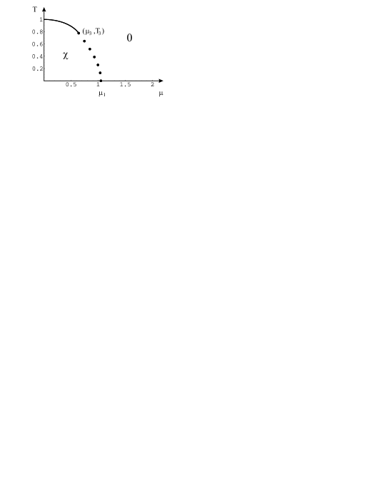
FIG. 1.: Phase diagram for $B/A\leq 0.418$ and $N_{c}=3$, as a function of the quark chemical potential $\mu$ and the temperature $T$. For this and all the following figures, continuous curves represent second-order lines while first-order lines are plotted with dots. Here, $\chi$ is the chiral phase and $\Delta$ is the diquark phase. First- and second-order lines join tangentially at the tricritical point $(\mu_{3},T_{3})$.

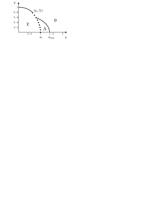
FIG. 2.: Phase diagram for the coupling ratio realized by single-gluon exchange, $B/A=0.75$. The transition from the chiral phase $\chi$ to the diquark phase $\Delta$ is first-order while that from the $\Delta$ to the trivial phase is second-order.

FIG. 3.: Phase diagram for a ratio $B/A=1.054$. The mixed broken symmetry phase $\chi\Delta$ emerges out of the chiral phase via a second-order transition at $\mu_{\rm mix}$, and undergoes a first-order transition towards the diquark phase at $\mu_{1}$.

FIG. 4.: Phase diagram for a ratio $B/A=1.1$. Compared to Fig. 3, the tricritical point $(\mu_{3},T_{3})$ no longer exists. The trivial, chiral, and diquark phases now meet at the new critical point $(\mu_{4},T_{4})$. We note in particular that the first and second-order lines bordering the chiral phase do not meet tangentially at $(\mu_{4},T_{4})$.

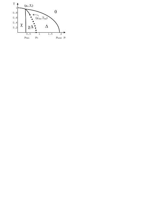
FIG. 5.: Phase diagram for a ratio $B/A=1.4$. Compared to Fig. 4, $(\mu_{4},T_{4})$ has become a tetracritical point, at the intersection of the four phases. There is also a new tricritical point $(\mu_{3\rm m},T_{3\rm m})$ where the first- and second-order line separating the $\chi\Delta$- and the $\Delta$-phases join tangentially.

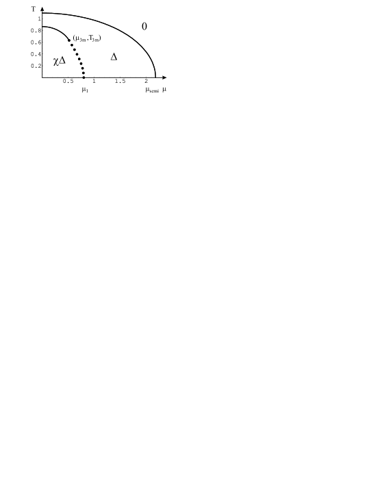
FIG. 6.: Phase diagram for a ratio $B/A=1.8$. This topology is characteristic of large ratios $B/A$, which favor diquark over chiral condensation. The $\Delta$-phase occupies a large part of the phase diagram, at the expense of the mixed broken symmetry phase. The chiral phase has completely vanished. We note that since Hermitian interactions realize ratios $B/A<1.5$, this last topology actually describes a case out of reach for our model.

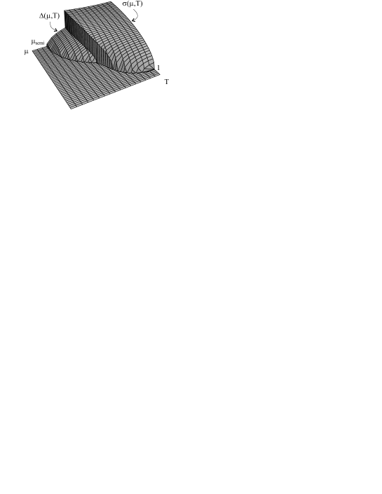
FIG. 7.: Order parameters for the coupling ratio of single-gluon exchange, $B/A=0.75$. The corresponding phase diagram is shown in Fig. 2. Chiral and diquark fields vanish continuously along the second-order lines.

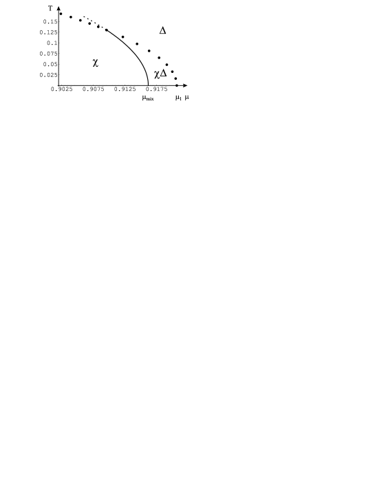
FIG. 8.: Expanded view of Fig. 3 near the wedge of mixed broken symmetry. We note that the second-order line between the $\chi$- to the $\chi\Delta$ phase does not meet tangentially with the first-order line between the $\chi\Delta$- and the $\Delta$-phases, as indicated by the short dashed line.

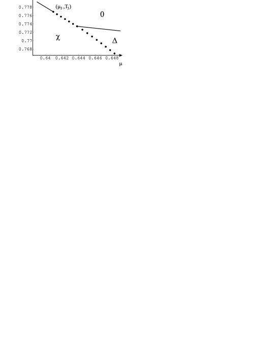
FIG. 9.: Expanded view of Fig. 3 near the tricritical point $(\mu_{3},T_{3})$, showing that there is a very short first-order segment between the chiral and trivial phases.

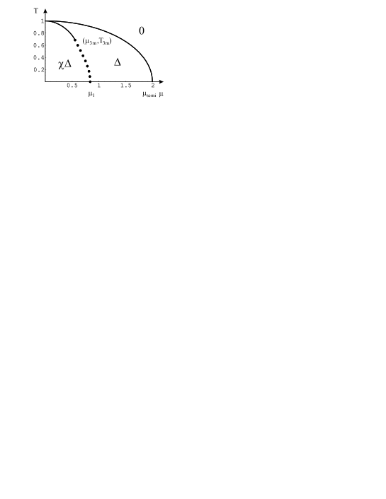
FIG. 10.: Phase diagram for the maximal ratio $B/A=1.5$ that can be realized by the random matrix interactions. With respect to Fig. 5, the thermodynamic competition favors the mixed broken symmetry phase at the expense of the chiral phase.

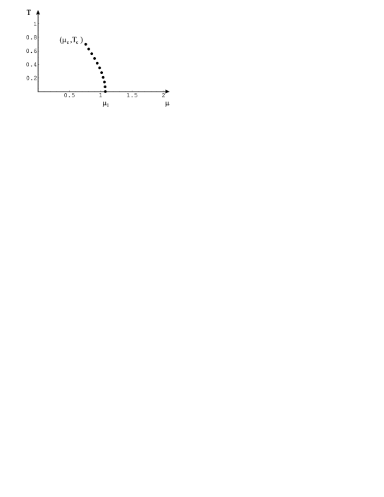
FIG. 11.: Phase diagram for a ratio $B/A=0.2$ and a small quark mass $m$.

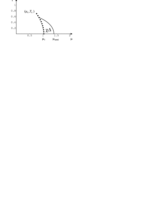
FIG. 12.: Phase diagram for the coupling ratio of single-gluon exchange, $B/A=0.75$, and a small quark mass $m\sim 10$ MeV. The first-order line ends at a critical point $(\mu_{c},T_{c})$.

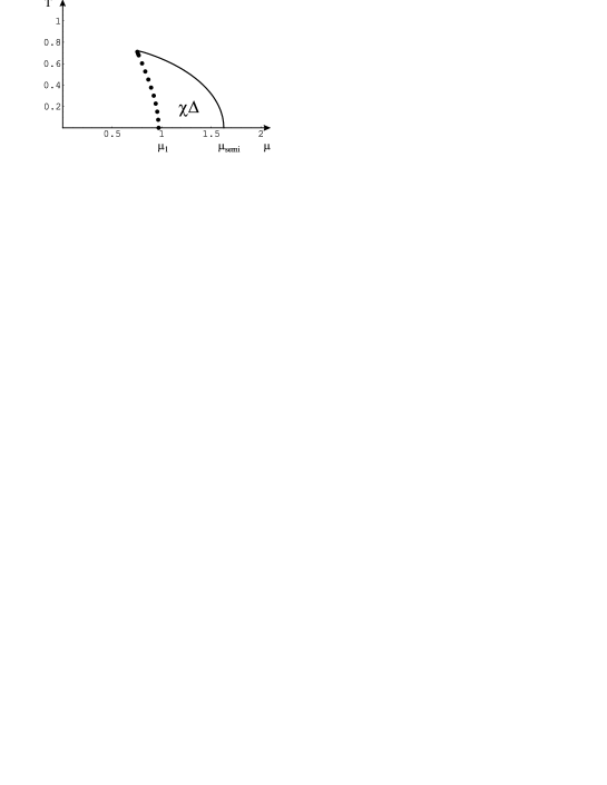
FIG. 13.: Phase diagram for $B/A=1.0$ and a small quark mass $m\sim 10$ MeV.

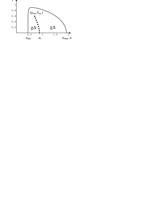
FIG. 14.: Phase diagram for $B/A=1.4$ and a small quark mass $m$. The first-order line ends at a critical point $(\mu_{\rm cm},T_{\rm cm})$.

Table 1. A few characteristic coupling ratios.
Ratio $B/A$		$N_{c}=2$			$N_{c}=3$			$N_{c}\to\infty$
Onset of diquark condensation					0.	418		0.	139	$N_{c}$
$\alpha_{1}(N_{c})$		1.	0		1.	050		0.	321	$N_{c}$
Disappearance of the tricritical point.					1.	061		0.	354	$N_{c}$
$\alpha_{2}(N_{c})$		1.	0		1.	163		0.	354	$N_{c}$
Maximum ratio $N_{c}/2$		1.	0		1.	5		0.	5	$N_{c}$
Single-gluon exchange		1.	0		0.	75		0.	5

REFERENCES

- [1] B. Barrois, Nucl. Phys. B129, 390 (1977);
- [2] D. Bailin and A. Love, Phys. Rept. 107, 325 (1984).
- [3] M. Alford, K. Rajagopal, and F. Wilczek, Phys. Lett. B 422, 247 (1998).
- [4] R. Rapp, T. Schäfer, E. V. Shuryak, and M. Velkovsky, Phys. Rev. Lett. 81, 53 (1998); hep-ph/9904353.
- [5] G. W. Carter and D. Diakonov, Phys. Rev. D 60, 016004 (1999).
- [6] J. Berges and K. Rajagopal, Nucl. Phys. B538, 215 (1999).
- [7] T. M. Schwarz, S. P. Klevansky, and G. Papp, Phys. Rev. C 60, 055205 (1999).
- [8] For studies of diquark condensation at low densities, see also S. Ying, Phys. Lett B 285, 341 (1992); Ann. Phys. (N. Y.) 250, 69 (1996); S. Pépin, M. C. Birse, J. A. McGovern, and N. R. Walet, hep-ph/9912475.
- [9] B. Vanderheyden and A. D. Jackson, Phys. Rev. D 61, 076004 (2000).
- [10] See the procceedings of QCD at finite baryon densities, Bielfeld, April 1998, F. Karsh and M. P. Lombardo (Eds.), Nucl. Phys. A642 (1998).
- [11] M. A. Stephanov, Phys. Rev. Lett. 76, 4471 (1996); Nucl. Phys. Proc. Suppl. 53, 469 (1997).
- [12] J. Kogut, H. Matsuoka, M. Stone, H.W. Wyld, S. Shenker, J. Shigemitsu, and D. K. Sinclair, Nucl. Phys. B225 [FS9], 93 (1983).
- [13] I. M. Barbour, N. Behlil, E. Dagotta, F. Karsch, A. Moreao, M. Stone, and H. W. Wyld, Nucl. Phys. B275 [FS17] 296, (1986).
- [14] J. B. Kogut, M. P. Lombardo, and D. K. Sinclair, Phys. Rev D 51, 1282 (1995).
- [15] I. M. Barbour, S. E. Morrison, E. G. Klepfish, J. B. Kogut, and M. P. Lombardo, Phys. Rev. D 56, 7063 (1997).
- [16] E. V. Shuryak and J. J. M. Verbaarschot, Nucl. Phys. A560, 306 (1993).
- [17] J. J. M. Verbaarschot, Phys. Rev. Lett. 72 2531 (1994); Phys. Lett. B 329, 351 (1994).
- [18] For a review, see J. J. M. Verbaarschot, hep-ph/9902394.
- [19] T. Banks and A. Casher, Nucl. Phys. B169, 103 (1980).
- [20] M.A. Halasz, A.D. Jackson, R.E. Shrock, M.A. Stephanov, J.J.M. Verbaarschot, Phys.Rev. D 58, 096007 (1998).
- [21] A. D. Jackson and J. J. M. Verbaarschot, Phys. Rev. D53, 7223 (1996).
- [22] I. D. Lawrie and S. Larbach, in Phase Transitions and Critical Phenomena, Edited by C. Domb and J. L. Lebowitz (Academic Press, London, 1984), vol. 9, p. 1.
- [23] D. Diakonov and V. Petrov, in Quark Cluster Dynamics, Lecture Notes in Physics, edited by K. Goeke, P. Kroll, and H. Petry (Springer-Verlag, Berlin, 1992) p. 288.
- [24] A. Smilga and J. J. M. Verbaarschot, Phys. Rev. D 51, 829 (1995).
- [25] J. B. Kogut, M. A. Stephanov, and D. Toublan, Phys. Lett. B 464, 183 (1999).
- [26] D. Diakonov, H. Forkel, and M. Lutz, Phys. Lett. B373, 147 (1996).
- [27] E. Dagotta, F. Karsh, and A. Moreo, Phys. Lett. B 169, 421 (1986).
- [28] G. ’t Hooft, Nucl. Phys. B72, 461 (1972).