BOTTOM PRODUCTION

Abstract

We review the prospects for bottom production physics at the LHC.

1 INTRODUCTION

In the context of the LHC experiments, the physics of bottom flavoured hadrons enters in different contexts. It can be used for QCD tests, it affects the possibilities of $B$ decays studies, and it is an important source of background for several processes of interest.

The physics of $b$ production at hadron colliders has a rather long story, dating back to its first observation in the UA1 experiment. Subsequently, $b$ production has been studied at the Tevatron. Besides the transverse momentum spectrum of a single $b$, it has also become possible, in recent time, to study correlations in the production characteristics of the $b$ and the $\overline{b}$.

At the LHC new opportunities will be offered by the high statistics and the high energy reach. One expects to be able to study the transverse momentum spectrum at higher transverse momenta, and also to exploit the large statistics to perform more accurate studies of correlations.

This chapter is organized as follows.

Section 2 is mostly theoretical. Its goal is to provide benchmark cross sections and distributions for the LHC, including rates relevant for the trigger requirements of the experiments. Furthermore, a discussion of the present status of $b$ production phenomenology at hadron colliders is given. In this context, one cannot forget that the theoretical status is a mixed success. On one side, the shape of distributions and correlations are reasonably well explained by perturbative QCD. On the other side, however, the observed cross sections at the Tevatron are larger than QCD predictions. It is hoped that further studies may help to understand the nature of the discrepancy. As of now, we see two possible explanations: either the absolute normalization of the cross section is not correctly predicted due to the presence of large higher order terms, or the shape of the distributions is distorted by some perturbative or non-perturbative effects (like, for example, fragmentation effects). With the wide $p_{\scriptscriptstyle T}$ range covered by the LHC experiments, and perhaps also with the possibility of performing more accurate studies of correlations, these two possibilities may be distinguished. The problem of fragmentation effects has been studied in this workshop also from the point of view of hadronization models in Monte Carlo programs, in Section 3. This study deals with the hadronization model in the HERWIG Monte Carlo program. Its aim was to understand whether, in simple realistic models of hadronization, the usual assumption of QCD factorization is really at work. In general, the problem of studying how realistic is the heavy flavour production mechanism implemented in shower Monte Carlo’s is quite important, and probably will require a considerable effort. Along this line, in Section 4, a problem in the heavy flavour production mechanisms implemented in Pythia is examined.

Further self-contained theoretical topics are dealt with in Sections 5 and 6. Section 5 deals with the charge asymmetry in $b$ production in $pp$ collisions. In this context, QCD is not of great help, since in perturbative QCD charge asymmetries turn out to be extremely small. Instead, studies are made within specific hadronization models, that are parametrized in such a way that they fit charm asymmetry data. This topic, besides being interesting in its own, since it deals with a phenomenon which is dominated by non-perturbative physics, has also an impact on $CP$ violation studies in $B$ decays.

In Section 6 quarkonium production is discussed. This subject has been intensively studied in recent years, following an initial CDF observation of a $J/\Psi$ production rate much higher than theoretical predictions. This has triggered, from the theoretical side, the understanding that the fragmentation process is the dominant mechanism in quarkonium production. Besides this, a novel branch of applications of perturbative QCD, the NRQCD approach, has emerged, that may be useful to explain the production process.

In Section 7, the prospects for $b$ detection are discussed. It is shown that there is a complementarity between ATLAS/CMS and the LHCb experiment, with a certain region of overlap. In particular, the LHCb experiment can detect very low momentum heavy quarks, while the other experiments can reach the very high transverse momentum region. Some results on correlations measurements are also given, exploring the possibility of looking at one $b$ decaying into a $J/\Psi$, and the other decaying semileptonically. Double heavy flavour production, charge asymmetry, polarization effects, and doubly-heavy meson production are also discussed.

In Section 8 the tuning of the multiple interaction parameters in Pythia is illustrated. The correct treatment of multiple interactions is important to model the multiplicity observables in both minimum-bias and heavy flavour events.

2 BENCHMARK CROSS SECTIONS

2.1 Total cross sections

It is assumed that heavy flavour production in hadronic collisions can be described in the usual improved parton model approach, where light partons in the incoming hadrons collide and produce a heavy quark-antiquark pair via elementary strong interaction vertices, like, for example, in the diagram of fig. 1.

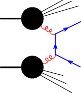
Figure 1: Typical diagram for heavy flavour production

This description is appropriate for all hard processes in hadronic collisions, and thus, in the case of heavy flavours, is applicable as long as the mass of the heavy flavour can be considered sufficiently large. The perturbative QCD cross section for heavy flavour production has been computed to next-to-leading order accuracy (i.e. ${\cal O}(\alpha_{\scriptscriptstyle\rm S}^{3})$) a long time ago [1] [2] [3] [4] [5] [6] [7] [8] [9] [10] [11], and a large amount of experimental and theoretical work has been done in this field. A relatively recent account of the status of this field can be found in ref. [12]. It can be said that qualitatively the QCD description of heavy flavour production seems to be adequate also for charm production, while quantitatively large uncertainties are present in the calculation of the charm and bottom cross section. Only for a quark as heavy as the top quark the perturbative calculation seems (up to now) to predict the cross section with a good accuracy.

Large uncertainties are also found in the calculation of the bottom production cross section at the LHC. The largest uncertainty is due to unknown higher order effects, and it is traditionally quantified by estimating the scale dependence of the cross section when the renormalization and factorization scales are varied by a factor of 2 above and below their central value, which is usually taken equal to the heavy quark mass. Since this uncertainty is due to a limitation in our current theoretical knowledge, it is hard to overcome. Other sources of uncertainty are related to theoretical and experimental errors in the parameters that enter the perturbative calculation: the value of the strong coupling constant, the heavy quark mass, and the parton density functions.

We present here a benchmark study of $b$ total cross sections at the LHC, using the FMNR package for heavy flavour cross sections [5] [8] (the code for this package is available upon request to the authors). In the study we consider

• The dependence of the total cross section on the choice of the factorization and renormalization scales. We will use the values $\mu=m_{b},2m_{b},m_{b}/2$.

• The dependence on the parton density parametrization. We will use the sets MRST [13], MRST$(g{\scriptstyle\uparrow})$, MRST$(g{\scriptstyle\downarrow})$, MRST$(\alpha_{\scriptscriptstyle\rm S}{\scriptstyle\downarrow})$ and MRST$(\alpha_{\scriptscriptstyle\rm S}{\scriptstyle\uparrow})$. The first set is used as reference set. MRST$(g{\scriptstyle\uparrow})$ and MRST$(g{\scriptstyle\downarrow})$ have extreme gluon densities, MRST$(\alpha_{\scriptscriptstyle\rm S}{\scriptstyle\downarrow})$-MRST$(\alpha_{\scriptscriptstyle\rm S}{\scriptstyle\uparrow})$ have extreme values of the strong coupling constant: $\Lambda_{5}=220\;$MeV for MRST, 164 MeV for MRST$(\alpha_{\scriptscriptstyle\rm S}{\scriptstyle\downarrow})$, 280 MeV for MRST$(\alpha_{\scriptscriptstyle\rm S}{\scriptstyle\uparrow})$. Cross section values obtained with the CTEQ4 [14] set are very similar to the MRST set. We have preferred to use the MRST sets because they gave us the possibility to perform a study of sensitivity to $\Lambda$ and to variations in the gluon density.

• The dependence on the $b$ quark mass: $m_{b}=4.75\pm 0.25\;$GeV.

Factorization and renormalization scale dependence of the total cross section at $\sqrt{S}=14\;$TeV is reported in table 1, where we have used the MRST parton densities, with $\Lambda_{5}=220\;$MeV, and we have fixed the $b$ mass at the value $m_{b}=4.75\;$GeV.

Table 1: Dependence of the $b$ cross section on scale choices.

$\mu_{\rm F}/m_{b}$	$\mu_{\rm R}/m_{b}$	Total ($\mu b$)	Born ($\mu b$)
0.50	1.00	0.2779 $10^{3}$	0.6465 $10^{2}$
1.00	1.00	0.4960 $10^{3}$	0.1796 $10^{3}$
2.00	1.00	0.6453 $10^{3}$	0.3253 $10^{3}$
0.50	0.50	0.5126 $10^{3}$	0.1078 $10^{3}$
1.00	0.50	0.8289 $10^{3}$	0.2995 $10^{3}$
2.00	0.50	0.9538 $10^{3}$	0.5426 $10^{3}$
0.50	2.00	0.1758 $10^{3}$	0.4355 $10^{2}$
1.00	2.00	0.3353 $10^{3}$	0.1209 $10^{3}$
2.00	2.00	0.4669 $10^{3}$	0.2191 $10^{3}$

Notice that:

• If we keep $\mu_{\rm F}=\mu_{\rm R}$, the full cross section variation is small (467 to 512 $\mu b$).

• The largest cross section corresponds to large $\mu_{\rm F}$ and small $\mu_{\rm R}$

• The smallest cross section corresponds to small $\mu_{\rm F}$ and large $\mu_{\rm R}$

This is understood since, at small $x$, the gluon density $g(x)$ grows with the scale, and $\alpha_{\scriptscriptstyle\rm S}$ decreases with the scale.

The dependence on the choice of parton density parametrization is shown in table 2.

Table 2: Parton density dependence of total cross sections (in $\mu b$).

	central	lowest	highest
MRST	0.4960 $10^{3}$	0.1758 $10^{3}$	0.9538 $10^{3}$
MRST$(g{\scriptstyle\uparrow})$	0.4866 $10^{3}$	0.1727 $10^{3}$	0.9337 $10^{3}$
MRST$(g{\scriptstyle\downarrow})$	0.4992 $10^{3}$	0.1751 $10^{3}$	0.9610 $10^{3}$
MRST$(\alpha_{\scriptscriptstyle\rm S}{\scriptstyle\downarrow})$	0.4487 $10^{3}$	0.1799 $10^{3}$	0.7878 $10^{3}$
MRST$(\alpha_{\scriptscriptstyle\rm S}{\scriptstyle\uparrow})$	0.6001 $10^{3}$	0.1894 $10^{3}$	0.1267 $10^{4}$

As one can see, the sensitivity to the variation of the gluon density is small. Apparently, the constraints from HERA data are strong enough in the $x$ region where most of the $b$ production takes place. The dependence upon the strong coupling constant is instead larger, and can increase the upper limit of the cross section by about 40%. The last two sets have $\Lambda_{5}=164$ and 288 MeV respectively, corresponding to $\alpha_{\scriptscriptstyle\rm S}(M_{Z})=0.1125$ and 0.1225, which is a reasonably large range.

Mass uncertainties are quite important, especially if $m_{b}$ is allowed to take very small values. This can be seen from table 3.

Table 3: Mass dependence of total cross sections (in $\mu b$).

$m_{b}$ (GeV)	central	lowest	highest
4	0.7957 $10^{3}$	0.2336 $10^{3}$	0.1706 $10^{4}$
4.5	0.5789 $10^{3}$	0.1945 $10^{3}$	0.1138 $10^{4}$
5	0.4313 $10^{3}$	0.1609 $10^{3}$	0.8087 $10^{3}$

We see that lowering the $b$ mass from 4.5 down to 4 GeV raises the upper limit of the cross section by about 50%. It is however unlikely that such small values are viable. A rough view of the status of the bottom mass determination is given in fig. 2,

Figure 2: Different determinations of the $b$ quark pole mass.

which we obtained by taking the various determinations of the ${\overline{\rm MS}}$ bottom mass from the Particle Data Book, and rescale them by a factor of (1+0.09+0.06), to account for the two-loop correction needed to translate the ${\overline{\rm MS}}$ mass into the pole mass. As one can see, not all determinations are consistent among each other. A critical review of all determinations is beyond the scope of this workshop. We should however point out that recent progress has been made in the bottom mass determination. The reader can find a summary of these issues and further references in ref. [15]. It is argued there that the bottom mass is determined with higher precision in processes where it is probed at short distances, like in the $\Upsilon$ mass, or via sum rules applied to the bottom vector current spectral function in $e^{+}e^{-}$ annihilation. The mass extracted in this way can be reliably related to the so called ${\overline{\rm MS}}$ mass. The relation of the ${\overline{\rm MS}}$ mass to the pole mass is instead not so precise, because the perturbative expansion that relates the two quantities is not convergent. In ref. [15] a preferred value of $\bar{m}_{b}(m_{b})=4.23\pm 0.08$ is given, where $\bar{m}_{b}(m_{b})$ is the $\overline{\rm MS}$  bottom mass at the scale of the bottom mass itself. The corresponding pole mass, obtained using the newly computed 3-loop relation between the ${\overline{\rm MS}}$ and pole mass [16] [17], is $4.98\pm 0.09$ GeV. If one wanted to account for the uncertainties due to the lack of convergence of the perturbative expansion, the range obtained in this way should be enlarged by some amount, of the order of 100 MeV. The question arises whether it would be possible to eliminate this uncertainty by expressing the hadroproduction cross section in terms of the $\overline{\rm MS}$  mass. In our view, the answer is most likely no, since the bottom hadroproduction cross section does not have the same inclusive character as the sum rules applied to the $e^{+}e^{-}$ bottom spectral function.

In the present work we thus used the traditional range $4.5$ GeV $<m_{b}<5$ GeV for the bottom pole mass in the hadroproduction process, keeping in mind that recent determinations seem to favour the upper region of this range. The sensitivity of the cross section to the bottom mass in this range is at most of $\pm 10$%, and it becomes much smaller if transverse momentum cuts are applied. Thus, as far as the LHC is concerned, this uncertainty is not very important.

The largest uncertainy in the cross section comes from the scale uncertainty, which is a (rather arbitrary) method to assess the possible impact of unknown higher order corrections. In the following we report a brief discussion of the origin of these large corrections. Radiative corrections for the total cross section are usually parametrized as follows. The total cross sections $\sigma_{ij}$ for the various parton subprocesses (${\overline{q}}q,qg,gg$) have a perturbative expansions given by

$$\sigma_{ij}=\frac{\alpha_{\scriptscriptstyle\rm S}^{2}(\mu)}{m^{2}}\left[f_{ij}^{(0)}(\rho)+4\pi\alpha_{\scriptscriptstyle\rm S}\left(f_{ij}^{(1)}(\rho)+\bar{f}^{(1)}(\rho)\log\frac{\mu^{2}}{m^{2}}\right)\right],$$ (1)

where $\rho=4m_{b}^{2}/\hat{s}$ and $\hat{s}$ is the squared partonic center-of-mass energy. The functions $f_{ij}^{(0,1)}$ for the ${\overline{q}}q$ and $gg$ subprocesses are displayed in fig. 3.

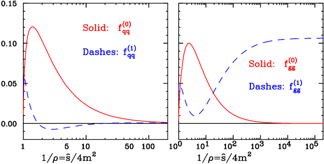
Figure 3: Partonic cross section for the $q\bar{q}$ and $gg$ subprocesses.

Notice the behaviour near threshold

$$f_{q\overline{q}}^{(1)}\rightarrow\frac{f^{(0)}_{q\bar{q}}(\rho)}{8\pi^{2}}\Bigg{[}-\frac{\pi^{2}}{6\beta}+\frac{16}{3}\ln^{2}\big{(}8\beta^{2}\big{)}-\frac{82}{3}\ln(8\beta^{2})\Bigg{]}$$

$$f_{gg}^{(1)}\rightarrow\frac{f_{gg}^{(0)}(\rho)}{8\pi^{2}}\Bigg{[}\frac{11\pi^{2}}{42\beta}+12\ln^{2}\big{(}8\beta^{2}\big{)}-\frac{366}{7}\ln(8\beta^{2})\Bigg{]}$$

due to Coulomb $1/\beta$ singularities and to Sudakov double logarithms. Near threshold, these terms may require special treatement, such as resummation to all orders. Notice also the constant asymptotic behaviour of $f^{(1)}_{gg}$, which may cause problems far above threshold.

Plotting the cross section as a function of the partonic energy $\hat{s}$ may help to understand the origin of large corrections.

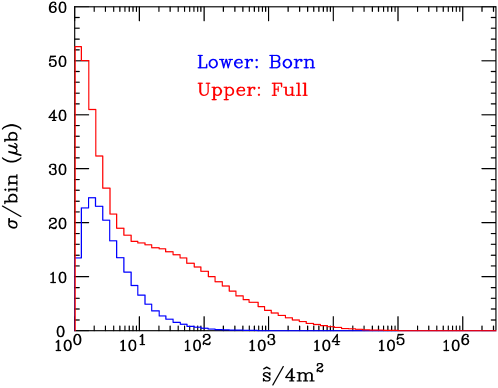
Figure 4: Partonic cross section as a function of $\hat{s}/4m^{2}$

.

We find that radiative corrections are large near the production threshold. This problem becomes more and more severe as we approach the production threshold. Thus, it is more important for production of $b$ at fixed target energies, or for production of $t\bar{t}$ pairs at colliders. Techniques to resum these large corrections to all orders of perturbation theory, at the NLO level are available [18], but it is found that little improvement is achieved for the bottom cross section at collider energies. Large corrections are also found far above threshold. This effect is bound to become more and more pronounced in the high energy limit. In order to reduce the scale uncertainties coming from these corrections, one should resum them at the next-to-leading order level. This problem has been discussed in the literature, so far, only at the leading logarithmic level [19] [20] [21] [22]. At the time of the completion of this workshop, no further progress has been achieved in this field.

In fig. 5 we present a study of the scale dependence of the total cross section as a function of $\rho$.

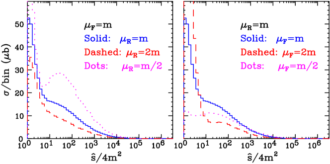
Figure 5: Scale dependence of the total cross section.

We find a large scale dependence near threshold, due to both renormalization and factorization scale variation, and a large scale dependence far from threshold. Here, the renormalization scale dependence plays a dominant role. Renormalization scale variations are mainly due to the large variation of the coupling constant in the ${\cal O}(\alpha_{\scriptscriptstyle\rm S}^{3})$ terms. Where radiative corrections are small, a reasonable scale compensation takes place. Thus, both the threshold and the high energy regions, where corrections are large, are strongly affected. Factorization scale variation has a strong impact on threshold corrections, while in the high energy region we observe some compensation. In fact, the cross section near threshold increases with $\mu_{\rm F}$ near threshold, while above threshold the $\mu_{\rm F}=m$ value is above both the $\mu_{\rm F}=m/2$ and the $\mu_{\rm F}=2m$ curves, indicating the presence of some sort of compensation. As of now, it appears therefore that a better understanding of the high energy region will not strongly reduce the scale uncertainty, although it might, of course, improve our confidence in the error band we quote.

The study given here deals with total cross sections. It should be repeated with appropriate rapidity cuts, since this may reduce large effects due to the high energy limit. In general, we may expect that the cross section with rapidity and transverse momentum cuts may have smaller error bars than the total. It is particularly interesting to investigate directly cross sections for muons originating from $B$ decays, since muons are often used as trigger objects for $B$ physics. We have performed this study using a simple implementation of the $B$ semileptonic decay in the FMNR program, that will be described in more details in the following subsections. The results are shown in table 4.

Table 4: Cross sections (in $\mu b$) for $b\mbox{$\rightarrow$}\mu+X$ production, with a muon, or both, satisfying appropriate cuts. Only muons coming directly from $B$ decays are included here. The calculation was performed using the CTQ4M parton densities. The upper number are the maximum, and the lower number the minimum of the values obtained by varying the scales in the usual way. The corresponding total cross sectios are 165 to 864 $\mu{\rm b}$ The $B\mbox{$\rightarrow$}\mu$ branching fraction was taken equal to 10.5%. Different values for the $\epsilon$ parameter of the Peterson fragmentation function are assumed. The last two column show the impact of a rather large intrinsic transverse momentum of the incoming partons.

$\epsilon$	0	0.002	0.006	0.002	0.006
$\langle k_{T}\rangle$ (GeV)	0	0	0	4	4
A: $b\bar{b}\mbox{$\rightarrow$}\mu(|\eta|<2.4,\;p_{T}\geq 6)$	$3.3\atop 1.06$	$2.41\atop 0.81$	$2.12\atop 0.72$	$3.4\atop 1.06$	$2.91\atop 0.94$
B: $b\bar{b}\mbox{$\rightarrow$}\mu(p_{T}>6)\;\mu(p_{T}>3)$	$0.76\atop 0.304$	$0.52\atop 0.219$	$0.45\atop 0.19$	$0.67\atop 0.252$	$0.54\atop 0.214$
C: $b\bar{b}\mbox{$\rightarrow$}\mu(p_{T}>6)\;e(p_{T}>2)$	$1.18\atop 0.43$	$0.83\atop 0.32$	$0.71\atop 0.277$	$1.1\atop 0.38$	$0.92\atop 0.33$
D: $b\bar{b}\mbox{$\rightarrow$}\mu(p_{T}>7,\;|\eta|<2.4)$	$2.26\atop 0.78$	$1.62\atop 0.58$	$1.41\atop 0.5$	$2.23\atop 0.73$	$1.9\atop 0.63$
E: $b\bar{b}\mbox{$\rightarrow$}\mu(p_{T}>7,\;|\eta|<2.4)$
E: $b\bar{b}\mbox{$\rightarrow$}$ $\mu(p_{T}>4.5,\;\;0<|\eta|<1.5)$	$0.0304\atop 0.0146$	$0.0203\atop 0.0102$	$0.0174\atop 0.0087$	$0.0232\atop 0.0105$	$0.0188\atop 0.009$
F: $b\bar{b}\mbox{$\rightarrow$}\mu(p_{T}>7,\;|\eta|<2.4)$
F: $b\bar{b}\mbox{$\rightarrow$}$ $\mu(p_{T}>3.6,\;1.5<|\eta|<2)$	$0.0101\atop 0.0045$	$0.0075\atop 0.0032$	$0.0068\atop 0.0026$	$0.0096\atop 0.0035$	$0.0076\atop 0.00281$
G: $b\bar{b}\mbox{$\rightarrow$}\mu(p_{T}>7,\;|\eta|<2.4)$
G: $b\bar{b}\mbox{$\rightarrow$}$ $\mu(p_{T}>2.6,\;2<|\eta|<2.4)$	$0.0105\atop 0.0038$	$0.0073\atop 0.00263$	$0.0053\atop 0.00219$	$0.0082\atop 0.00251$	$0.0062\atop 0.0024$
H: $b\bar{b}\mbox{$\rightarrow$}\mu(p_{T}>1,\;2<|\eta|<6)$	$19.3\atop 5.4$	$18.8\atop 5.3$	$18.6\atop 5.2$	$19.1\atop 5.4$	$18.9\atop 5.3$
I: $b\bar{b}\mbox{$\rightarrow$}\mu(p_{T}>2,\;2<|\eta|<6)$	$10.2\atop 2.94$	$9.1\atop 2.65$	$8.6\atop 2.51$	$10.6\atop 3.11$	$10.\atop 2.96$

The same results are also reported in fig. 6, since several features become more apparent there.

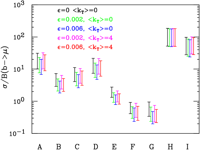
Figure 6: Cross sections as in table 4. The four bars in each group correspond to different choices of $\epsilon$ and $\langle k_{T}\rangle$, in the order reported in the figure.

First of all, we point out that, as expected, there is a considerable reduction in the scale dependence in these muon rates. This is mostly due to the presence of cuts in the transverse momentum of the muon, that increases the total transverse energy that characterizes the cross section. Thus, while the ratio of the upper to the lower limit of the cross section is above a factor of 5 in the total rate, it is between a factor of 2 and 4 in the muon rates. The smallest values are achieved for the highest momentum cuts. A non perturbative fragmentation function of the Peterson form was also included in the calculation, with $\epsilon$ parameter taking the values $0$ (i.e., no fragmentation), $0.002$ and $0.006$. More details on its implementation are given in the following subsections. Observe that for softer fragmentation functions (i.e. larger $\epsilon$ parameter) the uncertainty is reduced, since they imply higher quark momenta. The reduction in the scale uncertainty is obtained at the price of introducing a sensitivity to the fragmentation function parameter. We considered as realistic values of $\epsilon$ between 0.002 and 0.006. The corresponding variation of the cross section is not large. The impact of an intrinsic transverse momentum of the incoming partons (see the following subsections) is also studied. We have chosen the unrealistically large value $\langle k_{T}\rangle=4$ GeV just to show that its effect is in all cases not a dramatic one.

2.2 Transverse momentum spectrum

2.2.1 Benchmark single-inclusive distributions

The fixed-order, NLO result for single-inclusive $b$ production has several limitations in different regions of the phase space. In particular, one should be aware of the high-energy limit problem when $p_{T}$ is small compared to the incoming energy, of the logarithms of $m_{b}/p_{T}$ for high transverse momenta, and of further problems when approaching the threshold region. All these issues will be discussed in some detail in the next Sections. However, the fixed-order calculation at NLO provides a useful starting point for estimating the differential cross section. At this time, it is probably not useful to perform a cross section study with different sets of parton densities, and for different values of the $b$ mass. We limit ourselves to the MRST set, and we only study the scale dependence of the cross section. We do not include, at this stage, fragmentation effects, which, as shown in the following Sections, can be easily accounted for. In tables 5-8 we collect the results of this study.

Table 5: Differential cross section $d\sigma/dp_{T}^{2}dy$ for single inclusive $b$ production at the LHC, for $p_{T}$ from 1 to 80 GeV and $y$ from 0 to 4. The table was computed with the $MRST$ parton density set, for $m_{b}=4.75\;$GeV. The central value was obtained with the factorization and renormalization scale set to $\sqrt{p_{T}^{2}+m^{2}}$. The upper and lower values give the maximal variation when varying the scales independently by a factor of 2 above and below the central value. Cross sections are in $\mu b$; each element in a row should be multiplied by the common scale factor in the left column.

$y$	0	1	1.5	2	2.5	3	3.5	4
$p_{T}=1$	$7.7$	$7.6$	$7.5$	$7.3$	$7$	$6.6$	$6.1$	$5.4$
$10^{-1}\times$	$23.9$	$23.4$	$22.7$	$21.8$	$20.6$	$19.1$	$17.2$	$14.6$
	$41.3$	$40.5$	$39.5$	$38.2$	$36.4$	$34.1$	$31$	$26.1$
$p_{T}=2$	$6.7$	$6.6$	$6.5$	$6.3$	$6$	$5.7$	$5.2$	$4.56$
$10^{-1}\times$	$19.2$	$18.8$	$18.2$	$17.4$	$16.4$	$15.1$	$13.5$	$11.5$
	$30.3$	$29.7$	$29$	$28$	$26.7$	$24.9$	$22.6$	$19.2$
$p_{T}=3$	$5.4$	$5.3$	$5.2$	$5$	$4.76$	$4.43$	$4.01$	$3.48$
$10^{-1}\times$	$14$	$13.6$	$13.2$	$12.6$	$11.8$	$10.8$	$9.5$	$8$
	$21.8$	$21.3$	$20.7$	$19.9$	$18.8$	$17.4$	$15.6$	$13.2$
$p_{T}=4$	$4.04$	$3.96$	$3.85$	$3.7$	$3.48$	$3.21$	$2.87$	$2.45$
$10^{-1}\times$	$9.9$	$9.6$	$9.3$	$8.8$	$8.2$	$7.4$	$6.5$	$5.4$
	$15.9$	$15.5$	$15$	$14.2$	$13.3$	$12.1$	$10.6$	$8.9$
$p_{T}=5$	$2.91$	$2.84$	$2.75$	$2.62$	$2.45$	$2.24$	$1.97$	$1.64$
$10^{-1}\times$	$6.6$	$6.4$	$6.2$	$5.8$	$5.3$	$4.79$	$4.13$	$3.37$
	$11.1$	$10.7$	$10.3$	$9.7$	$9$	$8$	$6.9$	$5.7$
$p_{T}=7$	$14$	$13.6$	$13.1$	$12.3$	$11.3$	$10.1$	$8.6$	$6.9$
$10^{-2}\times$	$29.4$	$28.2$	$26.9$	$25$	$22.7$	$19.8$	$16.6$	$13$
	$51$	$48.5$	$46$	$42.7$	$38.5$	$33.5$	$27.9$	$21.7$
$p_{T}=10$	$4.72$	$4.54$	$4.31$	$3.99$	$3.58$	$3.09$	$2.52$	$1.9$
$10^{-2}\times$	$9.1$	$8.7$	$8.2$	$7.5$	$6.6$	$5.6$	$4.49$	$3.32$
	$15.6$	$14.8$	$13.9$	$12.6$	$11.1$	$9.3$	$7.4$	$5.4$
$p_{T}=15$	$10.3$	$9.8$	$9.1$	$8.2$	$7.1$	$5.9$	$4.49$	$3.11$
$10^{-3}\times$	$17.8$	$16.8$	$15.6$	$14$	$12$	$9.7$	$7.3$	$4.91$
	$29.3$	$27.5$	$25.4$	$22.6$	$19.2$	$15.4$	$11.4$	$7.6$
$p_{T}=20$	$2.99$	$2.81$	$2.6$	$2.3$	$1.94$	$1.53$	$1.1$	$0.7$
$10^{-3}\times$	$4.86$	$4.55$	$4.16$	$3.65$	$3.04$	$2.36$	$1.67$	$1.04$
	$7.7$	$7.1$	$6.5$	$5.7$	$4.69$	$3.61$	$2.52$	$1.55$
$p_{T}=30$	$4.53$	$4.2$	$3.79$	$3.25$	$2.61$	$1.91$	$1.25$	$0.68$
$10^{-4}\times$	$6.8$	$6.3$	$5.6$	$4.77$	$3.78$	$2.74$	$1.75$	$0.93$
	$10.1$	$9.3$	$8.3$	$7$	$5.5$	$3.94$	$2.49$	$1.3$
$p_{T}=40$	$10.9$	$10$	$8.8$	$7.4$	$5.7$	$3.9$	$2.31$	$1.08$
$10^{-5}\times$	$15.5$	$14.1$	$12.5$	$10.3$	$7.8$	$5.3$	$3.1$	$1.41$
	$22.3$	$20.2$	$17.8$	$14.6$	$11$	$7.4$	$4.23$	$1.92$
$p_{T}=50$	$3.47$	$3.13$	$2.72$	$2.21$	$1.63$	$1.06$	$0.57$	$0.218$
$10^{-5}\times$	$4.77$	$4.28$	$3.71$	$2.99$	$2.18$	$1.4$	$0.74$	$0.287$
	$6.7$	$6$	$5.2$	$4.12$	$2.98$	$1.89$	$1.01$	$0.395$
$p_{T}=60$	$13.2$	$11.8$	$10.1$	$8$	$5.7$	$3.48$	$1.66$	$0.53$
$10^{-6}\times$	$17.8$	$15.8$	$13.5$	$10.6$	$7.5$	$4.52$	$2.18$	$0.71$
	$24.3$	$21.5$	$18.3$	$14.3$	$10$	$6.1$	$2.97$	$0.98$
$p_{T}=80$	$2.77$	$2.42$	$2.01$	$1.5$	$0.98$	$0.53$	$0.207$	$0.0449$
$10^{-6}\times$	$3.59$	$3.12$	$2.59$	$1.95$	$1.28$	$0.69$	$0.273$	$0.06$
	$4.76$	$4.14$	$3.45$	$2.6$	$1.72$	$0.94$	$0.376$	$0.083$

Table 6: As in table 5, for $y$ from 4.5 to 6.5.

$y$	4.5	5	5.5	6	6.5
$p_{T}=1$	$4.51$	$3.46$	$2.36$	$1.36$	$0.59$
$10^{-1}\times$	$11.6$	$8.4$	$5.3$	$2.87$	$1.15$
	$20$	$14.2$	$8.5$	$4.47$	$1.8$
$p_{T}=2$	$3.74$	$2.82$	$1.88$	$1.04$	$0.431$
$10^{-1}\times$	$9$	$6.4$	$4.04$	$2.1$	$0.8$
	$14.6$	$10.2$	$6.3$	$3.2$	$1.23$
$p_{T}=3$	$2.8$	$2.06$	$1.32$	$0.69$	$0.261$
$10^{-1}\times$	$6.2$	$4.35$	$2.65$	$1.31$	$0.458$
	$10.1$	$6.8$	$4.07$	$1.97$	$0.7$
$p_{T}=4$	$1.93$	$1.37$	$0.84$	$0.415$	$0.137$
$10^{-1}\times$	$4.08$	$2.78$	$1.62$	$0.75$	$0.231$
	$6.7$	$4.44$	$2.53$	$1.15$	$0.35$
$p_{T}=5$	$1.27$	$0.87$	$0.51$	$0.233$	$0.065$
$10^{-1}\times$	$2.52$	$1.67$	$0.93$	$0.404$	$0.105$
	$4.19$	$2.71$	$1.5$	$0.63$	$0.16$
$p_{T}=7$	$5.1$	$3.24$	$1.71$	$0.65$	$0.12$
$10^{-2}\times$	$9.3$	$5.8$	$2.93$	$1.06$	$0.178$
	$15.4$	$9.4$	$4.66$	$1.63$	$0.268$
$p_{T}=10$	$1.29$	$0.75$	$0.333$	$0.09$	$6.4\,10^{-3}$
$10^{-2}\times$	$2.2$	$1.23$	$0.53$	$0.134$	$8.8\,10^{-3}$
	$3.54$	$1.95$	$0.81$	$0.2$	$0.0128$
$p_{T}=15$	$1.86$	$0.88$	$0.279$	$0.0324$	$1.2\,10^{-4}$
$10^{-3}\times$	$2.86$	$1.31$	$0.395$	$0.0431$	$1.57\,10^{-4}$
	$4.36$	$1.95$	$0.57$	$0.061$	$2.25\,10^{-4}$
$p_{T}=20$	$0.371$	$0.143$	$0.0288$	$8.8\,10^{-4}$	$1.17\,10^{-12}$
$10^{-3}\times$	$0.54$	$0.199$	$0.0379$	$1.18\,10^{-3}$	$1.44\,10^{-12}$
	$0.78$	$0.281$	$0.053$	$1.69\,10^{-3}$	$1.57\,10^{-12}$
$p_{T}=30$	$0.278$	$0.062$	$3.28\,10^{-3}$	$1.14\,10^{-7}$	$0$
$10^{-4}\times$	$0.369$	$0.082$	$4.39\,10^{-3}$	$1.55\,10^{-7}$	$0$
	$0.5$	$0.114$	$6.2\,10^{-3}$	$2.02\,10^{-7}$	$0$
$p_{T}=40$	$0.316$	$0.036$	$2.48\,10^{-4}$	$0$	$0$
$10^{-5}\times$	$0.418$	$0.0481$	$3.24\,10^{-4}$	$0$	$0$
	$0.58$	$0.067$	$4.43\,10^{-4}$	$0$	$0$
$p_{T}=50$	$0.0457$	$2.25\,10^{-3}$	$6.4\,10^{-8}$	$0$	$0$
$10^{-5}\times$	$0.061$	$3.02\,10^{-3}$	$8.2\,10^{-8}$	$0$	$0$
	$0.085$	$4.2\,10^{-3}$	$1.07\,10^{-7}$	$0$	$0$
$p_{T}=60$	$0.076$	$1.23\,10^{-3}$	$0$	$0$	$0$
$10^{-6}\times$	$0.102$	$1.64\,10^{-3}$	$0$	$0$	$0$
	$0.143$	$2.25\,10^{-3}$	$0$	$0$	$0$
$p_{T}=80$	$2.48\,10^{-3}$	$2.93\,10^{-7}$	$0$	$0$	$0$
$10^{-6}\times$	$3.29\,10^{-3}$	$3.9\,10^{-7}$	$0$	$0$	$0$
	$4.56\,10^{-3}$	$4.78\,10^{-7}$	$0$	$0$	$0$

Table 7: As in table 5, for $p_{T}$ from 100 to 300.

$y$	0	1	1.5	2	2.5	3	3.5	4	4.5
$p_{T}=100$	$7.8$	$6.6$	$5.3$	$3.82$	$2.33$	$1.11$	$0.354$	$0.0484$	$6.9\,10^{-4}$
$10^{-7}\times$	$10$	$8.5$	$6.9$	$4.97$	$3.05$	$1.47$	$0.469$	$0.064$	$9\,10^{-4}$
	$13.3$	$11.4$	$9.3$	$6.7$	$4.14$	$2.02$	$0.65$	$0.09$	$1.23\,10^{-3}$
$p_{T}=120$	$2.66$	$2.22$	$1.75$	$1.2$	$0.69$	$0.291$	$0.073$	$5.8\,10^{-3}$	$9.5\,10^{-6}$
$10^{-7}\times$	$3.44$	$2.89$	$2.28$	$1.57$	$0.9$	$0.387$	$0.098$	$7.7\,10^{-3}$	$1.11\,10^{-5}$
	$4.59$	$3.87$	$3.06$	$2.13$	$1.23$	$0.53$	$0.135$	$0.0106$	$1.54\,10^{-5}$
$p_{T}=140$	$10.5$	$8.7$	$6.7$	$4.41$	$2.35$	$0.88$	$0.172$	$7\,10^{-3}$	$4.61\,10^{-8}$
$10^{-8}\times$	$13.7$	$11.3$	$8.7$	$5.8$	$3.1$	$1.17$	$0.229$	$9.1\,10^{-3}$	$5.4\,10^{-8}$
	$18.4$	$15.2$	$11.8$	$7.9$	$4.24$	$1.62$	$0.317$	$0.0125$	$6.1\,10^{-8}$
$p_{T}=160$	$4.68$	$3.79$	$2.84$	$1.81$	$0.9$	$0.296$	$0.0433$	$7.6\,10^{-4}$	$0$
$10^{-8}\times$	$6.1$	$4.96$	$3.73$	$2.38$	$1.19$	$0.396$	$0.058$	$9.9\,10^{-4}$	$0$
	$8.2$	$6.7$	$5.1$	$3.24$	$1.63$	$0.55$	$0.08$	$1.33\,10^{-3}$	$0$
$p_{T}=180$	$22.6$	$18$	$13.2$	$8.1$	$3.74$	$1.08$	$0.115$	$6.8\,10^{-4}$	$0$
$10^{-9}\times$	$29.5$	$23.6$	$17.4$	$10.7$	$4.96$	$1.43$	$0.152$	$8.7\,10^{-4}$	$0$
	$39.8$	$31.9$	$23.6$	$14.6$	$6.8$	$1.99$	$0.21$	$1.13\,10^{-3}$	$0$
$p_{T}=200$	$11.7$	$9.2$	$6.6$	$3.87$	$1.67$	$0.415$	$0.0312$	$3.29\,10^{-5}$	$0$
$10^{-9}\times$	$15.3$	$12.1$	$8.7$	$5.1$	$2.21$	$0.55$	$0.0413$	$4.68\,10^{-5}$	$0$
	$20.6$	$16.3$	$11.8$	$7$	$3.03$	$0.76$	$0.056$	$5.4\,10^{-5}$	$0$
$p_{T}=220$	$6.4$	$4.93$	$3.46$	$1.95$	$0.78$	$0.167$	$8.4\,10^{-3}$	$4.96\,10^{-7}$	$0$
$10^{-9}\times$	$8.4$	$6.5$	$4.58$	$2.59$	$1.04$	$0.223$	$0.0111$	$6.5\,10^{-7}$	$0$
	$11.3$	$8.8$	$6.2$	$3.54$	$1.43$	$0.307$	$0.015$	$7.1\,10^{-7}$	$0$
$p_{T}=240$	$3.66$	$2.79$	$1.91$	$1.04$	$0.385$	$0.07$	$2.24\,10^{-3}$	$2.82\,10^{-10}$	$0$
$10^{-9}\times$	$4.8$	$3.67$	$2.52$	$1.37$	$0.51$	$0.092$	$2.92\,10^{-3}$	$8\,10^{-10}$	$0$
	$6.5$	$4.99$	$3.45$	$1.88$	$0.7$	$0.127$	$3.91\,10^{-3}$	$9.7\,10^{-10}$	$0$
$p_{T}=260$	$21.8$	$16.3$	$11$	$5.7$	$1.96$	$0.298$	$5.7\,10^{-3}$	$0$	$0$
$10^{-10}\times$	$28.7$	$21.6$	$14.5$	$7.6$	$2.61$	$0.396$	$7.4\,10^{-3}$	$0$	$0$
	$38.8$	$29.3$	$19.8$	$10.3$	$3.58$	$0.54$	$9.6\,10^{-3}$	$0$	$0$
$p_{T}=280$	$13.4$	$9.9$	$6.5$	$3.24$	$1.02$	$0.13$	$1.32\,10^{-3}$	$0$	$0$
$10^{-10}\times$	$17.7$	$13.1$	$8.6$	$4.32$	$1.37$	$0.172$	$1.73\,10^{-3}$	$0$	$0$
	$23.9$	$17.8$	$11.8$	$5.9$	$1.87$	$0.234$	$2.18\,10^{-3}$	$0$	$0$
$p_{T}=300$	$8.5$	$6.2$	$3.98$	$1.9$	$0.55$	$0.057$	$2.7\,10^{-4}$	$0$	$0$
$10^{-10}\times$	$11.2$	$8.2$	$5.3$	$2.52$	$0.73$	$0.076$	$3.67\,10^{-4}$	$0$	$0$
	$15.2$	$11.1$	$7.2$	$3.46$	$1.01$	$0.103$	$4.4\,10^{-4}$	$0$	$0$

Table 8: As in table 5, for $p_{T}$ from 320 to 500. In the entries with a $*$ the cross section is too small to be computed reliably.

$y$	0	1	1.5	2	2.5	3	3.5
$p_{T}=320$	$5.5$	$3.97$	$2.5$	$1.14$	$0.304$	$0.0256$	$4.36\,10^{-5}$
$10^{-10}\times$	$7.3$	$5.2$	$3.3$	$1.51$	$0.403$	$0.0334$	$6.5\,10^{-5}$
	$9.9$	$7.2$	$4.52$	$2.08$	$0.55$	$0.0453$	$7.3\,10^{-5}$
$p_{T}=340$	$3.67$	$2.6$	$1.6$	$0.7$	$0.17$	$0.0114$	$5.1\,10^{-6}$
$10^{-10}\times$	$4.85$	$3.44$	$2.12$	$0.93$	$0.226$	$0.0149$	$7.2\,10^{-6}$
	$6.6$	$4.69$	$2.89$	$1.27$	$0.309$	$0.0199$	$7.7\,10^{-6}$
$p_{T}=360$	$2.49$	$1.74$	$1.04$	$0.437$	$0.097$	$5.1\,10^{-3}$	$3.56\,10^{-7}$
$10^{-10}\times$	$3.29$	$2.31$	$1.38$	$0.58$	$0.128$	$6.6\,10^{-3}$	$4.33\,10^{-7}$
	$4.47$	$3.13$	$1.89$	$0.79$	$0.175$	$8.7\,10^{-3}$	$4.63\,10^{-7}$
$p_{T}=380$	$17.1$	$11.8$	$6.9$	$2.78$	$0.56$	$0.0223$	$6.4\,10^{-8}$
$10^{-11}\times$	$22.8$	$15.7$	$9.2$	$3.7$	$0.74$	$0.0288$	$1.24\,10^{-7}$
	$30.9$	$21.4$	$12.6$	$5.1$	$1$	$0.038$	$1.46\,10^{-7}$
$p_{T}=400$	$12$	$8.2$	$4.69$	$1.79$	$0.326$	$9.7\,10^{-3}$
$10^{-11}\times$	$16$	$10.8$	$6.2$	$2.38$	$0.43$	$0.0124$	$*$
	$21.7$	$14.8$	$8.5$	$3.26$	$0.58$	$0.0163$
$p_{T}=420$	$8.6$	$5.8$	$3.21$	$1.17$	$0.192$	$4.16\,10^{-3}$
$10^{-11}\times$	$11.3$	$7.6$	$4.25$	$1.55$	$0.251$	$5.2\,10^{-3}$	$*$
	$15.5$	$10.4$	$5.8$	$2.13$	$0.342$	$6.8\,10^{-3}$
$p_{T}=440$	$6.2$	$4.09$	$2.23$	$0.78$	$0.114$	$1.73\,10^{-3}$	$0$
$10^{-11}\times$	$8.2$	$5.4$	$2.96$	$1.03$	$0.149$	$2.14\,10^{-3}$	$0$
	$11.2$	$7.4$	$4.04$	$1.41$	$0.201$	$2.79\,10^{-3}$	$0$
$p_{T}=460$	$4.53$	$2.94$	$1.57$	$0.52$	$0.068$	$6.9\,10^{-4}$	$0$
$10^{-11}\times$	$6$	$3.9$	$2.08$	$0.69$	$0.089$	$8.5\,10^{-4}$	$0$
	$8.2$	$5.3$	$2.84$	$0.94$	$0.119$	$1.09\,10^{-3}$	$0$
$p_{T}=480$	$3.34$	$2.14$	$1.11$	$0.351$	$0.0407$	$2.61\,10^{-4}$	$0$
$10^{-11}\times$	$4.43$	$2.84$	$1.48$	$0.465$	$0.053$	$3.16\,10^{-4}$	$0$
	$6$	$3.87$	$2.01$	$0.63$	$0.071$	$4.07\,10^{-4}$	$0$
$p_{T}=500$	$2.49$	$1.57$	$0.8$	$0.239$	$0.0244$	$9.3\,10^{-5}$	$0$
$10^{-11}\times$	$3.31$	$2.09$	$1.06$	$0.316$	$0.0319$	$1.1\,10^{-4}$	$0$
	$4.51$	$2.85$	$1.44$	$0.429$	$0.0423$	$1.45\,10^{-4}$	$0$

The central values we obtained are also plotted in figs. 7 and 8, so that the wide kinematic range of heavy flavour production can be appreciated by a glance.

Figure 7: Differential cross section for heavy flavour production vs. $p_{T}$, for different rapidities.

Figure 8: Differential cross section for heavy flavour production vs. $y$ for different $p_{T}$ values, as given in tables 5-8.

More detailed rapidity distributions at low momenta are shown in fig. 9.

Figure 9: Differential cross section for heavy flavour production vs. $y$ for different $p_{T}$ values.

First of all, we see that the differential cross section spans many orders of magnitude. At a luminosity of $10^{34}{\rm cm}^{-2}{\rm sec}^{-1}$ each $\mu b$ of cross section corresponds to $10^{4}$ events per second, or (roughly) $10^{11}$ events per year. Thus, at the level of $10^{-11}$ in the plot there should be one event per year per bin of $p_{T}$ and $y$. The $p_{T}$ spectrum starts to drop fast for $p_{T}$ larger than the heavy quark mass, dropping even faster as the threshold region is approached. The rapidity distributions have the typical shape of a wide plateau, dropping at the edge of the phase space, and becoming narrower for larger transverse momenta. At the LHC the gluon fusion production mechanism is dominant, as can bee seen in fig. 10.

Figure 10: The total, $qq$ and $qg$ components of the differential cross section for heavy flavour production.

There one can see that the quark-antiquark annihilation component is below the gluon fusion component by more than one order of magnitude in the $p_{T}$ range considered, while the quark-gluon term becomes more important at larger $p_{T}$. We remind the reader that the cross section for $qq\mbox{$\rightarrow$}b+X$ is not included in the NLO calculation. One may thus worry about a loss of accuracy in the result, since the quark-quark luminosity at the LHC are by far the largest for high transverse momenta $b$ production. This problem, however, is dealt with appropriately in the resummation formalism for high $p_{T}$ heavy flavour production, where a quark-quark fusion contribution does indeed appear.

2.2.2 Understanding Tevatron data

It is well known that Tevatron data for the integrated transverse momentum spectrum in $b$ production are systematically larger than QCD predictions. This problem has been around for a long time, although it has become less severe with time. The present status of this issue is summarized in fig. 11.

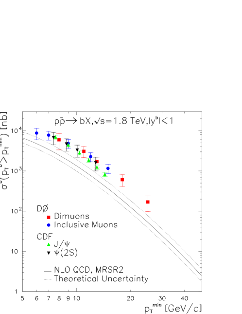
Figure 11: The integrated $p_{T}$ distribution for single $b$ production measured at the Tevatron, and the corresponding QCD prediction.

A similar discrepancy is also observed in UA1 data (see ref. [12] for details).

The theoretical prediction has a considerable uncertainty, which is mainly due to neglected higher-order terms in the perturbative expansion. In our opinion, it is not unlikely that we may have to live with this discrepancy, which is certainly disturbing, but not strong enough to question the validity of perturbative QCD calculations. In other words, the QCD ${\cal O}(\alpha_{\scriptscriptstyle\rm S}^{3})$ corrections for this process are above 100% of the Born term, and thus it is not impossible that higher order terms may give contributions of the same size. Nevertheless, it is useful to look for higher-order perturbative effects and non-perturbative effects that may enhance the cross section.

For values of $p_{T}$ much larger than the $b$ quark mass, large logarithms of the ratio $p_{T}/m_{b}$ arise in the coefficients of the perturbative expansion. Techniques are available to resum this class of logarithms to all orders. In ref. [23] the NLO cross section for the production of a massless parton $i$ (a gluon or a massless quark) has been folded with the NLO fragmentation function for the transition $i\mbox{$\rightarrow$}b$ [24]. The evolution of the fragmentation functions resums all terms of order $\alpha_{\scriptscriptstyle\rm S}^{n}\log^{n}(p_{T}/m_{b})$ and $\alpha_{\scriptscriptstyle\rm S}^{n+1}\log^{n}(p_{T}/m_{b})$. All the dependence on the $b$-quark mass lies in the boundary conditions for the fragmentation function. The result is then matched with the full NLO cross section, which contains the exact dependence on $m_{b}$ up to order $\alpha_{\scriptscriptstyle\rm S}^{3}$, in a way that avoids double counting. Corrections to the result of ref. [23] are either of order $\alpha_{\scriptscriptstyle\rm S}^{4}\log^{i}(p_{T}/m_{b})$, with $i\leq 2$, or of order $\alpha_{\scriptscriptstyle\rm S}^{4}$ times positive powers of $m_{b}/\sqrt{p_{T}^{2}+m_{b}^{2}}$.

Figures 12-13 show the differential and integrated $b$-quark $p_{T}$ distribution obtained in the fragmentation function approach of ref. [23], compared to the standard fixed-order NLO result. It should be noted that for high transverse momenta the scale dependence is significantly reduced with respect to the fixed-order calculation. Furthermore, it can be seen from fig. 13 that, for $10\mathop{\mbox{\vbox{\hbox{$>$} \vskip-9.0pt\hbox{$\sim$} \vskip-3.0pt}}}p_{T}\mathop{\mbox{\vbox{\hbox{$>$} \vskip-9.0pt\hbox{$\sim$} \vskip-3.0pt}}}30$ GeV, the result of the fragmentation-function approach lies slightly above the fixed-order NLO calculation. This has been interpreted in ref. [23] as an evidence for large, positive higher order corrections. Unfortunately, their effect is not easy to quantify. These higher order terms are in fact computed in a massless approximation, and thus fail at low transverse momenta. In figs. 12-13 these terms are suppressed by a factor that becomes smaller and smaller at low $p_{\scriptscriptstyle T}$.

Figure 12: Single-inclusive $p_{T}$ distribution for $b$ production at the Tevatron energy: pure QCD and resummed results.

Figure 13: Integrated $p_{T}$ distribution for $b$ production at the Tevatron energy: pure QCD and resummed results.

A more detailed discussion of this point can be found in the original reference. Here, we simply conclude that some evidence for large higher order terms in the intermediate transverse momentum region is present, although difficult to quantify.

Finally, notice that the overall effect of the inclusion of higher-order logarithms is a steepening of the $p_{T}$ spectrum. This is quite natural, since multiple radiation is accounted for in the resummation procedure.

It has been argued that an intrinsic transverse momentum for the incoming partons may explain the discrepancy observed at the Tevatron. In fact, large values (up to 4 GeV) of the average transverse momentum of the incoming partons have been invoked to explain direct photon production data [25]. Such large values, much larger than typical QCD scales, are clearly incompatible with the usual application of perturbative QCD. Thus, evidence for such a large intrinsic transverse momentum cannot be claimed on the basis of a single observable. In other words, we would need evidence from several observables, all leading to a similar value of the intrinsic $k_{T}$, before we accept such a flaw in the usual perturbative QCD description. Nevertheless, in the following we will perform the exercise of applying very large intrinsic transverse momenta to the heavy flavour production process. This procedure will lead to an increase in the $b$ transverse momentum spectrum. We will also show, however, that other variables, very sensitive to an intrinsic transverse momentum, that should be strongly affected, do not show any evidence of that.

There are several possible ways to implement the presence of a non-zero transverse momentum of the colliding partons, and the choice is, to a large extent, arbitrary. We implemented it in the FMNR code in the following way. We call $\vec{p}_{\scriptscriptstyle\rm T}(Q\overline{Q})$ the total transverse momentum of the pair. For each event, in the longitudinal centre-of-mass frame of the heavy-quark pair, we boost the $Q\overline{Q}$ system to rest. We then perform a transverse boost, which gives the pair a transverse momentum equal to $\vec{p}_{\scriptscriptstyle\rm T}(Q\overline{Q})+\vec{k}_{\scriptscriptstyle\rm T}(1)+\vec{k}_{\scriptscriptstyle\rm T}(2)$; $\vec{k}_{\scriptscriptstyle\rm T}(1)$ and $\vec{k}_{\scriptscriptstyle\rm T}(2)$ are the transverse momenta of the incoming partons, which are chosen randomly, with their moduli distributed according to

$$\frac{1}{N}\frac{dN}{dk_{\scriptscriptstyle\rm T}^{2}}=\frac{1}{\langle k_{\scriptscriptstyle\rm T}^{2}\rangle}\exp(-k_{\scriptscriptstyle\rm T}^{2}/\langle k_{\scriptscriptstyle\rm T}^{2}\rangle).$$ (2)

The reader can find more details in ref. [12].

In fig. 14 we show the effect of an intrinsic $k_{T}$ generated in this way, with the (unphysically large) choice $\langle k_{\scriptscriptstyle\rm T}\rangle=4$  GeV (in fig. 14, the sensitivity to the $\epsilon_{b}$ parameter in the fragmentation function is also shown; fragmentation will be discused in more detail in the next subsection.)

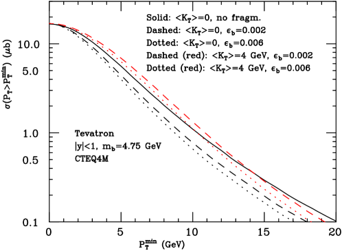
Figure 14: The $b$ cross section at the Tevatron: the effect of a large intrinsic transverse momentum, and the sensitivity to the fragmentation parameter $\epsilon_{b}$.

We see that, for $p_{T}^{min}<20$ GeV, the $k_{T}$ effect is sizeable, even in the presence of fragmentation, provided we allow for unphysically large intrinsic $k_{T}$.

It is fair to ask whether such large values are compatible with other observables. There is a particular class of observables that are particularly sensitive to the intrinsic transverse momentum. One example is the azimuthal distance $\Delta\phi$ between the directions of the produced $b$ and $\overline{b}$. The $\Delta\phi$ distribution is trivial at leading order: $b$ and $\bar{b}$ are emitted back-to-back, and therefore

$$\frac{d\sigma}{d\Delta\phi}\propto\delta(\phi-\pi).$$ (3)

An intrinsic $k_{T}$ of the colliding partons has the effect of smearing the $\delta$ function. For $\langle k_{T}\rangle=4\;$GeV the effect is quite dramatic, as can be seen in fig. 15.

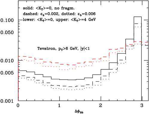
Figure 15: The $b$-$\bar{b}$ azimuthal correlation at the Tevatron: the effect of a large intrinsic transverse momentum, and the sensitivity to the fragmentation parameter $\epsilon_{b}$.

Is such an important effect consistent with the observed azimuth correlations? The CDF and D0 collaborations have measured the azimuthal correlation of muon pairs produced in $b$ decays. In order to compare with these data sets, we have implemented in the FMNR code the semileptonic decay of $b$ quarks. We have assumed that the muon energy is distributed according to the prediction of the spectator model [26] with massless leptons. We have also checked that the muon energy distribution given by Pythia leads to similar results. Our results are shown in figs. 16 and 17, where CDF and D0 data are superimposed to the perturbative QCD prediction, with and without an intrinsic $k_{T}$ with $\langle k_{T}\rangle=4\;$GeV. Tevatron data do not seem to favour such a large intrinsic transverse momentum. The measured distributions are more peaked at $\Delta\phi=\pi$ than the theoretical curve with $\langle k_{T}\rangle=4\;$GeV. The effect of Peterson fragmentation is also shown in both cases.

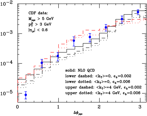
Figure 16: CDF results on azimuthal correlations compared with the perturbative calculation, with and without intrinsic $k_{T}$.

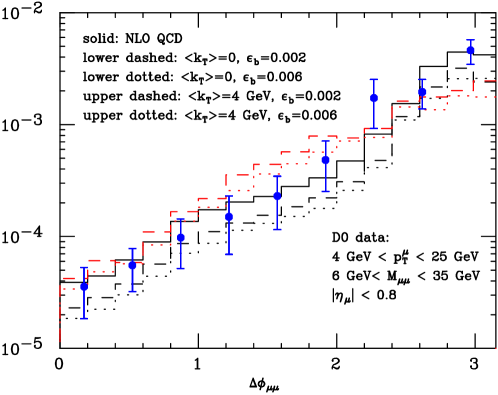
Figure 17: D0 results on azimuthal correlations compared with the perturbative calculation, with and without intrinsic $k_{T}$

We thus conclude that the data does not seem to favour large $k_{T}$ effects.

2.2.3 Single-incusive distributions and correlations at the LHC

In this subsection, we will follow the pragmatic assumption that the discrepancy observed at the Tevatron may either be attributed to a problem in the overall normalization of the cross section, or to the presence of effects, either perturbative or not, that distort the spectrum. We will continue to model these effects as fragmentation effects and intrinsic transverse momentum effects, and see if the LHC can distinguish among the two. In fig. 18 we plot the $b$ cross section with a transverse momentum cut.

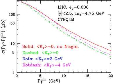
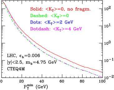
Figure 18: Cross section with a transverse momentum cut at the LHC.

From the figure it is quite clear that the effects of fragmentation and the effects of an intrinsic transverse momentum kick manifest themselves in quite a different way. In particular, at $p_{\scriptscriptstyle T}>20$ GeV even the effect of a very large transverse momentum kick is small, while fragmentation has a strong impact. On the other hand, the transverse momentum kick increases the cross section in the intermediate $p_{\scriptscriptstyle T}$ region, with a maximum around 7 GeV. The $p_{\scriptscriptstyle T}$ coverage offered by the combined LHC experiments will allow an effective discrimination of the two kinds of effects. For completeness, we also show in fig. 19 a comparison of the fixed-order calculation of the single-inclusive spectrum, using the fixed-order calculation in two different schemes for the light flavour, and the matched-resummed result.

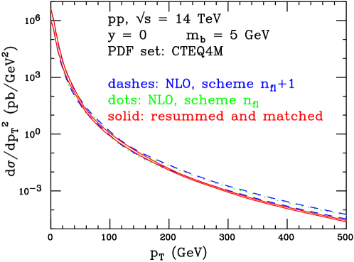
Figure 19: Differential cross section for $b$ production at the LHC. The bands are obtained by varying independently the renormalization and factorization scales by a factor of 2 above and below the central value, which is the $b$ transverse mass.

As in the Tevatron case, the band obtained with the resummation procedure is much narrower at large transverse momentum. The corresponding uncertainty does not include fragmentation function uncertainties, that will be discussed in more detail further on.

As an example of what could be discriminated at the LHC using correlations, we present in fig. 20 the azimuthal correlation of the muons coming from semileptonic $B$ decays, using typical cuts that are implemented in the LHC experiments triggers for $B$ studies.

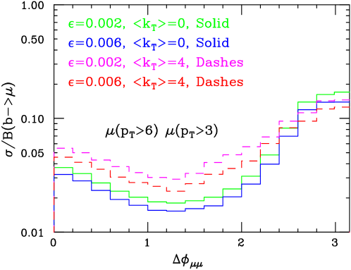
Figure 20: Azimuthal correlations in muon pairs at the LHC.

The curves are obtained with different values of the $\epsilon_{b}$ parameter for the fragmentation function, and with or without a very large intrinsic transverse momentum for the incoming partons. As one can expect, the $\epsilon_{b}$ parameter affects only the total rate in this case, while the primordial transverse momentum has a considerable effect on the shape of the distribution. This example shows that, even with very simple experimental setup, at the LHC it will be possible to test important features of the differential distributions.

2.3 Fragmentation function formalism

In analogy with the case of charm production, the agreement between theory and data improves if one does not include any fragmentation effects. It is then natural to ask whether the fragmentation functions commonly used in these calculations are appropriate. Following the LEP measurements, fragmentation functions have appeared to be harder then previously thought. It will be interesting to see whether SLD new data [27] will help in clarifying this issue.

The effect of a non-perturbative fragmentation function on the $p_{T}$ spectrum is easily quantified if one assumes a steeply-falling transverse momentum distribution for the produced $b$ quark

$$\frac{d\sigma}{dp_{T}}=Ap_{T}^{-M}\,,$$ (4)

The corresponding distribution for the hadron is

$$\frac{d\sigma_{\rm had}}{dp_{T}}=A\int{\hat{p}}_{T}^{-M}\,\delta(p_{T}-z{\hat{p}}_{T})D(z)\,dz\,d{\hat{p}}_{T}=Ap_{T}^{-M}\int_{0}^{1}dzz^{M-1}D(z)\,.$$ (5)

We can see that the hadron spectrum is proportional to the quark spectrum times the $M^{\rm th}$ moment of the fragmentation function $D(z)$. Thus, the larger the moment, the larger the enhancement of the spectrum.

In practice, the value of $M$ will be slightly dependent upon $p_{T}$. We thus define a $p_{T}$ dependent $M$ value

$$\frac{d\log\sigma(p_{T}>p_{T}^{\rm cut})}{d\log p_{T}^{\rm cut}}=-M(p_{T}^{\rm cut})+1$$ (6)

and

$$\sigma_{\rm had}(p_{T}>p_{T}^{\rm cut})=\sigma(p_{T}>p_{T}^{\rm cut})\times\int_{0}^{1}dzz^{M(p_{T}^{\rm cut})-1}D(z)\,.$$ (7)

This gives an excellent approximation to the effect of the fragmentation function, as can be seen from fig. 21.

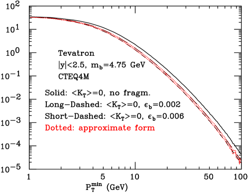
Figure 21: The effect of a Peterson fragmentation function of the inclusive $b$ cross section. The (red) dotted lines correspond to the approximation eq. (6), and are almost indistinguishable from the exact results.

Since the second moment of the fragmentation function is well constrained by $e^{+}e^{-}$ data, it is sensible to ask for what shapes of the fragmentation function, for fixed $\langle z\rangle$, one gets the highest value for $\langle z^{M-1}\rangle$. We convinced ourselves that the maximum is achieved by the functional form

$$D(z)=A\delta(z)+B\delta(1-z)$$ (8)

which gives

$$\langle z\rangle=\frac{B}{A+B}\,;\quad\langle z^{M-1}\rangle=\frac{B}{A+B}\,.$$ (9)

This is however not very realistic: somehow, we expect a fragmentation function which is concentrated at high values of $z$, and has a tail at small $z$. We convinced ourselves that, if we impose the further constraint that $D(z)$ should be monotonically increasing, one gets instead the functional form

$$D(z)=A+B\delta(1-z)\,,$$ (10)

which gives

$$\langle z\rangle=\frac{A/2+B}{A+B}\,;\quad\langle z^{M-1}\rangle=\frac{A/M+B}{A+B}\,.$$ (11)

We computed numerically the $M^{th}$ moments of the Peterson form,

$$D(z)\propto\frac{1}{z\left(1-\frac{1}{z}-\frac{\epsilon}{1-z}\right)^{2}}$$ (12)

of the form

$$D(z)\propto z^{\alpha}(1-z)^{\beta}$$ (13)

for $\beta=1$ (Kartvelishvili), for which

$$\langle z^{M-1}\rangle=\frac{\Gamma(\alpha+M)\Gamma(\alpha+\beta+2)}{\Gamma(\alpha+1)\Gamma(\alpha+\beta+M+1)}\,,$$ (14)

of the form of Collins and Spiller

$$D(z)\propto\frac{\left(\frac{1-z}{z}+\frac{(2-z)\epsilon}{1-z}\right)\left(1+z^{2}\right)}{\left(1-\frac{1}{z}-\frac{\epsilon}{1-z}\right)^{2}}$$ (15)

and of the form in eq. (10), at fixed values of $\langle z\rangle$ corresponding to the choices $\epsilon_{b}=0.002$ and $0.006$ in the Peterson form. We found that the $p_{T}$ distribution at the Tevatron, for $p_{T}$ in the range $10$ to $100$ GeV, behaves like $p_{T}^{-M}$, with $M$ around 5. Therefore, we present in tables 9 and 10 values of the $4^{\rm th}$, $5^{\rm th}$ and $6^{\rm th}$ moments of the above-mentioned fragmentation functions.

Table 9: Values of the $4^{\rm th}$, $5^{\rm th}$ and $6^{\rm th}$ moment, at fixed $\langle z\rangle$ (corresponding to $\epsilon_{b}=0.002$ in the Peterson form), for different forms of the fragmentation function.

$\langle z\rangle=0.879$	$M=4$	$M=5$	$M=6$
Peterson	0.711	0.649	0.595
Kartvelishvili	0.694	0.622	0.562
Collins-Spiller	0.729	0.677	0.633
Maximal (eq. (10))	0.818	0.806	0.798

Table 10: Values of the $4^{\rm th}$, $5^{\rm th}$ and $6^{\rm th}$ moment, at fixed $\langle z\rangle$ (corresponding to $\epsilon_{b}=0.006$ in the peterson form), for different forms of the fragmentation function.

$\langle z\rangle=0.828$	$M=4$	$M=5$	$M=6$
Peterson	0.611	0.535	0.474
Kartvelishvili	0.594	0.513	0.447
Collins-Spiller	0.626	0.559	0.505
Maximal (eq. (10))	0.742	0.724	0.713

We thus find that keeping the second moment fixed the variation of the hadronic $p_{T}$ distribution obtained by varying the shape of the fragmentation function among commonly used models is between 5% and 13% for both values of $\epsilon_{b}$. It thus seems difficult to enhance the transverse momentum distribution by suitable choices of the form of the fragmentation function. With the extreme choice of eq. (10), one gets at most a variation of 50% for the largest value of $\epsilon_{b}$ and $M$. It would be interesting to see if such an extreme choice is compatible with $e^{+}e^{-}$ fragmentation function measurements.

3 A STUDY OF HEAVY QUARK NON-PERTURBATIVE FRAGMENTATION IN HERWIG

In this Section we present the results of a phenomenological study of the non-perturbative hadronization of $b$-quarks. According to the standard QCD picture, distributions for an observable hadron $H$ can be computed by convoluting the short-distance cross section $\hat{\sigma}(p)$ with a fragmentation function $D^{(h)}_{H}(z)$ that describes the way in which the heavy quark $h$ hadronizes into $H$:

$${\rm d}\sigma_{H}(p)=\int dz\,D^{(h)}_{H}(z)\,{\rm d}\hat{\sigma}(p/z).$$ (16)

The precise definition of $D^{(h)}_{H}(z)$ depends on how much of the heavy quark evolution after its production is absorbed into the perturbative part $\hat{\sigma}(p)$, and how much is assigned to the non-perturbative component parameterised by $D^{(h)}_{H}(z)$. Since perturbation theory (PT) is well defined for a massive quark, the standard prescription is to absorb into $\hat{\sigma}(p)$ not only the hard matrix elements, but also the perturbative part of the fragmentation function, defined by the evolution in $Q^{2}$ down to a scale equal to the heavy quark mass $m_{h}$. $D^{(h)}_{H}(z)$ will therefore account for the transition of an “on-shell” quark $h$ into the hadron $H$. The assumptions built into eq. (16) are that $D^{(h)}_{H}(z)$ depends neither on the type of hard process, nor on the scale at which $h$ was produced. Under these assumptions, $D^{(h)}_{H}(z)$ can be extracted from data in one given reaction (typically, $e^{+}e^{-}$), and eventually used to predict the cross section in some other reaction ($p\bar{p}$, DIS and so on).

QCD factorization theorems indicate that this universality of $D^{(h)}_{H}(z)$ holds in the asymptotic limit, and up to corrections of order $m_{h}/Q$, $Q$ being the scale of the hard process. The size of these corrections cannot be calculated, today, in any rigorous way. A possible approach to this problem is to turn to the phenomenological models of hadronization implemented in QCD-based parton-shower Monte Carlo (PSMC) codes. In PSMC the full final-state kinematical configuration is available at both the parton and hadron levels. Therefore, it is possible to “measure” $D^{(h)}_{H}(z)$ using eq. (16), both ${\rm d}\sigma_{H}$ and ${\rm d}\hat{\sigma}$ being known. In the present section, we carry out this program using the PSMC HERWIG [28]. HERWIG evolves quarks according to perturbative QCD down to small scales. The quarks are paired up at the end of the evolution into colour singlet clusters, which are then decayed to the physical hadrons using phenomenological distributions. The study of the heavy quark hadronisation process in HERWIG will allow us to test the universality assumption, and to measure the size of possible deviations.

We should stress that, at this moment, our conclusions are only relevant for the hadronization model implemented in HERWIG; other PSMC’s, which treat the hadronization process differently (for example, by adopting a string model), may well lead to different conclusions.

In order to precisely define our procedure for extracting $D^{(h)}_{H}(z)$, we need to consider in more details the way in which HERWIG generates events. Regardless of the type of initial-state particles, we can distinguish the following steps.

• Hard subprocess: at this stage, the PSMC generates the kinematics for the basic $2\mbox{$\rightarrow$}2$ hard reaction. We denote the momentum of the $b$-quark (or antiquark) as $p_{b}^{hard}$.

• Parton shower: the partons resulting from the hard subprocess undergo successive branchings, until their virtuality is smaller than a fixed cutoff value. We denote the momentum of the $b$-quark at the end of this phase as $p_{b}^{ps}$.

• Gluon splitting and cluster formation: the gluons present at the end of the shower are decayed into light-quark pairs. Colour-singlet, two-body clusters are formed, according to colour parenthood and closeness in the phase-space. If there exist one or more cluster whose mass is too large (relative to a given threshold), part of the cluster rest energy is transformed into new $q\bar{q}$ pairs, and new clusters are defined. In this process, energy-momentum is redistributed among the cluster elements, and the momentum of the $b$-quark can therefore be modified with respect to $p_{b}^{ps}$. The momentum of the $b$ quark after completion of the clustering process will be denoted by $p_{b}^{glsp}$.

• Cluster decay and hadron formation: the clusters decay into observable hadrons, according to the flavour and to tabulated mass spectra. We therefore obtain $b$-flavoured hadrons, whose momentum we denote as $p_{B}$.

The hard subprocess and parton shower stages are based on perturbative QCD. Thus, we identify the predictions given by HERWIG at the end of the parton shower with the cross section $\hat{\sigma}$ that appears in eq. (16). On the other hand, the gluon splitting and cluster decay stages do not contain QCD information, as they are performed according to a phenomenological model. The $g\mbox{$\rightarrow$}q\bar{q}$ splitting and the decay kinematics are induced by simple phase-space considerations. We thus identify these stages as the long-distance, non perturbative part of the process, which gives rise to $D^{(h)}_{H}(z)$. We therefore determine the fragmentation function by comparing the results for $p_{b}^{ps}$ and $p_{B}$, defining, on an event-by-event basis, the following variables:

$$z_{1}=\frac{\vec{p}_{B}\cdot\vec{p}_{b}^{\,ps}}{\left|\vec{p}_{b}^{\,ps}\right|^{2}},\;\;\;\;\;\;z_{2}=\frac{E_{B}+\vec{p}_{B}\cdot\hat{p}_{b}^{\,ps}}{E_{b}^{ps}+\left|\vec{p}_{b}^{\,ps}\right|},$$ (17)

where $\hat{p}_{b}^{\,ps}=\vec{p}_{b}^{\,ps}/\left|\vec{p}_{b}^{\,ps}\right|$. Our conclusions will apply to both $z_{1}$ and $z_{2}$; thus, we will collectively denote them by $z$. In hadronic collisions, the momenta and energies have to be substituted by transverse momenta and transverse energies respectively. Our results are summarized in table 11; we considered $e^{+}e^{-}$ collisions at $\sqrt{S}=91.2$ GeV and $p\bar{p}$ collisions at $\sqrt{S}=1.8$ TeV. In the table, we present four of the (normalized) Mellin moments of the $z$ distribution, defined as follows:

$$\mu_{n}=\int dz\,z^{n}\,D^{(h)}_{H}(z)\,\Big{/}\,\int dz\,D^{(h)}_{H}(z).$$ (18)

Usually, $0\leq z\leq 1$. In the present case, as we will see, we can also have $z>1$; thus, in eq. (18) the range of integration coincide with the support of $D^{(h)}_{H}(z)$.

Table 11: Normalized Mellin moments of the $b$-quark non-perturbative fragmentation function. Results are given for the case of $e^{+}e^{-}$ collisions at $\sqrt{S}=91.2$ GeV and for $p\bar{p}$ collisions at $\sqrt{S}=1.8$ TeV. All numbers have a statistical accuracy of $\pm 0.01$.

	$e^{+}e^{-}$				$p\bar{p}$
	$\mu_{1}$	$\mu_{2}$	$\mu_{3}$	$\mu_{4}$	$\mu_{1}$	$\mu_{2}$	$\mu_{3}$	$\mu_{4}$
$\phantom{10<}\left|\vec{p}_{b}^{\,ps}\right|<5$ GeV	0.87	0.78	0.71	0.66	0.95	0.94	0.94	0.96
$10<\left|\vec{p}_{b}^{\,ps}\right|<15$ GeV	0.92	0.85	0.80	0.76	0.85	0.74	0.66	0.60
$20<\left|\vec{p}_{b}^{\,ps}\right|<25$ GeV	0.92	0.86	0.81	0.76	0.83	0.71	0.63	0.57
$30<\left|\vec{p}_{b}^{\,ps}\right|<35$ GeV	0.92	0.85	0.80	0.75	0.82	0.70	0.62	0.56

The Mellin moments appearing in table 11 have been evaluated by considering bins in $\left|\vec{p}_{b}^{\,ps}\right|$ (in the case of hadronic collisions, the momentum is the transverse one). In $e^{+}e^{-}$ collisions larger (smaller) values of $\left|\vec{p}_{b}^{\,ps}\right|$ correspond to less (more) energy lost to gluons. In hadronic collisions larger (smaller) values of $\left|\vec{p}_{b}^{\,ps}\right|$ are more likely to correspond to larger (smaller) values of the hard process momentum before evolution. In either case, dependence of $D^{(h)}_{H}(z)$ on $\left|\vec{p}_{b}^{\,ps}\right|$ signals therefore a departure from universality.

By inspection of the table, we see that $D^{(h)}_{H}(z)$ is scale-independent to a very good extent (the situation appears to be slightly better in the case of $e^{+}e^{-}$ collisions), except for the very low $p_{b}^{ps}$ region; this is what we should expect, since in that region the factorization theorem on which eq. (16) is based is bound to fail. On the other hand, there seems to emerge a clear difference between the fragmentation functions extracted from $e^{+}e^{-}$ and $p\bar{p}$ “data”, the latter being substantially softer than the former. The first moment, which is the average value of the fragmentation variable, changes by about 10%. This variation can change the rate of predicted $b$-hadrons in hadronic collisions by almost 50%.

This suggests that transporting to hadronic collisions the non-perturbative fragmentation functions obtained by fitting $e^{+}e^{-}$ data may not be correct. Of course, a much more detailed investigation on the subject is required before reaching a firm conclusion; however, this simple exercise of ours shows that universality should not be taken for granted.

We now concentrate on the separate role played in the fragmentation process by the purely perturbative evolution and by the non-perturbative gluon-splitting phase, before the cluster formation and decay take place. We shall confine ourselves to the case of $e^{+}e^{-}$ collisions. The variables relevant to our study are the following:

1. Energy fraction retained during the perturbative evolution:

   $$z_{ps}=\frac{2\left|\vec{p}_{b}^{\,ps}\right|}{\sqrt{S}}=\frac{\left|\vec{p}_{b}^{\,ps}\right|}{\left|\vec{p}_{b}^{\,hard}\right|},$$ (19)

   where $\sqrt{S}$ is the $e^{+}e^{-}$ CM energy.

2. Energy fraction retained during the gluon-splitting:

   $$z_{glsp}=\frac{\left|\vec{p}_{b}^{\,glsp}\right|}{\left|\vec{p}_{b}^{\,ps}\right|}.$$ (20)

3. Energy fraction left after the perturbative evolution and the gluon-splitting:

   $$z=z_{ps}\times z_{glsp}=\frac{2\left|\vec{p}_{b}^{\,glsp}\right|}{\sqrt{S}}=\frac{\left|\vec{p}_{b}^{\,glsp}\right|}{\left|\vec{p}_{b}^{\,hard}\right|},$$ (21)

The left panel in fig. 22 shows the three distributions for $b$ quarks at $\sqrt{S}=91.2$ GeV. The solid histogram represents the distribution of $z_{ps}$. The distribution has the shape of a Gribov-Lipatov, with no indication of a Sudakov turn-over at large $z_{ps}$. The dotted line is the distribution in $z$. A strong deformation of the purely perturbative curve is clearly seen. The dashed line corresponds to the $z_{glsp}$ distribution. This is part of what the MC treats as a non-perturbative component of the fragmentation process. The peak of the dashed histogram at $z_{glsp}=1$ corresponds to events where the cluster containing the heavy quark does not need to be further split, while the tail corresponds to events where the invariant mass of the heavy-quark cluster is too large, and additional light-quark pairs have to be produced by hand. Notice that almost as much energy is lost during this non-perturbative phase, as is lost during the perturbative evolution.

For comparison, we show the same set of curves for the evolution of the charm quark (right panel of fig. 22). Notice that while the effect of the perturbative evolution is to soften the quark spectrum relative to the $b$-quark case, the amount of energy lost due to gluon splitting is similar ($\langle z^{c}_{glsp}\rangle=0.82$, as opposed to $\langle z^{b}_{glsp}\rangle=0.85$). This is bizarre, since one expects the non-perturbative part to scale with $1/m_{h}$. The same result is found for the fragmentation of the $s$ quark (left panel of fig. 23). Here $\langle z^{s}_{glsp}\rangle$ is $0.81$. Again, a violation of the expected $1/m_{h}$ scaling.

Things improve for the top quark, whose distributions for $\sqrt{S}=2$ TeV are shown on the right panel of fig. 23. The gluon-splitting part has only a minor impact on the overall spectrum of the top quark.

We are a bit bothered by the dominant role played by the gluon-splitting phase. By comparison, the next step in the evolution, namely the cluster formation and decay, plays only a minor role, as will be shown next. We would have anticipated that the cluster formation and decay should be the place where most of the non-perturbative physics should show up. This suggests that the thresholds for the perturbative evolution in the MC shold be lowered, so that the impact of the non-perturbative gluon splitting phase is reduced, and purely perturbative Sudakov effects can manifest themselves.

Figure 22: Fragmentation functions for $b$ (left) and $c$ (right) quarks, produced in $e^{+}e^{-}$ collisions at $\sqrt{s}=91.2$ GeV.

Figure 23: Fragmentation functions for $s$ (left) and $t$ (right) quarks, produced in $e^{+}e^{-}$ collisions at $\sqrt{s}=91.2$ (left) and 2000 (right) GeV.

We now turn again to the non-perturbative part of the fragmentation function. The most striking feature, that cannot be inferred from the simple study of Mellin moments as done in table 11, is the presence of a double peak in the high-$z$ region (see the left panel of fig. 24). A first peak (which we will call peak A) is seen at $z$ values around 0.97. A second peak (peak B) is at $z=1.01$ (we have a $z$-bin size of $0.02$. We verified that the events contributing to the peak B do not have $z=1+\epsilon$, i.e., the peak is not due to a roundoff error). The latter peak is higher than the former.

The origin of this double peak can be traced back to the following facts. First, the momentum of the emitted $B$ meson is very strongly correlated with the momentum of the $b$ quark which enters the cluster. Therefore, the $z$ distribution closely reflects the mass spectrum of the light hadron emitted, together with the $B$ meson, in the cluster decay. Second, the peak B is almost entirely due to events where the cluster decay into $B+\pi$: at this peak, $z>1$ because the mass of the pion is lighter than the mass of the lightest quarks in HERWIG. More in detail, we have observed the following facts.

Figure 24: $B$-meson non-perturbative fragmentation function in $e^{+}e^{-}$ at $\sqrt{S}=91.2$ GeV, for 30 GeV$<\left|\vec{p}_{b}\right|<$35 GeV. CLDIR=1, CLSMR=0. See the text for details.

• The structure of the double peak is strongly influenced by the value taken by the two input parameters CLDIR and CLSMR. If the default is used (CLDIR=1, CLSMR=0), the double peak is observed (see the plot on the left of fig.24). On the other hand, by setting CLSMR$\neq$0, the $z$ distributions display a single peak (broader that the previous ones) at about $z=0.97$. For small CLSMR values and large $b$ momenta, a second peak at $z=1.01$ tends to re-appear, although smaller than observed before.

• The double peak disappears also if one chooses CLDIR=0, as in older HERWIG versions. In this case, the $z$ distributions peak at about $z=0.9$, this peak being much broader that those obtained with CLDIR=1, regardless of the value of CLSMR.

• We then set CLDIR=1 and CLSMR=0. For any given $B$ meson, we looked for the parent cluster ${\cal C}=\{b_{C}q\}$, and for the parent bottom quark, $b_{P}$ (the parent quark is defined as in the HERWIG routine HWCHAD). We observed what follows.

  • Plotting the $z$ distributions for the events with $\vec{p}_{b_{C}}\neq\vec{p}_{b_{P}}$ (i.e. events where the original cluster was split), we see a single peak, at the same $z$ value as for the peak A (solid line, plot on the right of fig.24).

  • The $z$ distributions for events such that $\vec{p}_{b_{C}}=\vec{p}_{b_{P}}$ display again a double peak. The two peaks are at the same $z$ values as peaks A and B, the latter one being by far dominant.

  • Selecting only events with $\vec{p}_{b_{C}}=\vec{p}_{b_{P}}$, we found that the peak at the position of B corresponds to those clusters decaying into a $B$ meson and a $\pi$, while the peak at the position of A is relevant for all the other two-body decays (dotted and dashed lines respectively, plot on the right of fig.24).

Overall, notice also that the amount of energy retained after the gluon-splitting phase is of the same size as that retained at the end of the full hadronization process, indicating that cluster formation and decay have a minor impact on the total amount of energy lost during the non-perturbative part of the evolution.

We were also able to reproduce the previous findings with a very simple model. Given a momentum for a quark $b$, we generate randomly the momentum for a light quark $q$, to be combined with $b$ into a cluster, which eventually decays into a $B$ meson and a particle of given mass $m_{P}$. The momentum of the quark $q$ is allowed to have a (small) transverse momentum with respect to the direction of the quark $b$. After evaluating the cluster mass, we performed the decay in the rest frame of the cluster, either in a isotropic manner (thus mimicking the choice CLDIR=0), or by letting the momentum of the meson $B$ to be parallel to that of the quark $b$ (which corresponds to CLDIR=1 and CLSMR=0). In the latter case, depending upon the value of $m_{P}$, we got a peak for $z<1$ (if $m_{P}>m_{q}$) or $z>1$ (if $m_{P}<m_{q}$).

In conclusion, the $z$ distributions we find when using HERWIG seem not to contain a lot of dynamical information, the most important features being those implemented in the cluster-decay routine. If the decay is not smeared out (CLDIR=0), we get a structure which is very difficult to reconcile with the idea of fragmentation we have from QCD. After smearing, the distribution still has a $z>1$ tail which will be extremely difficult to fit with a function vanishing for $z\mbox{$\rightarrow$}1$. This problem is related to the fact that the mass of the lightest quarks in the MC is 320 MeV, that is much larger than the pion mass. We performed a test by reducing the light quark masses to 20 MeV, and increasing the shower cutoff VQCUT in such a way as to maintain the default value of the effective infrared threshold. The double peak structure, as expected, disappeared. It remains to be seen, however, whether such a small value of the quark masses is, more generally, acceptable.

4 A STUDY OF THE $b\overline{b}$ PRODUCTION MECHANISM IN PHYTIA

4.1 Introduction

In this section, we present a study on $b\overline{b}$ production performed within the CMS collaboration using the Monte Carlo package Pythia 5.75 as an event generator. In particular, we investigate the influence of the cut-off on the hard interaction transverse momentum $\hat{P_{t}}$ on the production of $b\overline{b}$ events.

In Monte Carlo programs, $b\overline{b}$ pairs in hadron collisions are produced by the mechanisms of gluon fusion, gluon splitting and flavour excitation. All of them give contributions of the same order to the total cross section, but they give rise to different kinematical configurations of the final state.

There are two ways to generate $b\overline{b}$ events in Pythia:

• Using a steering card MSEL=5, a gluon fusion mechanism ($gg\rightarrow b\overline{b}$) is mainly simulated. Each event contains at least one $b\overline{b}$ pair.

• Using MSEL=1, all QCD $2\rightarrow 2$ processes are simulated. In this case, all production mechanisms contribute to the $b\overline{b}$ production, but the probability to find a $b\overline{b}$ pair in the event is less than 1$\%$.

About one million events have been simulated in CMS with MSEL=1, in order to have a sample with all $b\overline{b}$ production mechanisms and default Pythiacut-off, not to introduce any bias in the kinematics. The selection efficiency of triggered events out of this sample is quite low. In order to have higher signal statistics, in some cases one can use kinematical cuts which are different from the Pythiadefault. [29].

4.2 $b\overline{b}$ production

Two samples have been prepared to investigate the influence of the $\hat{P_{t}}$ cut on the production of $b\overline{b}$ events. Both of them have been generated using MSEL=1 and contain events with only one $b\overline{b}$ pair. Only events with $\hat{P_{t}}\geq 10$ GeV have been selected in the samples. The first sample (SAMPLE A) has been generated with the default $\hat{P_{t}}$ cut of 1 GeV and only events with $\hat{P_{t}}\geq 10$ GeV were selected. The second sample (SAMPLE B) has been generated with $\hat{P_{t}}\geq 10$  GeV. In both samples the following processes contribute:

$$gg\rightarrow q\overline{q}$$ (22)

$$gq_{i}\rightarrow gq_{i}$$ (23)

$$gg\rightarrow gg\;.$$ (24)

$b\overline{b}$ pair is produced by gluon splitting $g\rightarrow b\overline{b}$ in initial or final state shower evolution (processes (22) to (24)) or in the hard interaction (process (22)). For both samples A and B, we have computed the $b\overline{b}$ production cross section

$$\sigma_{b\overline{b}}^{tot}=\frac{N_{b\overline{b}}}{N^{tot}}\sigma^{tot}\;,$$ (25)

where $N_{b\overline{b}}$ is the number of $b\overline{b}$ events with $\hat{P_{t}}\geq 10$ GeV, $N^{tot}$ is the total number of generated events, and $\sigma^{tot}$ is the total cross section (given by Pythia). We find that

• for sample A, $\sigma_{b\overline{b}}^{tot}=150$ $\mu$b. The gluon fusion contribution is about 20 $\mu$b, while the gluon splitting contributions are $\sim 30$ $\mu$b and $\sim 100$ $\mu$b for processes (23) and (24) respectively;

• for sample B, $\sigma_{b\overline{b}}^{tot}$=257 $\mu$b. Gluon fusion and gluon splitting contributions are at the same level as in sample A. In this case, however, there are also contributions from the processes $bg\rightarrow bg$ and $bq\rightarrow bq$ of about 110 $\mu$b. In the following we will call these contributions flavour excitation.

Figure 25 illustrates the difference in the $b\overline{b}$ production cross sections due to the additional contribution of the flavour excitation mechanism in sample B.

Figure 25: Cross section with the two different cut-off on $\hat{P_{t}}$. The solid line is with the default cut-off (1 GeV). The picture is obtained with Pythia 5.75.

The effect has the following explanation. When the default $\hat{P_{t}}$ cut-off is used, Pythia generates processes in the low energy approximation, i.e. there are no heavy quarks inside the parton distribution. This approach changes if one uses a different $\hat{P_{t}}$ cut-off: the parton distributions in this case include also $b$ and $c$ quarks. As a consequence, samples A and B are different in two respects: values of the cross sections, and set of production mechanisms. The difference in the cross section is not very important, because the results are usually normalized to the total $b\overline{b}$ cross section of 500 $\mu$b. On the other hand, the different production mechanisms could be more dangerous, as they can lead to different kinematical distributions, and therefore affect the efficiencies of physical selection.

4.3 Kinematics

The main kinematical parameters which define the signature of $b\overline{b}$ event are the transverse momenta and pseudorapidities of the $b$ quarks, and the angular distance $\Delta\phi$ between their directions in the transverse plane. The first two parameters have similar distributions in both samples. The $\Delta\phi$ distribution is shown in fig. 26 for the three different mechanisms.

Figure 26: Angle between the two $b$ quarks in the transverse plane: the upper one is gluon splitting, the middle is gluon fusion, the last is related to flavour excitation. In the plots the values are not normalized.

For what concerns gluon splitting, the distribution is slightly peaked at small $\Delta\phi$. The angle between the two $b$-quarks produced by the gluon-fusion mechanism has a peak at $\Delta\phi\sim\pi$, as expected, since in the process $gg\rightarrow b\overline{b}$ the b-quarks are produced back-to-back in the transverse plane. The last distribution corresponds to the flavour excitation production mechanism, for which the back-to-back topology is preferred. We can conclude that the total $\Delta\phi$ distributions of sample A and sample B are slightly different. Some care should be taken about this, as it could affect the estimated efficiency of selection cuts.

4.4 Pythia 6.125

We have studied the same problem using the new 6.125 version Pythia. We have generated two new samples A and B with Pythia 6.125, and we have found the following results:

• Sample A: the $b\overline{b}$ production cross section is $\sigma_{b\overline{b}}^{tot}$=220 $\mu$b. Gluon fusion contributes $\sim$ 47 $\mu$b and total gluon splitting gives 173 $\mu$b.

• Sample B: $b\overline{b}$ production cross section is $\sigma_{b\overline{b}}^{tot}$=465 $\mu$b. In this case, gluon fusion is $\sim$ 51 $\mu$b and total gluon splitting is $\sim$ 193 $\mu$b. The contribution from the flavour excitation is about 221 $\mu$b.

Also the way Pythia 6.125 generates $b\overline{b}$ pairs depends on the $\hat{P_{t}}$ cut-off. The difference with Pythia 5.75 values, are due to different total cross section in the two versions.

4.5 Interpretation

Many of the features of Pythia illustrated in this section are easily explained. It turns out that Pythia treats differently processses with a low and high $\hat{p}_{T}^{\rm min}$. The limit is related to the scale of multiple interactions, which is fixed to 2 GeV in the older versions, and was made energy dependent in Pythia 6, being 3.2 GeV at the LHC energy. When $\hat{p}_{T}^{\rm min}$ is above this scale, the hard process is selected according to conventional matrix elements. Below this scale, the hardest interaction is instead taken from the naive jet cross section multiplied by a “Sudakov style” form factor, that represents the probability that higher $p_{T}$ interactions did not take place in the rest of the event. Since this procedure implies the computation of all parton-parton scattering processes, the choice was made to exclude from it the incoming $b$ and $c$ components, to save time in the computation. This feature is no longer considered useful in modern times, the computers being much faster. Thus, in Pythia 6.138, also the $b$ and $c$ processes will be implemented in the low $p_{T}$ mode.

The difference in the total cross section in Pythia 5.7 and 6.1 have a physical origin, since 6.1 uses newer parton distributions that, according to HERA data, are more singular in the small $x$ region.

The authors of Pythia recommend the following procedure for the generation of $b$ events. Parton fusion and flavour excitation can be generated separately; the relevant massive matrix elements are used for parton fusion, and one can go to the limit $p_{T}\mbox{$\rightarrow$}0$ with this process. Gluon splitting cannot be generated separately: all hard processes must be generated, excluding parton fusion and flavour excitation, and one should look for the heavy flavour. Multiple interactions are there switched off, in order to avoid a double-counting of the jet cross section. This is adequate for the study of the $b$ production properties, but clearly does not fully represent the structure of the underlying event. In future Pythia versions, when flavour excitation is included in the minimum bias machinery with multiple interaction, this latter should offer an almost equivalent alternative, but still without the correct mass treatment of the parton fusion process near threshold. Other limitations still remain from complex problems related to the treatment of beam remnants; therefore, flavour excitation is only enabled for the hardest interaction in the multiple-interaction scenario.

A sample of commented code is included below. By using different flags (MEKIND=0,1,2) three samples will be generated: parton fusion, flavour excitation and gluon splitting.

      INTEGER KFINTMP(-40:40)
C... Multiple interactions switched off
      MSTP(81)=0
      PARP(81)=0.D0
      PARP(82)=0.D0
C... Maximum virtuality in ISR is PARP(67)*Q**2
C... This is the default in Pythia 6.137
      PARP(67)=1.D0
C... Choose heavy quark (bottom=5, charm=4)
      MASSIVE=5
C... Helper variable
      HQMASS=PMAS(MASSIVE,1)
C... Choose the kind of heavy quark production:
C... MEKIND is a local variable set to 0, 1 or 2
      IF (MEKIND==0) THEN  ! Massive matrix elements
        MSEL=MASSIVE
      ELSE IF (MEKIND==1) THEN  ! Flavour excitation
        MSEL=1
        CKIN(3)=HQMASS
        CKIN(5)=CKIN(3)
      ELSE IF (MEKIND==2) THEN  ! Gluon splitting (ISR, FSR)
        MSEL=1
        CKIN(3)=HQMASS
        CKIN(5)=CKIN(3)
      END IF
C... More restrictive cuts can be put here.
C... Example, 100 events in total.
      NEVENTS=100
C *** EVENT LOOP ***
      IF (MEKIND==1) NEVENTS=NEVENTS/2
C.... Loop over incoming partons
      DO ISIDE=1,2
        IF (MEKIND/=1.AND.ISIDE==1) THEN
          GOTO 100
        ELSE IF (MEKIND==1) THEN
C... Only for flavour excitation:
C... Make backup copy of KFIN array
          DO IKF=-40,40
            KFINTMP(IKF)=KFIN(ISIDE,IKF)
C... Remove all incoming partons:
            KFIN(ISIDE,IKF)=0
          END DO
C... Select only b/bbar as incoming partons:
          KFIN(ISIDE, MASSIVE)=1
          KFIN(ISIDE,-MASSIVE)=1
        END IF
        DO IEV=1,NEVENTS
C... Generate an event
          CALL PYEVNT
C... For gluon splitting, remove events with HQ in the hard interaction
C... to avoid double counting:
          IF (MEKIND==2) THEN
            DO I=5,8
              IF (ABS(K(I,2))==MASSIVE) GOTO 50
            END DO
          END IF
C... Analysis...
50      END DO
C... Print statistics
      CALL PYSTAT(1)
C... Restore KFIN matrix:
      IF (MEKIND==1.AND.ISIDE==1) THEN
        DO IKF=-40,40
          KFIN(ISIDE,IKF)=KFINTMP(IKF)
        END DO
      END IF
100   END DO

5 ASYMMETRIES

5.1 Introduction

Sizeable leading particle asymmetries between e.g. $\mathrm{D}^{-}$ and $\mathrm{D}^{+}$ have been observed in several fixed target experiments [30]. It is of interest to investigate to what extent these phenomena translate to bottom production and higher energies. No previous experiment has observed asymmetries for bottom hadrons due to limited statistics or other experimental obstacles. Bottom asymmetries are in general expected to be smaller than for charm because of the larger bottom mass, but there is no reason why they should be absent. In the fixed target experiment HERA-B, bottom asymmetries could very well be large [31] even at central rapidities, but the conclusion of the present study is that asymmetries at the LHC are likely to be small. In the following we study possible asymmetries between $\mathrm{B}$ and $\overline{\mathrm{B}}$ hadrons at the LHC within the Lund string fragmentation model [32] and the intrinsic heavy quark model [33].

In the string fragmentation model [34], the perturbatively produced heavy quarks are colour connected to the beam remnants. This gives rise to beam-drag effects where the heavy hadron can be produced at larger rapidities than the heavy quark. The extreme case in this direction is the collapse of a small string, containing a heavy quark and a light beam remnant valence quark of the proton, into a single hadron. This gives rise to flavour correlations which are observed as asymmetries. Thus, in the string model, there can be coalescence between a perturbatively produced bottom quark and a light quark in the beam remnant producing a leading bottom hadron.

There is also the possibility to have coalescence between the light valence quarks and bottom quarks already present in the proton, because the wave function of the proton can fluctuate into Fock configurations containing a $\mathrm{b}\overline{\mathrm{b}}$ pair, such as $|\mathrm{u}\mathrm{u}\mathrm{d}\mathrm{b}\overline{\mathrm{b}}\rangle$. In these states, two or more gluons are attached to the bottom quarks, reducing the amplitude by ${\cal O}(\alpha_{\mathrm{s}}^{2})$ relative to parton fusion [35]. The longest-lived fluctuations in states with invariant mass $M$ have a lifetime of ${\cal O}(2P_{\rm lab}/M^{2})$ in the target rest frame, where $P_{\rm lab}$ is the projectile momenta. Since the comoving bottom and valence quarks have the same rapidity in these states, the heavy quarks carry a large fraction of the projectile momentum and can thus readily combine to produce bottom hadrons with large longitudinal momenta. Such a mechanism can then dominate the hadroproduction rate at large $x_{\mathrm{F}}$. This is the underlying assumption of the intrinsic heavy quark model [33], in which the wave function fluctuations are initially far off shell. However, they materialize as heavy hadrons when light spectator quarks in the projectile Fock state interact with the target [36].

In both models the coalescence probability is largest at small relative rapidity and rather low transverse momentum where the invariant mass of the $\overline{\mathrm{Q}}\mathrm{q}$ system is small, enhancing the binding amplitude. One exception is at very large $p_{\perp}$, where the collapse of a scattered valence quark with a $\overline{\mathrm{b}}$ quark from the parton shower is also possible, giving a further (small) source of leading particle asymmetries in the string model.

5.2 Lund String Fragmentation

Before describing the Lund string fragmentation model, some words on the perturbative heavy quark production mechanisms included in the Monte Carlo event generator Pythia[37] used in this study is in order. We study $\mathrm{p}\mathrm{p}$ events with one hard interaction because events with no hard interaction are not expected to produce heavy flavours and events with more than one hard interaction — multiple interactions — are beyond the scope of this initial study and presumably would not influence the asymmetries. After the hard interaction is generated, parton showers are added, both to the initial (ISR) and final (FSR) state. The branchings in the shower are taken to be of lower virtualities than the hard interaction introducing a virtuality (or time) ordering in the event. This approach gives rise to several heavy quark production mechanisms, which we will call pair creation, flavour excitation and gluon splitting. The names may be somewhat misleading since all three classes create pairs at $\mathrm{g}\mbox{$\rightarrow$}\mathrm{Q}\overline{\mathrm{Q}}$ vertices, but it is in line with the colloquial nomenclature. The three classes are characterized as follows.

Pair creation

The hard subprocess is one of the two LO parton fusion processes $\mathrm{g}\mathrm{g}\mbox{$\rightarrow$}\mathrm{Q}\overline{\mathrm{Q}}$ or $\mathrm{q}\overline{\mathrm{q}}\mbox{$\rightarrow$}\mathrm{Q}\overline{\mathrm{Q}}$. Parton showers do not modify the production cross sections, but only shift kinematics. For instance, in the LO description, the $\mathrm{Q}$ and $\overline{\mathrm{Q}}$ have to emerge back-to-back in azimuth in order to conserve momentum, while the parton shower allows a net recoil to be taken by one or several further partons.

Flavour excitation

A heavy flavour from the parton distribution of one beam particle is put on mass shell by scattering against a parton of the other beam, i.e. $\mathrm{Q}\mathrm{q}\mbox{$\rightarrow$}\mathrm{Q}\mathrm{q}$ or $\mathrm{Q}\mathrm{g}\mbox{$\rightarrow$}\mathrm{Q}\mathrm{g}$. When the $\mathrm{Q}$ is not a valence flavour, it must come from a branching $\mathrm{g}\mbox{$\rightarrow$}\mathrm{Q}\overline{\mathrm{Q}}$ of the parton-distribution evolution. In most current sets of parton-distribution functions, heavy-flavour distributions are assumed to vanish for virtuality scales $Q^{2}<m_{\mathrm{Q}}^{2}$. The hard scattering must therefore have a virtuality above $m_{\mathrm{Q}}^{2}$. When the initial-state shower is reconstructed backwards [38], the $\mathrm{g}\mbox{$\rightarrow$}\mathrm{Q}\overline{\mathrm{Q}}$ branching will be encountered, provided that $Q_{0}$, the lower cutoff of the shower, obeys $Q_{0}^{2}<m_{\mathrm{Q}}^{2}$. Effectively the processes therefore become at least $\mathrm{g}\mathrm{q}\mbox{$\rightarrow$}\mathrm{Q}\overline{\mathrm{Q}}\mathrm{q}$ or $\mathrm{g}\mathrm{g}\mbox{$\rightarrow$}\mathrm{Q}\overline{\mathrm{Q}}\mathrm{g}$, with the possibility of further emissions. In principle, such final states could also be obtained in the above pair-creation case, but the requirement that the hard scattering must be more virtual than the showers avoids double counting.

Gluon splitting

A $\mathrm{g}\mbox{$\rightarrow$}\mathrm{Q}\overline{\mathrm{Q}}$ branching occurs in the initial- or final-state shower but no heavy flavours are produced in the hard scattering. Here the dominant $\mathrm{Q}\overline{\mathrm{Q}}$ source is gluons in the final-state showers since time-like gluons emitted in the initial state are restricted to a smaller maximum virtuality. Except at high energies, most initial state gluon splittings instead result in flavour excitation, already covered above. An ambiguity of terminology exists with initial-state evolution chains where a gluon first branches to $\mathrm{Q}\overline{\mathrm{Q}}$ and the $\mathrm{Q}$ later emits another gluon that enters the hard scattering. From an ideological point of view, this is flavour excitation, since it is related to the evolution of the heavy-flavour parton distribution. From a practical point of view, however, we choose to classify it as gluon splitting, since the hard scattering does not contain any heavy flavours.

In summary, the three classes above are then characterized by having 2, 1 or 0, respectively, heavy flavours in the final state of the LO hard subprocess. Another way to proceed is to add next-to-leading order (NLO) perturbative processes, i.e the $\mathcal{O}(\alpha_{\mathrm{s}}^{3})$ corrections to the parton fusion [3] [4]. However, with our currently available set of calculational tools, the NLO approach is not so well suited for exclusive Monte Carlo studies where hadronization is added to the partonic picture.

Flavour excitation and gluon splitting give significant contributions to the total b cross section at LHC energies and thus must be considered when this is of interest, see the following. However, NLO calculations probably do a better job on the total b cross section itself (while, for the lighter $c$ quark, production in parton showers is so large that the NLO cross sections are more questionable). The shapes of single heavy quark spectra are not altered as much as the correlations between $\mathrm{Q}$ and $\overline{\mathrm{Q}}$ when extra production channels are added. Similar observations have been made when comparing NLO to LO calculations [3] [5]. Likewise, asymmetries between single heavy quarks are also not changed much by adding further production channels, so for simplicity we consider only the pair creation process here.

After an event has been generated at the parton level we add fragmentation to obtain a hadronic final state. We use the Lund string fragmentation model. Its effects on charm production were described in [32]. Here we only summarize the main points.

In the string model, confinement is implemented by spanning strings between the outgoing partons. These strings correspond to a Lorentz-invariant description of a linear confinement potential with string tension $\kappa\approx 1$ GeV/fm. Each string piece has a colour charge at one end and its anticolour at the other. The double colour charge of the gluon corresponds to it being attached to two string pieces, while a quark is only attached to one. A diquark is considered as being in a colour antitriplet representation, and thus behaves (in this respect) like an antiquark. Then each string contains a colour triplet endpoint, a number (possibly zero) of intermediate gluons and a colour antitriplet end. An event will normally contain several separate strings, especially at high energies where $\mathrm{g}\mbox{$\rightarrow$}\mathrm{q}\overline{\mathrm{q}}$ splittings occur frequently in the parton shower.

The string topology can be derived from the colour flow of the hard process with some ambiguity arising from colour-suppressed terms. Consider e.g. the LO process $\mathrm{g}\mathrm{g}\mbox{$\rightarrow$}\mathrm{b}\overline{\mathrm{b}}$ where two distinct colour topologies are possible. Representing the proton remnant by a $\mathrm{u}$ quark and a $\mathrm{u}\mathrm{d}$ diquark (alternatively $\mathrm{d}$ plus $\mathrm{u}\mathrm{u}$), one possibility is to have the three strings $\mathrm{b}$–$\mathrm{u}\mathrm{d}$, $\overline{\mathrm{b}}$–$\mathrm{u}$ and $\mathrm{u}$–$\mathrm{u}\mathrm{d}$, fig. 27, and the other is identical except the $\mathrm{b}$ is instead connected to the $\mathrm{u}\mathrm{d}$ diquark of the other proton because the initial state is symmetric.

Figure 27: Example of a string configuration in a $\mathrm{p}\mathrm{p}$ collision. (a) Graph of the process, with brackets denoting the final colour singlet subsystems. (b) Corresponding momentum space picture, with dashed lines denoting the strings.

Once the string topology has been determined, the Lund string fragmentation model [34] can be applied to describe the nonperturbative hadronization. To first approximation, we assume that the hadronization of each colour singlet subsystem, i.e. string, can be considered separately from that of all the other subsystems. Presupposing that the fragmentation mechanism is universal, i.e. process-independent, the good description of $\mathrm{e}^{+}\mathrm{e}^{-}$ annihilation data should carry over. The main difference between $\mathrm{e}^{+}\mathrm{e}^{-}$ and hadron–hadron events is that the latter contain beam remnants which are colour-connected with the hard-scattering partons.

Depending on the invariant mass of a string, practical considerations lead us to distinguish the following three hadronization prescriptions:

Normal string fragmentation

In the ideal situation, each string has a large invariant mass. Then the standard iterative fragmentation scheme, for which the assumption of a continuum of phase-space states is essential, works well. The average multiplicity of hadrons produced from a string increases linearly with the string ‘length’, which means logarithmically with the string mass. In practice, this approach can be used for all strings above some cutoff mass of a few GeV.

Cluster decay

If a string is produced with a small invariant mass, perhaps only a single two-body final state is kinematically accessible. In this case the standard iterative Lund scheme is not applicable. We call such a low-mass string a cluster and consider its decay separately. When kinematically possible, a $\mathrm{Q}$–$\overline{\mathrm{q}}$ cluster will decay into one heavy and one light hadron by the production of a light $\mathrm{q}\overline{\mathrm{q}}$ pair in the colour force field between the two cluster endpoints with the new quark flavour selected according to the same rules as in normal string fragmentation. The $\overline{\mathrm{q}}$ cluster end or the new $\mathrm{q}\overline{\mathrm{q}}$ pair may also denote a diquark. In the latest version of Pythia, anisotropic decay of a cluster has been introduced, where the mass dependence of the anisotropy has been matched to string fragmentation.

Cluster collapse

This is the extreme case of cluster decay, where the string mass is so small that the cluster cannot decay into two hadrons. It is then assumed to collapse directly into a single hadron which inherits the flavour contents of the string endpoints. The original continuum of string/cluster masses is replaced by a discrete set of hadron masses, mainly $\mathrm{B}$ and $\mathrm{B}^{*}$ (or the corresponding baryon states). This mechanism plays a special rôle since it allows flavour asymmetries favouring hadron species that can inherit some of the beam-remnant flavour contents. Energy and momentum is not conserved in the collapse so that some energy-momentum has to be taken from, or transferred to, the rest of the event. In the new version, a scheme has been introduced where energy and momentum are shuffled locally in an event.

We assume that the nonperturbative hadronization process does not change the perturbatively calculated total rate of bottom production. By local duality arguments [39], we further presume that the rate of cluster collapse can be obtained from the calculated rate of low-mass strings. In the process $\mathrm{e}^{+}\mathrm{e}^{-}\mbox{$\rightarrow$}\mathrm{c}\overline{\mathrm{c}}$ local duality suggests that the sum of the $\mathrm{J}/\psi$ and $\psi^{\prime}$ cross sections approximately equal the perturbative $\mathrm{c}\overline{\mathrm{c}}$ production cross section in the mass interval below the $\mathrm{D}\overline{\mathrm{D}}$-threshold. Similar arguments have also been proposed for $\tau$ decay to hadrons [40] and shown to be accurate. In the current case, the presence of other strings in the event also allows soft-gluon exchanges to modify parton momenta as required to obtain the correct hadron masses. Traditional factorization of short- and long-distance physics would then also preserve the total bottom cross section. Local duality and factorization, however, do not specify how to conserve the overall energy and momentum of an event when a continuum of $\overline{\mathrm{b}}\mathrm{d}$ masses is to be replaced by a discrete $\mathrm{B}^{0}$. In practice, however, the different possible hadronization mechanisms do not affect asymmetries much. The fraction of the string-mass distribution below the two particle threshold effectively determines the total rate of cluster collapse and therefore the asymmetry.

The cluster collapse rate depends on several model parameters. The most important ones are listed here with the Pythia parameter values that we have used. The Pythia parameters are included in the new default parameter set in Pythia 6.135 and later versions.

• Quark masses The quark masses affect the threshold of the string-mass distribution. Changing the quark mass shifts the string-mass threshold relative to the fixed mass of the lightest two-body hadronic final state of the cluster. Smaller quark masses imply larger below-threshold production and an increased asymmetry. The new default masses are PMAS(1)$=m_{\mathrm{u}}=$ PMAS(2)$=m_{\mathrm{d}}=$ 0.33D0, PMAS(3)$=m_{\mathrm{s}}=$ 0.5D0, PMAS(4)$=m_{\mathrm{c}}=$ 1.5D0 and PMAS(5)$=m_{\mathrm{b}}=$ 4.8D0.

• Width of the primordial $k_{\perp}$ distribution. If the incoming partons are given small $p_{\perp}$ kicks in the initial state, asymmetries can appear at larger $p_{\perp}$ since the beam remnants are given compensating $p_{\perp}$ kicks, thus allowing collapses at larger $p_{\perp}$. The new parameters are PARP(91)=1.D0 and PARP(93)=5.D0.

• Beam remnant distribution functions (BRDF). When a gluon is picked out of the proton, the rest of the proton forms a beam remnant consisting, to first approximation, of a quark and a diquark. How the remaining energy and momentum should be split between these two is not known from first principles. We therefore use different parameterizations of the splitting function and check the resulting variations. We find significant differences only at large rapidities where an uneven energy-momentum splitting tend to shift bottom quarks connected to a beam remnant diquark more in the direction of the beam remnant, hence giving rise to asymmetries at very large rapidities. We use an intermediate scenario in this study, given by MSTP(92)=3.

• Threshold behaviour between cluster decay and collapse. Consider a $\mathrm{b}\overline{\mathrm{d}}$ cluster with an invariant mass at, or slightly above, the two particle threshold. Should this cluster decay to two hadrons or collapse into one? In one extreme point of view, a $\mathrm{B}\pi$ pair should always be formed when above this threshold, and never a single $\mathrm{B}$. In another extreme, the two-body fraction would gradually increase at a succession of thresholds: $\mathrm{B}\pi$, $\mathrm{B}^{*}\pi$, $\mathrm{B}\rho$, $\mathrm{B}^{*}\rho$, etc., where the relative probability for each channel is given by the standard flavour and spin mixture in string fragmentation. In our current default model, we have chosen to steer a middle course by allowing two attempts (MSTJ(17)=2) to find a possible pair of hadrons. Thus a fraction of events may collapse to a single resonance also above the $\mathrm{B}\pi$ threshold, but $\mathrm{B}\pi$ is effectively weighted up. If a large number of attempts had been allowed (this can be varied using the free parameter MSTJ(17)), collapse would only become possible for cluster masses below the $\mathrm{B}\pi$ threshold.

The colour connection between the produced heavy quarks and the beam remnants in the string model gives rise to an effect called beam remnant drag. In an independent fragmentation scenario the light cone energy momentum of the quark is simply scaled by some factor picked from a fragmentation function. Thus, on average the rapidity is conserved in the fragmentation process. This is not necessarily so in string fragmentation, where both string ends contribute to the four-momentum of the produced heavy hadron. If the other end of the string is a beam remnant, the hadron will be shifted in rapidity in the direction of the beam remnant resulting in an increase in $|y|$. This beam-drag is shown qualitatively in fig. 28, where the rapidity shift is shown as a function of rapidity and transverse momentum. This shift is not directly accessible experimentally, only indirectly as a discrepancy between the shape of perturbatively calculated quark distributions and the data.

Figure 28: (a) Average rapidity shift $\Delta y=\langle y_{\mathrm{B}}-y_{\mathrm{b}}\rangle$ as a function of $y$ for some different $p_{\perp}$ cuts. (b) Average rapidity shift $\langle|\Delta y|\rangle$ in the direction of “the other end of the string” that the bottom quark is connected to, i.e. ignoring the sign of the shift.

5.3 Intrinsic Heavy Quarks

The wavefunction of a hadron in QCD can be represented as a superposition of Fock state fluctuations, e.g. $|n_{\mathrm{V}}\rangle$, $|n_{\mathrm{V}}\mathrm{g}\rangle$, $|n_{\mathrm{V}}\mathrm{Q}\overline{\mathrm{Q}}\rangle$, …components where $n_{\mathrm{V}}\equiv\mathrm{u}\mathrm{u}\mathrm{d}$ for a proton. When the projectile scatters in the target, the coherence of the Fock components is broken and the fluctuations can hadronize either by uncorrelated fragmentation as for leading twist production or coalescence with spectator quarks in the wavefunction [33] [36]. The intrinsic heavy quark Fock components are generated by virtual interactions such as $\mathrm{g}\mathrm{g}\rightarrow\mathrm{Q}\overline{\mathrm{Q}}$ where the gluons couple to two or more projectile valence quarks. Intrinsic $\mathrm{Q}\overline{\mathrm{Q}}$ Fock states are dominated by configurations with equal rapidity constituents so that, unlike sea quarks generated from a single parton, the intrinsic heavy quarks carry a large fraction of the parent momentum [33].

The frame-independent probability distribution of an $n$–particle $\mathrm{b}\overline{\mathrm{b}}$ Fock state is

$$\frac{dP^{n}_{\rm ib}}{dx_{i}\cdots dx_{n}}=N_{n}\frac{\delta(1-\sum_{i=1}^{n}x_{i})}{(m_{h}^{2}-\sum_{i=1}^{n}(\widehat{m}_{i}^{2}/x_{i}))^{2}}\,\,,$$ (26)

where $\widehat{m}_{i}^{2}=k^{2}_{\perp,i}+m^{2}_{i}$ is the effective transverse mass of the $i^{\rm th}$ particle and $x_{i}$ is the light-cone momentum fraction. The probability, $P^{n}_{\rm ib}$, is normalized by $N_{n}$ and $n=5$ for baryon production from the $|n_{\mathrm{V}}\mathrm{b}\overline{\mathrm{b}}\rangle$ configuration. The delta function conserves longitudinal momentum. The dominant Fock configurations are closest to the light-cone energy shell and therefore the invariant mass, $M^{2}=\sum_{i}\widehat{m}_{i}^{2}/x_{i}$, is minimized. Assuming $\langle\vec{k}_{\perp,i}^{2}\rangle$ is proportional to the square of the constituent quark mass, we choose $\widehat{m}_{\mathrm{q}}=0.45$ GeV, $\widehat{m}_{\mathrm{s}}=0.71$ GeV, and $\widehat{m}_{\mathrm{b}}=5$ GeV [41] [42].

The $x_{\mathrm{F}}$ distribution for a single bottom hadron produced from an $n$-particle intrinsic bottom state can be related to $P^{n}_{\rm ib}$ and the inelastic $\mathrm{p}\mathrm{p}$ cross section by

$$\frac{\sigma^{H}_{\rm ib}(\mathrm{p}\mathrm{p})}{dx_{\mathrm{F}}}=\frac{dP_{H}}{dx_{\mathrm{F}}}\sigma_{\mathrm{p}\mathrm{p}}^{\rm in}\frac{\mu^{2}}{4\widehat{m}_{\mathrm{b}}^{2}}\alpha_{s}^{4}(M_{\mathrm{b}\overline{\mathrm{b}}})\,\,.$$ (27)

The probability distribution is the sum of all contributions from the $|n_{\mathrm{V}}\mathrm{b}\overline{\mathrm{b}}\rangle$ and the $|n_{\mathrm{V}}\mathrm{b}\overline{\mathrm{b}}\mathrm{q}\overline{\mathrm{q}}\rangle$ configurations with $\mathrm{q}=\mathrm{u}$, $\mathrm{d}$, and $\mathrm{s}$ and includes uncorrelated fragmentation and coalescence, as described below, when appropriate [43]. The factor of $\mu^{2}/4\widehat{m}_{\mathrm{b}}^{2}$ arises from the soft interaction which breaks the coherence of the Fock state. We take $\mu^{2}\sim 0.1$ GeV² [44]. The intrinsic charm probability, $P^{5}_{\rm ic}=0.31$%, was determined from analyses of the EMC charm structure function data [45]. The intrinsic bottom probability is scaled from the intrinsic charm probability by the square of the transverse masses, $P_{\rm ib}=P_{\rm ic}(\widehat{m}_{\mathrm{c}}/\widehat{m}_{\mathrm{b}})^{2}$. The intrinsic bottom cross section is reduced relative to the intrinsic charm cross section by a factor of $\alpha_{\mathrm{s}}^{4}(M_{\mathrm{b}\overline{\mathrm{b}}})/\alpha_{\mathrm{s}}^{4}(M_{\mathrm{c}\overline{\mathrm{c}}})$ [46]. Taking these factors into account, we obtain $\sigma^{5}_{\rm ib}(pN)\approx 7$ nb at 14 TeV.

There are two ways of producing bottom hadrons from intrinsic $\mathrm{b}\overline{\mathrm{b}}$ states. The first is by uncorrelated fragmentation. If we assume that the $\mathrm{b}$ quark fragments into a $\mathrm{B}$ meson, the $\mathrm{B}$ distribution is

$$\frac{dP^{nF}_{\rm ib}}{dx_{\mathrm{B}}}=\int dz\prod_{i=1}^{n}dx_{i}\frac{dP^{n}_{\rm ib}}{dx_{1}\ldots dx_{n}}\frac{D_{B/b}(z)}{z}\delta(x_{\mathrm{B}}-zx_{\mathrm{b}})\,\,,$$ (28)

These distributions are assumed for all intrinsic bottom production by uncorrelated fragmentation with $D_{H/b}(z)=\delta(z-1)$. At low $p_{\perp}$, this approximation should not be too bad, as seen in fixed target production [42].

If the projectile has the corresponding valence quarks, the bottom quark can also hadronize by coalescence with the valence spectators. The coalescence distributions are specific for the individual bottom hadrons. It is reasonable to assume that the intrinsic bottom Fock states are fragile and can easily materialize into bottom hadrons in high-energy, low momentum transfer reactions through coalescence. The coalescence contribution to bottom hadron production is

$$\frac{dP^{nC}_{\rm ib}}{dx_{H}}=\int\prod_{i=1}^{n}dx_{i}\frac{dP^{n}_{\rm ib}}{dx_{1}\ldots dx_{n}}\delta(x_{H}-x_{H_{1}}-\cdots-x_{H_{n_{\mathrm{V}}}})\,\,.$$ (29)

where the coalescence function is simply a delta function combining the momentum fractions of the quarks in the Fock state configuration that make up the valence quarks of the final-state hadron.

Not all bottom hadrons can be produced from the minimal intrinsic bottom Fock state configuration, $|n_{\mathrm{V}}\mathrm{b}\overline{\mathrm{b}}\rangle$. However, coalescence can also occur within higher fluctuations of the intrinsic bottom Fock state. For example, in the proton, the $\mathrm{B}^{-}$ and $\Xi_{\mathrm{b}}^{0}$ can be produced by coalescence from $|n_{\mathrm{V}}\mathrm{b}\overline{\mathrm{b}}\mathrm{u}\overline{\mathrm{u}}\rangle$ and $|n_{\mathrm{V}}\mathrm{b}\overline{\mathrm{b}}\mathrm{s}\overline{\mathrm{s}}\rangle$ configurations. These higher Fock state probabilities can be obtained using earlier results on $\psi\psi$ pair production [47] [48]. If all the measured $\psi\psi$ pairs [49] arise from $|n_{\mathrm{V}}\mathrm{c}\overline{\mathrm{c}}\mathrm{c}\overline{\mathrm{c}}\rangle$ configurations, $P_{\rm icc}\approx 4.4\%\ P_{\rm ic}$ [48] [50]. It was found that the probability of a $|n_{\mathrm{V}}\mathrm{c}\overline{\mathrm{c}}\mathrm{q}\overline{\mathrm{q}}\rangle$ state was then $P_{\rm icq}=(\hat{m}_{\mathrm{c}}/\hat{m}_{\mathrm{q}})^{2}P_{\rm icc}$ [47]. If we then assume $P_{\rm ibq}=(\hat{m}_{\mathrm{c}}/\hat{m}_{\mathrm{b}})^{2}P_{\rm icq}$, we find that

$$P_{\rm ibq}\approx\left(\frac{\widehat{m}_{\mathrm{c}}}{\widehat{m}_{\mathrm{b}}}\right)^{2}\left(\frac{\widehat{m}_{\mathrm{c}}}{\widehat{m}_{\mathrm{q}}}\right)^{2}P_{\rm icc}\,\,,$$ (30)

leading to $P_{\rm ibu}=P_{\rm ibd}\approx 70.4\%\ P_{\rm ib}$ and $P_{\rm ibs}\approx 28.5\%\ P_{\rm ib}$. To go to still higher configurations, one can make similar assumptions. However, as more partons are included in the Fock state, the coalescence distributions soften and approach the fragmentation distributions, eventually producing bottom hadrons with less momentum than uncorrelated fragmentation from the minimal $\mathrm{b}\overline{\mathrm{b}}$ state if a sufficient number of $\mathrm{q}\overline{\mathrm{q}}$ pairs are included. There is then no longer any advantage to introducing more light quark pairs into the configuration—the relative probability will decrease while the potential gain in momentum is not significant. Therefore, we consider production by fragmentation and coalescence from the minimal state and the next higher states with $\mathrm{u}\overline{\mathrm{u}}$, $\mathrm{d}\overline{\mathrm{d}}$ and $\mathrm{s}\overline{\mathrm{s}}$ pairs.

The probability distributions entering Eq. (27) for $\mathrm{B}^{0}$ and $\overline{\mathrm{B}}^{0}$ are

$$\frac{dP_{\mathrm{B}^{0}}}{dx_{\mathrm{F}}} = \frac{1}{2}\left(\frac{1}{10}\frac{dP_{\rm ib}^{5F}}{dx_{\mathrm{F}}}+\frac{1}{4}\frac{dP_{\rm ib}^{5C}}{dx_{\mathrm{F}}}\right)+\frac{1}{2}\left(\frac{1}{10}\frac{dP_{\rm ibu}^{7F}}{dx_{\mathrm{F}}}+\frac{1}{5}\frac{dP_{\rm ibu}^{7C}}{dx_{\mathrm{F}}}\right)$$ (31)

$$+\,\frac{1}{2}\left(\frac{1}{10}\frac{dP_{\rm ibd}^{7F}}{dx_{\mathrm{F}}}+\frac{2}{5}\frac{dP_{\rm ibd}^{7C}}{dx_{\mathrm{F}}}\right)+\frac{1}{2}\left(\frac{1}{10}\frac{dP_{\rm ibs}^{7F}}{dx_{\mathrm{F}}}+\frac{1}{5}\frac{dP_{\rm ibs}^{7C}}{dx_{\mathrm{F}}}\right)$$

$$\frac{dP_{\overline{\mathrm{B}}^{0}}}{dx_{\mathrm{F}}} = \frac{1}{10}\frac{dP_{\rm ib}^{5F}}{dx_{\mathrm{F}}}+\frac{1}{10}\frac{dP_{\rm ibu}^{7F}}{dx_{\mathrm{F}}}+\frac{1}{2}\left(\frac{1}{10}\frac{dP_{\rm ibd}^{7F}}{dx_{\mathrm{F}}}+\frac{1}{8}\frac{dP_{\rm ibd}^{7C}}{dx_{\mathrm{F}}}\right)+\frac{1}{10}\frac{dP_{\rm ibs}^{7F}}{dx_{\mathrm{F}}}\,\,.$$ (32)

See Ref. [43] for more details and the probability distributions of other bottom hadrons.

5.4 Model predictions

In this section we present some results from both models. Figure 29 shows the asymmetry between $\mathrm{B}^{0}$ and $\overline{\mathrm{B}}^{0}$ as a function of $y$ for several $p_{\perp}$ cuts in the string model. The asymmetry is essentially zero for central rapidities and increases slowly with rapidity. When the kinematical limit is approached, the asymmetry changes sign for small $p_{\perp}$ because of the drag-effect since $\mathrm{b}$-quarks are often connected to diquarks from the proton beam remnant, fig. 27, thus producing $\overline{\mathrm{B}}^{0}$ hadrons which are shifted more in rapidity than $\mathrm{B}^{0}$. Cluster collapse, on the other hand, tend to enhance the production of leading particles (in this case $\mathrm{B}^{0}$) so the two mechanisms give rise to asymmetries with different signs. Collapse is the main effect at small rapidities while eventually at very large $y$, the drag effect dominates.

Figure 29: The asymmetry, $A=\frac{\sigma(\mathrm{B}^{0})-\sigma(\overline{\mathrm{B}}^{0})}{\sigma(\mathrm{B}^{0})+\sigma(\overline{\mathrm{B}}^{0})}$, as a function of rapidity for different $p_{\perp}$ cuts: (a) $p_{\perp}<5,10$ GeV and (b) $p_{\perp}>5,10$ GeV using parameter set 1 as described in the text.

In Table 12 we study the parameter dependence of the asymmetry by looking at the integrated asymmetry for different kinematical regions using three different parameter sets:

• Set 1 is the new default as presented in section 5.2.

• Set 2 The same as Set 1 except it uses simple counting rules in the beam remnant splitting, i.e. each quark get on average one third of the beam remnant energy-momentum.

• Set 3 The old parameter set, before fitting to fixed-target data, is included as a reference. This set is characterized by current algebra masses, lower intrinsic $k_{\perp}$, and an uneven sharing of beam remnant energy-momentum.

We see that in the central region the asymmetry is generally very small whereas for forward (but not extremely forward) rapidities and moderate $p_{\perp}$ the asymmetry is around 1–2%. In the very forward region at small $p_{\perp}$, drag asymmetry dominates which can be seen from the change in sign of the asymmetry. The asymmetry is fairly stable under moderate variations in the parameters even though the difference between the old and new parameter sets (Set 1 and 3) are large in the central region. Set 1 typically gives rise to smaller asymmetries.

Table 12: Parameter dependence of the asymmetry in the string model. The statistical error in the last digit is shown in parenthesis (95% confidence).

Parameters	$|y|<2.5$, $p_{\perp}>5$ GeV	$3<|y|<5$, $p_{\perp}>5$ GeV	$|y|>3$, $p_{\perp}<5$ GeV
Set 1	0.003(1)	0.015(2)	$-$0.008(1)
Set 2	$-$0.000(2)	0.009(3)	$-$0.005(2)
Set 3	0.013(2)	0.020(3)	$-$0.018(2)

The cross sections for all intrinsic bottom hadrons are given as a function of $x_{\mathrm{F}}$ in fig. 30. The bottom baryon distributions are shown in fig. 30(a). The $\Lambda_{\mathrm{b}}^{0}$ ($\Sigma_{\mathrm{b}}^{0}$) distributions are the largest and most forward peaked of all the distributions. The $\Sigma_{\mathrm{b}}^{-}$ is the smallest and the softest, similar to that of the bottom-strange mesons and baryons shown in fig. 30(b). The different coalescence probabilities assumed for hadrons from the $|\mathrm{u}\mathrm{u}\mathrm{d}\mathrm{b}\overline{\mathrm{b}}\mathrm{s}\overline{\mathrm{s}}\rangle$ configuration have little real effect on the shape of the cross section, dominated by independent fragmentation. Of the $\mathrm{B}$ mesons shown in fig. 30(c), the $\mathrm{B}^{+}$ and $\mathrm{B}^{0}$ cross sections are the largest since both can be produced from the 5 particle configuration. The $\mathrm{B}^{-}$ and $\overline{\mathrm{B}}^{0}$ distributions are virtually identical. We note that the $x_{\mathrm{F}}$ distributions of other bottom hadrons not included in the figure would be similar to the bottom-strange hadrons since they would be produced by fragmentation only.

Figure 30: Predictions for bottom hadron production are given for $\mathrm{p}\mathrm{p}$ collisions at 14 TeV. The bottom baryon distributions are given in (a) for $\Lambda_{\mathrm{b}}^{0}=\Sigma_{\mathrm{b}}^{0}$ (dot-dashed), $\Sigma_{\mathrm{b}}^{+}$ (dashed), and $\Sigma_{\mathrm{b}}^{-}$ (solid). The bottom-strange distributions are shown in (b) for $\Xi_{\mathrm{b}}^{0}$ (solid), $\Xi_{\mathrm{b}}^{-}$ (dashed), $\mathrm{B}_{\mathrm{s}}^{0}$ (dot-dashed), and $\overline{\mathrm{B}}_{s}^{0}$ (dotted). In (c), the $\mathrm{B}$ meson distributions are given: $\mathrm{B}^{+}$ (solid), $\mathrm{B}^{-}$ (dashed), $\mathrm{B}^{0}$ (dot-dashed), and $\overline{\mathrm{B}}^{0}$ (dotted). The $\mathrm{B}^{-}$ and $\overline{\mathrm{B}}^{0}$ distributions are virtually identical.

The $x_{\mathrm{F}}$ distribution for final-state hadron $H$ is the sum of the leading-twist fusion and intrinsic bottom components,

$$\frac{d\sigma^{H}_{hN}}{dx_{\mathrm{F}}}=\frac{d\sigma^{H}_{\rm lt}}{dx_{\mathrm{F}}}+\frac{d\sigma^{H}_{\rm ib}}{dx_{\mathrm{F}}}\,\,.$$ (33)

The intrinsic bottom cross sections from Section 5.3 are combined with a leading twist calculation using independent fragmentation where drag effects are not included. The leading twist results have been smoothed and extrapolated to large $x_{\mathrm{F}}$ to facilitate a comparison with the intrinsic bottom calculation. The resulting total $\mathrm{B}^{0}$ and $\overline{\mathrm{B}}^{0}$ distributions are shown in fig. 31, along with the corresponding asymmetry. Note that since the intrinsic heavy quark $p_{\perp}$ distributions are more steeply falling than the leading twist, we only consider $p_{\perp}<5$ GeV. The distributions are drawn to emphasize the high $x_{\mathrm{F}}$ region where the distributions differ. The asymmetry is $\sim 0.1$ at $x_{\mathrm{F}}\sim 0.25$, corresponding to $y\sim 6.5$. Therefore, intrinsic bottom should not be a significant source of asymmetries.

Figure 31: (a) Leading-twist predictions for $\mathrm{B}^{0}$ (solid) and $\overline{\mathrm{B}}^{0}$ (dashed) using independent fragmentation. Model predictions for $\mathrm{B}^{0}$ (dot-dashed) and $\overline{\mathrm{B}}^{0}$ (dotted) distributions from Eq. (33). (b) The asymmetry between $\mathrm{B}^{0}$ and $\overline{\mathrm{B}}^{0}$, the dot-dashed and dotted curves in (a), is also given.

5.5 Summary

To summarize, we have studied possible production asymmetries between $\mathrm{b}$ and $\overline{\mathrm{b}}$ hadrons, especially $\mathrm{B}^{0}$ and $\overline{\mathrm{B}}^{0}$, as predicted by the Lund string fragmentation model and the intrinsic heavy quark model. We find negligible asymmetries for central rapidities and large $p_{\perp}$ (in general, less than 1%). For some especially favoured kinematical ranges such as $y>3$ and $5<p_{\perp}<10$ GeV the collapse asymmetry could be as high as 1–2%. Intrinsic bottom becomes important only for $x_{\mathrm{F}}>0.25$ and $p_{\perp}<5$ GeV, corresponding to $y>6.5$.

6 QUARKONIUM PRODUCTION

The production of charmonium and bottomonium states at high-energy colliders has been the subject of considerable interest during the past few years. New experimental results from $p\bar{p}$, $ep$ and $e^{+}e^{-}$ colliders have become available, some of which revealed dramatic shortcomings of earlier quarkonium production models. In theory, progress has been made on the factorization between the short distance physics of heavy-quark creation and the long-distance physics of bound state formation. The colour-singlet model [51] [52] has been superseded by a consistent and rigorous framework, based on the use of non-relativistic QCD (NRQCD) [53], an effective field theory that includes the so-called colour-octet mechanisms. On the other hand, the colour evaporation model [54] [55] [56] of the early days of quarkonium physics has been revived [57] [58] [59] [60]. However, despite the recent theoretical and experimental developments the range of applicability of the different approaches is still subject to debate, as is the quantitative verification of factorization. Because the quarkonium mass is still not very large with respect to the QCD scale, in particular for the charmonium system, non-factorizable corrections [61] [62] [63] may not be suppressed enough, if the quarkonium is not part of an isolated jet, and the expansions in NRQCD may not converge very well. In this situation a global analysis of various processes is mandatory in order to assess the importance of different quarkonium production mechanisms, as well as the limitations of a particular theoretical framework (for reviews on different quarkonium production processes see e.g. [64] [65] [66].) By the time the LHC starts operating, new experimental data from the Tevatron and HERA as well as theoretical progress, e.g. in the calculation of higher-order corrections, will have significantly improved the present picture and will allow more precise predictions than what is possible at present. In the following, we will therefore focus on the general phenomenological implications of the NRQCD approach for quarkonium production at the LHC, rather than aiming at a detailed and comprehensive numerical analysis. Based on the information provided by the present Tevatron data we will derive predictions for observables crucial for future LHC analyses, such as differential cross sections and quarkonium polarization.

In the NRQCD approach, the cross section for producing a quarkonium state $H$ at a hadron collider can be expressed as a sum of terms, each of which factors into a short-distance coefficient and a long-distance matrix element:

$$\mbox{d}\sigma(pp/p\bar{p}\mbox{$\rightarrow$}H+X)=\sum_{n}\mbox{d}\hat{\sigma}(pp/p\bar{p}\mbox{$\rightarrow$}Q\overline{Q}\,[n]+x)\,\langle{\cal{O}}^{H}\,[n]\rangle,$$ (34)

where $n$ denotes the colour, spin and angular momentum state of an intermediate $Q\overline{Q}$ pair. The short-distance cross section $\mbox{d}\hat{\sigma}$ can be calculated perturbatively in the strong coupling $\alpha_{s}$. The NRQCD matrix elements $\langle{\cal O}^{H}[n]\rangle$ (see [53] for their definition) are related to the non-perturbative transition probabilities from the $Q\overline{Q}$ state $n$ into the quarkonium $H$. They scale with a definite power of the intrinsic heavy-quark velocity $v$ [67]. ($v^{2}\sim 0.3$ for charmonium and $v^{2}\sim 0.1$ for bottomonium.) The general expression (34) is thus a double expansion in powers of $\alpha_{s}$ and $v$.

The NRQCD formalism implies that so-called colour-octet processes associated with higher Fock state components of the quarkonium wave function must contribute to the cross section. Heavy quark pairs that are produced at short distances in a colour-octet state can evolve into a physical quarkonium through radiation of soft gluons at late times in the production process, when the quark pair has already expanded to the quarkonium size. Such a possibility is ignored in the colour-singlet model, where only those heavy quark pairs that are produced in the dominant Fock state (i.e. in a colour-singlet state and with the spin and angular momentum quantum numbers of the meson) are assumed to form a physical quarkonium. The most profound theoretical evidence that the colour-singlet model is incomplete comes from the presence of infrared divergences in the production cross sections and decay rates of $P$-wave states. Within the NRQCD approach, this problem finds its natural solution since the infrared singularities are factored into a colour-octet operator matrix element [68]. While colour-octet contributions are needed for a consistent description of $P$-wave quarkonia, they are phenomenologically even more important for $S$-wave states like $J/\psi$ or $\Upsilon$. According to the velocity scaling rules, colour-octet matrix elements for the production of $S$-wave quarkonia are suppressed by a factor $v^{4}$ compared to the leading colour-singlet contributions. However, as discussed in some detail below, colour-octet processes can become significant if the short-distance cross section for producing $Q\overline{Q}$ in a colour-octet state is enhanced.

The production of $S$-wave charmonium in $p\bar{p}$ collisions at the Tevatron has attracted considerable attention and has stimulated much of the recent theoretical development in quarkonium physics. The CDF collaboration has measured cross sections for the production of $J/\psi$ and $\psi(2S)$ states not coming from $B$ or radiative $\chi$ decays, for a wide range of transverse momenta $5\,\mbox{GeV}\;\hbox to0.0pt{\lower 3.5pt\hbox{$\mathchar 0\relax\sim$}\hss}\raise 1.0pt\hbox{$<$}\;p_{t}(\psi)\;\hbox to0.0pt{\lower 3.5pt\hbox{$\mathchar 0\relax\sim$}\hss}\raise 1.0pt\hbox{$<$}\;20\,\mbox{GeV}$ [69] [70]. Surprisingly, the experimental cross sections were found to be orders of magnitudes larger than the theoretical expectation based on the leading-order colour-singlet model [71] [72]. This result is particularly striking because the data extends out to large transverse momenta where the theoretical analysis is rather clean. The shortcoming of the colour-singlet model can be understood by examining a typical Feynman diagram contributing to the leading-order parton cross section, fig. 32(a).

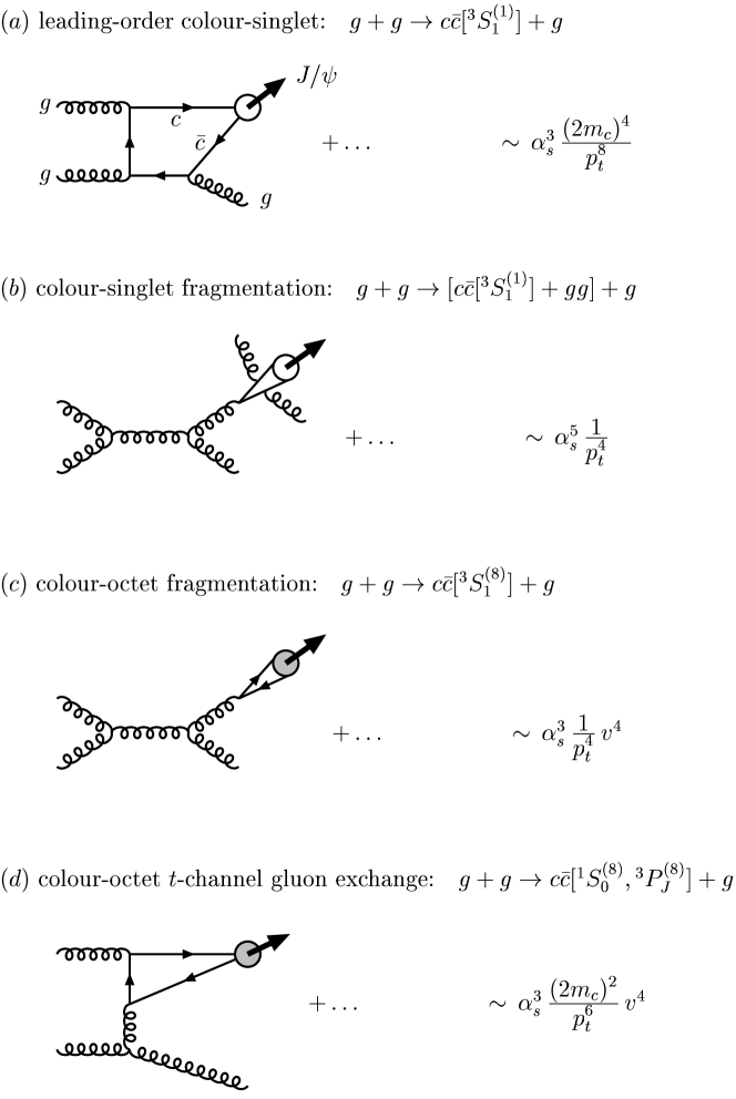
Figure 32: Generic diagrams for $J/\psi$ production in hadron-hadron collisions via colour-singlet and colour-octet channels.

At large transverse momentum, the two internal quark propagators are off-shell by $\sim p_{t}^{2}$ so that the parton differential cross section scales like $\mbox{d}\sigma/\mbox{d}p_{t}^{2}\sim 1/p_{t}^{8}$, as indicated in the figure. On the other hand, when $p_{t}\gg 2m_{c}$ the quarkonium mass can be considered small and the inclusive charmonium cross section is expected to scale like any other single-particle inclusive cross section $\sim 1/p_{t}^{4}$. The dominant production mechanism for charmonium at sufficiently large $p_{t}$ must thus be via fragmentation [73], the production of a parton with large $p_{t}$ which subsequently decays into charmonium and other partons. A typical fragmentation contribution to colour-singlet $J/\psi$ production is shown in fig. 32(b). While the fragmentation contributions are of higher order in $\alpha_{s}$ compared to the fusion process fig. 32(a), they are enhanced by a power $p_{t}^{4}/(2m_{c})^{4}$ at large $p_{t}$ and can thus overtake the fusion contribution at $p_{t}\gg 2m_{c}$. When colour-singlet fragmentation is included, the $p_{t}$ dependence of the theoretical prediction is in agreement with the Tevatron data but the normalization is still underestimated by about an order of magnitude [74] [75] [76], indicating that an additional fragmentation contribution is still missing. It is now generally believed that gluon fragmentation into colour-octet ${}^{3}S_{1}$ charm quark pairs [77] [78], as shown in fig. 32(c), is the dominant source of $J/\psi$ and $\psi(2S)$ at large $p_{t}$ at the Tevatron. The probability of forming a $J/\psi$ particle from a pointlike $c\bar{c}$ pair in a colour-octet ${}^{3}S_{1}$ state is given by the NRQCD matrix element $\langle{\cal O}^{J/\psi}[{}^{3}S_{1}^{(8)}]\rangle$ which is suppressed by $v^{4}$ relative to the non-perturbative factor of the leading colour-singlet term. However, this suppression is overcompensated for by the gain in two powers of $\alpha_{s}/\pi$ in the short-distance cross section for producing colour-octet ${}^{3}S_{1}$ charm quark pairs as compared to colour-singlet fragmentation. At ${\cal{O}}(v^{4})$ in the velocity expansion, two additional colour-octet channels have to be included, fig. 32(d), which do not have a fragmentation interpretation at order $\alpha_{s}^{3}$ but which become significant at moderate $p_{t}\sim 2m_{c}$ [79] [80]. The importance of the ${}^{1}S_{0}^{(8)}$ and ${}^{3}P_{J}^{(8)}$ contributions cannot be estimated from naive power counting in $\alpha_{s}$ and $v$ alone, but rather follows from the dominance of $t$-channel gluon exchange, forbidden in the leading-order colour-singlet cross section.

The different contributions to the $J/\psi$ transverse momentum distribution are compared to the CDF data [70] in fig. 33.

Figure 33: Colour-singlet and colour-octet contributions to direct $J/\psi$ production in $p\bar{p}\mbox{$\rightarrow$}J/\psi+X$ at the Tevatron ($\sqrt{s}=1.8$ TeV, pseudorapidity cut $|\eta|<0.6$)) together with experimental data from CDF [70]. Parameters: CTEQ5L parton distribution functions [81]; factorization and renormalization scale $\mu=\sqrt{p_{t}^{2}+4m_{c}^{2}}$; $m_{c}=1.5$ GeV. The leading logarithms $(\alpha_{s}\ln p_{t}^{2}/(2m_{c})^{2})^{n}$ have been summed by solving the Altarelli-Parisi evolution equations for the gluon fragmentation function. NRQCD matrix elements as specified in Table 13.

Table 13: NRQCD matrix elements for charmonium production. The colour-singlet matrix elements are taken from the potential model calculation of [82] [83]. The colour-octet matrix elements have been extracted from the CDF data [70], where $M_{k}^{H}(^{1}\!S_{0}^{(8)},^{3}\!P_{0}^{(8)})\equiv\langle{\cal O}_{8}^{H}[{}^{1}S_{0}]\rangle+k\,\langle{\cal O}_{8}^{H}[{}^{3}P_{0}]\rangle/m_{c}^{2}$. The errors quoted are statistical only. Parameters: CTEQ5L parton distribution functions [81], renormalization and factorization scale $\mu=(p_{t}^{2}+4m_{c}^{2})^{1/2}$ and $m_{c}=1.5\,$GeV. The Altarelli-Parisi evolution has been included for the ${}^{3}S_{1}^{(8)}$ fragmentation contribution. See [84] for further details.

$$\begin{array}[]{cccc}\hline\cr\hline\cr H&\langle{\cal{O}}_{1}^{H}\rangle&\langle{\cal{O}}_{8}^{H}[{}^{3}S_{1}]\rangle&M_{3.5}^{H}({}^{1}S_{0}^{(8)},{}^{3}P_{0}^{(8)})\\ \hline\cr J/\psi&1.16~{}{\rm GeV^{3}}&(1.19\pm 0.14)\cdot 10^{-2}~{}{\rm GeV}^{3}&(4.54\pm 1.11)\cdot 10^{-2}~{}{\rm GeV}^{3}\\[-2.84526pt] \psi(2S)&0.76~{}{\rm GeV^{3}}&(0.50\pm 0.06)\cdot 10^{-2}~{}{\rm GeV}^{3}&(1.89\pm 0.46)\cdot 10^{-2}~{}{\rm GeV}^{3}\\[-2.84526pt] \chi_{0}&0.11~{}{\rm GeV^{5}}&(0.31\pm 0.04)\cdot 10^{-2}~{}{\rm GeV}^{3}&\\ \hline\cr\hline\cr\end{array}$$

As mentioned above, the colour-singlet model at lowest order in $\alpha_{s}$ fails dramatically when confronted with the experimental results. When colour-singlet fragmentation is included, the prediction increases by more than an order of magnitude at large $p_{t}$, but it still falls below the data by a factor of $\sim 30$. The CDF results on charmonium production can be explained by including the leading colour-octet contributions and adjusting the unknown non-perturbative parameters to fit the data. Numerically one finds the non-perturbative matrix elements to be of ${\cal{O}}(10^{-2}~{}\mbox{GeV}^{3})$, see Table 13, perfectly consistent with the $v^{4}$ suppression expected from the velocity scaling rules. Similar conclusions can be drawn for $\psi(2S)$ production at the Tevatron.

The analysis of the CDF data alone, although very encouraging, does not strictly prove the phenomenological relevance of colour-octet contributions because free parameters have to be introduced to fit the data. However, if factorization holds the non-perturbative matrix elements, Table 13, are universal and can be used to make predictions for various processes and observables. Besides a global analysis of different reactions, the measurement of quarkonium cross sections at the LHC will be crucial to assess the importance of the individual production mechanisms and to test factorization. In fig. 34 we have collected the cross section predictions for direct $J/\psi$ and $\psi(2S)$ production as well as the production of $J/\psi$ from radiative $\chi$ decays at the LHC.

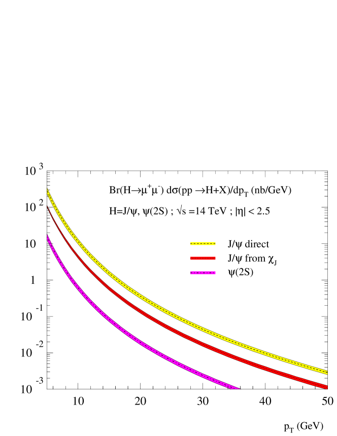
Figure 34: Cross sections for $J/\psi$ and $\psi(2S)$ production in $pp\mbox{$\rightarrow$}\psi+X$ at the LHC ($\sqrt{s}=14$ TeV, pseudorapidity cut $|\eta|<2.5$). Parameter specifications as in fig. 33. The leading logarithms $(\alpha_{s}\ln p_{t}^{2}/(2m_{c})^{2})^{n}$ have been summed by solving the Altarelli-Parisi evolution equations for the gluon fragmentation function. The error bands include the statistical errors in the extraction of the NRQCD matrix elements [Table 13] only.

The theoretical curves include the statistical errors in the extraction of the NRQCD matrix elements [Table 13]. There are, however, additional theoretical uncertainties which might affect the prediction, but which have not yet been fully quantified. In particular the determination of the $\langle{\cal O}_{8}^{\psi}[{}^{1}S_{0}]\rangle$ and $\langle{\cal O}_{8}^{\psi}[{}^{3}P_{0}]\rangle$ matrix elements ($\psi$ denoting $J/\psi$ or $\psi(2S)$) from the Tevatron data is very sensitive to effects that modify the shape of the charmonium $p_{t}$ distribution at relatively small $p_{t}\;\hbox to0.0pt{\lower 3.5pt\hbox{$\mathchar 0\relax\sim$}\hss}\raise 1.0pt\hbox{$<$}\;8$ GeV. Those effects include the small-$x$ behaviour of the gluon distribution [84], the evolution of the strong coupling [84], as well as systematic effects inherent in NRQCD, such as the inaccurate treatment of the energy conservation in the hadronization of the colour-octet $c\bar{c}$ pairs [85]. Moreover, higher-order QCD corrections are expected to play an important role, as discussed in more detail below. The cross sections collected in fig. 34 should thus not be viewed as firm NRQCD predictions but will be refined as more experimental and theoretical information on charmonium production becomes available over the next few years.

The inclusion of higher-order QCD corrections is required to reduce the theoretical uncertainty and to allow a more precise prediction of the LHC cross sections. Next-to-leading order (NLO) calculations for quarkonium production at hadron colliders are presently available only for total cross sections [86] [87]. Significant higher-order corrections to differential distributions are expected from the strong renormalization and factorization scale dependence of the leading-order results [85]. Moreover, the NLO colour-singlet cross section includes processes like $g+g\mbox{$\rightarrow$}Q\overline{Q}[{}^{3}S_{1}^{(1)}]+g+g$ which are dominated by $t$-channel gluon exchange and scale as $\sim\alpha_{s}^{4}(2m_{Q})^{2}/p_{t}^{6}$. At $p_{t}\gg 2m_{Q}$ their contribution is enhanced with respect to the the leading-order cross section, fig. 32(a), which scales as $\sim\alpha_{s}^{3}(2m_{Q})^{4}/p_{t}^{8}$. This is born out by preliminary studies [88] which include part of the NLO hadroproduction cross section and by the complete calculation of NLO corrections to the related process of quarkonium photoproduction [89]. The NLO colour-singlet cross section may be comparable in size to the colour-octet ${}^{1}S_{0}$ and ${}^{3}P_{J}$ processes, which scale as $\sim\alpha_{s}^{3}v^{4}(2m_{Q})^{2}/p_{t}^{6}$ (see fig. 32(d)), and affect the determination of the corresponding NRQCD matrix elements from the Tevatron data. A full NLO analysis is however needed before quantitative conclusions can be drawn.

Another source of potentially large higher-order corrections is the multiple emission of soft or almost collinear gluons from the initial state partons. These corrections, as well as effects related to intrinsic transverse momentum, are expected to modify the shape of the transverse momentum distribution predominantly at relatively low values of $p_{t}\;\hbox to0.0pt{\lower 3.5pt\hbox{$\mathchar 0\relax\sim$}\hss}\raise 1.0pt\hbox{$<$}\;2m_{Q}$. Initial state radiation can be partially summed in perturbation theory [90], but so far only total cross sections have been considered in the literature [91]. An estimate of the effect on the transverse momentum distribution should be provided by phenomenological models where a Gaussian $k_{t}$-smearing is added to the initial state partons. The result of these calculations not only depends on the average $\langle k_{t}\rangle$, which enters as a free parameter, but also on the details of how the smearing is implemented. Moreover, a lower cut-off has to be provided which regulates the divergences at $p_{t}=0$. Using the NLO calculation for the total cross section [87], one can obtain the rough estimate that perturbative Sudakov effects should be confined below $p_{t}\sim 1-2$ GeV for both charmonium and bottomonium production at Tevatron energies. Qualitatively, the inclusion of $k_{t}$-smearing leads to an enhancement of the short distance cross section at small $p_{t}$, which results in smaller values for the fits of the $\langle{\cal O}_{8}^{\psi}[{}^{1}S_{0}]\rangle$ and $\langle{\cal O}_{8}^{\psi}[{}^{3}P_{0}]\rangle$ NRQCD matrix elements [92] [88]. The actual size of the effect, however, turns out to be very different for the two models studied in the literature.

An alternative approach to treat the effect of initial state radiation is by means of Monte Carlo event generators which include multiple gluon emission in the parton shower approximation. Comprehensive phenomenological analyses have been carried out for charmonium production at the Tevatron and at the LHC [93] [94] [95] using the event generator Pythia [37] supplemented by the leading colour-octet processes [93]. The inclusion of initial state radiation as implemented in Pythia leads to an enhancement of the short-distance cross section. The size of the effect is significantly larger than for the Gaussian $k_{t}$-smearing mentioned above, and it extents out to large $p_{t}$. Consequently, the $\langle{\cal O}_{8}^{\psi}[{}^{1}S_{0}]\rangle$ and $\langle{\cal O}_{8}^{\psi}[{}^{3}P_{0}]\rangle$ NRQCD matrix elements estimated from the Monte Carlo analysis of the Tevatron cross sections are significantly lower than the ones listed in Table 13 (see [93] [94] for details). Figure 35 shows the individual contributions to the direct $J/\psi$ cross section at the LHC as estimated with the Pythia Monte Carlo [94].

Figure 35: Cross sections for $J/\psi$ production in $pp\mbox{$\rightarrow$}J/\psi+X$ at the LHC ($\sqrt{s}=14$ TeV, rapidity cut $|y|<2.5$) obtained from a Monte Carlo event generator [94]. CTEQ2L parton distribution functions [99]; (i) dotted line: colour-singlet, (ii) dashed line: colour-octet ${}^{1}S_{0}+{}^{3}P_{J}$, (iii) dot-dashed line: ${}^{3}S_{1}^{(8)}$, (iv) solid line: all contributions. NRQCD matrix elements as specified in [94].

Note that for consistency the curves are based on the NRQCD matrix elements extracted from the Monte Carlo analysis of the Tevatron data rather than on the values of the leading-order fit listed in Table 13. One observes that the final prediction is consistent with the result presented in fig. 34 within errors. The extrapolation of the Tevatron fits to LHC energies seems rather insensitive to the details of the underlying theoretical description, and different approaches yield similar predictions for the LHC cross sections as long as the appropriate NRQCD matrix elements are used. The Monte Carlo implementation [93] should therefore represent a convenient and reliable tool for the experimental simulation of quarkonium production processes at the LHC.

A crucial test of the NRQCD approach to charmonium production at hadron colliders is the analysis of $J/\psi$ and $\psi(2S)$ polarization at large transverse momentum. Recall that at large $p_{t}$, $\psi$ production should be dominated by gluon fragmentation into a colour-octet ${}^{3}S_{1}$ charm quark pair, fig. 32(c). When $p_{t}\gg 2m_{c}$ the fragmenting gluon is effectively on-shell and transverse. The intermediate $c\bar{c}$ pair in the colour-octet ${}^{3}S_{1}$ state inherits the gluon’s transverse polarization and so does the quarkonium, because the emission of soft gluons during hadronization does not flip the heavy quark spin at leading order in the velocity expansion. Consequently, at large transverse momentum one should observe transversely polarized $J/\psi$ and $\psi(2S)$ [100]. The polarization can be measured through the angular distribution in the decay $\psi\mbox{$\rightarrow$}l^{+}l^{-}$, given by $\mbox{d}\Gamma/\mbox{d}\!\cos\theta\propto 1+\alpha\,\cos^{2}\theta$, where $\theta$ denotes the angle between the lepton three-momentum in the $\psi$ rest frame and the $\psi$ three-momentum in the lab frame. Pure transverse polarization implies $\alpha=1$. Corrections to this asymptotic limit due to spin-symmetry breaking and higher order fragmentation contributions have been estimated to be small [101]. The dominant source of depolarization comes from the colour-octet fusion diagrams, fig. 32(d), which are important at moderate $p_{t}$. Still, at ${\cal{O}}(v^{4})$ in the velocity expansion, the polar angle asymmetry $\alpha$ can be unambiguously calculated within NRQCD [84] [102] in terms of the three non-perturbative matrix elements [Table 13] that have been determined from the unpolarized cross section. In fig. 36 we display the theoretical prediction for $\alpha$ in $\psi(2S)$ production at the Tevatron as function of the $\psi(2S)$ transverse momentum.

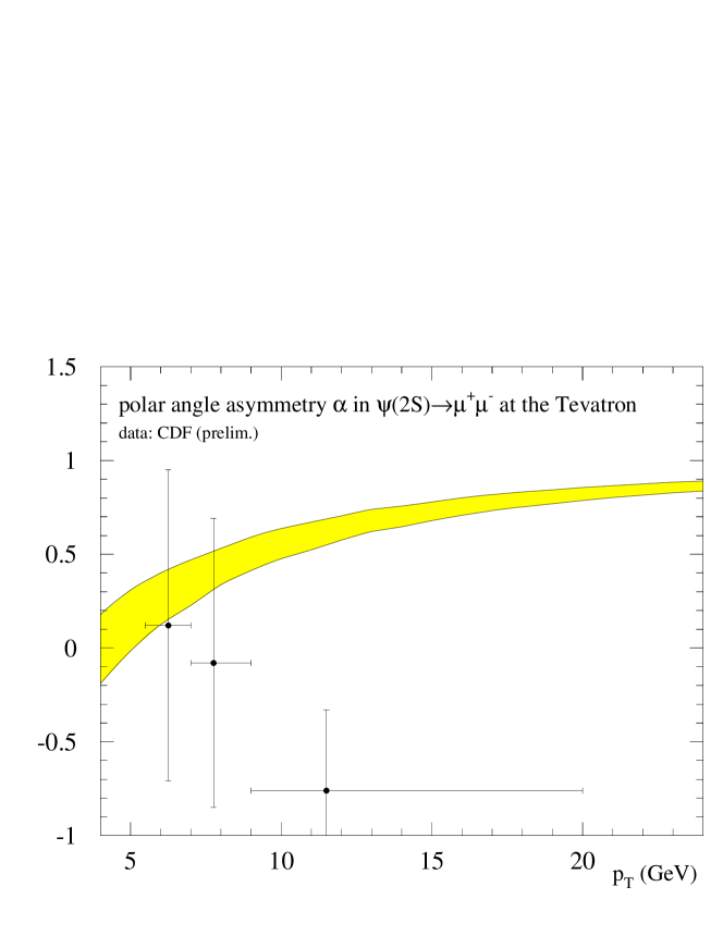
Figure 36: Polar angle asymmetry $\alpha$ for $\psi(2S)$ production in $p\bar{p}\mbox{$\rightarrow$}\psi(2S)(\mbox{$\rightarrow$}\mu^{+}\mu^{-})+X$ at the Tevatron as a function of $p_{t}$ compared to preliminary data from CDF [103]. Parameter specifications as in fig. 33. NLO corrections to the fragmentation contribution [101] [84] have not been included. The error band is obtained as a combination of the uncertainty (statistical only) in the extraction of the NRQCD matrix elements [Table 13] and the limiting cases that either $\langle{\cal O}_{8}^{\psi}({}^{1}S_{0})\rangle$ or $\langle{\cal O}_{8}^{\psi}({}^{3}P_{0})\rangle$ is set to zero in the linear combination extracted from the data.

No transverse polarization is expected at $p_{t}\sim 5\,$ GeV, but the angular distribution is predicted to change drastically as $p_{t}$ increases. A preliminary measurement from CDF [103] does not support this prediction, but the experimental errors are too large to draw definite conclusions. A similar picture emerges from the analysis of $J/\psi$ polarization [104], where, however, the theoretical analysis is complicated by the fact that the data sample still includes $J/\psi$ that have not been produced directly but come from decays of higher excited states [105].

Polarization measurements are crucial to discriminate the NRQCD approach from the colour evaporation model, where the cross section for a specific charmonium state is given as a universal fraction of the inclusive $c\overline{c}$ production cross section integrated up to the open charm threshold. In general, the assumption of a single universal long-distance factor is too restrictive. It implies a universal $\sigma(\chi_{c})/\sigma(J/\psi)$ ratio, which is not supported by the comparison of charmonium production in hadron-hadron and photon-hadron collisions. Still, since the colour evaporation model allows colour-octet charm quark pairs from gluon fragmentation to hadronize into charmonium, it can describe the $p_{t}$ distribution of the Tevatron data [57] [58] [59] [60]. In contrast to the NRQCD approach, however, the colour evaporation model predicts charmonium to be produced unpolarized. The model assumes unsuppressed gluon emission from the $c\bar{c}$ pair during hadronization which randomizes spin and colour. This assumption is clearly wrong in the heavy quark limit where spin symmetry is at work and soft gluon emission does not flip the heavy quark spin. Nonetheless, since the charm quark mass is not very large with respect to the QCD scale, the applicability of heavy quark spin symmetry to charmonium physics has to be tested by confronting the NRQCD polarization signature with experimental data.

To definitely resolve the issue of quarkonium polarization, a high-statistics measurement extending out to large transverse momentum will be necessary. Such a measurement can be carried out at the LHC, where one expects a polarization pattern similar to that predicted for the Tevatron, see fig. 37.

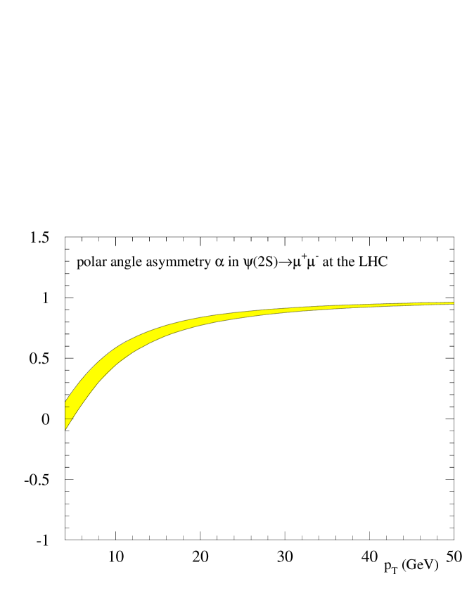
Figure 37: Polar angle asymmetry $\alpha$ for $\psi(2S)$ production in $pp\mbox{$\rightarrow$}\psi(2S)(\mbox{$\rightarrow$}\mu^{+}\mu^{-})+X$ at the LHC as a function of $p_{t}$. Parameter specifications as in fig. 36.

The absence of a substantial fraction of transverse polarization in $\psi$ production at large $p_{t}$ would represent a serious problem for the application of the NRQCD factorization approach to the charmonium system and might indicate that the charm quark mass is not large enough for a nonrelativistic approach to work in all circumstances.

The application of NRQCD should be on safer grounds for the bottomonium system. As $v^{2}\sim 0.1$ for bottomonium, higher-order terms in the velocity expansion (in particular colour-octet contributions) are expected to be less relevant than in the case of charmonium. Cross sections for the production of $\Upsilon$ states have been measured at the Tevatron in the region $p_{t}\;\hbox to0.0pt{\lower 3.5pt\hbox{$\mathchar 0\relax\sim$}\hss}\raise 1.0pt\hbox{$<$}\;20\,\mbox{GeV}$ [106] [107] [108]. The leading-order colour-singlet model predictions underestimate the data, the discrepancy being, however, much less significant than in the case of charmonium. Given the large theoretical uncertainties in the cross section calculation, in particular at small $p_{t}\;\hbox to0.0pt{\lower 3.5pt\hbox{$\mathchar 0\relax\sim$}\hss}\raise 1.0pt\hbox{$<$}\;M_{\Upsilon}$, the need for colour-octet contribution is not yet as firmly established as for charmonium production. The inclusion of both next-to-leading order corrections and the summation of soft gluon radiation is required to obtain a realistic description of the $\Upsilon$ cross section in the $p_{t}$-range probed by present data. Such calculations have not yet been performed, and we have therefore not attempted a systematic fit [79] [80] of the bottomonium NRQCD matrix elements. Our predictions for the $\Upsilon$ cross section at the LHC, figs. 38,39, are based on a simple choice of the non-perturbative input parameters [Table 14] which is consistent with the present experimental information from the Tevatron.

Table 14: NRQCD matrix elements for bottomonium production. The colour-singlet matrix elements are taken from the potential model calculation of [82] [83]. The colour-octet matrix elements have been determined from the CDF data for $p_{t}>8~{}{\rm GeV}$ [107], where $\langle{\cal O}_{8}^{H}[{}^{1}S_{0}]\rangle=\langle{\cal O}_{8}^{H}[{}^{3}P_{0}]\rangle/m_{b}^{2}$ has been assumed for simplicity. Parameters: CTEQ5L parton distribution functions [81], renormalization and factorization scale $\mu=(p_{t}^{2}+4m_{b}^{2})^{1/2}$ and $m_{b}=4.88\,$GeV.

$$\begin{array}[]{cccc}\hline\cr\hline\cr H&\langle{\cal{O}}_{1}^{H}\rangle&\langle{\cal{O}}_{8}^{H}[^{3}S_{1}]\rangle&\langle{\cal{O}}_{8}^{H}[^{1}S_{0}]\rangle\\ \hline\cr\Upsilon(1S)&9.28~{}{\rm GeV^{3}}&15\cdot 10^{-2}~{}{\rm GeV}^{3}&2.0\cdot 10^{-2}~{}{\rm GeV}^{3}\\[-2.84526pt] \Upsilon(2S)&4.63~{}{\rm GeV^{3}}&4.5\cdot 10^{-2}~{}{\rm GeV}^{3}&0.6\cdot 10^{-2}~{}{\rm GeV}^{3}\\[-2.84526pt] \Upsilon(3S)&3.54~{}{\rm GeV^{3}}&7.5\cdot 10^{-2}~{}{\rm GeV}^{3}&1.0\cdot 10^{-2}~{}{\rm GeV}^{3}\\[-2.84526pt] \chi_{0}(1P)&2.03~{}{\rm GeV^{5}}&4.0\cdot 10^{-2}~{}{\rm GeV}^{3}\\[-2.84526pt] \chi_{0}(2P)&2.57~{}{\rm GeV^{5}}&6.5\cdot 10^{-2}~{}{\rm GeV}^{3}\\ \hline\cr\hline\cr\end{array}$$

The cross sections should thus not be regarded as firm predictions of NRQCD but rather as order-of-magnitude estimates. The expected theoretical progress and more experimental information will allow a more precise prediction in the near future.

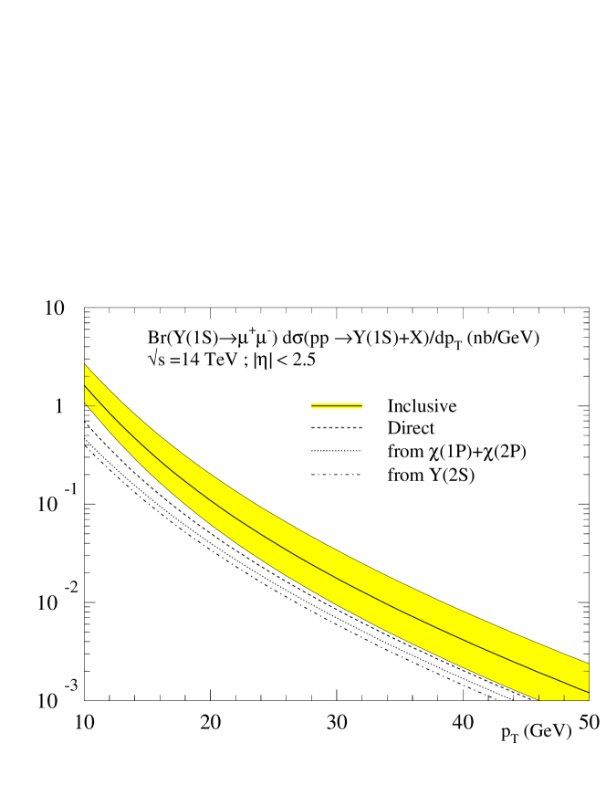
Figure 38: Cross sections for $\Upsilon(1S)$ production in $pp\mbox{$\rightarrow$}\Upsilon(1S)+X$ at the LHC ($\sqrt{s}=14$ TeV, pseudorapidity cut $|\eta|<2.5$). Parameters: CTEQ5L parton distribution functions [81], factorization and renormalization scale $\mu=\sqrt{p_{t}^{2}+4m_{b}^{2}}$, $m_{b}=4.88$ GeV. The leading logarithms $(\alpha_{s}\ln p_{t}^{2}/(2m_{b})^{2})^{n}$ have been summed by solving the Altarelli-Parisi evolution equations for the gluon fragmentation function. NRQCD matrix elements as specified in Table 14. The error band is obtained by varying the colour-octet matrix elements between half and twice their central value for illustration.

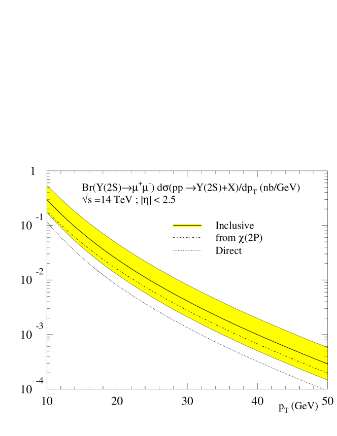
Figure 39: Same as fig. 38 for $\Upsilon(2S)$ production.

The impact of initial state gluon radiation on the $\Upsilon$ cross sections at the Tevatron has been estimated by adding a Gaussian $k_{t}$-smearing as discussed previously in the context of charmonium production. An average $\langle k_{t}\rangle\sim 3$ GeV and a $K$-factor $\sim 3$ are found to bring the leading-order colour-singlet cross section in line with the experimental $\Upsilon(1S,2S)$ data at $p_{t}\;\hbox to0.0pt{\lower 3.5pt\hbox{$\mathchar 0\relax\sim$}\hss}\raise 1.0pt\hbox{$<$}\;M_{\Upsilon}$ [109]. Similar results have been obtained within a Monte Carlo analysis [110], leading to significantly lower fit values for the colour-octet NRQCD matrix elements than those determined from a leading-order calculation [Table 14]. Moreover, the Monte Carlo results imply that no feeddown from $\chi$ states produced through colour-octet ${}^{3}S_{1}$ $b\bar{b}$ states is needed to describe the inclusive $\Upsilon$ cross section, in contrast to what is found at leading-order. The calculation of next-to-leading order corrections and a systematic treatment of soft gluon radiation within perturbation theory are required to resolve these issues. Figure 40 shows the inclusive $\Upsilon(1S)$ cross section at the LHC as obtained from the Monte Carlo calculation [110].

Figure 40: Cross sections for $\Upsilon(1S)$ production in $pp\mbox{$\rightarrow$}\Upsilon(1S)+X$ at the LHC ($\sqrt{s}=14$ TeV, rapidity cut $|y|<2.5$) obtained from a Monte Carlo event generator [110]. CTEQ2L parton distribution functions [99]; (i) dot-dashed line: ${}^{3}S_{1}^{(8)}$, (ii) solid line: all contributions. NRQCD matrix elements as specified in [110].

The curves are based on the NRQCD matrix elements extracted from the Monte Carlo analysis of the Tevatron data [110]. As in the case of charmonium production, one observes that the final LHC prediction is consistent with the leading-order result presented in fig. 38 within errors.

Let us finally present the polarization pattern predicted for direct $\Upsilon(1S)$ production at the LHC, fig. 41, based on the NRQCD matrix elements of Table 14.

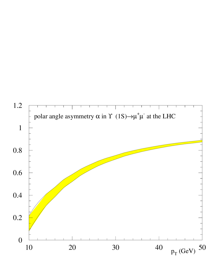
Figure 41: Polar angle asymmetry $\alpha$ for direct $\Upsilon(1S)$ production in $pp\mbox{$\rightarrow$}\Upsilon(1S)(\mbox{$\rightarrow$}\mu^{+}\mu^{-})+X$ at the LHC as a function of $p_{t}$. NRQCD matrix elements as specified in Table 14 other parameters as in Figure 38. The error band reflects the limiting cases that either $\langle{\cal O}_{8}^{\psi}({}^{1}S_{0})\rangle$ or $\langle{\cal O}_{8}^{\psi}({}^{3}P_{0})\rangle$ is set to zero in the linear combination extracted from the data.

Higher-order corrections to the gluon fragmentation function [101] [84] will lead to a small reduction of the transverse polarization at large $p_{t}$ and should be included once precise data become available. If the charmonium mass is indeed not large enough for a nonrelativistic expansion to be reliable, the onset of transverse $\Upsilon$ polarization at $p_{t}\gg M_{\Upsilon}$ may become the single most crucial test of the NRQCD factorization approach.

In summary, we have discussed some of the phenomenological implications of the NRQCD approach for quarkonium production at the LHC and presented ’state-of-the-art’ predictions for $\psi$ and $\Upsilon$ differential cross sections and polarization. Among the theoretical issues that need to be addressed in the future are the calculation of higher-order QCD corrections, the summation of higher-order terms in the velocity expansion and quantitative insights in the effect of higher-twist contributions. Besides a global analysis of different production processes and observables at various colliders, quarkonium physics at the LHC will play a crucial role to assess the importance of colour-octet processes and to conclusively test the applicability of non-relativistic QCD and heavy-quark spin symmetry to the charmonium and bottomonium systems.

7 PROSPECTS FOR $b$ PRODUCTION MEASUREMENTS AT THE LHC

Of the existing and currently proposed accelerator facilities, the LHC will yield the largest rate of $b$ quarks. A well defined program for $b$ production investigations, and the development of dedicated detection strategies optimised for ATLAS, CMS and LHCb, are required for the succesful exploitation of the rich LHC potential. After an introduction summarising the main physics motivations, we review the detector and trigger features relevant for $b$ production in the LHC experiments. The kinematic ranges accessible to the three experiments are then described. Theoretical motivations and possible measurement methods are presented for single $b$ quark properties, correlations in $b$ production, multiple heavy flavour production, polarization, and charge asymmetry effects in $B$-hadron production in $pp$ interactions. Based on earlier performance studies, the potential for these measurements is estimated and some preliminary results are presented. We conclude with a summary of the present status of the preparations for $b$-production studies.

7.1 Introduction

While many LHC studies have been devoted to $B$-decays, $b$ production has not yet been directly addressed. Even though $b$ decay investigations will provide some information on the production, at the discussions of this workshop it became clear that they are not sufficient to cover all aspects of production.

Heavy quark production in high energy hadronic collisions is important for the study of Quantum Chromodynamics (QCD). Nowadays, QCD is recognized as a well established and solid theory. If disagreements between the theoretical predictions and the experimental data are found, they will suggest the lack of understanding only of a particular production mechanism. In many cases these disagreements may be attributed to a too slow convergence of the perturbation series. In other cases, there may be important contributions from nonperturbative effects. Strictly speaking, the production measurements are not going to test the principles of QCD, but rather to outline the boundaries, where the predictions of perturbation theory provide an adequate description and exhaust all the visible effects. In this context, it will be certainly useful to test as many different processes as possible.

We present below some examples of such processes and observables, which can potentially be studied in the LHC experiments. Besides testing QCD, there exist other motivations to understand production properties; for instance, as a control of the systematics in CP violation. Double $b$ pair production is also a background in some channels of Higgs detection for LHC [116]. Measurements of the $b$ production by ATLAS and CMS in the initial years of low luminosity running will also be used to optimise the trigger selections at high luminosity for rare $B$ decays.

7.2 Detector and trigger characteristics relevant for $b$-production

The ATLAS, CMS and LHCb detectors and triggers are described in detail elsewhere [117]. Even though the signal-to-noise ratio for $b$ events is higher at LHC than at lower energy hadron machines, only about $1\%$ of the non diffractive inelastic collisions will produce $b$-quark pairs. Events with $B$ hadrons can be distinguished from other inelastic $pp$ interactions by the presence of leptons, of secondary vertices and particles with high $p_{T}$. Each of the three experiments will have several levels of triggers to efficiently select the interesting events containing $B$ hadrons while maintaining manageable trigger rates. The information from the muon detectors and the electromagnetic and hadronic calorimeters will be used by the lowest level trigger in all the three experiments. In LHCb the lowest level trigger performs a pile-up veto followed by soft cuts on first level trigger objects like muons ($p_{T}>1$ GeV), electrons ($E_{T}>2.1$ GeV) or hadron clusters ($E_{T}>2.4$ GeV) reducing the trigger rate to 1 MHz. The more time-consuming operations, like vertex reconstruction and using information from the RICH for particle identification, will be performed by the higher level triggers. The final event rate expected from LHCb is $\sim$ 200 Hz. ATLAS and CMS are central detectors for high $p_{T}$ physics designed to operate at high luminosities. The low-level trigger objects have higher $p_{T}$ limits than in LHCb: single muons $p_{T}>6(7)$ GeV in ATLAS(CMS) or dimuon triggers with a minimal $p_{T}$ of each muon in the interval $(3-6)$ GeV in ATLAS and $(2-4)$ GeV in CMS [118] [119]. However, thanks to the higher luminosity, despite the higher $p_{T}$ thresholds, they will have statistics comparable to LHCb in many exclusive channels. Simulations done on both experiments have demonstrated that at a luminosity of $10^{33}cm^{-2}s^{-1}$, in spite of 2-3 pileup events on the average accompanying the $b$ event in the same bunch crossing, $B$-decays can be triggered on and further cleanly separated from background in off-line reconstruction [120] [121].

7.3 Kinematic ranges

The central detectors ATLAS and CMS will cover the pseudorapidity region $|\eta|<2.5$; the more forward LHCb is optimised for $1.8<\eta<4.9\$. The overlap between the experiments is less then a unit of pseudorapidity, in the region $1.8<\eta<2.5$. The low transverse momentum cutoffs in each experiment are limited mainly by the admissible low-level trigger rates. In the statistically dominant channels, ATLAS and CMS will be efficient for $B$-hadrons with $p_{T}\gtrsim 10$ GeV and LHCb for $p_{T}>2$ GeV. The domains of the Bjorken $x$ variable for different values of the $b$ quark transverse momentum $p_{T}$ are given in fig. 42 for two situations: when both the $b$ and $\overline{b}$ are in a fiducial volume of a detector; and when only one of them is there. It is clear that in all three LHC experiments the sampled range of $x$ is contained within the region already covered by HERA [122]. For comparison, the analogous distribution is calculated for CDF conditions (fig. 43).

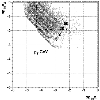
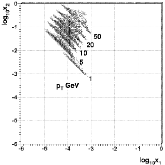
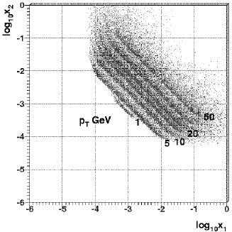
  (a)    (b)   (c)    (d)

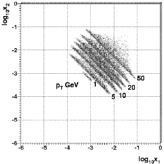
Figure 42: Bjorken $x$ region of LHCb for different values of the $b$ $p_{T}$ for the situation when one of the quarks is in the detector volume (a), both $b$ and $\overline{b}$ are in the detector volume (b). In (c) and (d), analogous distributions are given for ATLAS/CMS.

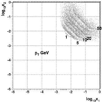
  (a)    (b)

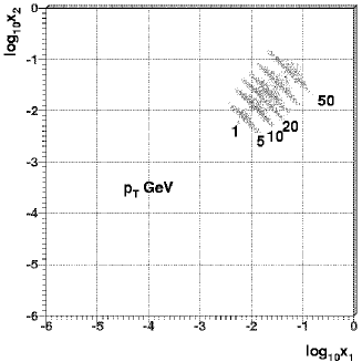
Figure 43: Bjorken $x$ region of CDF for different values of $b$ $p_{T}$ for the situation when one of the quarks is in the detector volume (a), both $b$ and $\overline{b}$ quarks are in the detector volume (b).

7.4 Single $b$ quark production

7.4.1 Theoretical motivations

The inclusive differential cross section $d\sigma/dp_{T}d\eta$, where $p_{T}$ and $\eta$ are the transverse momentum and the pseudorapidity of the $b$ or $\overline{b}$ quarks, provide the basic information on $b$ production. As discussed in the previous section, next-to-leading order (NLO) calculations give a cross section lower than CDF and D0 data by a factor of $\sim 2.4$ [12]. However, the shape of the $p_{T}$ distribution is well reproduced by LO+NLO predictions, by a semihard model of the BFKL type [123] and also by Pythia [124]. In the region of high $p_{T}$, the effects of higher order contributions are taken into account by means of the resummation technique [125] [23] [126]. In ref. [23] LO+NLO contributions are included together with the resummation of all terms of order $\alpha_{s}^{k}\ln^{k}(p_{T}/m_{b})$ and $\alpha_{s}^{k+)}\ln^{k}(p_{T}/m_{b})$. These contributions change the shape of the $p_{T}$ spectrum. Thus measurements of high $p_{T}$ single $b$-spectra may be considered as a dedicated test for the QCD resummation technique.

7.4.2 Measurement possibilities

Experiments can measure the doubly differential cross section $d\sigma/dp_{T}d\eta$, where $p_{T}$ and $\eta$ are the transverse momentum and the pseudorapidity of a $B$ hadron, or of a jet associated with a $B$ hadron, or only one of the decay products of a $B$ hadron (for example $J/\psi$ or $\mu$). From these experimentally measured quantities, the $d\sigma/dp_{T}d\eta$ of the parent $b$-quark can be extracted, using appropriate models of hadronization and decay.

The determination of the absolute value of the cross section is also important. Three independent measurements (ATLAS, CMS and LHCb) can be done at the same energy. The determination of the absolute cross sections is always difficult, since it requires a precise understanding of the luminosity, of the trigger and reconstruction efficiency and of the background contributions. Several techniques of luminosity measurement are under study. It appears that precisions of $\sim 3\%$ could be achieved [127]. The overlap in the detection phase space of ATLAS, CMS and LHCb, in the region $1.8<\eta<2.5$ and $p_{T}>10$ GeV, can be used for cross-checks.

7.4.3 Exclusive channels

From trigger and offline studies and the present experience with CDF it is known that the three LHC experiments can provide high statistics samples of some exclusive $B$-decay channels cleanly separated from the background. The statistically dominant channels are those containing $J/\psi\rightarrow\mu^{+}\mu^{-}$ ($B_{d}\rightarrow J/\psi K^{0}$, $B_{d}\rightarrow J/\psi K^{*}$, $B^{\pm}\rightarrow J/\psi K^{\pm}$ and $B^{0}_{s}\rightarrow J/\psi\phi$), which are also needed for CP violation studies. Moreover, LHCb will cleanly separate large statistics of purely hadronic exclusive decays, where the dominant ones are $B_{d}\rightarrow D^{*-}\pi^{+}$ and $B_{d}\rightarrow D^{*-}a_{1}^{+}$. With these processes one can cover the differential $p_{T}$ cross section measurements starting approximately from $p_{T}>10$ GeV for ATLAS and CMS and $p_{T}>2$ GeV for LHCb respectively. The numbers of these events after three years of run at luminosities of $10^{33}cm^{-2}s^{-1}$ for ATLAS and CMS and five years at $2\cdot 10^{32}cm^{-2}s^{-1}$ for LHCb, are shown in fig. 44 as a function of a minimal transverse momentum of the $B$-hadron $p_{T}$.

7.4.4 Inclusive $b\rightarrow J/\psi X$channels

The inclusive channels $b\rightarrow J/\psi X$ can be used to extend the available statistics for production measurements to high transverse momenta (fig. 44).

A preliminary study from CMS [128] shows that for $p_{T}^{J/\psi}\sim 300$ GeV, which corresponds to $p_{T}^{b}\sim 550$ GeV, a b-tagging efficiency of $\sim 50\%$ can be achieved with a $J/\psi$ mass and decay length reconstruction. This will give a signal-to-noise ratio of $\sim 2.5$ taking into account the prediction for prompt $J/\psi$ production of ref. [93].

In ATLAS a study has been done [129] for events $b\rightarrow J/\psi(\mu\mu)X\$in which the $p_{T}$ of the $b$ quark was chosen larger than 50 GeV. In particular, it was shown that the mass resolution of the $J/\psi$ will not be degraded due to events in which a signal reconstructed in the muon system is wrongly associated to a non-muon track in the inner detector.

 

Figure 44: Number of triggered and reconstructed $B$-hadrons as function of a lower cut on the $B$-hadron transverse momentum $p_{T}$. Figure (a) shows the ATLAS expectations for inclusive and exclusive $B$-hadrons decays to $J/\psi$ after 3 years, with an integrated luminosity of $30\mathrm{f}b^{-1}$. The full line corresponds to inclusive events, the dashed line to the sum of all exclusive channels. Fig. (b) shows the LHCb expectations for exclusive $B$-hadrons decays after 5 years. The solid line is for all statistically dominant channels, the dashed line shows only the channels with a $J/\psi$ in the final state.

7.4.5 Inclusive $b$-jet production

Another method for $b$ production studies discussed at the workshop was based on inclusive $b$-jet reconstruction. In both ATLAS and CMS this technique was developed for the Higgs search [130] [121]. The $b$-jet cross section is expected to be a small fraction (close to or larger than 2% for jets with $E_{T}$ larger than about 20 GeV) of the single-jet cross section [131] [132]. If this method is to be used for single $b$ quark production, it will require prescaling of the trigger for the lower $p_{T}$ region or a cut on very high transverse momenta ($p_{T}>150$ GeV), to reduce the huge rate of non-$b$ QCD background [133].

Figure 45 shows the preliminary results of the CMS $b$-tagging efficiency and mistagging probability for high $E_{T}$ jets using the technique described in  [134]. The study demonstrates that for tagging efficiencies of $35\%-55\%$ the mistagging probability is better than $2\%$ up to $E_{T}\sim 200$ GeV. Beyond that, the $b$-tagging efficiency and mistagging probability deteriorate significantly. The algorithm will be further optimised, possibly including lepton identification.

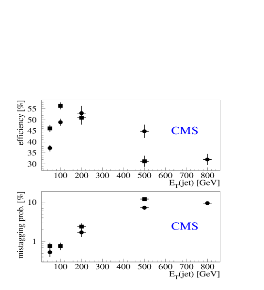
Figure 45: The results of CMS study of $b$-tagging efficiency and mistagging probability as a function of the jet $E_{T}$. The squares represent the results of the phase-1 tracker, the circles those of the phase-2 tracker.

The method of $b$ cross section determination based on inclusive $b$-jet identification will be heavily dependent on the precise understanding of the non $b$-jet rejection factors. Further feasibility studies on this method are necessary.

7.5 Correlations in $b$ production

7.5.1 Theoretical motivations

As discussed in Section 2, the overall normalisation of the production cross section, as well as the normalisation of the inclusive $b$ spectra, remain uncertain within a factor $\sim 2$ because of inherent theoretical uncertainties. Therefore the measurement of these values does not provide a sringent test of NLO contributions. The expected correlations between the $b$ and the $\overline{b}$ quarks can be computed in leading and next-to-leading order [5]. The shapes of two-particle distributions are sensitive to the NLO contribution, and thus can be used for these tests. In particular, distributions in the following quantities involving both the $b$ and $\overline{b}$ quark can be considered: the relative azimuthal distance $\Delta\phi(b\bar{b})<1$, the pair invariant mass, the pair transverse momentum and the pair rapidity.

7.5.2 Measurement possibilities

The choice of the decay channels is driven by the requirement that the acceptance should not vanish when the $b$ and the $\overline{b}$ are close in phase space. The goal is to avoid isolation cuts in both trigger and offline algorithms requiring a large separation between the decay products of the $B$ and of the $\overline{B}$. The processes under consideration are based on the reconstruction of a $J/\psi$ originating from the displaced vertex of a $B$-hadron, and of an additional lepton coming from the semileptonic decay of the associated $\overline{B}$ hadron. For example, in the ATLAS experiment, for an integrated luminosity of $30\;\mathrm{f}b^{-1}$, approximately $\sim 5\cdot 10^{5}$ such events are expected, with the exclusively reconstructed $B$-decays containing the $J/\psi$ (Table 15). CDF and D0 measurements showed that $b\bar{b}$ pairs are mostly produced back-to-back [135]. However the region most sensitive to differences between the models is $\Delta\phi(b\bar{b})<1$ rad, where only $\sim 14\%$ of the events are expected [124]. The statistics may possibly be increased using the semi-inclusive decays $b\overline{b}\rightarrow J/\psi X\$accompanied by a lepton (Table 15). As an example we quote recent studies in ATLAS [129], performed using simulated events with $B_{d}\rightarrow J/\psi K^{0}$, $J/\psi\rightarrow\mu^{+}\mu^{-}$. They indicate that the signal events can indeed be reconstructed in cases when the difference of azimuthal angles between the $J/\psi$ and the other muon is small (Fig. 46). It is important to note that no selection cuts requiring model dependent corrections were necessary.

The study can be extended to events with $J/\psi\rightarrow\mu^{+}\mu^{-}$accompanied by an electron and for $J/\psi\rightarrow e^{+}e^{-}\$ combined with a muon or an electron. Using all these combinations of leptons will allow the measurement of the same variables by different detectors, leading to an improved control of systematic errors.

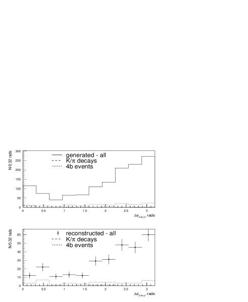
Figure 46: Reconstruction of $\mbox{$b\overline{b}\rightarrow J/\psi(\mu\mu)X\ $}+\mu$ using combined Muon-Inner detector off-line reconstruction in ATLAS.

Table 15: Semi-inclusive and exclusive channels candidates for $b\bar{b}$ studies. Statistics are given for ATLAS after 3 years, with an integrated luminosity of $30\;\mathrm{f}b^{-1}$.

Inclusive channels	Statistics	Exclusive channels	Statistics
		with the same
		lepton content
$\mbox{$b\overline{b}\rightarrow J/\psi(\mu\mu)X\ $}+\mu$	$2.8\cdot 10^{6}$	$b\overline{b}\rightarrow had\mbox{$J/\psi\rightarrow\mu^{+}\mu^{-}$}+\mu$	$2.1\cdot 10^{5}$
$\mbox{$b\overline{b}\rightarrow J/\psi(\mu\mu)X\ $}+e$	$3.6\cdot 10^{6}$	$b\overline{b}\rightarrow had\mbox{$J/\psi\rightarrow\mu^{+}\mu^{-}$}+e$	$2.1\cdot 10^{5}$
$\mbox{$b\overline{b}\rightarrow J/\psi(ee)X\ $}+\mu$	$0.6\cdot 10^{6}$	$b\overline{b}\rightarrow had\mbox{$J/\psi\rightarrow e^{+}e^{-}\ $}+\mu$	$0.9\cdot 10^{5}$

7.6 Multiple heavy quark pair production

7.6.1 Theoretical motivations

At present, only the leading order calculation, $O(\alpha_{s}^{4})$, is available [136] for the $bb\bar{b}\bar{b}$ production cross section. The effects of higher order corrections can only be estimated using the event generator Pythia 5.7. Since the predictions of Pythia  appear to be about a factor of 10 above the leading order analytical calculations [137], further theoretical studies are needed.

7.6.2 Measurement possibilities

Events with four $b$ quarks can be identified in several ways, the most appropriate one depending upon the context. As a background to Higgs search, the requirement is four $b$ jets in the fiducial volume. For the purpose of testing QCD predictions on double $b$ production, it may be sufficient to reconstruct events with three $b$ quarks in the fiducial volume. For three $b$ quarks with $p_{T}>10$ GeV and $|\eta|<2.5$, Pythia gives a cross section of $140$ nb, which corresponds to 140 events produced per second. Despite this large number, it will be necessary to define features allowing on-line selection of these events in the presence of huge non-$b$ and single $b$ backgrounds.

As a source of an incorrect tag in CP violation measurements, the relevant $bb\bar{b}\bar{b}$ events are those with two $b$ hadrons, produced with the same flavour charge, identified in the fiducial volume, while two other $B$-hadrons, produced with the opposite flavour, are not detected. A direct measurement of this case could use reconstructed charged mesons or baryons, which are self-tagging. However the expected statistics of these events is insufficient. In fact, double $b$ production is expected to be only a minor source of wrong tags [138]. Techniques exist to determine the wrong-tag rate from all processes regardless of its origin, which does not need to be identified [138].

Similar to the case of double $b$ production, the production of doubly heavy hadrons, such as the $B_{c}+b+c$, $\Xi_{bc}+b+c$, etc., refers to an $O(\alpha_{s}^{4})$ lowest order QCD process, and also provides a test of perturbative QCD calculations. The question of higher order QCD contributions and, probably, nonperturbative contributions is still open [139]. The total production rate in this case will not be indicative enough to establish the role of different production mechanisms, and the measurement should instead concentrate on the specific event topologies. In particular, various correlations between particles carrying charm and bottom may be of importance.

Measurement possibilities are under investigation for the channel $B_{c}^{(*)}\rightarrow J/\psi\pi$ [140] . A list of possible semileptonic and nonleptonic $B_{c}$ decays can be found for instance in[141]. The decays $B_{c}^{(*)}\rightarrow J/\psi\mu\nu$, $B_{c}^{(*)}\rightarrow J/\psi\rho^{+}$, $B_{c}^{(*)}\rightarrow J/\psi K^{+*}$, $B_{c}^{(*)}\rightarrow J/\psi D_{s}^{+}$ are other potentially interesting modes.

7.7 Other measurements

$B$ hadrons with non-zero spin can be polarized perpendicular to their production plane. Polarization measurements of $b$ hadrons produced in nucleon fragmentation could clarify the problems of different polarization models [142] that failed to reproduce the existing data on strange hyperon production [143]. In particular, information about the quark mass dependence of polarization effects could be obtained. For symmetry reasons, in $pp$ collisions this polarization vanishes at zero rapidity, so that the expected observed polarization in ATLAS and CMS will be smaller than in the more forward LHCb. Using the method of helicity analyses of cascade decay $\Lambda^{0}_{b}\rightarrow\Lambda^{0}J/\psi$ the $\Lambda^{0}_{b}$ polarization can be measured in ATLAS with a precision better than 0.016 [144]. Another approach to $\Lambda^{0}_{b}$ polarisation measurement, using the same decay channel can be found in [145].

In proton-proton collisions a charge production asymmetry of $b$ hadrons is expected. The asymmetry is defined as the difference of production probabilities of a $B$ hadron and its antiparticle. From the theoretical point of view, the asymmetries can provide information on the effects of soft dynamics during the fragmentation and hadronization (i.e., on the soft interactions between the produced $b$ quark and the remnants of the disrupted proton). The relevant physical effects are expected to be unimportant [47] [146] [30] in the central rapidity region covered by ATLAS and CMS. In the more forward region of LHCb the asymmetry may rise to a few percent. A detailed theoretical discussion of this issues are given in Section 5.

Any production asymmetry is always measured in the presence of a CP violation asymmetry originating from $B$-hadron decays. In some cases these two effects are expected to be of the same order. This is the case, for instance, in the channels $B_{d}\rightarrow J/\psi K^{*}(K^{+}\pi^{-})$, $B^{+}\rightarrow J/\psi K^{+}\$ and $\Lambda^{0}_{b}\rightarrow\Lambda^{0}J/\psi$, which are expected to have a small CP violation ($<1\%$). A way of estimating the relative size of these two effects may be based on the fact that the production asymmetry varies with the transverse momentum and the rapidity of produced $b$-quark, while the decay asymmetry should remain the same. Measurements of such small effects will require good understanding of the possible instrumental detection asymmetries.

7.8 Conclusions

The properties of $b$ production at the LHC can be measured by the three experiments, which are complementary in phase space. The small overlap region will allow a cross check on the cross section normalization. The kinematic conditions are such that Bjorken $x$ values sampled in b-production are above 10^-5, a region lower than at the Tevatron, but already covered by HERA. Differential cross section measurements using exclusive $B$ hadron decays will be most important at small $p_{T}$ values. At high $p_{T}$ values and for correlations and multiple heavy flavour production measurements, the statistics can be increased by semi-inclusive $B$ decays containing $J/\psi$. Possible methods using $b$-jets require further study, to control the non-$b$ QCD background. The enormous LHC statistics will also allow to study the production polarization and charge production asymmetries.

8 TUNING OF MULTIPLE INTERACTIONS GENERATED BY PYTHIA

8.1 Introduction

The track multiplicity distribution as well as the transverse momentum distribution of charged particles in proton-proton interactions (the so-called minimum bias events) affect the performances of the low level triggers and the detector occupancy of the LHCb experiment [147]. They should therefore be modelled reliably in Monte Carlo programs. In particular, at LHC energies, multiple interactions play an important role, and should not be neglected.

In Section 8.2 we examine the multiple interaction models available in Pythia [37] to describe the event structure in hadron-hadron collisions. In Section 8.3 we select a compilation of homogeneous data at different energies suitable to tune the multiple interactions parameters of Pythia; the tuning procedure is presented in Section 8.4. We use the phenomenological extrapolations at LHC energy in order to get the predictions for the track multiplicity and the transverse momentum distributions in minimum bias and $b\overline{b}$ events; these are reported in Section 8.5.

8.2 Multiple interaction models

The multiple interactions scenario is needed to describe the multiplicity observables at hadron colliders [148] and is also supported by direct observation [149] [150] [151]. The basic assumption is that several parton-parton interactions can occur within a single hadron-hadron collision. Four different models are available in Pythia. The main parameter of these models, $P_{T_{min}}$, is the minimum transverse momentum of the parton-parton collisions; it effectively controls the average number of parton-parton interactions and hence the average track multiplicity. The differences between the four models, which mainly affect the shape of the multiplicity distribution, are the following:

• Model 1 (default in Pythia)

  All the hadron collisions are equivalent (as opposed to model 3 and 4 below) and all the parton-parton interactions are independent; the $P_{T_{min}}$ parameter represents an abrupt cut-off.

• Model 2

  Same as Model 1 but with a continuous turn-off of the cross section at $P_{T_{min}}$.

• Model 3

  Same as Model 2, but hadronic matter in the colliding hadrons is distributed according to a Gaussian shape, and a varying impact parameter between the two hadrons is assumed.

• Model 4

  Same as Model 3 but the matter distribution is described by two concentric Gaussian distributions.

The varying impact parameter models (Models 3 and 4) were developed [148] to fit the UA5 data [152]. A recent study performed by the CDF collaboration [153] concludes that a varying impact parameter model (Model 3) is also preferred to describe the underlying tracks in $b$ events produced at the Tevatron.

In the absence of published results on multiplicity distributions in minimum bias events at the Tevatron, we compare again the predictions of Model 1 and Model 3 with the UA5 data, using the final charged multiplicity distribution from the full $\overline{p}p$ data sample collected by UA5 at $\sqrt{s}=546$ GeV [154], a recent version of Pythia, and a modern set of parton distribution functions, CTEQ4L [14], tuned on both HERA and Tevatron data. For this comparison, the main multiple interactions parameter ($P_{T_{min}}$) is tuned in each model to reproduce the mean value of the measured charged multiplicity distribution in not single diffractive events ($<N_{ch}>=29.4\pm 0.3\pm 0.9$). We obtain $P_{T_{min}}=1.63\pm 0.02$ for Model 1 and $P_{T_{min}}=1.97\pm 0.03$ for Model 3. The shapes of the multiplicity distributions are compared in fig. 47. It is clear that Model 3 is preferred over Model 1 to describe the UA5 data. In particular the shape of the tail at high multiplicities is reproduced much better by Model 3. The UA5 results are corrected for the lower efficiency expected on double diffractive events. Therefore the simulated samples include the generation of all kind of non single-diffractive events. The uncertainty in the diffractive cross sections relative to the partonic ones can affect the observed discrepancies between the data and the Pythia predictions in the low multiplicity region.

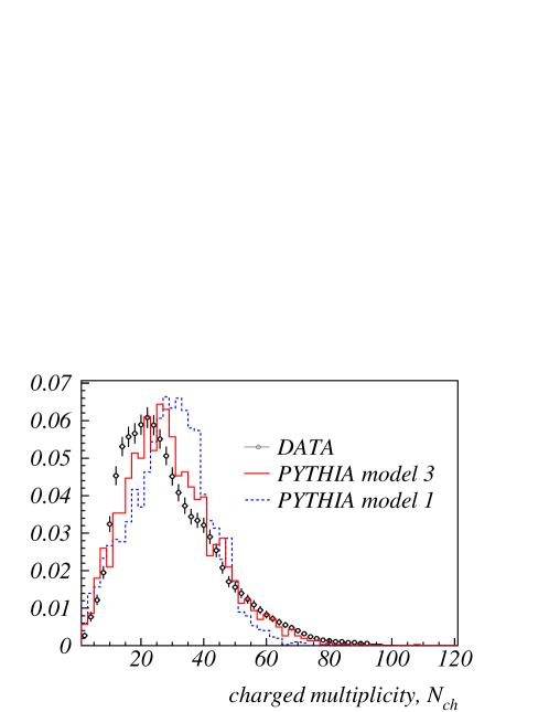
Figure 47: Charged multiplicity distribution for non single-diffractive events in $\overline{p}p$ collisions at $\sqrt{s}=546$ GeV as measured by UA5 [154] compared with Pythia predictions using the CTEQ4L parton distribution functions and either Model 1 (solid) or 3 (dashed) for multiple interactions. In each case the $P_{T_{min}}$ parameter has been tuned to reproduce the mean multiplicity measured in the data.

8.3 Mean charged multiplicity at $\eta=0$

In order to produce realistic Pythia predictions for the multiplicity observables in the LHC environment, it is necessary to take into account the energy dependence of the $P_{T_{min}}$ parameter. Unfortunately there are not many published data concerning the charged multiplicity distribution in minimum bias events at hadron colliders. On the other hand there are some data available relative to the average charged multiplicity in non single-diffractive events, in particular for the central pseudo-rapidity region. Therefore, to study the energy dependence of the $P_{T_{min}}$ parameter at generator level, we consider an homogeneous sample of corrected average charged multiplicity measurements at six different center-of-mass energies ($\sqrt{s}=$ $50$, $200$, $546$, $630$, $900$ and $1800$ GeV) in the pseudo-rapidity region $|\eta|<0.25$ [156] [157]. The energy dependence of $dN_{ch}/d\eta$ at $\eta=0$ is shown in fig. 48a together with the fit of a quadratic function of $\ln(s)$ proposed in Reference [157]; using this fit to extrapolate at LHC energy would predict $dN_{ch}/d\eta=6.11\pm 0.29$ at $\eta=0$.

8.4 Tuning of the multiple interaction parameter $P_{T_{min}}$

The average charged multiplicity measurements performed on non single-diffractive data in $\overline{p}p$ collisions and described in Section 8.3 are used to tune the main multiple interaction parameter in Pythia, $P_{T_{min}}$. We generate non single-diffractive events. At each value of $\sqrt{s}$, the $P_{T_{min}}$ parameter is adjusted to reproduce the average multiplicity measured in the data. The uncertainty on the tuned value of $P_{T_{min}}$ reflects the uncertainty on the data. However, the tuned parameters depend on other aspects of the Pythia simulation: in particular the effects of various choices for the multiple interaction model and the parton distribution functions are investigated. For simplicity, the results of these studies are shown only for some representative settings:

• as an example of pre-HERA parton distribution functions we consider the CTEQ2L [99] set used by default in Pythia versions 5.7, but recently retracted by their authors;

• as an example of post-HERA parton distribution functions we consider the CTEQ4L [14] and GRV94L [158] sets, the latter being the new default in Pythia versions 6.1.

This study is restricted to Models 1 and 3 for multiple interactions (see Section 8.2).

The results of the tuning procedure are shown in fig. 48b: in each case, $P_{T_{min}}$ appears to be monotonically increasing as a function of $\sqrt{s}$. This dependence is much more pronounced for the post-HERA parton distribution functions regardless of the choice for the multiple interactions model.

$\begin{array}[]{cc}\mbox{\includegraphics[width=216.81pt,clip]{ch_new_bw_t.eps}}&\mbox{\includegraphics[width=216.81pt,clip]{fit_all_bw_t.eps}}\end{array}$

Figure 48: a) $dN_{ch}/d\eta$ at $\eta=0$ as a function of $\sqrt{s}$. The solid curve represent a phenomenological fit performed by CDF [157] with the formula ${dN_{ch}}/{d\eta}(s)=(0.023\pm 0.008)\ln^{2}(s)-(0.25\pm 0.19)\ln(s)+(2.5\pm 1.0)$. The two dashed curves represent the 1 sigma variations of the fitted parameters.
b) $\sqrt{s}$-dependence of the $P_{T_{min}}$ parameter for various parton distribution functions and multiple interactions models. The points with error bars are the results of the tuning procedure on the data. The curves are the results of the fits through the points assuming the functional form of Equation 37 and are characterized by the parameters given in Table 16.

It was shown in Reference [159] that the post-HERA parton distribution functions imply an energy-dependent $P_{T}$ cut-off. This is heuristically motivated by the Lipatov-like dependence of the gluonic parton distribution function in the small-$x$ limit:

$$xg(x,Q^{2})\rightarrow{\rm constant}\times x^{-\epsilon}~{}~{}{\rm for}~{}x\rightarrow 0$$ (35)

with $\epsilon\simeq 0.08$, while the pre-HERA parton distribution functions give a reduced charge screening effect and consequently a less sensitive running of the $P_{T}$ cut-off. This is heuristically motivated by the Regge-like dependence of the gluonic parton distribution function in the small-$x$ limit:

$$xg(x,Q^{2})\rightarrow{\rm constant}~{}~{}{\rm for}~{}x\rightarrow 0\;.$$ (36)

In order to extrapolate $P_{T_{min}}$ at LHC energy, one needs to find a reasonable function to fit the tuned $P_{T_{min}}$ values as a function of $\sqrt{s}$ for the different parton distribution functions and multiple interactions models; a four degree of freedom fit is performed using the following exponential form, inspired by the recent implementations added in Pythia since version 6.120 [155]:

$$P_{T_{min}}(\sqrt{s})~{}=~{}P_{T_{min}}^{\rm LHC}\left(\frac{\sqrt{s}}{14~{}{\rm TeV}}\right)^{2\epsilon}\;.$$ (37)

The fitted functions are superimposed on fig. 48b and the results obtained for the fitted parameters $\epsilon$ and $P_{T_{min}}^{\rm LHC}$ are given in Table 16. This quantitative analysis demonstrates that the power law expressed in Equation 37 holds for values of $\epsilon$ between $\simeq 0.08$ and $\simeq 0.10$ if post-HERA parton distribution functions are used, and for somewhat smaller values of $\epsilon$ ($\simeq 0.05$) for the pre-HERA parton distribution functions.

Table 16: Results of the fits describing the exponential running of the Pythia multiple interactions parameter $P_{T_{min}}$ for different parton distribution functions and multiple interactions models.

Mult. int. model	PDF	$P_{T_{min}}^{\rm LHC}$ (GeV/c)	$\epsilon$
3	CTEQ2L	$1.99\pm 0.11$	$0.048\pm 0.006$
3	GRV94L	$4.06\pm 0.24$	$0.103\pm 0.006$
3	CTEQ4L	$3.47\pm 0.17$	$0.087\pm 0.005$
1	CTEQ4L	$3.12\pm 0.16$	$0.100\pm 0.005$

8.5 Pythia predictions at LHC energy

Figures 49a and b show multiplicity and pseudorapidity distributions for charged particles predicted by Pythia at LHC with CTEQ4L and Model 3 for multiple interactions. The value of $P_{T_{min}}$ at LHC is obtained by an extrapolation

$$P_{T_{min}}^{\rm LHC}~{}=~{}P_{T_{min}}^{\rm Tevatron}\left(\frac{14~{}{\rm TeV}}{1.8~{}{\rm TeV}}\right)^{2\epsilon}$$ (38)

where $P_{T_{min}}^{\rm Tevatron}$ is the $P_{T_{min}}$ value tuned at the Tevatron energy of $1.8~{}{\rm TeV}$. For the parameter $\epsilon$, we adopt the results given in Table 16. It is important to note that the predictions $dN_{ch}/d\eta=6.30\pm 0.42$ (for $\epsilon=0.087\mp 0.005$) at $\eta=0$ are consistent with the phenomenological fit displayed in fig. 48a ($dN_{ch}/d\eta=6.11\pm 0.29$).

In order to demonstrate the importance of the correct $P_{T_{min}}$ extrapolation, figs. 49a and b also show results obtained by assuming $P_{T_{min}}^{\rm LHC}=P_{T_{min}}^{\rm Tevatron}$, i.e. $\epsilon=0$ not supported by the data as demonstrated in Section 8.4. The multiplicity distribution has a tail at high multiplicities and $dN_{ch}/d\eta$ at $\eta=0$ is not consistent with that obtained from the phenomenological fit.

$\begin{array}[]{cc}\mbox{\includegraphics[width=216.81pt,clip]{lhc_cteq4l_model3_1.eps}}&\mbox{\includegraphics[width=216.81pt,clip]{lhc_cteq4l_model3_2.eps}}\end{array}$

Figure 49: Pythia predictions at LHC energy, using the CTEQ4L parton distribution functions and Model 3 for multiple interactions with $P_{T_{min}}$ given by Equation 38: the solid and dashed distributions correspond to the central value and $\pm 1\,\sigma$ uncertainties of the fitted value $\epsilon=0.087\pm 0.005$. The dotted histogram is obtained with $\epsilon=0$, i.e. using the $P_{T_{min}}$ value tuned on Tevatron data and ignoring its energy dependence. a) Charged track multiplicity in the entire $4\pi$ solid angle. b) Average charged track multiplicity per unit pseudorapidity, as a function of pseudorapidity.

Figure 50 shows the same distributions as fig. 49, but for the CTEQ2L parton distribution functions. It is interesting to note that, once the extrapolation of $P_{T_{min}}$ is properly done, there is no large difference between the multiplicity and pseudorapidity distributions obtained with different structure functions.

$\begin{array}[]{cc}\mbox{\includegraphics[width=216.81pt,clip]{lhc_cteq2l_model3_1.eps}}&\mbox{\includegraphics[width=216.81pt,clip]{lhc_cteq2l_model3_2.eps}}\end{array}$

Figure 50: Pythia predictions at LHC energy, using the CTEQ2L parton distribution functions and Model  3 for multiple interactions with $P_{T_{min}}$ given by Equation 38: the solid and dashed distributions correspond to the central value and $\pm 1\,\sigma$ uncertainties of the fitted value $\epsilon=0.048\pm 0.006$. The dotted histogram is obtained with $\epsilon=0$, i.e. using the $P_{T_{min}}$ value tuned on Tevatron data and ignoring its energy dependence. a) Charged track multiplicity in the entire $4\pi$ solid angle. b) Average charged track multiplicity per unit pseudorapidity, as a function of pseudorapidity.

Figure 51a-d compare the Pythia predictions for the multiplicity and transverse momentum distributions in the LHCb angular acceptance ($1.8<\eta<4.9$) between minimum bias and $b\overline{b}$ events. These predictions are obtained with CTEQ4L, multiple interactions Model 3 and the proper $P_{T_{min}}$ extrapolation. They show clear differences between minimum bias and $b\overline{b}$ events, in particular higher average multiplicity and transverse momentum for $b\overline{b}$ events.

$\begin{array}[]{cc}\mbox{\includegraphics[width=216.81pt,clip]{cteq4l_model3_1.eps}}&\mbox{\includegraphics[width=216.81pt,clip]{cteq4l_model3_4.eps}}\\ \mbox{\includegraphics[width=216.81pt,clip]{cteq4l_model3_6.eps}}&\mbox{\includegraphics[width=216.81pt,clip]{cteq4l_model3_7.eps}}\\ \end{array}$

Figure 51: Pythia predictions for charged tracks in the LHCb acceptance using the CTEQ4L parton distribution functions and Model 3 for multiple interactions with proper $P_{T_{min}}$; the normalized predictions for $b\overline{b}$ events (dashed curve) and minimum bias events (solid curve) are superimposed. a) Charged track multiplicity distribution. b) Transverse momentum distribution of charged tracks. c) Distribution of the maximum transverse momentum of charged tracks. d) Rejection efficiency as a function of a traverse momentum cut (an event is rejected if all the charged tracks have a transverse momentum below the cut).

$\begin{array}[]{cc}\mbox{\includegraphics[width=216.81pt,clip]{cteq4l_model1_1.eps}}&\mbox{\includegraphics[width=216.81pt,clip]{cteq4l_model1_4.eps}}\end{array}$

Figure 52: Pythia predictions for charged tracks in the LHCb acceptance using the CTEQ4L parton distribution functions and Model 1 for multiple interactions with proper $P_{T_{min}}$; the normalized predictions for $b\overline{b}$ events (dashed curve) and minimum bias events (solid curve) are superimposed. a) Charged track multiplicity distribution. b) Transverse momentum distribution of charged tracks.

Pythia predictions with multiple interactions Model 1 for the multiplicity and transverse momentum distributions are shown in fig. 52 for minimum bias and $b\overline{b}$ events. Compared to the results obtained with Model 3, less significant differences between minimum bias and $b\overline{b}$ events is observed. In Section 8.2 we have stressed that a varying impact parameter model for multiple interactions (i.e. Model 3) is needed to describe the charged track multiplicity in hadron-hadron interactions. There are arguments in favour of adopting a multiple interactions model with varying impact parameter to describe the heavy flavour production at hadron colliders [160], though there are no experimental data at low transverse momentum and high pseudorapidity (i.e. in the LHCb acceptance region). A more detailed discussion on the effect of multiparton interactions in $b\overline{b}$ events at LHCb can be found in Reference [161].

8.6 Conclusions

Comparisons between Pythia and experimental data demonstrate that, in order to reproduce the charged track multiplicity spectrum, a varying impact parameter model has to be adopted.

The varying impact parameter models predict sensitive differences in multiplicity and $P_{T}$ distribution between light and heavy flavour events.

The running of the $P_{T}$ cut-off parameter in Pythia multiple interactions is mandatory. Predictions made at LHC energy with a fixed $P_{T}$ cut-off tuned at lower energies overestimate the multiplicity observables. Taking into account the running of the $P_{T}$ parameter is even more important if post-HERA parton distribution functions are used.

References

- [1] P. Nason, S. Dawson and R. K. Ellis, Nucl. Phys. B303, 607 (1988) .
- [2] W. Beenakker, H. Kuijf, W.L. van Neerven and J. Smith, Phys. Rev. D40198954.
- [3] P. Nason, S. Dawson and R. K. Ellis, Nucl. Phys. B327, 49 (1989) ; erratum ibid. B335, 260 (1990).
- [4] W. Beenakker, W.L. van Neerven, R. Meng, G.A. Schuler and J. Smith, Nucl. Phys. B351, 507 (1991) .
- [5] M. Mangano, P. Nason and G. Ridolfi, Nucl. Phys. B373, 295 (1992) .
- [6] R. K. Ellis and P. Nason, Nucl. Phys. B312, 551 (1989) .
- [7] J. Smith and W.L. van Neerven, Nucl. Phys. B374, 36 (1992) .
- [8] S. Frixione, M.L. Mangano, P. Nason and G. Ridolfi, Nucl. Phys. B412, 225 (1994) .
- [9] E. Laenen, S. Riemersma, J. Smith and W.L. van Neerven, Nucl. Phys. B392, 162 (1993) .
- [10] E. Laenen, S. Riemersma, J. Smith and W.L. van Neerven, Nucl. Phys. B392, 229 (1993) .
- [11] B.W. Harris and J. Smith, Nucl. Phys. B452, 109 (1995) , hep-ph/9503484.
- [12] S. Frixione, M.L. Mangano, P. Nason and G. Ridolfi, “Heavy-Quark Production”, hep-ph/9702287, published in “Heavy Flavours II”, eds. A.J. Buras and M. Lindner, Advanced Series on Directions in High Energy Physics, (World Scientific Publishing Co., Singapore).
- [13] A.D. Martin, R.G. Roberts, W.J. Stirling and R.S. Thorne, Eur. Phys. J. C4, 463 (1998), hep-ph/9803445.
- [14] H.L. Lai et al., CTEQ Collaboration, Phys. Rev. D5519971280, hep-ph/9606399.
- [15] M. Beneke, Proceedings of “Heavy Flavour 8”, Southampton, UK, 1999, hep-ph/9911490.
- [16] K.G. Chetyrkin and M. Steinhauser, DESY-99-174, hep-ph/9911434.
- [17] K. Melnikov and T. van Ritbergen, SLAC-PUB-8321, hep-ph/9912391.
- [18] R. Bonciani, S. Catani, M. Mangano and P. Nason, Nucl. Phys. B529, 424 (1998) , hep-ph/9801375.
- [19] R.K. Ellis and D.A. Ross, Nucl. Phys. B345, 79 (1990) .
- [20] J. C. Collins and R. K. Ellis, Nucl. Phys. B360, 3 (1991) .
- [21] S. Catani, M. Ciafaloni and F. Hautmann, Phys. Lett. B242, 97 (1990).
- [22] S. Catani, M. Ciafaloni and F. Hautmann, Nucl. Phys. B366, 135 (1991) .
- [23] M. Cacciari, M. Greco and P. Nason, JHEP05(1998)007, hep-ph/9803400.
-
[24]
B. Mele and P. Nason, Phys. Lett. B245, 635 (90);
B. Mele and P. Nason, Nucl. Phys. B361, 626 (91) . - [25] L. Apanasevich et al., Phys. Rev. D591999074007, hep-ph/9808467.
-
[26]
G. Altarelli, N. Cabibbo, G. Corbò and L. Maiani, Nucl. Phys. B208, 365 (82) ;
N. Cabibbo, G. Corbò and L. Maiani, Nucl. Phys. B155, 93 (79) . - [27] K. Abe et al., SLD Collaboration, Contributed paper to the International Europhysics Conference on High-Energy Physics (EPS-HEP 99), Tampere, Finland, Jul. 1999, and 19th International Symposium on Lepton and Photon Interactions at High-Energies (LP 99), Stanford, CA, Aug. 1999, SLAC-PUB-8153, hep-ex/9908032.
- [28] G. Marchesini and B. R. Webber, Nucl. Phys. B310, 461 (1988); G. Marchesini, B. R. Webber, G. Abbiendi, I. G. Knowles, M. H. Seymour and L. Stanco, HERWIG 5.1, Comput. Phys. Commun. 67, 465 (1992); G. Corcella et al., HERWIG 6.1, hep-ph/9912396. For this study the public version 5.8 of HERWIG was used. We checked that the results discussed here have not changed with higher versions. Version features and various parameter tunings can be found from: http://hepwww.rl.ac.uk/theory/seymour/herwig/.
- [29] G. Wrochna, CMS-CR-1996-002.
- [30] WA82 Collaboration, M. Adamovich et al., Phys. Lett. B305 (1993) 402; E769 Collaboration, G.A. Alves et al., Phys. Rev. Lett. 72 (1994) 812; E791 Collaboration, E.M. Aitala et al., Phys. Lett. B371 (1996) 157.
- [31] E. Norrbin, Proceedings of the International Europhysics Conference on High-Energy Physics (EPS-HEP 99), Tampere, Finland, 15-21 July 1999, LU-TP-99-28, hep-ph/9909437.
- [32] E. Norrbin and T. Sjöstrand, Phys. Lett. B442 (1998) 407, in preparation.
- [33] S.J. Brodsky, P. Hoyer, C. Peterson and N. Sakai, Phys. Lett. B93 (1980) 451; S.J. Brodsky, C. Peterson and N. Sakai, Phys. Rev. D23 (1981) 2745.
- [34] B. Andersson, G. Gustafson, G. Ingelman and T. Sjöstrand, Phys. Rep. 97 (1983) 31.
- [35] R. Vogt and S.J. Brodsky, Nucl. Phys. B438 (1995) 261.
- [36] S.J. Brodsky, P. Hoyer, A.H. Mueller and W.-K. Tang, Nucl. Phys. B369 (1992) 519.
- [37]
- [38] T. Sjöstrand, Phys. Lett. B157 (1985) 321.
- [39] E.D. Bloom and F.J. Gilman, Phys. Rev. D4 (1971) 2901; J.J. Sakurai, Phys. Lett. 46B (1973) 207; H. Fritzsch, Phys. Lett. 67B (1977) 217; R.A. Bertlmann, G. Launer and E. de Rafael, Nucl. Phys. B250 (1985) 61 and references therein.
- [40] E. Braaten, S. Narison and A. Pich, Nucl. Phys. B373 (1992) 581.
- [41] R. Vogt, S.J. Brodsky and P. Hoyer, Nucl. Phys. B360, 67 (1991).
- [42] R. Vogt, S.J. Brodsky and P. Hoyer, Nucl. Phys. B383, 643 (1992).
- [43] R. Vogt, LBNL-43095, in the proceedings of the LHC Working Group on Production, P. Nason and G. Ridolfi covenors, CERN, 4/99. The proceedings are available on the web at http://home.cern.ch/n/nason/www/lhc99/15-04-99/.
- [44] T. Gutierrez and R. Vogt, Nucl. Phys. B539 (1999) 189.
- [45] J.J. Aubert et al. (EMC Collab.), Phys. Lett. 110B, 73 (1982); E. Hoffmann and R. Moore, Z. Phys. C20, 71 (1983); B.W. Harris, J. Smith, and R. Vogt, Nucl. Phys. B461, 181 (1996).
- [46] R. Vogt and S.J. Brodsky, Nucl. Phys. B438 261 (1995).
- [47] R. Vogt and S.J. Brodsky, Nucl. Phys. B478, 311 (1996).
- [48] R. Vogt and S.J. Brodsky, Phys. Lett. B349, 569 (1995).
- [49] J. Badier et al. (NA3 Collab.), Phys. Lett. 114B, 457 (1982); 158B, 85 (1985).
- [50] R. Vogt, Nucl. Phys. B446, 159 (1995).
- [51] E. L. Berger and D. Jones, Phys. Rev. D23, 1521 (1981).
- [52] R. Baier and R. Rückl, Phys. Lett. B102, 364 (1981).
- [53] G. T. Bodwin, E. Braaten and G. P. Lepage, Phys. Rev. D51, 1125 (1995) hep-ph/9407339; erratum ibid. D55, 5853 (1997).
- [54] H. Fritzsch, Phys. Lett. 67B, 217 (1977).
- [55] F. Halzen, Phys. Lett. 69B, 105 (1977).
- [56] M. Gluck, J. F. Owens and E. Reya, Phys. Rev. D17, 2324 (1978).
- [57] R. Gavai, D. Kharzeev, H. Satz, G. A. Schuler, K. Sridhar and R. Vogt, Int. J. Mod. Phys. A10, 3043 (1995), hep-ph/9502270.
- [58] G. A. Schuler and R. Vogt, Phys. Lett. B387, 181 (1996), hep-ph/9606410.
- [59] J. F. Amundson, O. J. Eboli, E. M. Gregores and F. Halzen, Phys. Lett. B390, 323 (1997), hep-ph/9605295.
- [60] A. Edin, G. Ingelman and J. Rathsman, Phys. Rev. D56, 7317 (1997), hep-ph/9705311.
- [61] S.J. Brodsky, Int. J. Mod. Phys. A12, 4087 (1997), hep-ph/9609415.
- [62] P. Hoyer and S. Peigne, Phys. Rev. D59, 034011 (1999), hep-ph/9806424.
- [63] P. Hoyer, Nucl. Phys. Proc. Suppl. 75B, 153 (1999), hep-ph/9809362.
- [64] E. Braaten, S. Fleming and T. C. Yuan, Ann. Rev. Nucl. Part. Sci. 46 (1996) 197 hep-ph/9602374.
- [65] M. Beneke, hep-ph/9703429.
- [66] M. Krämer, hep-ph/9707449.
- [67] G. P. Lepage, L. Magnea, C. Nakhleh, U. Magnea and K. Hornbostel, Phys. Rev. D46 (1992) 4052, hep-lat/9205007.
- [68] G. T. Bodwin, E. Braaten and G. P. Lepage, Phys. Rev. D46, 1914 (1992), hep-lat/9205006.
- [69] F. Abe et al., CDF Collaboration, Phys. Rev. Lett. 69, 3704 (1992).
- [70] F. Abe et al.,CDF Collaboration, Phys. Rev. Lett. 79, 572 (1997).
- [71] R. Baier and R. Rückl, Z. Phys. C19, 251 (1983).
- [72] R. Gastmans, W. Troost and T. T. Wu, Nucl. Phys. B291, 731 (1987).
- [73] E. Braaten and T. C. Yuan, Phys. Rev. Lett. 71, 1673 (1993), hep-ph/9303205.
- [74] M. Cacciari and M. Greco, Phys. Rev. Lett. 73, 1586 (1994), hep-ph/9405241.
- [75] E. Braaten, M. A. Doncheski, S. Fleming and M.L. Mangano, Phys. Lett. B333, 548 (1994), hep-ph/9405407.
- [76] D. P. Roy and K. Sridhar, Phys. Lett. B339, 141 (1994), hep-ph/9406386.
- [77] E. Braaten and S. Fleming, Phys. Rev. Lett. 74, 3327 (1995), hep-ph/9411365.
- [78] M. Cacciari, M. Greco, M.L. Mangano and A. Petrelli, Phys. Lett. B356, 553 (1995), hep-ph/9505379.
- [79] P. Cho and A. K. Leibovich, Phys. Rev. D53, 150 (1996), hep-ph/9505329.
- [80] P. Cho and A. K. Leibovich, Phys. Rev. D53, 6203 (1996), hep-ph/9511315.
- [81] H.L. Lai et al., CTEQ Collaboration, Eur. Phys. J. C12, 375 (2000), hep-ph/9903282.
- [82] W. Buchmüller and S. H. Tye, Phys. Rev. D24, 132 (1981).
- [83] E. J. Eichten and C. Quigg, Phys. Rev. D52, 1726 (1995), hep-ph/9503356.
- [84] M. Beneke and M. Krämer, Phys. Rev. D55, 5269 (1997), hep-ph/9611218.
- [85] M. Beneke, I. Z. Rothstein and M. B. Wise, Phys. Lett. B408, 373 (1997), hep-ph/9705286.
- [86] J. H. Kühn and E. Mirkes, Phys. Rev. D48, 179 (1993), hep-ph/9301204.
- [87] A. Petrelli, M. Cacciari, M. Greco, F. Maltoni and M.L. Mangano, Nucl. Phys. B514, 245 (1998), hep-ph/9707223.
- [88] A. Petrelli, hep-ph/9910274.
- [89] M. Krämer, Nucl. Phys. B459, 3 (1996), hep-ph/9508409.
- [90] J. C. Collins, D. E. Soper and G. Sterman, Nucl. Phys. B250, 199 (1985).
- [91] M. Cacciari, hep-ph/9910412.
- [92] K. Sridhar, A. D. Martin and W. J. Stirling, Phys. Lett. B438, 211 (1998), hep-ph/9806253.
- [93] B. Cano-Coloma and M. A. Sanchis-Lozano, Nucl. Phys. B508, 753 (1997), hep-ph/9706270.
- [94] M.A. Sanchis-Lozano, hep-ph/9907497.
- [95] B. A. Kniehl and G. Kramer, Eur. Phys. J. C6, 493 (1999), hep-ph/9803256.
- [96] M. Cacciari and M. Krämer, Phys. Rev. Lett. 76, 4128 (1996), hep-ph/9601276.
- [97] P. Ko, J. Lee and H. S. Song, Phys. Rev. D54, 4312 (1996), hep-ph/9602223; Erratum: ibid. D60, 119902 (1999).
- [98] M. Beneke, F. Maltoni and I. Z. Rothstein, Phys. Rev. D59, 054003 (1999), hep-ph/9808360.
- [99] W. K. Tung, Prepared for International Workshop on Deep Inelastic Scattering and Related Subjects, Eilat, Israel, 6-11 Feb 1994.
- [100] P. Cho and M. B. Wise, Phys. Lett. B346, 129 (1995), hep-ph/9411303.
- [101] M. Beneke and I. Z. Rothstein, Phys. Lett. B372, 157 (1996), hep-ph/9509375; erratum ibid. D54, 7082 (1997).
- [102] A. K. Leibovich, Phys. Rev. D56, 4412 (1997), hep-ph/9610381.
- [103] CDF collaboration, CDF Note 4876, unpublished.
- [104] CDF collaboration, CDF Note 5029, unpublished.
- [105] E. Braaten, B. A. Kniehl and J. Lee, hep-ph/9911436.
- [106] F. Abe et al., CDF Collaboration, Phys. Rev. Lett. 75, 4358 (1995).
- [107] T. Affolder et al., CDF Collaboration, hep-ex/9910025.
- [108] CDF collaboration, CDF Note 5027, unpublished;
- [109] M.L. Mangano, hep-ph/9507353.
- [110] J. L. Domenech and M. A. Sanchis-Lozano, hep-ph/9911332.
- [111] C. S. Kim, J. Lee and H. S. Song, Phys. Rev. D55 (1997) 5429 hep-ph/9610294.
- [112] P. Mathews, K. Sridhar and R. Basu, Phys. Rev. D60 (1999) 014009 hep-ph/9901276.
- [113] E. Braaten, J. Lee and S. Fleming, Phys. Rev. D60 (1999) 091501 hep-ph/9812505.
- [114] P. Mathews, P. Poulose and K. Sridhar, Phys. Lett. B438 (1998) 336 hep-ph/9803424.
- [115] K. Sridhar, Phys. Rev. Lett. 77 (1996) 4880 hep-ph/9609285.
- [116] E. Richter-Was and M. Sapinski, Acta Phys.Polon, B30, 1001 (1999).
-
[117]
I. Efthymiopoulos for the ATLAS collaboration,
Acta Phys.Polon.B30,2309 (1999);
The ATLAS Collaboration, CERN/LHCC/97-16 (1997);
The ATLAS Collaboration, CERN/LHCC/97-17 (1997);
The ATLAS Collaboration, CERN/LHCC/98-14 (1998);
The ATLAS Collaboration, CERN/LHCC/96-42 (1996);
The CMS Collaboration, CERN/LHCC/94-38 (1994);
O. Schneider, Proceedings of Beauty ’99, to be published in NIM (1999);
LHCb Collaboration, CERN/LHCC/98-4 (1998). -
[118]
The ATLAS collaboration, CERN/LHCC/98-14 (1998), chapter 14,
pp. 367-402;
The ATLAS collaboration, CERN/LHCC/98-15 (1998), chapter 8, pp. 127-134. - [119] G. Wrochna, Proceedings of the Second Workshop on Electronics for LHC Experiments, LHCC , 293 (1996).
-
[120]
The ATLAS collaboration, CERN/LHCC/98-15 (1998), chapter 10,
pp. 209-234;
The ATLAS collaboration, CERN/LHCC/97-16 (1997), chapter 5, pp. 121-143. - [121] The CMS Collaboration, CERN/LHCC/94-38 (1994).
- [122] S. Riess for the H1 and Zeus collaborations, Proceedings of the International Conference on Hadron Structure (HS 98),(1998).
-
[123]
E.A. Kuraev, L.N. Lipatov and V. Fadin,
Sov. Phys. JETP 44, 443 (1976) , Sov. Phys. JETP 45, 199 (1977) ;
Y.Y. Balitzkij and L.N. Lipatov, Sov. J. Nucl. Phys. 28, 822 (1978). - [124] S.P. Baranov and M. Smižanská, ATLAS Internal Note ATL-PHYS-98-133 (1998);
- [125] M. Cacciari and M. Greco, Nucl. Phys. B421, 1994 (530) .
- [126] F.I. Olness, R.J. Scalise and Wu-Ki Tung, Phys. Rev. D590145061999.
- [127] K. Piotrzkowski, ATLAS Internal Note ATL-PHYS-96-077 (1998).
- [128] V. Drollinger and N. Stepanov, CMS NOTE in preparation (2000).
- [129] S.Robins, ATLAS Internal Note ATL-COM-PHYS-2000-006 (2000).
- [130] ATLAS collaboration, CERN/LHCC/99-14 (1999), chapter 10, pp. 317-346.
- [131] The ATLAS collaboration, CERN/LHCC/98-15 (1998), chapter 2, pp. 3-13.
- [132] M.L. Mangano and S. Frixione, Nucl. Phys. B483, 321 (1997) .
- [133] J. Baines et al, ATLAS Internal Note ATL-DAQ-98-121 (1998).
- [134] V. Drollinger and N. Stepanov, CMS NOTE in preparation (2000).
-
[135]
F. Abe et al., CDF Collaboration, Phys. Rev. D5319961051.
S. Abachi et al., D0 Collaboration, Phys. Lett. B370, 239 (1996). - [136] A.K. Likhoded, A.V.Berezhnoy, private communication.
- [137] S.P. Baranov, private communication.
- [138] ATLAS collaboration, CERN/LHCC/99-15 (1999), chapter 17, pp. 561-616.
-
[139]
A.V. Berezhnoy, V.V. Kiselev, and A.K. Likhoded, Sov. J. Nucl. Phys. 59, 909 (1996);
S.P. Baranov, Phys. Rev. D5419963228. - [140] F. Albiol et al., ATLAS Internal Note ATL-PHYS-94-058(1994).
- [141] You-Shan Dai and Dong-Sheng Du, Eur. Phys. J. C9, 557 (1999).
-
[142]
T.A. De Grand and H.I.Miettinen, Phys. Rev. D24, 2419 (1981);
Y. Hama and T. Kodama, Phys. Rev. D48, 3116 (1993);
J. Ellis, D. Kharzeev and A. Kotzinian, Z. Phys. C69, 467 (1996);
W.G.D. Dharmaratna and G.R. Goldstein, Phys. Rev D53, 1073 (1996). - [143] J. Lach, FERMILAB-CONF-92-378 (1992).
- [144] J. Hrivnac, R. Lednicky and M. Smizanska, J. Phys. G21, 629 (1995).
- [145] A. Fridman, R. Kinnunen and N. Neumeister, HEPHY PUB 609-94 LPNHE 94-07 (1994).
- [146] R.C. Hwa, Phys. Rev. D51, 85 (1995).
- [147] S. Amato et al., LHCb Collaboration, CERN/LHCC 98-4.
- [148] T. Sjöstrand and M. van Zijl, Phys. Rev. D36, 2019 (1987).
- [149] T. Akesson et al., AFS Collaboration, Z. Phys. C 34, 163 (1987).
- [150] J. Alitti et al., UA2 Collaboration, Phys. Lett. B268, 145 (1991).
- [151] F. Abe et al., CDF Collaboration, Phys. Rev. D47, 4857 (1993).
- [152] G.J. Alner et al., UA5 Collaboration, Phys. Lett. B138, 304 (1983).
- [153] F. Abe et al., CDF Collaboration, Phys. Rev. D59, 32001 (1999).
- [154] G.J. Alner et al., UA5 Collaboration, Phys. Reports 154, 247 (1987).
- [155] T. Sjöstrand, http://www.thep.lu.se/~torbjorn/Pythia.html.
- [156] G.J. Alner et al., UA5 Collaboration, Z. Phys. C 33, 1 (1986).
- [157] F. Abe et al., CDF Collaboration, Phys. Rev. D41, 2330 (1989).
- [158] M. Gluck et al., Z. Phys. C 67, 433 (1995).
- [159] T. Sjöstrand, In “QCD and Weak Boson Physics”, Proceedings, Workshop, Fermilab, USA, March 4-6, 1999, to be published.
- [160] F. Abe et al., CDF Collaboration, Phys. Rev. Lett. 75, 1451 (1995).
- [161] P. Galumian, LHCb public note EXPT 97-019 (1997).