Timelike and spacelike QCD characteristics of the $e^{+}e^{-}$ annihilation process

Abstract

We consider the Adler $D$-function, which is defined in the spacelike region, and the $e^{+}e^{-}$annihilation ratio smeared, according to the Poggio, Quinn, and Weinberg method, which is determined for timelike argument. We show that the method of the nonperturbative $a$-expansion allows one to describe these Euclidean and Minkowskian characteristics of the process of $e^{+}e^{-}$ annihilation down to the lowest energy scales.

1. In quantum chromodynamics, it is important to determine the “simplest” objects which allow one to check direct consequences of the theory without using model assumptions in an essential manner. Comparison of theoretical results for these objects with experimental data allows us to justify transparently the validity of basic statements of the theory, and make some conclusions about completeness and efficiency of the theoretical methods used. Some single-argument functions which have a straightforward connection with experimentally measured quantities can play the role of these objects. A theoretical description of inclusive processes can be expressed in terms of functions of this sort. Let us mention among them moments ${\rm{M}}_{n}(Q^{2})$ of the structure functions in inelastic lepton-hadron scattering and the hadronic correlator $\Pi(s)$ (or the corresponding Adler $D$-function), which appear in the processes of $e^{+}e^{-}$ annihilation into hadrons or the inclusive decay of the $\tau$ lepton.

In this paper we consider such objects for the process of $e^{+}e^{-}$ annihilation into hadrons. Here, the point is that the experimentally measured ratio of hadronic and leptonic cross-sections, $R_{e^{+}e^{-}}(s)$, is not suitable at the present stage of development of the theory to provide a description independent of model considerations. However, it is possible to construct simpler objects than the $R_{e^{+}e^{-}}$-ratio. These are the Adler function $D(Q^{2})$ [1], which is defined in the Euclidean region, and the quantity $R_{\Delta}(s)$ constructed by the Poggio, Quinn, and Weinberg “smearing” method [2] and defined in the Minkowskian region.

The theoretical method, which we will use here, is the nonperturbative expansion technique suggested in Refs. [3]. This approach is based on the idea of variational perturbation theory (VPT) [4], which in the case of QCD leads to a new small expansion parameter. To compare the results with experiment we will use the new “experimental data” for the Adler function that has been recently obtained in Ref. [5] and the smeared “experimental curve” corresponding to the $R$-ratio taken from Refs. [6, 7].

2. We use the method of constructing the so-called floating or variational series in quantum theory. Within this approach, a certain variational procedure is combined with the possibility of calculating corrections to the principal contribution which allows the possibility of probing the validity of the leading contribution and the region of applicability of the results obtained. At present, this idea finds many applications in the development of various approaches, which should enable us to go beyond perturbation theory. Among these are the Gaussian effective potential method [8], the optimized $\delta$-expansion [9], and the VPT approach [4].

We will apply a nonperturbative QCD expansion based on a new small expansion parameter [3]. Within this method, a quantity under consideration can be represented in the form of a series, which is different from the conventional perturbative expansion and can be used to go beyond the weak-coupling regime. This allows one to deal with considerably lower energies than in the case of perturbation theory.

The new expansion parameter $a$ is connected with the initial coupling constant $g$ by the relation

$$\lambda\,=\,\frac{g^{2}}{{(4\pi)}^{2}}\,=\,\frac{\alpha_{s}}{4\pi}\,=\,\frac{1}{C}\,\frac{a^{2}}{{(1-a)}^{3}}\,,$$ (1)

where $C$ is a positive constant. As follows from (1), for any value of the coupling constant $g$, the expansion parameter $a$ obeys the inequality

$$0\leq a<1\,.$$ (2)

While remaining within the range of applicability of the $a$-expansion, one can deal with low-energy processes where $g$ is no longer small.

The positive parameter $C$ plays the role of an auxiliary parameter of a variational type, which is associated with the use of a floating series. The original quantity, which is approximated by this expansion, does not depend on the parameter $C$; however, any finite approximation depends on it due to the truncation of the series. Here we will fix this parameter using some further information, coming from the potential approach to meson spectroscopy. In the framework of this approach consider the following approximations to the renormalization group $\beta$-function, the functions ${\beta}^{(3)}$ and ${\beta}^{(5)}$, which are obtained if one takes into consideration the terms $O(a^{3})$ and $O(a^{5})$ in the corresponding renormalization constant $Z_{\lambda}$. As has been shown in Ref. [3], $C$ is determined by requiring that $-{\beta}^{(k)}(\lambda)/\lambda$ tends to 1 for sufficiently large $\lambda$, which gives $C_{3}=4.1$ and $C_{5}=21.5$. The increase of $C_{k}$ with the order of the expansion is explained by the necessity to compensate for the higher order contributions. A similar phenomenon takes place also in zero- and one-dimensional models. The behavior of the functions $-\,{\beta}^{(k)}(\lambda)/{\lambda}$ gives evidence for the convergence of the results, in accordance with the phenomenon of induced convergence. The behavior of the $\beta$-function at large value of the coupling constant, $-{\beta}^{(k)}(\lambda)/{\lambda}\simeq 1$, corresponds to the infrared singularity of the running coupling: ${\alpha}_{s}(Q^{2})\sim Q^{-2}$ at small $Q^{2}$. In the potential quark model this $Q^{2}$ behavior is associated with the linear growth of the quark-antiquark potential.

The renormalization group $\beta$-function of the expansion parameter $a$ is

$$\beta_{a}(a)\,=\,\mu^{2}\,\frac{\partial\,a}{\partial\,\mu^{2}}\,=\,\frac{2\,\beta_{0}}{C}\,\frac{1}{F^{\prime}(a)}\,,$$ (3)

where $\beta_{0}=11-2f/3$ is the one-loop coefficient of the $\beta$-function in the usual perturbative expansion, and $f$ is the number of active quarks, has a zero at $a=1$ that demonstrates the existence of the infrared fixed point of the expansion parameter and its freezing-like behavior in the infrared region. By finding the renormalization constants in the massless renormalization scheme with an accuracy $O(a^{3})$, we find for the function $F(a)$

$$F^{(3)}(a)\,=\,\frac{2}{a^{2}}\,-\,\frac{6}{a}\,-48\,\ln\,a\,-\,\frac{18}{11}\,\frac{1}{1-a}\,+\,\frac{624}{121}\,\ln\,(1-a)\,+\frac{5184}{121}\,\ln\,\left(1+\frac{9}{2}\,a\right)\,.$$ (4)

By solving the renormalization group equation (3) we find the momentum dependence of the running expansion parameter $a(Q^{2})$ as a solution of the following transcendental equation

$$\ln\,\frac{Q^{2}}{Q^{2}_{0}}\,=\,\frac{C}{2\,\beta_{0}}\,\left[\,F(a)\,-\,F(a_{0})\,\right]\,.$$ (5)

For any values of $Q^{2}$, this equation has a unique solution $a=a(Q^{2})$ in the interval between $0$ and $1$.

By working at $O(a^{5})$ we obtain a more complicated result

$$F^{(5)}(a)=\frac{1}{5(5+3B)}\,\sum_{i=1}^{3}\,x_{i}\,J(a,b_{i})$$ (6)

with $B=\beta_{1}/(2C\beta_{0})$, where the two-loop coefficient $\beta_{1}=102-3f/3$, and

$$J(a,b) = -\frac{2}{a^{2}b}-\frac{4}{ab^{2}}-\frac{12}{ab}-\frac{9}{(1-a)(1-b)}+\frac{4+12b+21b^{2}}{b^{3}}\ln a$$ (7)

$$+ \frac{30-21b}{(1-b)^{2}}\ln(1-a)-\frac{(2+b)^{2}}{b^{3}(1-b)^{2}}\ln(a-b)$$ (8)

with

$$x_{i}=\frac{1}{(b_{i}-b_{j})(b_{i}-b_{k})}\,.$$ (9)

Here indices $\{ijk\}$ are $\{123\}$ and cyclic permutations. The values of $b_{i}$ are the roots of the equation $\psi(b_{i})=0$, where the function $\psi(a)$ is related to the $\beta$-function and is

$$\psi(a)=1+\frac{9}{2}a+2(6+a)a^{2}+5(5+3\,B)a^{3}\,.$$ (10)

3. The cross-section for the process of $e^{+}e^{-}$ annihilation into hadrons, or its ratio to the leptonic cross-section, $R(s)$, is a physically measured quantity, defined for timelike momentum transfer – the physical region of the process. These quantities have a resonance structure that is difficult to describe without model considerations. Moreover, the basic method of performing calculations in quantum field theory, perturbation theory, becomes ill-defined due to the so-called threshold singularities. Both these problems can, in principle, be avoided if one considers a “smeared” quantity. In the paper [2], Poggio, Quinn, and Weinberg suggested that instead of using the ratio

$$R(s)=\frac{1}{2{\rm i}}\left[\Pi(s+{\rm i}\epsilon)-\Pi(s-{\rm i}\epsilon)\right]\,,$$ (11)

defined through the hadronic correlation function $\Pi(q^{2})$ taken near the cut, which has a problem with threshold singularities, the following smeared quantity be used:

$$R_{\Delta}(s)=\frac{1}{2{\rm i}}\left[\Pi(s+{\rm i}\Delta)-\Pi(s-{\rm i}\Delta)\right]$$ (12)

with some finite $\Delta$. It has been argued in Ref. [2] that for appropriate values of this smearing parameter ($\Delta$ is of order of a few GeV²) it is possible to compare theoretical predictions with smeared experimental data. To get these data one can use the dispersion relation for the hadronic correlator $\Pi(s)$ together with Eq. (12) to give

$$R_{\Delta}(s)=\frac{\Delta}{\pi}\int_{0}^{\infty}ds^{\prime}\frac{R(s^{\prime})}{(s-s^{\prime})^{2}+\Delta^{2}}\,.$$ (13)

The corresponding “experimental” curves of $R_{\Delta}(s)$ have been given in Refs. [6, 7]. We will use these data to compare our results with experiment.

However, a straightforward usage of conventional perturbation theory is not still possible. Indeed, by parametrizing, as usual, the QCD contribution to the function $R(s)$ in Eq. (13) by the perturbative running coupling, which has unphysical singularities, one encounters difficulty with the definition of the integral on the right-hand side. Moreover, the usual method of the renormalization group gives a $Q^{2}$-evolution law of the running coupling in the Euclidean region and there is the question of how to parametrize, in terms of the same scale parameter $\Lambda$, a quantity, for example $R(s)$, defined for timelike momentum transfer. Here an important role is played by the analytic properties of the running coupling. Within the nonperturbative $a$-expansion it is possible to maintain such properties and self-consistently determine the effective coupling in the Minkowskian region [12]. Note that the so-called analytic approach to QCD [13] also leads to a well-defined procedure of analytic continuation from the spacelike to the timelike domain [14, 15]. By using the analytic approach the characteristics of the $e^{+}e^{-}$ annihilation process have been analyzed in Refs. [16, 17].

Another function which characterizes the process of $e^{+}e^{-}$ annihilation into hadrons is the Adler function

$$D(Q^{2})=-Q^{2}\frac{d\,\Pi(-Q^{2})}{d\,Q^{2}}=Q^{2}\int_{0}^{\infty}ds\frac{R(s)}{(s+Q^{2})^{2}}\,.$$ (14)

Being defined outside of the resonance region, the $D$-function is the more useful object to test QCD both in the ultraviolet perturbative region of large $Q^{2}$ and in the nonperturbative region of small $Q^{2}$. Recently a new “experimental” curve for this function has been obtained [5]. This curve is a smooth function of $Q^{2}$ without any traces of resonance structure, which makes it useful for comparison with reasonable theoretical descriptions. We will now consider $D(Q^{2})$ and $R_{\Delta}(s)$ in the framework of the nonperturbative $a$-expansion.

In the massless case, let us represent these functions in the form

$$D(Q^{2})=3\sum\limits_{f}q^{2}_{f}\left[1+d_{0}\lambda^{\rm eff}(Q^{2})\right]$$ (15)

and

$$R(s)=3\sum\limits_{f}q^{2}_{f}\left[1+r_{0}\lambda^{\rm eff}_{s}(s)\right]\,.$$ (16)

Here $q_{f}$ are the quark charges, $d_{0}$ and $r_{0}$ are the first perturbative coefficients which are renormalization scheme independent, being $d_{0}=r_{0}=4$. For the $D$-function defined in the spacelike region we can write down the effective coupling in the form of the $a$-expansion which at the $O(a^{5})$ level has the form

$$\lambda^{\rm eff}=\frac{1}{C}\,a^{2}+\frac{3}{C}\,a^{3}+\left(\frac{6}{C}+\frac{1}{C^{2}}\frac{d_{1}}{d_{0}}\right)\,a^{4}+\left(\frac{10}{C}+\frac{6}{C^{2}}\frac{d_{1}}{d_{0}}\right)\,a^{5}\,,$$ (17)

where $d_{1}$ is the next coefficient of the perturbative representation for the $D$-function which we will take in the ${\overline{\rm MS}}$ renormalization scheme [19]

$$d_{1}=\frac{2}{3}\,\left[\,365-22f-8\zeta(3)\,(33-2f)\,\right]\simeq 16\,(1.986-0.115f)\,.$$ (18)

Here $\zeta(n)$ is the Riemann $\zeta$-function, $\zeta(3)\simeq 1.202$.

Eq. (16) serves to define the effective coupling in the timelike domain or as we will say in the $s$-channel, which is reflected in the subscript $s$. For self-consistency of Eqs. (15) and (16) with the dispersion representation in Eq. (14) it is important to maintain the correct analytic properties of the initial effective coupling $\lambda^{\rm eff}(Q^{2})$ [12, 14, 15]. In this case one finds

$$\lambda^{\rm eff}(Q^{2})\,=\,Q^{2}\,\int_{0}^{\infty}\,\frac{ds}{{(s+Q^{2})}^{2}}\,\lambda_{s}^{\rm eff}(s)$$ (19)

and the corresponding inverse relation

$$\lambda_{s}^{\rm eff}(s)\,=\,-\,\frac{1}{2\pi{\rm i}}\,\int_{s-{\rm i}\,\epsilon}^{s+{\rm i}\,\epsilon}\frac{dz}{z}\,\lambda^{\rm eff}(-z)\,=\,\frac{1}{2\pi{\rm i}}\,\oint\limits_{|z|=s}\,\frac{dz}{z}\,\lambda^{\rm eff}(-z)\,.$$ (20)

The $s$-channel running coupling can be written in the form

$$\lambda_{s}^{(i)}(s)\,=\,\frac{1}{2\pi{\rm i}}\,\frac{1}{2\,\beta_{0}}\,\bigl{[}\,{\phi}^{(i)}(a_{+})\,-\,{\phi}^{(i)}(a_{-})\,\bigr{]}\,,$$ (21)

where $a_{\pm}$ obey the equation

$$F(a_{\pm})\,=\,F(a_{0})\,+\,\frac{2\,\beta_{0}}{C}\,\left[\,\ln\,\frac{s}{Q_{0}^{2}}\,\pm\,{\rm i}\,\pi\,\right]\,.$$ (22)

At the level $O(a^{3})$ the function $\phi(a)$ has the form

$${\phi}^{(3)}(a)=-4\ln a-\frac{72}{11}\frac{1}{1-a}+\frac{318}{121}\ln(1-a)+\frac{256}{363}\ln\left(1+\frac{9}{2}a\right)\,.$$ (23)

Similarly, a more complicated expression for the $O(a^{5})$ level which we will use can be derived. Note here that, as it has been recently argued from general priciples, the behavior of the effective couplings in the spacelike and the timelike regions cannot be symmetrical [18].

To incorporate quark mass effects, we use for the cross-section ratio an approximate expression [2]

$$\tilde{R}(s)=3\sum_{f}\,q_{f}^{2}\,\Theta(s-4m_{f}^{2})\,T(v_{f})\,\left[1\,+\,g(v_{f})r_{f}(s)\right]\,,$$ (24)

where the sum is performed over quark flavor and

$$v_{f} = \sqrt{1-\frac{4m_{f}^{2}}{s}}\,,\qquad T(v)=\frac{v(3-v^{2})}{2}\,,$$ (25)

$$g(v) = \frac{4\pi}{3}\left[\frac{\pi}{2v}-\frac{3+v}{4}\left(\frac{\pi}{2}-\frac{3}{4\pi}\right)\right]\,.$$ (26)

The quantity $r_{f}(s)$ is defined by the $s$-channel effective coupling $\lambda^{\rm eff}(s)$. The corresponding $D$-function can be found from Eq. (14).

For massless, ${\rm MS}$-like, renormalization schemes one has to consider some matching procedure. To this end, one usually adopts a procedure for matching the running coupling in the Euclidean region [20] by requiring that the running couplings, corresponding to $(f-1)$ and $f$ number of fermions, should coincide with each other at some matching point $Q=\xi\,m_{f}$. For the matching parameter $\xi$ one usually takes $1\leq\xi\leq 2$. Obviously, in this case the derivative of the running coupling will not be a continuous function and the correct analytic properties of the $D$-function will be violated. Instead we will apply the matching procedure in the $s$-channel, where, at least in the leading order, the number of active quarks is directly connected with the energy $\sqrt{s}$ and discontinuously changes at the threshold $s=4m_{f}^{2}$. The effective charge in the Euclidean region, restored by the dispersion relation (19), will have the correct analytic properties and will “know,” in a way similar to massive MOM renormalization schemes, about all physical thresholds.

To perform this matching procedure, one can require that the $s$-channel running coupling and its derivative be continuous functions in the vicinity of the threshold. This requirement leads to a system of equations, which we write down for a simple $O(a^{3})$ case:

$$\frac{1}{\beta_{0}^{f-1}}{\rm Im}\,\phi\left(a_{+}^{f-1}\right)=\frac{1}{\beta_{0}^{f}}\,{\rm Im}\,\phi\left(a_{+}^{f}\right)\,,$$ (27)

$$\frac{1}{C_{f-1}}{\rm Im}\,\left[{\left(a_{+}^{f-1}\right)}^{2}\left(1+3a_{+}^{f-1}\right)\right]=\frac{1}{C_{f}}{\rm Im}\,\left[\,{\left(a_{+}^{f}\right)}^{2}\left(1+3a_{+}^{f}\right)\right]\,.$$ (28)

The function $\phi(a)$ is defined by Eq. (23) and $a_{+}$ obeys to Eq. (22). Therefore, Eqs. (27) allows one to establish relations between the parameters $C_{f-1}\,$, $a_{0}^{f-1}$ and $C_{f}\,$, $a_{0}^{f}$.

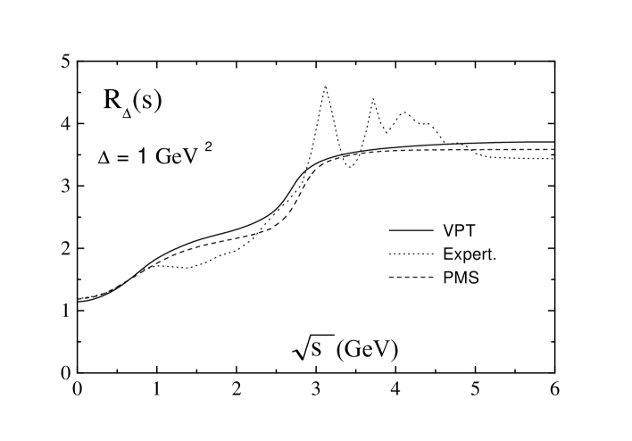
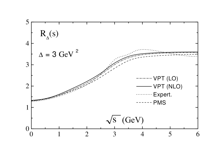
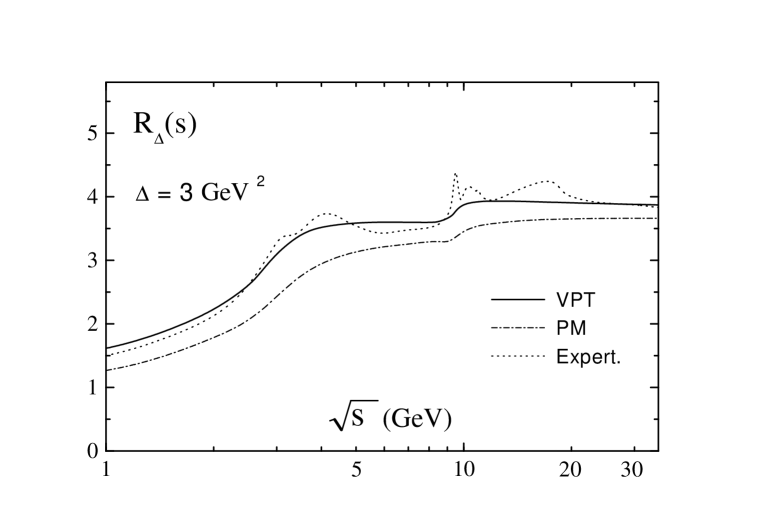
Our results are presented in Figs. 1–4. In Figs. 1 and 2 we plot the smeared functions $R_{\Delta}(s)$ for $\Delta=1~{}{\rm GeV}^{2}$ and $\Delta=3~{}{\rm GeV}^{2}$ respectively. The solid line is the VPT next-to-leading order (NLO) result which was normalized at the $\tau$ lepton scale. To this end, we use the method of description of the $\tau$ decay suggested in Refs. [21, 22] and take here the following experimental average value $R_{\tau}=3.642\pm 0.021$ [23] as input. To demonstrate the fact of stability we show in Fig. 2 the leading-order (LO) VPT result. In these figures we also plot, as dashed curves, results obtained by using the principle of minimal sensitivity (PMS) to optimize the third order of the perturbative expansion and the smeared experimental data, as dotted lines, taken from Ref. [6]. For $\Delta=1~{}{\rm GeV}^{2}$ the resonances in the $e^{+}e^{-}$ annihilation cross-section are not smeared enough, since there are some peaks in the region of $J/\psi$ meson family. With increase in the value of $\Delta$ the resonance structure is smoothed and finally disappears. For a wider interval of energy up to 35 GeV the smeared experimental data have been recently obtained in Ref. [7]. We represent these data and our NLO result in Fig. 3, where we also show the parton model (PM) result as the dash-dotted curve.

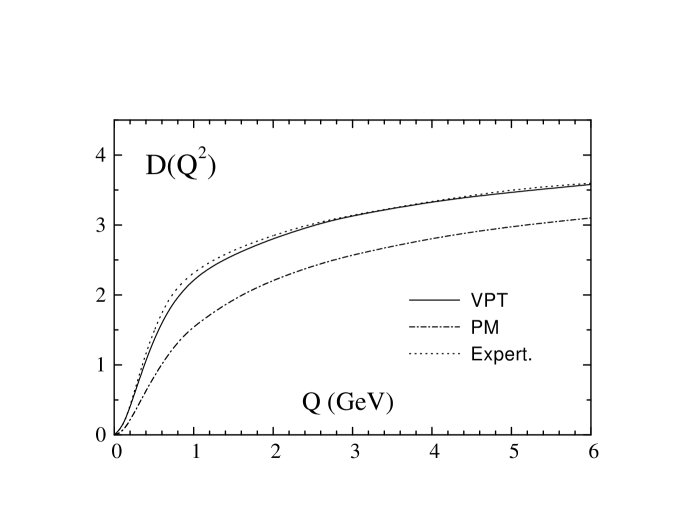
The $D$-function defined in the Euclidean region for positive momentum $Q^{2}$ is a smooth function and thus it is not necessary to apply any “smearing” procedure in order to have the possibility of comparing theoretical results with experimental data. We plot our results in Fig. 4, where we also show the experimental curve taken from Ref. [5] and parton model prediction. The shape of the infrared tail of the $D$-function is sensitive to the value of the masses of the light quarks (the smeared $R_{\Delta}(s)$ function for $\Delta\simeq 1\mbox{--}3\;{\rm{GeV}}^{2}$ is less sensitive to the value of these masses). In our calculations we use the following masses $m_{u}=m_{d}=250\,{\rm{MeV}}$, $m_{s}=400\,{\rm MeV}$, $m_{c}=1.3\,{\rm GeV}$, and $m_{b}=4.7\,{\rm GeV}$, which are close to the constituent quark masses and incorporate, therefore, some nonperturbative effects. Practically the same values of the quark masses were used to describe the experimental data in Refs. [17, 25].

4. In this paper we have applied the nonperturbative method of the $a$-expansion to describe the single-argument functions which are directly connected with the experimental data describing $e^{+}e^{-}$ annihilation into hadrons. An important feature of this approach is the fact that for sufficiently small value of the coupling (the ultraviolet region of momentum) it automatically reproduces the conventional perturbative results. We emphasize that the entire high-energy physics regime is accessible within this approach. Even going into the infrared region of small momentum, where the running coupling becomes large and the standard perturbative expansion fails, the $a$-expansion parameter remains small and we do not find ourselves outside the region of validity of the approach.

We have considered two quantities that are convenient both for the theoretical analysis and for the model-independent comparison with experimental data. The first one is the Poggio-Quinn-Weinberg smeared function, $R_{\Delta}(s)$, defined in the Minkowskian region. The second one is the Adler $D$-function defined in the Euclidean region. It should be emphasized that the smeared quantity $R_{\Delta}(q^{2})$ and the $D$-function have different sensitivity to QCD parameters. For example, in contrast to the smeared function taken with a reasonable value of the parameter $\Delta$ the shape of the $D$-function in the infrared region is very sensitive to the values of the masses of the light quarks. At the same time, for $\Delta\simeq 2\mbox{--}3\,{\rm GeV}^{2}$, the function $R_{\Delta}(s)$ is sensitive to the mass of charmed quark. Thus, these functions can test different parameters of the theory and, in some sense, are complementary to each other.

It should be stressed that in this approach we use the parameters which are included in the Lagrangian and do not introduce any additional model parameters. Nevertheless we found good agreement between our results and the experimental data down to the lowest energy scale. At the same time, note that a straightforward attempt to apply the conventional operator product expansion, which leads to the “condensate” term in the $D$-function, a $\langle\alpha_{s}G^{2}\rangle/Q^{4}$ contribution, is not satisfactory because of the ill-definition of this expansion at small momentum.

REFERENCES

- [1] P.D. Adler, Phys. Rev. D10, 3714 (1974).
- [2] E.C. Poggio, H.R. Quinn and S. Weinberg, Phys. Rev. D13, 1958 (1976).
- [3] I.L. Solovtsov, Phys. Lett. B327, 335 (1994); Phys. Lett. B340, 245 (1994).
- [4] A.N. Sissakian and I.L. Solovtsov, Phys. Lett. A157, 261 (1991); Z. Phys. C54, 263 (1992); A.N. Sissakian, I.L. Solovtsov and O.Yu. Shevchenko, Int. J. Mod. Phys. A9, 1929 (1994); A.N. Sissakian and I.L. Solovtsov, Phys. Part. Nucl. 25, 478 (1994).
- [5] S. Eidelman, F. Jegerlehner, A.L. Kataev, and O. Veretin, Phys. Lett. B454, 369 (1999).
- [6] A.C. Mattingly and P.M. Stevenson, Phys. Rev. D49, 437 (1994).
- [7] S.J. Brodsky, J.R. Peláez and N. Toumbas, Phys. Rev. D60, 037501 (1999).
- [8] T. Barnes and G.T. Ghandour, Phys. Rev. D22, 924 (1980); P.M. Stevenson, Phys. Rev. D30, 1712 (1984); Phys. Rev. D32, 1389 (1985); A. Okopinska, Phys. Rev. D35, 1835 (1987); Phys. Rev. D36, 2415 (1987); T. Stancu and P.M. Stevenson, Phys. Rev. D42, 2710 (1990).
- [9] C.M. Bender, F. Cooper, K.A. Milton, M. Moshe, S.S. Pinsky, and L.M. Simmons Jr., Phys. Rev. D45, 1248 (1992); C.M. Bender, A. Duncan and H.F. Jones, Phys. Rev. D49 4219 (1994); D. Gromes, Z. Phys. C71 347 (1996).
- [10] W.E. Caswell, Ann. Phys. 123, 153 (1979); J. Killingbeck, J. Phys. A14, 1005 (1981).
- [11] P.M. Stevenson, Nucl. Phys. B231, 65 (1984).
- [12] H.F. Jones and I.L. Solovtsov, Phys. Lett. B349, 519 (1995).
- [13] D.V. Shirkov and I.L. Solovtsov, JINR Rapid Comm. No.2[76]-96, 5, hep-ph/9604363; Phys. Rev. Lett. 79, 1209 (1997).
- [14] K.A. Milton and I.L. Solovtsov, Phys. Rev. D55, 5295 (1997).
- [15] K.A. Milton and O.P. Solovtsova, Phys. Rev. D57, 5402 (1998).
- [16] I.L. Solovtsov and D.V. Shirkov, Phys. Lett. B442, 344 (1998).
- [17] D.V. Shirkov and I.L. Solovtsov, talk given at the International Workshop on Collisions from to , Novosibirsk, 1999, hep-ph/9906495.
- [18] K.A. Milton and I.L. Solovtsov, Phys. Rev. D59, 107701 (1999).
- [19] S.G. Gorishny, A.L. Kataev and S.A. Larin, Nuovo Cim. 92A, 119 (1986).
- [20] W.J. Marciano, Phys. Rev. D29, 580 (1984).
- [21] H.F. Jones, I.L. Solovtsov and O.P. Solovtsova. Phys. Lett. B357, 441 (1995).
- [22] H.F. Jones and I.L. Solovtsov, Proceedings of the International Europhysics Conference on High Energy Physics, Brussels, 27 July–2 August, 1995, Editors J. Lemonne, C. Vander Velde, F. Verbeure, World Scientific (Singapore) 1996, p. 242.
- [23] Particle Data Group, C. Caso et al., Eur. Phys. J. C3, 1 (1998).
- [24] See e.g., R. Barate et al., ALEPH Collab., Eur. Phys. J. C4, 409 (1998).
- [25] A.I. Sanda, Phys. Rev. Lett. 42, 1658 (1979).