SNO: Predictions for Ten Measurable Quantities

We calculate the range of predicted values for $10$ quantities that will be measured by the Sudbury Neutrino Observatory (SNO). We use neutrino oscillation solutions (vacuum and MSW; active and sterile neutrinos) that are globally consistent with all available neutrino data and estimate realistic theoretical and experimental uncertainties. The neutral current to charged current double ratio is predicted to be more than $9\sigma$ from the no-oscillation solution for all of the currently favored neutrino oscillation solutions. The best-fit oscillation solutions predict a CC day-night rate difference between $-0.1$% and $+12.5$% and a NC day-night difference $<0.01$%. We present also the predicted range for the first and the second moments of the charged current electron recoil energy spectrum, the charged current, the neutral current, and the $\nu$-$e$ scattering rates, the seasonal dependence of the charged current rate, and the double ratio of neutrino-electron scattering rate to charged current rate.

I Introduction

What can one learn from measurements with the Sudbury Neutrino Observatory (SNO) [1]? What are the most likely quantitative results for each of the different experiments that can be carried out with SNO? The main goal of this paper is to help answer these questions by providing quantitative predictions for the most important diagnostic tests of neutrino oscillations that can be performed with SNO.

SNO is not an experiment. Like LEP and Super-Kamiokande, SNO is a series of experiments. We calculate the currently-favored range of predictions for $10$ quantities that are affected by neutrino oscillations and which SNO will measure. For the impatient reader, we list here the quantities that are sensitive to neutrino oscillations which we investigate (definitions are given later in the text): first and second moments of the recoil energy spectrum, the charged current (CC), the neutral current (NC), and the neutrino-electron scattering rates, the difference between the day and the night rates for both the CC and the NC, the difference in the winter-summer CC rates, the neutral current (NC) to charged current (CC) double ratio, and the neutrino-electron scattering to CC double ratio.

The simultaneous analysis of all the SNO results, measured values and upper limits, will be a powerful technique for constraining neutrino oscillation parameters. As an initial step in this direction, we analyze the combined results for five especially informative pairs of oscillation parameters.

A SNO reactions

The SNO collaboration will study charged current (CC) neutrino absorption by deuterium,

$$\nu_{e}+d\to p+p+e^{-}\ ,$$ (1)

neutral current (NC) neutrino disassociation of deuterium,

$$\nu_{x}+d\to n+p+\nu^{\prime}_{x}\ ,\quad(x=e,\mu,\,\tau),$$ (2)

and neutrino-electron scattering (ES),

$$\nu_{x}+e^{-}\to\nu^{\prime}_{x}+e^{-}\ ,\quad(x=e,\mu,\,\tau).$$ (3)

The energy of the recoil electrons can be measured for the CC reaction, Eq. (1), and also for the ES reaction, Eq. (3). For both these reactions, the operating energy threshold for the recoil electrons may be of order $5$ MeV. The threshold for the NC reaction, Eq. (2), is $2.225$ MeV. Just as for radiochemical solar neutrino experiments, there is no energy discrimination for the NC reaction.

The Kamiokande [2] and Super-Kamiokande experiments [3] have performed precision studies of solar neutrinos using the neutrino-electron scattering reaction, Eq. (3). SNO will be the first detector to measure electron recoil energies as a result of neutrino-absorption, Eq. (1). We have presented in Ref. [4] detailed predictions of what may be observed with SNO for the CC (absorption) reaction.

If there are no neutrino oscillations, i.e., $\phi(\nu_{e})=\phi({\rm total})$, then the ratios of the event rates in the SNO detector are calculated to be approximately in the following proportions: CC:NC:ES = 2.05:1.00:0.19, i.e., the number of CC events is expected to exceed the number of $\nu$-$e$ scattering events by about a factor of $11$. Since the NC efficiency is likely to be only about a half of either the CC or the ES efficiency [1] and currently favored oscillation solutions give $\phi(\nu_{e})\sim\phi({\rm total})$, the observed ratio of events in the SNO detector may actually be reasonably close to: CC:NC:ES $\sim 2.0:0.5:0.2$.

In thinking about what SNO can do, it is useful to have in mind some estimated event rates for a year of operation. The Super-Kamiokande event rate [3] for neutrino electron scattering is $0.475$ times the event rate that is predicted by the standard solar model [5]. If there are no neutrino oscillations and the total solar neutrino flux arrives at earth in the form of $\nu_{e}$ with a ⁸B neutrino flux of $0.475$ times the standard model flux, then one expects about $4.4\times 10^{3}$ CC events per year in SNO above a $5$ MeV threshold and about $1.1\times 10^{3}$ NC events, while there should only be about $415$ ES events. The above rates were calculated for a $5$ MeV CC and ES energy threshold and for a $50$% detection efficiency for NC events. For an $8$ MeV threshold, the estimated CC rate is about $45$% of the rate for a $5$ MeV threshold and the ES rate is only about $28$% of the $5$ MeV threshold rate. For the currently favored oscillation solutions, the expected CC rates are typically of order $80$% of the rates cited above and the NC rates are about a factor of two or three higher.

B What do we calculate?

In this paper, we calculate the likely range of quantities that are measurable with SNO using a representative sample of neutrino parameters from each of the six currently allowed $99$% C.L. domains of two-flavor neutrino oscillation solutions. In other words, we explore what can be learned with SNO, assuming the correctness of one of the six neutrino oscillation solutions [4, 6] that is globally consistent at $99$% C.L. with all of the solar neutrino experiments performed so far (chlorine [7], Kamiokande [2], Super-Kamiokande [3], Sage [8], and GALLEX [9]).

TABLE I.: Best-fit global oscillation parameters. The differences of the squared masses are given in ${\rm eV^{2}}$. The survival probabilities that correspond to these best-fit solutions are shown in Fig. 1 and Fig. 2. Results are taken from Ref. [4]

Scenario	$\Delta m^{2}$	$\sin^{2}(2\theta)$
LMA	$2.7\times 10^{-5}$	$7.9\times 10^{-1}$
SMA	$5.0\times 10^{-6}$	$7.2\times 10^{-3}$
LOW	$1.0\times 10^{-7}$	$9.1\times 10^{-1}$
${\rm VAC_{S}}$	$6.5\times 10^{-11}$	$7.2\times 10^{-1}$
${\rm VAC_{L}}$	$4.4\times 10^{-10}$	$9.0\times 10^{-1}$
${\rm Sterile}$	$4.0\times 10^{-6}$	$6.6\times 10^{-3}$

Table I lists the mixing angles and differences of mass squared for the six global best-fit solutions. Figure 1 and Figure 2 show the survival probabilities of the best-fit solutions as a function of energy

FIG. 1.: The survival probabilities as a function of neutrino energy. For each of the six best-fit globally acceptable neutrino oscillation solutions discussed in Ref. [4], the figure shows the survival probability for electron type neutrinos as a function of energy. The results are averaged over one year.

For each measurable quantity $i$, we express our predictions based upon neutrino oscillation models in terms of the value predicted by an oscillation scenario divided by the value predicted by the combined standard electroweak model and the standard solar model. Thus for each measured quantity, $i$ (like CC or NC event rate), we evaluate the expected range of the reduced quantity $[i]$

$$[i]~{}\equiv~{}\frac{{\rm(Observed~{}Value)_{i}}}{{\rm(Standard~{}Model~{}Value)_{i}}}.$$ (4)

The reduced quantity $[i]$ is by construction independent of the absolute value of the solar neutrino flux, which is used in calculating both the numerator and denominator of Eq. (4).

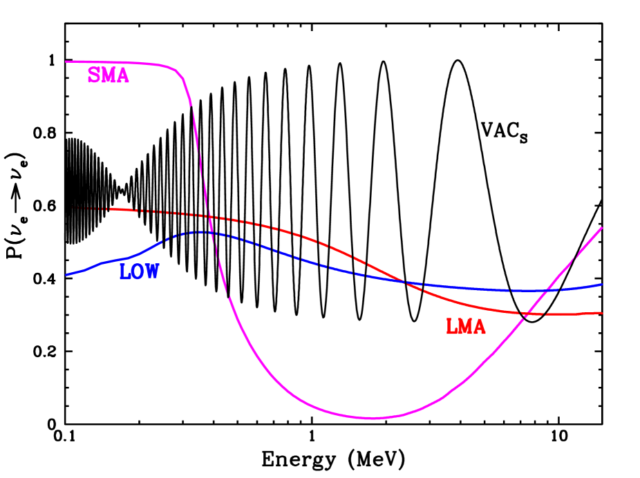
FIG. 2.: Comparison of survival probabilities. For four of the best-fit oscillation solutions, the survival probabilities are compared using a linear energy scale. The differences in the energy dependence of the survival probability between the high energy region, $\sim 8$ MeV, and the low energy region, $\leq 1$ MeV, can be seen clearly on this figure. The MSW Sterile solution has an energy dependence similar to the SMA solution. For clarity, we have omitted the VAC_L solution. The parameters of the best-fit solutions are given in Table I.

What fluxes are used in calculating the predicted rates (e.g., for charged current or electron-neutrino interactions) implied by different neutrino scenarios? We determine the best-fit ratio of the observed neutrino flux to the standard model flux by fitting to the Super-Kamiokande rate and observed recoil electron spectrum. The procedure is described in Sec. III following Eq. (12) and Eq. (13) (see especially the definition of $f(^{8}B)$). We have not included explicit uncertainties in determining $f(^{8}B)$ for a given pair of neutrino variables, $\Delta m^{2}$ and $\sin^{2}2\theta$, but we instead have allowed $f(^{8}B)$ to range over the wide set of values obtained by applying our best-fit procedure at each point in the currently-allowed neutrino-parameter space.

As we shall see, the most powerful diagnostics of neutrino oscillations are formed by considering the reduced double ratio of two measurable quantities, $i$ and $j$, as follows:

$${[i]\over[j]}~{}\equiv~{}\frac{{\rm(Observed~{}Value)_{i}/(Standard~{}Model~{}Value)_{i}}}{{\rm(Observed~{}Value)_{j}/(Standard~{}Model~{}Value)_{j}}}.$$ (5)

For example, the reduced double ratio of NC to CC rates is not only independent of the absolute flux of the solar neutrinos but is also insensitive to some experimental and theoretical uncertainties that are important in interpreting the separate [NC] and [CC] rates.

We describe how we evaluate the uncertainties in Sec. II. All of the calculated departures from the standard model expectations are small except for the double ratio of NC to CC, [NC]/[CC]. Therefore, the theoretical and the experimental uncertainties are important.

We present in Sec. III the results predicted by the six oscillation solutions for the first and second moments of the shape of the CC recoil electron energy distribution. We summarize in Sec. IV the principal predictions for the CC rate, in Sec. V the predictions for the neutral current rate, and in Sec. VI the predictions for the neutrino-electron scattering rate. We then calculate the detailed predictions of the most important double ratios, the NC to charged current ratio, [NC]/[CC], in Sec. VII and the neutrino-electron scattering to CC ratio, [ES]/[CC], in Sec. VIII.

Up to this point in the paper, i.e., through Sec. VIII, we only discuss time-averaged quantities. In Sec. IX, we present the predictions for the CC of the difference between the event rate observed at night and the event rate observed during the day. For the NC rate, there is also a small difference predicted between the night rate and the day rate if the MSW Sterile solution is correct. We analyze in Sec. X the seasonal effects in the CC rate.

Section XI is a pairwise exploration of the discriminatory power gained by analyzing simultaneously the predictions and the observations of different smoking-gun indicators of neutrino oscillations. We consider in this section the joint analysis of variables like [NC]/[CC] versus the first moment of the CC energy spectrum, the day-night difference, or the neutrino-electron scattering rate. In Sec. XII, we summarize and discuss our principal conclusions. Since we evaluate so many different effects, we give in Sec. XIII our personal list of our top four conclusions.

C How should this paper be read?

We recommend that the reader begin by looking at the figures, which give a feeling for the variety and the size of the various quantities that can be measured with SNO. Then we suggest that the reader jump directly to the end of the paper. The main results of the paper are presented in this concluding section; the summary given in Sec. XII can be used as a menu to guide the reader to the detailed analyses that are of greatest interest to him or to her.

This is the fifth in a series of papers that we have written on the potential of the Sudbury Neutrino Observatory for determining the properties of neutrino oscillations. The reader interested in details of the analysis may wish to consult these earlier works [4, 10, 11, 12], which also provide a historical perspective from which the robustness of the predictions can be judged. The present paper is distinguished from its predecessors mainly in the specificity of the predictions (representative $99$% C.L. predictions for each of the six currently acceptable neutrino oscillation scenarios) and in the much larger number of measurable quantities for which we now make predictions.

Recent review articles summarize clearly the present state of neutrino physics [13, 14] and neutrino oscillation experiments and theory [6, 15, 16, 17]. Three and four flavor solar neutrino oscillations are discussed in Refs. [18, 19] and references cited therein. The fundamental papers upon which all of the subsequent solar neutrino oscillation work is based are the initial study of vacuum oscillations by Gribov and Pontecorvo [20] and the initial studies of matter oscillations (MSW) by Mikheyev, Smirnov, and Wolfenstein [21]. In addition to the by-now conventional scenarios of oscillations into active neutrinos, we also consider oscillations into sterile neutrinos [6, 19, 22, 23, 24, 25, 26].

II Estimation of uncertainties

In this section, we describe how we calculate the uncertainties for different predicted quantities. Since the interpretation of future experimental results depends upon the assigned uncertainties, we present here a full description of how we determine the errors that we use in the remainder of the paper.

Let $X$ represent the predicted quantity of interest, which may be, for example, the first or second moment of the recoil energy spectrum, the neutrino-electron scattering rate, the double ratio of neutral current to charged current rate, the double ratio of neutrino-electron scattering to charged current rate, or the difference between the day rate and the night rate. The method that we adopt is the same in all cases. We evaluate $X$ with two different assumptions about the size or behavior of a particular input parameter (experimental or theoretical). The different assumptions are chosen so as to represent a definite number of standard deviations from the expected best-estimate. The difference between the values of $X$ calculated for the two assumptions determines the estimated uncertainty in $X$ due to the quantity varied.

To clarify what we are doing, we illustrate the procedure with specific examples. We begin by describing in Sec. II A how we calculate theoretical uncertainties and then we discuss the detector-related uncertainties in Sec. II B.

A Theoretical uncertainties

FIG. 3.: The calculated standard recoil electron energy spectra in SNO. The figure shows the predicted shapes, $\lambda(T)$, of the normalized recoil electron energy spectra that are obtained by assuming that no oscillations occur and by using the standard (undistorted) ⁸B neutrino energy spectrum. The spectra are given as a function of the true electron kinetic energy in MeV, $T_{\rm e,~{}true}$, not the apparent energy measured by the detector. The spectra shown do not include instrumental effects such as the finite energy resolution of the detector or uncertainties in the absolute energy scale. The dotted curve represents the recoil electron spectrum due to neutrino-electron scattering and the solid curve represents the electron spectrum produced by neutrino absorption (CC reactions) on deuterium.

We discuss in this subsection the uncertainties related to the ⁸B neutrino energy spectrum, the neutrino interaction cross sections, and the $hep$ solar neutrino flux. The standard shape of the ⁸B neutrino spectrum has been determined from the best-available experimental and theoretical information [27].

Figure 3 shows the recoil electron energy spectra calculated for neutrino-electron scattering and for charged current (absorption) on deuterium that were calculated using the undistorted standard ⁸B neutrino energy spectrum. The recoil energy spectra produced by neutrino-electron scattering and by neutrino absorption are very different. One can easily see from Fig. 3 how the location of the threshold for CC events at $5$ MeV (before the peak) or at $8$ MeV (after the peak) could give rise to different sensitivities to uncertainties in, e.g., the energy resolution function. This is one of the reasons why we have calculated in the following sections predicted values and uncertainties for two different thresholds. For neutrino-electron scattering, the energy distribution decreases monotonically from low to high energies; this uniform behavior decreases the sensitivity, relative to the absorption process, to some uncertainties.

Two extreme deviations from the shape of the standard spectrum were also determined using the best-available information [27]; these extreme shapes represent the total effective $\pm 3\sigma$ deviations. We calculate the quantities $X$ that will be measured by SNO using the standard ⁸B spectrum and the effective $3\sigma$ different spectra and determine from the following formula the associated uncertainty due to the shape of the ${}^{8}B$ spectrum. Thus

$$\sigma_{X}({\rm{}^{8}B~{}spectrum})~{}=~{}6^{-1}[~{}|\,X(+3\sigma~{}{\rm spectrum})~{}-~{}X(-3\sigma~{}{\rm spectrum})\,|~{}].$$ (6)

TABLE II.: Neutrino Interaction Cross Sections on Deuterium. The table gives, in units of $10^{-42}~{}{\rm cm^{2}}$, the neutrino charged current (CC) and neutral current (CC) cross sections for deuterium. The cross sections calculated by different authors (shown in column 1) have been averaged over a standard ⁸B neutrino energy spectrum. For the CC reactions, a $5$ MeV threshold for the recoil electron energy was assumed and the energy resolution function for SNO was approximated by Eq. (10) and Eq. (11). The last column gives the calculated ratios of the NC to CC ratios.

Authors	CC	NC	NC/CC
KNa	0.979	0.478	0.488
YHHb	0.923	0.449	0.486
EBLc	0.889	…

Table II lists the three relatively recent calculations for the charged current absorption cross sections on deuterium, by Ying, Haxton, and Henley (YHH) [29], by Kubodera and Nozawa (KN) [28], and by Bahcall and Lisi (BL) [11]; the YHH and KN calculations use potential models and BL used an effective range treatment. For the neutral current cross sections, only the YHH and KN cross sections are available. If the quantity $X$ involves the neutral current, then we define the $1\sigma$ uncertainty by evaluating

$$\sigma_{X}({\rm NC~{}cross~{}section})~{}=~{}|~{}X({\rm YHH~{}cross~{}section})~{}-~{}X({\rm KN~{}cross~{}section})~{}|.$$ (7)

Using the values given in Table II, we define analogous $1\sigma$ uncertainties for quantities associated with the CC and the double ratio, [CC]/[NC].

There is no principle of physics that enables one to set a rigorous error estimate based upon the cross section calculations summarized in Table II. As a practical and plausible estimate for this paper, we have used the average of the detailed Kubodera and Nozawa and Ying, Haxton, and Henley calculations as our best estimate and taken the difference between these two cross sections to be an effective $1\sigma$ uncertainty (see also the discussion by Butler and Chen in Ref. [31]). Experimental measurements with reactor anti-neutrinos are not yet sufficiently accurate to refine and choose between different theoretical calculations (see results in Ref. [32]). Had we adopted the Ellis, Bahcall, and Lisi effective range calculation as the lower limit instead of the Ying et al. result, we would have obtained for the CC an uncertainty of $9.7$% instead of $5.8$%. Earlier, Bahcall and Kubodera [33] estimated an effective $3\sigma$ uncertainty of $\pm 10$% for the neutral current cross section by calculating cross sections with and without meson-exchange corrections, using different sets of coupling constants, and two different nuclear potentials.

The nuclear fusion reaction that produces $hep$ neutrinos cannot be calculated or measured reliably [34, 35]. The shape of the electron recoil energy distribution measured by Super-Kamiokande can be significantly influenced by the rare high-energy $hep$ neutrinos [3, 34, 35, 36]. In this paper, we need to evaluate the uncertainty in a variety of quantities $X$ due to the unknown $hep$ flux. We use the results given in the last column of Table 3 of Ref. [4], which lists the range of $hep$ fluxes that correspond to different oscillation solutions that lie within the $99$% ($\sim 2.5\sigma$) C.L. allowed range. Given the range of listed $hep$ fluxes, we make the plausible but not rigorous estimate that the effective $1\sigma$ uncertainty in the $hep$ flux is currently between $0$ and $20$ times the nominal standard estimate of $2.15\times 10^{3}~{}{\rm cm^{-2}s^{-1}}$ ($0.0004$ the best-estimate ⁸B flux). Therefore, we evaluate the uncertainty due to the increase of the $hep$ flux above the nominal standard value from the following relation

$$\sigma_{X}~{}hep~{}{\rm flux}~{}=~{}|~{}X(20\times\phi(hep,{\rm~{}BP98}))~{}-~{}X(0\times\phi(hep,{\rm~{}BP98}))~{}|.$$ (8)

The uncertainty in the $hep$ flux is asymmetric (negative fluxes are not physical). We calculate the lower error by replacing $20\times\phi(hep,{\rm~{}BP98})$ in Eq. (8) by $1\times\phi(hep,{\rm~{}BP98})$. The lower error corresponds to decreasing the $hep$ flux to zero. The uncertainty in the $hep$ flux does not dominate the error budget for any of the quantities we discuss. If the reader wishes to treat differently the $hep$ flux uncertainty, this can be done easily by using the individual uncertainties in Table III.

For the standard solar model (SSM), the nominal ratio of the $hep$ neutrino flux to the ⁸B neutrino flux is $4\times 10^{-4}$ [5]. Of all the quantities we consider in this paper, the first and second moments of the electron recoil energy spectrum, which are discussed in Sec. III, are most sensitive to the $hep$ flux. For a nominal SSM $hep$ flux, the first moment is shifted by $3\times 10^{-4}$ relative to the first moment computed with a zero $hep$ flux. The corresponding change for the standard deviation of the recoil energy spectrum is $2\times 10^{-3}$. Thus the $hep$ flux of the standard solar model is of negligible importance for all of the quantities we calculate in this paper. The $hep$ neutrino flux will have a significant effect on the quantities computed here only if the flux exceeds the nominal standard value by at least an order of magnitude.

Super-Kamiokande and SNO will obtain somewhat tighter constraints on the $hep$ flux. Measurements of the seasonal variations of the ⁷Be flux will test vacuum neutrino scenarios that have a small $hep$ flux but an appreciable distortion of the Super-Kamiokande recoil energy spectrum [37]. Since $\sigma_{X}(hep{\rm~{}flux})$ is linearly proportional to the allowed range of the $hep$ flux, a reduction in the allowed range by, for example, a factor of two will reduce the estimated value of $\sigma_{X}(hep{\rm~{}flux})$ by a factor of two.

For neutrino-electron scattering, the situation is very different. The interaction cross sections can be calculated precisely including even the small contributions from radiative corrections. We use in this work the cross sections calculated in Ref. [38]; the uncertainties in these radiative corrections are negligible for our purposes.

In the following sections, we often quote fractional uncertainties in percent. We define the fractional uncertainty to be the one sigma difference divided by the average of the two values used to obtain the error estimate. Thus the fractional uncertainty due to an increase in the poorly known $hep$ flux is

$$\delta X(hep{\rm~{}flux})~{}=~{}100\times{{2\sigma_{X}(hep{\rm~{}flux})}\over{|~{}X(20\times\phi(hep,{\rm~{}BP98}))~{}+~{}X(0\times\phi(hep,{\rm~{}BP98}))~{}|}}.$$ (9)

B Detector-related uncertainties

There are important detector-related uncertainties that can only be determined by detailed measurements with the SNO detector and by careful Monte Carlo simulations. Perhaps the most dangerous of these uncertainties are the misidentification uncertainties, the incorrect classification of CC, ES, and NC events. These errors do not cancel in the double ratios discussed later in this paper, such as [ES]/[CC] and [NC]/[CC].

SNO is a unique detector. No other detector has previously separated the CC and the NC reactions. The only reliable way of estimating the effects of the confusion between different neutrino reactions is to use the full-scale Monte Carlo simulation that is under development by the SNO collaboration. Since the SNO collaboration will measure the NC rate in different ways, there will also ultimately be internal cross checks that will limit the error due to the NC contamination of the CC and the ES rates. The ES contamination of CC quantities like the spectrum distortion or the day-night effect is likely to be small, since neutrino-electron scattering is strongly peaked in the forward direction and is estimated to be detected at only $\sim 0.1$ the CC rate. Hopefully, misclassification errors will have only minor effects and will be well described by the SNO Monte Carlo simulations. But, the reader should keep in mind that the errors estimated in this paper are lower limits; they represent errors that we can estimate quantitatively without a large Monte Carlo simulation. We will not consider errors due to misclassification of neutrino event in the reminder of this paper.

One can make reasonable guesses for other important experimental uncertainties using the experience gained from previous water Cherenkov solar neutrino experiments and preliminary Monte Carlo studies of how the SNO detector will perform. The most important of these quantities that need to be determined, together with their uncertainties, are the energy resolution, the absolute energy scale, the detector efficiencies (for energetic electrons and for neutral current reactions), and the energy threshold for detecting CC events. In what follows, we will adopt the preliminary characterizations for these detector-related uncertainties used by Bahcall and Lisi [11]. We now summarize briefly our specific assumptions for these uncertainties.

Let $T_{e}^{\prime}$ be the true electron recoil kinetic energy and $T_{e}$ be the kinetic energy measured by SNO. We adopt the resolution function $R(T_{e}^{\prime},\,T_{e})$,

$$R(T_{e}^{\prime},\,T_{e})=\frac{1}{\sigma(T_{e}^{\prime})\sqrt{2\pi}}\exp{\left[-\frac{(T_{e}^{\prime}-T_{e})^{2}}{2\sigma(T_{e}^{\prime})^{2}}\right]},$$ (10)

with an energy-dependent one-sigma width $\sigma(T^{\prime}_{e})$ given approximately by

$$\sigma(T^{\prime}_{e})=(1.1\pm 0.11)\sqrt{\frac{T^{\prime}_{e}}{10{\rm\ MeV}}}\,{\em MeV}.$$ (11)

We adopt a conservative estimate for the $1\sigma$ absolute energy error of $\pm 100$ keV. We will assume, for illustrative purposes, that the threshold for detecting recoil electrons is a total energy of $5$ MeV or $8$ MeV.

For specificity, we assume [11] that the neutral current detection efficiency is $0.50\pm 0.01$ and that the detection efficiency for recoil electrons above threshold is approximately $100$%.

C Summary of uncertainties

In this subsection, we present a convenient table that summarizes the estimated uncertainties for the different physical quantities that are discussed in detail in the following sections of the paper. It may be useful to the reader to refer back to this summary table from time-to-time while considering the detailed presentations.

TABLE III.: Fractional uncertainties in percent for some quantities that are measurable with the SNO detector. Here $\delta X=100\sigma_{X}/X$. The different quantities are defined in the following sections: $T$ and $\sigma$ are the first and second moments, respectively; [CC], [NC], and [ES] are the reduced charged current, neutral current, and neutrino-electron scattering rates, respectively; and [NC]/[CC] and [ES]/[CC] are the neutral current to charged current and neutrino-electron scattering to charged current double ratios, respectively. For CC reactions, a $5$ MeV threshold was assumed for the energy of the recoil electrons. The statistical uncertainties are computed assuming $5000$ CC events, $1219$ NC events, and $458$ ES events. We assumed a NC detection uncertainty of $1\sigma=2$%. We do not include uncertainties due to misclassification of neutrino events.

$Source$	$\delta T$	$\delta\sigma$	$\delta[CC]$	$\delta[NC]$	$\delta[ES]$	$\delta[NC]/[CC]$	$\delta[ES]/[CC]$
$Energyresolution$	$0.3$	$1.4$	$0.4$	$\sim 0$	$0.1$	$0.4$	$0.3$
$Energyscale$	$0.8$	$1.1$	$1.5$	$\sim 0$	$0.5$	$1.5$	$1.0$
$B8spectrum$	$0.4$	$0.8$	$1.9$	$1.6$	$1.4$	$0.3$	$0.6$
$Cross-section$	$0.03$	$0.15$	$5.8$	$6.4$	$\sim 0$	$0.4$	$5.8$
$Statistics\leavevmode\leavevmode\hbox{${}^{\rm a}$}$	$0.35$	$1.1$	$1.4$	$2.9$	$4.7$	$3.2$	$4.9$
$hep\leavevmode\leavevmode\hbox{${}^{\rm b}$}$	$0.8$	$0.8$	$2.3$	$2.2$	$1.6$	$0.1$	$0.7$
$Total$	$1.3$	$2.4$	$6.7$	$7.4$	$5.2$	$3.6$	$7.6$

Table III shows the fractional uncertainties in percent that we have estimated for different measurable quantities. The quantities in the Table are defined in the following sections. The counting uncertainties are determined assuming that a total of $5000$ events are measured in the CC mode; the number of NC and neutrino-electron scattering events are then about $1219$ and $458$, respectively. For an $8$ MeV electron energy threshold rather than the $5$ MeV threshold used in computing Table III, the statistical uncertainties would be increased by about $50$% for the purely CC quantities like $\delta T$, $\delta\sigma$, and [CC]. For quantities related to the ES rate, the statistical uncertainties would be increased by a factor of about $1.9$ by raising the electron recoil energy threshold to $8$ MeV. The statistical error is expected, for an $8$ MeV threshold, to dominate the uncertainty in the ES rate.

There will be additional contributions to the statistical errors from background sources; these uncertainties can only be determined in the future from the detailed operational characteristics of the SNO detector. For example, the background from the CC events will increase the estimated statistical error for the neutrino-electron scattering events; the amount of the increase will depend upon the angular width of the peak in the $\nu$-$e$ scattering function. We have not estimated uncertainties for the day-night asymmetry, $A$, defined by Eq. (32) since a detailed knowledge of the detector is required to estimate the small uncertainties in $A$.

The errors due to the uncertainties in the $hep$ flux are asymmetric. We show in Table III only the upper limit uncertainties for $hep$. The lower limit uncertainties are negligibly small for $hep$, since the standard model flux ratio for $hep$ to ⁸B is $0.0004$.

The actual background rates in the SNO detector are not yet known and may differ considerably from the rates that were estimated prior to the building of the observatory. We have therefore not attempted to include background uncertainties, although these may well be important for some of the quantities we calculate.

For both the CC ratio of measured to standard model rate, [CC], and the similarly defined neutral current ratio, [NC], Table III shows that the absolute value of the neutrino cross section is the dominant source of uncertainty. This uncertainty almost entirely cancels out in the double ratio of ratios, [NC]/[CC]. The absolute energy scale and the value of the $hep$ neutrino energy flux are the largest estimated uncertainties for the first moment of the CC recoil energy spectrum, $\langle T\rangle$. Counting statistics, assuming a total of $5000$ CC events, is estimated to be the most important uncertainty for the neutrino-electron scattering ratio, [ES], and the neutral current to charged current double ratio [NC]/[CC].

In the subsequent discussion, we follow the frequently adopted practice of combining quadratically the estimated $\sigma$’s from different sources, including theoretical errors on cross sections and on the $hep$ flux. If the reader prefers to estimate the total uncertainty using a different prescription, this can easily be done using the individual uncertainties we present.

III The shape of the CC electron recoil energy spectrum

In this section, we make use of the fact that solar influences on the shape of the ⁸B neutrino energy spectrum are only of order $1$ part in $10^{5}$ [39], i.e., are completely negligible. Therefore, we compare all of the neutrino oscillation predictions to the calculated results obtained using an undistorted neutrino spectrum inferred from laboratory data [27].

Figure 3 shows as a solid line the calculated CC electron recoil energy spectrum that would be produced by an undistorted ⁸B neutrino energy spectrum. The result shown in Fig. 3 does not include instrumental effects such as the energy response of the detector, but best-estimates of the instrumental effects (see discussion in Sec. II B) are included in the results given here and in the following sections.

It is useful in thinking about the shapes of the different electron recoil energy spectra to consider the ratio, $R(E_{e})$, of the electron energy spectrum produced by a distorted neutrino spectrum to the spectrum that is calculated assuming a standard model neutrino energy spectrum [40]. We define

$$R(E_{e})=\frac{f{\rm(^{8}B)}N_{B}(E_{e})+f(hep)N_{hep}(E_{e})}{N^{\rm SSM}_{B}(E_{e})+N^{\rm SSM}_{hep}(E_{e})}$$ (12)

where $f(^{8}B)$ is the ratio of the true ⁸B neutrino flux that is created in the sun to the standard solar model ⁸B neutrino flux, i.e., $f(^{8}B)=\phi(^{8}B)_{\rm true}/\phi(^{8}B)_{\rm SSM}$. The quantity $f(hep)$ is similarly defined as the ratio of true to standard solar model $hep$ flux. $N_{B}^{\rm SSM}(E_{e})$ is the number of events in a 0.5 MeV energy bin centered at $E_{e}$ and calculated for the SSM ${\rm{}^{8}B}$ neutrino flux without oscillations. $N_{B}(E_{e})$ is the same quantity with oscillations taken into account. $N^{\rm SSM}_{hep}(E_{e})$ and $N_{hep}(E_{e})$ are the corresponding numbers for the $hep$ flux. We have included the instrumental effects as described in Sec. II B.

We determine the best-fit value of $f({\rm{}^{8}B})$ and $f(hep)$ for each pair of values of the oscillation parameters, $\Delta m^{2}$ and $\sin^{2}2\theta$, by comparing the theoretical predictions with the total rate and the recoil electron energy spectrum of Super-Kamiokande [3, 4]:

$$f_{B}=f_{B}(\Delta m^{2},\sin^{2}2\theta),~{}~{}~{}~{}f_{hep}=f_{hep}(\Delta m^{2},\sin^{2}2\theta).$$ (13)

The uncertainties in the values of $f({\rm{}^{8}B})$ and $f(hep)$ are reflected in the allowed range of $\Delta m^{2}$ and $\sin^{2}2\theta$, but are not included explicitly in Table III.

FIG. 4.: The relative CC recoil energy spectra for six oscillation solutions. The figure shows the rates, $R(E_{e})$, predicted by different best-fit oscillation solutions as a function of the electron recoil energy, $E_{e}$, divided by the rate predicted by the standard solar model and no neutrino oscillations. The oscillation solutions are described in Table I. The highest energy bin represents the average value of $R(E_{e})$ for electron energies between $14$ MeV and $20$ MeV. We use the best-fit $hep$ flux found for each neutrino oscillation scenario, which affects the result in the highest energy bin. The range of $hep$ fluxes is given in Table 3 of Ref. [4].

Figure 4 shows the ratio $R(E_{e})$ calculated for the six best-fit oscillation solutions. The values of $R(E_{e})$ are given in $0.5$ MeV bins except for the last energy bin, where we include all CC events that produce recoil electrons with observed energies above $14$ MeV. Only a few events (less than $1$% of the total number of CC events) are predicted [4] to lie above $14$ MeV since the ⁸B neutrino energy spectrum barely extends beyond $14$ MeV and the $hep$ neutrinos, which extend up to $18.8$ MeV, are expected to be very rare.

Ultimately, SNO will measure the detailed shape of the CC recoil energy spectrum and compare the measurements with the full predictions of different oscillation scenarios, as illustrated in Fig. 4. Since the neutrino oscillation parameters are continuous variables, there are in principle an infinite number of possible shapes to consider. However, much or most of the quantitative information can be summarized conveniently in the first and second moments of the recoil energy spectrum [12] and we therefore concentrate here on the lowest order moments.

Throughout this section, we use the notation of Bahcall, Krastev, and Lisi [12] (hereafter BKL97), who have defined the first and second moments (average and variance) of the electron recoil energy spectrum from CC interactions in SNO. The explicit expressions are given in Eqs. (11)–(17) of BKL97; they include the energy resolution function of the detector [see Eq. (10) of this paper]. Unlike BKL97, we use as our default recoil energy spectrum $5$ MeV total electron energy, rather than $5$ MeV electron kinetic energy. (We also calculate the moments for an $8$ MeV total electron recoil energy.) When we calculate for the same threshold as BKL97, our results for the no-oscillation solution agree to about $1$ part in $10^{4}$. We use a threshold specified in terms of total electron energy because this variable has become the standard for experimentalists to specify their energy threshold.

We denote by a subscript of “0” the standard value of quantities computed assuming no oscillations occur. In order to compare with the theoretical moments given here, the observed moments should be corrected for any dependence of the detection efficiency upon energy that is determined experimentally.

If there are no oscillations, the first moment of the CC electron recoil kinetic energy spectrum is, for a $5$ MeV total electron energy threshold:

$$\langle T\rangle_{0}=7.422\times(1\pm 0.013)~{}{\rm MeV},$$ (14)

where the estimated uncertainties ($\pm 96$ keV) have been taken from Table III. The result given in Eq. (14) applies for a pure ⁸B neutrino spectrum. If one includes a $hep$ neutrino flux equal to the nominal standard solar model value [5], then the first moment is increased by $2$ keV to $7.424$ MeV. For an $8$ MeV energy threshold, $\langle T\rangle_{0}=9.117$ for a pure ⁸B neutrino energy spectrum and is increased by $3$ keV by adding a nominal $hep$ flux.

The largest estimated contributions to the quoted error in Eq. (14) arise from uncertainties in the energy scale and from the $hep$ reaction, with smaller contributions from the width of the energy resolution function and the shape of the ⁸B neutrino energy spectrum. The total error of the measured value is the same, within practical accuracy, whether or not one includes the statistical uncertainty for $5000$ events.

The first moment has the smallest estimated total error of all the quantities tabulated in Table III.

TABLE IV.: The first moment, $\langle T\rangle$, of the electron recoil kinetic energy spectrum from CC interactions. If there are no oscillations, the expected value of the first moment is $\langle T_{0}\rangle=7.422$ MeV for a 5 MeV total electron energy threshold and $\langle T_{0}\rangle=9.117$ MeV for an 8 MeV energy threshold. The table shows for different neutrino oscillation scenarios the absolute shift, $\Delta T=\langle T\rangle-\langle T\rangle_{0}$, in keV of the first moment of the electron recoil energy spectrum. Results are given for both a 5 MeV and an 8 MeV threshold energy. The different columns give the best-fit shift as well as the minimum and maximum shifts at 99% C.L.

Scenario	${(\Delta T)}_{\rm b.f.}$	${(\Delta T)}_{\rm min}$	${(\Delta T)}_{\rm max}$	${(\Delta T)}_{\rm b.f.}$	${(\Delta T)}_{\rm min}$	${(\Delta T)}_{\rm max}$
	keV	keV	keV	keV	keV	keV
	5 MeV	5 MeV	5 MeV	8 MeV	8 MeV	8 MeV
LMA	8	$-115$	34	4	$-35$	15
SMA	218	50	341	66	15	105
LOW	12	$-17$	63	7	$-5$	25
${\rm VAC_{S}}$	283	$-80$	576	122	40	227
${\rm VAC_{L}}$	21	$-152$	214	236	$-54$	358
${\rm Sterile}$	164	41	265	51	13	83

Table IV presents the best-estimates and the total range of the predictions for the six different two-flavor neutrino scenarios that are globally consistent with all of the available neutrino data. Figure 1 of Ref. [4] shows, at $99$% CL, the allowed ranges of the neutrino oscillation parameters of the first five neutrino scenarios listed in Table IV. The abbreviations LMA, SMA, and LOW represent three MSW solution islands and the abbreviations ${\rm VAC_{S}}$ and ${\rm VAC_{L}}$ represent the small-mass and large mass vacuum oscillation solutions, all for oscillations into active neutrinos. The MSW Sterile solution has values for the mixing angle and the square of the mass difference that are similar to the active SMA solution (see discussion in Ref. [4]).

For a 5 MeV electron energy threshold, the predicted shifts in the first moment, $\Delta T=\langle T\rangle-\langle T\rangle_{0}$, range from $-152$ keV to $+576$ keV. The calculational uncertainties and the measurement uncertainties estimated from the expected behavior of SNO, $\pm 96$ keV, are considerably smaller than the total range of shifts, $711$ keV, predicted by the currently allowed set of oscillation solutions. The shift in the first moment may be measurable if either the SMA, ${\rm VAC_{S}}$, ${\rm VAC_{L}}$, or MSW Sterile solutions are correct. For the LMA and LOW solutions, the predicted shifts in the first moment may be too small to obtain a very significant measurement.

A measurement of the first moment with an energy threshold of 5 MeV and a $1\sigma$ accuracy in $\langle T\rangle$ of $100$ keV or better will significantly reduce the allowed range of neutrino oscillation solutions. Table IV shows that a measurement of $\langle T\rangle$ with an energy threshold of 8 MeV will be valuable, although it will provide a less stringent constraint than a measurement with a lower threshold. For an 8 MeV threshold, the currently allowed range is only $412$ keV, almost a factor of two less than the range currently allowed for a 5 MeV threshold.

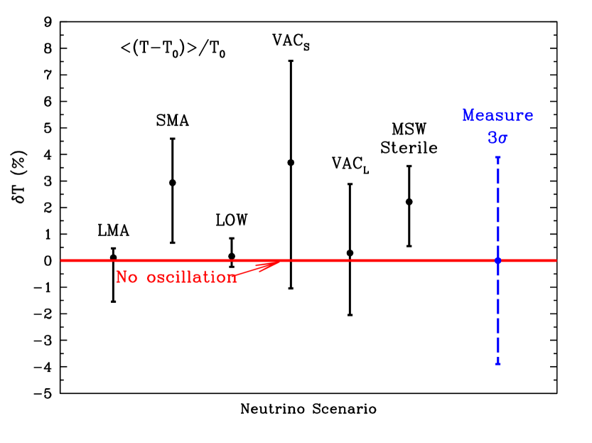
FIG. 5.: The fractional shift in the average electron recoil energy. The figure shows $\delta T$ [defined in Eq. (15)], the fractional change in the average electron recoil energy, $\langle T\rangle$, for the six currently allowed neutrino oscillation solutions. The solid error bars represent the $99$% C.L. for the allowed regions of the six currently favored neutrino oscillation solutions [4]. For an undistorted ⁸B neutrino energy spectrum, the average recoil energy is denoted by $T_{0}$. The dashed error bar labeled “Measure $3\sigma$” represents the uncertainty in interpreting the measurements according to the estimates in Table III, which include the energy resolution, energy scale, ⁸B neutrino energy spectrum, neutrino cross section, counting statistics, and the $hep$ flux. The results are calculated assuming a $5$ MeV threshold for the CC reaction.

Figure 5 shows, for a 5 MeV electron energy threshold, the range of the fractional shift in percent of the first moment,

$$\delta T=\Delta T/\langle T\rangle_{0},$$ (15)

for all six of the oscillation solutions. The results are compared with the no-oscillation solution, $\delta T=0$. The estimated experimental uncertainty in $\delta T$ is about $1$% (see Table III). Only the ${\rm VAC_{S}}$ solutions predict, for about half of their currently allowed solution space, a deviation of $\langle T\rangle$ from the no-oscillation value by more than $3\sigma$. The MSW sterile solution predicts a shift in the first moment that is at most $2.7\sigma$ from the no-oscillation case; this seems like a small shift, but it is notoriously difficult to identify measurable indications of sterile neutrinos that are different from a reduction in the total ⁸B solar neutrino flux [26].

TABLE V.: The standard deviation, $\langle\sigma^{2}\rangle^{1/2}$, of the electron recoil energy spectrum. If there are no oscillations, the expected value of the standard deviation of the electron recoil energy spectrum is $\sigma_{0}=\langle\sigma^{2}\rangle^{1/2}_{0}=1.852$ MeV for a 5 MeV total electron recoil energy threshold and $1.240$ MeV for an 8 MeV energy threshold. The table shows for different neutrino oscillation scenarios the absolute shift of the standard deviation, $\Delta\sigma=\langle\sigma^{2}\rangle^{1/2}-\langle\sigma^{2}\rangle^{1/2}_{0}$, in keV for both a 5 MeV total electron recoil energy threshold and an 8 MeV energy threshold.

Scenario	${(\Delta\sigma)}_{\rm b.f.}$	${(\Delta\sigma)}_{\rm min}$	${(\Delta\sigma)}_{\rm max}$	${(\Delta\sigma})_{\rm b.f.}$	${(\Delta\sigma})_{\rm min}$	${(\Delta\sigma})_{\rm max}$
	keV	keV	keV	keV	keV	keV
	5 MeV	5 MeV	5 MeV	8 MeV	8 MeV	8 MeV
LMA	3	$-19$	9	4	$-13$	11
SMA	23	1	38	23	$3$	34
LOW	3	$-3$	13	2	$-3$	10
${\rm VAC_{S}}$	70	11	136	44	9	76
${\rm VAC_{L}}$	127	$-29$	199	160	$-40$	212
${\rm Sterile}$	19	2	32	14	$-4$	36

Table V presents the predicted shifts in the standard deviation of the CC electron recoil energy distribution (i.e., the square root of the second moment). The calculated no-oscillation value is

$$\sigma_{0}=\langle\sigma^{2}\rangle^{1/2}_{0}=1.852(1\pm 0.024)\,{\rm MeV},$$ (16)

for a 5 MeV total electron recoil energy threshold and $\sigma_{0}=1.240$ MeV for an 8 MeV threshold. The estimated uncertainties in Eq. (16) are taken from Table III and Table III of Ref. [12]. The result given in Eq. (16) is for a pure ⁸B neutrino spectrum. If a $hep$ flux equal to the standard solar model value [5] is included, the value of $\sigma_{0}$ is increased by $4$ keV to $1.856$ keV. For an $8$ MeV threshold, $\sigma_{0}$ is increased by $6$ keV to $1.246$ MeV by adding a nominal standard $hep$ flux.

Shifts in the standard deviation caused by neutrino oscillations will be difficult to measure since the spread in the predicted shifts for a $5$ MeV threshold is only from $-29$ keV to $+199$ keV, while the estimated calculational and non-statistical measurement uncertainties are $\pm 91$ keV. Thus the total range of the predicted shifts is less than three standard deviations of the estimated non-statistical uncertainties. For most of the oscillation scenarios, the shift in $\sigma$ predicted for an 8 MeV threshold is even smaller than for a 5 MeV threshold.

It will be useful to measure the standard deviation of the recoil energy spectrum in order to test the prediction that the observed value will be close to the undistorted value of $\sigma_{0}$.

IV The charged current rate

In this section, we summarize the results from Ref. [4] on the expected range of predictions for the charged current (neutrino absorption) rate [see Eq. (1)].

In accordance with Eq. (4), we define the reduced CC neutrino-absorption ratio [CC] by

$$[{\rm CC}]~{}\equiv~{}\frac{{\rm(Observed~{}CC~{}Rate)}}{{\rm(Standard~{}CC~{}Rate)}}.$$ (17)

If the standard solar model is correct and there are no neutrino oscillations or other non-standard physics processes, then

$${\rm[CC]} = 1.0\left[1.0~{}\pm 0.058^{\rm a}~{}\pm 0.019^{\rm b}~{}\pm 0.004^{\rm c}~{}\pm 0.015^{\rm d}~{}~{}~{}^{+0.023}_{-0.000}\right]$$ (18)

$$= 1.0\left[1.0~{}~{}~{}^{+0.067}_{-0.061}\right].$$ (19)

The uncertainties in the standard solar model flux [5] do not affect [CC] since we fix the absolute flux for each set of neutrino parameters by fitting to the Super-Kamiokande total rate and recoil energy spectrum (see discussion following Eq. 13).

The reduced $\nu$-$e$ scattering rate has been measured by Super-Kamiokande [3] to be about $0.475\pm 0.015$ for a threshold of $6.5$ MeV and the reduced $\nu$-$e$ scattering ratio is predicted to be approximately the same for the expected SNO energy thresholds (see Table VII and Ref. [41]).

The non-statistical uncertainties shown in Eq. (19) result from (cf. Table III): (a) the difference between the Ying, Haxton, and Henley [29] and Kubodera-Nozawa cross sections  [28] neutrino cross sections, (b) the shape of the ⁸B neutrino energy spectrum [27], (c) the energy resolution function, (d) the absolute energy scale, and, the last term, the uncertain $hep$ neutrino flux. The total uncertainty in the charged current ratio [CC] is dominated by the uncertainty in the CC absorption cross section.

TABLE VI.: The Charged Current Absorption Ratio, [CC]. The table presents, [CC], the ratio of the observed neutrino absorption rate on deuterium to the standard model absorption rate, cf. Eq. (17). The results are tabulated for different neutrino oscillation scenarios and for two different thresholds of the total electron recoil energy, 5 MeV (columns two through four) and 8 MeV (columns five through seven). The second (fifth) column gives the best-fit value, and the third (sixth) and four (seventh) columns give the minimum and maximum values.

$Scenario$	$[CC]$	$[CC]$	$[CC]$	$[CC]$	$[CC]$	$[CC]$
	b.f.	$max$	$min$	b.f.	$max$	$min$
	$5MeV$	$5MeV$	$5MeV$	$8MeV$	$8MeV$	$8MeV$
$LMA$	$0.35$	$0.40$	$0.29$	$0.35$	$0.40$	$0.29$
$SMA$	$0.39$	$0.46$	$0.32$	$0.43$	$0.47$	$0.38$
$LOW$	$0.38$	$0.40$	$0.35$	$0.38$	$0.40$	$0.35$
${\rm VAC_{S}}$	$0.39$	$0.45$	$0.31$	$0.44$	$0.50$	$0.34$
${\rm VAC_{L}}$	$0.42$	$0.44$	$0.40$	$0.40$	$0.47$	$0.35$
${\rm Sterile}$	$0.48$	$0.49$	$0.47$	$0.50$	$0.55$	$0.48$

The most important question concerning the CC rate in SNO is the following: Is the reduced CC rate less than the reduced neutrino-electron scattering rate? If the reduced CC rate is measured to be less than the reduced $\nu$-$e$ scattering rate, then this will be evidence for neutral currents produced by $\nu_{\mu}$ or $\nu_{\tau}$ which appear as a result of neutrino oscillations. The $3\sigma$ uncertainty is about $20$% above the expected value of $0.48$ (based upon the Super-Kamiokande $\nu$-$e$ scattering measurement). Inspecting for all six of the currently favored oscillation solutions the range predicted for the double ratio [CC] (as shown in Table VI or Fig. 2 of Ref. [4]), we estimate that there are very roughly equal odds that the measured value of [CC] will lie three or more $\sigma$ below the no-oscillation value. However, for the ${\rm VAC_{L}}$ and MSW Sterile solutions, the predicted range for [CC] does lie within $3\sigma$ of the value expected on the basis of the no-oscillation hypothesis.

V The neutral current rate

We discuss in this section the expected range of predictions for the neutral current rate [see Eq. (2)].

If the standard solar model is correct and if there are either no neutrino oscillations or oscillations only into active neutrinos, then the reduced NC neutrino-absorption rate, [NC], defined by

$$[{\rm NC}]~{}\equiv~{}\frac{{\rm(Observed~{}NC~{}Rate)}}{{\rm(Standard~{}NC~{}Rate)}},$$ (20)

will satisfy

$${\rm[NC]} = 1.0~{}\pm 0.060^{\rm a}~{}\pm 0.016^{\rm b}~{}\pm 0.02^{\rm c}~{}~{}~{}^{+0.022}_{-0.000}~{}~{}~{}^{+0.18}_{-0.16}$$ (21)

$$= 1.0\pm 0.07~{}~{}~{}^{+0.18}_{-0.16}.$$ (22)

The non-statistical uncertainties shown in Eq. (22) result from (cf. Table III): (a) the difference between the Ying, Haxton, and Henley [29] and Kubodera-Nozawa cross sections  [28] neutrino cross sections, (b) the shape of the ⁸B neutrino energy spectrum [27], and (c) the uncertainty in the neutral current detection efficiency. The next to last term in Eq. (22) represents the uncertainty in the $hep$ neutrino flux.

The last term in Eq. (22) represents the uncertainty in the BP98 standard ⁸B flux [5]. In our method, this uncertainty only appears if there are no neutrino oscillations or other new physics. If there are neutrino oscillations, we determine the ratio, $f(^{8}B)$. of the best-fit neutrino flux to the standard model flux as described in Sec. I following Eq. (4) and in Sec. III following Eq. (12) and Eq. (13).

The total uncertainty in determining experimentally the neutral current ratio [NC] is dominated by the uncertainty in the NC absorption cross section and the total uncertainty in interpreting the neutral current measurement is dominated by the uncertainty in the predicted solar model flux.

If one assumes that only oscillations into active neutrinos occur, then it will be possible to use the neutral current measurement as a test of the solar model calculations. The cross section uncertainty for the NC reaction is about $33$% ($38$% ) of the upper (lower) estimated uncertainty in the solar model flux.

If the SMA Sterile neutrino solution [6, 4, 19] is correct, then for the global solutions acceptable at $99$% C.L.,

$$[{\rm NC}]=0.465\pm 0.01~{}.$$ (23)

Unfortunately, this result is within about $3\sigma$ of the result expected if there are oscillations into active neutrinos, when one includes the solar model uncertainty shown in Eq. (22).

VI The neutrino-electron scattering rate

In this section, we present the predictions for the electron-scattering rate, Eq. (3), in SNO. The SNO event rate for this process is expected to be small, $\sim$ 10% of the CC rate. Despite the relatively unfavorable statistical uncertainties, the measurement of the neutrino-electron scattering rate in SNO will be important for two reasons. First, the measurement of the electron scattering rate by SNO will provide an independent confirmation of the results from the Kamiokande and Super-Kamiokande experiments. Second, the neutrino-electron scattering rate can be combined with other quantities measured in SNO so as to decrease the systematic uncertainties and to help isolate the preferred neutrino oscillation parameters.

If the best-estimate standard solar model neutrino flux [5] is correct and there are no new particle physics effects, then the reduced neutrino-electron scattering rate, [ES], will be measured to be

$$[{\rm ES}]~{}\equiv~{}\frac{{\rm(Observed~{}\nu-e~{}Rate)}}{{\rm(Standard~{}\nu-e~{}Rate)}}~{}=~{}1.0\pm 0.02,$$ (24)

where the non-statistical uncertainties are taken from Table III. For a $6.5$ MeV threshold and the experimental parameters of the Super-Kamiokande detector [3], ${\rm[ES]_{SK}}=0.475\pm 0.015$.

The uncertainties summarized in Eq. (24) include all the uncertainties given in Table III except for statistical errors. The uncertainties in the standard solar model flux [5] do not affect [ES] since we fix the absolute flux for each set of neutrino parameters by fitting to the Super-Kamiokande total rate and recoil energy spectrum (see discussion following Eq. 13). The dominant non-statistical uncertainties are from the value of the $hep$ flux and the shape of the ⁸B neutrino energy spectrum. For the first five or ten years of the SNO operation, the overall dominant error in the determination of [ES] is expected to be statistical: $\geq 5$% after the first 5000 CC events.

Table VII gives, for two different energy thresholds, the values of the reduced neutrino-electron scattering rate, [ES], that are predicted by the currently favored oscillation scenarios [4] . Not surprisingly, the values of [ES] cluster around the ratio measured by the Super-Kamiokande experiment $[{\rm ES}]_{\rm SK}=0.475\pm 0.015$[3]. The global constraints imposed by the different experiments result in some cases in the spread of the currently favored predictions being less than or of the order the total spread in the Super-Kamiokande rate measurement.

TABLE VII.: The Neutrino-Electron Scattering Ratio, [ES]. The table presents, [ES], the ratio of the observed neutrino-electron scattering rate to the standard model rate, cf. Eq. (24). The results are tabulated for different neutrino oscillation scenarios and for two different thresholds of the total electron recoil energy, 5 MeV (columns two through four) and 8 MeV (columns five through seven). The second (fifth) column gives the best-fit value, and the third (sixth) and four (seventh) columns give the minimum and maximum values.

$Scenario$	$[ES]$	$[ES]$	$[ES]$	$[ES]$	$[ES]$	$[ES]$
	b.f.	$max$	$min$	b.f.	$max$	$min$
	$5MeV$	$5MeV$	$5MeV$	$8MeV$	$8MeV$	$8MeV$
$LMA$	$0.48$	$0.49$	$0.47$	$0.47$	$0.48$	$0.45$
$SMA$	$0.47$	$0.48$	$0.46$	$0.50$	$0.51$	$0.48$
$LOW$	$0.48$	$0.48$	$0.47$	$0.48$	$0.49$	$0.47$
${\rm VAC_{S}}$	$0.48$	$0.52$	$0.46$	$0.51$	$0.54$	$0.46$
${\rm VAC_{L}}$	$0.49$	$0.50$	$0.47$	$0.47$	$0.50$	$0.45$
${\rm Sterile}$	$0.46$	$0.48$	$0.45$	$0.51$	$0.53$	$0.48$

Figure 6 compares the oscillation predictions for [ES]_SNO versus [ES]_SuperK and the no-oscillation solution. We only show the predictions for a $5$ MeV threshold for the total electron energy since the results are similar for an $8$ MeV threshold (see Table VII). The solid error bars shown in Fig. 6 reflect the range at $99$% C.L. of the globally allowed solutions that are fit to all the available neutrino data [4].

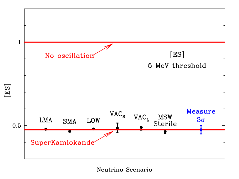
FIG. 6.: The reduced neutrino-electron scattering rate, [ES]. The figure shows the reduced neutrino-electron scattering rate [cf. Eq. (24)] from the standard model value of $1.0$ (no oscillations). The Super-Kamiokande result (see Ref. [3]) is also shown. The solid error bars represent the $99$% C.L. for the allowed regions of the six currently favored neutrino oscillation solutions [4]. The dashed error bar labeled “Measure $3\sigma$” represents the uncertainty in interpreting the measurements according to the estimates in Table III, which include the energy resolution, energy scale, ⁸B neutrino energy spectrum, neutrino cross section, counting statistics, and the $hep$ flux. The oscillation predictions are calculated assuming a $5$ MeV threshold for the total electron recoil energy.

VII The neutral current to charged current double ratio

In this section, we present predictions for the ratio of neutral current events (NC) to charged current events (CC) in SNO. The most convenient form in which to discuss this quantity is obtained by dividing the observed ratio by the ratio computed assumed the correctness of the standard electroweak model (SM). This double ratio is defined by the relation [10]

$${\rm{[NC]}\over{[CC]}}={{\left({\rm(NC)_{Obs}/(NC)_{SM}}\right)}\over{\left({\rm(CC)_{Obs}/(CC)_{SM}}\right)}}.$$ (25)

The ratio ${\rm{[NC]}/{[CC]}}$ is equal to unity if nothing happens to the neutrinos after they are produced in the center of the sun (no oscillations occur). Also, ${\rm{[NC]}/{[CC]}}$ is independent of all solar model considerations provided that only one neutrino source, ⁸B, contributes significantly to the measured rates. Finally, the calculational uncertainties due to the interaction cross sections and to the shape of the ⁸B neutrino energy spectrum are greatly reduced by forming the double ratio (see Table III).

Table VIII presents the calculated range of the double ratios for the oscillation solutions that are currently allowed at $99$% CL [4]. The table gives the best-fit values for ${\rm{[NC]}/{[CC]}}$ as well as the maximum and minimum allowed double ratios for a total electron energy threshold for the CC reaction of $5$ MeV and separately for a CC threshold of $8$ MeV.

TABLE VIII.: Neutral Current to Charged Current Double Ratio. The table presents the double ratio, ${\rm[NC]/[CC]}$, that is defined by Eq. (25). The results are tabulated for different neutrino oscillation scenarios and for two different thresholds of the total electron recoil energy used in computing the CC ratio, 5 MeV (columns two through four) and 8 MeV (columns five through seven).

$Scenario$	$[NC]/[CC]$	$[NC]/[CC]$	$[NC]/[CC]$	$[NC]/[CC]$	$[NC]/[CC]$	$[NC]/[CC]$
	b.f.	$max$	$min$	b.f.	$max$	$min$
	$5MeV$	$5MeV$	$5MeV$	$8MeV$	$8MeV$	$8MeV$
$LMA$	$3.37$	$5.15$	$2.27$	$3.36$	$5.13$	$2.30$
$SMA$	$2.53$	$4.11$	$1.24$	$2.28$	$3.50$	$1.21$
$LOW$	$2.71$	$3.39$	$2.30$	$2.69$	$3.35$	$2.26$
${\rm VAC_{S}}$	$2.67$	$4.63$	$1.37$	$2.33$	$3.73$	$1.27$
${\rm VAC_{L}}$	$1.90$	$2.15$	$1.53$	$2.01$	$2.45$	$1.53$
${\rm Sterile}$	$0.96$	$0.99$	$0.94$	$0.88$	$0.97$	$0.82$

Figure 7 compares the predicted values of [NC]/[CC] with the no-oscillation value of 1.0. The results are shown for a 5 MeV CC threshold and for an 8 MeV CC threshold. The estimated [see Eq. (27)] non-statistical errors are smaller than the black dots indicating the best-fit points in Fig. 7.

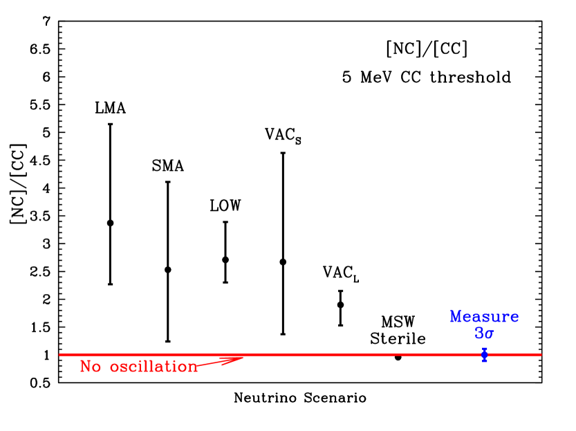
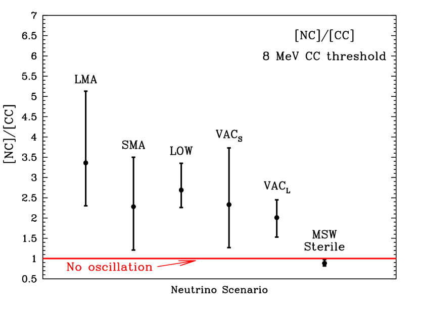
FIG. 7.: The neutral current to charged current double ratio. The double ratio, [NC]/[CC] is defined by Eq. (25). The standard model value for [NC]/[CC] is $1.0$. Figure 7a shows, for a 5 MeV threshold for the CC measurement, the predicted double ratio of Neutral Current to Charged Current for different neutrino scenarios. Figure 7b shows the same ratio but for an 8 MeV CC threshold. The solid error bars shown represent the $99$% C.L. for the allowed regions of the six currently favored neutrino oscillation solutions [4]. The dashed error bar labeled “Measure $3\sigma$” represents the uncertainty in interpreting the measurements according to the estimates in Table III, which include the energy resolution, energy scale, ⁸B neutrino energy spectrum, neutrino cross section, counting statistics, and the $hep$ flux.

The best-fit values for the double ratio for oscillations into active neutrinos range between $1.9$ and $3.4$ ($2.0$ and $3.4$) for a 5 MeV (8 MeV) CC threshold. The maximum predicted values for ${\rm{[NC]}/{[CC]}}$ exceed $5.1$. For active neutrino oscillations, the minimum values for the double ratio are achieved by the SMA and the ${\rm VAC_{L}}$ solutions; they are $1.2$ and $1.5$, respectively.

The sterile neutrino solutions predict a double ratio in a band that is separate from all the active oscillation solutions, namely, $0.9$ to $1.0$. The physical reason that the double ratio for sterile neutrinos is less than $1.0$ is that in the SMA solution (for active or sterile neutrinos) the probability that a solar $\nu_{e}$ survives as a $\nu_{e}$ decreases with energy (see, e.g., Fig.  9 of Ref. [6]). In the sterile neutrino case, if the $\nu_{e}$ oscillates to another state it does not interact. Since the NC threshold is $2.2$ MeV and the observational threshold for CC events is likely to be $5$ MeV or above, the smaller survival probability at low energies more strongly affects the average NC rate than the average CC rate.

The standard model value for ${\rm{[NC]}/{[CC]}}$ is

$${\rm{[NC]}\over{[CC]}} = 1.0~{}\pm 0.004^{\rm a}~{}\pm 0.003^{\rm b}~{}\pm 0.004^{\rm c}~{}\pm 0.015^{\rm d}~{}\pm 0.02^{\rm e}$$ (26)

$$= 1.0\pm 0.026.$$ (27)

The uncertainties, all non-statistical, shown in Eq. (27) result from: (a) the difference between the Ying, Haxton, and Henley [29] and Kubodera-Nozawa cross sections  [28], (b) the shape of the ⁸B neutrino energy spectrum [27], (c) the energy resolution function, (d) the absolute energy scale, and (e) the NC detection efficiency. Comparable, but small, contributions are made by the cross section uncertainties, the uncertainties in the shape of the neutrino energy spectrum, and the uncertainty in the energy resolution function. The absolute energy scale and the NC detection efficiency are expected to contribute even less to the errors.

One of the principal uncertainties in interpreting the electron recoil energy spectrum is the poorly known value for the flux of the extremely rare $hep$ neutrinos [35, 36]. The uncertainty in the $hep$ flux can also affect the otherwise robust measurement of ${\rm{[NC]}/{[CC]}}$ (see Table III). We have recalculated the value of ${\rm{[NC]}/{[CC]}}$ for a $hep$ flux that is $20$ times larger than the nominal standard model flux [5]. We find [cf. Eq. (8) for the calculational prescription]

$${\rm{[NC]}\over{[CC]}}~{}=~{}1.0-\epsilon_{hep}\left({\phi(hep)}\over{20\,\phi(hep,~{}{\rm BP98})}\right),$$ (28)

where $\epsilon_{hep}=0.0005$ for a 5 MeV threshold on the CC events and $0.017$ for an 8 MeV CC threshold. For an 5 MeV CC threshold, there is an accidental cancellation of the contributions to the neutral current ratio, [NC], and to the charged current ratio, [CC], so that the net value of $\epsilon_{hep}({\rm 5~{}MeV})$ is very small. But, for an 8 MeV threshold, the $hep$ flux causes an uncertainty, $1.7$%, that is larger than the combined contribution from all the other known uncertainties except possibly counting statistics [cf. Eq. (27) and Eq. (28) and Table III]. Of course, the gain at lower energies due to the reduction in the uncertainty from the $hep$ neutrinos may be more than offset by the increased uncertainty due to background events. Fortunately, SNO is expected to be able to measure or to place strong limits on the $hep$ flux within the first full year of operation [4].

We have not included the statistical uncertainties in the calculational error budget of Eq. (27). It seems likely that statistical errors will dominate over calculation errors, at least in the first several years of operation of SNO (see Table III). The CC rate may be in the range of 3000 to 4000 events per year. The NC event rate in the detector will be about a factor of two smaller and the NC detection rate will be further decreased by the NC detection efficiency that may be of order $50$%. Thus statistical errors in the NC rate, the uncertainty ($\sim 2$%, see Table III) in the NC detection rate, and the uncertainties in the $hep$ flux, will probably be the limiting factors in determining the accuracy of the experimental measurement of [NC]/[CC].

The small calculational error [see Eq. (27)] for ${\rm{[NC]}/{[CC]}}$, combined with the relatively large differences between the no-oscillation and the oscillation values for active neutrinos (Table VIII), makes the double ratio an ideal ‘smoking-gun’ indicator of oscillations.

VIII The Electron-scattering to CC Double Ratio

In this section, we present results for the double ratio of neutrino-electron scattering to CC events. This ratio is defined, by analogy with the NC to CC double ratio [see Eq. (25)], by the expression

$${\rm{[ES]}\over{[CC]}}={{\left({\rm(ES)_{Obs}/(ES)_{SM}}\right)}\over{\left({\rm(CC)_{Obs}/(CC)_{SM}}\right)}}.$$ (29)

The double ratio ${\rm{[ES]}/{[CC]}}$ has some of the same advantages as the double ratio ${\rm{[NC]}/{[CC]}}$, namely, independence of solar model considerations and partial cancellation of uncertainties. In fact, the ${\rm{[ES]}/{[CC]}}$ double ratio has the additional advantage that the same detection process is used for the recoil electrons from both the scattering and the CC reactions. For the ${\rm{[NC]}/{[CC]}}$ double ratio, different techniques are used to determine the two rates and this increases the systematic measurement uncertainty in the ratio.

TABLE IX.: Neutrino-Electron Scattering to Charged Current Double Ratio. The table presents the double ratio, ${\rm[ES]/[CC]}$, that is defined by Eq. (29). The results are tabulated for different neutrino oscillation scenarios and for two different thresholds of the total electron recoil energy for both the scattering and the CC reactions, 5 MeV (columns two through four) and 8 MeV (columns five through seven).

$Scenario$	$[ES/CC]$	$[ES/CC]$	$[ES/CC]$	$[ES/CC]$	$[ES/CC]$	$[ES/CC]$
	b.f.	$max$	$min$	b.f.	$max$	$min$
	$5MeV$	$5MeV$	$5MeV$	$8MeV$	$8MeV$	$8MeV$
$LMA$	$1.37$	$1.65$	$1.20$	$1.36$	$1.63$	$1.19$
$SMA$	$1.20$	$1.43$	$1.03$	$1.29$	$1.57$	$1.05$
$LOW$	$1.27$	$1.37$	$1.20$	$1.26$	$1.37$	$1.20$
${\rm VAC_{S}}$	$1.25$	$1.58$	$1.03$	$1.16$	$1.38$	$1.02$
${\rm VAC_{L}}$	$1.15$	$1.20$	$1.08$	$1.18$	$1.29$	$1.05$
${\rm Sterile}$	$0.96$	$0.99$	$0.92$	$1.06$	$1.08$	$1.02$

The standard model value for ${\rm{[ES]}/{[CC]}}$ is

$${\rm{[ES]}\over{[CC]}} = 1.0~{}\pm 0.06^{\rm a}~{}\pm 0.006^{\rm b}~{}\pm 0.003^{\rm c}~{}\pm 0.01^{\rm d}~{}$$ (30)

$$= 1.0\pm 0.06,$$ (31)

where the non-statistical uncertainties shown in Eq. (31) result from: (a) the difference between the Ying, Haxton, and Henley [29] and Kubodera-Nozawa cross sections  [28] neutrino cross sections, (b) the shape of the ⁸B neutrino energy spectrum [27], (c) the energy resolution function, and (d) the absolute energy scale. The upper limit $hep$ uncertainty is small, $0.007$ (see Table III).

The uncertainty in the double ratio [ES]/[CC] is dominated by the uncertainty in the CC absorption cross section and by statistical errors ($\sim 4.9$% after 5000 CC events, see Table III) that are not included in Eq. (31).

Table IX presents the calculated range of ${\rm{[ES]}/{[CC]}}$ for the oscillation solutions that are currently allowed at $99$% CL [4]. The table gives the best-fit values for ${\rm{[ES]}/{[CC]}}$ as well as the maximum and minimum allowed double ratios for a total electron energy threshold (for both reactions) of either $5$ MeV or $8$ MeV. The range of ratios predicted by oscillations into active neutrinos is $1.03$ to $1.65$, much smaller than the range ($1.24$ to $5.1$) predicted for the ${\rm{[NC]}/{[CC]}}$ double ratio.

Figure 8 shows the values of [ES]/[CC] predicted by the different oscillation solutions. Comparing Fig. 8 and Fig. 7, one can see that the neutral current to charged current ratio is a more sensitive diagnostic of neutrino oscillations than is the electron scattering to charged current ratio. The difference from the no-oscillation solution is much greater for the [NC]/[CC] double ratio than it is for the [ES]/[CC] double ratio. In addition, there are expected to be many more detected NC events than neutrino-electron scattering events. Also, the cross section uncertainties largely cancel out of the ratio ${\rm{[NC]}/{[CC]}}$, whereas the uncertainty in the CC cross section is an important limitation in interpreting the ratio [ES]/[CC].

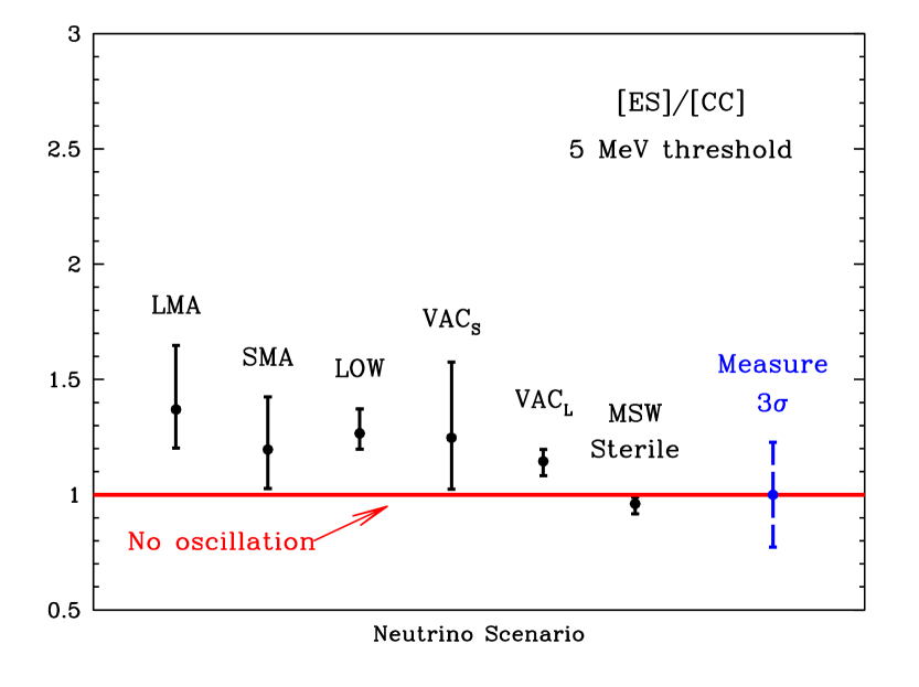
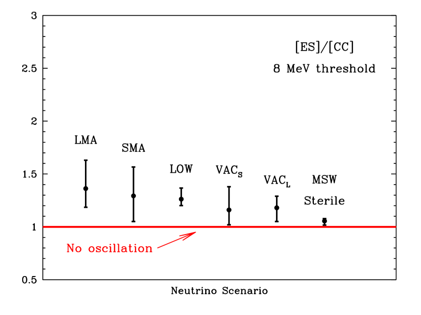
FIG. 8.: The neutrino-electron scattering to charged current double ratio. The double ratio, [ES]/[CC] is defined by Eq. (29). Figure 8a shows, for a 5 MeV electron recoil energy threshold, the predicted double ratio of Neutrino-Electron Scattering to Charged Current for different neutrino scenarios. The solid error bars represent the $99$% C.L. for the allowed regions of the six currently favored neutrino oscillation solutions [4]. The dashed error bar labeled “Measure $3\sigma$” represents the uncertainty in interpreting the measurements according to the estimates in Table III, which include the energy resolution, energy scale, ⁸B neutrino energy spectrum, neutrino cross section, counting statistics, and the $hep$ flux. Figure 7b shows the same ratio but for an 8 MeV threshold. Figure 8, which has a vertical scale extending from $0.5$ to $3.0$, should be compared with Fig. 7, which has a vertical scale extending from $0.5$ to $7.0$. The difference from the no-oscillation solution is much greater for the [NC]/[CC] double ratio than it is for the [ES]/[CC] double ratio.

IX The day-night effect

We discuss in this section the difference between the event rate observed at night and the event rate observed during the day. For MSW solutions, the interactions with matter of the earth can change the flavor content of the solar neutrino beam and cause the nighttime and daytime rates to differ. This effect has been discussed and evaluated by many different authors, including those listed in Ref. [42].

We concentrate here on the difference, $A_{\rm N-D}$, between the nighttime and the daytime rates, averaged over one year. The formal definition of $A_{\rm N-D}$ is

$$A_{\rm N-D}~{}=~{}2{\rm{[Night-Day]}\over{[Night+Day]}}.$$ (32)

In what follows, we shall use $A_{\rm N-D}$ to refer to the charged current reaction. When we want to consider the quantity defined by Eq. (32) for the neutral current, we shall write $A_{\rm N-D}({\rm NC})$.

We begin by discussing in Sec. IX A the apparent day-night effect that arises solely from the eccentricity of the earth’s orbit and the inclination of the earth’s axis (the existence of seasons), and then we discuss in Sec. IX B the day-night effect for the CC reaction and in Sec. IX C the day-night effect for the NC reaction due to oscillations.

A The No-Oscillation day-night effect

In the absence of neutrino oscillations, there is a geometrical day-night effect that we have not seen discussed in previous publications. This No-Oscillation (NO) effect is caused by the ellipticity of the earth’s orbit and by the fact that, in the northern hemisphere, nights are longer (days are shorter) in winter when the earth is closer to the sun. Thus the average over the year of the nighttime rate will be larger than the annual average of the daytime rate for all detectors located in the northern hemisphere.

We find that the No-Oscillation (NO) day-night effect is

$$A^{\rm No}_{\rm N-D} ~{}=~{} 0.0094~{}~{}({\rm SNO}),$$ (33)

$$A^{\rm No}_{\rm N-D} ~{}=~{}~{} 0.0066~{}~{}({\rm SK}),$$ (34)

$$A^{\rm No}_{\rm N-D} ~{}=~{} 0.0082~{}~{}({\rm Gran~{}Sasso}),$$ (35)

$$A^{\rm No}_{\rm N-D} ~{}=~{} 0.0088~{}~{}({\rm Homestake}),$$ (36)

for the locations of the SNO, Super-Kamiokande, Gran Sasso, and Homestake detectors.

The No-Oscillation effect is purely geometrical; it is independent of neutrino energy and independent of neutrino flavor. The magnitude of the NO effect is the same for the CC, ES, and NC reactions. The numerical results given in Eq. (34)– Eq. (36) can also be obtained from the following easily-derived relation, which makes clear the seasonal aspect of the NO effect:

$$A^{\rm No~{}Osc.}_{\rm N-D}\approx 2\epsilon{{\left(t_{\rm max}-t_{\rm min}\right)}\over{24}},$$ (37)

where $\epsilon=0.0167$ is the eccentricity of the earth’s orbit and $t_{\rm max}$ and $t_{\rm min}$ are, respectively, the length of the longest and the shortest nights in the year at the location of the detector.

In what follows, we remove the No-Oscillation day-night effect before presenting the predictions of an additional day-night effect that is due to neutrino oscillations. More precisely, we calculate the day-night effect assuming that the neutrino flux from the sun is constant throughout the year. The effects that we discuss in Sec. IX B and in Sec. IX C are due to neutrino mixing.

Experimental results can easily be analyzed so as to remove the NO day-night effect. All that is required is to multiply the number of events in each time bin ($\Delta t\ll$ 1 year) by the ratio $\left[r(t)/(1~{}{\rm A.U.})\right]^{2}$, where $r(t)$ is the average earth-sun distance in that time bin and 1 A.U. is the annual average earth-sun distance. This is the procedure adopted by the Super-Kamiokande collaboration [3].

Even after these corrections, there is a residual day-night effect for vacuum oscillations. In this case, the day-night effect is due to the variation of the survival probability as a function of the distance between the earth and the sun and the fact that in the northern hemisphere the longest nights occur when the earth is closest to the sun. We are not aware of any previous discussions of the day-night effect for vacuum oscillations. For MSW oscillations, the day-night effect is caused by neutrino flavor changes during propagation in the earth.

B The CC day-night effect

Table X and Fig. 9 present the range of predicted percentage differences between the average rate at night and the average rate during the day [i.e., $100\times A_{\rm N-D}$ of Eq. (32)]. The calculated predictions are given for a $5$ MeV and an $8$ MeV CC electron recoil energy threshold.

For vacuum oscillations, the day-night effect is due to the dependence of the survival probability upon the earth-sun distance. The predicted day-night effect for vacuum oscillations is small in all the cases shown in Table X and in Fig. 9.

For most of the MSW oscillation solutions, the predicted day-night differences are only of order a few percent. However, for the LMA solution, the predicted difference can reach as high as $29$% for a $5$ MeV threshold ($32$% for an $8$ MeV threshold). There are also rather large differences, in excess of $10$%, that are possible for the SMA and LOW solutions.

At first glance, one might think that such large day-night differences will be easy to measure. In fact, there are important systematic uncertainties that have to be taken into account in making sure that the relative sensitivities to the day and the night rates are properly evaluated [3]. Even the purely statistical uncertainties are very significant because the day-night difference, $A_{\rm N-D}$, is the difference between two comparably sized large numbers. Thus the fractional statistical uncertainty after accumulating a large number, $N$, of counts at night (and a roughly equal number during the day) is

$${\sigma(A_{\rm N-D})\over A_{\rm N-D}}~{}\simeq~{}\left({1\over A_{\rm N-D}}\right){\sqrt{2\over N}}.$$ (38)

The fact that $A_{\rm N-D}$ can be a small number makes a multi-sigma statistical measurement of the day-night effect difficult. The careful analysis of the day-night effect by the Super-Kamiokande collaboration [3] has demonstrated the practical difficulty of a precision measurement of $A_{\rm N-D}$. Using more than $800$ effective days of operation of the SuperK detector with total night time counts of $N\sim 5900$ ($\sim 11,200$ total events) the precision obtained by the Super-Kamiokande collaboration is $A_{\rm SK}~{}=~{}0.065\pm 0.03$, i.e., $\Delta A/A\sim 0.5$. To accumulate with SNO an equivalent number of CC events ($\sim 11,000$ total events) may require of order three years or longer of operation.

TABLE X.: The Predicted Night-Day Difference (in %) for the CC Rate. The table gives the percentage difference in the Night-Day CC rates, $A_{\rm N-D}$, defined by Eq. (32). For a $5$ MeV ($8$ MeV) threshold energy for recoil electrons, the second (fifth) column gives the best-fit value, and the third (sixth) and fourth (seventh) columns give the minimum and maximum values, allowed at 99% CL for different neutrino oscillation solutions (cf. Fig. 1 of Ref. [4]).

Scenario	b.f.	$min$	$max$	b.f.	$min$	$max$
LMA	$12.4$	$+0.5$	$28.5$	$14.1$	$0.7$	$31.6$
SMA	$1.6$	$-1.1$	$12.3$	$1.2$	$-1.3$	$10.9$
LOW	$4.7$	$+1.1$	$13.5$	$4.0$	$0.8$	$11.8$
${\rm VAC_{S}}$	$0.5$	$-0.1$	$1.0$	$0.7$	$0.2$	$1.2$
${\rm VAC_{L}}$	$0.3$	$-0.1$	$0.5$	$1.0$	$-0.1$	$1.5$
MSW, Sterile	$-0.1$	$-0.4$	$1.1$	$-0.2$	$-0.7$	$1.1$

Why is the predicted effect in SNO (see also Ref. [43]) so much larger than for Super-Kamiokande? The reason is that for neutrino-electron scattering the day-night effect is decreased relative to the pure CC mode by the contribution of the neutral currents. For the LMA solution, one can derive a simple quantitative relation between the CC day-night effect, $A^{\rm CC}$, and the ES day-night effect, $A^{\rm ES}$. Let the nighttime rate be proportional to $P_{\rm N}+r(1-P_{\rm N})$, where $P_{\rm N}$ is the average (over energy) survival probability during the night and $r$ is the average ratio of $\nu_{\mu}-e$ to $\nu_{e}-e$ scattering cross sections. Writing a similar expression for the daytime rate, it is easy to show that

$$A^{\rm CC}_{\rm N-D}~{}=~{}A^{\rm ES}_{\rm N-D}\left[1+{{r}\over{(1-r)P}}\right],$$ (39)

where $P$ is the average of the day and the night survival probabilities. Since $r\approx 0.16$ and $P\approx 0.3$ for the best-fit solution, we see that the term in brackets in Eq. (39) is about $1.6$. For the LMA solution, the best-fit predicted value for $A^{\rm SK}$ is $8$% for a $5$ MeV recoil energy threshold, which corresponds to about $13$% for SNO, in good agreement with the value of $12.5$% given in Table X. There are small corrections to Eq.( 39) due to the energy dependence of the various neutrino quantities (and the different locations on the earth of the SNO and the Super-Kamiokande detectors).

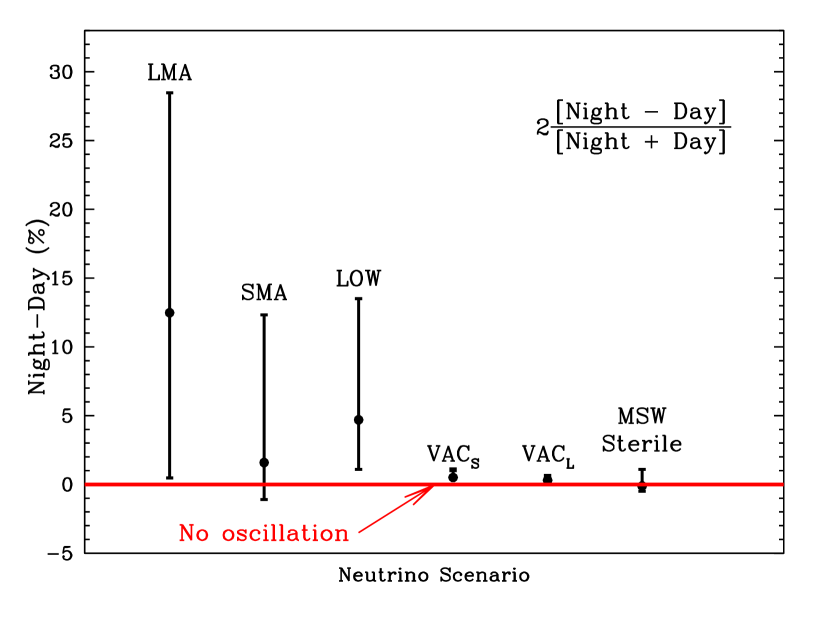
FIG. 9.: The percentage difference between the night and the day CC rates. The figure shows for different neutrino scenarios the percentage difference between the predicted CC rate in SNO at night and the CC rate in the day [see Eq. (32)]. The error bars represent the $99$% C.L. for the allowed regions of the six currently favored neutrino oscillation solutions [4]. The results were calculated with a CC threshold of 5 MeV for the total electron recoil energy.

C The NC day-night effect

There is no day-night effect in the NC for oscillations into active neutrinos. All active neutrinos are recorded with equal probability by the neutral current detectors. However, for oscillations into sterile neutrinos there can be a day-night effect since the daughter (sterile) neutrinos are not detectable. Thus a day-night effect in the NC would be a ‘smoking gun’ indication of sterile neutrino oscillations.

For the region that is allowed at $99$% CL by a global fit of the MSW sterile neutrino solution to all the available neutrino data [4], we find a NC MSW sterile neutrino day-night effect of

$$A({\rm NC,~{}MSW~{}Sterile})~{}=~{}-0.001^{+0.006}_{-0.002}.$$ (40)

Although the predicted effect is small, it is important in principle since there are very few ways that sterile neutrino oscillations can be identified uniquely [26].

The neutral current day-night effect for solar neutrinos was first pointed out in Ref. [44]. Here we have calculated accurately the predicted range of the day-night asymmetry given the latest solar neutrino data, solar model, and a realistic model of the earth.

X Seasonal effects

We discuss in this section the seasonal dependences that are predicted by the currently favored neutrino oscillation solutions. We define a Winter-Summer Asymmetry by analogue with the Night-Day difference. Thus

$$A_{\rm W-S}~{}=~{}2{\rm{[Winter-Summer]}\over{[Winter+Summer]}}.$$ (41)

The earth’s motion around the sun causes a seasonal dependence that can be calculated and is

$$A_{\rm W-S,~{}orbital}=0.064~{}~{}({\rm 45~{}day~{}averages})$$ (42)

for a 45 day Winter interval centered around December 21 and a $45$ day Summer interval centered around June 21. The average length of the winter (summer) night during this $45$ day period is $15.4$ ($8.5$) hours. The amplitude is reduced if the entire year is divided into two parts, with the winter average being taken as $182$ days centered on December 21 and with the average length of the winter (summer) night being $14.1$ ($9.7$) hours. In this case, the asymmetry is reduced by a factor of $1.5$ from the $45$-day value. Thus

$$A_{\rm W-S,~{}orbital}=0.042~{}~{}({\rm 182~{}day~{}averages}).$$ (43)

In what follows, we have removed the seasonal dependence due to the orbital motion from the quoted values of the seasonal dependence due to neutrino oscillation effects.

FIG. 10.: The seasonal dependence of the CC event rate in SNO. The figure shows the dependence on the time of the year of the predicted CC event rate in SNO for the six best-fit neutrino oscillation solutions described in Table I. The time labeled zero on the horizontal axis corresponds to January 1.

Figure 10 shows the predicted dependence upon the day of the year of the CC event rate, $R_{\rm cc}$, in SNO for each of the currently favored best-fit oscillation solutions. The vertical scales are different, reflecting the fact that the predicted seasonal variations are, e.g., relatively large for the best-fit LMA and ${\rm VAC_{L}}$ solutions, but are tiny for the MSW sterile solution. The annual average of the events rates shown in Fig. 10 yields the numbers shown in the second column of Table VI. The alert reader may notice that the phases of the variations in the two panels referring to vacuum oscillations are shifted by about two weeks with respect to the four panels that refer to MSW oscillations. This shift results from the fact that the earth and the sun are closest (relevant for vacuum oscillations) on January 4 and the day with the longest night is December 21 (relevant for MSW oscillations).

Table XI and Fig. 11 show the calculated percentage amplitudes for the 45 day winter-summer difference due to oscillations, $A_{\rm W-S}$. In all cases, the best-fit oscillation solutions predict a winter-summer difference due to neutrino properties that is less than the orbital effects given in Eq. (42) and Eq. (43). Only rather extreme cases give amplitudes of $A_{\rm W-S}$ due to oscillations that are as large as the orbital amplitude, which will itself require a number of years to establish definitively [1].

TABLE XI.: The Winter-Summer Predicted Difference in the CC Rate. The table gives the percentage difference, $A_{\rm W-S}$, in the Winter-Summer CC rates, defined by Eq. (41). The results on the first row for each oscillation solutions have been computed for $45$ days in winter and $45$ days in the summer; the results on the second row are average over $182$ days of winter and $182$ days of summer. The second column gives the best-fit value, and the third and four columns give the minimum and maximum values, allowed at 99% CL for different neutrino oscillation solutions (cf. Fig. 1 of Ref. [4]). The winter-summer asymmetry due to the earth’s motion around the sun, $A_{\rm W-S,~{}orbital}=6.4\%(4.2\%)$ for a $45$ day ($182$ day) average, has been removed from the values given here.

Scenario	b.f.	$min$	$max$
Interval	$45d$	$45d$	$45d$
	$182d$	$182d$	$182d$
LMA	$3.6$	$0.2$	$7.7$
	$2.4$	$0.1$	$4.7$
SMA	$1.9$	$-0.9$	$11.8$
	$1.1$	$-0.7$	$7.8$
LOW	$1.0$	$0.25$	$2.9$
	$0.6$	$0.15$	$1.7$
${\rm VAC_{S}}$	$3.4$	$-0.9$	$6.9$
	$2.2$	$-0.6$	$4.5$
${\rm VAC_{L}}$	$2.0$	$-0.6$	$3.6$
	$1.3$	$-0.4$	$2.4$
MSW, Sterile	$-0.1$	$-0.55$	$1.1$
	$-0.1$	$-0.3$	$0.55$

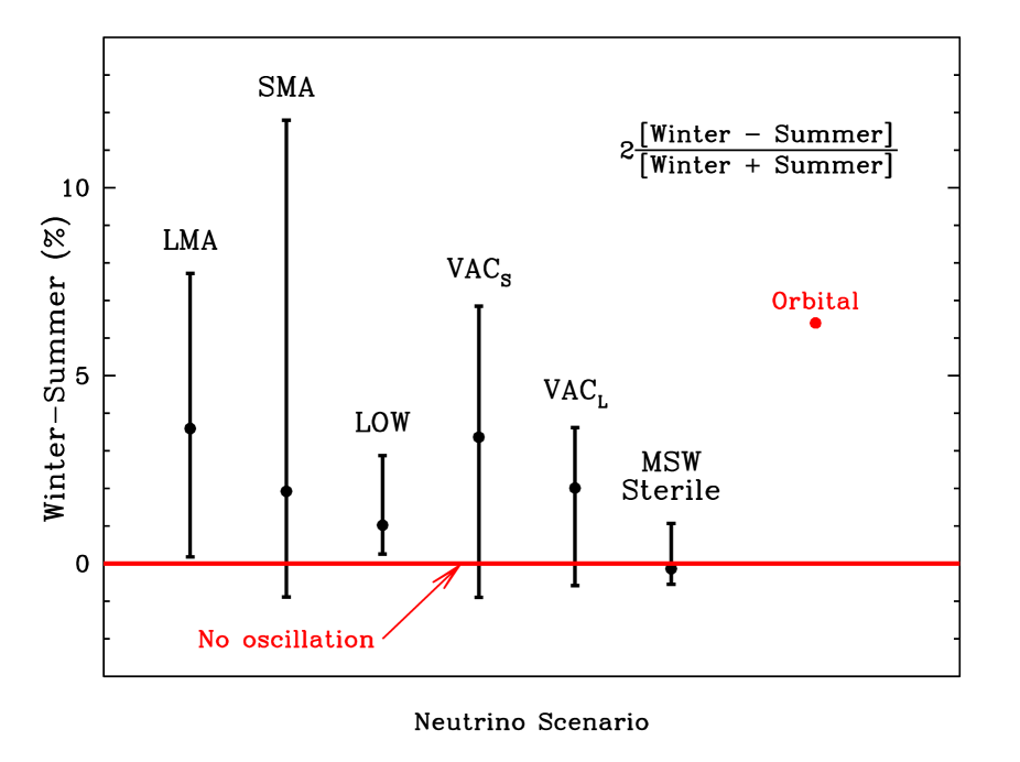
FIG. 11.: The difference between the winter and the summer rates. The figure shows for different neutrino scenarios the percentage difference between the predicted CC rate in SNO for a 45 day interval during winter and the CC rate for a 45 day interval in the summer [see Eq. (41)]. The point labeled ‘Orbital’ represents the 45 day winter-summer difference due to the earth’s motion around the sun; the amplitude of this orbital motion has been removed from the neutrino oscillation points. The error bars represent the $99$% C.L. for the allowed regions of the six currently favored neutrino oscillation solutions [4]. The results were calculated with a CC threshold of 5 MeV for the total electron recoil energy.

Table XI also gives the predicted values of $A_{\rm W-S}$ for a longer average, $182$ of winter and $182$ of summer. For this case the statistical error will be reduced by about a factor of two, but the size of the effect is typically reduced by a factor of order $1.5$ to $1.7$.

For the LMA solution, we showed in Ref. [45] that to a good approximation $A_{\rm W-S}$ and $A_{\rm N-D}$ are related by the equation

$$A_{\rm W-S}=A_{\rm N-D}\left[\frac{t_{W}-t_{S}}{24~{}{\rm h}}\right],$$ (44)

where $t_{W}$ and $t_{S}$ are the average lengths of the nights during the selected winter and summer periods, respectively. For the $45$ day ($182$ day) intervals we are discussing here, the length at SNO of the winter night is $15.43$ hours ($14.10$ hours) and the length of the summer night is $8.49$ hours ($9.72$ hours). The term in brackets in Eq. (44) is $1.6$ times larger for the $45$ day period (longer nights) than for the $182$ day period. This accounts well for the ratios of $A_{\rm W-S}$ for the $45$ day and the $182$ periods that are given in Table XI . Eq. (44) also produces well the individual values of $A_{\rm W-S}$ for the LMA solution. Using the best-fit value of $A_{\rm N-D}=12.48$% (from Table X) and $(t_{W}-t_{S})/(24~{}{\rm h})=0.29$, we estimate $A_{\rm W-S}=3.6$% for the $45$ day average, in good agreement with the result given in Table XI.

From the size of the predicted effects shown in Table XI and Fig. 11, we conclude that it will require many years of SNO operation to measure an accurate value of $A_{\rm W-S}$ if the currently favored oscillation solutions are correct.

XI Smoking gun vs. smoking gun

What do we gain by combining the measurements of different smoking gun quantities? Once SNO has begun to report results for a variety of different quantities and an accurate Monte Carlo of the experimental facility exists, then it will be possible to analyze simultaneously a variety of different measurements using a global analysis method like Maximum Likelihood. In the meantime, we begin an initial illustrative exploration by analyzing pairs of SNO measurements.

We show in this section how comparisons of the measurements of different smoking-gun quantities versus each other can enhance the deviation of a single measurement from the no-oscillation expectation and also shrink the globally-allowed range of the oscillation parameters. We concentrate on the most powerful pairwise combinations of variables. We do not illustrate all possible combinations, omitting some examples (like day-night effect versus first moment of the CC energy spectrum) that turn out to be less useful when examined quantitatively.

We begin by displaying and discussing in Sec. XI A the predicted oscillation regions in planes defined by the double ratio [NC]/[CC] versus either 1) the day-night effect, $A$; 2) the first moment, $\langle T\rangle$, of the CC recoil energy spectrum; and 3) the neutrino-electron scattering reduced rate, [ES]. The double ratios involving the neutral current discriminate sharply between oscillation and no-oscillation scenarios and also reduce the range of acceptable oscillation parameters. In Sec. XI B and Sec. XI C, we discuss the location of the favored oscillation solutions in the [ES]/[CC] versus $\langle T\rangle$ plane and in the plane of the CC rate, $R_{\rm CC}$ versus the first moment, $\langle T\rangle$.

For each plane defined by two SNO parameters and for each of the six neutrino oscillation solutions, we plot error bars that represent separately the $99$% C.L. acceptable range of the neutrino parameters in the global fits to all the currently available solar neutrino data [4]. The $1\sigma$ experimental uncertainties are summarized in Table III. The statistical uncertainties are computed assuming $5000$ CC events, $1219$ NC events, and $458$ ES events. We assume that the $hep$ uncertainties are symmetric and equal to the upper limit uncertainty, which slightly increases the error contours. For the no-oscillation case, only the experimental measurements are correlated. When neutrino oscillations occur, the predicted values for different parameters are also correlated. We include here only the correlations of the uncertainties for the no-oscillation case; we do not include the correlated contours for the six different predicted oscillation solutions. A full calculation that includes the theoretical correlations between the different measured parameters and also includes asymmetric $hep$ uncertainties should be carried out in the future, but this study is beyond the scope of the present paper.

The correlations between different estimated experimental uncertainties cause the no-oscillation error ellipses to be tilted in Fig. 12–Fig. 16. For purposes of illustration, we have assumed that the error correlations are as estimated in Ref. [11]. As we shall see from Fig. 12–Fig. 16, the tilt of the error ellipses can significantly influence the total statistical C.L. assigned to a given set of results and therefore accurate determinations of the error correlations for the SNO experiment will be important.

A [NC]/[CC] double ratio versus other smoking guns

1 [NC]/[CC] versus the day-night effect

Figure 12 shows the values predicted by the different oscillation solutions in the plane of the ${\rm[NC]/[CC]}$ double ratio and the day-night asymmetry, $A_{\rm N-D}$. Specifically, we plot the fractional shift in percent of the [NC]/[CC] double ratio from the standard model value of $0$% on the vertical axis and the predicted value in percent of the day-night asymmetry $A_{\rm N-D}$ (standard model value of $0$%) on the horizontal plane. Each of the currently allowed solutions, with the exception of the MSW Sterile solution, predicts points in the $\delta{\rm[NC]/[CC]}$–$A_{\rm N-D}$ plane that are more than $5\sigma$ separated from the standard model solution (which is located at $0\%,0\%$). Moreover, the vacuum solutions are separated from the MSW solutions by amounts that exceed the expected measuring errors in $A_{\rm N-D}$ and [NC]/[CC]. It will, however, be more difficult to distinguish between different MSW solutions in the $\delta{\rm[NC]/[CC]}$-$A_{\rm N-D}$ plane, although some measured values would point to a unique solution. For example, a large positive value of $A_{\rm N-D}$ ($\geq 20$%) combined with a large value of [NC]/[CC] ($\geq 2.3$) would favor the LMA solution. The allowed region for the MSW Sterile solution is all contained within the ellipse corresponding to the estimated $3\sigma$ experimental uncertainty.

FIG. 12.: The [NC]/[CC] double ratio versus the day-night asymmetry. The figure shows the fractional difference in percent of the neutral current versus charged current double ratio, [NC]/[CC] (Eq. 25), from the no-oscillation value of $1.0$, versus the day-night difference, $A_{\rm N-D}$ (Eq. 32)in percent. The standard model value of $A_{\rm N-D}$ is $0.0$. For the six currently preferred oscillation solutions, the error bars represent the $99$% C.L. regions for acceptable fits to all the available neutrino data. Estimated error contours for SNO are shown at the $1\sigma,2\sigma,3\sigma$, and $5\sigma$ levels relative to the no-oscillation solution which lies at $(0,0)$.

2 [NC]/[CC] versus $\langle T\rangle$

Figure 13 shows the predictions of the different oscillation solutions in the $\delta{\rm[NC]/[CC]}$ versus $\delta T$ plane. All of the currently favored oscillation solutions, with the exception of the MSW sterile solution, predict locations in the $\delta{\rm[NC]/[CC]}$ versus $\delta T$ plane that are separated by more than $5\sigma$ from the standard model solution, which lies at ($0.0,0.0$). However, the discrimination is almost entirely due to the [NC]/[CC] double ratio. The value of $\delta T$ only adds a large discrimination for the extreme ${\rm VAC_{S}}$ solution. The predicted values for the MSW Sterile solution extend out to $2.9$%, which because of the correlation of the experimental errors (which gives rise to the tilt of the error ellipses in Fig. 13), can correspond to deviations as large as $3\sigma$ from the no-oscillation solution.

FIG. 13.: The [NC]/[CC] double ratio versus the average recoil energy. The figure shows the fractional difference in percent of the neutral current versus charged current double ratio, [NC]/[CC] [Eq. (25)], from the no-oscillation value of $1.0$, versus the fractional difference in percent of the average electron recoil energy, $\langle T\rangle$ [Eq. (15)] , from the no-oscillation value [Eq. (14)]. Contours at $1\sigma,2\sigma,3\sigma$, and $5\sigma$ are shown relative to the no-oscillation solution at $(0,0)$.

3 [NC]/[CC] versus [ES]

The most likely value for SNO to observe for the neutrino-electron scattering ratio [ES] is close to the Super-Kamiokande [3] value of ${\rm[ES}_{SK}]=0.475$ (see for example Table VII or Fig. 6). It is therefore convenient to define the quantity $\delta({\rm[ES]})$ as follows:

$$\delta\left({\rm ES}\right)~{}\equiv~{}\frac{{\rm[ES]_{OBS}-0.475}}{{0.475}}.$$ (45)

We have used parentheses rather than squared brackets in defining $\delta\left({\rm ES}\right)$ because the shift in [ES] is measured relative to $0.475$ rather than $1.0$ .

Figure 14 shows the predictions of the different oscillation solutions in the $\delta{\rm[NC]/[CC]}$ versus $\delta{\rm(ES)}$ plane. Just as for Fig. 12 and Fig. 13, all of the currently favored oscillation solutions, with the exception of the MSW Sterile solution, are well separated (more than $5\sigma$ away) from the standard model solution, which lies at ($0.0,0.0$). For some of the ${\rm VAC_{S}}$ solutions, the predicted large positive value of $\delta{\rm[ES]}$ is incompatible with, and hence distinguishable from, the predictions of the other currently allowed solutions. This discrimination is a result of combining the values of both [NC]/[CC] and [ES] since the measurement of either of these parameters by itself would not permit, according to Fig. 14, the isolation of these ${\rm VAC_{S}}$ solutions.

!t

FIG. 14.: The [NC]/[CC] double ratio versus the neutrino-electron scattering double ratio. The figure shows the fractional difference in percent of the neutral current versus charged current double ratio, [NC]/[CC], from the no oscillation value of $1.0$, versus the fractional shift in percent of the reduced neutrino-electron scattering ratio from the Super-Kamiokande value of $0.475$ [see Eq. (45)]. Contours at $1\sigma,2\sigma,3\sigma$, and $5\sigma$ are shown relative to the no-oscillation solution at $(0,0)$.

B Electron-scattering and CC double ratio versus CC energy spectrum

Figure 15 shows the predictions of the different oscillation solutions in the $\delta{\rm[ES]/[CC]}$ versus $\delta T$ plane. Although there are some predictions that extend well beyond the $5\sigma$ contour in Fig. 15, these outlying predictions occur mostly for large values of [ES]/[CC] and should show up directly by comparing the neutrino-electron scattering rate with the CC (neutrino absorption) rate (see the discussion in Ref. [4]). The additional measurement of the first moment of the CC distribution, $\langle T\rangle$, does not add much to the discriminatory power of [ES]/[CC].

!t

FIG. 15.: The [ES]/[CC] double ratio versus the average CC electron recoil energy. The figure shows the fractional difference in percent of the electron-scattering-CC double ratio, [ES]/[CC], from the no-oscillation solution of $[ES]/[CC]=1.0$, versus the fractional shift in percent of the average electron recoil energy, $\langle T\rangle$ (Sec. III), from the no-oscillation value of Eq. (14). Contours at $1\sigma,2\sigma,3\sigma$, and $5\sigma$ are shown relative to the no-oscillation solution at $(0,0)$.

C CC rate versus CC energy spectrum

Figure 16 displays the six currently favored oscillation solutions in the plane of the CC rate, $R_{\rm CC}$, and the first moment of the CC electron-recoil energy spectrum, $\langle T\rangle$. Some of the currently allowed ${\rm VAC_{S}}$, SMA, and LMA solutions lie in this plane more than $5\sigma$ from the no-oscillation position. However, there are also currently allowed oscillation solutions that fall considerably closer to the no-oscillation point at ($0.0,0.0$).

!t

FIG. 16.: The CC rate versus the average recoil energy, $\langle T\rangle$. The figure shows the percent difference of the CC double rate, $R_{\rm cc}$, discussed extensively in Ref. [4], from the no-oscillation solution of $R_{\rm cc}=0.475$, versus the fractional difference [see Eq. (15)] of the average electron recoil energy, $\langle T\rangle$, from the no-oscillation value of Eq. (14). Contours at $1\sigma,2\sigma,3\sigma$, and $5\sigma$ are shown relative to the no-oscillation solution at $(0,0)$.

XII Summary and Discussion

We concentrate in this section on describing the results for the predictions of the six currently favored neutrino oscillation solutions that are globally consistent at the $99$% C.L. with all of the available neutrino data. The neutrino solutions are described in Table I and Fig. 1.

We begin this section by summarizing the results for parameters for which the estimated uncertainties are relatively small: 1) the neutral-current over charged current double ratio, Sec. XII A; 2) the shape of the CC electron recoil energy spectrum, Sec. XII B; 3) the day-night difference for the CC and for the NC, Sec. XII C; and 4) seasonal effects, Sec. XII D. Altogether, we discuss six measurable quantities in Sec. XII A–Sec. XII D.

We summarize the principal uncertainties, theoretical and experimental, in Sec. XII E. The uncertainties due to the $hep$ flux and the neutrino interaction cross sections are emphasized in this section; the estimates of the experimental uncertainties are very preliminary.

We then describe the predicted values and the potential inferences from SNO measurements for the CC rate, Sec. XII F, for the NC rate, Sec. XII G, and for the neutrino-electron scattering rate, Sec. XII H. Next we discuss in Sec. XII I the neutrino-electron scattering to CC double ratio, which has some of the same advantages as the neutral-current to charged current double ratio, but suffers from a relatively large uncertainty in the CC interaction cross section. Finally we summarize in Sec. XII J our initial exploration of combining the analysis of different smoking gun indicators of neutrino oscillations.

A Neutral current over charged current double ratio: [NC]/[CC]

All five of the currently favored oscillation solutions with active neutrinos predict that the double ratio, [NC]/[CC], will be separated from the no-oscillation value of $1.0$ by more than $9\sigma$, estimated non-statistical errors. The uncertainties due to the cross sections and to the solar model almost cancel out of the double ratio. The minimum predicted value for [NC]/[CC] is $1.24$ and the maximum predicted value is $5.15$, all for a $5$ MeV CC threshold. The estimated $1\sigma$ total non-statistical error is only $\pm 0.026$; the statistical error will be the largest uncertainty unless more than $5.5\times 10^{3}$ NC events are detected. The sterile neutrino solution lies in a disjoint region of [NC]/[CC] from $0.92$ to $0.99$.

The results are summarized in Fig. 7 and are given in more detail, for two different thresholds of the CC electron recoil energy, in Table VIII of Sec. VII.

The double ratio [NC]/[CC] is an ideal smoking gun indicator of oscillations into active neutrinos.

B The shape of the CC electron recoil energy spectrum: $\langle T\rangle$ and $\sigma(T)$

The shape of the CC electron recoil energy spectrum can be characterized by the first moment, $\langle T\rangle$, and the standard deviation, $\sigma(T)$, of the electron kinetic energy, $T$. With precision measurements of the spectrum, special features of the recoil energy spectra may also be detectable (cf. Fig. 4).

If there are no oscillations, the first moment is $\langle T\rangle_{0}=7.422\times(1\pm 0.013)~{}{\rm MeV}$, where the estimated uncertainty includes both the measurement and the calculational uncertainties. The best-estimate predictions for the different oscillation solutions correspond to a fractional shift between $0.1$% (LMA and LOW solutions) to $3.7$% (${\rm VAC_{S}}$ solution). The largest predicted value of the shift is $7.5$% (${\rm VAC_{S}}$ solution). The shift in the first moment may be measurable for the SMA, ${\rm VAC_{S}}$, ${\rm VAC_{L}}$, and MSW sterile neutrinos, but will be too small for a definitive measurement if the LMA or LOW solutions are correct. On the other hand, only the ${\rm VAC_{S}}$ solutions predict that the measured deviation of $\langle T\rangle$ from $\langle T\rangle_{0}$ will exceed three standard deviations for as much as half of the currently allowed solution space.

Figure 5 and Table IV (of Sec. III) show the predicted range of shifts in the first moment, $\langle T\rangle$, of the recoil energy spectrum. A measurement of $\langle T\rangle$ to a $1\sigma$ accuracy of $\sim 100$ keV will significantly reduce the allowed solution space for neutrino oscillations, but may not uniquely favor one particular solution.

The calculated no-oscillation value of the standard deviation of the CC recoil energy spectrum is $\sigma_{0}=\langle\sigma^{2}\rangle^{1/2}_{0}=1.852(1\pm 0.049)$ MeV. It will be difficult to measure the predicted shifts from $\sigma_{0}$ since the total spread in shifts given in Table V is from $-29$ keV to $199$ keV, while the estimated calculational and non-statistical measurement uncertainties are $\pm 86$ keV.

C Day-night difference: $A_{\bf N-D}$ and $A_{\rm N-D}({\rm NC})$

In the absence of neutrino oscillations, there is a purely geometrical day-night difference that we have defined as the No Oscillation (NO) effect and whose value for the SNO detector we have given in Eq. (33). We have removed the NO effect from all of the calculated day-night values given in this paper.

For the currently favored MSW active neutrino solutions, the best-fit predictions for the average difference between the nighttime and the daytime CC rates, $A_{\rm N-D}$, vary from $2$% for the SMA solution to $12.5$% for the LMA solution, all for a $5$ MeV recoil electron energy threshold. Small values ($<1$%) of the day-night difference would be consistent with any of the three MSW solutions, but very large values of the day-night difference are only expected for some of the LMA solutions. The maximum expected difference for the most extreme LMA solution is $28.5$%, whereas the maximum difference expected for the LOW (SMA) solution is $13.5$% ($12$%). The MSW sterile solution predicts values for the day-night asymmetry between $-0.5$% and $+1.1$%. Table X presents similar results also for an $8$ MeV electron recoil energy threshold.

For vacuum oscillations, the predicted values of the day-night effect are small, but non-zero (see Table X).

Initially, the dominant uncertainty for the day-night effect will be purely statistical. The most difficult problems will ultimately arise from systematic effects, such as the symmetry of the detector and the separation of the CC events from NC and scattering events, that will have to be modeled by a detailed SNO Monte Carlo simulation. The purely statistical error may be of order $4$% after one full year of operation. Whether or not the systematic errors affect in an important way the measurement of the day-night effect will depend upon the actual magnitude of $A_{\rm N-D}$ and the size of the systematic uncertainties.

Figure 9 and Table X present the numerical results for the CC day-night asymmetry which is defined by Eq. (32) of Sec. IX. If one of the MSW active neutrino solutions is correct, then the day-night difference could become apparent early in the operation of SNO. This possibility exists for the MSW active solutions, but is not required.

There is no day-night effect in the NC for oscillations into active neutrinos. Oscillations into sterile neutrinos give a small effect: $A_{\rm N-D}({\rm NC,~{}MSW~{}Sterile})~{}=~{}-0.001^{+0.006}_{-0.002}$ [see Eq. (40)]. This effect is important in principle, since it is a clear distinction between active neutrinos and sterile neutrinos. However, the predicted size is too small to be measured with SNO.

All of the currently favored neutrino oscillation solutions (MSW or vacuum oscillations into active neutrinos, as well as MSW oscillations into sterile neutrinos), predict that

$$\mid A_{\rm N-D}({\rm NC})\mid~{}<~{}0.01.$$ (46)

We have written Eq. (46) in its most general form. Of course, $A_{\rm N-D}({\rm NC})$ is predicted to be identically zero for all neutrino oscillations (vacuum or MSW) into active neutrinos.

The measurement by SNO of $A_{\rm N-D}({\rm NC})$ will be an important test of neutrino oscillation models. If we obtain independent evidence that solar neutrino oscillations involve active neutrinos, or if one hypothesizes that sterile neutrinos play no role in solar neutrino oscillations, then the measurement of $A_{\rm N-D}({\rm NC})$ can be regarded as a test of the standard electroweak model.

D Seasonal effects: $A_{\bf W-S}$

Figure 11 and Table XI give the amplitudes of the CC winter-summer differences, $A_{\rm W-S}$, that are predicted by the favored neutrino oscillation solutions. The results can be compared with the amplitudes expected from the orbital motion of the earth, which are given in Eq. (42) and Eq. (43). In all cases, the current best-fit oscillation solutions predict a winter-summer amplitude that is less than the amplitude due to the earth’s orbital motion. Only for a small fraction of the currently allowed oscillation parameters does the predicted amplitude due to oscillations exceed the amplitude due to the earth’s orbital motion.

We conclude that it will probably be difficult to measure $A_{\rm W-S}$. However, we note that the prediction that $A_{\rm W-S}$ is small is a prediction that can and should be tested.

E Uncertainties

Table III presents a convenient summary of the estimated calculational and measurement uncertainties for different experimental quantities that will be determined by SNO. We present in Sec. II a full description of how we estimate these uncertainties. We do not include the effects of background events; there is no reliable way of estimating the background prior to actual measurements in the SNO detector. We also do not include misclassification uncertainties, e.g., ES events mistaken for CC events or NC events mistaken for CC events. These errors must be determined by the detailed SNO Monte Carlo simulations.

The quantitative influence of the $hep$ flux of neutrinos on the measurement accuracy of different quantities has been evaluated here for the first time. In addition, we include estimates of uncertainties due to the width of the resolution function for the recoil electron energies, the absolute energy scale, the ⁸B neutrino energy spectrum, the interaction cross sections, and the number of events counted.

Our present limited experimental knowledge of the $hep$ flux causes an uncertainty of $\sim 2$% in all three of the rates that will be measured by SNO, i.e., the CC rate, the NC rate, and the neutrino-electron scattering rate (see Table III). However, measurements of the CC spectrum by SNO can reduce the uncertainty in the $hep$ flux [4] and therefore decrease the contribution of the $hep$ to the error budgets of different SNO measurables. Most recently, an improved theoretical calculation [46] of the low energy cross section factor for the $hep$ reaction has increased the best-estimate of the flux from the standard solar model by about a factor of five relative to the value given in BP98 and used in the present paper.

The neutrino cross section uncertainties for the CC and the NC rates are the largest entries in Table III. The lack of knowledge of these interaction cross sections will limit the interpretation of the measured rates of both the CC and the NC interactions.

Table II summarizes the recent cross section calculations for the CC, NC, and for the ratio, NC/CC. We have computed uncertainties in measurable quantities using the entries in Table II and the algorithm given in Eq. (7). It is a matter of judgment as to how many standard deviations should be assigned to the difference computed from Eq. (7). We believe that we are being reasonable and conservative in regarding this difference as $1\sigma$. But, we stress the need to greatly increase the limited number of entries in Table II so that a more informed estimate of the uncertainties can be made. The need for additional calculations is particularly urgent for the double reduced ratio [NC]/[CC]. We have used just the two entries in Table II to estimate that the uncertainty in [NC]/[CC] is an order of magnitude less than the separate uncertainties in [NC] and [CC] . While plausible, it is essential to check that this cancellation of uncertainties in the double ratio is indeed a general characteristic of accurate calculations of the neutrino interaction cross sections.

Towner [47] has computed radiative corrections for both the CC and the NC neutrino reactions on deuterium. The effect of the radiative corrections is generally small. Radiative corrections change the first moment by about $0.1$% and the second moment by about $0.3$%. Although not computed by Towner, the effect of radiative corrections on time-dependent quantities such as the day-night effect, the zenith angle distribution, and the seasonal effects is expected to be similarly small ($\leq 0.3$%). For the double ratio [NC]/[CC], the effect of the radiative corrections is larger, $0.5$%, if the photons from the inner bremsstrahlung in the CC reactions are not detected. In the extreme case in which all of the inner bremsstrahlung photons are somehow detected by SNO, the [NC]/[CC] ratio would be increased by $4$% .

The knowledge of the cross section uncertainties can be improved by further calculations, especially those based upon chiral symmetry. Calculations should be carried out for a variety of models and approximations and with the full range of allowed nuclear and particle physics parameters. An initial step in this direction has been taken by Butler and Chen [31], who have calculated the NC reaction in effective field theory. A full exploration of the allowed range of CC and NC cross sections for neutrinos incident on deuterium is an urgent and important task for the theoretical nuclear physics community.

Further experimental work on neutrino interactions with deuterium would be extremely valuable. Butler and Chen [31] have pointed out that a measurement of the two-body matrix element could be made using the reaction $e$ + ²H $\rightarrow e+n+p$. This is an urgent and important task for the experimental nuclear physics community. More precise measurements of the anti-neutrino disintegration cross sections made with reactors would be valuable in choosing between and guiding theoretical calculations (for a state-of-the-art discussion of the experimental possibilities see Ref. [32]). It would also be useful to test the accuracy of the calculational procedures, albeit at higher neutrino energies, by performing neutrino absorption and disassociation experiments on deuterium with a stopped muon beam.

F The CC rate: [CC]

The charged current rate will be one of the first results to be obtained with SNO. The reduced neutrino-absorption rate, [CC], defined by Eq. (17), can be compared with the neutrino-electron scattering ratio measured by Super-Kamiokande [3], $0.475\pm 0.015$. If the CC ratio is measured to be less than $0.475$, then that would be evidence that $\nu$-$e$ scattering includes contributions from muon or tau neutrinos and therefore neutrino oscillations are occurring.

Table VI presents the predicted CC reduced rates, [CC], for the six currently favored oscillation solutions. For example, the predicted ratio for oscillations into active neutrinos ranges from $0.29$ (LMA, minimum value) to $0.46$ (SMA, maximum value), if the recoil electron energy threshold is set at $5$ MeV. There is about an equal chance, according to Table VI and Fig. 2 of Ref. [4], that the measured value of [CC] will lie more than $3\sigma$ below the no-oscillation value of $0.475$. Four of the solutions, the LMA, SMA, LOW, and ${\rm VAC_{S}}$ solutions, all have best-fit global solutions that predict [CC] $<0.40$ and each of these solutions has some region of neutrino parameter space that gives values as low as $0.35$ or below.

The MSW sterile solution predicts values for [CC] that are very close to $0.475$ for an electron recoil energy threshold of $5$ MeV. For a threshold of $8$ MeV, the MSW sterile solution predicts values for [CC] that even exceed $0.475$ (see explanation of this interesting fact in Ref. [4]).

The discriminatory power of the CC rate measurement could be increased significantly if the uncertainty in the CC cross section could be decreased (see discussion in Sec. XII E above).

G The NC rate: [NC]

The reduced neutral current rate, [NC], should be equal to 1.0 if the standard solar model prediction of the ⁸B flux is exactly correct and if there are no oscillations into sterile neutrinos. Oscillations into active neutrinos would preserve the neutral current rate and would not change the 1.0 predicted value of the reduced rate.

The interaction cross section constitutes the largest uncertainty, $\pm 6$%, in determining experimentally the reduced neutral current rate. The uncertainties in calculating the solar flux ($+18$%, $-16$%, see Ref. [5]) provide the biggest complication in interpreting the neutral current measurement directly in terms of neutrino physics [see Eq. (22) for the uncertainties in measuring and interpreting [NC]].

The sensitivity of [NC] to the true solar flux is a problem for particle physics, but an advantage for astrophysics.

The measurement of the neutral current rate will provide crucial information about the true ⁸B solar neutrino flux provided there are no oscillations into sterile neutrinos. Unfortunately, the MSW sterile neutrino prediction, ${\rm[NC]_{Sterile}=0.48\pm 0.01}$ [see Eq. (23)], is within about $3\sigma$ of the no-oscillation value of $1.0$ when one includes the uncertainty in the solar model flux. Hopefully, the uncertainty in the predicted value of the standard solar model flux will be reduced somewhat by precise laboratory measurements of the ⁸B production cross section that are now in progress.

A measurement of [NC] larger than or close to $1.0$ would be evidence against sterile neutrino oscillations and would support the solar model estimate for the ⁸B flux (provided the experimental value is not larger than $1.5$). A measurement between $1.0$ and $0.5$ could be interpreted as indicating a solar flux somewhat lower than the best estimate or as providing evidence for sterile neutrinos. A measurement significantly below $0.5$ would be a clear indication of oscillations into sterile neutrinos, but would conflict with the Kamiokande [2] and Super-Kamiokande [3] measurements of the $\nu$-$e$ scattering rate.

Bilenky and Giunti [48] have pointed out that a comparison of the time-dependence of the CC and NC SNO rates on the time scale of the $11$year solar cycle could test the spin-flavor precession scenario. According to this hypothesis, the NC rate would remain constant throughout the solar cycle while the CC rate would vary with phase in the cycle.

H The neutrino-electron scattering rate: [ES]

Table VII and Fig. 6 show the predicted values of the reduced neutrino-electron scattering ratio, [ES], for the six currently favored oscillation solutions. Not surprisingly, the predicted ratios cluster close to the Super-Kamiokande value of $0.48$ [3]. The most extreme values range from $0.45$ (minimum allowed for the MSW sterile solution) and $0.52$ (maximum allowed for the ${\rm VAC_{S}}$ solution). These values are all for a recoil electron energy threshold of $5$ MeV (see Table VII for results for an $8$ MeV threshold) and a $99$% C.L. for the allowed range of oscillation solutions.

For the first five or ten years of operation of SNO, the dominant measurement uncertainty for [ES] will be statistical (cf. Table VII). The observed rate of neutrino-electron scattering events in SNO is expected to be only $\sim 10$% of the CC rate.

Although the SNO detector is different from either the Kamiokande or the Super-Kamiokande detectors, and the value of [ES] depends somewhat on threshold (see Table VII) and on the instrumental parameters such as the width of the energy resolution function, the bottom-line results for [ES] should be similar in all cases for these water Cherenkov detectors.

The SNO measurement of $\nu$-$e$ scattering will provide an important check of SNO versus Kamiokande and Super-Kamiokande and vice-versa. In addition, the value of [ES] as determined in SNO can be used in connection with other SNO measurements to constrain the allowed neutrino parameter oscillation space.

I The $\nu$-$e$ to CC double ratio: [ES]/[CC]

The double ratio of [ES]/[CC] is, like the [CC]/[NCC] double ratio, largely insensitive to solar model uncertainties (see Table III). Moreover, some of the systematic measurement uncertainties are reduced because the same techniques are used to detect $\nu$-$e$ scatterings ([ES]) and neutrino absorption ([CC]). The principal difficulty in interpreting measurements of the double ratio [ES]/[CC] at the present time is the large uncertainty, $5.8$%, in the CC reaction cross section. This uncertainty is almost six times larger than any other known contributor to the [ES]/[CC] error budget [see Eq. (31)].

Figure 8 and Table IX present the predicted range of values for [ES]/[CC] for the six currently favored neutrino oscillation solutions. For oscillations into active neutrinos, $1.03<{\rm[ES]/[CC]}<1.65$ for a $5$ MeV recoil electron energy threshold. The corresponding limits are $1.05$ and $1.67$ for an $8$ MeV energy threshold (see Table IX). The total non-statistical uncertainty is estimated to be $7$% [see Eq. (31)] and the statistical uncertainty will be about $5$% after the accumulation of $5000$ CC events.

We conclude that Nature has adequate opportunity to choose an oscillation solution into active neutrinos in which the ratio [ES]/[CC] is many sigma from the no-oscillation value of $1.0$. Nevertheless, the contrast between the no-oscillation value and the currently favored oscillation predictions is much less for [ES]/[CC] than it is for [NC]/[CC]. The greater power of [NC]/[CC] can be seen most clearly by comparing Fig. 7, which has a vertical scale that extends from $0.5$ to $7.0$, with Fig. 8, which has a vertical scale that extends only to $3.0$.

J Smoking gun versus smoking gun

The full diagnostic power of SNO will be achieved by analyzing simultaneously all of the measurements, including upper limits. This full analysis requires detailed and mature Monte Carlo simulations based upon experimental calibrations.

Figure 12–Figure 16 provide an illustrative introduction of what can ultimately be achieved by the simultaneous analysis of the full set of SNO measurables. The figures are two dimensional slices in the multi-dimensional SNO parameter space; we plot one smoking gun against another smoking gun. Contours ranging from $1\sigma$ to $5\sigma$ are shown for the no-oscillation case and include estimates for the error correlations. The error bars for the different oscillation scenarios represent the range of values predicted for each smoking gun independently.

XIII What are our most important conclusions?

The paper contains many specific results. Here is our personal list of our most important conclusions.

(1) The neutral current to charged current double ratio. All currently favored active neutrino oscillation solutions predict a value for the double ratio, [NC]/[CC], of neutral current to charged current event rates that is, with our best estimates for the theoretical and experimental uncertainties, more than $9\sigma$ away from the no-oscillation solution (neglecting statistical uncertainties). If statistical uncertainties are included for $5000$ CC events (and $1219$ NC events), then the minimum discrepancy is reduced to $6\sigma$.

(2) Day-Night differences in the CC rate. Large differences are predicted between the day and the night CC rates for some currently favored MSW solutions. For a $5$ MeV electron recoil energy threshold, the best-fit differences vary between $-0.1$% (MSW Sterile) and $12.5$% (LMA). The largest predicted value among all the currently allowed solutions is $28.5$% (LMA), which could be detectable in the first year of operation of SNO. Similar results are predicted for an $8$ MeV recoil energy threshold. Vacuum oscillations have average day-night differences of order $1$% or even less. Small values ($<1$%) of the CC day-night rate difference would be consistent with any of the six currently favored two-flavor oscillation solutions. The day-night difference of the NC is predicted to be $<0.01$% for all solutions (and is non-zero for the MSW Sterile solution).

(3) Uncertainties. The uncertainties in the absolute values of the neutrino cross sections for the CC and for the NC current reactions are the largest known uncertainties. These uncertainties limit the interpretation of the separate CC and NC rates, but cancel out (to an accuracy of better than $1$%) of the [NC]/[CC] ratio.

(4) Specrum distortion. The first moment of the CC electron recoil energy spectrum describes well the predicted deviations for all except the ${\rm VAC_{L}}$ solution. For all the MSW solutions and for the ${\rm VAC_{S}}$ solution, the predicted spectrum distortion is smooth and monotonic in the region accessible to SNO (see Fig. 4) and hence can be characterized by a single parameter. The currently favored oscillation solutions predict a range of deviations of the first moment, most of which are less than the estimated $3\sigma$ experimental uncertainty. The largest predicted deviations are for the ${\rm VAC_{S}}$ (best-fit predicted deviation $283$ keV) and SMA (best-fit predicted deviation $218$ keV) solutions.

The ${\rm VAC_{L}}$ solution generically predicts a bump and a dip in the low and middle energy region of the SNO electron recoil energy spectrum (see Fig. 4). For the best-fit ${\rm VAC_{L}}$ solution, this modulation is about $30$% and if observed would be strong evidence for the ${\rm VAC_{L}}$ scenario. The predicted modulation occurs in a region where the event rate is expected to be relatively high.

(5) Characteristic size of effects. The current best-fit global neutrino oscillation solutions typically predict small effects, of order several percent or less, for all of the quantities that are sensitive to oscillations which SNO will measure, except [NC]/[CC]. However, for some allowed oscillation solutions, the difference between the day and the night rates and the distortion of the shape of the CC electron recoil energy spectrum may be relatively large.

(6) Sterile neutrinos. The current best-fit MSW Sterile solution predicts, relative to the no-oscillation solution, a $1.8$% shift in the first moment of the CC electron recoil energy spectrum and a CC rate that is larger than for the other currently allowed oscillation solutions. The neutral current rate is predicted to be $0.465\pm 0.01$ of the standard solar model rate, i.e., the MSW Sterile solution predicts a much smaller value for the neutral current rate than the other allowed oscillation solutions. The sterile solution also predicts a small but non-zero value for the difference between the NC rate during the day and the NC rate at night. The CC day-night difference is predicted to be small, but not as small as for the NC day-night difference. It will be difficult to discriminate with SNO between the no-oscillation solution and the currently allowed MSW Sterile solution.

The Sudbury Neutrino Observatory will enrich particle physics with measurements of many effects that are sensitive, in different ways, to neutrino oscillations .

We are grateful to colleagues in the SNO collaboration who have by their important experimental work and by their stimulating comments raised the questions that this paper addresses. We are indebted to E. Akhmedov, E. Beier, S. Bilenky, D. Cowan, E. Kearns, J. Feng, M. Fukugita, K. Kubodera, E. Lisi, A. McDonald, and Y. Nir for valuable comments on a draft copy of this manuscript. JNB and AYS acknowledge partial support from NSF grant No. PHY95-13835 to the Institute for Advanced Study and PIK acknowledges support from NSF grant No. PHY95-13835 and NSF grant No. PHY-9605140.

REFERENCES

- [1] A. B. McDonald, Nucl. Phys. B (Proc. Suppl.) 77, 43 (1999); SNO Collaboration, Physics in Canada 48, 112 (1992); SNO Collaboration, nucl-ex/9910016.
- [2] Kamiokande Collaboration, Y. Fukuda et al., Phys. Rev. Lett. 77, 1683 (1996).
- [3] Super-Kamiokande Collaboration, Y. Fukuda et al., Phys. Rev. Lett. 81, 1158 (1998); Erratum 81, 4279 (1998); 82, 1810 (1999); 82, 2430 (1999); Y. Suzuki, Nucl. Phys. B (Proc. Suppl.) 77, 35 (1999); Y. Suzuki, Lepton-Photon ’99, https://www-sldnt.slac.stanford.edu/lp99/db/program.asp .
- [4] J. N. Bahcall, P. I. Krastev, A. Yu. Smirnov, Phys. Lett. B 477, 401 (2000), hep-ph/9911248.
- [5] J. N. Bahcall, S. Basu, M. H. Pinsonneault, Phys. Lett. B 433, 1 (1998).
- [6] J. N. Bahcall, P. I. Krastev, A. Yu. Smirnov, Phys. Rev. D 58, 096016 (1998).
- [7] B. T. Cleveland et al., Astrophys. J. 496, 505 (1998); R. Davis, Prog. Part. Nucl. Phys. 32, 13 (1994).
- [8] SAGE Collaboration, J. N. Abdurashitov et al., astro-ph/9907113 (in press).
- [9] GALLEX Collaboration, W. Hampel et al., Phys. Lett. B 447, 127 (1999).
- [10] J. N. Bahcall, P. I. Krastev, Phys. Rev. D 53, 4211 (1996).
- [11] J. N. Bahcall and E. Lisi, Phys. Rev. D 54, 5417 (1996).
- [12] J. N. Bahcall, P. I. Krastev, and E. Lisi, Phys. Rev. D 55, 494 (1997).
- [13] G. Altarelli and F. Feruglio, Phys. Rep. 320, 295 (1999).
- [14] P. Ramond, hep-ph/0001009 (2000).
- [15] S. M. Bilenky, C. Giunti, and W. Grimus, Prog. Part. Nucl. Phys. 43, 1 (1999).
- [16] P. Fisher, B. Kayser, and K. S. McFarland, Ann. Rev. Nucl. and Part. Sci. 49, 481 (1999).
- [17] M. C. Gonzalez-Garcia, P. C. de Holanda, C. Pena-Garay, J. W. F. Valle, hep-ph/9906469.
- [18] G. L. Fogli, E. Lisi, D. Montanino, and A. Palazzo, hep-ph/9912231 (1999); R. Barbieri, L. J. Hall, D. Smith, A. Strumia, and N. Weiner, J. High Energy Phys. 12, 017 (1998); T. Teshima, T. Sakai, and O. Inagaki, Int. J. Mod. Phys. A 14, 1953 (1999); J. S. Kim and C. W. Kim, hep-ph/9909428 (1999).
- [19] C. Giunti, M. C. Gonzalez-Garcia, C. Pena-Garay, hep-ph/0001101.
- [20] V. N. Gribov and B. M. Pontecorvo, Phys. Lett. B 28, 493 (1969); B. Pontecorvo, Sov. Phys. JETP 26, 984 (1968).
- [21] L. Wolfenstein, Phys. Rev. D 17, 2369 (1978); S. P. Mikheyev, A. Yu. Smirnov, Yad. Fiz. 42, 1441 (1985) [Sov. J. Nucl. Phys. 42, 913 (1985)]; Nuovo Cimento C 9, 17 (1986).
- [22] S. P. Mikheyev and A. Yu. Smirnov, Sov. Phys. Usp. 30, 759 (1987).
- [23] V. Barger, N. Deshpande, P. B. Pal, and R. J. N. Phillips, Phys. Rev. D 43, 1759 (1991).
- [24] A. Yu. Smirnov and J. W. F. Valle, Nucl. Phys. B 375, 649 (1992); J. T. Peltoniemi and U. W. F. Valle, Nucl. Phys. B 406, 409 (1993).
- [25] D. O. Caldwell and R. N. Mohapatra, Phys. Rev. D 48, 3259 (1993).
- [26] S. M. Bilenky and C. Giunti, Z. Phys. C 68, 495 (1995); S. M. Bilenky and C. Giunti, talk presented by S. M. Bilenky at the VIII International Workshop on ”Neutrino Telescopes,” February 23–26, 1999, Venice, hep-ph/9905246.
- [27] J. N. Bahcall, E. Lisi, D. E. Alburger, L. De Braeckeleer, S. J. Freedman, and J. Napolitano, Phys. Rev. C 54, 411 (1996).
- [28] K. Kubodera and S. Nozawa, Int. J. Mod. Phys. E 3, 101 (1994).
- [29] S. Ying, W. C. Haxton, and E. M. Henley, Phys. Rev. C 45, 1982 (1992).
- [30] S. D. Ellis and J. N. Bahcall, Nucl. Phys. A 114, 636 (1968).
- [31] M. Butler and J.W. Chen, nu-th/9905059 (in press).
- [32] S. P. Riley, Phys. Rev. C 59, 1780 (1999).
- [33] J. N. Bahcall, K. Kubodera, and S. Nozawa, Phys. Rev. D 38, 1030 (1988).
- [34] J. N. Bahcall, Neutrino Astrophysics (Cambridge University Press, Cambridge, England, 1989).
- [35] J. N. Bahcall, P. I. Krastev, Phys. Lett. B 436, 243 (1998).
- [36] R. Escribano, J. M. Frere, A. Gevaert, D. Monderen, Phys. Lett. B 444, 397 (1998).
- [37] V. Berezinsky, G. Fiorentini, and M. Lissa, Astroparticle Physics 12, 299 (2000); J. M. Gelb and S. P. Rosen, Phys. Rev. D 60, 011301 (1999).
- [38] J. N. Bahcall, M. Kamionkowski, A. Sirlin, Phys. Rev. D 51, 6146 (1995).
- [39] J. N. Bahcall, Phys. Rev. D 44, 1644 (1991).
- [40] K. S. Hirata et al., Phys. Rev. D 44, 2241 (1991); W. Kwong and S. P. Rosen, Phys. Rev. Lett. 68, 748 (1992); W. Kwong and S. P. Rosen, Phys Rev D 51, 6159 (1995).
- [41] W. Kwong and S. P. Rosen, Phys. Rev. D 54 2043 (1996).
- [42] S. P. Mikheyev and A. Yu. Smirnov, in ’86 Massive Neutrinos in Astrophysics and in Particle Physics, proceedings of the Sixth Moriond Workshop, edited by O. Fackler and Y. Trân Thanh Vân (Editions Frontières, Gif-sur-Yvette, 1986), p. 355; E. T. Carlson, Phys. Rev. D 34, 1454 (1986); J. Bouchez et al., Z. Phys. C 32, 499 (1986); M. Cribier, W. Hampel, J. Rich, and D. Vignaud, Phys. Lett. B 182, 89 (1986); A. J. Baltz and J. Weneser, Phys. Rev. D 35, 528 (1987); M. L. Cherry and K. Lande, Phys. Rev. D 36, 3571 (1987); S. Hiroi, H. Sakuma, T. Yanagida, and M. Yoshimura, Phys. Lett. B 198, 403 (1987); S. Hiroi, H. Sakuma, T. Yanagida, and M. Yoshimura, Prog. Theor. Phys. 78, 1428 (1987); A. Dar, A. Mann, Y. Melina, and D. Zajfman, Phys. Rev. D 35, 3607 (1988); M. Spiro and D. Vignaud, Phys. Lett. B 242, 279 (1990); N. Hata and P. Langacker, Phys. Rev. D 48, 2937 (1993); J.N. Bahcall and P.I. Krastev, Phys. Rev. C 56, 2839 (1997); J. M. Gelb, W. Kwong, and S. P. Rosen, Phys. Rev. Lett. 78, 2296 (1997); E. Lisi and D. Montanino, Phys. Rev. D 56, 1792 (1997); Q. Y. Liu, M. Maris and S. T. Petcov, Phys. Rev. D 56, 5991 (1997); M. Maris and S. T. Petcov, Phys. Rev. D 56, 7444 (1997); A. H. Guth, L. Randall, and Serna, JHEP 9908, 018 (1999).
- [43] G. L. Fogli, E. Lisi, D. Montanino, Phys. Lett. B 434, 333 (1998).
- [44] P. I. Krastev, S. T. Petcov and L. Qiuyu, Phys. Rev. D 54, 7057 (1996).
- [45] J. N. Bahcall, P. I. Krastev, A. Yu. Smirnov, Phys. Rev. D 60, 93001 (1999).
- [46] L. E. Marcucci, R. Schiavilla, M. Vivian, A. Kievsky, and S. Rosati, nucl-th/00030605.
- [47] I. S. Towner, Phys. Rev. C 58, 1288 (1998).
- [48] S. Bilenky and C. Giunti, in the Proceedings of VI International Workshop on ‘Neutrino Telescopes, edited by M. Baldo-Ceolin (Venice 1994), p.29 and hep-ph/9312211.