Continuous Emission versus Freeze-out via HBT

Abstract

The effect of the continuous emission hypothesis on the two-pion Bose-Einstein correlation function is discussed and compared with the corresponding results based on the usual freeze-out. Sizeable differences in the correlation function appear in these different descriptions of the decoupling process. This means that, when extracting properties of the hot matter formed in high-energy heavy-ion collisions from the data, completely different conclusions may be reached according to the description of the particle emission process adopted.

PACS numbers: 25.75.-q, 24.10.Nz, 24.10.Pa, 24.60.Lz, 12.38.Mh

]

I Introduction

When describing ultra-relativistic heavy-ion collisions with hydrodynamic models, a simple picture has been extensively adopted. It is usually considered that, as the thermalized matter expands, the system gradually cools down and, when the temperature reaches a certain freeze-out value $T_{f}$, it decouples. Every observed quantity is then computed on the hypersurface $T=T_{f}$. For instance, the momentum distribution of the produced hadrons are obtained by using the Cooper-Frye integral[1] extended over this hypersurface. Though operationally simple, such a zero-thickness freeze-out hypersurface is clearly a highly idealized concept when applied to finite-volume and finite-lifetime systems as those formed in high-energy heavy-ion collisions.

More recently, Grassi, Hama and Kodama[2] proposed an alternative picture to the particle emission: instead of being emitted only when crossing the sharply defined freeze-out surface, they considered that the process could occur continuously. Being so, in this picture, particles could be emitted from the whole expanding volume of the system, at different temperatures, and not only from the surface with constant $T=T_{f}$. As a consequence, in the continuous emission model (CEM), the observed quantities depend on the whole history of the expanding system and not only on the instant of the freeze-out. Concretely, it has been shown[2, 3] that i) CEM enhances the large$-m_{T}$ component of the heavy-particle ($p,\Lambda,\Xi,\Omega,...$) $m_{T}$ spectra, ii) it gives a concave shape for the pion $m_{T}$ spectrum even without considering transverse expansion of the fluid, iii) it can lead to the correct hyperon production ratios and spectrum shapes with conceptually reasonable choice of parameters[2, 3, 4], and iv) it reproduces the observed mass dependence of the slope parameter $T$ [5].

Naturally, we would like to further explore if the above model would present striking differences when compared to the usual sudden freeze-out picture. One expectation would be that the space-time region from which the particles were emitted would be quite different in both scenarios. In the continuous emission picture the duration of the emission processes is expected to be longer than in the freeze-out scenario, which should considerably affect the behavior of the correlation function. Previous studies have indeed shown that the influence of the emission time [6, 7, 8, 9] on the apparent transverse source dimensions were remarkably strong. It was also shown in Ref.[8, 9] that a prolonged freeze-out would considerably distort the two-particle correlation function. Our main object in the present work is to show the differences in two-pion correlation predicted by CEM, as compared with the results obtained under the usual assumption of sharp freeze-out. For this purpose, we will adopt the same approximations used in Ref. [2], namely, one dimensional Bjorken model[10] for massless-pion gas. It turns out that, within these approximations, the HBT effect suffers a large deformation when the usual freezeout scenario is replaced by CEM, affecting substantially the conclusions achieved on the properties of the matter formed in high-energy collisions.

II Continuous emission of particles

In CEM, it is assumed that, at each space-time point $x^{\mu}$, each particle has a certain probability of not colliding any more, due to the finite dimensions and lifetime of the thermalized matter. Then, the distribution function $f(x,p)$ of the expanding system has two components, one representing the portion of the fluid already free and another corresponding to the part still interacting, i.e.,

$\displaystyle f(x,p)=f_{free}(x,p)+f_{int}(x,p)\,.$

We may write the portion of free particles as a fraction of the total distribution function, as follows

$$f_{free}(x,p)={\cal P}f(x,p)=\frac{{\cal P}}{1-{\cal P}}f_{int}(x,p)\;.$$ (1)

Let us assume, as in the previous papers, that the fraction still interacting is represented by a thermal distribution function

$$f_{int}(x,p)\approx f_{th}(x,p)=\frac{g}{(2\pi)^{3}}\frac{1}{\exp{\left[p.u(x)/T(x)\right]}\pm 1}\;,$$ (2)

where $u^{\mu}$ is the fluid velocity at $x^{\mu}$ and $T$ is its temperature at that point. The factor ${\cal P}$ can be alternatively understood as the probability that a particle with momentum $p^{\mu}$ escapes from $x^{\mu}$ without further collisions.

If we assume that the fluid is confined to a cylinder of radius $R_{T}$ , the fraction ${\cal P}$ of free particles at each space-time point $x^{\mu}$ may be computed by using the Glauber formula

$${\cal P}=\exp{\ \left(-\int_{t}^{t_{out}}n(x^{\prime})\sigma v_{rel}dt^{\prime}\right)}\;\;,$$ (3)

where

$$t_{out}=t+(-\rho\cos\phi+\sqrt{R_{T}^{2}-\rho^{2}\sin^{2}\phi})/(v\sin\theta)$$ (4)

is the time when the particle with velocity $\vec{v}=(v\sin\theta\cos\phi\,,\,v\sin\theta\sin\phi\,,v\cos\theta)$ reaches the surface of the fluid at $\rho=R_{T}\,$.

If we further consider that, initially, the energy density is approximately constant (i.e., $\epsilon=\frac{\pi^{2}}{10}T_{o}^{4}$ for all the points with $\rho\leq R_{T}$ and zero for $\rho>R_{T}$), we can calculate the probability ${\cal P}$ analytically, resulting in

$${\cal P}=(\tau/\tau_{out})^{a};\;\;a\sim 3\frac{1.202}{\pi^{2}}T_{0}^{3}\tau\sigma v_{rel}\;\;,$$ (5)

where $v_{rel}\approx 1$. The previous results can be found in Ref.[2, 3, 4, 5].

III HBT interferometry

The second-order interferometry of identical particles, also known as HBT effect[11] is a powerful tool for probing geometrical sizes of the space-time zone from which they were emitted, as well as for testing dynamical correlations built in during the system evolution.

In its idealized version, the two-pion interferometry could be studied through the so-called two-particle correlation function

$$C_{2}(k_{1},k_{2})=\frac{P_{2}(k_{1},k_{2})}{P_{1}(k_{1})P_{1}(k_{2})}=1+|\rho(k_{1}-k_{2})|^{2}\;\;,$$ (6)

where $P_{1}(k_{i})$ and $P_{2}(k_{1},k_{2})$ are, respectively, the single-particle inclusive distribution and the joint probability for detecting two pions; $\rho(k_{1}-k_{2})$ is the Fourier transform of the source space-time distribution.

In realistic cases, however, it is mandatory to employ more general formalisms[6, 7, 8, 9, 12], as is the case of the Covariant Current Ensemble, flexible enough to include phase-space correlations resulting from the underlying dynamics. As a consequence, the HBT correlation functions would reflect a model dependent analysis. In the Covariant Current Ensemble formalism, the correlation function can be expressed as[9, 12]

$$C(k_{1},k_{2})=C(q,K)=1+\frac{|G(q,K)|^{2}}{G(k_{1},k_{1})G(k_{2},k_{2})}\;\;,$$ (7)

where $q^{\mu}=k_{1}^{\mu}-k_{2}^{\mu}$ and $K^{\mu}=\frac{1}{2}(k_{1}^{\mu}+k_{2}^{\mu})$ and the complex amplitude, $G(k_{1},k_{2})$, can be written as

$$G(k_{1},k_{2})=\int d^{4}xd^{4}p\;e^{iq^{\mu}x_{\mu}}D(x,p)j_{0}^{*}(u_{f}^{\mu}k_{1\mu})j_{0}(u_{f}^{\mu}k_{2\mu})\;\;,$$ (8)

where $D(x,p)$ is the break-up phase-space distribution[8, 9, 12] and the currents, $j_{0}(u_{f}.k_{i})$, contain information about the production dynamics. If one takes $k_{1}=k_{2}$ in Eq. (8), one obtains

$$G(k_{i},k_{i})=\int d^{4}xd^{4}p\;D(x,p)|j_{0}(u_{f}^{\mu}k_{i\mu})|^{2}\;\;,$$ (9)

which coincides with the one-particle spectrum.

As discussed in Ref.[12], the currents $j_{0}(u_{f}.k_{i})$ in Eqs. (8,9) can be associated to thermal models and written covariantly as $j_{0}(k)\propto\sqrt{u^{\mu}k_{\mu}}\exp{\{-u^{\mu}k_{\mu}/(2T)\}}$. However, to make the computation easier, we shall adopt throughout the paper a more convenient parametrization

$$j_{0}(u.k)=\exp{\{-\frac{u^{\mu}k_{\mu}}{2T_{ps}}\}}\;\;,$$ (10)

where, in the case of pions, the so-called pseudo temperature $T_{ps}$ was related with the true temperature $T$ by the equation[12]

$$T_{ps}(x)=1.42\,T(x)-12.7\text{ MeV\ }.$$ (11)

This mapping between $T(x)$ and $T_{ps}(x)$ was later shown to be a good approximation also in the case of kaon interferometry[13].

A Bjorken model with sudden freezeout

In the ideal one dimensional Bjorken picture, using the above pseudo-thermal parameterization for the currents, an analytical form for the amplitudes can be derived [12]

$$G(k_{1},k_{2})=2<\frac{dN}{dy}>\{\frac{2}{q_{T}R_{T}}J_{1}(q_{T}R_{T})\}K_{0}(\xi)\;\;,$$ (12)

where

$$\xi^{2} = [\frac{1}{2T}(m_{1T}+m_{2T})-i\tau(m_{1T}-m_{2T})]^{2}+$$ (14)

$$2\,(\frac{1}{4T^{2}}+\tau^{2})\,m_{1T}\,m_{2T}\,[\cosh(\Delta y)-1]\;\;,$$

$\Delta y=y_{1}-y_{2}$ and $<\ >$ indicates average over particles 1 and 2.

The single-inclusive distribution is then written as

$$G(k_{i},k_{i})=E\frac{d^{3}N}{dk_{i}^{3}}=2\frac{dN}{dy_{i}}K_{0}(\frac{m_{iT}}{T})\;.$$ (15)

B Bjorken model with continuous emission

The initial expectation concerning the differences between the continuous emission versus the freeze-out scenarios were mainly focused on the different emission periods. Naturally, in the continuous emission picture the duration of the emission processes is longer than in the freeze-out scenario, which should considerably affect the behavior of the correlation function.The reason for this comes from previous studies which have shown that the influence of the emission time [6, 7, 8, 9] on the transverse source dimensions were remarkably strong.

For treating pion interferometry in the case that interests us, we consider a different but equivalent form for expressing the amplitudes in Eq. (7). The single-inclusive distribution is written as in Ref.[2]

$$G(k_{i},k_{i})=\int d^{4}x\;{\cal D}_{\mu}\left[k_{i}^{\mu}f_{free}\right]\;\;.$$ (16)

Analogously, the two-particle complex amplitude is written, instead of Eq. (8), as

$$G(k_{1},k_{2})=\int d^{4}xe^{iqx}\;\{{\cal D}_{\mu}\left[k_{1}^{\mu}f_{free}\right]\}^{\frac{1}{2}}\;\{{\cal D}_{\mu}\left[k_{2}^{\mu}f_{free}\right]\}^{\frac{1}{2}}\;\;.$$ (17)

In Eq.(16) and (17), ${\cal D}_{\mu}$ is the generalized divergence operator, which, due to the symmetry of the problem, is written in Bjorken+transverse polar coordinates.

In order to proceed further, let us recall that usually we are interested in small momentum differences $q^{\mu}=k_{1}^{\mu}-k_{2}^{\mu}\,$, as compared with the average momentum of the pair, $K^{\mu}=\frac{1}{2}(k_{1}^{\mu}+k_{2}^{\mu})$. If we then approximate $k_{i}^{\mu}\approx K^{\mu}$ in Eq.(17), a substantial simplification is achieved and it could then be written as

$$G(q,K)\equiv G(k_{1},k_{2})=\int d^{4}x\,e^{iq^{\nu}x_{\nu}}\,{\cal D}_{\mu}\left[K^{\mu}f_{free}\right]\;.$$ (18)

We should note that such a dependence on $K^{\mu}$, replacing the individual momenta $k_{1}^{\mu}$ and $k_{2}^{\mu}$ in the complex amplitude of Eq.(17), is also present in the general derivations based on the Wigner formalism.

In principle, the integral in Eq. (18) should be extended over the whole space-time with $\tau>\tau_{0}$ . However, due to the finite size and lifetime of our system, the integrand is expected to quickly vanish where the assumption embodied by Eq. (2) also breaks down. So, in computing this integral, we separated the space-time in two regions, one where ${\bf{\cal P}}>{\bf{\cal P}}_{{\cal F}}$ and the other with ${\bf{\cal P}}\leq{\bf{\cal P}}_{{\cal F}}\,$, with some reasonable value of ${\bf{\cal P}}_{{\cal F}}\,$. Upon partial integration, the latter is reduced to the surface contribution and the former may be estimated by using the Cooper-Frye formula[1] on the surface ${\bf{\cal P}}={\bf{\cal P}}_{{\cal F}}\,$, applied to the interacting component. We emphasize, however, that ${\bf{\cal P}}$ is a momentum-dependent quantity, so this is not the usual Cooper-Frye integral. After some manipulation, we get for the single-inclusive distribution

$$G(k_{i},k_{i}) = \frac{1}{(2\pi)^{3}(1-{\bf{\cal P}}_{{\cal F}})}\int_{0}^{2\pi}d\phi\int_{-\infty}^{+\infty}d\eta$$ (19)

$$\times \{\int_{0}^{R_{T}}\rho\,d\rho\;\tau_{{\cal F}}\;m_{iT}\,\cosh(y_{i}-\eta)$$ (20)

$$+ \int_{\tau_{0}}^{+\infty}\!\!\tau\,d\tau\rho_{{\cal F}}k_{iT}\cos\phi\}e^{-m_{iT}\cosh(y_{i}-\eta)/T_{ps}(x)}.$$ (21)

Analogously, instead of Eq. (12), the two-particle complex amplitude is now written as

$$G(q,K) = \frac{1}{(2\pi)^{3}(1-{\bf{\cal P}}_{{\cal F}})}\int_{0}^{2\pi}d\phi\int_{-\infty}^{+\infty}d\eta$$ (23)

$$\times \{\int_{0}^{R_{T}}\rho\;d\rho\;\tau_{{\cal F}}\;M_{T}\;\cosh(Y-\eta)$$ (25)

$$\times e^{i[\tau_{{\cal F}}(q_{0}\cosh\eta-q_{L}\sinh\eta)-\rho q_{T}\cos(\phi-\phi_{q})]}$$

$$+ \!\int_{\tau_{0}}^{+\infty}\!\!\tau d\tau\rho_{{\cal F}}K_{T}\cos\phi$$ (27)

$$\times\,e^{i[\tau(q_{0}\cosh\eta-q_{L}\sinh\eta)-\rho_{{\cal F}}q_{T}\cos(\phi-\phi_{q})]}\}$$

$$\times e^{-M_{T}\cosh(Y-\eta)/T_{ps}(x)},$$ (28)

where
$M_{T}=\!\sqrt{K_{T}^{2}+M^{2}},\;\vec{K}_{T}=\frac{1}{2}(\vec{k}_{1}+\vec{k}_{2})_{T}\,,\,M^{2}=K_{\mu}K^{\mu}=m^{2}-\frac{1}{4}q_{\mu}q^{\mu}$, $Y$ is the rapidity corresponding to $\vec{K}$, $\phi$ is the azimuthal angle with respect to the direction of $\vec{K}$, and $\phi_{q}$ is the angle between the directions of $\vec{q}$ and $\vec{K}$.

In Eqs. (LABEL:giicontemis) and (28), $\tau_{{\cal F}}$ and $\rho_{{\cal F}}$ are the limiting values corresponding to a certain value of the escape probability ${\cal P}_{{\cal F}}\,$, i.e.,

$$\tau_{{\cal F}} = \frac{-\rho\cos\phi+\sqrt{R_{T}^{2}-\rho^{2}\sin^{2}\phi}}{(k_{T}/E)\cosh y\,\bigl{[}\sqrt{\sinh^{2}(\eta-y)+{\bf{\cal P}}_{{\cal F}}^{-2/a}}-\cosh(\eta-y)\bigr{]}}\;.$$ (29)

and

$$\rho_{{\cal F}} = -\tau\frac{k_{T}}{E}\cosh y\cos\phi\bigl{[}\sqrt{\sinh^{2}(\eta-y)+{\bf{\cal P}}_{{\cal F}}^{-2/a}}\!\!-\cosh(\eta-y)\bigr{]}$$ (31)

$$\pm \Bigl{[}R_{T}^{2}-\tau^{2}(\frac{k_{T}}{E})^{2}\cosh^{2}y\sin^{2}\!\phi\,\bigl{[}\sqrt{\sinh^{2}\!(\eta-y)+{\bf{\cal P}}_{{\cal F}}^{-2/a}}$$ (33)

$$-\cosh(\eta-y)\bigr{]}^{2}\Bigr{]}^{1/2}.$$

For choosing the value of ${\cal P}_{{\cal F}}\,$, in principle, we would like to take ${\cal P}_{{\cal F}}=1$, corresponding to the complete integration of (16) and (18). However, we should notice that the expressions (LABEL:giicontemis) and (28) above become indeterminate in the limit ${\cal P}_{{\cal F}}\rightarrow 1$. As mentioned above, the thermal assumption for $f_{int}(x,p)$ breaks down in the same limit. For this reason, already in Ref.[2], it was chosen ${\bf{\cal P}}_{{\cal F}}=0.5$ and the effect of changing this value was discussed. We shall adopt the same value here.

IV Comparison of Results

A Ideal Configurations

The complexity of the expressions for the amplitudes appearing in Eq. (7) in the continuous-emission scenario is evident from Eq.(LABEL:giicontemis) and (28) above. In order to get some insight regarding the differences of the correlation functions in the two scenarios under investigation, let us select some special kinematical zones, corresponding to an idealized situation in which high precision data with unlimited statistics would be available. For instance, let us fix $y_{i}=0$ ($K_{L}=q_{L}=0$), so that $\theta=\pi/2$ with respect to the collision axis. Due to the symmetry of the problem we can, without any loss of generality, choose $\vec{K}$ along the $x$-axis. We then explore the behavior of $C(q_{T},K_{T})$ for fixed $K_{T}$. For restricting even more our kinematical window, let us consider two cases. Case I (or Zone I) corresponds to considering $\phi_{p_{1}}=-\phi_{p_{2}}=\phi_{p}$ (the two pions are symmetrically emitted around $\vec{K}$), implying that $\phi_{q}=\pi/2$; in this case, we can write the individual momenta as $k_{i}^{\mu}=(\sqrt{m_{\pi}^{2}+K_{T}^{2}+q_{T}^{2}/4}\;,\;K_{T}\;,\;\pm q_{T}/2\;,\;0\,)$, where the $\pm$ signs correspond to pion 1 and 2, respectively. The momentum difference $\vec{q}_{T}=\vec{q}_{S}$ in this situation corresponds to the so-called sidewards component introduced in Ref[6, 7]. For comparison, we consider that in the usual freezeout scenario, the decoupling occurs at $T_{fo}=170$ MeV. The other constant values assumed in the calculation that follows were:

$T_{0}$	$\tau_{0}$	$<\sigma v_{rel}>$	$R_{T}$	$m_{\pi}$
(MeV)	(fm/c)	(fm2)	(fm)	(MeV)
200	1	2	3.7 ($\approx$ S)	140

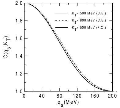
FIG. 1.: $\pi\pi$ Correlation Function x $q_{T}$ in Kinematical Zone I (side direction), showing the curves corresponding to the continuous emission with that corresponding to the sudden freezeout. This last case is not sensitive to $K_{T}$ in this kinematical zone but a slight dependence on $K_{T}$ can be seen for continuous emission.

Results corresponding to the ZONE I above are shown in Fig. 1. As expected, since we are neglecting the transverse expansion, the difference between the predictions of the two scenarios is small. Slightly broader correlation function for the CEM case, and the decreasing width with $K_{T}\,$, was also expected.

Case II (or Zone II) correponds to considering $\phi_{q}=0$, $|\vec{k}_{1}|>|\vec{k}_{2}|\,$, with both $\vec{k}_{i}$ along the $x$-axis, i.e., $\vec{k}_{i}\parallel\vec{K}_{T}\parallel\vec{q}_{T}$; in this case, we can write the individual momenta as $k_{i}^{\mu}=(\sqrt{m_{\pi}^{2}+[K_{T}\pm q_{T}/2]^{2}},K_{T}\pm q_{T}/2\,,0\,,0)$, where again the $\pm$ signs correspond to pion 1 and 2, respectively. The momentum difference $\vec{q}_{T}=\vec{q}_{O}$ in this situation corresponds to the so-called outwards compo-

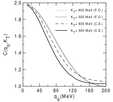
FIG. 2.: $\pi\pi$ Correlation Function x $q_{T}$ in Kinematical Zone II (out direction), showing the curves corresponding to the continuous emission with the ones corresponding to the sudden freezeout.

nent introduced in Ref[6, 7]. Results corresponding to the ZONE II above are shown in Fig. 2. This is the case, mentioned in the Introduction, where the duration of the emission process becomes essential[6, 7, 8, 9]. Since the emission time in the usual freezeout does not depend crucially on the particle momentum, the correlation function is almost independent of $K_{T}\,$. On the contrary, the emission time is strongly momentum dependent in

CEM, for large-momentum particles are emitted mainly at early times, whereas small-momentum particles may be emitted also at later stage of expansion when the fluid is cooler and the system larger. So, we see in Fig. 2 a significant $K_{T}\,$ dependence, being the correlation narrower for smaller $K_{T}\,$. Also, we can see that both the CEM curves are narrower than the corresponding freezeout curves, indicating that the emission time in CEM is longer in general. Looking more carefully at the curves, we can also perceive that the tail of $C(q_{T},K_{T})$ in CEM is much flatter than in sharp freezeout. Probably this flat tail is due to the small source depth in CEM at early times. It is clear that in Bjorken model without transverse expansion, which we used in the present work, the source depth is constant and $\sim R_{T}$ in sharp freezeout scenario.

Figure 3 represents the same situation as in Zone II but with a different freezeout temperature, $T_{fo}=140$ MeV, in order to show the sensitivity of the results for a lower $T_{fo}$ in the case of the usual freezeout. As seen, the $T_{fo}\,$ dependence has shown to be very weak, as expected.

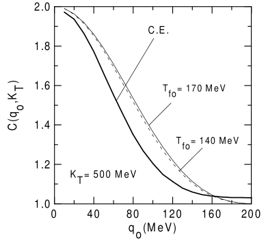
FIG. 3.: Study of the sensitivity to $T_{fo}$ in the abrupt freezeout model in the Kinematical Zone II (out direction). Together with previous results shown in Fig.2, the curve corresponding to a lower freezeout temperature, $T_{fo}=140MeV$, is also included.

B Averaged Correlations

Although the selective kinematical zones could teach us interesting points concerning the differences of the behavior of the correlation functions corresponding to both scenarios, as shown in Fig. 1-3, such conditions correspond to an idealization. For putting the calculations into more realistic grounds, averages over the angles, momenta, and the unobserved projections of the momentum differences $\vec{q}$ should be performed. Using the azimuthal symmetry of the problem we can still select $\vec{K}_{T}$ along the $x$-axis, such that $\vec{K}=(K_{T},0,K_{L})$. Then, averaging over different kinematical zones or windows would correspond to integrating over $\vec{K}$ and $\vec{q}$ (except over the plotting component of $\vec{q}$). In order to make the analysis roughly compatible with the range covered by NA35 S+A collisions[14], we considered the kinematical variables in the following intervals: $-0.5\leq y\leq 0.5$ (or, equivalently, $-180\leq K_{L}\leq 180$ MeV); $50\leq K_{T}\leq 600$ MeV; $0\leq(q_{L},q_{S},q_{out})\leq 30$ MeV (corresponding to the first experimental bin). As an illustration, we show below an example about how to compute the average:

$$\langle C(q_{L})\rangle=1+$$ (34)

$$\frac{\int_{-180}^{180}dK_{L}\int_{50}^{600}dK_{T}\int_{0}^{30}dq_{S}\int_{0}^{30}dq_{o}C(K,q)|G(K,q)|^{2}}{\int_{-180}^{180}dK_{L}\!\int_{50}^{600}dK_{T}\!\int_{0}^{30}dq_{S}\!\int_{0}^{30}dq_{o}C(K,q)G(k_{1},k_{1})G(k_{2},k_{2})}\,.$$ (35)

The results are presented in the following way. First, as done in the preceding subsection, in order to stress the differences of results predicted by the two scenarios under study, we start from the same initial temperature $T_{0}=200$ MeV for both the usual freezeout and CEM. The results are shown in Figs. 4-6, respectively as functions of $q_{L}\,$, $q_{O}$ and $q_{S}$. One sees in Fig. 4 that, as is well known, the $q_{L}$ dependence is very sensitive to the freeze-out temperature $T_{fo}$ and if the same initial temperature is attained in both scenarios, the correlation function cor-

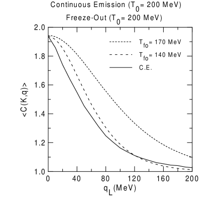
FIG. 4.: $\langle$ C $\rangle_{\pi\pi}$ x $q_{L}$ averaged over $q_{S}$ and $q_{o}$, showing the curve corresponding to the continuous emission hypothesis with the ones corresponding to the usual freezeout for $T_{fo}=170$ MeV and $T_{fo}=140$ MeV.

responding to the continuous emission picture is closer to the one referring to the thermal freezeout at lower $T_{fo}$. However, the shapes are not the same. The one related to CEM is more peaked at the small-$q_{L}$ values, becoming flatter in the tail region. This is in clear contrast to those corresponding to sharp freezeout scenario which are more similar to Gaussians. Physically, this behavior of CEM curve could be interpreted as exhibiting the history of the matter in expansion, because particles are emitted during the whole evolution in CEM. Namely, the tail of $\langle$C$\rangle$ depends essentially on early times, when the size of the fluid is small and its temperature high, whereas the peak reflects later times, when the fluid has fully expanded and cooled down.

We have already seen in the preceding subsection that, when plotted as function of $q_{O}\,$, the correlation function in CEM is significantly narrower than the one in the sharp freezeout and has a flatter tail. These features are again seen in Fig. 5, where $\langle C\rangle_{\pi\pi}$ with lower freeze-out temperature $T_{fo}\,$ is closer to the curve for CEM, as in Fig. 4. However, if the same initial temperature is attainded in both scenarios, very low $T_{fo}\,$ is necessary, in this case, in order to approximately reproduce the same correlation predicted by CEM. We can also notice that the depletion of the correlation function at small $q_{O}$ values is more dramatic in CEM. In any case, it is important to emphasize that our source is totally chaotic in both scenarios and, as is well known[6], $\langle C\rangle<2$ at $q_{L}=0$ is originated only from the averaging processes, since Coulomb final state interactions, as well as the effect of resonances decaying into $\pi$’s[8, 9] were not considered here.

We can again notice in Fig. 6 that, also as function of

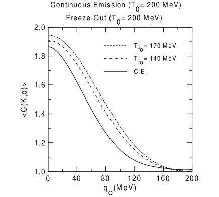
FIG. 5.: $\langle$ C $\rangle_{\pi\pi}$ x $q_{O}$ averaged over $q_{L}$ and $q_{S}$, showing the curve corresponding to the continuous emission hypothesis as compared to the ones corresponding to usual freezeout at $T_{fo}=170$ MeV and $T_{fo}=140$ MeV, but identical initial temperatures $T_{0}$.

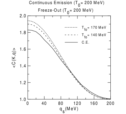
FIG. 6.: $\langle$ C $\rangle_{\pi\pi}$ x $q_{S}$ averaged over $q_{L}$ and $q_{O}$, showing the curve corresponding to the continuous emission hypothesis as compared to the ones corresponding to usual freezeout at $T_{fo}=170$ MeV and $T_{fo}=140$ MeV, but identical initial temperatures $T_{0}$.

$q_{S}\,$, the depletion of $\langle$ C $\rangle_{\pi\pi}$ is more pronounced in CEM as compared to the curves corresponding to the sharp freezeout case. As happened in the previous cases, for the same initial temperature, $\langle C\rangle_{\pi\pi}$ with lower $T_{fo}\,$ is closer to the curve for CEM, but the shape is somewhat different.

In the previous figures, we have shown and discussed the differences of CEM correlation function, confronted with the usual abrupt freezeout one, when the fluid started from the same initial conditions. Now, when analyzing the experimental data, the parameters are usually adjusted by fitting the data points as close as possible, and the conclusions are extracted from the adjusted parameters. In the present model calculations, the only parameter, besides the freezeout temperature $T_{fo}\,$, is the initial temperature $T_{0}$. For computing the results presented in Figs. 7-9, we have fixed the initial temperature for CEM as 200 MeV, and varied the initial temperature $T_{0}$ for the usual freezeout scenario, trying to get the same (or similar) result. To doing so, we have chosen the freezeout temperature as $T_{fo}=140$ MeV, as often done in hydrodynamic calculations and following the indications of the previous discussions.

As seen, especially in Fig. 7, the correlation functions predicted by the two different scenarios were so different in shape that it was not always possible to obtain similar curves. For example, in the case of $q_{L}$ dependence, Fig. 7, $\langle$C$\rangle$ for CEM is closer to the curve with higher $T_{0}$ at small $q_{L}$, but at high $q_{L}$, it turns to be closer to the one with the lowest value of $T_{0}$. As discussed above in connection with Fig. 4, the correlation curve in CEM could be interpreted as showing the history of the hot matter in expansion, i.e., the tail of $\langle$C$\rangle$ reflects essen-

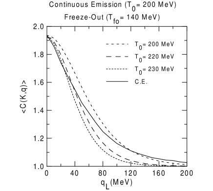
FIG. 7.: $\langle$ C $\rangle_{\pi\pi}$ x $q_{L}$ averaged over $q_{S}$ and $q_{O}$, showing the curve corresponding to the continuous emission hypothesis with the ones corresponding to the usual freeze-out at $T_{fo}=140$ MeV, but different initial temperatures $T_{0}$.

tially the early times, when the size of the fluid is small and its temperature high, and the peak the later times, when the fluid has fully expanded and cooled down. In the usual freezeout picture with a fixed $T_{fo}\,$, small $T_{0}$ is enough to produce a large tail, whereas a larger expansion, so higher $T_{0}\,$, is required to produce a narrower $\langle$C$\rangle$.

In Fig. 8, where the $q_{O}$ dependence of $\langle C\rangle_{\pi\pi}$ is shown, we can again observe a distortion introduced by CEM into the shape of the correlation function. We see that $\langle C\rangle$ for CEM is closer to the curve with $T_{0}=230$ MeV

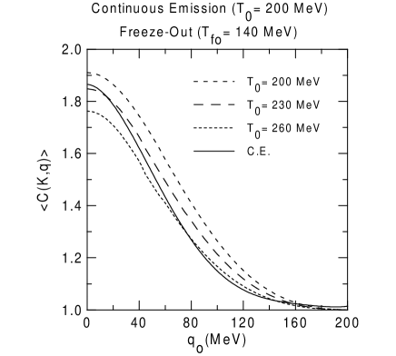
FIG. 8.: $\langle$ C $\rangle_{\pi\pi}$ x $q_{O}\,$, averaged over $q_{L}$ and $q_{S}$, showing the curve corresponding to CEM as compared to the ones corresponding to the sharp freezeout at $T_{fo}=140$ MeV, but different initial temperatures $T_{0}$.

at small $q_{O}$, but at high $q_{O}$, it turns to be closer to the one corresponding to $T_{0}=260$ MeV. However, differently from the previous case, Fig. 7, the shape of the freezeout correlation curves is only slightly dependent on $T_{0}$ and it becomes narrower as the temperature increases. What is clearly $T_{0}$ dependent here is the intercept at the origin, which reflects the large expansion dependence of $\langle C\rangle_{\pi\pi}$ x $q_{L}$ as shown in Figs. 4 and 7.

Finally, Fig. 9 shows that in this case it is possible to find an appropriate $T_{0}$ for sharp freezeout to reproduce the CEM curve. We see that $\langle$ C $\rangle$ for CEM is closer to the curve with $T_{0}=230$ MeV and the agreement is good for most of the $q_{S}$ region where the interferometric signal is present. This was expected because in the present study we neglected the transverse expansion, so the transverse size is the same in both the scenarios. The initial temperature $T_{0}$ in freezeout is higher than the one for CEM, because this is required to make the size of the fluid large enough and the correlation in the longitudinal direction sharp enough to decrease the intercept on averaging.

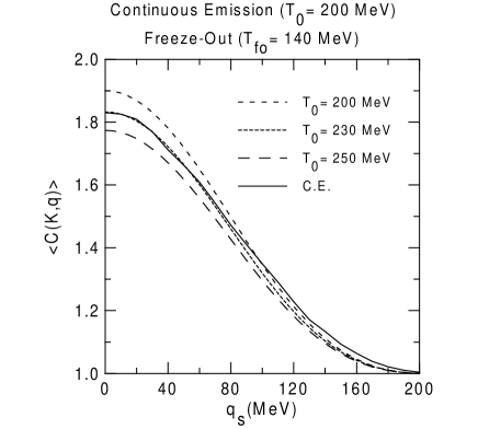
FIG. 9.: $\langle$ C $\rangle_{\pi\pi}$ x $q_{S}$ averaged over $q_{L}$ and $q_{O}$, showing the curve corresponding to CEM as compared to the ones corresponding to usual freezeout at $T_{fo}=140$ MeV, but with different initial temperature $T_{0}\,$.

From the above results, mainly from the correlation curves as function of $q_{L}\,$, we clearly see deviations from the pure Gaussian behavior in cases where the continuous emission ansatz was assumed. This could actually reflect a signature of a continuous process in the particle emission.

V Discussions and Concluding Remarks

As mentioned in the Introduction, treating the decoupling process in heavy-ion collisions as occurring on a sharply defined surface is an operationally simple but highly idealized description. If the consideration of a finite thickness of such a decoupling region does not bring any noticeable difference in the observable quantities, such an approximation would be unquestionable. However, previous studies[2, 3, 4, 5] have shown that several quantities, such as transverse spectra of produced particles and heavy-particle production ratios are sensitive to more involved description of the process, called continuous emission model[2].

In this paper, we concentrated on the two-pion interferometry, which has extensively been used as a powerful tool for extracting the space-time geometry, as well as probing the underlying dynamics of the hadronic matter formed in heavy-ion collisions, and studied the differences introduced by CEM in confront with the usual sudden freezeout. As shown in Sec. IV, also the HBT effect suffers a large deformation when the usual freezeout is replaced by CEM. This means that conclusions achieved on the properties of the matter formed in high-energy collisions may differ substantially if we adopt one or the other scenario studied here.

For the sake of conceptual clarity and, evidently, also to simplify the computation, we have adopted in this work a simplified one-dimensional Bjorken model for massless pion fluid (the pion mass has been included only to computing observable quantities), without phase transition. Nevertheless, one general result emerges, which seems to be evident especially by looking at Figs. 7-9. Namely, if we describe the same data by using CEM or sharp freeze-out (with $T_{fo}=140$ MeV), the initial temperature $T_{0}\,$ required in CEM is lower than in the usual freeze-out. If $T_{fo}$ is higher, the difference in $T_{0}$ becomes even larger, which is clear from Figs. 4-6. This result means that if CEM is the correct description of the decoupling process, then it is harder to reach the quark-gluon plasma phase than it appears in the usually adopted sharp freezeout scenario.

Since we have worked with a simplified model, we did not attempt to make any comparison with data. For doing this, evidently we have to do some (or all) of the following improvements. More realistic equation of state (probably including phase transition) should be used; finite longitudinal extension of the fluid should be considered; transverse expansion should be included; resonance formation should be taken into account. All these modifications require some hydrodynamic numerical code with CEM incorporated. We are now working in this direction.

Acknowledgement

This work was partially supported by FAPESP (contract nos. 1998/02249-4 and 1998/14990-0) and by CNPq (contract no. 300054/92-0). We express our gratitude to T. Kodama and T. Csörgő for stimulating discussion on the results.

REFERENCES

- [1] F. Cooper and G. Frye, Phys. Rev. D10 (1974) 186.
- [2] F. Grassi, Y. Hama and T. Kodama, Phys. Lett B355 (1995) 9; Z. Phys. C73 (1996) 153.
- [3] F. Grassi, Y. Hama, T. Kodama and O. Socolowski Jr., Heavy Ion Phys. 5 (1997) 417.
- [4] F. Grassi and O. Socolowski Jr., Phys. Rev. Lett. 80 (1998) 1170; F. Grassi and O. Socolowski Jr., J. Phys. G25 (1999) 331.
- [5] F. Grassi and O. Socolowski Jr., J. Phys. G25 (1999) 339.
- [6] Yogiro Hama and Sandra S. Padula, Phys. Rev. D37 (1988) 3237.
- [7] S. Pratt, Phys. Rev. D33 (1986) 1314 ; G. Bertsch, M. Gong and M. Tohyama, Phys. Rev. C37 (1988) 1896; T. Csörgő and J. Zimanyi, Nucl. Phys. A527 (1991) 621c; S. Chapman, J.R. Nix and U. Heinz, Phys. Rev. C52 (1995) 2694; T. Csörgő and B. Lörstad, Nucl. Phys. A590 (1995) 465; U. Heinz, B. Tomasik, U.A. Wiedermann and Y.F. Wu, Phys. Lett. 382B (1996) 181.
- [8] Miklos Gyulassy and Sandra S. Padula, Phys. Lett. 217B (1989) 181.
- [9] Sandra S. Padula, M. Gyulassy and S. Gavin, Nucl. Phys. B329 (1990) 357 ; Sandra S. Padula and M. Gyulassy, Nucl. Phys. B339 (1990) 378.
- [10] J.D. Bjorken, Phys. Rev. D27 (1983) 140.
- [11] W.A. Zajc, Hadronic Multiparticle Production, World Scientific Press, P. Carruthers, ed. (1988); D.H. Boal, C.K. Gelbke and B.K. Jennings, Rev. Mod. Phys. 62 (1990) 553; C-Y. Wong, Introduction to High-Energy Heavy-Ion Collisions, World Scientific (1994); R.M. Weiner, Bose-Einstein Correlations in Particle and Nuclear Physics, J. Wiley & Sons (1997); U. Heinz and B. V. Jacak, Ann. Rev. Nucl. Part. Sci. 49 (1999) 529; T. Csörgő, hep-ph/0001233.
- [12] M. Gyulassy, S.K. Kaufmann, and L.W. Wilson, Phys. Rev. C20 (1979) 2267; K. Kolehmainen and M. Gyulassy, Phys. Lett. B180 (1986) 203.
- [13] Sandra S. Padula and Cristiane G. Roldão, Phys. Rev. D58 (1998) 2907.
- [14] T. Alber et al., Z. Phys. C66 (1995) 77.