Scaling and Duality in Semi-exclusive Processes

Abstract

We discuss extending scaling and duality studies to semi-exclusive processes. We show that semi-exclusive hard pion photoproduction should exhibit scaling behavior in kinematic regions where the photon and pion both interact directly with the same quark. We show that such kinematic regions exist. We also show that the constancy with changing momentum transfer of the resonance peak/scaling curve ratio, familiar for many resonances in deep inelastic scattering, is also expected in the semi-exclusive case.

WM-00-102; hep-ph/0002271

I Introduction

Scaling is a well established phenomenon in deep inelastic scattering (DIS). The cross section with specific kinematic factors removed gives structure functions that depend on only the scaling variable $x_{B}$, up to calculable logarithmic corrections. In addition, an inclusive-exclusive connection—“Bloom-Gilman scaling” [1]—is observed in these totally inclusive (at least on the hadronic side) reactions. Duality in this situation means that resonance bumps observed in the structure functions at low momentum transfers $Q^{2}$ average out to the smooth structure function measured at higher momentum transfers but the same $x_{B}$. Usually, but not always, duality is realized in such a way that as the resonance peak moves in $x_{B}$ with changing $Q^{2}$, the ratio of the peak height to the height of the scaling curve evolved from higher $Q^{2}$ is constant.

Both scaling and scaling violation have played a crucial role in understanding the constituents of elementary particles and in establishing QCD as as the accepted theory of the strong interactions. Duality is in detail less well understood [2, 3]. It seems, however, to show that the fundamental single quark QCD process is still decisive in setting the scale of the reaction in the resonance region, and that the crucial role of the final state interactions in forming the resonance becomes moot when averaged over, say, the resonance width. This last observation, if reliably understood, could allow one to use duality to study the structure functions in the interesting and still experimentally uncertain $x_{B}\rightarrow 1$ region. For a fixed available energy, $x_{B}\rightarrow 1$ means getting into the resonance region and if one were sure of the connection of the resonance region average to the scaling curve, one could determine the scaling curve significantly closer to the kinematic upper endpoint.

Departing from DIS, we want to continue test our ability to understand and apply QCD to describe hadronic processes. A set of processes that can be a new testing ground for both scaling and duality phenomena are semi-exclusive reactions typified by

$$\gamma+p\rightarrow\pi+X,$$ (1)

where the photon may be real or virtual. These processes are the topic of this paper. We shall study suitable kinematic variables for the general case and, when we get more detailed, give special attention to photoproduction with large photon to pion momentum transfer, $t$.

A first requirement is to find a scaling region. This problem has been studied in the high $Q^{2}$–low $(t/Q^{2})$ limit, focusing on the totally exclusive reaction but with extension to the semi-exclusive case [4]. These authors found that scaling functions would exist, provided the photon and pion currents directly and successively interacted with the same quark while the rest acted as spectators.

We here, concentrating on photoproduction at high $|t|$, show that perturbative QCD (pQCD) predicts there is indeed a scaling region. We shall below show the kinematic factors that connect the cross section to the expected scaling function. We shall also see that the scaling region does require kinematics where photopion production is dominated by direct interactions of both the photon and the pion [5, 6, 7], such as seen in Fig. 1. In particular, one must avoid regions where the pion comes from soft processes or comes as part of a jet from a fragmenting parton. In earlier work we were able to show that regions of direct pion production exist, and therefore there are regions where we can find a scaling function.

When scaling is established at high $|t|$, one can study duality. One can ask whether the scaling curve from high $Q^{2}$ or $t$ a decent average over the resonance bumps seen at the same $x$ but lower $Q^{2}$ or $t$? Duality in this sense appears to be true for all the resonances seen in DIS. Further, one can ask if the bump to continuum ratio is constant as $Q^{2}$ or $t$ changes? This constancy is seen in DIS for most resonances, but not for the $\Delta$(1232). While studying the kinematics and working in photoproduction context, we will see that it is possible in a single experiment with good kinematic coverage to probe a given $x$ region over a wide range of $m_{X}$ from the resonance region to well into the continuum region.

The paper proceeds as follows. Section II will discuss the kinematics and scaling variable for the semiexclusive process. Section III will show how a scaling function emerges for semi-exclusive hard pion photoproduction, and also show the existence of a region where direct pion production dominates, specifically for a situation of 30 GeV incoming photons. Section IV will show that pQCD expectations for the resonance peak/scaling curve ratio at changing $|t|$ are similar to what one sees in DIS. Section V will offer some conclusions.

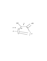
FIG. 1.: Direct (also isolated or short-distance) pion production, with some kinematics indicated.

II kinematic variables

For the process $\gamma+p\rightarrow\pi+X$, define the Mandelstam variables by

$$s=(p+q)^{2},\quad t=(q-k)^{2},\quad u=(p-k)^{2}\ .$$ (2)

Define $x$ in general by,

$$x={-t\over s+u-2m_{N}^{2}-q^{2}-m_{\pi}^{2}},$$ (3)

and note that all quantities defining $x$ are experimentally measurable [5, 6, 7]. One can show $0\leq x\ \leq 1$, and $x=1$ corresponds to the case that $X$ is a nucleon. Also generally, the hadronic mass recoiling against the pion is given by

$$m_{X}^{2}=m_{N}^{2}-t\left({1\over x}-1\right).$$ (4)

Specializing to the case where direct pion production, Fig. 1, is the underlying process, in the limit of high $t$ or $s$ and high recoil mass $m_{X}$, one can show that this $x$ is the fraction of the target’s momentum carried by the struck quark. The proof involves defining Mandelstam variables for the subprocess $\gamma+q\rightarrow\pi+q^{\prime}$. We anticipate the result by letting the momentum of the struck quark be called $xp$, and get

$$\hat{s} = (xp+q)^{2}=x(s-q^{2})+q^{2}\ ,$$ (5)

$$\hat{t} = (q-k)^{2}=t\ ,$$ (6)

$$\hat{u} = (xp-k)^{2}=xu\ ,$$ (7)

where we have neglected masses but not $q^{2}$. For the direct pion production subprocess,

$$\hat{s}+\hat{t}+\hat{u}=q^{2}\ ,$$ (8)

and substituting Eqn. (5) leads to the identification of $x$ the momentum fraction to $x$ the experimental observable, when individual particle masses can be neglected.

Thus $x$ is a precise analog of the observable $x_{B}=Q^{2}/2m_{N}\nu$ in deep inelastic scattering. Our formulas should and do connect to the well known ones for deep inelastic kinematics in the limit $k\rightarrow 0$. In this limit, $u\rightarrow m_{N}^{2}$ and $t\rightarrow q^{2}\equiv-Q^{2}$ and

$$m_{X}^{2} = m_{N}^{2}+Q^{2}\left({1\over x}-1\right)\ ,$$ (9)

$$x = {-t\over s-m_{N}^{2}-q^{2}}={Q^{2}\over 2p\cdot q}\ ,$$ (10)

without approximation.

Still regarding deep inelastic scattering, Bloom and Gilman [1] found that near threshold scaling worked better if one used a revised variable defined as $1/x^{\prime}_{B}=1/x_{B}+m_{N}^{2}/Q^{2}$. By analogy to Bloom and Gilman’s proposal we could define a modified scaling variable with $-t$ replacing $Q^{2}$:

$${1\over x^{\prime}}={1\over x}+{m_{N}^{2}\over-t},$$ (11)

whence

$$m_{X}^{2}=-t{1-x^{\prime}\over x^{\prime}}.$$ (12)

One should keep this possibility in mind here also.

Another situation, related to the one we are pursuing, is semi-exclusive deep inelastic scattering with parallel kinematics. This means high $Q^{2}$ and an observed meson with three-momentum parallel to the incoming photon, in the lab. In this case, there is a variable $z$ defined by

$$z\equiv{p\cdot k\over p\cdot q}\ .$$ (13)

and obtain

$$m_{X}^{2} = m_{N}^{2}+Q^{2}(1-z)\left({1\over x}-1\right)\ ,$$ (14)

$$x = {Q^{2}\over 2p\cdot q}\ ,$$ (15)

with the neglect of terms of ${\cal O}(m_{N}^{2}x^{2}/Q^{2})$.

III scaling and kinematic regions

Now we shall focus on hard pion photoproduction, where $q^{2}=0$, $k_{T}$ is large, and $|t|$ is large.

We will be mainly interested in direct pion production with $m_{X}$ large, and in the transition to the exclusive reactions $\gamma+N\rightarrow\pi X$. Other processes do contribute. In particular there are soft processes, and processes where the pion is produced as part of the fragmentation of a quark or gluon into a jet. These processes can be evaded if one can go to sufficient transverse momentum. We will comment on them briefly before proceeding.

Soft processes are frequently approximated using vector meson dominance of the photon interaction, illustrated in Fig. 2. They are important at low transverse momenta, although the boundary between “low” and “high” is higher than one might expect, namely around 2 GeV. We have considered these processes in a fashion suitable for the present context in [8]; one can also find a representation of them in PYTHIA [9].

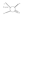
FIG. 2.: Soft processes, approximated by vector meson dominance.

Moderate transverse momenta hard pions can be produced by a fragmentation of a parton. The process is perturbatively calculable and could be a way to learn about polarized of unpolarized gluon distributions of the target [6, 10]; one example is illustrated in Fig. 3.

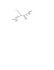
FIG. 3.: A fragmentation process, where the pion is labeled as having momentum $k$.

Neither the fragmentation nor the soft process is useful for the present duality study. The reason is that the experimental $x$ variable for them does not have a unique connection to the quark momentum fraction, and we will not be able to prove a scaling relation for them.

Direct pion production, however, does have the nice connection between an experimentally observable $x$ and the struck quark momentum fraction, and it is calculable in pQCD. It is a higher twist process. Factors of the decay constant enter the amplitude, representing the quark-antiquark wave function of the pion at the origin, and must be dimensionally compensated by an extra power of $s$ in the cross section. Nonetheless, it can dominate over fragmentation at high $k_{T}$ because it always gives all the transverse momentum in the pion direction to the one pion. For the direct process, we can operationally define a scaling function $F(x,t)$ by

$$E_{\pi}{d\sigma\over d^{3}k} = {(s-m_{N}^{2})x^{2}\over-\pi t}{d\sigma\over dx\,dt}$$ (16)

$$= {(s-m_{N}^{2})x^{2}\over-\pi t}\ {d\hat{\sigma}\over dt}(\gamma q\rightarrow\pi q^{\prime})\ F(x,t)\ .$$ (17)

I.e., the scaling function is related to the cross section by some kinematic factors, which are partly explicit above and partly given in terms of the cross section for the subprocess

$${d\hat{\sigma}(\gamma q\rightarrow Mq^{\prime})\over dt} = {128g_{F}^{2}\pi^{2}\alpha\alpha_{s}^{2}\over 27(-t)\hat{s}^{2}}I_{M}^{2}\left({e_{q}\over\hat{s}}+{e_{q^{\prime}}\over\hat{u}}\right)^{2}$$ (18)

$$\times \left[\hat{s}^{2}+\hat{u}^{2}+\lambda h\left(\hat{s}^{2}-\hat{u}^{2}\right)\right],$$ (19)

where we should substitute quark charges relevant for pion being produced, for example $e_{q}=e_{u}$ and $e_{q}^{\prime}=e_{d}$ for the $\pi^{+}$. The flavor factor $g_{F}$ is unity for the $\pi^{\pm}$ and $1/\sqrt{2}$ for the $\pi^{0}$. $I_{M}$ is for the present purpose a constant factor, but if the perturbative calculation is valid, it will be given in terms of the distribution amplitude of the meson as $\int d\xi_{1}\,\phi_{M}(\xi,\mu^{2})/\xi_{1}$. For the asymptotic distribution amplitude, $I_{\pi}=\sqrt{3}f_{\pi}/2$ with $f_{\pi}\approx 93$ MeV.

We have included polarization dependence for future use: $\lambda$ is the helicity of the photon and $h$ is twice the helicity of the target quark. Of course, duality can be tested with polarization as well as without.

The reason to believe that the above expression, Eqn. (16), produces a scaling formula is that the perturbative formula valid for short distance pion production (the process of Fig. 1) is,

$$E_{\pi}{d\sigma\over d^{3}k} = {(s-m_{N}^{2})x^{2}\over-\pi t}$$ (20)

$$\times \sum_{q}{d\hat{\sigma}\over dt}(\gamma q\rightarrow\pi q^{\prime})\,G_{q/T}(x,\mu^{2})$$ (21)

Thus where perturbation theory works, there is a scaling function $F(x,t)$ is mainly dependent on $x$. We can relate it to the quark distributions (with weak dependence on the scale $\mu^{2}$, which we may set to $t$), as in DIS. We expect the formulas will be mainly applied in the high $x$ region, where valence quarks dominate. Hence the comment on the choice of the quark charges just above.

Let us comment on the fact that the presence of a hard gluon exchange (see Fig. 1) indicates that one needs sufficiently high energies to apply the pQCD formalism. However, since only one pion distribution amplitude is involved for the direct process, if the photon attaches to the produced $q\bar{q}$ pair of Fig. 1 (the worse case), the average virtuality of the gluon in question corresponds to the one determining the pion electromagnetic form factor at $Q^{2}\approx 20(35)$ GeV² scale, for the asymptotic (Chernyak-Zhitnitsky) pion distribution amplitude assuming a CEBAF energy of 12 GeV, pion emission angle of 22^∘, and $m_{X}=2$ GeV (see Ref. [6] for details). Therefore one may hope to observe a single-gluon exchange, which is a higher twist effect, in inclusive photoproduction of pions even at CEBAF energies generally considered not high enough to reach the perturbative QCD domain. Indications of direct pion production off a quark were obtained in $\pi N$ scattering (see Ref. [11] for references and discussion).

We may now ask if this scaling function dual, in a Bloom-Gilman like sense, to the bumpier curve one will get in the resonance region? The resonance region, of course, is what we have at the very highest transverse momentum, where there is very little energy left over to put into recoil mass.

Formally, the duality relation then may be written as an integral of the differential cross section $d\sigma/dx\,dt(\gamma N\rightarrow\pi X)$ and in the region of the direct process dominance reads

$$\int_{(1-{m_{X}^{2}-m_{N}^{2}\over t})^{-1}}^{1} dx \,\sum_{q}G_{q/N}(x){d\sigma\over dt}(\gamma q\rightarrow\pi q^{\prime})$$ (22)

$$\propto \sum_{R} {d\sigma\over dt}(\gamma+N\rightarrow\pi+R)\ .$$ (23)

Summation in the right hand side of Eqn. (22) is done over all resonances $R$ with masses $m_{R}\leq m_{X}$, with the nucleon final state included. If the parton distribution function of the nucleon is $G_{q/N}\sim(1-x)^{3}$ at $x\rightarrow 1$ and the subprocess $\gamma q\rightarrow\pi q^{\prime}$ cross section is determined by the one-gluon exchange mechanism of Fig. 1, then as will be shown in the next section duality as in Eqn. (22) requires that the resonance excitation cross section ${d\sigma/dt}(\gamma+N\rightarrow\pi+R)\propto 1/s^{7}$ at fixed $t/s$—the result known from the constituent counting rules [12]. The duality relation above could also be written using the modified scaling variable $x^{\prime}$ from Eqn. (11).

One should ask if the proper regions exist. There needs to be a region where direct pion production dominates, where one can measure the scaling curve and see how it tails off into the resonance region. Such a region does exist. ¿From earlier studies [6, 8] we have the machinery to calculate the direct pion and fragmentation process, and estimate the VMD processes, and have shown that the direct process, even though it is higher twist, does take over at some point if we have enough initial photon energy.

A useful presentation of our calculated results is shown in Fig. 4. The figure attempts to show that we can follow a given $x$ region from the resonance region until well into the scaling region, and do so in a single experiment. The axes of Fig. 4 give the outgoing pion transverse and longitudinal momenta, in the target rest frame. Some labeled straight lines give the pion angle relative to the incoming beam. The three solid elliptical curves each correspond to a fixed value of recoil mass $m_{X}$. The outermost curve has $m_{X}=m_{N}$ and thus corresponds to the quasielastic process $\gamma N\rightarrow\pi N$, and also marks the kinematic limit of pion momenta. The next curve has $m_{X}=2$ GeV, and the innermost solid curve has $m_{X}=3.5$ GeV. Thus the region between the two outermost curves is the resonance region, and the region within the middle solid curve is the continuum region. The segment above the grey band is the region where direct pion production dominates. For us, this is the “good region.” (As a side note, the grey band is straighter than we might have guessed, especially since it is made up of two parts. The central part comes from the fragmentation process growing larger. Both ends come from VDM, as modeled in an earlier note, which we think was conservative in estimating the size of the VDM contributions.) Finally comes the important dotted elliptical curve, which has a constant $x$, specifically $x=0.7$ in this case. We see that we can thinkably measure the putative scaling function in the resonance region at small pion angles, and then by moving to larger angle, follow its behavior at the same $x$ but larger $m_{X}$ (and larger $|t|$) well out of the resonance region, before running into a region where fragmentation or soft processes dominate.

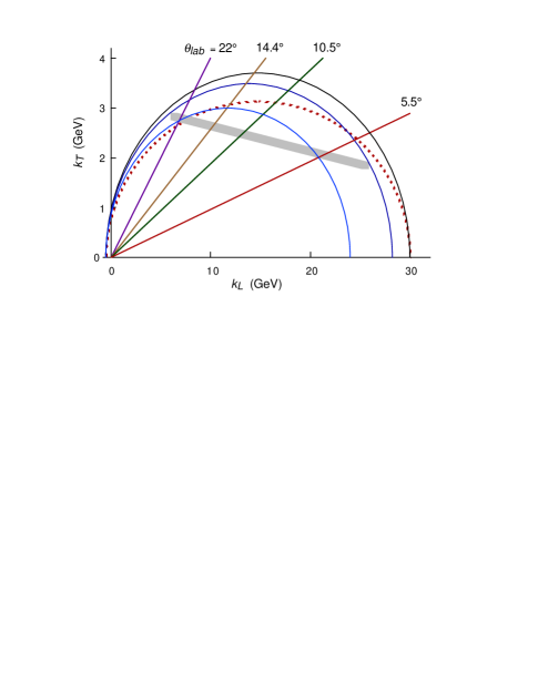
FIG. 4.: Kinematic regions relevant to studying duality in $\gamma N\rightarrow\pi X$ for 30 GeV incoming photons. The upper solid elliptical line is the overall kinematic limit, and corresponds to $\gamma N\rightarrow\pi N$. The other two solid elliptical lines have $m_{X}$ of 2 and 3.5 GeV, respectively. Between the two upper solid elliptical lines lies the resonance region. Above the grey line soft processes and fragmentation processes are small, and direct pion production dominates. Hence the region between the grey line and the middle elliptical line is the region that can be smoothly compared to the resonance region. The dotted elliptical curve is for $x$ fixed at 0.7.

(As another aside, lines of constant $|t|\neq 0$ on this plot would be parabolas opening to the right, and passing through the small line segment between the origin and the lower (negative) limit of $k_{L}$; $|t|=0$ occurs along the positive $k_{L}$ axis.)

IV resonance bumps vs. the scaling curve

There is always a resonance region. In plots of $F(x,t)$ vs. $x$, the bumpy resonance region slides to the right with increasing $|t|$. In the corresponding DIS case the bumps slide neatly down the curve, with the resonance/smooth curve ratio observed to stay the same, for most resonances. Within pQCD, this is expected theoretically [3] as a consequence of the known behaviors of the scaling curve as $x\rightarrow 1$ and the predicted falloff of the resonance transition form factors at high $Q^{2}$. We can show that the resonance/continuum constancy is consistent with pQCD in the semi-exclusive case also.

We need to find the behavior of

$$F_{res}(x,t)={d\sigma\over dx\,dt}(\gamma N\rightarrow\pi R)/{d\sigma\over dt}(\gamma q\rightarrow\pi q^{\prime})$$ (24)

at (say) the resonance peak for large $|t|$ (and $x\rightarrow 1$). The denominator in this limit is

$${d\sigma\over dt}=g(t/s)|t|^{-3}\propto(1-x)^{3}$$ (25)

where $g(t/s)$ is a known function (see Eqn. (18)) which does not go to zero for $t/s$ finite, and we have used $1/t\propto(1-x)$ in the stated limit.

The numerator for a finite width resonance can be approximated by (for $x\rightarrow 1$),

$$\left(d\sigma\over dx\,dt\right)_{res} \approx {|t|\over 2m_{X}}\left(d\sigma\over dm_{X}\,dt\right)_{res}$$ (26)

$$\approx {|t|\over 2m_{R}}\left(d\sigma\over dt\right)_{res}{\Gamma/2\pi\over(m_{X}-m_{R})^{2}+\Gamma^{2}/4}$$ (27)

where $\Gamma$ is the width of the resonance and we have used a simple lorentzian form to give the resonance shape. The pQCD scaling rules [12] tell us that

$$\left(d\sigma\over dt\right)_{res}=f(t/s)|t|^{-7}$$ (28)

where $f(t/s)$ is not known but in general it should not go to zero for finite $t/s$. Thus,

$$\left(d\sigma\over dx\,dt\right)_{res\ peak}\approx{1\over\pi m_{R}\Gamma}f(t/s)|t|^{-6}\propto(1-x)^{6}$$ (29)

Thus,

$$F_{res\ peak}(x,t)\propto(1-x)^{3}\ .$$ (30)

This is how the height of a resonance peak fall with $x$ as $x\rightarrow 1$. It is also precisely the pQCD expectation for the scaling curve. Hence the resonance/continuum ratio is in general constant, at least at high $|t|$, as it is for DIS.

In DIS, the Delta(1232) is an exception, as it falls markedly with $Q^{2}$ [13, 14]; $Q^{2}$ in lepton scattering is the analog of $-t$ in hard meson photoproduction. It will be interesting to see if the Delta(1232) disappears with increasing $|t|$ and if the, say, S₁₁(1535) stays up at high $|t|$. Recall that in pQCD, the disappearing Delta in electron scattering is explained as an accident having to do with the specifics of the Delta and nucleon wave functions [15]. We should not expect this to be necessarily replicated in pion photoproduction since the integrals over the distribution amplitudes will involve different weightings.

V Conclusions and Discussion

Semi-exclusive processes give an opportunity to extend the studies of scaling and duality, which in deep inelastic scattering have been fruitful in verifying our understanding of QCD and in pushing our effort to deepen that understanding.

It appears that scaling in the sense that the cross section is directly related to a scaling function that depends, up to logarithmic corrections, on just one variable. The scaling variable for semi-exclusive processes, given in the text, is related to the momentum fraction of the struck quark, just like the scaling variable in deep inelastic scattering. However, scaling, at least as we have been able to present it in this paper, works in semi-exclusive process only when the pion is produced directly off the same quark that absorbs the incoming photon. We have been able to show, theoretically, that such a scaling region does exist.

One should bear in mind that there are soft kinematic regions where one does not know where the pion comes from, and fragmentation regions where the pion is produced at some remove from the fundamental process that initiates the reaction. We do not know of a scaling function for these regions, and it is not trivial that one can avoid them, but one can. One should also bear in mind that a certain amount of initial energy is needed to be able to produce a scaling region. For incoming photon lab energy 16 GeV or below and our present estimates of the vector meson dominance contributions, it does not appear that there is a region where VMD is not the biggest process for photoproduction, at least if one does not make any additional cuts. However, a there are possibilities for reducing the necessary incoming energy. One follows from noting that a directly produced pion is also a pion produced in kinematic isolation, not as part of a jet, and one can consider an “isolation cut,” a requirement that there be no other particles collinear with the pion. Another possibility is to have the photon off shell, since then the vector meson propagator is significantly reduced, reducing the VMD contributions without there being an equal reduction for other contributions. We are hopeful that using electroproduction and isolation cuts can make the incoming energy requirement low enough to fit an upgraded CEBAF range, but are deferring detailed elaboration.

The existence of a scaling region also allows one to consider the inclusive-exclusive connection with the resonance region. Will the resonance bumps average out to the smooth scaling curve measured at higher $-t$ and evolved to lower $-t$ [16]? Will the resonance peak to scaling curve ratio be independent of $t$? In deep inelastic physics, it does appear that the final state interactions which produce the resonance are irrelevant to the overall rate of resonance region production, if one does a suitable average. And we have shown that for the semi-exclusive case, as in the deep inelastic case, the resonance to continuum ratio should be constant, barring special circumstances. A special circumstance in the deep inelastic case occurs for the $\Delta(1232)$, which disappears into the scaling curve with increasing $Q^{2}$. One would like to know if similar phenomena occur in other situations.

Testing scaling and duality in inclusive photoproduction of mesons requires coverage of the large-$x$ region, where the cross sections are rapidly falling as $x$ approaches it upper limit. Therefore such a uniquely designed high-luminosity machine as CEBAF, with a bit more energy, could do an excellent job in these duality studies.

We thank Nathan Isgur, Wally Melnitchouk, Chris Armstrong, Rolf Ent, and Cynthia Keppel for useful discussions about duality and give the latter three a second thanks for showing us their experimental duality results from CEBAF. AA thanks the US Department of Energy for support under contract DE-AC05-84ER40150; CEC and CW thank the NSF for support under grant PHY-9900657.

REFERENCES

- [1] E. D. Bloom and F. J. Gilman, Phys. Rev. Lett. 25 (1970) 1140; Phys. Rev. D 4 (1971) 2901.
- [2] A. DeRújula, H. Georgi, and H. D. Politzer, Ann. Phys. (N. Y.) 103, 315 (1977).
- [3] C. E. Carlson and N. C. Mukhopadhyay, Phys. Rev. D 41, 2343 (1990).
- [4] N. Dombey and R. T. Shann, Phys. Lett. B 42, 486 (1972); G. B. West, Phys. Lett. B 46, 486 (1973); A. Calogeracos, N. Dombey, and G. B. West, hep-ph/9406269.
- [5] C. E. Carlson and A. B. Wakely, Phys. Rev D 48, 2000 (1993).
- [6] A. Afanasev, C. E. Carlson, and C. Wahlquist, Phys. Lett. B 398, 393 (1997) and Phys. Rev.D 58, 054007 (1998).
- [7] S. J. Brodsky, M. Diehl, P. Hoyer, S. Peigne, Phys. Lett. B 449, 306 (1999).
- [8] A. Afanasev, C. E. Carlson, and C. Wahlquist, Phys. Rev.D 61, 054007 (2000).
- [9] T. Sjöstrand, Comput. Phys. Commun. 82, 74 (1994).
- [10] D. De Florian and W. Vogelsang, Phys. Rev. D 57, 4376 (1998); B. A. Kniehl, Talk at Ringberg Workshop, hep-ph/9709261; M. Stratmann and W. Vogelsang, Talk at Ringberg Workshop, hep-ph/9708243; J. J. Peralta, A. P. Contogouris, B. Kamal and F. Lebessis, Phys. Rev. D 49, 3148 (1994).
- [11] J. F. Owens, Rev. Mod. Phys. 59, 465 (1987).
- [12] S. J. Brodsky and G. Farrar, Phys. Rev. Lett. 31, 1153 (1973), Phys. Rev. D 11, 1309 (1975); V. A. Matveev, R. M. Muradyan, and A. N. Tavkhelidze, Lett. Nuovo Cimento 7, 719 (1973).
- [13] P. Stoler, Phys. Rev. Lett. 66 1003 (1991); Phys. Rev. D 44 73 (1991); Phys. Rep. 226, 103 (1993); G. Sterman and P. Stoler, Ann. Rev. Nucl. and Part. Sci. (in press).
- [14] C.E. Carlson and N.C.Mukhopadhyay, Phys. Rev. D 47 (1993) R1737.
- [15] C.E. Carlson and J.L. Poor, Phys. Rev. D 38, 2758 (1988); G.R.Farrar, H. Zhang, A.A. Oglublin, and I.R. Zhitnitsky, Nucl. Phys. B 311, 585 (1989); J. Bonekamp, Bonn report(1989).
- [16] This paper will not discuss whether the structure functions evolve or have reduced evolution at high and low . The question has been raised in, e.g., S. J. Brodsky, T. Huang, and G. P. Lepage, Proceedings of the Banff Summer Institute on Particles and Fields, Banff, Canada, Aug. 16-27, 1981, edited by A. Z. Capri and A. N. Kamal (Plenum Press, 1983), pp. 143-199 (see especially pp. 177-178).