Abstract

For an intermediate mass Higgs boson with SM-like couplings the LHC allows observation of a variety of decay channels in production by gluon fusion and weak boson fusion. Cross section ratios provide measurements of various ratios of Higgs couplings, with accuracies of order 15% for 100 fb^-1 of data in each of the two LHC experiments. For Higgs masses above 120 GeV, minimal assumptions on the Higgs sector allow for an indirect measurement of the total Higgs boson width with an accuracy of 10 to 20%, and of the $H\to WW$ partial width with an accuracy of about 10%.

Abstract

We discuss the production of neutral Higgs bosons at the hadron colliders Tevatron and LHC, in the context of the Standard Model and its minimal supersymmetric extension. The main focus will be on the next–to–leading order QCD radiative corrections to the main Higgs production mechanisms and on Higgs production in processes of higher order in the strong coupling constant.

Abstract

We analyze the signatures of the charged Higgs particles of the Minimal Supersymmetric extension of the Standard Model at the LHC. We will mainly focus on the large $M_{H^{\pm}}$ range where the charged Higgs boson is produced through the gluon–bottom or gluon–gluon mechanisms. The resulting $H^{\pm}$ signal is analyzed in its dominant $H^{+}\to tb$ as well as subdominant decay channels. Simulations for the detection of the charged Higgs boson signals in the decay channels $H^{\pm}\to\tau^{\pm}\nu$ and $H^{\pm}\to cs,W^{\pm}h$ or $tb$ are performed in the framework of the CMS and ATLAS detectors, respectively.

Abstract

We analyze the effects of light top squarks with large mixing on the search of the lightest Higgs boson of the Minimal Supersymmetric extension of the Standard Model at the LHC. We discuss both the stop loop effects in the main production and decay processes, and the associated production of top squarks with the lightest Higgs boson.

Abstract

The reconstruction of the Higgs potential in the Minimal Supersymmetric Standard Model (MSSM) requires the measurement of the trilinear Higgs self-couplings. The ‘double Higgs production’ subgroup has been investigating the possibility of detecting signatures of processes carrying a dependence on these vertices at the Large Hadron Collider (LHC) and future Linear Colliders (LCs). As reference reactions, we have chosen $gg\to hh$ and $e^{+}e^{-}\to hhZ$, respectively, where $h$ is the lightest of the MSSM Higgs bosons. In both cases, the $Hhh$ interaction is involved. For $m_{H}\lower 3.01385pt\hbox{$\;\stackrel{{\scriptstyle\textstyle>}}{{\sim}}\;$}2m_{h}$, the two reactions are resonant in the $H\to hh$ mode, providing cross sections which are detectable at both accelerators and strongly sensitive to the strength of the trilinear coupling involved. We explore this mass regime of the MSSM in the $h\to b\bar{b}$ decay channel, also accounting for irreducible background effects.

Abstract

The search strategies for Higgs bosons at LEP, Tevatron, LHC and future $e^{+}e^{-}$ linear colliders (LC) and muon colliders exploit various Higgs boson production and decay channels. The strategies depend not only on the experimental setup [e.g. hadron versus lepton colliders] but also on the theoretical scenarii, for instance the Standard Model (SM) or some of its extensions such as the Minimal Supersymmetric Standard Model (MSSM). It is of vital importance to have the most reliable predictions for the Higgs properties, branching ratios and production cross sections.

There exist several programs and packages which determine the properties of Higgs particles, their decays modes and production mechanisms at various colliders. These programs are in general independent, have different inputs and treat different aspects of the Higgs profile. During this workshop, many discussions have been made and some work has been done on how to update these various programs to include the latest theoretical developments, and how to link some of them.

This report summarizes the work which has been performed in this context.

1 Introduction

Investigation of the symmetry breaking mechanism of the electroweak $SU(2)\times U(1)$ gauge symmetry will be one of the prime tasks of the LHC. Correspondingly, major efforts have been concentrated on devising methods for Higgs boson discovery, for the entire mass range allowed within the Standard Model (SM) (100 GeV$\raisebox{-3.69899pt}{~{}\shortstack{$<$ \\ [-0.07cm] $\sim$}}~{}m_{H}\raisebox{-3.69899pt}{~{}\shortstack{$<$ \\ [-0.07cm] $\sim$}}~{}1$ TeV, after LEP2), and for Higgs boson search in extensions of the SM, like its minimal supersymmetric extension the MSSM [1, 2]. While observation of one or more Higgs scalar(s) at the LHC appears assured, discovery will be followed by a more demanding task: the systematic investigation of Higgs boson properties. Beyond observation of the various CP even and CP odd scalars which nature may have in store for us, this means the determination of the couplings of the Higgs boson to the known fermions and gauge bosons, i.e. the measurement of $Htt$, $Hbb$, $H\tau\tau$ and $HWW$, $HZZ$, $H\gamma\gamma$ couplings, to the extent possible.

Clearly this task very much depends on the expected Higgs boson mass. For $m_{H}>200$ GeV and within the SM, only the $H\to ZZ$ and $H\to WW$ channels are expected to be observable, and the two gauge boson modes are related by SU(2). Above $m_{H}\approx 250$ GeV, where detector effects will no longer dominate the mass resolution of the $H\to ZZ\to 4\ell$ resonance, additional information is expected from a direct measurement of the total Higgs boson width, $\Gamma_{H}$. A much richer spectrum of decay modes is predicted for the intermediate mass range, i.e. if a SM-like Higgs boson has a mass between the reach of LEP2 ($\raisebox{-3.69899pt}{~{}\shortstack{$<$ \\ [-0.07cm] $\sim$}}~{}110$ GeV) and the $Z$-pair threshold. The main reasons for focusing on this range are present indications from electroweak precision data, which favor $m_{H}<250$ GeV [3], as well as expectations within the MSSM, which predicts the lightest Higgs boson to have a mass $m_{h}\raisebox{-3.69899pt}{~{}\shortstack{$<$ \\ [-0.07cm] $\sim$}}~{}130$ GeV [4].

Until recently, the prospects of detailed and model independent coupling measurements at the LHC were considered somewhat remote [5], because few promising search channels were known to be accessible, for any given Higgs boson mass. Taking ATLAS search scenarios as an example, these were [1]

$$gg\to H\to\gamma\gamma\;,\qquad{\rm for}\quad m_{H}\raisebox{-3.69899pt}{~{}\shortstack{$<$ \\ [-0.07cm] $\sim$}}~{}150~{}{\rm GeV}\;,$$ (1)

$$gg\to H\to ZZ^{*}\to 4\ell\;,\qquad{\rm for}\quad m_{H}\raisebox{-3.69899pt}{~{}\shortstack{$>$ \\ [-0.07cm] $\sim$}}~{}130~{}{\rm GeV}\;,$$ (2)

and

$$gg\to H\to WW^{*}\to\ell\bar{\nu}\bar{\ell}\nu\;,\qquad{\rm for}\quad m_{H}\raisebox{-3.69899pt}{~{}\shortstack{$>$ \\ [-0.07cm] $\sim$}}~{}150~{}{\rm GeV}\;,$$ (3)

with the possibility of obtaining some additional information from processes like $WH$ and/or $t\bar{t}H$ associated production with subsequent $H\to\bar{b}b$ and $H\to\gamma\gamma$ decay for Higgs boson masses near 100 GeV. Throughout this contribution, “$gg\to H$” stands for inclusive Higgs production, which is dominated by the gluon fusion process for a SM-like Higgs boson.

This relatively pessimistic outlook is changing considerably now, due to the demonstration that weak boson fusion is a promising Higgs production channel also in the intermediate mass range. Previously, this channel had only been explored for Higgs masses above 300 GeV. Specifically, it was recently shown in parton level analyses that the weak boson fusion channels, with subsequent Higgs decay into photon pairs [6, 7],

$$qq\to qqH,\;H\to\gamma\gamma\;,\qquad{\rm for}\quad m_{H}\raisebox{-3.69899pt}{~{}\shortstack{$<$ \\ [-0.07cm] $\sim$}}~{}150~{}{\rm GeV}\;,$$ (4)

into $\tau^{+}\tau^{-}$ pairs [7, 8, 9],

$$qq\to qqH,\;H\to\tau\tau\;,\qquad{\rm for}\quad m_{H}\raisebox{-3.69899pt}{~{}\shortstack{$<$ \\ [-0.07cm] $\sim$}}~{}140~{}{\rm GeV}\;,$$ (5)

or into $W$ pairs [7, 10]

$$qq\to qqH,\;H\to WW^{(*)}\to e^{\pm}\mu^{\mp}/\!\!\!{p}_{T}\;,\qquad{\rm for}\quad m_{H}\raisebox{-3.69899pt}{~{}\shortstack{$>$ \\ [-0.07cm] $\sim$}}~{}120~{}{\rm GeV}\;,$$ (6)

can be isolated at the LHC. Preliminary analyses, which try to extend these parton level results to full detector simulations, look promising [11]. The weak boson fusion channels utilize the significant background reductions which are expected from double forward jet tagging [12, 13, 14] and central jet vetoing techniques [15, 16], and promise low background environments in which Higgs decays can be studied in detail. The parton level results predict highly significant signals with (substantially) less than 100 fb^-1.

The prospect of observing several Higgs production and decay channels, over the entire intermediate mass range, suggests a reanalysis of coupling determinations at the LHC [5]. This contribution attempts a first such analysis, for the case where the branching fractions of an intermediate mass Higgs resonance are fairly similar to the SM case, i.e. we analyze a SM-like Higgs boson only. We make use of the previously published analyses for the inclusive Higgs production channels [1, 2] and of the weak boson fusion channels [6, 7, 8, 9, 10]. The former were obtained by the experimental collaborations and include detailed detector simulations. The latter are based on parton level results, which employ full QCD tree level matrix elements for all signal and background processes. We will not discuss here differences in the performance expected for the ATLAS and CMS detectors nor details in the theoretical assumptions which lead to different estimates for expected signal and background rates. The reader is referred to the original publications from which numbers are extracted. In Section 2 we summarize expectations for the various channels, including expected accuracies for cross section measurement of the various signals for an integrated luminosity of 100 fb^-1. Implications for the determination of coupling ratios and the measurement of Higgs boson (partial) decay widths are then obtained in Section 3. A final summary is given in Section 4.

2 Survey of intermediate mass Higgs channels

The various Higgs channels listed in Eqs. (1–6) and their observability at the LHC have all been discussed in the literature. Where available, we give values as presently quoted by the experimental collaborations. In order to compare the accuracy with which the cross sections of different Higgs production and decay channels can be measured, we need to unify these results. For example, $K$-factors of unity are assumed throughout. Our goal in this section is to obtain reasonable estimates for the relative errors, $\Delta\sigma_{H}/\sigma_{H}$, which are expected after collecting 100 ${\rm fb}^{-1}$ in each the ATLAS and the CMS detector, i.e. we estimate results after a total of 200 ${\rm fb}^{-1}$ of data have been collected at the LHC. Presumably these data will be taken with a mix of both low and high luminosity running.

Table 1: Number of expected events for the inclusive SM $H\to\gamma\gamma$ signal and expected backgrounds, assuming an integrated luminosity of 100 ${\rm fb}^{-1}$ and high luminosity performance. Numbers correspond to optimal $\gamma\gamma$ invariant mass windows for CMS and ATLAS. The expected relative statistical errors on the signal cross section are given for the individual experiments and are combined in the last line.

	$m_{H}$	100	110	120	130	140	150
CMS [17, 18]	$N_{S}$	865	1038	1046	986	816	557
	$N_{B}$	29120	22260	16690	12410	9430	7790
	$\Delta\sigma_{H}/\sigma_{H}$	20.0%	14.7%	12.7%	11.7%	12.4%	16.4%
ATLAS [1]	$N_{S}$	1045	1207	1283	1186	973	652
	$N_{B}$	56450	47300	39400	33700	28250	23350
	$\Delta\sigma_{H}/\sigma_{H}$	22.9%	18.2%	15.7%	15.7%	17.6%	23.8%
Combined	$\Delta\sigma_{H}/\sigma_{H}$	15.1%	11.4%	9.9%	9.4%	10.1%	13.5%

We find that the measurements are largely dominated by statistical errors. For all channels, event rates with 200 ${\rm fb}^{-1}$ of data will be large enough to use the Gaussian approximation for statistical errors. The experiments measure the signal cross section by separately determining the combined signal + background rate, $N_{S+B}$, and the expected number of background events, $\langle N_{B}\rangle$. The signal cross section is then given by

$$\sigma_{H}={N_{S+B}-\langle N_{B}\rangle\over\epsilon\int{\cal L}dt}={N_{S}\over\epsilon\int{\cal L}dt}\;,$$ (7)

where $\epsilon$ denotes efficiency factors. Thus the statistical error is given by

$${\Delta\sigma_{H}\over\sigma_{H}}={\sqrt{N_{S+B}}\over N_{S}}={\sqrt{N_{S}+N_{B}}\over N_{S}}\;,$$ (8)

where in the last step we have dropped the distinction between the expected and the actual number of background events. Systematic errors on the background rate are added in quadrature to the background statistical error, $\sqrt{N_{B}}$, where appropriate.

Well below the $H\to WW$ threshold, the search for $H\to\gamma\gamma$ events is arguably the cleanest channel for Higgs discovery. LHC detectors have been designed for excellent two-photon invariant mass resolution, with this Higgs signal in mind. We directly take the expected signal and background rates for the inclusive $H\to\gamma\gamma$ search from the detailed studies of the CMS and ATLAS collaborations [17, 18, 1], which were performed for an integrated luminosity of 100 ${\rm fb}^{-1}$ in each detector. Expectations are summarized in Table 1. Rates correspond to not including a $K$-factor for the expected signal and background cross sections in CMS and ATLAS. Cross sections have been determined with the set MRS (R1) of parton distribution functions (pdf’s) for CMS, while ATLAS numbers are based on the set CTEQ2L of pdf’s.

The inclusive $H\to\gamma\gamma$ signal will be observed as a narrow $\gamma\gamma$ invariant mass peak on top of a smooth background distribution. This means that the background can be directly measured from the very high statistics background distribution in the sidebands. We expect any systematic errors on the extraction of the signal event rate to be negligible compared to the statistical errors which are given in the last row of Table 1. With 100 ${\rm fb}^{-1}$ of data per experiment $\sigma(gg\to H)\cdot B(H\to\gamma\gamma)$ can be determined with a relative error of 10 to 15% for Higgs masses between 100 and 150 GeV. Here we do not include additional systematic errors, e.g. from the luminosity uncertainty or from higher order QCD corrections, because we will mainly consider cross section ratios in the final analysis in the next Section. These systematic errors largely cancel in the cross section ratios. Systematic errors common to several channels will be considered later, where appropriate.

A Higgs search channel with a much better signal to background ratio, at the price of lower statistics, however, is available via the inclusive search for $H\to ZZ^{*}\to 4\ell$ events. Expected event numbers for 100 ${\rm fb}^{-1}$ in both ATLAS [1] and CMS [19] are listed in Table 2. These numbers were derived using CTEQ2L pdf’s and are corrected to contain no QCD K-factor. For those Higgs masses where no ATLAS or CMS prediction is available, we interpolate/extrapolate the results for the nearest Higgs mass, taking the expected $H\to ZZ^{*}$ branching ratios into account for the signal. Similar to the case of $H\to\gamma\gamma$ events, the signal is seen as a narrow peak in the four-lepton invariant mass distribution, i.e. the background can be extracted directly from the signal sidebands. The combined relative error on the measurement of $\sigma(gg\to H)\cdot B(H\to ZZ^{*})$ is listed in the last line of Table 2. For Higgs masses in the 130–150 GeV range, and above $Z$-pair threshold, a 10% statistical error on the cross section measurement is possible. In the intermediate range, where $H\to WW$ dominates, and for lower Higgs masses, where the Higgs is expected to dominantly decay into $\bar{b}b$, the error increases substantially.

Table 2: Number of expected events for the inclusive SM $H\to ZZ^{*}\to\ell^{+}\ell^{-}\ell^{+}\ell^{-}$ signal and expected backgrounds, assuming an integrated luminosity of 100 ${\rm fb}^{-1}$ and high luminosity performance. Numbers correspond to optimal four-lepton invariant mass windows for CMS and ATLAS and to the combined total. Rates in parentheses correspond to numbers interpolated, according to $H\to ZZ^{*}$ branching ratios for the signal. The expected relative statistical errors on the signal cross section are given for each experiment and are combined in the last line.

	$m_{H}$	120	130	140	150	160	170	180
CMS [19]	$N_{S}$	19.2	55.3	(99)	131.4	(48)	29.4	(76.5)
	$N_{B}$	12.9	17.1	(20)	22.5	(26)	27.5	(27)
	$\Delta\sigma_{H}/\sigma_{H}$	29.5%	15.4%	11.0%	9.4%	17.9%	25.7%	13.3%
ATLAS [1]	$N_{S}$	10.3	28.7	(51)	67.6	(31)	19.1	49.7
	$N_{B}$	4.44	7.76	(8)	8.92	(8)	8.87	8.81
	$\Delta\sigma_{H}/\sigma_{H}$	37.3%	21.0%	15.1%	12.9%	20.1%	27.7%	15.4%
Combined	$\Delta\sigma_{H}/\sigma_{H}$	23.1%	12.4%	8.9%	7.6%	13.4%	18.8%	10.1%

Table 3: Number of expected events for the inclusive SM $H\to WW^{*}\to\ell^{+}\nu\ell^{-}\bar{\nu}$ signal and expected backgrounds, assuming an integrated luminosity of 30 ${\rm fb}^{-1}$. Numbers correspond to optimized cuts, varying with the mass of the Higgs boson being searched for. The expected relative errors on the signal cross section are given for each experiment, separating the statistical error, the effect of a systematic 5% error of the background level, and the two added in quadrature. The combined error for the two experiments assumes 100% correlation of the systematic errors on the background determination.

	$m_{H}$	120	130	140	150	160	170	180	190
CMS	$N_{S}$	44	106	279	330	468	371	545
[20]	$N_{B}$	272	440	825	732	360	360	1653
	$\Delta\sigma_{H}/\sigma_{H}$(stat.)	40.4%	22.0%	11.9%	9.9%	6.1%	7.3%	8.6%
	$\Delta\sigma_{H}/\sigma_{H}$(syst.)	30.9%	20.8%	14.8%	11.1%	3.8%	4.9%	15.2%
	$\Delta\sigma_{H}/\sigma_{H}$(comb.)	50.9%	30.3%	19.0%	14.9%	7.3%	8.8%	17.4%	20.6%
ATLAS	$N_{S}$				240	400	337	276	124
[1]	$N_{B}$				844	656	484	529	301
	$\Delta\sigma_{H}/\sigma_{H}$ (stat.)				13.7%	8.1%	8.5%	10.3%	16.6%
	$\Delta\sigma_{H}/\sigma_{H}$ (syst.)				17.6%	8.2%	7.2%	9.6%	12.1%
	$\Delta\sigma_{H}/\sigma_{H}$ (comb.)	50.9%	30.3%	19.0%	22.3%	11.5%	11.1%	14.1%	20.6%
Com	$\Delta\sigma_{H}/\sigma_{H}$ (comb.)	42.1%	26.0%	17.0%	14.8%	7.0%	8.0%	13.6%	16.9%

Above $m_{H}\approx 135$ GeV, $H\to WW^{(*)}$ becomes the dominant SM Higgs decay channel. The resulting inclusive $WW\to\ell^{+}\nu\ell^{-}\bar{\nu}$ signal is visible above backgrounds, after exploiting the characteristic lepton angular correlations for spin zero decay into $W$ pairs near threshold [20]. The inclusive channel, which is dominated by $gg\to H\to WW$, has been analyzed by ATLAS for $m_{H}\geq 150$ GeV and for integrated luminosities of 30 and 100 ${\rm fb}^{-1}$ [1] and by CMS for $m_{H}\geq 120$ GeV and 30 ${\rm fb}^{-1}$ [20]. The expected event numbers for 30 ${\rm fb}^{-1}$ are listed in Table 3. The numbers are derived without QCD K-factors and use CTEQ2L for ATLAS and MRS(A) pdf’s for CMS results.

Unlike the two previous modes, the two missing neutrinos in the $H\to WW$ events do not allow for a reconstruction of the narrow Higgs mass peak. Since the Higgs signal is only seen as a broad enhancement of the expected background rate in lepton-neutrino transverse mass distributions, with similar shapes of signal and background after application of all cuts, a precise determination of the background rate from the data is not possible. Rather one has to rely on background measurements in phase space regions where the signal is weak, and extrapolation to the search region using NLO QCD predictions. The precise error on this extrapolation is unknown at present, the assumption of a 5% systematic background uncertainty appears optimistic but attainable. It turns out that with 30 ${\rm fb}^{-1}$ already, the systematic error starts to dominate, because the background exceeds the signal rate by factors of up to 5, depending on the Higgs mass. Running at high luminosity makes matters worse, because the less efficient reduction of $\bar{t}t$ backgrounds, due to less stringent $b$-jet veto criteria, increases the background rate further. Because of this problem we only present results for 30 ${\rm fb}^{-1}$ of low luminosity running in Table 3. Since neither of the LHC collaborations has presented predictions for the entire Higgs mass range, we take CMS simulations below 150 GeV and ATLAS results at 190 GeV, but divide the resultant statistical errors by a factor $\sqrt{2}$, to take account of the presence of two experiments. Between 150 and 180 GeV we combine both experiments, assuming 100% correlation in the systematic 5% normalization error of the background.

Table 4: Number of expected $\gamma\gamma jj$ events from the $qq\to qqH,\;H\to\gamma\gamma$ weak boson fusion signal and expected backgrounds, assuming an integrated luminosity of 100 ${\rm fb}^{-1}$. Numbers correspond to optimal $\gamma\gamma$ invariant mass windows for CMS and ATLAS and to the combined total, as projected from the parton level analysis of Refs. [6, 7]. The expected relative statistical errors on the signal cross section are given for each experiment and are combined in the last line.

	$m_{H}$	100	110	120	130	140	150
projected CMS	$N_{S}$	37	48	56	56	48	33
performance	$N_{B}$	33	32	31	30	28	25
	$\Delta\sigma_{H}/\sigma_{H}$	22.6%	18.6%	16.7%	16.6%	18.2%	23.1%
projected ATLAS	$N_{S}$	42	54	63	63	54	37
performance	$N_{B}$	61	60	56	54	51	46
	$\Delta\sigma_{H}/\sigma_{H}$	24.2%	19.8%	17.3%	17.2%	19.0%	24.6%
combined	$\Delta\sigma_{H}/\sigma_{H}$	16.5%	13.6%	12.0%	11.9%	13.1%	16.8%

The previous analyses are geared towards measurement of the inclusive Higgs production cross section, which is is dominated by the gluon fusion process. 15 to 20% of the signal sample, however, is expected to arise from weak boson fusion, $qq\to qqH$ or corresponding antiquark initiated processes. The weak boson fusion component can be isolated by making use of the two forward tagging jets which are present in these events and by vetoing additional central jets, which are unlikely to arise in the color singlet signal process [15]. A more detailed discussion of these processes can be found in Ref. [7] from which most of the following numbers are taken.

Table 5: Number of expected signal and background events for the $qq\to qqH\to\tau\tau jj$ channel, for 100 ${\rm fb}^{-1}$ and two detectors. Cross sections are added for $\tau\tau\to\ell^{\pm}h^{\mp}/\!\!\!p_{T}$ and $\tau\tau\to e^{\pm}\mu^{\mp}/\!\!\!p_{T}$ events as given in Refs. [7, 9]. The last line gives the expected statistical relative error on the $qq\to qqH,\;H\to\tau\tau$ cross section.

$m_{H}$	100	110	120	130	140	150
$N_{S}$	211	197	169	128	79	38
$N_{B}$	305	127	51	32	27	24
$\Delta\sigma_{H}/\sigma_{H}$	10.8%	9.1%	8.8%	9.9%	13.0%	20.7%

The $qq\to qqH,\;H\to\gamma\gamma$ process was first analyzed in Ref. [6], where cross sections for signal and background were obtained with full QCD tree level matrix elements. The parton level Monte Carlo determines all geometrical acceptance corrections. Additional detector effects were included by smearing parton and photon 4-momenta with expected detector resolutions and by assuming trigger, identification and reconstruction efficiencies of 0.86 for each of the two tagging jets and 0.8 for each photon. Resulting cross sections were presented in Ref. [7] for a fixed $\gamma\gamma$ invariant mass window of total width $\Delta m_{\gamma\gamma}=2$ GeV. We correct these numbers for $m_{H}$ dependent mass resolutions in the experiments. We take $1.4\sigma$ mass windows, as given in Ref. [1] for high luminosity running, which are expected to contain 79% of the signal events for ATLAS. The 2 GeV window for $m_{H}=100$ GeV at CMS [17, 18] is assumed to scale up like the ATLAS resolution and assumed to contain 70% of the Higgs signal. The expected total signal and background rates for 100 ${\rm fb}^{-1}$ and resulting relative errors for the extraction of the signal cross section are given in Table 4. Statistical errors only are considered for the background subtraction, since the background level can be measured independently by considering the sidebands to the Higgs boson peak.

The next weak boson fusion channel to be considered is $qq\to qqH,\;H\to\tau\tau$. Again, this channel has been analyzed at the parton level, including some estimates of detector effects, as discussed for the $H\to\gamma\gamma$ case. Here, a lepton identification efficiency of 0.95 is assumed for each lepton $\ell=e,\;\mu$. Two $\tau$-decay modes have been considered so far: $H\to\tau\tau\to\ell^{\pm}h^{\mp}/\!\!\!p_{T}$ [8] and $H\to\tau\tau\to e^{\pm}\mu^{\mp}/\!\!\!p_{T}$ [9]. These analyses were performed for low luminosity running. Some deterioration at high luminosity is expected, as in the analogous $H/A\to\tau\tau$ channel in the MSSM search [1]. At high luminosity, pile-up effects degrade the $/\!\!\!p_{T}$ resolution significantly, which results in a worse $\tau\tau$ invariant mass resolution. At a less significant level, a higher $p_{T}$ threshold for the minijet veto technique will increase the QCD and $t\bar{t}$ backgrounds. The $\tau$-identification efficiency is similar at high and low luminosity. We expect that the reduced performance at high luminosity can be compensated for by considering the additional channels $H\to\tau\tau\to e^{+}e^{-}/\!\!\!p_{T},\;\mu^{+}\mu^{-}/\!\!\!p_{T}$. $Z+$jets and $ZZ+$jets backgrounds (with $ZZ\to\ell^{+}\ell^{-}\nu\bar{\nu}$) are strongly suppressed by rejecting same flavor lepton pairs which are compatible with $Z$ decays ($m_{\ell\ell}=m_{Z}\pm 6$ GeV). Drell-Yan plus jets backgrounds are further reduced by requiring significant $/\!\!\!p_{T}$. Since these analyses have not yet been performed, we use the predicted cross sections for only those two channels which have already been discussed in the literature and scale event rates to a combined 200 ${\rm fb}^{-1}$ of data. Results are given in Table 5.

Table 6: Number of events expected for $qq\to qqH,\;H\to WW^{(*)}\to\mu^{\pm}e^{\mp}/\!\!\!p_{T}$ in 200 fb^-1 of data, and corresponding backgrounds [10]. The expected relative statistical error on the signal cross section is given in the last line.

$m_{H}$	120	130	140	150	160	170	180	190
$N_{S}$	136	332	592	908	1460	1436	1172	832
$N_{B}$	136	160	188	216	240	288	300	324
$\Delta\sigma_{H}/\sigma_{H}$	12.1%	6.7%	4.7%	3.7%	2.8%	2.9%	3.3%	4.1%

The previous two weak boson channels allow reconstruction of the Higgs resonance as an invariant mass peak. This is not the case for $H\to WW\to\ell^{+}\nu\ell^{-}\bar{\nu}$ as discussed previously for the inclusive search. The weak boson fusion channel can be isolated separately by employing forward jet tagging and color singlet exchange isolation techniques in addition to tools like charged lepton angular correlations which are used for the inclusive channel. The corresponding parton level analysis for $qq\to qqH$, $H\to WW^{(*)}\to\mu^{\pm}e^{\mp}/\!\!\!p_{T}$ has been performed in Ref. [10] and we here scale the results to a total integrated luminosity of 200 ${\rm fb}^{-1}$, which takes into account the availability of two detectors. As for the tau case, the analysis was done for low luminosity running conditions and somewhat higher backgrounds are expected at high luminosity. On the other hand the $WW^{(*)}\to\mu^{+}\mu^{-}/\!\!\!p_{T}$ and $WW^{(*)}\to e^{+}e^{-}/\!\!\!p_{T}$ modes should roughly double the available statistics since very few signal events have lepton pair invariant masses compatible with $Z\to\ell\ell$ decays. Therefore our estimates are actually conservative. Note that the expected background for this weak boson fusion process is much smaller than for the corresponding inclusive measurement. As a result modest systematic uncertainties will not degrade the accuracy with which $\sigma(qq\to qqH)\cdot B(H\to WW^{(*)})$ can be measured. A 10% systematic error on the background, double the error assumed in the inclusive case, would degrade the statistical accuracy by, typically, a factor 1.2 or less. As a result, we expect that a very precise measurement of $\sigma(qq\to qqH)\cdot B(H\to WW^{(*)})$ can be performed at the LHC, with a statistical accuracy of order 5% or even better in the mass range $m_{H}\geq 140$ GeV. Even for $m_{H}$ as low as 120 GeV a 12% measurement is expected.

3 Measurement of Higgs properties

One would like to translate the cross section measurements of the various Higgs production and decay channels into measurements of Higgs boson properties, in particular into measurements of the various Higgs boson couplings to gauge fields and fermions. This translation requires knowledge of NLO QCD corrections to production cross sections, information on the total Higgs decay width and a combination of the measurements discussed previously. The task here is to find a strategy for combining the anticipated LHC data without undue loss of precision due to theoretical uncertainties and systematic errors.

For our further discussion it is convenient to rewrite all Higgs boson couplings in terms of partial widths of various Higgs boson decay channels. The Higgs-fermion couplings $g_{Hff}$, for example, which in the SM are given by the fermion masses, $g_{Hff}=m_{f}(m_{H})/v$, can be traded for the $H\to\bar{f}f$ partial widths,

$$\Gamma_{f}=\Gamma(H\to\bar{f}f)=c_{f}{g_{Hff}^{2}\over 8\pi}\biggl{(}1-{4m_{f}^{2}\over m_{H}^{2}}\biggr{)}^{3\over 2}\;m_{H}\;.$$ (9)

Here $c_{f}$ is the color factor (1 for leptons, 3 for quarks). Similarly the square of the $HWW$ coupling ($g_{HWW}=gm_{W}$ in the SM) or the $HZZ$ coupling is proportional to the partial widths $\Gamma_{W}=\Gamma(H\to WW^{*})$ or $\Gamma_{Z}=\Gamma(H\to ZZ^{*})$ [21]. Analogously we trade the squares of the effective $H\gamma\gamma$ and $Hgg$ couplings for $\Gamma_{\gamma}=\Gamma(H\to\gamma\gamma)$ and $\Gamma_{g}=\Gamma(H\to gg)$. Note that the $Hgg$ coupling is essentially proportional to $g_{Htt}$, the Higgs boson coupling to the top quark.

The Higgs production cross sections are governed by the same squares of couplings. This allows to write e.g. the $gg\to H$ production cross section as [22]

$$\sigma(gg\to H)=\Gamma(H\to gg){\pi^{2}\over 8m_{H}^{3}}\tau\int_{\tau}^{1}{dx\over x}g(x,m_{H}^{2})g({\tau\over x},m_{H}^{2})\;,$$ (10)

where $\tau=m_{H}^{2}/s$. Similarly the $qq\to qqH$ cross sections via $WW$ and $ZZ$ fusion are proportional to $\Gamma(H\to WW^{*})$ and $\Gamma(H\to ZZ^{*})$, respectively. In the narrow width approximation, which is appropriate for the intermediate Higgs mass range considered here, these production cross sections need to be multiplied by the branching fractions for final state $j$, $B(H\to j)=\Gamma_{j}/\Gamma$, where $\Gamma$ denotes the total Higgs width. This means that the various cross section measurements discussed in the previous Section provide measurements of various combinations $\Gamma_{i}\Gamma_{j}/\Gamma$.

The production cross sections are subject to QCD corrections, which introduces theoretical uncertainties. While the $K$-factor for the gluon fusion process is large [23], which suggests a sizable theoretical uncertainty on the production cross section, the NLO corrections to the weak boson fusion cross section are essentially identical to the ones encountered in deep inelastic scattering and are quite small [24]. Thus we can assign a small theoretical uncertainty to the latter, of order 5%, while we shall use a larger theoretical error for the gluon fusion process, of order 20% [23]. The problem for weak boson fusion is that it consists of a mixture of $ZZ\to H$ and $WW\to H$ events, and we cannot distinguish between the two experimentally. In a large class of models the ratio of $HWW$ and $HZZ$ couplings is identical to the one in the SM, however, and this includes the MSSM. We therefore make the following $W,Z$-universality assumption:

• The $H\to ZZ^{*}$ and $H\to WW^{*}$ partial widths are related by SU(2) as in the SM, i.e. their ratio, $z$, is given by the SM value,

  $$\Gamma_{Z}=z\;\Gamma_{W}=z_{SM}\;\Gamma_{W}\;.$$ (11)

Note that this assumption can be tested, at the 15-20% level for $m_{H}>130$ GeV, by forming the ratio $B\sigma(gg\to H\to ZZ^{*})/B\sigma(gg\to H\to WW^{*})$, in which QCD uncertainties cancel (see Table 7).

With $W,Z$-universality, the three weak boson fusion cross sections give us direct measurements of three combinations of (partial) widths,

$$X_{\gamma}={\Gamma_{W}\Gamma_{\gamma}\over\Gamma}\qquad {\rm from} \;\;qq\to qqH,\;H\to\gamma\gamma\;,$$ (12)

$$X_{\tau}={\Gamma_{W}\Gamma_{\tau}\over\Gamma}\qquad {\rm from} \;\;qq\to qqH,\;H\to\tau\tau\;,$$ (13)

$$X_{W}={\Gamma_{W}^{2}\over\Gamma}\quad\qquad {\rm from} \;\;qq\to qqH,\;H\to WW^{(*)}\;,$$ (14)

with common theoretical systematic errors of 5%. In addition the three gluon fusion channels provide measurements of

$$Y_{\gamma}={\Gamma_{g}\Gamma_{\gamma}\over\Gamma}\qquad {\rm from} \;\;gg\to H\to\gamma\gamma\;,$$ (15)

$$Y_{Z}={\Gamma_{g}\Gamma_{Z}\over\Gamma}\qquad {\rm from} \;\;gg\to H\to ZZ^{(*)}\;,$$ (16)

$$Y_{W}={\Gamma_{g}\Gamma_{W}\over\Gamma}\qquad {\rm from} \;\;gg\to H\to WW^{(*)}\;,$$ (17)

with common theoretical systematic errors of 20%.

The first precision test of the Higgs sector is provided by taking ratios of the $X_{i}$’s and ratios of the $Y_{i}$’s. In these ratios the QCD uncertainties, and all other uncertainties related to the initial state, like luminosity and pdf errors, cancel. Beyond testing $W,Z$-universality, these ratios provide useful information for Higgs masses between 100 and 150 GeV and 120 to 150 GeV, respectively, where more than one channel can be observed in the weak boson fusion and gluon fusion groups. Typical errors on these cross section ratios are expected to be in the 15 to 20% range (see Table 7). Accepting an additional systematic error of about 20%, a measurement of the ratio $\Gamma_{g}/\Gamma_{W}$, which determines the $Htt$ to $HWW$ coupling ratio, can be performed, by measuring the cross section ratios $B\sigma(gg\to H\to\gamma\gamma)/\sigma(qq\to qqH)B(H\to\gamma\gamma)$ and $B\sigma(gg\to H\to WW^{*})/\sigma(qq\to qqH)B(H\to WW^{*})$. Expected accuracies are listed in Table 7. In these estimates the systematics coming from understanding detector acceptance is not included.

Table 7: Summary of the accuracy with which various ratios of partial widths can be determined with 200 fb^-1 of data. The first two columns give the ratio considered and indicate the method by which it is measured. $Y_{Z}/Y_{W}$, for example, indicates a measurement of $\sigma B(H\to ZZ^{*})/\sigma B(H\to WW^{*})$ in gluon fusion, while $X_{i}$ ratios correspond to weak boson fusion (see text for details). The statistical combination of several channels for a given width ratio is indicated by $\oplus$. 5% and 20% theoretical uncertainties for weak boson and gluon fusion cross sections affect the mixed gluon/weak boson fusion ratios only, which are needed for a measurement of $\Gamma_{g}/\Gamma_{W}$. The effect of this systematic error is indicated in the last line.

$m_{H}$		100	110	120	130	140	150	160	170	180
$z=\Gamma_{Z}/\Gamma_{W}$	$Y_{Z}/Y_{W}$			48%	29%	19%	17%	15%	20%	17%
	${Y_{Z}\over Y_{\gamma}}{X_{\gamma}\over X_{W}}$			30%	21%	19%	23%
	${Y_{Z}\over Y_{W}}\oplus{Y_{Z}\over Y_{\gamma}}{X_{\gamma}\over X_{W}}$			29%	19%	15%	14%	15%	20%	17%
$\Gamma_{\gamma}/\Gamma_{W}$	${Y_{\gamma}\over Y_{W}}\oplus{X_{\gamma}\over X_{W}}$			16%	12%	11%	13%
$\Gamma_{\tau}/\Gamma_{W}$	${X_{\tau}\over X_{W}}$			15%	12%	14%	21%
$\Gamma_{\tau}/\Gamma_{\gamma}$	${X_{\tau}\over X_{\gamma}}$	20%	16%	15%	16%	18%	27%
$\Gamma_{g}/\Gamma_{W}$	${Y_{\gamma}\over X_{\gamma}}\oplus{Y_{W}\over X_{W}}$	22%	18%	15%	13%	12%	13%	8%	9%	14%
	${Y_{\gamma}\over X_{\gamma}}\oplus{Y_{W}\over X_{W}}\oplus 21\%$	30%	27%	25%	24%	24%	24%	22%	22%	25%

Beyond the measurement of coupling ratios, minimal additional assumptions allow an indirect measurement of the total Higgs width. First of all, the $\tau$ partial width, properly normalized, is measurable with an accuracy of order 10%. The $\tau$ is a third generation fermion with isospin $-{1\over 2}$, just like the $b$-quark. In all extensions of the SM with a common source of lepton and quark masses, even if generational symmetry is broken, the ratio of $b$ to $\tau$ Yukawa couplings is given by the fermion mass ratio. We thus assume, in addition to $W,Z$-universality, that

• The ratio of $b$ to $\tau$ couplings of the Higgs is given by their mass ratio, i.e.

  $$y={\Gamma_{b}\over\Gamma_{\tau}}=3c_{QCD}{g_{Hbb}^{2}\over g_{H\tau\tau}^{2}}=3c_{QCD}{m_{b}^{2}(m_{H})\over m_{\tau}^{2}}\;,$$ (18)

  where $c_{QCD}$ is the known QCD and phase space correction factor.

• The total Higgs width is dominated by decays to $\bar{b}b$, $\tau\tau$, $WW$, $ZZ$, $gg$ and $\gamma\gamma$, i.e. the branching ratio for unexpected channels is small:

  $$\epsilon=1-\biggl{(} B(H\to b\bar{b})+B(H\to\tau\tau)+B(H\to WW^{(*)})+$$ (19)

  $$B(H\to ZZ^{(*)})+B(H\to gg)+B(H\to\gamma\gamma)\ \biggr{)}\qquad\ll 1\;.$$

Note that, in the Higgs mass range of interest, these two assumptions are satisfied for both CP even Higgs bosons in most of the MSSM parameter space. The first assumption holds in the MSSM at tree level, but can be violated by large squark loop contributions, in particular for small $m_{A}$ and large $\tan\beta$ [25, 26]. The second assumption might be violated, for example, if the $H\to\bar{c}c$ partial width is exceptionally large. However, a large up-type Yukawa coupling would be noticeable in the $\Gamma_{g}/\Gamma_{W}$ coupling ratio, which measures the $Htt$ coupling.

With these assumptions consider the observable

$$\tilde{\Gamma}_{W} = X_{\tau}(1+y)+X_{W}(1+z)+X_{\gamma}+\tilde{X}_{g}$$ (20)

$$= \biggl{(}\Gamma_{\tau}+\Gamma_{b}+\Gamma_{W}+\Gamma_{Z}+\Gamma_{\gamma}+\Gamma_{g}\biggr{)}{\Gamma_{W}\over\Gamma}=(1-\epsilon)\Gamma_{W}\;,$$

where $\tilde{X}_{g}=\Gamma_{g}\Gamma_{W}/\Gamma$ is determined by combining $Y_{W}$ and the product $Y_{\gamma}X_{W}/X_{\gamma}$. $\tilde{\Gamma}_{W}$ provides a lower bound on $\Gamma(H\to WW^{(*)})=\Gamma_{W}$. Provided $\epsilon$ is small ($\epsilon<0.1$ suffices for practical purposes), the determination of $\tilde{\Gamma}_{W}$ provides a direct measurement of the $H\to WW^{(*)}$ partial width. Once $\Gamma_{W}$ has been determined, the total width of the Higgs boson is given by

$$\Gamma={\Gamma_{W}^{2}\over X_{W}}={1\over X_{W}}\biggl{(}X_{\tau}(1+y)+X_{W}(1+z)+X_{\gamma}+\tilde{X}_{g}\biggr{)}^{2}{1\over(1-\epsilon)^{2}}\;.$$ (21)

For a SM-like Higgs boson the Higgs width is dominated by the $H\to\bar{b}b$ and $H\to WW^{(*)}$ channels. Thus, the error on $\tilde{\Gamma}_{W}$ is dominated by the uncertainties of the $X_{W}$ and $X_{\tau}$ measurements and by the theoretical uncertainty on the $b$-quark mass, which enters the determination of $y$ quadratically. According to the Particle Data Group, the present uncertainty on the $b$ quark mass is about $\pm 3.5\%$ [27]. Assuming a luminosity error of $\pm 5\%$ in addition to the theoretical uncertainty of the weak boson fusion cross section of $\pm 5\%$, the statistical errors of the $qq\to qqH,\;H\to\tau\tau$ and $qq\to qqH,H\to WW$ cross sections of Tables 5 and 6 lead to an expected accuracy of the $\tilde{\Gamma}_{W}$ determination of order 10%. More precise estimates, as a function of the Higgs boson mass, are shown in Fig. 1.

Figure 1: Expected accuracy with which the Higgs boson width can be measured at the LHC, with 100 fb^-1 of data in each experiment. Results are shown for the extraction of the the $H\to WW$ partial width, $\Gamma_{W}$, and and the total Higgs boson width, $\Gamma$. $\epsilon$ is the sum of the residual (small) branching ratios of unobserved channels, mainly $H\to c\bar{c}$ (see text).

The extraction of the total Higgs width, via Eq. (21), requires a measurement of the $qq\to qqH,H\to WW^{(*)}$ cross section, which is expected to be available for $m_{H}\raisebox{-3.69899pt}{~{}\shortstack{$>$ \\ [-0.07cm] $\sim$}}~{}115$ GeV [10]. Consequently, errors are large for Higgs masses close to this lower limit (we expect a relative error of $\approx 20\%$ for $m_{H}=120$ GeV and $\epsilon<0.05$). But for Higgs boson masses around the $WW$ threshold, $\Gamma(1-\epsilon)^{2}$ can be determined with an error of about 10%. Results are shown in Fig. 1 and look highly promising.

4 Summary

In the last section we have found that various ratios of Higgs partial widths can be measured with accuracies of order 10 to 20%, with an integrated luminosity of 100 fb^-1 per experiment. This translates into 5 to 10% measurements of various ratios of coupling constants. The ratio $\Gamma_{\tau}/\Gamma_{W}$ measures the coupling of down-type fermions relative to the Higgs couplings to gauge bosons. To the extent that the $H\gamma\gamma$ triangle diagrams are dominated by the $W$ loop, the width ratio $\Gamma_{\tau}/\Gamma_{\gamma}$ measures the same relationship. The fermion triangles leading to an effective $Hgg$ coupling are expected to be dominated by the top-quark, thus, $\Gamma_{g}/\Gamma_{W}$ probes the coupling of up-type fermions relative to the $HWW$ coupling. Finally, for Higgs boson masses above $\approx 120$ GeV, the absolute normalization of the $HWW$ coupling is accessible via the extraction of the $H\to WW^{(*)}$ partial width in weak boson fusion.

Note that these measurements test the crucial aspects of the Higgs sector. The $HWW$ coupling, being linear in the Higgs field, identifies the observed Higgs boson as the scalar responsible for the spontaneous breaking of $SU(2)\times U(1)$: a scalar without a vacuum expectation value couples to gauge bosons only via $HHWW$ or $HHW$ vertices at tree level, i.e. the interaction is quadratic in scalar fields. The absolute value of the $HWW$ coupling, as compared to the SM expectation, reveals whether $H$ may be the only mediator of spontaneous symmetry breaking or whether additional Higgs bosons await discovery. Within the framework of the MSSM this is a measurement of $|\sin(\beta-\alpha)|$, at the $\pm 0.05$ level. The measurement of the ratios of $g_{Htt}/g_{HWW}$ and $g_{H\tau\tau}/g_{HWW}$ then probes the mass generation of both up and down type fermions.

The results presented here constitute a first look only at the issue of coupling extractions for the Higgs. This is the case for the weak boson fusion processes in particular, which prove to be extremely valuable if not essential. Our analysis is mostly an estimate of statistical errors, with some rough estimates of the systematic errors which are to be expected for the various measurements of (partial) widths and their ratios. A number of issues need to be addressed in further studies, in particular with regard to the weak boson fusion channels.

• The weak boson fusion channels and their backgrounds have only been studied at the parton level, to date. Full detector level simulations, and optimization of strategies with more complete detector information is crucial for further progress.

• A central jet veto has been suggested as a powerful tool to suppress QCD backgrounds to the color singlet exchange processes which we call weak boson fusion. The feasibility of this tool and its reach need to be investigated in full detector studies, at both low and high luminosity.

• In the weak boson fusion studies of $H\to WW$ and $H\to\tau\tau$ decays, double leptonic $e^{+}e^{-}/\!\!\!p_{T}$ and $\mu^{+}\mu^{-}/\!\!\!p_{T}$ signatures have not yet been considered. Their inclusion promises to almost double the statistics available for the Higgs coupling measurements, at the price of additional $ZZ+$jets and Drell-Yan plus jets backgrounds which are expected to be manageable.

• Other channels, like $WH$ or $t\bar{t}H$ associated production with subsequent decay $H\to\bar{b}b$ or $H\to\gamma\gamma$, provide additional information on Higgs coupling ratios, which complement our analysis at small Higgs mass values, $m_{H}\raisebox{-3.69899pt}{~{}\shortstack{$<$ \\ [-0.07cm] $\sim$}}~{}120$ GeV [2, 5]. These channels need to be included in the analysis.

• Much additional work is needed on more reliable background determinations. For the $H\to WW^{(*)}\to\ell^{+}\ell^{{}^{\prime}-}/\!\!\!p_{T}$ channel in particular, where no narrow Higgs resonance peak can be reconstructed, a precise background estimate is crucial for the measurement of Higgs couplings. Needed improvements include NLO QCD corrections, single top quark production backgrounds, the combination of shower Monte Carlo programs with higher order QCD matrix element calculations and more.

• Both in the inclusive and WBF analyses any given channel contains a mixture of events from $gg\to H$ and $qq\to qqH$ production processes. The determination of this mixture adds another source of systematic uncertainty, which was not included in the present study. In ratios of $X$ observables (or of different $Y_{i}$) these uncertainties largely cancel, except for the effects of acceptance variations due to different signal selections. Since an admixture from the wrong production channel is expected at the 10 to 20% level only, these systematic errors are not expected to be serious.

• We have only analyzed the case of a single neutral, CP even Higgs resonance with couplings which are close to the ones predicted in the SM. While this case has many applications, e.g. for the large $m_{A}$ region of the MSSM, more general analyses, in particular of the MSSM case, are warranted and highly promising.

While much additional work is needed, our study clearly shows that the LHC has excellent potential to provide detailed and accurate information on Higgs boson interactions. The observability of the Higgs boson at the LHC has been clearly established, within the SM and extensions like the MSSM. The task now is to sharpen the tools for accurate measurements of Higgs boson properties at the LHC.

Acknowledgements

We would like to thank the organizers of the Les Houches Workshop for getting us together in an inspiring atmosphere. Useful discussions with M. Carena, A. Djouadi, K. Jakobs and G. Weiglein are gratefully acknowledged. We thank CERN for the hospitality extended to all of us during various periods of this work. The research of E. R.-W. was partially supported by the Polish Government grant KBN 2P03B14715, and by the Polish-American Maria Skļodowska-Curie Joint Fund II in cooperation with PAA and DOE under project PAA/DOE-97-316. The work of D. Z. was supported in part by the University of Wisconsin Research Committee with funds granted by the Wisconsin Alumni Research Foundation and in part by the U. S. Department of Energy under Contract No. DE-FG02-95ER40896.

1 Introduction

One of the most important missions of future high–energy colliders will be the search for scalar Higgs particles and the exploration of the electroweak symmetry breaking mechanism. In the Standard Model (SM), one doublet of complex scalar fields is needed to spontaneously break the symmetry, leading to a single neutral Higgs particle $H^{0}$ [1]. In the SM, the Higgs boson mass is a free parameter and can have a value anywhere between 100 GeV and 1 TeV. In contrast, a firm prediction of supersymmetric extensions of the SM is the existence of a light scalar Higgs boson [1]. In the Minimal Supersymmetric Standard Model (MSSM) the Higgs sector contains a quintet of scalar particles [two CP-even $h$ and $H$, a pseudoscalar $A$ and two charged $H^{\pm}$ particles] [1], the Higgs boson $h$ of which should be light, with a mass $M_{h}\raisebox{-3.69899pt}{~{}\shortstack{$<$ \\ [-0.07cm] $\sim$}}~{}135$ GeV. If this particle is not found at LEP2, it will be produced at the upgraded Tevatron (where a large luminosity, $\int{\cal L}\sim 20$ fb^-1, is expected) [2, 3] or at the LHC [4, 5, 6], if the MSSM is indeed realized in Nature.

Since Higgs boson production at hadron colliders involves strongly interacting particles in the initial state, the lowest order cross sections are in general affected by large uncertainties arising from higher order corrections. If the next-to-leading QCD corrections to these processes are included, the total cross sections can be defined properly and in a reliable way in most of the cases. In this contribution, we will discuss the next–to–leading order (NLO) QCD radiative corrections to the main neutral Higgs production mechanisms as well as neutral Higgs boson production in processes of higher order in the strong coupling constant.

The contribution is organized as follows. In the next section [7], we summarize the main processes for the production of the neutral Higgs bosons of the MSSM at hadron colliders and discuss the effects of their next–to–leading order QCD corrections; we will then discuss the recently evaluated SUSY–QCD corrections to some of these processes. In section 3 [8], we will concentrate on Higgs boson production in association with heavy quarks which in the MSSM might have the largest cross sections due a possible strong enhancement of the Yukawa couplings of third generation quarks; we will discuss in particular the next–to–leading order QCD corrections to Higgs production in heavy quark fusion. In section 4 [9], we will analyze the detection of the SM and lightest MSSM [in the decoupling regime] Higgs boson in the channel $\gamma\gamma$+jet at the LHC [where the Higgs boson is produced in the gluon–gluon fusion mechanism and decays into two photons].

2 MSSM neutral Higgs production at hadron colliders:
Next–to–Leading–Order QCD corrections

2.1 Summary of standard NLO QCD corrections

At hadron colliders, the production of the neutral Higgs bosons in the MSSM is provided by the following processes:

(a) The gluon–gluon fusion, mediated by heavy quark loops, is the dominant production mechanism for neutral Higgs particles, $gg\rightarrow\Phi$ with $\Phi=h,H$ or $A$ [10]. Since the Higgs particles in the mass range of interest, $M_{\Phi}\raisebox{-3.69899pt}{~{}\shortstack{$<$ \\ [-0.07cm] $\sim$}}~{}135$ GeV, dominantly decay into bottom quark pairs, this process is rather difficult to exploit at the Tevatron because of the huge QCD background [2]. In contrast, at the LHC rare decays of the $h$ boson to two photons or decays of the $H,A$ bosons to $\tau$ and $\mu$ lepton pairs make this process very useful [4, 5].

(b) Higgs–strahlung off $W$ or $Z$ bosons for the CP-even Higgs particles [due to CP–invariance, the pseudoscalar $A$ particle does not couple to the massive gauge bosons at tree level]: $q\bar{q}\rightarrow V^{*}\rightarrow\Phi V$ with $\Phi=h,H$ and $V=W,Z$ [11]. At the Tevatron, the process $q\bar{q}^{\prime}\rightarrow hW$ [with the $h$ boson decaying into $b\bar{b}$ pairs] develops a cross section of the order of a fraction of a picobarn for a SM–like $h$ boson with a mass below $\sim 135$ GeV, making it the most relevant mechanism to study [2]. At the LHC, both the $b\bar{b}$ and $\gamma\gamma$ decay modes of the $h$ boson may be exploited [4].

(c) If the heavier $H,A,H^{\pm}$ bosons are not too massive, the pair production of two Higgs particles in the Drell–Yan type process, $q\bar{q}\rightarrow\Phi_{1}\Phi_{2}$ [?–?], might lead to a variety of final states [$hA,HA,H^{\pm}h,H^{\pm}H,H^{\pm}A,H^{+}H^{-}$] with reasonable cross sections [in particular for $M_{A}\sim M_{H}\sim M_{H^{\pm}}\raisebox{-3.69899pt}{~{}\shortstack{$<$ \\ [-0.07cm] $\sim$}}~{}250$ GeV and small values of tan$\beta$, the ratio of the vacuum expectation values of the two Higgs doublets] especially at the LHC. Moreover, neutral and charged Higgs boson pairs will be produced in gluon fusion $gg\to\Phi_{1}\Phi_{2}$ [?–?].

(d) The production of CP–even Higgs bosons via vector boson fusion, $qq\rightarrow qqV^{*}V^{*}\rightarrow qq\Phi$ [16]. In the case of a SM-like $h$ boson, this process has a sizeable cross section at the LHC. While decays of the Higgs boson into heavy quark pairs are problematic to be detected in the jetty environment of the LHC, decays into $\tau$ lepton pairs make this process useful at the LHC as discussed recently [17].

(e) The production of neutral Higgs bosons via radiation off heavy bottom and top quarks [$q\bar{q},gg\rightarrow b\bar{b}\Phi,t\bar{t}\Phi$] might play an important role in SUSY theories [18]. In particular, because the couplings of the Higgs boson to $b$ quarks can be strongly enhanced for large values of tan$\beta$, Higgs production in association with $b\bar{b}$ pairs can give rise to large production rates.

It is well known that for processes involving strongly interacting particles, as is the case for the ones discussed above, the lowest order cross sections are affected by large uncertainties arising from higher order corrections. If the next-to-leading QCD corrections to these processes are included, the total cross sections can be defined properly and in a reliable way in most of the cases.

For the standard QCD corrections, the next-to-leading corrections are available for most of the Higgs boson production processes. They are parameterized by the K-factors [defined as the ratios of the next-to-leading order cross sections to the lowest order ones]:

– For Higgs boson production via the gluon fusion processes, the K–factors have been calculated a few years ago in the SM [20] and in the MSSM [21]; the [two-loop] QCD corrections to the heavy top and to the bottom quark loops [which gives the dominant contributions to the cross section for large $\tan\beta$ values] have been found to be significant since they increase the cross sections by up to a factor of two.

– The K–factors for Higgs production in association with a gauge boson $(b)$ and for Drell–Yan–like Higgs pair production $(c)$, can be inferred from the one the Drell–Yan production of weak vector bosons and increase the cross section by approximately 30% [22].

– The QCD corrections to pair production $gg\to\Phi_{1}\Phi_{2}$ are only known in the limit of light Higgs bosons compared with the loop–quark mass. This is a good approximation in the case of the lightest $h$ boson which, due to phase space, has the largest cross section in which the top quark loop is dominant for small values of $\tan\beta$ or in the decoupling limit. The corrections enhance the cross sections by up to a factor of two [15].

– For Higgs boson production in the weak boson fusion process $(d)$, the QCD corrections can be derived in the structure function approach from deep-inelastic scattering; they turn out to be rather small, enhancing the cross section by about 10% [23].

– Finally, the full QCD corrections to the associated Higgs production with heavy quarks $(e)$ are not yet available; they are only known in the limit of light Higgs particles compared with the heavy quark mass [24] which is only applicable to $t\bar{t}h$ production; in this limit the QCD corrections increase the cross section by about 20–60%.

2.2 SUSY QCD corrections

Besides these standard QCD corrections, additional SUSY-QCD corrections must be taken into account in SUSY theories; the SUSY partners of quarks and gluons, the squarks and gluinos, can be exchanged in the loops and contribute to the next-to-leading order total cross sections. In the case of the gluon fusion process, the QCD corrections to the squark loop contributions have been calculated in the limit of light Higgs bosons and heavy gluinos; the K–factors were found to be of about the same size as the ones for the quark loops [25].

During this workshop, we studied the SUSY–QCD corrections to the Higgs production cross sections for Higgs–strahlung, Drell–Yan like Higgs pair production and weak boson fusion processes [26]. This analysis completes the theoretical calculation of the NLO production cross sections of these processes in the framework of supersymmetric extensions of the Standard Model. These corrections originate from $q\bar{q}V$ one–loop vertex corrections, where squarks of the first two generations and gluinos are exchanged, and the corresponding quark self-energy counterterms, Fig. 1.

Figure 1: Generic diagrams contributing to the SUSY-QCD corrections to the $q\bar{q}V$ vertex [$V=\gamma,Z,W$] at next–to–leading order.

Including these SUSY–particle loop corrections, the lowest order partonic cross section for the Drell–Yan type processes will be shifted by

$$\hat{\sigma}_{\rm LO}\rightarrow\hat{\sigma}_{\rm LO}\left[1+\frac{2}{3}\frac{\alpha_{s}(\mu)}{\pi}\Re eC(\hat{s},m_{\tilde{q}},m_{\tilde{g}})\right]$$ (1)

For degenerate unmixed squarks [as is approximately the case for the first two generation squarks], the expression of the factor $C$ is simply given by

$$C(s,m_{\tilde{q}},m_{\tilde{g}})=2\int_{0}^{1}x{\rm d}x\int_{0}^{1}{\rm d}y{\rm log}\frac{m_{\tilde{g}}^{2}+(m_{\tilde{q}}^{2}-m_{\tilde{g}}^{2})x}{-sx^{2}y(1-y)+(m_{\tilde{q}}^{2}-m_{\tilde{g}}^{2})x+m_{\tilde{g}}^{2}-i\epsilon}$$ (2)

For the fusion processes, the standard QCD corrections have been calculated within the structure function approach [23]. Since at lowest order, the proton remnants are color singlets, at NLO no color will be exchanged between the first and the second incoming (outgoing) quark line and hence the QCD corrections only consist of the well-known corrections to the structure functions $F_{i}(x,M^{2})~{}(i=1,2,3)$. The final result for the QCD-corrected cross section can be obtained from the replacements

$$F_{i}(x,M^{2})\to F_{i}(x,M^{2})+\Delta F_{i}(x,M^{2},Q^{2})\hskip 28.45274pt(i=1,2,3)$$ (3)

with $\Delta F_{i}(x,M^{2},Q^{2})$ the standard QCD corrections [23]. The typical renormalization and factorization scales are fixed by the corresponding vector-boson momentum transfer $\mu^{2}=M^{2}=-q_{i}^{2}$ for $x=x_{i}$ ($i=1,2$).

Including the SUSY–QCD correction at both $q_{j}q_{j}V$ vertices, the LO order structure functions $F_{i}(x_{j},M^{2})$ ($i=1,\ldots,3$ and $j=1,2$) have to be shifted to:

$$F_{i}(x_{j},M^{2})\rightarrow F_{i}(x_{j},M^{2})\bigg{[}1+\frac{2}{3}\frac{\alpha_{s}(\mu)}{\pi}\Re eC(q_{j}^{2},m_{\tilde{q}},m_{\tilde{g}})\bigg{]}$$ (4)

To illustrate the size of these corrections, we perform a numerical analysis for the light scalar Higgs boson $h$ in the decoupling limit of large pseudoscalar masses, $M_{A}\sim 1$ TeV. In this case the light $h$ boson couplings to standard particles approach the SM values. The only relevant processes are then the Higgs–strahlung process $q\bar{q}\to hV$, the vector boson fusion mechanism $qq\to qqV^{*}V^{*}\to qqh$ and the gluon–gluon fusion mechanism $gg\to h$.

Figure 2: Relative corrections due to virtual squark and gluino exchange diagrams to Higgs boson production via Higgs-strahlung $q\bar{q}\to h+W/Z$ and vector boson fusion $qq\to qqV^{*}V^{*}\to qqh$ [$V=W,Z$] at the LHC (left) and the Tevatron (right).

We evaluated the Higgs mass for $\tan\beta=30$, $M_{A}=1$ TeV and vanishing mixing in the stop sector; this yields a value $M_{h}=112.6$ GeV for the light scalar Higgs mass. For the sake of simplicity we decompose the $K$ factors $K=\sigma_{NLO}/\sigma_{LO}$ into the usual QCD part $K_{QCD}$ and the additional SUSY correction $\delta_{SUSY}$: $K=K_{QCD}+\delta_{SUSY}$. The NLO (LO) cross sections are convoluted with CTEQ4M (CTEQ4L) parton densities [27] and NLO (LO) strong couplings $\alpha_{s}$. The additional SUSY-QCD corrections $\delta_{SUSY}$ are presented in Fig. 2 as a function of a common squark mass for a fixed gluino mass $m_{\tilde{g}}=200$ GeV [for the sake of simplicity we kept the stop mass fixed for the determination of the Higgs mass $M_{h}$ and varied the loop-squark mass independently].

The SUSY-QCD corrections increase the Higgs-strahlung cross sections by less than 1.5%, while they decrease the vector boson fusion cross section by less than 0.5%. The maximal shifts are obtained for small values of the squark masses of about 100 GeV, which are already ruled out by present Tevatron analyses [28]; for more reasonable values of these masses, the corrections are even smaller. Thus, the additional SUSY-QCD corrections, which are of similar size at the LHC and the Tevatron, turn out to be small. For large squark/gluino masses they become even smaller due to the decoupling of these particles, as can be inferred from the upper squark mass range in Fig. 2.

In summary, the SUSY–QCD corrections to Higgs boson production in these channels are very small and can be safely neglected.

3 Associated Higgs production with $b\bar{b}$ pairs

3.1 Constraints on the MSSM parameter space

In the MSSM, the Yukawa couplings between the Higgs bosons and the down–type fermions, in particular the relatively heavy bottom quarks, are enhanced for large $\tan\beta$ values. This enhancement can be so significant that it renders the cross section of the associated production channel ($p{\bar{p}},pp\to\phi^{0}b\bar{b}$, with $\phi^{0}=h^{0},A^{0},H^{0}$) the highest at the Tevatron and the LHC, along with the cross section of the gluon fusion mechanism $pp\to gg({\rm via~{}heavy~{}(s)fermion~{}loop})\to\phi^{0}X$ [6]. The Higgs bosons in this regime decay mainly into $b\bar{b}$ pairs, leading to 4 $b$–jets which can be tagged experimentally [29]. Due to the lack of phase space and the reduced couplings, the associated production with top quarks is not feasible at the Tevatron, and is difficult at the LHC. This makes it possible for the Tevatron RunII and LHC to discover Higgs bosons in the $\phi^{0}b\bar{b}$ process and to impose stringent constraints on the SUSY–Higgs sector in a relatively model independent way. [At the LHC, the associated $H/A+b\bar{b}$ production with the $\tau^{+}\tau^{-}$ and $\mu^{+}\mu^{-}$ Higgs decay channels is very important [4, 5] and allows to cover most of the parameter space for large $\tan\beta$.]

In Ref. [30], an effective search strategy was presented for the extraction of the signal from the backgrounds [which have been calculated]. Using HDECAY [31] to calculate the Higgs [and SUSY] spectrum and branching fractions, and combining signals from the search of more than one scalar boson [provided their masses differ by less than a resolution $\Delta m_{exp}$ which can be chosen as the total Higgs decay width], contours in the $\tan\beta$-$m_{A}$ plane of the MSSM, for which the Tevatron and LHC are sensitive, can be derived. When scanning over the parameter space, the set of soft breaking input parameters should be compatible with the current data from LEP II and the Tevatron while, preferably, not exceeding 1 TeV. The most important parameters here are the masses and mixing of top squarks, and the value and sign of the Higgsino mass parameter $\mu$.

For soft breaking parameters $M_{\rm soft}=\mu=500$ GeV, Fig. 3a shows the $95\%$ C.L. exclusion contours in the $\tan\beta$-$m_{A}$ plane, derived from the measurement of $\sigma(p\bar{p},pp\to\phi^{0}b\bar{b}\to b\bar{b}b\bar{b})$. The areas above the four boundaries are accessible at the Tevatron RunII with the indicated luminosities and for the LHC with 100 fb^-1. The potential of hadron colliders with these processes is compared in Fig. 3b with that of LEPII [where Higgs bosons are searched for in the $Zh$ and $hA$ production channels] for the “benchmark” parameter scan “LEPII Scan A2” discussed in [32] for $\sqrt{s}=200$ GeV and a luminosity of $100$ pb^-1 per experiment. As can be seen, the Tevatron can already cover a substantial region with only a 2 fb^-1 luminosity. Furthermore, for $m_{A}\stackrel{{\scriptstyle\scriptscriptstyle>}}{{\scriptscriptstyle\sim}}100$ GeV, Tevatron and LEPII are complementary. The LHC can further probe the MSSM down to values $\tan\beta\sim$ 7 (15) for $m_{A}<400~{}(1000)$ GeV.

In conclusion, detecting the $\phi^{0}b\bar{b}$ signal at hadron colliders could effectively probe the MSSM Higgs sector, especially for large $\tan\beta$ values. Similar conclusions are reached in Ref. [33] for the LHC and in Ref. [2, 34]. The results given here show a substantial improvement compared to Ref. [35], where only the $p{\bar{p}}\to\phi^{0}b\bar{b}\to\tau^{+}\tau^{-}b\bar{b}$ process is discussed at the Tevatron RunI. Detailed interpretation of the above results in the MSSM and other models [such as composite Higgs models with strong dynamics associated with heavy quarks] can be found in Ref. [30]. The analyses can be improved in many ways, for instance with a better $b$–trigger, which bears central significance for the detection of the $b$–jets.

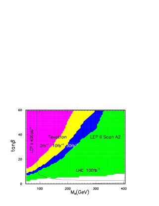
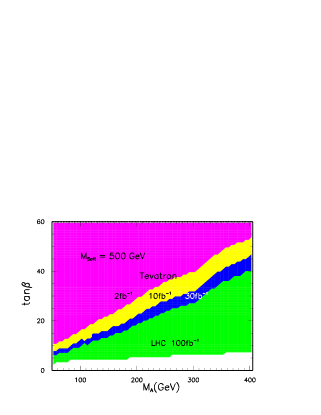
Figure 3: $95\%$ C.L. theoretical estimates of sensitivity contours in the $\tan\beta$-$m_{A}$ planes of the MSSM. The areas above the four boundaries can be excluded by the Tevatron RunII and the LHC; $M_{\rm soft}=500$ GeV (a) and the “LEP II Scan A2” (b) are shown. From Ref. [30].

3.2 QCD corrections to Higgs production in heavy quark fusion

Recently it was proposed that, due to the top-mass enhanced flavor mixing Yukawa coupling of the charm and bottom to charged scalar or pseudoscalar bosons ($\phi^{\pm}$), the $s$-channel partonic process $c\bar{b},\bar{c}b\to\phi^{\pm}$ can be an important mechanism for the production of $\phi^{\pm}$ [36]. This mechanism is also important for $s$-channel neutral scalar production via $b{\bar{b}}$ fusion. In this section, we describe the complete NLO QCD corrections to these processes. The results were originally calculated in Ref. [37], to which we refer for details. The QCD corrections for the SM Higgs production $b\bar{b}\to H$ has been also discussed in Ref. [38]. The overlapping parts of the two calculations are in agreement.

The NLO contributions to the process $b\bar{b}\to\phi^{0}$ contain three parts: (i) the one-loop Yukawa vertex and quark self-energy corrections (Fig. 4b-d); (ii) real gluon emission in $q\bar{q}^{\prime}$ annihilation (Fig. 4e); (iii) $s$- and $t$-channel gluon-quark fusion (Fig. 4f-g). In addition, the renormalization of the fermion–higgs–fermion Yukawa coupling has to be performed. Since the factorization scale $\mu_{F}=m_{\phi}$ is much larger than the mass of the bottom quark, when computing the Wilson coefficient functions the $b$-quarks were treated as massless partons in the proton or anti-proton, similarly to Ref. [39]. The only effect of the heavy quark mass is to determine at which scale $\mu_{F}$ this heavy parton becomes active. (This is the Collins-Wilczek-Zee (CWZ) [40] scheme). The CTEQ4 PDFs [27] are used to calculate the rates, because they are consistent with the scheme used in the current study [41].

Figure 4: Representative diagrams for charged or neutral (pseudo-)scalar (dashed line) production from quark-anti quark and quark-gluon collisions at $O(\alpha_{s}^{0})$ and $O(\alpha_{s}^{1})$: (a) leading order contribution; (b-d) self-energy and vertex corrections (with counter term); (e) real gluon radiation in $q\bar{q^{\prime}}$-fusion; (f-g) $s$- and $t$-channel gluon-quark fusion.

The $\alpha_{s}$ corrections involve the contributions from the emission of real gluons, and as a result the scalar particle will acquire a non-vanishing transverse momentum $Q_{T}$. When the emitted gluons are soft, they generate large logarithmic contributions of the (lowest order) form $\alpha_{s}$$\ln^{m}\left(Q^{2}/Q_{T}^{2}\right)$$/Q_{T}^{2}$, where $Q$ is the invariant mass of the scalar and $m=0,1$. These large logarithms spoil the convergence of the perturbative series, and falsify the $O(\alpha_{s})$ prediction of the transverse momentum when $Q_{T}\ll Q$. To predict the $Q_{T}$ distribution one can use the Collins–Soper–Sterman (CSS) formalism [42], resumming the logarithms of the type $\alpha_{s}^{n}$ $\ln^{m}\left(Q^{2}/Q_{T}^{2}\right)/Q_{T}^{2}$, to all orders $n$ in $\alpha_{s}$ ($m=0,...,2n-1$). The resummation calculation is performed along the same lines as for vector boson production (cf. [43]). To recover the ${\cal O}(\alpha_{s})$ cross section, the Wilson coefficients $C_{i\alpha}^{(1)}$ are included in the resummed calculation in [37]. The non-perturbative sector of the CSS resummation is assumed to be the same as for vector boson production in Ref. [43].

The resummed total rate is the same as the $O(\alpha_{s})$ rate, when we include $C^{(1)}_{i\alpha}$ and the usual fixed order NLO corrections at high $Q_{T}$, and switch from the resummed distribution to the fixed order one at $Q_{T}=Q$. When calculating the total rate, we have applied this matching prescription. In the case of the scalar production, the matching takes place at high $Q_{T}\sim Q$ values, and the above matching prescription is numerically irrelevant when calculating the total rate, since the cross sections around $Q_{T}\sim Q$ are negligible. Thus, as expected, the resummed total rate differs from the $O(\alpha_{s})$ rate only by a few percent. Since the difference of the resummed and fixed order rates and the $K$–factors (c.f. Fig. 6) is small, we can conclude that for inclusive scalar production once the resummation is performed, the $O(\alpha_{s}^{2})$ corrections are likely to be smaller than the uncertainty from the PDF’s.

Figure 5: Cross sections for $A^{0}$ production in the MSSM with $\tan\beta=40$ at the Tevatron and the LHC. (a) The NLO cross sections with the resummed running (solid) and one-loop Yukawa coupling (dashed), as well as the LO cross sections with resummed running (dotted) and tree-level Yukawa coupling (dash-dotted) are shown. The cross sections at $\sqrt{s}=1.8$ TeV (thin set of lowest curves) are multiplied by 0.1 not to overlap with the $\sqrt{s}=2$ TeV curves. (b) The NLO (solid), the $b\bar{b}$ (dashed) and $bg$ (dash-dotted) sub-contributions, and the LO (dotted) contributions. The (negative) $bg$ cross sections are multiplied by $-1$. (c) The NLO cross sections with QCD running Yukawa coupling (solid curves) and those with additional SUSY corrections (top/bottom dashed lines for $\mu=+/-500$ GeV).

Since the QCD corrections are universal, the application to the production of neutral scalar or pseudo-scalar $\phi^{0}$ via the $b\bar{b}$ fusion is straightforward. In the following, we will consider only the production of the pseudo-scalar $A^{0}$ within the context of the MSSM. The total LO and NLO cross sections for the inclusive processes $p\bar{p},pp\to A^{0}X$ at the Tevatron and the LHC are shown in Fig. 5 for $\tan\beta=40$. For other values the cross sections can be obtained by scaling with the factor $(\tan\beta/40)^{2}$.

Fig. 5a shows a significant improvement from the pure LO results (dash-dotted curves) due to the resummation of the large logarithms of $m_{\phi}^{2}/m_{b}^{2}$ into the running coupling. The good agreement between the LO results with running coupling and the NLO results is due to a non-trivial, and process-dependent, cancellation between the individual $O(\alpha_{s})$ contributions of the $b\bar{b}$ and $bg$ sub-processes (which are connected via mass factorization).

Figure 6: The $K$-factors for $A^{0}$ production in the MSSM with $\tan\beta=40$ for the NLO ($K=\sigma_{\rm NLO}/\sigma_{\rm LO}$, solid lines), $b\bar{b}$ ($K=\sigma_{b\bar{b}}/\sigma_{\rm LO}=(\sigma_{\rm LO}+\Delta\sigma_{b\bar{b}})/\sigma_{\rm LO}$, dashed lines), and $bg$ ($K=-\Delta\sigma_{bg}/\sigma_{\rm LO}$, dash-dotted lines) contributions, at the Tevatron (a) and LHC (b).

For large $\tan\beta$, the SUSY correction to the running $\phi^{0}$-$b$-$\bar{b}$ Yukawa coupling can be significant [44], and can be included in a similar way as it is done for the $\phi^{0}b\bar{b}$ associate production [45]. To illustrate the effects of these corrections, all MSSM soft-breaking parameters and $\mu$ were set to $500$ GeV. Depending on the sign of $\mu$, the correction to the coupling can take either the same or opposite sign as the full NLO QCD correction [45]. In Fig. 5c, the solid curves represent the NLO cross sections with QCD correction alone, while the results including the SUSY corrections to the running bottom Yukawa coupling are shown for $\mu=+500$ GeV (top dashed curves) and $\mu=-500$ GeV (bottom dashed curves). These partial SUSY corrections can change the cross sections by about a factor of 2.

Figure 7: The ratios of NLO cross sections computed by four different sets of CTEQ4 PDFs to the cross section computed by CTEQ4M for neutral pseudo-scalar ($A^{0}$) production in the MSSM with $\tan\beta=40$, at the upgraded Tevatron (a) and the LHC (b).

Figure 8: Transverse momentum distributions of pseudo-scalar $A^{0}$ produced via hadron collisions, calculated in the MSSM with $\tan\beta=40$. The resummed (solid) and $O(\alpha_{s})$ (dashed) curves are shown for $m_{A}=$ 200, 250, and 300 GeV at the upgraded Tevatron (a), and for $m_{A}=$ 250, 400, and 550 GeV at the LHC (b).

The $K$-factors, the ratios of the NLO versus LO cross sections as defined in Ref. [37], for the $p\bar{p},pp\to A^{0}X$ processes are presented in Fig. 6 for the MSSM with $\tan\beta=40$. Depending on the $A^{0}$ mass, they range from about $-(16$$\sim$17)% to +5% at the Tevatron and the LHC. The uncertainties of the CTEQ4 PDFs for $A^{0}$-production at the Tevatron and the LHC are summarized in Fig. 7.

The transverse momentum distributions of $A^{0}$, produced at the upgraded Tevatron and at the LHC, are shown in Fig. 8 for various $A^{0}$ masses with $\tan\beta=40$. The solid curves are the result of the multiple soft-gluon resummation, and the dashed ones are from the $O(\alpha_{s})$ calculation. The fixed order distributions are singular as $Q_{T}\to 0$, while the resummed ones have a maximum at some finite $Q_{T}$, and vanish at $Q_{T}=0$. When $Q_{T}$ becomes large, of the order of $m_{A}$, the resummed curves merge into the fixed order ones. The average resummed $Q_{T}$ varies between 25 and 30 (40 and 60) GeV in the 200 to 300 (250 to 550) GeV mass range of $m_{A}$ at the Tevatron (LHC).

In summary, the overall NLO corrections to the $p\bar{p},pp\to A^{0}X$ processes are found to vary between $-(16$$\sim$17)% and +5% at the Tevatron and the LHC in the relevant range of the $A^{0}$ mass. The uncertainties of the NLO rates due to the different PDFs also have been systematically examined, and found to be around $20\%$. The QCD resummation, including the effects of multiple soft-gluon radiation, was also performed to provide a better prediction of the transverse momentum distribution of the scalar $\phi^{0}$. This latter is important when extracting the experimental signals. Similar results can be easily obtained for the other neutral higgs bosons ($h^{0}$ and $H^{0}$) by properly rescaling the coupling. These QCD corrections can also be applied to the generic two higgs-doublet model (called type-III 2HDM[46]), in which the two higgs doublets $\Phi_{1}$ and $\Phi_{2}$ couple to both up- and down-type quarks.

4 Higgs search in the $\gamma\gamma$+jet channel at LHC

The observation of a Higgs boson with a mass $M_{H}<140$ GeV at the LHC in the inclusive channel $pp\to\gamma\gamma+X$ is not easy [47, 48] as it is necessary to separate a rather elusive Higgs boson signal from the continuum background. In Ref. [49] the reaction $pp\to H(\to\gamma\gamma)$+jet, when the Higgs boson is produced with large transverse momentum recoiling against a hard jet, was analyzed as a discovery channel. The signal rate is much smaller, but there remains enough events to discover the Higgs boson at a low luminosity LHC. It is important to note that the situation with the background is undoubtedly much better in the case of Higgs production at high $p_{T}$. Thus, one has $S/B\sim 1/2-1/3$ for CMS and ATLAS correspondingly, providing a discovery significance of 5 already with an integrated luminosity of 30 fb^-1. Furthermore, recent achievements in calculations of QCD next–to–leading corrections have shown an enhancement of the signal against the background. This circumstance together with the possibility to exploit the event kinematics in a more efficient way allow the hope that this reaction will be the most reliable discovery channel for Higgs bosons with masses $M_{H}=110-135$ GeV.

Typical acceptances of the LHC detectors ATLAS and CMS were taken into account in the analysis: two photons are required with $p_{t}^{\gamma}>40$ GeV for each photon (harder than for the inclusive channel), and $|\eta_{\gamma}|<2.5$, while a jet was required with $E_{t}^{jet}>30$ GeV and $|\eta_{jet}|<4.5$, thus involving the forward parts of the hadronic calorimeter. The isolation cut $\Delta R>0.3$ was applied for each $\gamma\gamma$ and $\gamma g(q)$ pair.

There are three QCD subprocesses giving a signal from the Higgs boson in the channel under discussion in QCD leading order: $gg\to H+g$, $gq\to H+q$ and $q\bar{q}\to H+g$. It was found that the $gg\to H+g\to\gamma\gamma+g$ subprocess gives the main contribution to the signal rate. In total, the QCD signal subprocesses give 5.5, 10.6 and 9.8 fb for $M_{H}=100$, 120 and 140 GeV, correspondingly within the kinematical cuts described above.

Another group of signal subprocesses includes the electroweak reactions of Higgs production through $WW$ or $ZZ$ fusion and in association with $W$ or $Z$ boson, where one should veto the second quark jet. The EW signal rate is at the level of 10% of the QCD signal.

Both the reducible and irreducible backgrounds, $pp\to\gamma\gamma$+jet have been discussed in the QCD section of these Proceedings. It was found that in total it is about 19, 31 and 32 fb in the 1 GeV bin for $M_{H}=100$, 120 and 140 GeV, correspondingly.

Further improvement of the $S/B$ ratio can be obtained by studying the kinematical distributions of the 3–body final states in the subprocesses under discussion. The background processes contribute at a smaller $\sqrt{\hat{s}}$ in comparison to the QCD signal processes. So, the corresponding cut improves the S/B ratio: e.g., the cut $\sqrt{\hat{s}}>300$ GeV suppresses the background by a factor of 8.7 while the QCD signal is suppressed only by a factor of 2.6. This effect is connected with the different shapes, Fig. 9, of the jet angular distributions in the partonic c.m.s. for the signal and background. Indeed, for the dominant signal subprocess $gg\to H+g$, a set of possible in spin states does not include spin 1, while the spin of the out state is determined by the gluon. It means, in particular, that the S–wave does not contribute here. At the same time, in the dominant background subprocesses $gq\to\gamma\gamma+q$ and $q\bar{q}\to\gamma\gamma+g$, the same spin configurations are possible for both in and out states. It was found that the cut on the partonic collision energy $\sqrt{\hat{s}}$ matches this spin-states effect, and the best $S/B$ ratio is obtained at $\sqrt{\hat{s}}>300$ GeV. One can try to exploit this effect to enhance the signal significance with the same level of the $S/B$ ratio. Indeed, if one applies the cut on the angle between the jet and the photon in partonic c.m.s. $\cos{\vartheta_{j-\gamma}^{*}}<-0.87$ for $\sqrt{\hat{s}}<300$ GeV and add such events to the events respecting the only cut $\sqrt{\hat{s}}>300$ GeV, then the $S/B$ change is rather small, while the significance is improved by a factor of about 1.3. The same effect can be observed with the cut on the jet production angle in the partonic c.m.s. $\vartheta_{jet}^{*}$, but one should note that the two variables, $\theta_{j-\gamma}^{*}$ and $\vartheta_{jet}^{*}$, are correlated. It is desirable to perform a multivariable optimization of the event selection.

Note that this is a result of a LO analysis, the task for the next step is to understand how this effect will work in presence of NLO corrections to both the signal and background.

In the analysis performed in Ref. [49] the factor $K^{NLO}=1.6$ was used to take into account the QCD next–to–leading corrections for both the signal and background subprocesses. In Ref. [50, 51, 52], this assumption was confirmed by an accurate evaluation of NLO corrections to the signal subprocesses (where for the evaluation of the two–loop diagrams, the effective point–like vertices were used in the limit $M_{H}\ll m_{t}$ [20]). For the background, the corresponding analysis [53] has shown that the NLO corrections are not larger than 50%. Thus, an attractive feature of the $pp\to H(\to\gamma\gamma)$+jet channel is that theoretical uncertainties related to higher order QCD corrections can be under control.

Figure 9: Distributions in the jet production angle $\vartheta^{*}_{jet}$ and the angle $\vartheta^{*}_{j\gamma}$ between jet and the photon with smaller $p_{T}$ in partonic c.m.s. for the QCD signal (S) and background (B). The Higgs mass is taken to be $M_{H}=120$ GeV. Upper plots – no $\sqrt{\hat{s}}$ cut, in others $\sqrt{\hat{s}}>210$ and 300 GeV correspondingly. The $M_{\gamma\gamma}$ bin is equal to 1 GeV.

1 Introduction

The minimal supersymmetric Standard Model (MSSM) contains two complex Higgs doublets, $\phi_{1}$ and $\phi_{2}$, corresponding to eight scalar states. Three of these are absorbed as Goldstone bosons leaving five physical states – the two neutral scalars $(h^{0},H^{0})$, a pseudo-scalar $(A^{0})$ and a pair of charged Higgs bosons $(H^{\pm})$. All the tree-level masses and couplings of these particles are given in terms of two parameters, $m_{H^{\pm}}$ and $\tan\beta$, the latter representing the ratio of the two vacuum expectation values [1]. While any one of the above neutral Higgs bosons may be hard to distinguish from that of the Standard Model, the $H^{\pm}$ carries a distinctive hall-mark of the SUSY Higgs sector. Moreover the couplings of the $H^{\pm}$ are uniquely related to $\tan\beta$, since the physical charged Higgs boson corresponds to the combination

$$H^{\pm}=-\phi^{\pm}_{1}\sin\beta+\phi^{\pm}_{2}\cos\beta.$$ (1)

Therefore the detection of $H^{\pm}$ and measurement of its mass and couplings are expected to play a very important role in probing the SUSY Higgs sector.

The search for charged Higgs bosons is one of the major tasks of present and future high–energy colliders. In a model independent way, LEP2 has set a lower limit on the $H^{\pm}$ mass, $m_{H^{\pm}}\raisebox{-3.69899pt}{~{}\shortstack{$>$ \\ [-0.07cm] $\sim$}}~{}74$ GeV, for any value of $\tan\beta$ [2]. At the Tevatron, the CDF and DØ collaborations searched for $H^{\pm}$ bosons in top decays through the process $p\bar{p}\rightarrow t\bar{t}$, with at least one of the top quarks decaying via $t\rightarrow H^{\pm}b$, leading to a surplus of $\tau$’s due to the $H^{\pm}\to\tau\nu$ decay; they excluded the low and high $\tan\beta$ regions [where the branching ratios for this decay is large] almost up to the $M_{H^{\pm}}\sim m_{t}$ limit [3]. Detailed analyses at the LHC have shown that the entire range of $\tan\beta$ values should be covered for $M_{H^{\pm}}\raisebox{-3.69899pt}{~{}\shortstack{$<$ \\ [-0.07cm] $\sim$}}~{}m_{t}$ [4] using this process.

At this workshop, we focused on the large mass region, $M_{H^{\pm}}>m_{t}$, where the previous production process is not at work and for which only a few preliminary studies have been performed. We summarize our work in this contribution. After a brief summary of the $H^{\pm}$ decay modes [both in the MSSM and in some of its extensions], we will discuss in section 3, the various signals for a heavy charged Higgs boson at the LHC. We will then present, in sections 4 and 5, two simulations for the detection of the $H^{\pm}$ signals in the decay channels $H^{\pm}\to\tau^{\pm}\nu$ in the CMS and $H^{\pm}\to cs,W^{\pm}h,tb$ in the ATLAS detectors.

2 Production and decay modes of the $H^{\pm}$ bosons

The decays of the charged Higgs bosons are in general controlled by their Yukawa couplings to up– and down–type fermions $u,d$ given by [1]:

$${gV_{ij}\over\sqrt{2}M_{W}}H^{+}\left[\cot\beta\;m_{u}\;\bar{u}_{i}d_{jL}+\tan\beta\;m_{d}\;\bar{u}_{i}d_{jR}\right],$$ (2)

For values $\tan\beta>1$, as is the case in the MSSM, the couplings to down–type fermions are enhanced. The coupling $H^{-}tb$, which is of utmost importance in the production and the decays of the $H^{\pm}$ bosons, is large for $\tan\beta\sim 1$ and $\sim m_{t}/m_{b}$. Interestingly these two regions of $\tan\beta$ are favored by $b$–$\tau$ unification for a related reason: i.e. one needs a large $tbH^{\pm}$ Yukawa coupling contribution to the RGE to control the rise of $m_{b}$ as one goes down from the GUT to the low energy scale [8].

Figure 1: Branching ratios of the charged Higgs boson decays for $\tan\beta=2$ and 30. They are obtained using the program HDECAY [10].

The value of $\tan\beta$ determines to a large extent the decay pattern [9] of the charged Higgs bosons. For large $\tan\beta$ values the pattern is simple, a result of the strong enhancement of the couplings to down–type fermions: below the top–bottom threshold, $H^{\pm}$ bosons will decay into $\tau\nu_{\tau}$ pairs while above this threshold, they will decay into $tb$ pairs with BR $\sim 85\%$ and $\tau\nu_{\tau}$ pairs with BR $\sim 15\%$ for large enough $M_{H^{\pm}}$ values. For small $\tan\beta$ values, $\tan\beta\raisebox{-3.69899pt}{~{}\shortstack{$<$ \\ [-0.07cm] $\sim$}}~{}5$, the pattern is more complicated, in particular around and below the $tb$ threshold. Decays into $Wh$ final states play an important role since they reach the level of several ten percent leading to a significant reduction of the dominant branching ratio into $\tau\nu$ states. Note that the off–shell three body decays [9] $H^{\pm}\to bt^{*}\to b\bar{b}W^{\pm}$ and $H^{\pm}\to hW^{*},AW^{*}\to hf\bar{f},Af\bar{f}$ [the latter being kinematically forbidden at the two–body level] can be rather important. The $H^{\pm}$ branching ratios are summarized in Fig. 1 for the values $\tan\beta=2$ and 30.

In the MSSM, the charged and pseudoscalar Higgs boson masses are related [1],

$$M_{H^{\pm}}^{2}=M_{A}^{2}+M_{W}^{2}$$ (3)

and the LEP limit on the lightest scalar and pseudoscalar Higgs masses, $m_{h_{0}}(m_{A_{0}})\raisebox{-3.69899pt}{~{}\shortstack{$>$ \\ [-0.07cm] $\sim$}}~{}90-100~{}{\rm GeV}$ implies first, that $M_{H^{\pm}}\raisebox{-3.69899pt}{~{}\shortstack{$>$ \\ [-0.07cm] $\sim$}}~{}120$ GeV $[M_{H^{\pm}}\raisebox{-3.69899pt}{~{}\shortstack{$>$ \\ [-0.07cm] $\sim$}}~{}200$ GeV for $\tan\beta=2$] and second, that the $H^{\pm}\rightarrow Wh^{0}(WA^{0})$ decay channel has as high a threshold as the $t\bar{b}$ channel, while the latter has a more favorable coupling. Consequently the $H^{\pm}\rightarrow Wh^{0}(WA^{0})$ decay $BR$ is restricted to be $\raisebox{-3.69899pt}{~{}\shortstack{$<$ \\ [-0.07cm] $\sim$}}~{}5\%$ over the LEP allowed region [Fig. 1]. However the constraints discussed above do not hold in singlet extensions of the MSSM like the NMSSM [11]. Consequently $H^{\pm}\rightarrow Wh^{0}(WA^{0})$ can be the dominant decay mode for $M_{H^{\pm}}\sim 160~{}{\rm GeV}$ in the low $\tan\beta$ region and lead to a spectacular signal at the LHC, as illustrated in Table 1. This decay channel will be analyzed in detail in the next sections.

Table 1. Maximal branching fractions for $H^{\pm}\rightarrow W(h^{0}_{1},A^{0}_{1})$ decay in the NMSSM for fixed input values of $\tan\beta$ and output $H^{\pm}$ mass of $\sim 160$ GeV. The values of the $h^{0}_{1},A^{0}_{1}$ masses and branching fractions are shown along with the corresponding model parameters. Also shown are the $t\rightarrow bH^{\pm}$ branching fraction and the size of the resulting $H^{\pm}\rightarrow W(h^{0}_{1},A^{0}_{1})$ decay signal at LHC.

$$\tan\beta$$

(GeV) (%) (GeV) (GeV) (GeV) (%) (fb)

164 0.4 147 .39,–.25 –158,–59 56,36 51,43 2

2

160 0.8 273 .40,–.73 12, 8 115,15 0,97 –

231 .21,–.41 –101,111 51,137 86,0 2.2

2.5 160 0.5

278 .33,–.72 16,8 113,15 0,95 –

196 .14,–.33 –184,–8 54,27 69,16 1.6

3 160 0.4

341 .22,–.62 23, 6 110,19 0,90 –

An important point which should be mentioned, is that in most of the analyses of the $H^{\pm}$ signals, it is always assumed that it decays only into standard particles and that the SUSY decay modes are shut. But for large values of $M_{H^{\pm}}$, at least the decays into the lightest neutralinos and charginos [and possibly into light sleptons and $\tilde{t},\tilde{b}$ squarks] can be kinematically allowed. These modes could have large decays widths, and could thus suppress the $H^{\pm}\rightarrow tb$ branching ratio in a drastic way [12].

In Fig. 2, the branching fraction BR$(H^{\pm}\to\chi^{0}_{i}\chi_{j}^{\pm}$) [with $i=$1–4 and $j$=1–2] are shown as function of $M_{H^{\pm}}$ for the four values $\tan\beta=2,5,10$ and 30. The choice of the gaugino and higgsino mass parameters $M_{2}=\mu=200$ GeV has been made leading to the lightest chargino and neutralino masses $m_{\chi_{1}^{0}}\sim 80$–90 GeV and $m_{\chi_{1}^{+}}\sim$ 125–150 GeV depending on the value of $\tan\beta$ [small masses are obtained with small $\tan\beta$ input]. The values of the scalar masses are such that sleptons and squarks are too heavy to appear in the decay products of the $H^{\pm}$ boson. As can be seen, for small and large values of $\tan\beta$, the $H^{\pm}tb$ couplings are enhanced and the chargino/neutralino decays are important only for large $H^{\pm}$ masses where many $\chi_{i}^{0}\chi_{j}^{0}$ channels are open. For intermediate $\tan\beta$ values, the $H^{\pm}tb$ Yukawa couplings are suppressed, and the chargino/neutralino decays are dominant for charged Higgs boson masses of a few hundred GeV.

In scenarii where sleptons and squarks [in particular stop and sbottom squarks] are also light, $H^{\pm}$ bosons decays into these states might be kinematically possible as well and would be dominant. This will again suppress in a dramatic way the branching ratio for the $H^{\pm}\to tb$ signature [12]. These SUSY decays, although discussed in the literature, have not been analyzed experimentally up to now. They should, however, not be overlooked for heavy charged Higgs bosons, as they might jeopardize the detection of these particles at the LHC.

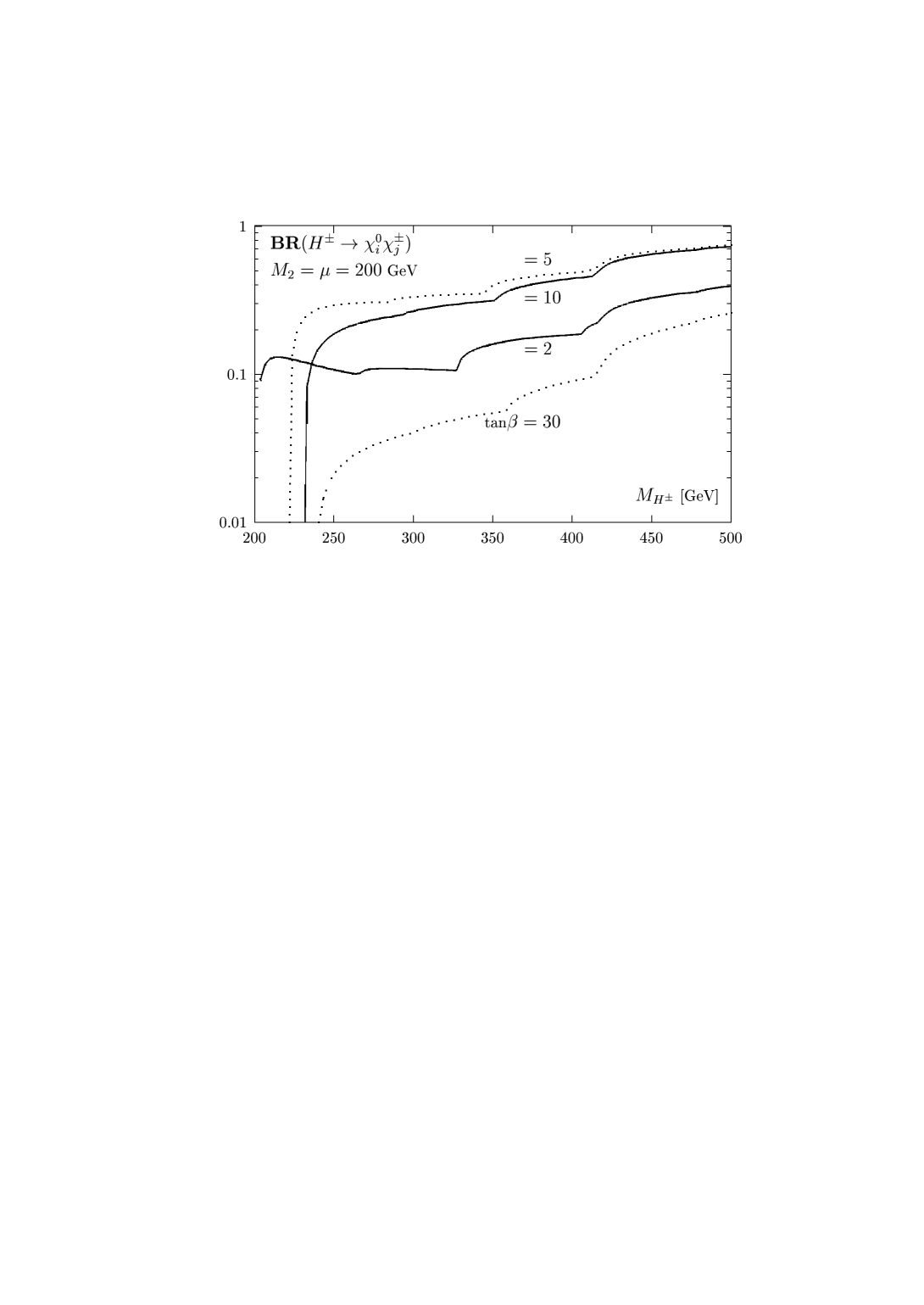
Figure 2: Branching ratios of the charged Higgs boson decays into charginos and neutralinos as a function of $M_{H^{\pm}}$ for a set of $\tan\beta$ values; $M_{2}$ and $\mu$ are fixed to 200 GeV.

Finally, we briefly discuss the production modes of a heavy charged Higgs boson, with $m_{H^{\pm}}>m_{t}$, at the LHC. The two mechanisms which have sizeable cross sections are:

$$pp\to gb(g\bar{b})\to tH^{-}\;(\bar{t}H^{+})$$ [13, 14]

$$pp\to gg/qq^{\prime}\to tH^{-}\bar{b}+\bar{t}H^{+}b$$ [15, 16, 17] (4)

The signal cross-section from the $2\to 2$ mechanism $gb\to tH^{-}$ [where the $b$ quark is obtained from the proton] is 2–3 times larger than the $2\to 3$ process $gg/qq\to t\bar{b}H^{-}$ [where the $H^{-}$ boson is radiated from a heavy quark line]. This is shown in Fig. 3a at LHC energies for the values $\tan\beta=2$ and 40. When the decays $H^{-}\to t\bar{b}$ and $t\to Wb$ take place, the first process gives rise to 3 $b$–quarks in the final state while the second one gives 4 $b$–quarks. Both processes contribute to the inclusive production where at most 3 final $b$–quarks are tagged. However, the two processes have to be properly combined [18] to avoid double counting of the contribution where a gluon gives rise to a $b\bar{b}$ pair that is collinear to the initial proton. The cross section of the inclusive process in this case is shown in Fig. 3b, and is mid–way between the two cross sections eqs. (4) [16].

- -

Figure 3: Production cross sections for charged Higgs bosons at the LHC for $\tan\beta=2$ and 40. (a) Individual cross sections from the $gg/qq$ and $gb$ processes and (b) combination of the two processes with the subtraction of the common piece.

Other mechanisms for $H^{\pm}$ production at hadron colliders are the Drell–Yan type process for pair production, $qq\to H^{+}H^{-}$, the associated production process with $W$ bosons, $qq\to H^{\pm}W^{\mp}$ [19] and the gluon–gluon fusion process for pair production, $gg\to H^{+}H^{-}$ [20]. However, the rates are rather small at the LHC, in the first case because of the weak couplings and the low quark luminosities at high energies and in the second case because the process is induced by loops of heavy quarks and is thus suppressed by additional electroweak coupling factors. We will thus focus in this study on the two processes eq. (4).

3 Signatures of $H^{\pm}$ bosons at the LHC

The $t\rightarrow bH^{+}$ decay is known to provide a promising signature for charged Higgs boson search at the LHC for $M_{H}<m_{t}$. But it is hard to extend the $H^{\pm}$ search beyond $m_{t}$, because in this case the combination of dominant production and decay channel, $tH^{-}\rightarrow t\bar{t}b$, suffers from a large QCD background [14, 15]. Moreover the subdominant production channels of $H^{\pm}W^{\mp}$ and $H^{\pm}H^{\mp}$ have been found to give no viable signature at LHC [19]. In view of this we have undertaken a systematic study of a heavy $H^{\pm}$ signature at the LHC from its dominant production channel $gb(g\bar{b})\to tH^{-}(\bar{t}H^{+})$, followed by the decays $H^{-}\rightarrow\bar{t}b,\tau\bar{\nu}$ and $W^{-}h^{0}$. While the first decay represents the dominant channel of charged Higgs bosons, the $\tau\nu$ and $Wh^{0}$ are the largest subdominant channels in the high and low $\tan\beta$ regions respectively, with [see also Fig. 1]

$$B_{\tau\nu}(\tan\beta\raisebox{-3.69899pt}{~{}\shortstack{$>$ \\ [-0.07cm] $\sim$}}~{}10)\sim 15\%~{}~{}{\rm and}~{}~{}B_{Wh^{0}}(\tan\beta=1-5)\raisebox{-3.69899pt}{~{}\shortstack{$<$ \\ [-0.07cm] $\sim$}}~{}5\%.$$ (5)

The signature for the dominant decay channel of $H^{-}\rightarrow\bar{t}b$ has been analyzed separately assuming three and four $b$–jet tags. The analyses presented in this section are based on parton level Monte Carlo programs with a Gaussian smearing of lepton and jet momenta for simulating the detector resolution.

(i) $H^{\pm}\rightarrow tb$ Signature with Four $b$-tags [17]:

The dominant signal and background processes are

$$gg\rightarrow tH^{-}\bar{b}+{\rm h.c.}\rightarrow t\bar{t}b\bar{b},$$ (6)

$$gg\rightarrow t\bar{t}b\bar{b},$$ (7)

followed by the leptonic decay of one top and hadronic decay of the other, i.e.

$$t\bar{t}b\bar{b}\rightarrow b\bar{b}b\bar{b}W^{+}W^{-}\rightarrow b\bar{b}b\bar{b}\ell\nu q\bar{q}.$$ (8)

A basic set of kinematic and isolation cuts,

$$p_{T}>20~{}{\rm GeV},~{}|\eta|<2.5,~{}\Delta R=\left[(\Delta\phi)^{2}+(\Delta\eta)^{2}\right]^{1/2}>0.4$$ (9)

is imposed on all the jet and lepton momenta. The $p_{T}$ cut is also imposed on the missing-$p_{T}$, obtained by vector addition of the $p_{T}$’s after resolution smearing. This is followed by the mass reconstruction of the $W$ and the top quark pair, so that one can identify the pair of $b$-jets accompanying the latter. While the harder of these two $b$-jets $(b_{1})$ comes from $H^{\pm}$ decay in the signal, both of them come mainly from gluon splitting in the background. Consequently the $S/B$ ratio is improved by imposing the following cuts on this $b$-jet pair:

$$M_{bb}>120~{}{\rm GeV},~{}E_{b_{1}}>120~{}{\rm GeV~{}~{}and}~{}~{}\cos\theta_{bb}<0.75.$$ (10)

Then each of this $b$-jet pair is combined with each of the reconstructed pair of top to give 4 entries for the invariant mass $M_{tb}$ per event. One of these 4 entries corresponds to the $H^{\pm}$ mass for the signal event, while the others constitute a combinatorial background. Fig. 4 shows this $tb$ invariant mass distribution for the signal (6) and background (7). The right hand scale corresponds to the cross-section for $\epsilon^{4}_{b}=0.1$ – i.e. an optimistic $b$-tagging efficiency of $\epsilon_{b}=0.56$. Reducing it to a more conservative value of $\epsilon_{b}=0.4$ would reduce both the signal and background by a factor of 4 each.

1. The reconstructed $tb$ invariant mass distribution of the $H^{\pm}$ signal (6) and the QCD background (7) in the isolated lepton plus multi-jet channel with 4 $b$-tags. The scale on the right corresponds to a $b$-tagging efficiency factor $\epsilon^{4}_{b}=0.1$.

Table 2. Number of signal and background events in the 4 $b$-tagged channel per $100~{}{\rm fb}^{-1}$ luminosity in a mass window of $M_{H^{\pm}}\pm 40~{}{\rm GeV}$ at $\tan\beta=40~{}(\epsilon_{b}=0.4)$.

$$M_{H^{\pm}}({\rm GeV})$$

310 32.7 26.9 6.3

407 22.7 17.3 5.5

506 13.2  9.9 4.2

605  7.5  5.5 3.2

Table 2 lists the number of signal and background events for a typical annual luminosity of $100~{}{\rm fb}^{-1}$, expected from the high luminosity LHC run, assuming $\epsilon_{b}=0.4$. While the $S/B$ ratio is $>1$, the viability of the signal is limited by the signal size. One expects a $>3\sigma$ signal up to $M_{H^{\pm}}=600~{}{\rm GeV}$ at $\tan\beta=40$. The signal size is very similar at $\tan\beta=1.5$, but smaller in between [the signal process (6) is controlled by the $tbH^{\pm}$ Yukawa coupling, eq. (2), which is large for $\tan\beta\sim 1$ and $\sim m_{t}/m_{b}$, as discussed previously].

(ii) $H^{\pm}\rightarrow tb$ Signature with Three $b$-tags [21]:

The contributions to this signal come from (6) as well as

$$gb\rightarrow tH^{-}+{\rm h.c.}\rightarrow t\bar{t}b+{\rm h.c.},$$ (11)

followed by the leptonic decay of one top and hadronic decay of the other. The signal cross-section from (11) is 2–3 times larger than from (6) [Fig. 3], while their kinematic distributions are very similar. Combining the two cross sections and subtracting the overlapping piece to avoid double counting results in a signal cross-section, which is mid–way between the two; see Fig. 3.

The background comes from (7) as well as

$$gb\rightarrow t\bar{t}b+{\rm h.c.}~{}~{}{\rm and}~{}~{}gg\rightarrow t\bar{t}g,$$ (12)

where the gluon jet in the last case is mis-tagged as a $b$-jet. Assuming the standard mis-tagging factor of 1% this contribution turns out in fact to be the largest source of the background, as we see below.

The basic kinematic cuts are as in (9) except for a harder $p_{T}$-cut,

$$p_{T}>30~{}{\rm GeV},$$ (13)

since the 3 $b$-jets coming from $H^{\pm}$ and $t\bar{t}$ decays are all reasonably hard. This is followed by the mass reconstruction of the top quark pair as before, so that one can identify the accompanying (3rd) $b$-jet. We impose a

$$p_{T}>80~{}{\rm GeV}$$ (14)

cut on this $b$-jet to improve the $S/B$ ratio. Finally this $b$-jet is combined with each of the reconstructed top pair to give two entries of $M_{tb}$ per event. One of them corresponds to the $H^{\pm}$ mass for the signal while the other constitutes the combinatorial background. Fig. 5 shows this $tb$ invariant mass distribution of the signal along with the above mentioned backgrounds, including a $b$-tagging efficiency factor of

$$\epsilon_{b}=0.4.$$ (15)

While the $S/B$ ratio is $<1$ the signal cross-section is much larger than the previous case. Table 3 lists the number of signal and background events for a luminosity of $100~{}{\rm fb}^{-1}$ at $\tan\beta=40$. The results are very similar at $\tan\beta=1.5$. Comparing this with Table 2 we see that the $S/\sqrt{B}$ ratio is very similar in the two channels. One should bear in mind however the larger $p_{T}$ cut (13) assumed for the 3 $b$-tagged channel. The cross-sections in both the cases were calculated with the MRS-LO structure functions [22].

1. The reconstructed $tb$ invariant mass distribution of the $H^{\pm}$ signal and different QCD backgrounds in the isolated lepton plus multi-jet channel with 3 $b$-tags.

Table 3. Number of signal and background events in the 3 $b$-tagged channel per $100~{}{\rm fb}^{-1}$ luminosity in a mass window of $M_{H^{\pm}}\pm 40~{}{\rm GeV}$ at $\tan\beta=40~{}(\epsilon_{b}=0.4)$.

$$M_{H^{\pm}}~{}({\rm GeV})$$

310 133 443 6.2

407 111 403 5.6

506  73 266 4.5

605  43 156 3.4

(iii) $H^{\pm}\rightarrow\tau\nu$ Signature [23]:

Following the analysis of Ref. [23] a more exact simulation of a heavy $H^{\pm}$ signature in the $\tau\nu$ decay channel was done for the CMS detector using PYTHIA [24]. The results will be presented in the next section. By exploiting the distinctive $\tau$ polarization one can get at least as good a $H^{\pm}$ signature here as in the $t\bar{b}$ channel for the large $\tan\beta$ region.

(iv) $H^{\pm}\rightarrow W^{\pm}h^{0}$ Signature [25]:

For simplicity we have estimated the signal cross-section from

$$gb\rightarrow tH^{-}+{\rm h.c.}\rightarrow bW^{+}W^{-}h^{0}+{\rm h.c.},$$ (16)

followed by $h^{0}\rightarrow b\bar{b}$, $W^{\pm}\rightarrow\ell\nu$ and $W^{\mp}\rightarrow q\bar{q}$. Thus the final state consists of the same particles as the dominant decay mode of eq. (11). Thus we have to consider the background from the $H^{-}\rightarrow t\bar{b}$ decay (11) along with those from the QCD processes of eq. (12).

We require 3 $b$-tags along with the same basic cuts as in section (ii). This is followed by the mass reconstruction of $W^{\pm}$ and the top, which helps to identify the accompanying $b$-pair and the $W$. The resulting $bb$ and $Wb$ invariant masses are then subjected to the constraints,

$$M_{bb}=m_{h^{0}}\pm 10~{}{\rm GeV}~{}{\rm and}~{}m_{Wb}\neq m_{t}\pm 20~{}{\rm GeV}.$$ (17)

The $h^{0}$ mass constraint and the veto on the second top helps to separate the $H^{\pm}\rightarrow W^{\pm}h^{0}$ signal from the backgrounds. However the former is severely constrained by the signal size as well as the $S/B$ ratio. Consequently one expects at best a marginal signal in this channel and only in a narrow strip of the $M_{H^{\pm}}$–$\tan\beta$ parameter space, at the boundary of the LEP exclusion region. Fig. 6 shows the signal (16) along with the backgrounds from (11) and (12) against the reconstructed $H^{\pm}$ mass at one such point – $M_{H^{\pm}}=220~{}{\rm GeV}$ and $\tan\beta=2$. Note that, as discussed in section 2, in extensions of the MSSM, the $H^{\pm}\rightarrow Wh^{0}(WA^{0})$ can be the dominant decay mode for $M_{H^{\pm}}\sim 160~{}{\rm GeV}$ in the low $\tan\beta$ region and lead to a spectacular signal at the LHC; see Table 1.

Fig. 6 The $H^{\pm}\rightarrow Wh^{0}$ signal cross-section is shown against the reconstructed $H^{\pm}$ mass for $M_{H^{\pm}}=220~{}{\rm GeV}$ and $\tan\beta=2$ along with the $H^{\pm}\rightarrow tb$ and the QCD backgrounds.

It should be mentioned here that these parton level Monte Carlo analyses of the $H^{\pm}$ signature in $tb$ and $Wh^{0}$ decay channels need to be followed up by detailed simulation with PYTHIA, including detector acceptance, as in the case of the $\tau\nu$ channel discussed in the next section. Some work has started here along this line for the ATLAS detector; this is summarized in section 5. One should also bear in mind the possibility of large radiative corrections to the Yukawa coupling eq. (2); it is evidently important to include these corrections for a quantitative evaluation of this signal.

4 The $H^{+}\rightarrow\tau\nu$ mode in CMS

4.1 Introduction

As mentioned in the previous section, the hadronic $\tau$ signature of a heavy charged Higgs boson from $pp\rightarrow tH^{\pm}$ at the LHC is useful. In this contribution, we study the search of heavy $H^{\pm}$ bosons in the CMS detector with a realistic simulation using the procedure of Ref. [23] to select the events and to exploit the $\tau$ polarization effects. The main backgrounds are due to $t\overline{t}$ and $W$+jet events. The $W$+jet background can be effectively reduced with $W$ and top mass reconstruction and $b$–tagging. Although for $t\overline{t}$ and $W$+jet events the transverse mass reconstructed from the $\tau$–jet and the missing transverse energy is bounded from above by the $W$ mass, some leaking of the backgrounds into the signal region can be expected due to the experimental resolution of the $E_{t}^{miss}$ measurement.

4.2 Event selection and expectations for CMS

Events are generated with PYTHIA [24] using the process $bg\rightarrow tH^{\pm}$. The results from Ref. [21] with a subtraction of double counting between the $g\overline{b}\rightarrow\overline{t}H^{\pm}$ and $gg\rightarrow\overline{t}bH^{\pm}$ processes are used to normalize the PYTHIA cross sections. The $H^{\pm}\rightarrow\tau\nu$ branching ratio is calculated with the HDECAY program [10] and used in the simulation. A heavy SUSY particle spectrum (1 TeV) is assumed with no stop mixing. The decay matrix elements with polarization effects [23, 26] are added in PYTHIA. For $m_{H^{\pm}}$ = 400 GeV and $\tan\beta$ = 40 about 1700 signal events, including only one-prong hadronic $\tau$ decays, are expected for an integrated luminosity of 30 fb^-1. The jets and the missing transverse energy are reconstructed with a fast simulation package CMSJET [27]. For b-tagging, results obtained from a full simulation and reconstruction of the CMS tracker are used [28].

The real $\tau$ jet is chosen as the $\tau$ jet candidate requiring $E_{t}>$ 100 GeV and $|\eta|<$2.5. The events can be triggered with a multi-jet trigger and a higher level $\tau$ trigger even in the high luminosity running conditions. The $\tau$ selection is performed here using only the tracker information. The algorithm of ref. [23] to remove the transverse components of the $\tau$ polarization is used requiring r = $p^{\pi}$ / $E^{\tau jet}>$ 0.8, where $p^{\pi}$ is the momentum of a hard pion from $\tau$ decay in a cone of $\Delta R<$ 0.1 around the calorimeter jet axis and $E^{\tau jet}$ is the hadronic energy of the $\tau$ jet ($E_{t}>$ 100 GeV) reconstructed in the calorimeters (electromagnetic and hadronic) in a cone of $\Delta R<$ 0.4. The efficiency of this $\tau$ selection for the signal events is 20% while for the $t\overline{t}$ events the efficiency is only 0.4% (including the $E_{t}$ threshold for jet). A reconstruction efficiency of 95% is assumed for the hard isolated track from $\tau$.

A large missing transverse energy is expected in the signal events due to the neutrino from $H^{\pm}$ decay. The $E_{t}^{miss}$ is reconstructed with the CMSJET package, where the calorimeter response is parametrized including the effects of the detector cracks and the volumes of degraded response. Efficiency of the cut $E_{t}^{miss}>$ 100 GeV is about 75% for the signal events and about 39% for the $t\overline{t}$ background.

A visible signal for the Higgs can be obtained in the transverse mass reconstructed from the $\tau$-jet and the missing transverse energy if the hadronic decay of the associated top quark is selected. For the reconstruction of the $W$ and top masses the events with at least three jets with $E_{t}>$ 20 GeV, in addition to the $\tau$ jet, are selected. The $W$ and top masses are reconstructed minimizing the variable $\chi^{2}$ = $(m_{jj}-m_{W})^{2}+(m_{jjj}-m_{t})^{2}$, where $m_{W}$ and $m_{t}$ are the nominal $W$ and top masses. A Gaussian resolution of 13.6 GeV is found for the reconstructed top mass. The fraction of events where the three jets are found and the reconstructed $W$ mass is within $m_{W}\pm$ 15 GeV and the reconstructed top mass within $m_{t}\pm$ 20 GeV is 54% for the signal, 59% for the $t\overline{t}$ background and 8% for the $W$+jet events.

After the $W$ and top mass reconstruction and the mass window cuts b-tagging is applied on the jet not assigned to the $W$. This jet is required to be harder with $E_{t}^{jet}>$ 30 GeV. The tagging efficiencies based on the impact parameter method obtained from a full simulation and track reconstruction in the CMS tracker are used [28]. At least two tracks with $p_{t}>$ 1 GeV and impact parameter significance $\sigma^{ip}>$ 2 are required inside the jet reconstruction cone of 0.4. For b-jets with $E_{t}$ = 50 GeV the efficiency is found to be $\sim$ 50% averaged over the full $\eta$ range ($|\eta|<2.5$). The mis-tagging rate for the corresponding light quark and gluon jets is 1.3%.

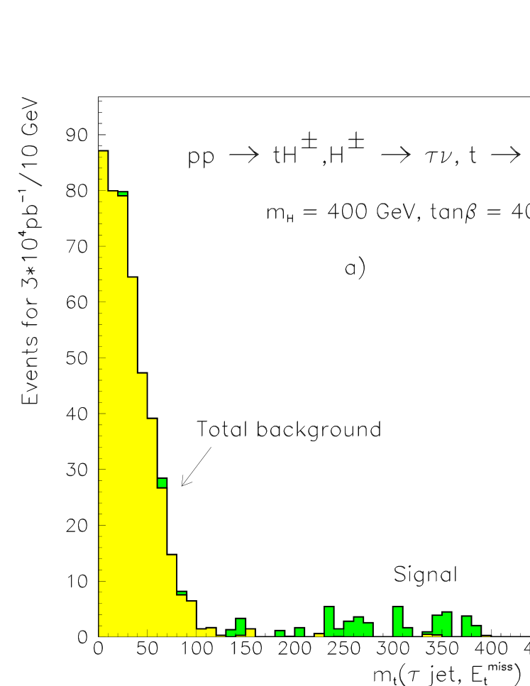
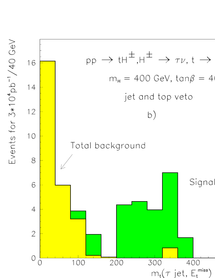
Figure 7: a) Transverse mass reconstructed from $\tau$ jet and $E_{t}^{miss}$ for $H^{\pm}\rightarrow\tau\nu$ from $pp\rightarrow tH^{\pm}$ with $m_{H^{\pm}}$ = 400 GeV and $\tan\beta$ = 40 over the total background from $t\overline{t}$ and $W$+jet events. b) the same as in a) but with a veto on a central jet and a second top.

The reconstructed transverse mass $m_{T}^{\tau\nu}$ over the total background is shown in Fig. 7a for $m_{H^{\pm}}$ = 400 GeV and $\tan\beta$ = 40 for 30 fb^-1. For $m_{T}^{\tau\nu}>$100 GeV about 44 signal events are expected for $m_{H^{\pm}}$ = 400 GeV and $\tan\beta$ = 40 and about 25 events for $m_{H^{\pm}}$ = 200 GeV and $\tan\beta$ = 30, for an integrated luminosity of 30 fb^-1. About 5 background events from $t\overline{t}$ and $W+jet$ are expected for $m_{T}^{\tau\nu}>$100 GeV. Further reduction of the $t\overline{t}$ background is still possible using a jet veto cut and a veto on a second top in the event. Since a soft and a relatively forward spectator b-jet from the production process is expected in the signal events, a central and hard jet veto with $|\eta^{jet}|<$ 2 and $E_{t}^{jet}>$ 50 GeV is used. For the reconstruction of the second top from the $\tau$ jet, missing energy and one of the remaining jets, the longitudinal component of the missing energy is first resolved from the $W$ mass constraint selecting the smaller of the two solutions. The reconstructed top mass is required to fall outside the window of $m_{t}\pm$ 60 GeV. The central jet veto and the second top veto, being closely correlated cuts, reduce $t\overline{t}$ background by a factor of $\sim$7. The efficiency for the signal is 54%. The transverse mass $m_{T}^{\tau\nu}$ distribution over the total background including the jet and second top veto is shown in Fig. 7b for $m_{H^{\pm}}$ = 400 GeV and $\tan\beta$ = 40 and in Fig. 8a for $m_{H^{\pm}}$ = 200 GeV and $\tan\beta$ = 30.

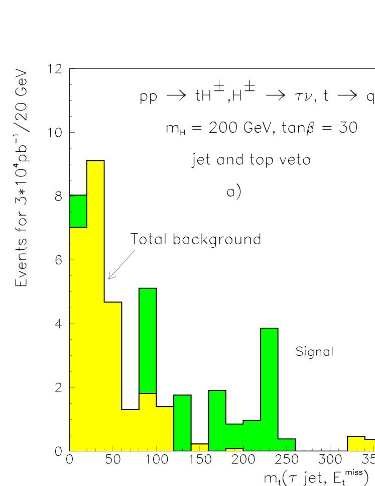
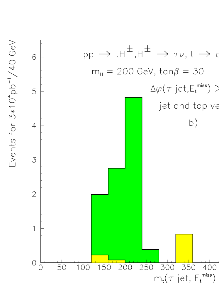
Figure 8: a) Transverse mass reconstructed from $\tau$ jet and $E_{t}^{miss}$ for $H^{\pm}\rightarrow\tau\nu$ from $pp\rightarrow tH^{\pm}$ with $m_{H^{\pm}}$ = 200 GeV and $\tan\beta$ = 30 over the total background from $t\overline{t}$ and $W$+jet events with central jet and second top veto. b) the same as in a) but for $\Delta\phi>50^{o}$ where $\Delta\phi$ is the angle between the $\tau$ jet and the $E_{t}^{miss}$ vector in the transverse plane.

The visibility of the signal can be significantly improved, especially at $m_{H^{\pm}}$ = 200 GeV, with a cut on the $\Delta\phi$ angle between the $\tau$ jet and the $E_{t}^{miss}$. Although $\Delta\phi$ is directly proportional to $m_{T}^{\tau\nu}$, a cut in $\Delta\phi$ suppresses the background efficiently at the lower end of the expected signal region as can be seen from Fig. 8b showing the signal over the total background with $\Delta\phi>50^{o}$ for $m_{H^{\pm}}$= 200 GeV and $\tan\beta$ = 30.

4.3 Conclusion

Our preliminary study leads to the conclusion that $H^{\pm}\rightarrow\tau\nu$ from $pp\rightarrow tH^{\pm}$ is a promising discovery channel for charged Higgs bosons at the LHC. For the evaluation of the final discovery reach in the $m_{A}$, $\tan\beta$ parameter space a detailed simulation of the $E_{t}^{miss}$ measurement for the background events is needed. The study can be extended to high luminosity but some additional loss of efficiency should be expected due to the harder $E_{t}^{jet}$ cuts due to trigger requirements.

5 The $H^{+}\rightarrow cs,Wh,tb$ modes in ATLAS

5.1 Introduction

In this section we describe the charged Higgs boson discovery potential of the ATLAS detector in the ($m_{H^{\pm}}$, $\tan\beta$) parameter space which has been investigated using the ATLFAST [29] and PYTHIA 5.7 [24] simulation packages. This is a particle–level simulation performed at $\sqrt{s}=14$ TeV, but with the detector resolutions and efficiencies parametrized from full detector simulations. It is assumed that the mass scale of supersymmetric partners of ordinary matter is above the charged Higgs bosons so that $H^{\pm}$ decays into supersymmetric partners are forbidden [30]. A central value 175 GeV is used for the top-quark mass.

The decays $H^{\pm}\rightarrow tb$ and $H^{\pm}\rightarrow\tau\nu$ are the dominant channels in most of the parameter space [10]. The decay channel $H^{\pm}\rightarrow\tau\nu$ has been studied extensively for ATLAS for $m_{H^{\pm}}<m_{t}$, and the signal appears as an excess of $\tau$ leptons [31]. The channel $H^{\pm}\rightarrow Wh^{0}$ is only relevant in a tiny range of MSSM parameter space but it constitutes a unique test for MSSM and may be sensitive to the singlet extension to MSSM, i.e., NMSSM. The $H^{\pm}\rightarrow c\bar{s}$ channel is studied as a complement to the $\tau$-lepton channel: if the charged Higgs is detected by observing the excess of $\tau$-leptons over the SM prediction, then the $c\bar{s}$ channel could be used to measure $m_{H^{\pm}}$. Discovery is possible through the $H^{+}\to t\bar{b}$ channel for low $(\raisebox{-3.69899pt}{~{}\shortstack{$<$ \\ [-0.07cm] $\sim$}}~{}3)$ and large $(\raisebox{-3.69899pt}{~{}\shortstack{$>$ \\ [-0.07cm] $\sim$}}~{}25)$ $\tan\beta$ values up to masses $m_{H^{\pm}}\sim 400$ GeV. In the following, a brief description of the analysis is presented; details can be found elsewhere [32, 33].

5.2 $H^{\pm}$ Discovery Potential

(i) $\mathbf{t\rightarrow bH^{\pm}\rightarrow bc\bar{s}}$, $\mathbf{m_{H^{\pm}}<m_{t}}$: $t\bar{t}$ events are generated through $gg,\,q\bar{q}\rightarrow t\bar{t}$ with one top-quark decaying into the charged Higgs, and the other into $W$, $\bar{t}\rightarrow Wb\rightarrow l\nu b$. The major background is $t\bar{t}$ production itself with both top-quark decaying into $W$’s; one of the $W$’s goes to jets and the other to leptons. This process is studied for $\tan\beta=1.5$ and $m_{H^{\pm}}=110$ and 130 GeV. The events with a final state consisting of two b-tagged jets ($|\eta|<2.5$, and $p_{T}>15$ GeV), and a single isolated lepton ($|\eta|<2.5$, $p_{T}^{e}>20$ and $p_{T}^{\mu}>6$ GeV) are selected and the charged mass peak is searched for the di-jet mass distribution $m_{jj}$. The combinatorial background is reduced by applying a b-jet veto and a jet-veto on extra jets. Fig. 9 shows the di-jet mass distribution for both the signal and the background. This channel complements the $H^{\pm}\rightarrow\tau\nu$ channel in that if the $H^{\pm}$ is detected by observing the excess of $\tau$-leptons, the $H^{\pm}\rightarrow c\bar{s}$ channel can be used to determine $m_{H^{\pm}}$.

Figure 9: For the $H^{\pm}\rightarrow cs$ channel, the expected $m_{jj}$ distribution from signal and background events (solid) and from the background (dashed) for $m_{H^{\pm}}=130$ GeV and $\tan\beta=1.5$ and for an integrated luminosity of 30 fb^-1. Errors are statistical only.

(ii) $\mathbf{t\rightarrow bH^{\pm}}$, $\mathbf{H^{\pm}\rightarrow W^{*}h^{0}}$, $\mathbf{m_{H^{\pm}}<m_{t}}$: The production mechanism is the same as in the previous case, but here, $H^{\pm}\rightarrow W^{*}h^{0}$, with $h^{0}\rightarrow b\bar{b}$. The final state contains two $W$’s, one of which is off-shell and one of which decays to leptons and the other to jets. The major backgrounds are $t\bar{t}b\bar{b}$ and $t\bar{t}q\bar{q}$ followed by the decays of the top-quarks as described above. The present channel is studied for $m_{H^{\pm}}=152$ GeV and for $\tan\beta=2$ and 3 corresponding to $m_{h^{0}}=83.5$ and 93.1 GeV respectively. We search for an isolated lepton, four b-tagged jets ($p_{T}^{b}>30$ GeV) and at least two non b-jets with $p_{T}^{j}>30$ GeV. The details of this analysis can be found in [33]. It suffices to say that although the backgrounds are over two orders of magnitude higher that the signal at the start, we propose a reconstruction method which permits the extraction of the signal with a significance exceeding $5\sigma$ in the low $\tan\beta\;(1.5-2.5)$ region. At high $\tan\beta$, though the reconstruction remains comparable the signal rate decreases so significantly that discovery potential vanishes in this region. Fig. 10 shows the charged Higgs mass reconstruction for $\tan\beta=2$.

Figure 10: For the $H^{\pm}\rightarrow W^{*}h^{0}$ channel, the reconstructed mass distribution from signal$+$background events (solid) and from background events (dashed) for $m_{H^{\pm}}=152$ GeV, $\tan\beta=2$, and for and integrated luminosity of 300 fb^-1. Errors are statistical.

(iii) $\mathbf{m_{H^{\pm}}>m_{t}}$: Above the top-quark mass, we consider the production of $H^{\pm}$ through the $2\rightarrow 2$ process $gb\rightarrow tH^{\pm}$. Two decay channels of $H^{\pm}$ are examined in details, $H^{\pm}\rightarrow tb$ and $H^{\pm}\rightarrow Wh^{0}\rightarrow Wb\bar{b}$. In both cases the major background comes from $t\bar{t}b$ and $t\bar{t}q$ events. In either case, we search for an isolated lepton, three b-tagged jets and at least two non b-jets. The details of these analyses can be found elsewhere [32, 33]. Discovery is possible through the $H^{\pm}\rightarrow tb$ channel for low ($<3$) and for high ($>25$) $\tan\beta$ up to $m_{H^{\pm}}\sim 400$ GeV [32]. Fig. 11 shows the charged Higgs mass reconstruction for $\tan\beta=1.5$ and $m_{H^{\pm}}=300$ GeV. On the other hand, the $H^{\pm}\rightarrow Wh^{0}$ channel presents no discovery potential for the charged Higgs in the MSSM. Initially, the total background is at least three orders of magnitude higher than the signal in the most favorable case studied ($\tan\beta=3$). We propose a reconstruction technique which improves the signal-to-background ratios by two orders of magnitude. However, this improvement is still not enough to observe a clear signal; for example, at $\tan\beta=3$, a significance of only 3.3 can be expected after three years of high luminosity operation [33].

Figure 11: Signal and background distributions for the reconstructed invariant mass $m_{tb}$ for $m_{H^{\pm}}=300$ GeV, $\tan\beta=1.5$ and an integrated luminosity of 30 fb^-1. Errors are statistical only.

5.3 Conclusions

The possibility of detecting the charged Higgs through the decay channels $H^{\pm}\rightarrow c\bar{s}$, $H^{\pm}\rightarrow Wh^{0}$, and $H^{\pm}\rightarrow tb$ with the ATLAS detector has been studied as a function of $\tan\beta$, below and above the top-quark mass. Below the top-quark mass and at low $\tan\beta$, both channels $H^{\pm}\rightarrow c\bar{s}$ and $H^{\pm}\rightarrow Wh^{0}$ present significant discovery potential. These two channels would complement the $H^{\pm}\rightarrow\tau\nu$ searches in that if the latter is observed through the excess of $\tau$-leptons, the former channels can be used to measure the mass of the charged Higgs. Above the top-quark mass, the process $H^{\pm}\rightarrow tb$ presents a significant discovery potential in the low and the high $\tan\beta$ regions up to 400 GeV.

Acknowledgements

R.K. would like to thank Daniel Denegri for helpful discussions. K.A.A. expresses gratitude to E. Richter-Wa̧s for fruitful discussions and constructive criticisms; his work is supported by a grant from the USA National Science Foundation (grant number 9722827).

1 Introduction

The third generation fermions, and especially the top quark because of its large Yukawa coupling, play an important rôle in the mechanism of electroweak symmetry breaking and the properties of the Higgs bosons [1]. Recall that if the top quark were rather light, the Minimal Supersymmetric extension of the Standard Model (MSSM) would have been already discarded since the lightest Higgs boson $h$ that it predicts would have been lighter than the $Z$ boson, $M_{h}\leq M_{Z}$ [1], and would have not escaped detection at LEP2. The contribution of the top quark and its SUSY partners to the radiative corrections to $M_{h}$ can push the mass value up to $M_{h}\sim 135$ GeV [2], beyond the reach of LEP2. The mixing in the stop sector is also important since large values of the mixing parameter $\tilde{A}_{t}=A_{t}+\mu/\tan\beta$ [where $A_{t}$ is the trilinear coupling, $\mu$ the higgsino mass parameter and $\tan\beta$ the ratio of the vev’s of the two Higgs doublets which break the electroweak symmetry; see Ref. [3] for the SUSY parameters] can increase the $h$ boson mass for a given value of $\tan\beta$ [2].

On the other hand, while the sfermions of the two first generations can be very heavy, naturalness arguments suggest that the SUSY particles that couple substantially to the Higgs bosons [stops, sbottoms for large $\tan\beta$, and the electroweak gauginos and higgsinos] could be relatively light. In this respect, the case of the stop sector is special: because of the large $m_{t}$ value, the mixing in this sector can be very strong, leading to a mass eigenstate $\tilde{t}_{1}$ lighter that all other squarks, and possibly lighter than the top quark itself. At the same time, again because of the large mixing, this particle can couple very strongly to the MSSM Higgs bosons and in particular to the lightest CP–even particle $h$.

At the LHC, a light stop with large couplings to Higgs bosons can contribute to both the $h$ production in the main channel, the gluon–gluon fusion mechanism $gg\rightarrow h$, and to the main detection channel, the two–photon decay $h\rightarrow\gamma\gamma$. The effects can be extremely large, making this discovery channel possibly useless at the LHC [4–6]. On the other hand, because of the enhanced couplings and phase–space, associated production of stops and the $h$ boson at the LHC, $pp\to q\bar{q}/gg\to\tilde{t}_{1}\tilde{t}_{1}h$, might have sizeable cross sections [7–10].

It is thus crucial to investigate how and when this scenario occurs and what other consequences then follow at the LHC. The purpose of our working group contribution is to update and complement the various analyses [5–10] which have been made on this subject.

2 Stop parameters and phenomenological constraints

We start our discussion by recalling the parameters that define the stop masses, mixing angle and the $\tilde{t}_{1}\tilde{t}_{1}h$ coupling. The stop mass eigenstates are defined through the mixing angle $\theta_{\tilde{t}}$, with the lightest stop $\tilde{t}_{1}$ being $\tilde{t}_{1}=\cos\theta_{\tilde{t}}\;\tilde{t}_{L}-\sin\theta_{\tilde{t}}\;\tilde{t}_{R}$. With the effective trilinear mixing parameter, $\tilde{A}_{t}=A_{t}+\mu/\tan\beta$, one has for the masses and the mixing angle

$$\tan(2\theta_{\tilde{t}})=\frac{-2m_{t}\tilde{A}_{t}}{\tilde{m}_{\tilde{Q}_{3}}^{2}-\tilde{m}_{\tilde{U}_{3R}}^{2}+\frac{1}{2}M_{Z}^{2}\cos 2\beta(1-\frac{8}{3}s_{W}^{2})}\;\;\;\;\;{\rm or}\;\;\;\;\sin(2\theta_{\tilde{t}})=\frac{-2m_{t}\tilde{A}_{t}}{m_{\tilde{t}_{1}}^{2}-m_{\tilde{t}_{2}}^{2}}$$ (1)

$$m_{\tilde{t}_{1,2}}^{2}=m_{t}^{2}+\frac{1}{2}\left[m_{\tilde{Q}_{3}}^{2}+m_{\tilde{U}_{3R}}^{2}+\cdots\mp\sqrt{(m_{\tilde{Q}_{3}}^{2}-m_{\tilde{U}_{3R}}^{2}+\cdots)^{2}+4m_{t}^{2}\tilde{A}_{t}^{2}}\right]\;,$$ (2)

where $m_{\tilde{Q}_{3}}$, $m_{\tilde{U}_{3R}}$ are the soft-SUSY breaking scalar masses and the dots stand for the $D$–terms $\propto M^{2}_{Z}\cos 2\beta$. Note that in order to enhance the mixing, $\sin(2\theta_{\tilde{t}})\sim 1$, one needs to make $\tilde{A}_{t}$ large and/or have the soft-SUSY masses almost equal: $\tilde{m}_{\tilde{Q}_{3}}\simeq\tilde{m}_{\tilde{U}_{3R}}$. The $\tilde{t}_{1}\tilde{t}_{1}h$ vertex writes

$$V_{\tilde{t}_{1}\tilde{t}_{1}h} = -g\frac{m_{t}}{M_{W}}\frac{\cos\alpha}{\sin\beta}\bigg{[}(A_{t}-\mu\tan\alpha)\sin\theta_{\tilde{t}}\;\cos\theta_{\tilde{t}}\;-\;m_{t}$$ (3)

$$+ \frac{M_{Z}^{2}}{m_{t}}\frac{\sin\beta}{\cos\alpha}\sin(\alpha+\beta)\biggr{[}(\frac{1}{2}-\frac{2}{3}\sin^{2}\theta_{W})\cos^{2}\theta_{\tilde{t}}+\frac{2}{3}\sin^{2}\theta_{W}\sin^{2}\theta_{\tilde{t}}\biggr{)}\biggr{]}$$

$$\simeq \frac{g}{M_{W}}\biggr{[}\frac{1}{4}\sin^{2}(2\theta_{\tilde{t}})(m_{\tilde{t}_{1}}^{2}-m_{\tilde{t}_{2}}^{2})\;+\;m_{t}^{2}\biggr{]}$$

where in the last line we neglected the $D$–term contributions and assumed the limit of large $M_{A}$ to be in the decoupling regime. As can be seen, in the presence of large mixing with large splitting between the two stop eigenstates, the $\tilde{t}_{1}\tilde{t}_{1}h$ coupling can be particularly large. In the case of no mixing, only the top contribution survives and the coupling $\tilde{t}_{1}\tilde{t}_{1}h$ is of the order of $t\bar{t}h$ coupling. Taking this limit as a reference point, the strength of the $\tilde{t}_{1}\tilde{t}_{1}h$ vertex can be normalized through $R_{\tilde{t}_{1}}=\left[M_{W}V_{\tilde{t}_{1}\tilde{t}_{1}h}/(gm_{t}^{2})\right]^{2}$.

We now summarize the constraints which can be imposed on the stop parameters:

• The model independent mass limit on the lightest stop is obtained from direct searches at LEP, $m_{\tilde{t}_{1}}\geq 90$ GeV [11]. However, if the $\tilde{t}_{1}$ and the $\chi_{0}$ LSP are not too close in mass, a stronger limit, $m_{\tilde{t}_{1}}\geq 120$ GeV [12], is available from Tevatron analyses. For bottom squarks, a limit $m_{\tilde{b}}\geq 250$ GeV is available from Tevatron data in the case of no–mixing [12].

• If stops are too light, the radiative corrections to the $h$ boson mass are not large enough and the limit $M_{h}\geq 90$ GeV [11] from LEP searches plays an important role.

• As in the case of top/bottom splitting in the Standard Model, the stop/sbottom doublet can contribute significantly to electroweak precision observables through the $\rho$ parameter. In particular, if stops strongly mix and have large couplings, the contributions to $\Delta\rho$ can exceed the value $\Delta\rho\leq 0.0013$ imposed by data [13].

• Some values of the stop parameters might induce color and charge breaking minima (CCB). Since the naive constraints based on the global minima may be too restrictive, we will take into account the tunneling rate [for wide range of parameters, the global CCB minimum becomes irrelevant on the ground that the time required to reach the lowest energy state exceeds the present age of the universe], which leads to a milder constraint which may be approximated by [14]: $A_{t}^{2}+3\mu^{2}<7.5(M_{\tilde{Q}_{3}}^{2}+M_{\tilde{U}_{3R}}^{2})$.

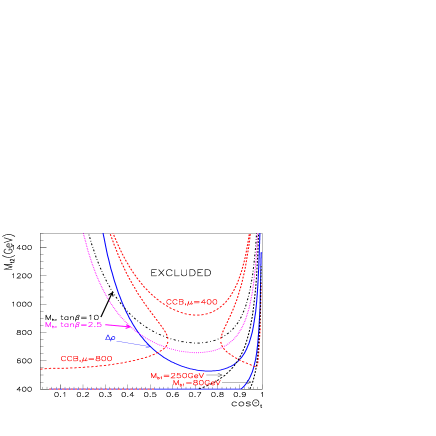
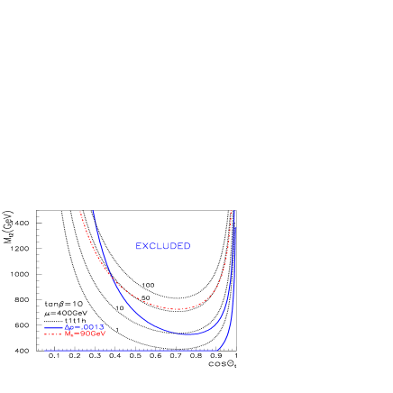
Figure 1: (a) Constraint from $\Delta\rho\leq 0.0013$ (full line), $M_{h}\geq 90$ GeV (dash-dot), CCB (dash) and $m_{\tilde{b}_{1}}$ (dash) for $\tan\beta=10$, $\mu=400$ GeV, $m_{\tilde{t}_{1}}=120$ GeV and $M_{A}=1$ TeV; the $M_{h}$ constraint for $\tan\beta=2.5$ is also shown (dot). (b) Equipotential lines (dotted) for the normalized coupling $R_{\tilde{t}_{1}}=1,10,50,100$ with $\tan\beta=10$ and $\mu=400$ GeV. The exclusion regions corresponding to $\Delta\rho\leq.0013$ and $M_{h}\leq 90$ GeV are also reproduced.

Fig. 1 shows how the parameter space is restricted by the previous constraints and which values of the ratio $R_{\tilde{t}_{1}}$ are allowed. In Fig. 1a, the excluded region in the plane $(\cos\theta_{\tilde{t}},m_{{\tilde{t}}_{2}}$) is within the respective boundaries indicated. Note that for $\cos\theta_{\tilde{t}}\approx 1$, the $\Delta\rho$ constraint also excludes the region to the right of the second branch of the $\Delta\rho$ curve where the present limit on the mass of the sbottom is contained. Requiring $m_{\tilde{b}_{1}}\geq 250$ GeV excludes the region to the right of the curve. The CCB constraint for $\mu=800$ GeV is also displayed, the excluded region lies between the two “CCB, $\mu=800$” curves. In Fig. 1b, we show the equipotential lines for the normalized coupling $R_{\tilde{t}_{1}}$. The exclusion regions corresponding to $\Delta\rho\leq.0013$ and $M_{h}\leq 90$ GeV are also reproduced. In all cases $M_{2}=-\mu$ and a common gaugino mass at the GUT scale are assumed. Note that one has to make sure that the lightest stop is not the LSP, as has been always verified in our analysis. Considering that the CCB constraint is rather uncertain, it is also worth pointing out that the one used in our analysis hardly precludes points which are not already excluded by the $\Delta\rho$ and $m_{h}$ constraints.

3 Higgs boson signals at the LHC

In this section, we will discuss what might happen to the search for the lightest MSSM Higgs boson $h$ at the LHC, if one allows all sparticles but the stops (and to a lesser extent the charginos and neutralinos) to be rather heavy. We will first discuss the effects of stop loops in the gluon–gluon fusion mechanism, $gg\rightarrow h$, and in the main Higgs detection channel, the two–photon decay $h\rightarrow\gamma\gamma$, and then discuss the associated production of stops with the light Higgs boson $h$ and possibly $A$.

3.1 Stop loop effects

Since the $h\tilde{t}_{1}\tilde{t}_{1}$ vertex eq. (2) does not have a definite sign [for no mixing the positive $m_{t}^{2}$ component dominates while for maximal mixing the negative component $\frac{1}{4}\sin^{2}(2\theta_{\tilde{t}})(m_{\tilde{t}_{1}}^{2}-m_{\tilde{t}_{2}}^{2})$ is the leading one], the stop loop contributions can interfere either destructively or constructively with the top loop contributions in the $gg\rightarrow h$ and $h\rightarrow\gamma\gamma$ processes. Noting that while for $gg\rightarrow h$ only top/stop loops are present, for the decay $h\rightarrow\gamma\gamma$, the additional contributions from $W$ loops are dominant and have a destructive interference with the top contributions. This means that if the rate for $h\rightarrow gg$ is suppressed, there will be a slight increase in $h\rightarrow\gamma\gamma$ decay width and vice versa. Therefore either the rate for the inclusive channel $gg\rightarrow h\rightarrow\gamma\gamma$ is enhanced or the rate for the associated Higgs production $pp\to Wh,Zh,t\bar{t}h$ [17] with $h\rightarrow\gamma\gamma$ is enhanced. It is important to stress that, in any case, the rate for the associated $t\bar{t}h$ production with the subsequent decay $h\rightarrow b\bar{b}$ is hardly affected by stop loops and will always help in these scenarii, as will be discussed later.

We begin our analysis by defining the ratio $R_{\gamma\gamma}\equiv R_{h\rightarrow\gamma\gamma}$ which is the branching ratio of the lightest SUSY Higgs boson decay into two photons over that of the SM for the same Higgs mass. In the decoupling regime, $M_{A}\gg M_{Z}$, this ratio is affected only by SUSY–particle loops; in this case the ratio is also sensibly the same as the ratio for associated production of the $h$ boson with $W,Z$ bosons and/or with $t\bar{t}$ pairs, with $h$ decaying into $\gamma\gamma$. We also define $R_{gg\gamma\gamma}$ as the ratio for the signal in the direct production channel $gg\rightarrow h$ times the branching ratio for the $h\rightarrow\gamma\gamma$ decay in the two models. The $gg$ and $\gamma\gamma$ decay widths are obtained with the help of the program HDECAY [16].

Fig. 2 summarizes the contribution of stop loops to these ratios, for $\tan\beta=2.5,\mu=-M_{2}=250$ GeV and $M_{A}=1$ TeV. To maximize the effect of stop mixing, $\sin(2\theta_{\tilde{t}})\simeq 1$, we assume that $\tilde{m}_{\tilde{Q}_{3}}\simeq\tilde{m}_{\tilde{U}_{3R}}$. From this figure, one can see that:

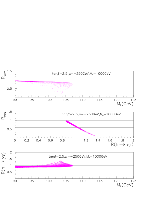
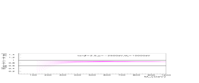
Figure 2: Higgs boson $(h)$ production and decay ratios at the LHC for $\tilde{m}_{\tilde{Q}_{3}}\simeq\tilde{m}_{\tilde{U}_{3R}}$ at $\tan\beta=2.5$ and large $M_{A}$. Figures are scanned over $\tilde{m}_{\tilde{Q}_{3}}$ and $A_{t}$ within the constraints discussed above.

– The $h\rightarrow\gamma\gamma$ branching ratio is only mildly affected [less than $\sim 30\%$] by the contributions of the stop loops which can be of either sign. This is mainly due to the fact that the $W$ contribution to the $h\gamma\gamma$ vertex is largely dominant in the decoupling limit.

– The $hgg$ coupling is always reduced compared to the SM case for large stop mixing and rather light stops can lead to a strong reduction in the rate of the inclusive production channel $gg\rightarrow h$. The suppression factor can be as low as $1/10$ whereas a benchmark for discovery is about $\sim 1/2$ [although this benchmark depends slightly on the Higgs boson mass]. The suppression occurs for rather large, though not maximal, Higgs boson masses where the efficiencies are better than for smaller Higgs masses.

– For very heavy stops which should decouple from the $hgg$ and $h\gamma\gamma$ vertices, the ratio $R_{gg\gamma\gamma}$ could be different from unity since charginos could be also light and might give small contributions to the $h\to\gamma\gamma$ decay width in the MSSM.

3.2 Associated Higgs production with stops

If the mixing in the stop sector is large, one of the top squarks can be rather light and at the same time, its couplings to the Higgs boson can be strongly enhanced. The associated production process $pp\to q\bar{q}/gg\to h\tilde{t}_{1}\tilde{t}_{1}$ might then be favored by phase space and the cross sections might be significantly large. This process is thus worth investigating at the LHC.

In view of the implementation of the process $pp\to q\bar{q}/gg\to\tilde{t}_{1}\tilde{t}_{1}h$ into an event generator, it is useful to give a “model independent” description of the production cross section in the continuum, in terms of the parameters $m_{\tilde{t}_{1}},M_{h}$ [besides $\alpha_{s}$, $m_{t}$ etc…]. One can tabulate, in a way which can be read externally, the cross section according to selected values of $M_{h},m_{\tilde{t}_{1}}$ together with the coupling $V_{\tilde{t}_{1}\tilde{t}_{1}h}$ [for simplicity and as a first step, one can take the vertex $V_{\tilde{t}_{1}\tilde{t}_{1}h}$ such that $R_{\tilde{t}_{1}}=1$, i.e. in the large $M_{A}$ limit, no $\tilde{t}$ mixing and $D$–terms].

The generator of partonic events for $pp\to\tilde{t}_{1}\tilde{t}_{1}h$ can be created by using the package CompHEP [18] and may be down-loaded at this http address [19]. The events can be used as an external process input in PYTHIA [20] or ISAJET for further decay and hadronization to simulate full events at the level of detectable particles. The $\tilde{t}_{1}\tilde{t}_{1}h$ coupling is evaluated as a user’s function thus allowing for an interface with any SUSY model. The generator also includes, as an option, the event generation of the SM process $pp\to q\bar{q}/gg\to t\bar{t}$+Higgs.

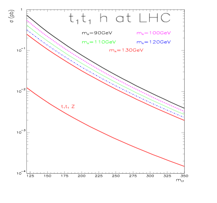
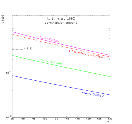
Figure 3: The cross section $pp\to\tilde{t}_{1}\tilde{t}_{1}h$ (and similar processes) at the LHC as functions of $m_{\tilde{t}_{1}}$ (left) and $M_{h}$ (right) for a range of $M_{h}$ and $m_{\tilde{t}_{1}}$ values. See text for details.

As an illustration, defined reference cross sections calculated with the help of CompHEP are displayed in Fig. 3. The cross sections are shown as functions of $M_{h}(m_{\tilde{t}_{1}})$ for given values of $m_{\tilde{t}_{1}}(M_{h})$, for a $\tilde{t}_{1}\tilde{t}_{1}h$ vertex in the limit of large $M_{A}$, no mixing and no D–terms, as discussed above. Also shown are the cross sections for the processes $pp\to t\bar{t}h,t\bar{t}Z$ [where only the dominating contributions of the $gg$ initiated subprocesses are included] and $\tilde{t}_{1}\tilde{t}_{1}Z$ [where the vertex has been computed with $\cos^{2}\theta_{\tilde{t}}=1/2$, i.e. maximal mixing, and has to be rescaled by a factor $(\cos^{2}\theta_{\tilde{t}}/2-2/3s_{W}^{2})$ for other mixing values,]. We have used the CTEQ4 structure functions [22] with a scale set at the invariant mass of the subprocess.

As can be seen, the $pp\to\tilde{t}_{1}\tilde{t}_{1}h$ cross section can be large for small values of the stop and the Higgs masses, but drops precipitously with $m_{\tilde{t}_{1}}$ and to a lesser extent with $M_{h}$. The cross section is more than order of magnitude larger than $\sigma(pp\to\tilde{t}_{1}\tilde{t}_{1}Z)$ and can exceed the one for the SM–like process $pp\to t\bar{t}h$ for strong enough mixing $R_{\tilde{t}}\gg 1$ and light $\tilde{t}_{1}$.

Figure 4: The $pp\to\tilde{t}_{1}\tilde{t}_{1}h$ cross sections at the LHC as a function of $m_{\tilde{t}_{1}}$ (left) and a scan on $m_{\tilde{Q}}$ and $A_{t}$ (right). Shown also are points that pass $\sigma_{\tilde{t}_{1}\tilde{t}_{1}h}>300$ fb and $m_{\tilde{t}_{1}}\geq 150$ GeV, imposing $\Delta\rho\leq.0013$ (top) or $\Delta\rho\leq.0026$ (bottom).

If one takes the value $\sigma(\tilde{t}_{1}\tilde{t}_{1}h)>300$ fb as a benchmark cross section value for observing this process at the LHC, and using the constraint on the maximum values of the $\tilde{t}_{1}\tilde{t}_{1}h$ coupling, values of $m_{\tilde{t}_{1}}\geq 250$ GeV are hardly accessible at the LHC. This is shown in Fig. 4 where the $pp\to\tilde{t}_{1}\tilde{t}_{1}h$ cross section is shown as a function of $m_{\tilde{t}_{1}}$ taking all soft squark masses equal for $\tan\beta=2.5$ and imposing $\Delta\rho\leq.0013$. A scan on the common soft breaking scalar mass and $A_{t}$ has also been performed; shown are points that pass the criteria $\sigma_{\tilde{t}_{1}\tilde{t}_{1}h}>300$ fb and for which $m_{\tilde{t}_{1}}\geq 150$ GeV. Larger values of the stop mass can be reached if ones allows a $2\sigma$ variation on the $\Delta\rho$ constraint, as shown in the figures at the bottom.

3.3 Comparison of inclusive and associated production processes

Let us now make a global discussion on the stop effects in both type of processes for Higgs boson production, $gg\rightarrow h\to\gamma\gamma$ and $pp\to\tilde{t}_{1}\tilde{t}_{1}h$. The two cross sections are shown in Fig. 5 in the decoupling limit for $\tan\beta=2.5$ and equal soft breaking scalar masses. As can be seen, the suppression of the rate in the inclusive production channel is compensated by a rate increase in the associated production channel. When the suppression factor in the inclusive production is below $0.5$ making discovery in this channel difficult, the cross section for the process $\tilde{t}_{1}\tilde{t}_{1}h$ is above $200$ fb. As discussed previously, a benchmark value for the cross section allowing the discovery of the Higgs boson in the $pp\to\tilde{t}_{1}\tilde{t}_{1}h$ channel has been estimated to $\sigma\sim 300$ fb. Therefore for some values of the parameters, neither the inclusive nor the $pp\to\tilde{t}_{1}\tilde{t}_{1}h$ channels can be accessed. However, one also sees that for these same points one can without difficulty use the usual $pp\to Wh/Zh,t\bar{t}h$ search modes.

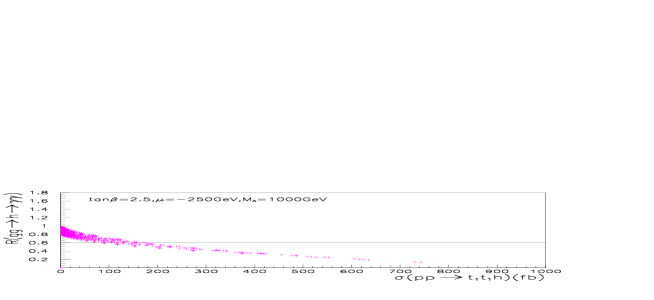
Figure 5: The cross sections for the inclusive and associated Higgs production at the LHC for $\tilde{m}_{\tilde{Q}_{3}}\simeq\tilde{m}_{\tilde{U}_{3R}}$ at $\tan\beta=2.5$ and large $M_{A}$. Figures are scanned over $\tilde{m}_{\tilde{Q}_{3}}$ and $A_{t}$.

Therefore with the remark that the process $pp\to t\bar{t}h$ [with $h\rightarrow b\bar{b}$] should allow for Higgs boson discovery at the LHC within this scenario, one should salvage the detection the $h$ boson with the bonus that the stop should also be observed. Even though one may have to wait for the higher luminosity stage, the scenario with light stops and large couplings offer much better prospects than previously thought.

The assumption of an equal value for the soft scalar masses at the weak scale is rather unnatural [see later in mSUGRA] and could be relaxed. To illustrate the fact that large suppression factors in the inclusive production channel, though not as dramatic as in the previous case, still occur we show in Fig. 6 typical $R$ ratios for unequal values of the soft masses. What is most interesting is that, as soon as $\sin(2\theta_{\tilde{t}})\neq 1$, the non–diagonal decay channel $\tilde{t}_{2}\rightarrow\tilde{t}_{1}h$ opens up and can have an appreciable branching ratio. This can be seen by inspection of the $V_{\tilde{t}_{1}\tilde{t}_{2}h}$ coupling, for which the leading component is proportional to: $V_{\tilde{t}_{1}\tilde{t}_{2}h}\propto g/(4M_{W})\sin 4\theta_{\tilde{t}}\,(m_{\tilde{t}_{1}}^{2}-m_{\tilde{t}_{2}}^{2})$. Considering that if the $\tilde{t}_{2}$ mass is not excessively large, $\tilde{t}_{2}$ is produced in abundance and this cascade decay can provide more Higgs bosons than through the continuum $pp\to\tilde{t}_{1}\tilde{t}_{1}h$ production.

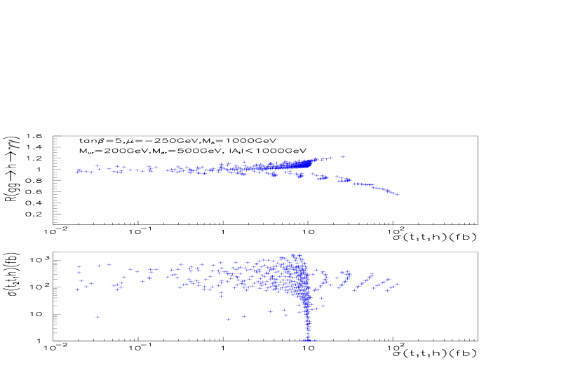
Figure 6: Higgs boson production rates at the LHC for unequal soft breaking scalar masses in the decoupling limit $M_{A}=$1TeV and $\sigma(pp\to\tilde{t}_{2}\tilde{t}_{1}h)$ vs $\sigma(pp\to\tilde{t}_{1}\tilde{t}_{1}h)$.

Perhaps even more interesting, is the case when $M_{A}$ is not too large. For large values of $A_{t}$, and even when $\sin 2\theta_{\tilde{t}}\simeq 1$, one can have a large decay rate $\tilde{t}_{2}\rightarrow\tilde{t}_{1}A$ since the $A\tilde{t}_{1}\tilde{t}_{2}$ coupling can be large $V_{\tilde{t}_{1}\tilde{t}_{2}A}\propto gm_{t}/(2M_{W})(A_{t}/\tan\beta-\mu)$, as shown in Fig. 7. This coupling is generally larger than the $\tilde{t}_{2}\tilde{t}_{1}H$ coupling and hence, within these scenarii, the decay $\tilde{t}_{2}\to\tilde{t}_{1}A$ is most likely to occur than the decay into the heavier $H$ boson, $\tilde{t}_{2}\to H\tilde{t}_{1}$.

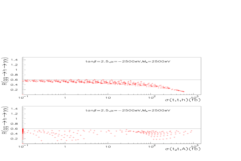
Figure 7: Higgs boson production and decay rates at the LHC for low values of $M_{A}$.

Finally, let us make a few comments on the case of the minimal Supergravity model [23], where the only input parameters are the universal scalar mass $m_{0}$, the universal gaugino mass parameter $m_{1/2}$, the trilinear coupling $A_{0}$, $\tan\beta$ and the sign of the $\mu$ parameter. The parameters $m_{0},m_{1/2}$ and $A_{0}$ are chosen at the GUT scale and their evolution down to the weak scale is given by the RGE’s [24]. Proper breaking of the electroweak symmetry is also assumed, which fixes the parameter $|\mu|$. In what follows, the RGE’s and the proper EW symmetry breaking are solved using the program SUSPECT [25].

In the mSUGRA case the cross section can be as large as in the case of the unconstrained MSSM, but in a relatively smaller area of the SUSY parameter space. This is essentially due to the fact that it is generically very difficult to have almost degenerate $\tilde{t}_{L}$ and $\tilde{t}_{R}$ in mSUGRA, so that the stop mixing angle which is controlled by the ratio $\tilde{A}_{t}/(\tilde{m}^{2}_{\tilde{t}_{L}}-\tilde{m}^{2}_{\tilde{t}_{R}})$ can become large only for very large $\tilde{A}_{t}$. Moreover in the RG evolution [24] $|A_{t}|$ tends to decrease when the energy scale is decreasing from GUT to low-energy. This makes a large $A_{t}$ value at low energy less likely, since $A_{0}=A_{t}({\rm GUT})$ would have to be even larger, which may conflict with e.g. the CCB constraints. The only way to have an increasing $|A_{t}|$ when running down to low energy is if $A_{0}<0$ with $A_{0}$ small enough. This requires a large $m_{1/2}$ value, which implies not too small $m_{\tilde{t}_{1}}$.

Thus the mixing in the stop sector is, in general, not as large as in the unconstrained MSSM and the $\tilde{t}_{1}\tilde{t}_{1}h$ coupling for instance is, in general, smaller than in the previous case. This implies that the rate for the inclusive production and detection channel $gg\rightarrow h\rightarrow\gamma\gamma$ [in the decoupling limit] is not as dramatically different from the rate in the SM, as it can be in the unconstrained MSSM. Furthermore, the milder mixing results in a smaller cross sections for the process $pp\to\tilde{t}_{1}\tilde{t}_{1}h$ as is shown in Fig. 8 for LHC energies. However, for large $\tan\beta$ values, the pseudoscalar $A$ boson tends to be rather light in mSUGRA, opening the possibility for the decay $\tilde{t}_{2}\to\tilde{t}_{1}A$ to occur with an appreciable rate as shown in Fig. 8b.

Note that one should also easily observe the pseudoscalar $A$ boson in the loop mediated process $gg\to A$ since the rate is strongly enhanced for large $\tan\beta$ and, because of CP–invariance, light stop [or sbottom] loops cannot contribute to the process.

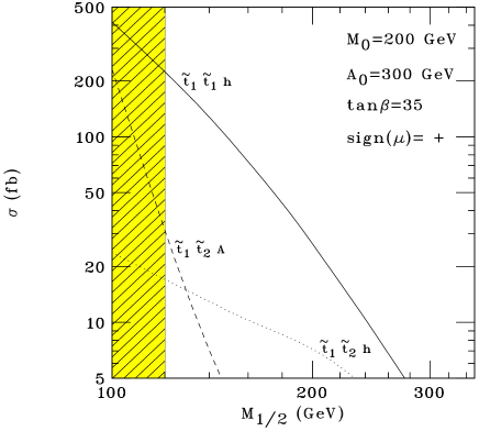
Figure 8: Cross sections in mSUGRA at LHC: a) $\sigma(pp\to\tilde{t}_{1}\tilde{t}_{1}h)$ for $m_{1/2}=0.3$ TeV, $A_{0}=2$ TeV, $\tan\beta=2.5,30$. b) $\sigma(pp\to\tilde{t}_{1}\tilde{t}_{1}h,\tilde{t}_{1}\tilde{t}_{2}h,\tilde{t}_{1}\tilde{t}_{2}A)$ for $m_{0}=0.2$ TeV, $A_{0}=0.3$ TeV and $\tan\beta=35$. For the spectrum, SUSPECT is used in a) and ISAJET in b).

1 Introduction

Considerable attention has been devoted to double Higgs boson production at future $e^{+}e^{-}$ and hadron colliders, both in the Standard Model (SM) and the MSSM [1, 2, 3]. For the SM, detailed signal-to-background studies already exist for a LC environment [3], for both ‘reducible’ and ‘irreducible’ backgrounds [4, 5], which have assessed the feasibility of experimental analyses. At the LHC, since here the typical SM signal cross sections are of the order of 10 fb [2], high integrated luminosities would be needed to generate a statistically large enough sample of double Higgs events. These would be further obscured by an overwhelming background, making their selection and analysis in a hadronic environment extremely difficult. Thus, in this contribution we will concentrate only on the case of the MSSM.

In the Supersymmetric (SUSY) scenario, the phenomenological potential of these reactions is two-fold. Firstly, in some specific cases, they can furnish new discovery channels for Higgs bosons. Secondly, they are all dependent upon several triple Higgs self-couplings of the theory, which can then be tested by comparing theoretical predictions with experimental measurements. This is the first step in the reconstruction of the Higgs potential itself.

The Higgs Working Group (WG) has focused much of its attention in assessing the viability of these reactions at future TeV colliders. However, the number of such processes is very large both at the LHC and a LC [2, 3], so only a few ‘reference’ reactions could be studied in the context of this Workshop. Work is in progress for the longer term, which aims to cover most of the double Higgs production and decay phenomenology at both accelerators [6].

These reference reactions were chosen to be the gluon–fusion mechanism, $gg\to hh$, for the LHC (see top of Fig. 1) and the Higgs–strahlung process, $e^{+}e^{-}\to hhZ$, for the LC (see bottom of Fig. 1), where $h$ is the lightest of the MSSM scalar Higgs bosons. The reason for this preference is simple. Firstly, a stable upper limit exists on the value of $m_{h}$, of the order of 130 GeV, now at two-loop level [7], so that its detection is potentially well within the reach of both the LHC and a LC. In contrast, the mass of all other Higgs bosons of the MSSM may vary from the electroweak (EW) scale, ${\cal O}(m_{Z})$, up to the TeV region. In addition, as noted in Ref. [2], the multi-$b$ final state in $gg\to hh\to b\bar{b}b\bar{b}$, with two resonances and large transverse momenta, may be exploited in the search for the $h$ scalar in the large $\tan\beta$ and moderate $m_{A}$ region. This is a corner of the MSSM parameter space that has so far eluded the scope of the standard Higgs production and decay modes [8]. (The symbol $A$ here denotes the pseudoscalar Higgs boson of the MSSM, and we reserve the notation $H$ for the heaviest scalar Higgs state of the model.) However, this paper will not investigate the LHC discovery potential in this mode, given the very sophisticated treatment of the background (well beyond the scope of this note) required by the assumption that no $h$ scalar state has been previously discovered (see below). This will be done in Ref. [6]. Furthermore, the $gg\to hh$ and $e^{+}e^{-}\to hhZ$ modes largely dominate double Higgs production [2, 3], at least for centre-of-mass (CM) energies of 14 TeV at the LHC and 500 GeV in the case of a LC, the default values of our analysis. (Notice that we assume no polarization of the incoming beams in $e^{+}e^{-}$ scattering.) Finally, when $m_{H}\lower 3.01385pt\hbox{$\;\stackrel{{\scriptstyle\textstyle>}}{{\sim}}\;$}2m_{h}$, the two reactions are resonant, as they can both proceed via intermediate states involving $H$ scalars, through $gg\to H$ and $e^{+}e^{-}\to HZ$, which in turn decay via $H\to hh$ [9]. Thus, the production cross sections are largely enhanced [2, 3] (up to two orders of magnitude above typical SM rates at the LHC [2]) and become clearly visible. This allows the possibility of probing the trilinear $Hhh$ vertex at one or both these colliders.

The dominant decay rate of the MSSM $h$ scalar is into $b\bar{b}$ pairs, regardless of the value of $\tan\beta$ [9]. Therefore, the final signatures of our reference reactions always involve four $b$-quarks in the final state. (In the case of a LC environment, a further trigger on the accompanying $Z$ boson can be exploited.)

If one assumes very efficient tagging and high-purity sampling of $b$-quarks, the background to $hh$ events at the LHC is dominated by the irreducible QCD modes [10]. Among these, we focus here on the cases $q\bar{q},gg\to b\bar{b}b\bar{b}$, as representative of ideal $b$-tagging performances. These modes consist of a purely QCD contribution of ${\cal O}(\alpha_{s}^{4})$, an entirely EW process of ${\cal O}(\alpha_{em}^{4})$ (with no double Higgs intermediate states) and an ${\cal O}(\alpha_{s}^{2}\alpha_{em}^{2})$ component consisting of EW and QCD interactions. (Note that in the EW case only $q\bar{q}$ initiated subprocesses are allowed at tree-level.) For a LC, the final state of the signal is $b\bar{b}b\bar{b}Z$, with the $Z$ reconstructed from its decay products in some channel. Here, the EW background is of ${\cal O}(\alpha_{em}^{5})$ away from resonances (and, again, contains no more than one intermediate Higgs boson), whereas the EW/QCD background is proportional to $(\alpha_{s}^{2}\alpha_{em}^{3})$.

In general, EW backgrounds can be problematic due to the presence of $Z$ vectors and single Higgs scalars yielding $b\bar{b}$ pairs, with the partons being typically at large transverse momenta and well separated. In contrast, the QCD backgrounds involve no heavy objects decaying to $b\bar{b}$ pairs and are dominated by the typical infrared (i.e., soft and collinear) QCD behavior of the partons in the final state. However, they can yield large production rates because of the strong couplings.

$gg$ to double Higgs fusion at the LHC: $gg\to hh$

double Higgs-strahlung at a LC: $e^{+}e^{-}\to hhZ$

Figure 1: Diagrams contributing to $gg\to hh$ (top) and $e^{+}e^{-}\to hhZ$ (bottom) in the MSSM.

In this study, we investigate the interplay between the signal and background at both colliders, adopting detector as well as dedicated selection cuts. We carry out our analysis at both parton and hadron level. The plan of this note is as follows. The next Section details the procedure adopted in the numerical computation. Sect. 3 displays our results and contains our discussion. Finally, in the last section, we summarize our findings and consider possible future studies.

2 Calculation

For the parton level simulation, the double Higgs production process at the LHC, via $gg$ fusion, has been simulated using the program of Ref. [11] to generate the interaction $gg\to hh$, with the matrix elements (MEs) taken at leading-order (LO) for consistency with our treatment of the background. We then perform the two $h\to b\bar{b}$ decays to obtain the actual $4b$-final state. For double Higgs production at a LC, we use a source code for the signal derived from that already used in Ref. [5]. At both colliders, amplitudes for background events were generated by means of MadGraph [12] and the HELAS package [13]. Note that interferences between signal and backgrounds, and between the various background contributions themselves, have been neglected. This is a good approximation for the interferences involving the signal because of the very narrow width of the MSSM lightest Higgs boson. Similarly, the various background subprocesses have very different topologies, and one would expect their interferences to be small in general.

The Higgs boson masses and couplings of the MSSM can be expressed at tree-level in terms of the mass of the pseudoscalar Higgs state, $m_{A}$, and the ratio of the vacuum expectation values of the two neutral fields in the two iso-doublets, $\tan\beta$. At higher order however, top and stop loop-effects can become significant. Radiative corrections in the one-loop leading $m_{t}^{4}$ approximation are parameterized by

$$\epsilon\approx\frac{3G_{F}m_{t}^{4}}{\sqrt{2}\pi^{2}\sin^{2}\beta}\log\frac{m_{S}^{2}}{m_{t}^{2}}$$ (1)

where the SUSY breaking scale is given by the common squark mass, $m_{S}$, set equal to $1$ TeV in the numerical analysis. If stop mixing effects are modest at the SUSY scale, they can be accounted for by shifting $m_{S}^{2}$ in $\epsilon$ by the amount $\Delta m_{S}^{2}=\hat{A}^{2}[1-\hat{A}^{2}/(12m_{S}^{2})]$ ($\hat{A}$ is the trilinear common coupling). The charged and neutral CP-even Higgs boson masses, and the Higgs mixing angle $\alpha$ are given in this approximation by the relations:

$$m_{H^{\pm}}^{2}\!\! = \!\!m_{A}^{2}+m_{Z}^{2}\cos^{2}\theta_{W},$$

$$m_{h,H}^{2}\!\! = \!\!\textstyle{\frac{1}{2}}[m_{A}^{2}+m_{Z}^{2}+\epsilon$$

$$\mp \sqrt{(m_{A}^{2}+m_{Z}^{2}+\epsilon)^{2}-4m_{A}^{2}m_{Z}^{2}\cos^{2}2\beta-4\epsilon(m_{A}^{2}\sin^{2}\beta+m_{Z}^{2}\cos^{2}\beta)}],$$

$$\tan 2\alpha\!\! = \!\!\tan 2\beta\frac{m_{A}^{2}+m_{Z}^{2}}{m_{A}^{2}-m_{Z}^{2}+\epsilon/\cos 2\beta}\qquad\mbox{with}\qquad-\frac{\pi}{2}\leq\alpha\leq 0,$$ (2)

as a function of $m_{A}$ and $\tan\beta$. The triple Higgs self-couplings of the MSSM can be parameterized [14, 15] in units of $M_{Z}^{2}/v$, $v=246$ GeV, as,

$$\lambda_{hhh} = 3\cos 2\alpha\sin(\beta+\alpha)+3\frac{\epsilon}{m_{Z}^{2}}\frac{\cos\alpha}{\sin\beta}\cos^{2}\alpha,$$

$$\lambda_{Hhh} = 2\sin 2\alpha\sin(\beta+\alpha)-\cos 2\alpha\cos(\beta+\alpha)+3\frac{\epsilon}{m_{Z}^{2}}\frac{\sin\alpha}{\sin\beta}\cos^{2}\alpha,$$

$$\lambda_{HHh} = -2\sin 2\alpha\cos(\beta+\alpha)-\cos 2\alpha\sin(\beta+\alpha)+3\frac{\epsilon}{m_{Z}^{2}}\frac{\cos\alpha}{\sin\beta}\sin^{2}\alpha,$$

$$\lambda_{HHH} = 3\cos 2\alpha\cos(\beta+\alpha)+3\frac{\epsilon}{m_{Z}^{2}}\frac{\sin\alpha}{\sin\beta}\sin^{2}\alpha,$$

$$\lambda_{hAA} = \cos 2\beta\sin(\beta+\alpha)+\frac{\epsilon}{m_{Z}^{2}}\frac{\cos\alpha}{\sin\beta}\cos^{2}\beta,$$

$$\lambda_{HAA} = -\cos 2\beta\cos(\beta+\alpha)+\frac{\epsilon}{m_{Z}^{2}}\frac{\sin\alpha}{\sin\beta}\cos^{2}\beta.$$ (3)

Next-to-leading order (NLO) effects are certainly dominant, though the next-to-next-to-leading order (NNLO) ones cannot entirely be neglected (especially in the Higgs mass relations). Thus, in the numerical analysis, the complete one-loop and the leading two-loop corrections to the MSSM Higgs masses and the triple Higgs self-couplings are included. The Higgs masses, widths and self-couplings have been computed using the HDECAY program described in Ref. [16], which uses a running $b$-mass in evaluating the $h\rightarrow b\bar{b}$ decay fraction. Thus, for consistency, we have evolved the value of $m_{b}$ entering the $hbb$ Yukawa couplings of the $h\rightarrow b\bar{b}$ decay currents of our processes in the same way.

For our analysis, we have considered $\tan\beta=3$ and $50$. For the LHC, high values of $\tan\beta$ produce a signal cross section much larger than the $\tan\beta=3$ scenario, over almost the entire range of $m_{A}$. However, this enhancement is due to the increase of the down-type quark-Higgs coupling, which is proportional to $\tan\beta$ itself, and serves only to magnify the dominance of the quark box diagrams of Fig. 1. Unfortunately, these graphs have no dependence on either of the two triple Higgs self-couplings entering the gluon-gluon process considered here, i.e., $\lambda_{hhh}$ and $\lambda_{Hhh}$. Thus, although the cross section is comfortably observable, all sensitivity to such vertices is lost. Therefore, the measurement of the triple Higgs self-coupling, $\lambda_{Hhh}$, is only feasible at the LHC for low $\tan\beta$ due to the resonant production of the heavy Higgs boson (see Fig. 5a of Ref. [2]).

In contrast, the cross section for double Higgs production at the LC is small for large $\tan\beta$ because there is no heavy Higgs resonance (see Fig. 8 of Ref. [3]). As soon as it becomes kinematically possible to decay the heavy Higgs into a light Higgs pair, the $ZZH$ coupling is already too small to generate a sizable cross section. Furthermore, the continuum MSSM cross section is suppressed with respect to the SM cross section since the MSSM couplings $ZZH$ and $ZZh$ vary with $\cos(\beta-\alpha)$ and $\sin(\beta-\alpha)$, respectively, with respect to the corresponding SM coupling. Notice that in this regime, at a LC, the $\lambda_{hhh}$ vertex could in principle be accessible instead, since $\lambda_{hhh}\gg\lambda_{Hhh}$ (see Fig. 2 of Ref. [3]) and because of the kinematic enhancement induced by $m_{h}\ll m_{H}$. Unfortunately, we will see that the size of the $e^{+}e^{-}\to hhZ$ cross section itself is prohibitively small.

We assume that $b$-jets are distinguishable from light-quark and gluon jets and no efficiency to tag the four $b$-quarks is included in our parton level results. We further neglect considering the possibility of the $b$-jet charge determination. Also, to simplify the calculations, the $Z$ boson appearing in the final state of the LC process is treated as on-shell and no branching ratio (BR) is applied to quantify its possible decays. In practice, one may assume that it decays leptonically (i.e., $Z\to\ell^{+}\ell^{-}$, with $\ell=e,\mu,\tau$) or hadronically into light-quark jets (i.e., $Z\to q\bar{q}$, with $q\neq b$), in order to avoid problems with $6b$-quark combinatorics. Furthermore, in the LC analysis, we have not simulated the effects of Initial State Radiation (ISR), beamstrahlung or Linac energy spread. Indeed, we expect them to affect signal and backgrounds rather similarly, so we can neglect them for the time being. Indeed, since a detailed phenomenological study, including both hadronization and detector effects, already exists for the case of double Higgs-strahlung in $e^{+}e^{-}$ [4], whose conclusions basically support those attained in the theoretical study of Ref. [5], we limit ourselves here to update the latter to the case of the MSSM.

So far only resonant production $gg$ $\to$ $H$ $\to$ $hh$ $\to$ $b\bar{b}b\bar{b}$ has been investigated [10], with full hadronic and detector simulation and considering also the (large) QCD backgrounds, and a similar study does not exist for continuum double Higgs production at the LHC. (See Ref. [17] for a detailed account of the $gg\to H$ $\to$ $hh$ $\to$ $\gamma\gamma b\bar{b}$ decay channel.) The event simulation has been performed by using a special version of PYTHIA [18], in which the relevant LO MEs for double Higgs production of Ref. [11] have been implemented by M. El Kacimi and R. Lafaye. These MEs take into account both continuum and resonant double Higgs boson production and their interferences. (The insertion of those for $e^{+}e^{-}$ processes is in progress.) The PYTHIA interface to HDECAY has been exploited in order to generate the MSSM Higgs mass spectrum and the relevant Higgs BRs, thus maintaining consistency with the parton level approach. As for the LHC detector simulation, the fast simulation package was used, with high luminosity (i.e., $\int{\cal L}dt=100$ fb^-1) parameters.

The motivation for our study is twofold. On the one hand, to complement the studies of Ref. [10] by also considering the continuum production $gg\to hh\to b\bar{b}b\bar{b}$ at large $\tan\beta$. On the other hand, to explore the possibility of further kinematic suppression of the various irreducible backgrounds to the resonant channel at small $\tan\beta$.

3 Results

3.1 The LHC analysis

In our LHC analysis, following the discussion in Sect. 2, we focus most of our attention on the case $\tan\beta=3$, with $m_{A}=210$ GeV, although other combinations of these two MSSM parameters will also be considered. We further set $A=-\mu=1$ TeV and take all sparticle masses (and other SUSY scales) to be as large as $1$ TeV.

3.1.1 $gg\to hh\to b\bar{b}b\bar{b}$ at parton level

In our parton level analysis, we identify jets with the partons from which they originate (without smearing the momenta) and apply all cuts directly to the partons. We mimic the finite coverage of the LHC detectors by imposing a transverse momentum threshold on each of the four $b$-jets,

$$p_{T}({b})>30~{}{\mathrm{GeV}}$$ (4)

and requiring their pseudorapidity to be

$$|\eta({b})|<2.5.$$ (5)

Also, to allow for their detection as separate objects, we impose an isolation criterium among $b$-jets,

$$\Delta R({bb})>0.4,$$ (6)

by means of the usual cone variable $\Delta R({ij})=\sqrt{\Delta\eta({ij})^{2}+\Delta\phi({ij})^{2}}$, defined in terms of relative differences in pseudo-rapidity $\eta_{ij}$ and azimuth $\phi_{ij}$ of the $i$-th and $j$-th $b$-jets.

As preliminary and very basic selection cuts (also to help the stability of the numerical integration), we have required that the invariant mass of the entire $4b$-system is at least twice the mass of the lightest MSSM Higgs boson (apart from mass resolution and gluon emission effects), e.g.,

$$m({bbbb})\geq 2m_{h}-40~{}{\rm{GeV}},$$ (7)

and that exactly two $h$-resonances are reconstructed, such that

$$|m({bb})-m_{h}|<20~{}{\mathrm{GeV}}.$$ (8)

In doing so, we implicitly assume that the $h$ scalar boson has already been discovered and its mass measured through some other channel, as we have already intimated in the Introduction.

Figure 2: Distributions in transverse momentum of the four $p_{T}$-ordered $b$-jets in $gg\to hh\to b\bar{b}b\bar{b}$ and in the QCD background, after the cuts (4)–(8) at the LHC, for $\tan\beta=3$, $m_{h}=104$ GeV and $m_{H}\simeq 220$ GeV. Normalization is to unity.

After the above cuts have been implemented, we have found that the two $4b$-backgrounds proceeding through EW interactions are negligible compared to the pure QCD process. In fact, the constraints described in eqs. (7)–(8) produce the strongest suppression, almost completely washing out the relatively enhancing effects that the cuts in (4)–(6) have on the EW components of the backgrounds with respect to the pure QCD one, owning to the intermediate production of massive $Z$ bosons in the former. In the end, the production rates of the three subprocesses scale approximately as their coupling strengths: i.e., ${\cal O}(\alpha_{s}^{4})$ : ${\cal O}(\alpha_{s}^{2}\alpha_{em}^{2})$ : ${\cal O}(\alpha_{em}^{4})$. Therefore, in the reminder of our analysis, we will neglect EW effects, as they represent not more than a 10% correction to the QCD rates, which are in turn affected by much larger QCD $K$-factors. As for the pure QCD background itself, it hugely overwhelms the double Higgs signal at this stage. The cross section of the former is about 7.85 pb, whereas that of the latter is approximately 0.16 pb.

To appreciate the dominance of the $m_{h}$ cuts, one may refer to Fig. 2, where the distributions in transverse momentum of the four $p_{T}$-ordered $b$-quarks (such that $p_{T}(b_{1})>...>p_{T}(b_{4})$) of both signal and QCD background are shown. Having asked the four $b$-jets of the background to closely emulate the $gg\to hh\to b\bar{b}b\bar{b}$ kinematics, it is not surprising to see a ‘degeneracy’ in the shape of all spectra. Clearly, no further background suppression can be gained by increasing the $p_{T}(b)$ cuts. The same can be said for $\eta({b})$ and $\Delta R({bb})$. Others quantities ought to be exploited.

Figure 3: Distributions in minimum relative angle (in radians) in the $4b$-system rest frame between two $b$-jets reconstructing $m_{h}$ in $gg\to hh\to b\bar{b}b\bar{b}$ and in the QCD background, after the cuts (4)–(8) at the LHC, for $\tan\beta=3$, $m_{h}=104$ GeV and $m_{H}\simeq 220$ GeV. Normalization is to unity.

In Fig. 3, we present the signal and QCD background distributions in the minimum angle formed between the two $b$-quarks coming from the ‘same Higgs’ (i.e., those fulfilling the cuts in (8)) in the $4b$-system rest frame (the plot is rater similar for the maximum angle, thus also on average). There, one can see a strong tendency of the two $2b$-pairs produced in the Higgs decays to lie back-to-back, reflecting the $2\to 2$ intermediate dynamics of Higgs pair production via $gg\to hh$. Missing such kinematically constrained virtual state, the QCD background shows a much larger angular spread towards small $\theta_{\rm{min}}(bb)$ values, eventually tamed by the isolation cut (6).

The somewhat peculiar shape of the signal distribution is due to destructive interference. Recall that the signal contains not only diagrams proceeding via a heavy Higgs resonance (the upper-left hand graph of Fig. 1), which results in the large peak in Fig. 3, but also contains a continuum contribution mediated by box graphs (the upper-right hand graph of Fig. 1). These two contributions destructively interfere leading to the depletion of events between the large back-to-back peak and the small remaining ’bump’ of the continuum contribution as seen in Fig. 3.

In the end, a good criterium to enhance the signal-to-background ratio ($S/B$) is to require, e.g., $\theta({bb})>2.4$ radians, i.e., a separation between the $2b$-jets reconstructing the lightest Higgs boson mass of about 140 degrees in angle. (Incidentally, we also have investigated the angle that each of these $2b$-pairs form with the beam axis, but found no significant difference between signal and QCD background).

Figure 4: Distributions in thrust in the rest frame of the $4b$-system in $gg\to hh\to b\bar{b}b\bar{b}$ and in the QCD background, after the cuts (4)–(8) at the LHC, for $\tan\beta=3$, $m_{h}=104$ GeV and $m_{H}\simeq 220$ GeV. Normalization is to unity.

An additional consequence that one should expect from the presence of two intermediate massive objects in $gg\to hh\to b\bar{b}b\bar{b}$ events is the spherical appearance of the jets in the final state, in contrast to the usual planar behavior of the infrared QCD interactions. These phenomena can be appreciated in Fig. 4. Notice there the strong tendency of the background to yield high thrust configurations, again controlled by the separation cuts when $T$ approaches unity. On the contrary, the average value of the thrust in the signal is much lower, being the effect of accidental pairings of ‘wrong’ $2b$-pairs (the shoulder at high thrust values) marginal. An effective selection cut seems to be, e.g., $T<0.85$.

Figure 5: Distributions in invariant mass of the $4b$-system in $gg\to hh\to b\bar{b}b\bar{b}$ and in the QCD background, after the cuts (4)–(8) at the LHC, for $\tan\beta=3$, $m_{h}=104$ GeV and $m_{H}\simeq 220$ GeV. Normalization is to unity. The left hand plot shows both the signal (solid curve) and the QCD background (dashed curve), distributed in 5 GeV bins. The same signal is also shown as a histogram for a more experimentally realistic binning of 13 GeV. The right hand plot also shows the signal (collected in 5 GeV wide bins) on a logarithmic scale. Here the structure of the continuum contribution (and its destructive interference with the heavy Higgs decay contribution) can be seen.

Furthermore, if the heavy Higgs mass is sufficiently well measured at the LHC then one can exploit the large fraction [2] of $4b$-events which peak at $m_{H}$ in the signal, as dictated by the $H\to hh$ decay, improving the signal-to-background ratio. This peak at $m_{H}$ can be clearly seen in the left hand plot of Fig. 5, where it dominates the QCD background, even for bins 13 GeV wide. In fact, not only could the QCD background be considerably suppressed but also those contributions to $gg\to hh$ not proceeding through an intermediate $H$ state should be removed, this greatly enhancing the sensitivity of the signal process to the $\lambda_{Hhh}$ coupling. This can be seen in the right hand plot of Fig. 5 where the signal is shown on a logarithmic scale. The continuum contribution due to the box graphs (and its destructive interference with the heavy Higgs decay contribution) is now evident although one should note that it is considerably suppressed compared to the peak at $m_{H}$.

Now, if a less than 10% mass resolution can be achieved on the light and heavy Higgs masses, then one can tighten cut (8) to $|m({bb})-m_{h}|<10$ GeV and introduce the additional cut $|m({bbbb})-m_{H}|<20$ GeV. These cuts taken together with those in $\theta({bb})$ and $T$ already suggested, reduce the QCD background to the same level as the signal. In fact, we have found that the cross section of the background drops to approximately 174 fb whereas that of the signal remains as large as 126 fb, this yielding a very high statistical significance at high luminosity. Even for less optimistic mass resolutions the signal-to-background ratio is still significantly large. For example, selecting events with $|m(bb)-m_{h}|<20$ GeV and $|m(bbbb)-m_{H}|<40$ GeV, the corresponding numbers are approximately 102 fb for the signal and 453 fb for the background. Notice that the signal actually decreases as these Higgs mass windows are made larger. This is due to our insistence that exactly two $b\bar{b}$ pairs should reconstruct the light Higgs mass. As the light Higgs mass window is enlarged from $m_{h}\pm 10$ GeV to $m_{h}\pm 20$ GeV, it becomes more likely that accidental pairings reconstruct the light Higgs boson. Since one is then unable to unambiguously assign the $b$ quarks to the light Higgs bosons, the event is rejected and the signal drops.

Although we have discussed here an ideal situation which is difficult to match with more sophisticated hadronic and detector simulations, it still demonstrates that the measurement of the $\lambda_{Hhh}$ coupling could be well within the potential of the LHC, at least for our particular choice of MSSM parameters. Comforted by such a conclusion, we now move on to more realistic studies.

3.1.2 $gg\to hh\to b\bar{b}b\bar{b}$ at the LHC experiments

Although the LHC experiments will be the first where one can attempt to measure the Higgs self-couplings, the analysis is very challenging because of the smallness of the production cross sections. Even in the most favorable cases, the production rate is never larger than a few picobarns, already including one-loop QCD corrections, as computed in Ref. [11]. The cross sections at this accuracy are given in Tab. 1, for the resonant process (case 1 with $m_{H}=220$ GeV) as well as three non resonant scenarios: one at the same $\tan\beta$ but with the $H\to hh$ decay channel closed (case 2), a second at very large $\tan\beta$ and no visible resonance (case 3) and, finally, the SM option (case 4, where $m_{h}$ identifies with the mass of the standard Higgs state).

case	model	$\tan\beta$	$m_{h}$ (GeV)	$A$ (TeV)	$\mu$ (TeV)	$\sigma$ (fb)	dominant mode
1	MSSM	3	104	$+1$	$-1$	2000	$gg\to H\to hh$
2	MSSM	3	100	$+1$	$-1$	20	$gg\to hh$
3	MSSM	50	105	$+1$	$+1$	5000	$gg\to hh$
4	SM	-	105	-	-	40	$gg\to hh$

Table 1: Cross sections for double Higgs production $hh$ at the LHC via gluon-gluon fusion at NLO accuracy, for three possible configurations of the MSSM and in the SM as well.

3.1.3 LHC trigger acceptance

For $4b$-final states, possible LHC triggers are high $p_{T}$ electron/muons and jets. As an example, the foreseen ATLAS level 1 trigger thresholds on $p_{T}$ and acceptance for a $4b$-selection (with the four $b$-jets reconstructed in the detector) are given in Tab. 2, assuming the LHC to be running at high luminosity.

trigger type:	1 $e$	1 $\mu$	2 $\mu$	1 jet	3 jets	4 jets	total
$p_{T}$ in GeV	30	20	10	290	130	90
case 1, $\epsilon(bbbb)$ in %	0.01	0.01	0.4	0.08	0.08	0.05	0.53
case 2	$<0.01$	$<0.01$	2.1	2.9	3.8	4.2	8.8
case 3	$<0.01$	$<0.01$	2.2	2.7	3.8	4.1	8.7
case 4	$<0.01$	$<0.01$	2.0	2.5	3.3	3.6	7.8

Table 2: Kinematical acceptance of the ATLAS detector to trigger four $b$-jets (including detector acceptance) at high luminosity.

The overall trigger acceptance is at best 8–9%, for cases 2,3,4. The very low efficiency for case 1 is clearly a consequence of the small value of the difference $m_{H}-2m_{h}$, translating into a softer $p_{T}(b)$ spectrum with respect to the other cases (compare the left-hand with the right-hand side of Fig. 6). One can further see in the left-hand plot of Fig. 6 that the bulk of the signal lies below the lowest $p_{T}(b)$ threshold of Tab. 2 (i.e., $90$ GeV), so that adopting smaller trigger thresholds could result in a dramatic enhancement of our efficiency. Of course, this would also substantially increase the low transverse momentum QCD background, as we can see in the parton level analysis of Fig. 2.

For example, by lowering the thresholds to 180, 80 and 50 GeV for 1, 3 and 4 jets, respectively (compare to Tab. 2), the overall trigger acceptance on the signal goes up to 1.8%, i.e., by almost a factor of 4. Meanwhile though, the ATLAS level-1 jet trigger rates increase by a factor of 10 [19]. Anyhow, even for our poor default value of $\epsilon(bbbb)$ in Tab. 2, we will see that case 1 still yields a reasonable number of events in the end. Optimizations of the $b$-jet transverse momentum thresholds are in progress [6].

Figure 6: Reconstructed transverse energy/momentum for $b$-jets in $gg\to hh\to b\bar{b}b\bar{b}$ events of case 1 (left plot) and $b$-jets in $gg\to hh\to b\bar{b}b\bar{b}$ events of case 2 (right plot) with ATLAS fast simulation [20] at high luminosity. Normalization is arbitrary.

3.1.4 LHC events selection for $gg\to hh\to b\bar{b}b\bar{b}$

Jets are reconstructed merging tracks inside $\Delta R(bb)=0.4$. Only jets with transverse energy/momentum greater than 30 GeV and with $|\eta(b)|<2.5$ are kept. (Thus, the same cuts as in the parton level analysis, now applied instead to jets.) The effect from pile up is included in the resolution. A jet energy correction is then applied.

Figure 7: Reconstructed invariant mass distribution of $2b$-jet pairs in continuum $gg\to hh\to b\bar{b}b\bar{b}$ events (case 2) with the fast simulation at high luminosity. Normalization is arbitrary. (Results of a Gaussian fit are also given.)

Figure 8: Reconstructed $\Delta R(bb,bb)$ between $2b$-jet systems from $h\to bb$ decays in continuum $gg\to hh\to b\bar{b}b\bar{b}$ events (case 2) with the fast simulation at high luminosity. The dashed histogram shows the same distribution for all pairs of jets. Normalization is arbitrary.

The invariant masses of each jet pair can then be computed. Assuming that the lightest Higgs boson mass is known, events with $m(bb)$ sufficiently close to $m_{h}$ can efficiently be selected, see Fig. 7. Another cut on the $\Delta R(bb,bb)$ between pairs of $b$-jets can also be applied to reduce the intrinsic combinatorial background, since the latter concentrates at large $\Delta R(bb,bb)$ values, see Fig. 8.

Figure 9: Reconstructed $4b$-jet invariant mass for $b$-jets coming from the $hh$ pair in $gg\to hh\to b\bar{b}b\bar{b}$ events (case 1) with the fast simulation at high luminosity. The dashed histogram shows the same distribution for all groups of four jets. Normalization is arbitrary. (Results of a Gaussian fit to the first spectrum are also given.)

For case 1, as already discussed, we can further impose that the invariant mass of the four $b$-jets should be the heavy Higgs mass, $m_{H}$, in order to select the $H\to hh$ resonance, as confirmed by Fig. 9. In the other three cases, where the $H\to hh$ splitting is no longer dominant (MSSM) or non-existent (SM), one can still insist that the $4b$-jet invariant mass should be higher than two times the lightest Higgs mass, see Fig. 10 and recall eq. (7). Finally, following Fig. 11, by constraining the $b$-jets pairs four-momenta around the known light Higgs mass value, $m_{h}$, one can further reject the intrinsic background by means of the $m(bbbb)$ spectrum.

Figure 10: Reconstructed $4b$-jet invariant mass for $b$-jets coming from the $hh$ pair in $gg\to hh\to b\bar{b}b\bar{b}$ events (case 4) with the fast simulation at high luminosity. The dashed histogram shows the same distribution for all groups of four jets. Normalization is arbitrary.

Figure 11: Reconstructed $4b$-jet invariant mass for $b$-jets coming from the $hh$ pair in $gg\to hh\to b\bar{b}b\bar{b}$ events (case 4) with the fast simulation at high luminosity. Here, the energy of the jet pairs is recalculated using the $m_{h}$ constraint. The dashed histogram shows the same distribution for all groups of four jets. Normalization is arbitrary.

3.1.5 LHC $b$-tagging in $gg\to hh\to b\bar{b}b\bar{b}$

The $b$-tagging efficiency at high luminosity is set to 50%, with $p_{T}$ dependent correction factors for jets rejection. An average rejection of 10 for $c$-jets and 100 for light-jets can be expected. We then studied the effect on the selection efficiency of requiring from one to four $b$-tags, although it is clear that, according to the parton level studies, the huge background rate demands four $b$-tags, leading to a 6% tagging efficiency overall.

3.1.6 Event rates at the LHC

Taking into account all the efficiencies described above, and using the NLO normalization of Tab. 1, one can extract the number of expected events per year at the LHC at high luminosity given in Tab. 3. The selection cuts enforced here are the following. For a start, we have kept configurations where $|m(bb)-m_{h}|<30$ GeV (cases 1,3,4) or $|m(bb)-m_{h}|<20$ GeV (case 2) and $\Delta R(bb,bb)<2.5$ (all four cases). (If more than two $m_{h}$’s are reconstructed, the best two $2b$-pairs are selected according to the minimum value of $\delta M^{2}=[m_{h}-m(bb)]^{2}+[m_{h}-m^{\prime}(bb)^{2}]$.) Then, a cut on $m(bbbb)$ is applied: in presence of the $H\to hh$ resonance (case 1) we have kept events within an $m_{H}$ mass window of $\pm 2\sigma$ (about 82% of the total number survive); otherwise (cases 2,3,4) we have adjusted the $m(bbbb)\lower 3.01385pt\hbox{$\;\stackrel{{\scriptstyle\textstyle>}}{{\sim}}\;$}2m_{h}$ cut so to keep 90% of the sample. In the end, one finds the numbers in Tab. 3, that are encouraging indeed.

	case 1	2	3	4
$\sigma$ in fb	2000	20	5000	40
trigger threshold acceptance	0.53%	8.8%	8.7%	7.8%
mass windows	60%	50%	40%	40%
$4b$-tagging	6%	6%	6%	6%
events/year (no tagging)	636	88	17400	125
events/year (four $b$-tags)	38	5.3	1044	7.5

Table 3: Total rates for $gg\to hh\to b\bar{b}b\bar{b}$, after all efficiencies have been included and selection cuts (4)–(6) enforced at hadron level, with 100 fb^-1 per year of luminosity.

In conclusion then, looking at the results in Tab. 3 and bearing in mind the potential seen in reducing the pure QCD background via $gg\to{\cal O}(\alpha_{s}^{4})\to b\bar{b}b\bar{b}$ (see Figs. 3–5), one should be confident in the LHC having the potential to measure the $\lambda_{Hhh}$ coupling in resonant $H\to hh$ events (case 1). To give more substance to such a claim, we have now initiated background studies at hadron and detector level, following the guidelines obtained by the parton level analysis [6]. As for other configurations of the MSSM (such as case 2) or in the SM (case 4), the expectations are more pessimistic. Case 3 deserves further attention. In fact, notice the large number of events surviving and recall what mentioned in the Introduction concerning the potential of the non-resonant $gg\to hh\to b\bar{b}b\bar{b}$ process as a discovery channel of the light Higgs boson of the MSSM in the large $\tan\beta$ region at moderate $m_{A}$ values, a corner of the parameter space where the $h$ coverage is given only by SM-like production/decay modes, thus not allowing one to access information on the MSSM parameters. Results on this topic too will be presented in Ref. [6].

3.2 The LC analysis

Here, we closely follow the selection procedure advocated in Ref. [5]. In order to resolve the four $b$-jets as four separate systems inside the LC detector region, we impose the following cuts. First, that the energy of each $b$-jet is above a minimum threshold,

$$E(b)>10~{}{\rm{GeV}}.$$ (9)

Second, that any $b$-jet is isolated from all others, by requiring a minimum angular separation,

$$\cos\theta({b,b})<0.95.$$ (10)

Similarly to the hadronic analysis, one can optimize $S/B$ by imposing the constraints [5],

$$m({bbbb})\geq 2m_{h}-10~{}{\rm{GeV}},$$ (11)

$$|m({bb})-m_{h}|<5~{}{\rm{GeV}},$$ (12)

on exactly two combinations of $2b$-jets. Here, note that the mass resolution adopted for the quark systems is significantly better than in the LHC case, due to the cleanliness of the $e^{+}e^{-}$ environment and the expected performance of the LC detectors in jet momentum and angle reconstruction [21]. Thus, given such high mass resolution power from the LC detection apparatus, one may further discriminate between $h$ and $Z$ mass peaks by requiring that none of the $2b$-jet pairs falls around $m_{Z}$,

$$|m({bb})-m_{Z}|>5~{}{\mathrm{GeV}}.$$ (13)

Moreover, in the double Higgs-strahlung process $e^{+}e^{-}\to hhZ$, the four $b$-quarks are produced centrally, whereas this is generally not the case for the background (see the discussion in Ref. [5]). This can be exploited by enforcing

$$|\cos\theta({bb,bbb,bbbb})|<0.75,$$ (14)

where $\theta({bb,bbb,bbbb})$ are the polar angles of all two-, three- and four-jet systems.

Figure 12: Cross sections in femtobarns for the $e^{+}e^{-}\to hhZ$ signal in the $h\to b\bar{b}b\bar{b}$ decay channel, at a LC with 500 GeV as CM energy, as a function of $m_{h}$ for $\tan\beta=3$ and 50. Our acceptance cuts in energy and separation of the four $b$-quarks (9)–(10) have been implemented. No beam polarization is included.

Fig. 12 shows the production and decay rates of the signal process, $e^{+}e^{-}\to hhZ\to b\bar{b}b\bar{b}Z$, as obtained at the partonic level, after the cuts (9)–(10) have been implemented. The MSSM setup here includes some mixing, having adopted $A=2.4$ TeV and $\mu=1$ TeV, at both $\tan\beta=3$ and 50. Notice the onset of the $H\to hh\to b\bar{b}b\bar{b}$ decay sequence in the Higgs-strahlung process $e^{+}e^{-}\to HZ$ at low $\tan\beta$. The same does not occur for large values, as previously explained. The impact of the above jet selection cuts on the signal is marginal, as the $b$-quarks are here naturally isolated and energetic, being the decay products of heavy objects. In fact, the rates in Fig. 12 would only be 10–20% higher if all the $4b$-quark phase space was allowed (the suppression being larger for smaller Higgs masses). At the height of the resonant peak around $m_{h}\approx 104$ GeV at $\tan\beta=3$, the signal rate is not large but observable, yielding more than one event every 1 fb^-1 of data. For a high luminosity 500 GeV TESLA design [22], this would correspond to more than 300 events per year. Given the very high efficiency expected in tagging $b$-quark jets, estimated at 90% for each pairs of heavy quarks [23], one should expect a strong sensitivity to the triple Higgs self-coupling. The situation at large $\tan\beta$ is much more difficult instead, being the production rates smaller by about a factor of 10.

Figure 13: Cross sections in femtobarns for the dominant components of the EW (left) and EW/QCD (right) background to the $e^{+}e^{-}\to hhZ$ signal in the $h\to b\bar{b}b\bar{b}$ decay channel, at a LC with 500 GeV as CM energy, as a function of $m_{h}$ for $\tan\beta=3$ (top) and 50 (bottom). Our acceptance cuts in energy and separation of the four $b$-quarks (9)–(10) have been implemented. No beam polarization is included.

In the left-hand side of Fig. 13 we present the EW background, after the constraints in (9)–(10) have been enforced, in the form of the four dominant EW sub-processes. These four channels are the following.

1. $e^{+}e^{-}\to ZZZ\to b\bar{b}b\bar{b}Z$, first from the left in the second row of topologies in Fig. 3 of Ref. [5]. That is, triple $Z$ production with no Higgs boson involved.

2. $e^{+}e^{-}\to h/HZZ\to b\bar{b}b\bar{b}Z$, first(first) from the left(right) in the fifth(fourth) row of topologies in Fig. 2 of Ref. [5] (also including the diagrams in which the on-shell $Z$ is connected to the electron-positron line). That is, single Higgs-strahlung production in association with an additional $Z$, with the Higgs decaying to $b\bar{b}$. The cross sections of these two channels are obviously identical.

3. $e^{+}e^{-}\to h/HZ\to Z^{*}Z^{*}Z\to b\bar{b}b\bar{b}Z$, first from the right in the third row of topologies in Fig. 2 of Ref. [5]. That is, single Higgs-strahlung production with the Higgs decaying to $b\bar{b}b\bar{b}$ via two off-shell $Z^{*}$ bosons.

4. $e^{+}e^{-}\to Zh/H\to b\bar{b}Z^{*}Z\to b\bar{b}b\bar{b}Z$, first(first) from the right(left) in the first(second) row of topologies in Fig. 2 of Ref. [5]. That is, two single Higgs-strahlung production channels with the Higgs decaying to $b\bar{b}Z$ via one off-shell $Z^{*}$ boson. Also the cross sections of these two channels are identical to each other, as in 2.

The ${\cal O}(\alpha_{s}^{2}\alpha_{em}^{3})$ EW/QCD background is dominated by $e^{+}e^{-}\rightarrow ZZ$ production with one of the two $Z$ bosons decaying hadronically into four $b$-jets. This subprocess corresponds to the topology in the middle of the first row of diagrams in Fig. 4 of Ref. [5]. Notice that Higgs graphs are involved in this process as well (bottom-right topology in the mentioned figure of [5]). These correspond to single Higgs-strahlung production with the Higgs scalar subsequently decaying into $b\bar{b}b\bar{b}$ via an off-shell gluon. Their contribution is not entirely negligible, owing to the large $ZH$ production rates, as can be seen in the right-hand side of Fig. 13. The interferences among non-Higgs and Higgs terms are always negligible.

In performing the signal-to-background analysis, we have chosen two representative points only, identified by the two following combinations: (i) $\tan\beta=3$ and $m_{A}=210$ GeV (yielding $m_{h}\approx 104$ GeV and $m_{H}\approx 220$ GeV); (ii) $\tan\beta=50$ and $m_{A}=130$ GeV (yielding $m_{h}\approx 120$ GeV and $m_{H}\approx 130$ GeV). These correspond to the two asterisks in Fig. 12, that is, the maxima of the signal cross sections at both $\tan\beta$ values. The first corresponds to resonant $H\to hh$ production, whereas the latter to the continuum case. If we enforce the constraints of eq. (11)–(14), the suppression of both EW and EW/QCD is enormous, so that the corresponding cross sections are of ${\cal O}(10^{-3})$ fb, while the signal rates only decrease by a factor of four at most. This is the same situation that was seen for the SM case in Ref. [5]. Indeed, in the end it is just a matter of how many signal events survive, the sum of the backgrounds representing no more than a 10% correction (see Fig. 11 of Ref. [5]). For example, after 500 fb^-1 of data collected, one is left with 156 and 15 events for case (i) and (ii), respectively. However, these numbers do not yet include $b$-tagging efficiency and $Z$ decay rates.

4 Summary

To summarize, the ‘double Higgs production’ subgroup has contributed to the activity of the Higgs WG by assessing the feasibility of measurements of triple Higgs self-couplings at future TeV colliders. The machines considered were the LHC at CERN (14 TeV) and a future LC running at 500 GeV. In both cases, a high luminosity setup was assumed, given the smallness of the double Higgs production cross sections. In particular, the $H\to hh$ resonant enhancement was the main focus of our studies, involving the lightest, $h$, and the heaviest, $H$, of the neutral Higgs bosons of the MSSM, in the kinematic regime $m_{H}\lower 3.01385pt\hbox{$\;\stackrel{{\scriptstyle\textstyle>}}{{\sim}}\;$}2m_{h}$. This dynamics can for example occur in the following reactions: $gg\to hh$ in the hadronic case and $e^{+}e^{-}\to hhZ$ in the leptonic one, but only at low $\tan\beta$. These two processes proceed via intermediate stages of the form $gg\to H$ and $e^{+}e^{-}\to HZ$, respectively, followed by the decay $H\to hh$. Thus, they in principle allow one to determine the strength of the $Hhh$ vertex involved, $\lambda_{Hhh}$, in turn constraining the form of the MSSM Higgs potential itself. The signature considered was $hh\to b\bar{b}b\bar{b}$, as the $h\to b\bar{b}$ decay rate is always dominant.

We have found that several kinematic cuts can be exploited in order to enhance the signal-to-background rate to level of high significance, particularly at the $e^{+}e^{-}$ machine. At the $pp$ accelerator, in fact, the selection of the signal is made much harder by the presence of an enormous background in $4b$ final states due to pure QCD. In parton level studies, based on the exact calculation of LO scattering amplitudes of both signals and backgrounds (without any showering and hadronization effects but with detector acceptances), we have found very encouraging results. At a LC, the double Higgs signal can be studied in an essentially background free environment. At the LHC, the signal and the QCD background are in the end at the same level with detectable but not very large cross sections.

Earlier full simulations performed for the $e^{+}e^{-}$ case had already indicated that a more sophisticated treatment of both signal and backgrounds, including fragmentation/hadronization and full detector effects, should not spoil the results seen at the parton level. For the LHC, our preliminary studies of $gg\to H\to hh\to b\bar{b}b\bar{b}$ in presence of the $gg\to hh\to b\bar{b}b\bar{b}$ continuum (and relative interferences) also point to the feasibility of the signal selection, after realistic detector simulation and event reconstruction. As for double $h$ production in the continuum, although not very useful for Higgs self-coupling measurements, this seems a promising channel, if not to discover the lightest MSSM Higgs boson certainly to study its properties and those of the Higgs sector in general (because of the large production and decay rates at high $\tan\beta$ and its sensitivity to such a parameter), as shown from novel simulations also presented in this study. (The discovery potential of this mode will eventually be addressed in Ref. [6].) Despite lacking a full background analysis in the LHC case, we have no reason to believe that a comparable degree of suppression of background events seen at parton level cannot be achieved also at hadron level. Progress in this respect is currently being made [6].

Acknowledgements

SM acknowledges financial support from the UK-PPARC. The authors thank P. Aurenche and the organizers of the Workshop for the stimulating environment that they have been able to create. DJM and MM thank M. Spira for useful discussions. Finally, we all thank Elzbieta Richter-Was for many useful comments and suggestions.

1 HDECAY

The program HDECAY [1] can be used to calculate Higgs boson partial decay widths and branching ratios within the SM and the MSSM and includes:

1. All decay channels that are kinematically allowed and which have branching ratios larger than $10^{-4}$, y compris the loop mediated, the three body decay modes and in the MSSM the cascade and the supersymmetric decay channels [2].

2. In the MSSM, the complete radiative corrections in the effective potential approach with full mixing in the stop/sbottom sectors; it uses the renormalization group improved values of the Higgs masses and couplings and the relevant next–to–leading–order corrections are implemented [3].

3. All relevant higher-order QCD corrections to the decays into quark pairs and to the loop mediated decays into gluons and photons are incorporated in a complete form [4]; the small leading electroweak corrections are also included.

4. Double off–shell decays of the CP–even Higgs bosons [SM Higgs and the $h,H$ bosons of the MSSM] into massive gauge bosons which then decay into four massless fermions, and all important below–threshold three–body decays [decays into one real and virtual gauge bosons, cascade decays into a Higgs and a virtual gauge boson, decays into a real and virtual heavy top quark, etc,..] [5].

5. In the MSSM, all the decays into SUSY particles [neutralinos, charginos, sleptons and squarks including mixing in the stop, sbottom and stau sectors] when they are kinematically allowed [6].

6. In the MSSM, the SUSY particles are also included in the loop mediated $\gamma\gamma$ and $gg$ decay channels, with the leading parts of the QCD corrections incorporated [7].

The source code of the program, hdecay.f written in FORTRAN, has been tested on computers running under different operating systems. It is self–contained and all the necessary subroutines [e.g. for integration] are included. The program provides a very flexible and convenient usage, fitting to all options of phenomenological relevance. The program is lengthy [more than 6000 lines] but rather fast, especially if some options [as decays into double off-shell gauge bosons] are switched off.

The basic input parameters, fermion and gauge boson masses and their total widths, coupling constants and, in the MSSM, soft SUSY-breaking parameters can be chosen from an input file hdecay.in. In this file several flags allow switching on/off or changing some options [e.g. choosing a particular Higgs boson, including/excluding the multi–body or SUSY decays, or including/excluding specific higher-order QCD corrections].

The results for the many decay branching ratios and the total decay widths are written into output files br.Xi [with $X=H^{0},h,H,A$ and $i=1,...$] with headers indicating the various processes and giving some of the parameters.

Since the release of the original version of the program several bugs have been fixed and a number of improvements and new theoretical calculations have been implemented. During this workshop, the following points have been included:

1. Link to the FeynHiggsFast routine which gives the masses and couplings of the MSSM up to two–loop order in the diagrammatic approach [8].

2. Link to the SUSPECT routine for the Renormalisation Group evolution and for the proper electroweak symmetry breaking in the minimal Supergravity model [9].

3. Implementation of Higgs boson decays to a gravitino and neutralino or chargino in gauge–mediated SUSY breaking models [10].

4. Inclusion of gluino loops in Higgs boson decays to $q\bar{q}$ pairs [11].

5. Determination and inclusion of the RG improved two–loop contributions to the MSSM Higgs boson self-interactions.

In addition, the inclusion of the [possibly large] QCD corrections for the MSSM Higgs boson decays into squark pairs [12] has started.

The log-book of all modifications and the most recent version of the program can be found on the web page http://www.desy.de/$\sim$spira/prog.

2 Programs for Higgs production

Several programs for Higgs boson production at hadron colliders in the context of the SM and the MSSM, including the next–to–leading order (NLO) QCD corrections, are available at the web page: http://www.desy.de/$\sim$spira. The purpose of these programs, and some improvements made during this Workshop, are summarized below. For the physics context, see the contribution in Section 5 of these proceedings.

HIGLU calculates the total cross sections for Higgs production in the gluon–fusion mechanism, $gg\to$ Higgs, including the NLO QCD corrections in the SM, MSSM and in a general two–Higgs doublet model [by initializing the Yukawa couplings to quarks]. It includes both top and bottom quark loops which generate the Higgs couplings to gluons. Moreover the program calculates the decay width of Higgs bosons into gluons at NLO.

V2HV calculates the LO and NLO cross sections for the production in the Higgs–strahlung mechanism, $qq\to V+\Phi$ where $V=W/Z$ and $\Phi$ is a CP–even Higgs boson. The QCD corrections are those of the Drell–Yan process; see Section 5.

VV2H calculates the LO and NLO cross sections for the production in the weak vector boson fusion mechanism, $qq\to V^{*}V^{*}\to qq\Phi$ where $\Phi$ is a CP–even Higgs boson. The QCD corrections are included in the structure function approach; see Section 5.

HQQ calculates the LO cross sections for the production of neutral Higgs bosons in association with heavy quarks, $gg/q\bar{q}\to Q\bar{Q}+$ Higgs. The NLO QCD corrections are not yet completely available and are not included.

HPAIR calculates the LO and NLO cross sections for the production of pairs of neutral Higgs bosons in the the gluon–gluon fusion mechanism, $gg\to\Phi_{1}\Phi_{2}$, or in the Drell–Yan like process, $q\bar{q}\to\Phi_{1}\Phi_{2}$. The NLO corrections are included only in the heavy top quark limit for the $gg$ process.

The source programs are written in FORTRAN and have been tested on computers running under different operating systems. In most cases, the various relevant input parameters can be chosen from an input file including a flag specifying the model.

Since the first release of these programs, the following improvements have been made [some of them during this Workshop]:

1. A link to different subroutines calculating the MSSM Higgs boson masses and couplings has been installed for all the programs.

2. The contribution of squark loops has been included in HIGLU.

3. The SUSY–QCD corrections have been included in V2HV and VV2H.

4. The contribution of initial $b$–quark densities has been included in HQQ.

5. The new version of HDECAY for the neutral Higgs boson total decay widths has been included in HPAIR.

3 FeynHiggsFast

In this section we present the Fortran code FeynHiggsFast. Starting from low energy MSSM parameters [$m_{t}$ the top quark mass, $\tan\beta$ the ratio of the vev’s of the two Higgs doublets, the pseudoscalar Higgs mass $M_{A}$, the soft SUSY breaking scalar masses $M_{\tilde{t}_{L}},M_{\tilde{t}_{R}}$, the trilinear coupling $A_{t}$ and the higgsino mass parameter $\mu$], FeynHiggsFast calculates the masses of the neutral CP–even Higgs bosons, $M_{h}$ and $M_{H}$, as well as the corresponding mixing angle $\alpha$, at the two–loop level [8]. In addition the mass of the charged Higgs boson, $M_{H^{\pm}}$, is evaluated at the one–loop level. The $\rho$–parameter, which allows for constraints in the scalar fermion sector of the MSSM, is evaluated up to ${\cal O}(\alpha\alpha_{s})$, taking into account the gluon exchange contribution at the two–loop level [13].

FeynHiggsFast is based on a compact analytical approximation formula, containing at the two–loop level the leading corrections of ${\cal O}(\alpha\alpha_{s})$ obtained in the Feynman–diagrammatic approach [8] and of ${\cal O}(G_{F}^{2}m_{t}^{6})$ obtained with renormalization group (RG) methods [3]. Contrary to the full result in the FD approach [8] which has been incorporated into the FORTRAN code FeynHiggs [14], the approximation formula is much shorter. Thus, the program FeynHiggsFast is about $3\times 10^{4}$ times faster than FeynHiggs, while the agreement between the two codes is better than 2 GeV for the CP–even Higgs bosons masses in most parts of the MSSM parameter space.

The complete program FeynHiggsFast consists of about 1300 lines FORTRAN code. The executable file fills about 65 KB disk space. The calculation for one set of parameters, including the $\Delta\rho$ constraint, takes about $2\times 10^{-5}$ seconds on a Sigma station [Alpha processor, 600 MHz processing speed, 512 MB RAM]. The program can be obtained from the FeynHiggs home page:   http://www-itp.physik.uni-karlsruhe.de/feynhiggs   where the code itself is available, together with a short instruction, information about bug fixes, etc…

FeynHiggsFast consists of a front–end, program FeynHiggsFast, and the main part where the calculation is performed, starting with subroutine feynhiggsfastsub. The front–end can be manipulated by the user at will, whereas the main part should not be changed. In this way FeynHiggsFast can be accommodated as a subroutine to existing programs, thus providing an extreme fast evaluation for the masses and mixing angles in the MSSM Higgs sector. As discussed previously, this has already been successfully performed for the program HDECAY during this workshop.

FeynHiggsFast asks for the low energy SUSY parameter, listed in Table 1. Concerning the stop sector, the user has the option to enter either the physical parameters, i.e. the masses and the mixing angle ($m_{\tilde{t}_{1}},m_{\tilde{t}_{2}}$ and $\sin\theta_{\tilde{t}}$) or the unphysical soft SUSY breaking scalar mass parameters $M_{\tilde{t}_{L}},M_{\tilde{t}_{R}}$ and the mixing parameter $M_{t}^{LR}=m_{t}(A_{t}-\mu\cot\beta)$. From these input parameters FeynHiggsFast calculates the masses and the mixing angle of the MSSM neutral CP–even Higgs bosons, as well as the mass of the charged Higgs boson and the $\rho$ parameter.

input parameter	MSSM expression	expression in program
tan(beta)	$\tan\beta$	ttb
Msusy_top_L	$M_{\tilde{t}_{L}}$	msusytl
Msusy_top_R	$M_{\tilde{t}_{R}}$	msusytr
MtLR	$M_{t}^{LR}$	mtlr
MSt2	$m_{\tilde{t}_{2}}$	mst2
delmst	$\Delta m_{\tilde{t}}=m_{\tilde{t}_{2}}-m_{\tilde{t}_{1}}$	delmst
sin(theta_stop)	$\sin\theta_{\tilde{t}}$	stt
MT	$m_{t}$	mmt
Mue	$\mu$	mmue
MA	$M_{A}$	mma

Table 1: The meaning of the different MSSM variables to be entered into FeynHiggsFast.

4 SUSPECT

The fortran code SUSPECT [9] calculates essentially the masses and some of the couplings of the SUSY and Higgs particles within the framework of the MSSM. It includes several specific options whose purpose is, hopefully, to gain more flexibility with the generally non-trivial Lagrangian-to-physical parameter relationship in the MSSM. In particular, besides the now widespread procedure of evolving the soft parameters from some universal “minimal SUGRA” high energy initial values down to obtain a corresponding low-energy spectrum, SUSPECT can also treat almost arbitrary non–universal departures from this SUGRA model. The latest version 1.2 is a subroutine, so that it can be easily interfaced with any other FORTRAN codes, as will be described below. It also includes some new useful tools like, for instance, the possibility of evolving the parameters “ bottom–up”, the possibility of choosing as input some of the parameters that are usually obtained as output, etc.

The latest version of the program consists of three parts: the subroutine suspect12.f, suspect12-call.f an example of calling routine and suspect12.in a typical example of input file. To interface SUSPECT1.2 properly with your own main code, the easiest way is first to run the example code suspect12-call.f. Once familiar with the calling procedure, you may simply implement in your calling code a few appropriate command lines stripped from the example file, that you can adapt to your purpose.

The core of the SUSPECT algorithm is conveniently separated into three different tasks, that are indeed conceptually –and technically –relatively separated: $(i)$ Renormalization group evolution (RGE), $(ii)$ physical spectrum calculations (PS), $(iii)$ effective potential calculation with implementation of electroweak symmetry breaking (EWSB). The overall algorithm then reads as follows: choice of a model assumption/option $\to$ choice of initial scale $Q_{\rm in}$ (driven from input file suspect12.in or from user’s main code) $\to$ RG evolution $\to$ consistency of EWSB which involves the effective potential at one–loop (iterating until stability is reached) $\to$ physical spectrum calculation: gauginos, sfermions, Higgses $\to$ final masses and results (warning + comments as well) collected in file suspect.out.

An important aspect of SUSPECT is a special attention given to the consistency of EWSB, which makes that not all of the scalar sector parameters are independent. [For the moment only the simplest constraints $\partial(V_{\rm eff})/\partial v_{u,d}=0$ are included; the constraints from the absence of Charge and Color Breaking (CCB) minima will be implemented in a later version]. In particular, this is used to define different set of input/output scalar parameters. Although this resulting flexibility in the choice of input parameters is welcome, its actual implementation is quite non trivial, which is payed by a slower CPU time. Moreover, one should keep in mind that it is often a main source of possible discrepancies with other similar task codes which implement EWSB in a different way.

Another important ingredient of SUSPECT is the implementation of RG evolution, in different (loop) approximations. The RGE can be implemented (or not) by using different ichoice(1) input parameters. For instance, for ichoice(1)=0 one has the unconstrained MSSM with no RGE, i.e. the relevant input parameter are assumed to be at LOW scale. For ichoice(1) = 1, RGE in the unconstrained MSSM with non–universality and the inputs are assumed at high scale, except $\tan\beta$ to be given at low energies. ichoice(1) = 2: unconstrained MSSM with RGE bottom–up; the relevant input is set similarly as with ichoice(1)= 0, but the final output consists of all the soft parameters at the high scale. ichoice(1) = 10: minimal SUGRA model.

For interfacing SUSPECT1.2 with your main code, all the user has to control is the way to dialog between her/his ”main” routine/program and the SUSPECT1.2 subroutine, together with the precise meaning of the different “dialog” parameters, which are of two kinds:

– The “physical” parameters, are those parameters that are either necessary input for a given model and/or running option, or the desired output. All such parameters are passed from the calling code to SUSPECT and back via specific COMMONS. By “physical” we mean either truly physical parameters such as masses etc [and that are generally the output of SUSPECT calculation], or MSSM basic parameters such as the SUSY and soft–SUSY breaking terms of the MSSM Lagrangian, that are generally input for the SUSPECT calculation.

– The “control” parameters, whose different purpose is to choose various running options. There are three main “control” parameters appearing as arguments of the SUSPECT calling command: $(i)$ iknowl sets some degree of control on various parts of the algorithm [=0 blind use, i.e. no control on any “algorithmic parameter, =1 more educated use, $(ii)$ input setting control [=0 relevant parameters are read form suspect12.in and =1 define the relevant inputs from your calling program] and ($iii)$ ichoice for the choice of model parameters with ichoice(1) discussed above for the RGE and ichoice(6) for the scalar sector input [=0 for $\mu,M_{A}$ inputs and =1 for $M_{H_{u}}^{2},M_{H_{d}}^{2}$ as inputs].

All details on the main core SUSPECT routines, input and output parameters as well as physical and control parameters can be found on the web site and in Ref. [9].

5 SUSYGEN

SUSYGEN2 [15] is a Monte Carlo event generator for the production and decay of supersymmetric particles and has been initially designed for $e^{+}e^{-}$ colliders. It has been extensively used by all four LEP experiments to simulate the expected signals. It includes pair production of charginos and neutralinos, scalar leptons and quarks. It offers also a possibility to study the production of a gravitino plus a neutralino within GMSB models and the production of single gauginos if one assumes R-Parity to be broken.

All important decay modes of SUSY particles relevant to LEP energies have been implemented, including cascades, radiative decays and R-Parity violating decays to standard model particles. The decay is included through the exact matrix elements. The lightest supersymmetric particle (LSP) can either be the neutralino $\tilde{\chi}^{0}_{1}$, the sneutrino $\tilde{\nu}$ or the gravitino $\tilde{G}$ in R–parity conserving models, or any SUSY particle if R–parity is violated.

The initial state radiative corrections take account of $p_{T}/p_{L}$ effects in the Structure Function formalism. QED final state radiation is implemented using the PHOTOS [17] library. An optimized hadronization interface to JETSET [18] is provided, which also takes into account lifetimes of sparticles. Finally, a widely used feature of SUSYGEN2 is the possibility to perform automatic scans on the parameter space through user friendly ntuples.

Recently SUSYGEN2 has been upgraded to SUSYGEN3 [16] in order to adapt to the needs of the next generation of linear colliders, but also in order to extend its potential to supersymmetric particles searches at $e^{-}p$ colliders (e.g HERA) and hadronic colliders (e.g Tevatron or LHC). The main new features relevant for linear colliders are the inclusion of beamstrahlung through an interface to CIRCEE [19], the full spin correlation in initial and final states, the inclusion of CP violating phases and the possibility to have an elaborate calculation of the MSUGRA spectrum through an interface to SUSPECT [9].

a) Mass spectrum calculation:

SUSYGEN2 offers different frameworks for the mass spectrum calculation. One can first assume the different mass parameters entering in the MSSM: $M_{1}$, $M_{2}$ and $M_{3}$ the gaugino mass parameters, $\mu$, the Higgsino mass mixing parameter, the scalar fermions masses $M_{\tilde{f}_{L}}$ and $M_{\tilde{f}_{R}}$, the trilinear mixing parameters $A_{t}$ $A_{b}$ and $A_{\tau}$ to be free. This gives the so called “unconstrained MSSM”. Another approach to the mass spectrum calculation is based on the supergravity inspired models. In this case the soft breaking mass parameters are assumed to be universal at the GUT scale reducing the number of parameters to $m_{1/2}$, the common gaugino mass parameter, $m_{0}$, the common sfermion mass parameter, the sign of $\mu$, $\tan\beta$, the ratio of the two vacuum expectation values of the two Higgs doublets, $A_{0}$, the common trilinear couplings. All these parameters are defined at the GUT scale.

In SUSYGEN3, one can keep the approach used in SUSYGEN2. In this case, only $m_{0}$ is defined at the GUT scale and the sfermion masses are evolved from the GUT scale to the electroweak (EW) scale according to the formulae given in appendix of Ref. [20]. The other parameters $M_{1}$, $\mu$, $A_{t}$, $A_{b}$ and $A_{\tau}$ are defined at the EW scale and mixing of the third generation sfermion is taken into account through the parameters $A_{t}$, $A_{b}$ and $A_{\tau}$. SUSYGEN3 offers now the possibility to do a better treatment of the mass spectrum calculation within mSUGRA through an interface to the SUSPECT program [9]. In practice, if the flag SUSPECT is set to TRUE in the input data card which fixes the model, the entire mass parameters at the EW scale will be derived from these at the GUT scale ($m_{1/2}$, $m_{0}$, sign of $\mu$, $A_{0}$ and $\tan\beta$).

b) Beam polarization and spin correlations

Since one expects high luminosities for the next generation of linear colliders (e.g. $\sim 500$ fb^-1 for the TESLA project), one can use beam polarization to reduce the standard model backgrounds and use the polarization dependence of the cross sections to study specific SUSY parameters. Moreover, as it has been stressed by several authors [21], spin correlations play a major role in the kinematic distributions of final particles. To fulfill these two requirements, the “helicity amplitude method” [22] was used for the calculation of the different Feynman amplitudes for production and decay, in order to obtain full spin correlation. Since such amplitudes involve products and contractions of fermionic currents, two basic functions, namely the $B$ and $Z$ functions were defined through:

$$B_{\lambda_{1},\lambda_{2}}^{\lambda}(p_{1},p_{2}) = \bar{u}_{\lambda_{1}}(p_{1},m_{1})P_{\lambda}u_{\lambda_{2}}(p_{2},m_{2})$$ (1)

$$Z^{\lambda\lambda^{\prime}}_{\lambda_{1},\lambda_{2},\lambda_{3},\lambda_{4}}(p_{1},p_{2},p_{3},p_{4}) = \left[\bar{u}_{\lambda_{1}}(p_{1},m_{1})\gamma^{\mu}P_{\lambda}u_{\lambda_{2}}(p_{2},m_{2})\right]\left[\bar{u}_{\lambda_{3}}(p_{3},m_{3})\gamma_{\mu}P_{\lambda^{\prime}}u_{\lambda_{1}}(p_{4},m_{4})\right]$$

where $P_{\lambda}$ stands for one of the two chiral projectors $P_{L}$ or $P_{R}$ and $u_{\lambda}(p,m)$ denotes the positive energy spinor solution of the Dirac equation for a particle of helicity $\lambda$, four momentum $p$ and mass $m$. The decomposition of the bispinors $u_{\lambda}(p,m)$ in terms of the massless helicity eigenstates $\omega_{\lambda}(k)$ yields simple analytical expressions for the $B$ and $Z$ functions. The amplitude is then factorized in terms of these basic building blocks; this fact permits compact and transparent coding and speed of calculation. The masses are not neglected in any stage of the calculation. For gaugino productions and decay, we use the “widthless approximation”. For instance, the calculation of the cross section associated to $e^{+}e^{-}\to\tilde{\chi}^{0}_{2}\tilde{\chi}^{0}_{1}\to\tilde{\chi}^{0}_{1}\tilde{\chi}^{0}_{1}e^{+}e^{-}$ is done as follows: the total amplitude associated to a given helicity configuration of the different particles is approximated by the product of the amplitude associated to the production of the two neutralinos ${\cal M}(e^{+}e^{-}\to\tilde{\chi}^{0}_{2}\tilde{\chi}^{0}_{1}$) with the amplitude corresponding to the decay of the next to lightest neutralino ${\cal M}(\tilde{\chi}^{0}_{2}\to\tilde{\chi}^{0}_{1}e^{+}e^{-})$. The remnant of the propagator squared of $\tilde{\chi}^{0}_{2}$ is approximated by a factor given by $8\pi^{4}/(m_{\tilde{\chi}^{0}_{2}}\Gamma_{\tilde{\chi}^{0}_{2}})$. The phase space integration is done through the multichannel method [25].

c) Including phases in SUSY searches:

In the MSSM, there are new potential sources of CP non–conservation [26]. Complex CP violating phases can arise from several parameters present in the MSSM Lagrangian: the higgs mixing mass parameter $\mu$, the gaugino masses $M_{i}$, the trilinear couplings $A_{i}$. Experimental constraints on these CP violating phases come from the electric dipole moment of the electron and the neutron. Since in SUSYGEN3 all the couplings, the different mass parameters $\mu$, $M_{1}$, and the trilinear couplings $A_{\tau}$, $A_{t}$ and $A_{b}$ have been assumed to be complex by default[27], the introduction of phases in the gaugino and sfermion sector for masses as well for cross sections has been straightforward.

6 CompHEP

CompHEP [29] is a package for automatic calculations of decay and production processes in the tree–level approximation in the framework of arbitrary gauge models of particle interactions. The main idea prescribed into CompHEP, is to make available passing on from the basic Lagrangian to the final distributions efficiently with a high level of automation. CompHEP is a menu–driven system. The codes and the manual are available on the web site:
http://theory.npi.msu.su/~comphep (mirror on http://www.ifh.de/~pukhov).

The present version has four built–in physical models. Two of them are the Standard Model in the unitary and ’t Hooft–Feynman gauges. The user can change particle interactions and model parameters and introduce new vertices, thus creating new models. Furthermore, in the framework of the CompHEP project, a program LanHEP [30] was created to generate CompHEP model files as will be discussed below.

The CompHEP package consists of two parts, a symbolic and a numerical one. The symbolic part is written in the C programming language and produces FORTRAN and C codes for squared matrix elements which are used in the numerical calculation later on. There are two versions of the numerical part, a FORTRAN and a C one, with almost equal facilities. The C version has a more comfortable interface but it does not possess an option to generate events and does not perform calculations with quadruple precision.

The symbolic part of CompHEP allows the user to:

– Select a process by specifying incoming and outgoing particles for the decays $1\rightarrow n$ ($<6$) and the production mechanisms $2\rightarrow n$ ($<5$).

– Generate Feynman diagrams, display them, and generate squared diagrams.

– Calculate analytical expressions corresponding to squared diagrams, save them in REDUCE and MATHEMATICA forms for further symbolic manipulations.

– Generate optimized FORTRAN and C codes for the squared matrix elements for further numerical calculations.

The numerical part of CompHEP allows to:

– Convolute the squared matrix element with structure functions (for proton and antiproton, electrons and photons).

– Modify physical parameters (energy, charges, masses etc.) involved in the processes.

– Select the scale for evaluation of $\alpha_{S}$ and parton structure functions.

– Introduce various kinematical cuts.

– Define the phase space parameterization and introduce a phase space mapping in order to smooth sharp peaks for effective Monte Carlo integration.

– Perform Monte–Carlo integrations by VEGAS [31] via the multichannel approach [32].

– Generate events and make distributions with graphical and LaTeX outputs.

In the QCD part of these Proceedings, one can find more details on CompHEP options, in particular the handling of the QCD aspects and the discussion of the automatic computation of processes with multiparticle final states. The CompHEP package has been used in several studies performed at this Workshop, in particular in the Higgs working group. Examples are: Higgs boson searches in the $\gamma\gamma$+jet channel at the LHC [Sec. 2] and generation of events for associated production of light stops with Higgs bosons [Sec. 4].

During this Workshop, a new algorithm was proposed for the treatment of the first and second generation quarks through the single generation of generalized “up” and “down” quarks [33]. This algorithm neglects the masses of these quarks and their mixing with third generation quarks. It is based on a rotation of the S–matrix in flavor space and move the CKM matrix elements from diagrams to distribution functions. The complete set of new rules was derived for a correct counting of the convolution with different parton distributions for quarks of the first/second generations. Each rule corresponds to a gauge invariant subset of diagrams; see also [34]. This technique allows to reduce significantly the number of subprocesses contributing to the same physical final state, especially for hadron colliders. It was realized in the CompHEP version installed at CERN ($\tt/afs/cern.ch/cms/physics/COMPHEP$).

Developments were also made during this Workshop for the implementation of SUSY models in CompHEP; some of them concern the Higgs sector. To derive the MSSM description for CompHEP one can use the LanHEP [30] program which allows to generate the Feynman rules from the Lagrangian input in compact forms close to the ones given in textbooks [e.g. Lagrangian terms can be written with summation over indices and using compact expressions such as covariant derivatives and strength tensors for gauge fields]. There are given in terms of two–component spinors and with the superpotential formalism. The output for the Feynman rules is in LaTeX format and in the form of CompHEP model files. For the MSSM Lagrangian, the complete description given in Ref. [27] is used, together with two extensions: vertices with R–parity violation and the light gravitino scenario in GMSB models.

It is known that Higgs boson masses in the MSSM are significantly affected by radiative corrections. To compute these corrections, the two–Higgs doublet model potential [35] technique is exploited. This potential is parametrized by 7 variables, $\lambda_{1}$…$\lambda_{7}$, for which analytical formulae given by in M. Carena et al. in Ref. [3] are implemented. CompHEP allows to calculate arbitrary processes within the given physical model. Thus, one has to deal with the $\lambda_{i}$ variables rather than with the set of Higgs boson masses only. However, one can set the Higgs boson masses as input parameters, but the $\lambda_{i}$ are derived after and the model is changed correspondingly preserving gauge invariance. An interface is made with the FeynHiggs program [14] [used as an external library], thus providing an option to evaluate the CP–even Higgs boson masses in the most up–to–date way.

The number of independent parameters in the MSSM can be reduced by the implementation of the mSUGRA or GMSB models. More specifically, the soft SUSY–breaking parameters, gaugino and sfermion masses as well as trilinear couplings, are computed from the input parameters. It is possible to use the ISASUSY package [36] for the calculation of these soft SUSY–breaking parameters [as well as the CP–odd Higgs boson mass; the CP–even Higgs masses can be calculated by FeynHiggs]. The masses of the sparticles are then calculated by CompHEP from the formulae used in the unconstrained MSSM. SUSY models for CompHEP with the FeynHiggs and ISASUSY options included, can be obtained from the web site:  http://theory.npi.msu.su/~semenov/mssm.html

Acknowledgements

J.K. is partially supported by the KBN Grant No. 2P03B 052 16. M. Spira is supported by the Heisenberg Fellowship programme.

References

- [1] ATLAS Collaboration, ATLAS Detector and Physics Performance Technical Design Report, report CERN/LHCC/99-15 (1999).
- [2] G. L. Bayatian et al., CMS Technical Proposal, report CERN/LHCC/94-38 (1994); D. Denegri, Prospects for Higgs (SM and MSSM) searches at LHC, talk in the Circle Line Tour Series, Fermilab, October 1999, (http://www-theory.fnal.gov/CircleLine/DanielBG.html); R. Kinnunen and D. Denegri, Expected SM/SUSY Higgs observability in CMS, CMS NOTE 1997/057; R. Kinnunen and A. Nikitenko, Study of in CMS, CMS TN/97-106; R.Kinnunen and D. Denegri, The channel, its advantages and potential instrumental drawbacks, hep-ph/9907291.
- [3] For recent reviews, see e.g. J.L. Rosner, Comments Nucl. Part. Phys. 22, 205 (1998); K. Hagiwara, Ann. Rev. Nucl. Part. Sci. 1998, 463; W.J. Marciano, [hep-ph/9902332]; and references therein.
- [4] H. E. Haber and R. Hempfling, Phys. Lett. D48, 4280 (1993); M. Carena, J.R. Espinosa, M. Quiros, and C.E.M. Wagner, Phys. Lett. B355, 209 (1995); S. Heinemeyer, W. Hollik and G. Weiglein, Phys. Rev. D58, 091701 (1998); R.-J. Zhang, Phys. Lett. B447, 89 (1999).
- [5] J. F. Gunion, L. Poggioli, R. Van Kooten, C. Kao and P. Rowson, hep-ph/9703330.
- [6] D. Rainwater and D. Zeppenfeld, Journal of High Energy Physics 12, 005 (1997).
- [7] D. Rainwater, PhD thesis, hep-ph/9908378.
- [8] D. Rainwater, D. Zeppenfeld and K. Hagiwara, Phys. Rev. D59, 014037 (1999).
- [9] T. Plehn, D. Rainwater and D. Zeppenfeld, hep-ph/9911385.
- [10] D. Rainwater and D. Zeppenfeld, Phys. Rev. D60, 113004 (1999), erratum to appear [hep-ph/9906218 v3].
- [11] A. Nikitenko, talk given at the LesHouches Workshop.
- [12] R. N. Cahn, S. D. Ellis, R. Kleiss and W. J. Stirling, Phys. Rev. D35, 1626 (1987); V. Barger, T. Han, and R. J. N. Phillips, Phys. Rev. D37, 2005 (1988); R. Kleiss and W. J. Stirling, Phys. Lett. 200B, 193 (1988); D. Froideveaux, in Proceedings of the ECFA Large Hadron Collider Workshop, Aachen, Germany, 1990, edited by G. Jarlskog and D. Rein (CERN report 90-10, Geneva, Switzerland, 1990), Vol II, p. 444; M. H. Seymour, ibid, p. 557; U. Baur and E. W. N. Glover, Nucl. Phys. B347, 12 (1990); Phys. Lett. B252, 683 (1990).
- [13] V. Barger, K. Cheung, T. Han, and R. J. N. Phillips, Phys. Rev. D42, 3052 (1990); V. Barger et al., Phys. Rev. D44, 1426 (1991); V. Barger, K. Cheung, T. Han, and D. Zeppenfeld, Phys. Rev. D44, 2701 (1991); erratum Phys. Rev. D48, 5444 (1993); Phys. Rev. D48, 5433 (1993); V. Barger et al., Phys. Rev. D46, 2028 (1992).
- [14] D. Dicus, J. F. Gunion, and R. Vega, Phys. Lett. B258, 475 (1991); D. Dicus, J. F. Gunion, L. H. Orr, and R. Vega, Nucl. Phys. B377, 31 (1991).
- [15] Y. L. Dokshitzer, V. A. Khoze, and S. Troian, in Proceedings of the 6th International Conference on Physics in Collisions, (1986) ed. M. Derrick (World Scientific, 1987) p.365; J. D. Bjorken, Int. J. Mod. Phys. A7, 4189 (1992); Phys. Rev. D47, 101 (1993).
- [16] V. Barger, R. J. N. Phillips, and D. Zeppenfeld, Phys. Lett. B346, 106 (1995).
- [17] CMS Collaboration, “The electromagnetic calorimeter project“, Technical Design Report, CERN/LHCC 97-33, CMS TDR 4, 15 December 1997.
- [18] Katri Lassila-Perini, “Discovery Potential of the Standard Model Higgs in CMS at the LHC“, Diss. ETH N.12961.
- [19] I. Iashvili, R. Kinnunen, A. Nikitenko and D. Denegri, “Study of the in CMS“, CMS TN/95-059 (1995).
- [20] M. Dittmar and H. Dreiner, Phys. Rev. D55, 167 (1997); and [hep-ph/9703401], CMS NOTE 1997/083.
- [21] W. Keung and W.J. Marciano, Phys. Rev. D30, 248 (1984).
- [22] V. Barger and R.J. Phillips, “Collider Physics”, Redwood City, USA: Addison-Wesley (1987) 592 p., (Frontiers in Physics, Vol. 71).
- [23] A. Djouadi, N. Spira and P. Zerwas, Phys. Lett. B264, 440 (1991); M. Spira, A. Djouadi, D. Graudenz and P.M. Zerwas, Nucl. Phys. B453, 17 (1995).
- [24] T. Han, G. Valencia and S. Willenbrock, Phys. Rev. Lett. 69, 3274 (1992).
- [25] M. Carena, S. Mrenna and C. E. Wagner, Phys. Rev. D60, 075010 (1999) [hep-ph/9808312]; H. Eberl, K. Hidaka, S. Kraml, W. Majerotto and Y. Yamada, hep-ph/9912463.
- [26] L. J. Hall, R. Rattazzi and U. Sarid, Phys. Rev. D50, 7048 (1994) [hep-ph/9306309]; R. Hempfling, Phys. Rev. D49, 6168 (1994); M. Carena, M. Olechowski, S. Pokorski and C. E. Wagner, Nucl. Phys. B426, 269 (1994) [hep-ph/9402253]; D. M. Pierce, J. A. Bagger, K. Matchev and R. Zhang, Nucl. Phys. B491, 3 (1997) [hep-ph/9606211]; J. A. Coarasa, R. A. Jimenez and J. Sola, Phys. Lett. B389, 312 (1996) [hep-ph/9511402]; R. A. Jimenez and J. Sola, Phys. Lett. B389, 53 (1996) [hep-ph/9511292].
- [27] Particle Data Group, C. Caso et al., Eur. Phys. J. C3, 1 (1998).
Higgs boson production at hadron colliders at NLO
C. Balázs, A. Djouadi, V. Ilyin and M. Spira

References

- [1] For a review of the Higgs sector in the SM and in the MSSM, see J.F. Gunion, H.E. Haber, G.L. Kane, S. Dawson, The Higgs Hunter’s Guide, Addison–Wesley, Reading 1990.
- [2] M. Carena, H. Haber et al., Proceedings of the Workshop ”Physics at RunII – Supersymmetry/Higgs”, Fermilab 1998 (to appear);
- [3] M. Spira, Report DESY 98–159, hep-ph/9810289.
- [4] ATLAS Collaboration, Technical Design Report, Report CERN–LHCC 99–14.
- [5] CMS Collaboration, Technical Proposal, Report CERN–LHCC 94–38.
- [6] M. Spira, Fortschr. Phys. 46 (1998) 203.
- [7] Section written by A. Djouadi and M. Spira.
- [8] Section written by C. Balázs.
- [9] Section written by V. Ilyn.
- [10] H. Georgi, S. Glashow, M. Machacek, D. Nanopoulos, Phys. Rev. Lett. 40 (1978) 692.
- [11] S.L. Glashow, D.V. Nanopoulos and A. Yildiz, Phys. Rev. D18 (1978) 1724; Z. Kunszt, Z. Trocsanyi and W.J. Stirling, Phys. Lett. B271 (1991) 247.
- [12] J.F. Gunion, G.L. Kane and J. Wudka, Nucl. Phys. B299 (1988) 231.
- [13] T. Plehn, M. Spira and P.M. Zerwas, Nucl. Phys. B479 (1996) 46; (E) Nucl. Phys. B531 (1998) 655; A. Belyaev, M. Drees, O.J.P. Eboli, J.K. Mizukoshi and S.F. Novaes, Phys. Rev. D60 (1999) 075008.
- [14] A. Krause, T. Plehn, M. Spira and P.M. Zerwas, Nucl. Phys. B519 (1998) 85; J. Yi, H. Liang, M. Wen–Gan, Y. Zeng–Hui and H. Meng, J. Phys. G23 (1997) 385, (E) J. Phys. G23 (1997) 1151, J. Phys. G24 (1998) 83; A. Barrientos Bendezu and B.A. Kniehl, hep-ph/9908385; O. Brein and W. Hollik, hep-ph/9908529.
- [15] S. Dawson, S. Dittmaier and M. Spira, Phys. Rev. D58 (1998) 115012.
- [16] R.N. Cahn and S. Dawson, Phys. Lett. B136 (1984) 196; K. Hikasa, Phys. Lett. B164 (1985) 341; G. Altarelli, B. Mele and F. Pitolli, Nucl. Phys. B287 (1987) 205.
- [17] T. Plehn, D. Rainwater and D. Zeppenfeld, Rep. MADPH–99–1142, hep-ph/9911385.
- [18] Z. Kunszt, Nucl. Phys. B247 (1984) 339; J.F. Gunion, Phys. Lett. B253 (1991) 269; W.J. Marciano and F.E. Paige, Phys. Rev. Lett. 66 (1991) 2433.
- [19] H. Zheng and D. Wu, Phys. Rev. D42 (1990) 3760; A. Djouadi, M. Spira, J. van der Bij and P. Zerwas, Phys. Lett. B257 (1991) 187; S. Dawson and R.P. Kauffman, Phys. Rev. D47 (1993) 1264; K. Melnikow and O. Yakovlev, Phys. Lett. B312 (1993) 179; A. Djouadi, M. Spira and P. Zerwas, Phys. Lett. B311 (1993) 255; M. Inoue, R. Najima, T. Oka and J. Saito, Mod. Phys. Lett. A9 (1994) 1189; A. Djouadi, V. Driesen, W. Hollik and J.I. Illana, Eur. Phys. J. C1 (1998) 149.
- [20] A. Djouadi, M. Spira and P.M. Zerwas, Phys. Lett. B264 (1991) 440; S. Dawson, Nucl. Phys. B359 (1991) 283; D. Graudenz, M. Spira and P.M. Zerwas, Phys. Rev. Lett. 70 (1993) 1372.
- [21] M. Spira, A. Djouadi, D. Graudenz and P.M. Zerwas, Phys. Lett. B318 (1993) 347; R.P. Kauffman and W. Schaffer, Phys. Rev. D49 (1994) 551; M. Spira, A. Djouadi, D. Graudenz and P.M. Zerwas, Nucl. Phys. B453 (1995) 17.
- [22] T. Han and S. Willenbrock, Phys. Lett. B273 (1991) 167.
- [23] T. Han, G. Valencia and S. Willenbrock, Phys. Rev. Lett. 69 (1992) 3274.
- [24] S. Dawson and L. Reina, Phys. Rev. D57 (1998) 5851.
- [25] S. Dawson, A. Djouadi, M. Spira, Phys. Rev. Lett. 77 (1996) 16.
- [26] A. Djouadi and M. Spira, Report DESY 99–196, hep-ph/9912476.
- [27] H.L. Lai, J. Huston, S. Kuhlmann, F. Olness, J. Owens, D. Soper, W.K. Tung and H. Weerts, Phys. Rev. D55 (1997) 1280.
- [28] Particle Data Group, C. Caso et al., Eur. Phys. Journal C3 (1998) 1.
- [29] F. Abe et al., The CDF Collaboration, Fermilab-Pub-98/252-E.
- [30] C. Balázs, J.L. Diaz-Cruz, H.-J. He, T. Tait and C.-P. Yuan, Phys. Rev. D59 (1999) 055016 (1999).
- [31] A. Djouadi, J. Kalinowski and M. Spira, Comput. Phys. Commun. 108 (1998) 56.
- [32] G. Abbiendi et al. [OPAL Collaboration], hep-ex/9908002; R. Barate et al. [ALEPH Collaboration], Phys. Lett. B440 (1998) 419.
- [33] J. Dai, J. Gunion and R. Vega, Phys. Lett. B 345 (1995) 29 (1995); B 387 (1996) 801.
- [34] M. Carena, S. Mrenna, and C. Wagner, Phys. Rev. D60 (1999) 075010.
- [35] M. Drees, M. Guchait and P. Roy, Phys. Rev. Lett. 80 (1998) 204, (E) ibid 81 (1998) 2394.
- [36] H. He and C.–P. Yuan, Phys. Rev. Lett. 83 (1999) 28.
- [37] C. Balázs, H. He and C.–P. Yuan, Phys. Rev. D60 (1999) 114001.
- [38] D. Dicus, T. Stelzer, Z. Sullivan and S. Willenbrock, hep-ph/9811492.
- [39] R.M. Barnett, H.E. Haber and D.E. Soper, Nucl. Phys. B306 (1988) 697.
- [40] J.C. Collins, F. Wilczek and A. Zee, Phys. Rev. D 18 (1978) 242.
- [41] M.A.G. Aivazis, J.C. Collins, F.I. Olness and W.K. Tung, Phys. Rev. D50 (1994) 3102.
- [42] J.C. Collins and D.E. Soper, Phys. Rev. Lett. 48 (1982) 655; B197 (1982) 446; J.C. Collins, D.E. Soper and G. Sterman, Nucl. Phys. B250 (1985) 199; C. Balázs, Ph.D. thesis, Michigan State University (1999), hep-ph/9906422.
- [43] C. Balázs and C.–P. Yuan, Phys. Rev. D56 (1997) 5558.
- [44] R. Hempfling, Phys. Rev. D49 (1994) 6168; L.J. Hall, R. Rattazzi and U. Sarid, Phys. Rev. D50 (1994) 7048; M. Carena, M. Olechowski, S. Pokorski and C.E.M. Wagner, Nucl. Phys. B 426 (1994) 269; D.M. Pierce, J.A. Bagger, K. Matchev and R.J. Zhang, Nucl. Phys. B 491 (1997) 3 and references therein.
- [45] C. Balázs, J. Diaz-Cruz, H.J. He, T. Tait and C.P. Yuan, Phys. Rev. D 59 (1999) 055016; J. Diaz-Cruz, H.J. He, T. Tait and C.P. Yuan, Phys. Rev. Lett. 80 (1998) 4641.
- [46] L. Reina, hep-ph/9712426; M. Sher, hep-ph/9809590; D. Atwood, L. Reina and A. Soni, Phys. Rev. D54 (1996) 3296; D 55 (1997) 3156; J.L. Diaz-Cruz et al., ibid, D 51 (1995) 5263 (1995) and references therein.
- [47] ATLAS Calorimeter Performance, TDR-1, CERN/LHCC 96-40, December 1996.
- [48] CMS ECAL Technical Design Report, CERN/LHCC 97-33, CMS TDR 4, 15 December 1997.
- [49] M. Dubinin and V. Ilyin, CMS Note 97/101, 1997; S. Abdullin et al, Phys. Lett. B431 (1998) 410.
- [50] C.R. Schmidt, Phys. Lett. B413 (1997) 391.
- [51] S. Dawson and R. Kauffman, Phys. Rev. Lett. 68, 2273 (1992); R. Kauffman, S. Desai and D. Risal, Phys. Rev. D 55, 4005 (1997).
- [52] D. de Florian, M. Grazzini, Z. Kunszt, Phys. Rev. Lett. 82 (1999) 5206.
- [53] D. de Florian and Z.Kunszt, Phys. Lett. B460 (1999) 184.
Signatures of Heavy Charged Higgs Bosons at the LHC
K.A. Assamagan, A. Djouadi, M. Drees, M. Guchait, R. Kinnunen
J.L. Kneur, D.J. Miller, S. Moretti, K. Odagiri and D.P. Roy

References

- [1] For a review of the Higgs sector in the MSSM, see J.F. Gunion, H.E. Haber, G.L. Kane and S. Dawson, “The Higgs Hunters’ Guide” (Addison-Wesley, Reading, MA, 1990).
- [2] ALEPH Collaboration, CERN-EP/99-01; DELPHI Collaboration CERN-EP-99-07; L3 Collaboration, CERN-EP/98-149; OPAL Collaboration, CERN-EP/98-173.
- [3] CDF Collaboration, hep-ex/9704003; DØ Collaboration, hep-ex/9902028.
- [4] ATLAS Collaboration, Technical Proposal, Report CERN–LHCC 94–43; CMS Collaboration, Technical Proposal, Report CERN–LHCC 94–38.
- [5] A. Mendez and A. Pomarol, Phys. Lett. B252 (1990) 461; C.S. Li and R.J. Oakes, Phys. Rev. D43 (1991) 855; M. Drees and D. P. Roy, Phys. Lett. B269 (1991) 155; A. Djouadi and P. Gambino, Phys. Rev. D51 (1995) 218; A. Bartl et al., Phys. Lett. B373 (1996) 117; A. Djouadi, M. Spira and P.M. Zerwas, Z. Phys. C70 (1996) 427.
- [6] L.G. Jin, C.S. Li, R.J. Oakes and S.H. Zhu, hep-ph/9907482; J.A. Coarasa, J. Guasch and J. Sola, hep-ph/9909397; M. Carena, D. Garcia, U. Nierste and C. Wagner, hep-ph/9912516.
- [7] J. Guasch, R.A. Jimenez, J. Sola, Phys. Lett. B360 (1995) 47; R.A. Jimenez and J. Sola Phys. Lett. B389 (1996) 53; A. Bartl, H. Eberl, K. Hidaka, T. Kon, W. Majerotto and Y. Yamada, Phys. Lett.B 378 (1996) 167; J.A. Coarasa, D. Garcia, J. Guasch, R.A. Jimenez, J. Sola, Eur. Phys. J. C2 (1998) 373.
- [8] See e.g., V. Barger, M.S. Berger and P. Ohmann, Phys. Rev. D47 (1993) 1093.
- [9] S. Moretti and W.J. Stirling, Phys. Lett. B347 (1995) 291, Erratum, ibid, B366 (1996) 451; A. Djouadi, J. Kalinowski and P.M. Zerwas, Z. Phys. C70 (1996) 435; E. Ma, D. P. Roy and J. Wudka, Phys. Rev. Lett. 80 (1998) 1162.
- [10] A. Djouadi, J. Kalinowski and M. Spira, Comp. Phys. Comm. 108 (1998) 56.
- [11] See e.g., S.F. King and P.L. White, Phys. Rev. D52 (1995) 4183; D53 (1996) 4049.
- [12] For a recent analysis, see: F. Borzumati and A. Djouadi, hep-ph/9806301; for a review, see P.M. Zerwas et al., ECFA–DESY Workshop, hep-ph/9605437.
- [13] A.C. Bawa, C.S. Kim and A.D. Martin, Z. Phys. C47 (1990) 75.
- [14] V. Barger, R.J.N. Phillips and D.P. Roy, Phys. Lett. B324 (1994) 236; S. Moretti and K. Odagiri, Phys. Rev. D55 (1997) 5627.
- [15] J.F. Gunion, Phys. Lett. B322 (1994) 125.
- [16] F. Borzumati, J.-L. Kneur and N. Polonsky, Phys. Rev. D60 (1999) 115011.
- [17] D.J. Miller, S. Moretti, D.P. Roy and W.J. Stirling, hep-ph/9906230, version 2 (August 1999), Phys. Rev. D (in press).
- [18] D. Dicus, T. Stelzer, Z. Sullivan and S. Willenbrock, Phys. Rev. D59 (1999) 094016.
- [19] D.A. Dicus, J.L. Hewett, C. Kao and T.G. Rizzo, Phys. Rev. D40 (1989) 787; A.A. Barrientos Bendezú and B.A. Kniehl, Phys. Rev. D59 (1999) 015009 and hep-ph/9908385; S. Moretti and K. Odagiri, Phys. Rev. D59 (1999) 055008.
- [20] A. Kraus, T. Plehn, M. Spira and P.M. Zerwas, Nucl. Phys. B519 (1998) 85; O. Brein and W. Hollik, Report KA–TP–11–1999, hep-ph/9908529.
- [21] S. Moretti and D.P. Roy, Phys. Lett. B470 (1999) 209.
- [22] A.D. Martin, R.G. Roberts, W.J. Stirling and R.S. Thorne, Phys. Lett. B443 (1998) 301.
- [23] D.P. Roy, Phys. Lett. B459 (1999) 607.
- [24] T. Sjöstrand, Comp. Phys. Comm. 82 (1994) 74.
- [25] M. Drees, M. Guchait and D.P. Roy, Phys. Lett. B471 (1999) 39.
- [26] P. Aurenche and R. Kinnunen, Z. Phys. C 28 (1985) 261.
- [27] S. Abdullin, A. Khanov and N. Stepanov, CMSJET, CMS TN/94-180.
- [28] CMS Collaboration, The tracker project, Technical Design Report, CERN/LHCC 98-6, CMS TDR 5, 26 February 1998.
- [29] E. Richter-Wa̧s, D. Froidevaux and L. Poggioli, ATLAS Internal Notes, ATL–PHYS-96-079 (1996) and ATL–PHYS–98–132 (1998).
- [30] E. Richter-Wa̧s et al, Int. Journ. of Mod. Phys. A, Vol. 13, No.9, 1371 (1998).
- [31] D. Cavalli et al., “Search for ”, ATLAS Internal Note ATL-PHYS-94-53 (1994).
- [32] K.A. Assamagan, “The Charged Higgs in Hadronic Decays with the ATLAS Detector”, ATLAS Internal Note ATL–PHYS–99–013 (1999).
- [33] K.A. Assamagan, “Signature of the Charged Higgs Decay with the ATLAS Detector””, ATLAS Internal Note ATL–PHYS–99-025 (1999).
Light stop effects and Higgs boson searches at the LHC.
G. Bélanger, F. Boudjema, A. Djouadi, V. Ilyin,
J.L. Kneur, S. Moretti, E. Richter–Wa̧s and K. Sridhar

References

- [1] For a review of the Higgs sector in the MSSM, see J.F. Gunion, H.E. Haber, G.L. Kane, S. Dawson, The Higgs Hunter’s Guide, Addison–Wesley, Reading 1990.
- [2] For a recent analysis, see M. Carena et al., hep-ph/0001002.
- [3] For a review on SUSY see e.g.: H.E. Haber, G.L. Kane, Phys. Rep. 117, 75 (1985).
- [4] B. Kileng, Z. Phys. C63 (1993) 87; B. Kileng, P. Osland, P.N. Pandita, Z. Phys. C71 (1996)87 and hep-ph/9506455; G. L Kane, G. D. Kribs, S.P Martin and J. D. Wells, Phys. Rev. D50 (1996) 213.
- [5] A. Djouadi, Phys. Lett. B435 (1998) 101; ibid. Mod. Phys. Lett. A14 (1999) 359.
- [6] G. Bélanger, F. Boudjema and K. Sridhar, hep-ph/9904348.
- [7] A. Djouadi and J. L. Kneur and G. Moultaka, Phys. Rev. Lett. 80 (1998) 1830; ibid hep-ph/9903218.
- [8] G. Bélanger, F. Boudjema, T. Kon and V. Lafage, hep-ph/9711334.
- [9] A. Dedes and S. Moretti, Phys. Rev. D60 (1999) 015007; ibid Eur. Phys. J. C10 (1999) 515; ibid hep-ph/9909526.
- [10] G. Bélanger, F. Boudjema, T. Kon and V. Lafage, hep-ph/9907207.
-
[11]
For an update on the limits on the SUSY Higgs bosons and particle masses,
see the talks of the LEP collaborations for the LEPC Committee, Nov. 1999:
A. Blondel, ALEPH talk:
http://alephwww.cern.ch/ALPUB/seminar/lepcnov99/lepc.pdf;
J. Marco, DELPHI talk
http://delphiwww.cern.ch/ offline/physicslinks/lepc.html.
G. Rahal-Callot, L3 talk
http://l3www.cern.ch/conferences/ps/RahalCallotLEPCL3Nov99.ps.gz.
P. Ward, OPAL talk
http://www1.cern.ch/Opal/talks/pwardlepc99.ps.gz. - [12] T. Affolder et al., The CDF Collaboration, FERMILAB-PUB-99/311-E.
- [13] See for instance, G. Altarelli, hep–ph/9611239; J. Erler and P. Langacker, hep–ph/9809352; G.C. Cho et al., hep–ph/9901351; A. Djouadi, hep-ph/9911468.
- [14] A. Kusenko, P. Langacker and G. Segre, Phys. Rev. D54 (1996) 5824; A. Kusenko and P. Langacker, Phys. Lett. 391 (1997) 29; For a summary of “naive CCB” constraints, see J. A. Casas, hep-ph/9707475.
- [15] A. Djouadi, M. Spira, P.M. Zerwas, Phys. Lett. B264 (1991) 440; S. Dawson, Nucl. Phys. B359 (1991) 283; M. Spira et al., Nucl. Phys. B453 (1995) 17; S. Dawson, A. Djouadi, M. Spira, Phys. Rev. Lett. 77 (1996) 16.
- [16] A. Djouadi, J. Kalinowski and M. Spira, Comp. Phys. Comm. 108 (1998) 56.
- [17] For an update of these cross sections at the LHC, see: Z. Kunszt, S. Moretti, W. Stirling, Z. Phys. C74 (1997) 479; M. Spira, Fortsch. Phys. 46 (1998) 203.
- [18] For a description of CompHep, see A.Pukhov et al, ”CompHEP user’s manual, v3.3”, Preprint INP MSU98-41/542, 1998; hep-ph/9908288
- [19] /afs/cern.ch/cms/physics/PEVLIB/susy-tth.
- [20] T. Sjostrand, PYTHIA 5.7 and JETSET 7.4 Physics and Manual, hep-ph/9508391.
- [21] ISAJET 7.48, H. Baer, F. E. Paige, S.D. Protopescu and X. Tata, hep-ph/0001080.
- [22] CTEQ Collaboration, Phys. Rev. D51 (1995) 4763.
- [23] A.H. Chamseddine, R. Arnowitt and P. Nath, Phys. Rev. Lett. 49 (1982) 970; R. Barbieri, S. Ferrara and C.A Savoy, Phys. Lett. B119 (1982) 343; L. Hall, J. Lykken and S. Weinberg, Phys. Rev. D27 (1983) 2359.
- [24] See for instance, D.J. Castaño, E.J. Piard and P. Ramond, Phys. Rev. D49 (1994) 4882; W. de Boer, R. Ehret and D.I. Kazakov, Z. Phys. C67 (1994) 647; V. Barger, M.S. Berger and P. Ohmann, Phys. Rev. D49 (1994) 4908; M. Drees and S. Martin, hep–ph/9504324.
- [25] A. Djouadi, J.L. Kneur and G. Moultaka, hep-ph/9901246; the program can be found at: http://www.lpm.univ-montp2.fr:7082/ djouadi/GDR/mssm4.html.
Double Higgs production at TeV Colliders
in the Minimal Supersymmetric Standard Model
R. Lafaye, D.J. Miller, M. Mühlleitner and S. Moretti

References

-
[1]
For an incomplete list of references, see:
G. Gounaris, D. Schildknecht and F. Renard, Phys. Lett. B83 (1979) 191; Erratum, ibidem B89 (1980) 437; V. Barger, T. Han and R.J.N. Phillips, Phys. Rev. D38 (1988) 2766; V.A. Ilyin, A.E. Pukhov, Y. Kurihara, Y. Shimizu and T. Kaneko, Phys. Rev. D54 (1996) 6717; F. Boudjema and E. Chopin, Z. Phys. C71 (1996) 431. V. Barger and T. Han, Mod. Phys. Lett. A5 (1990) 667; A. Dobrovolskaya and V. Novikov, Z. Phys. C52 (1991) 427; D.A. Dicus, K.J. Kallianpur and S.S.D. Willenbrock, Phys. Lett. B200 (1998) 187; A. Abbasabadi, W.W. Repko, D.A. Dicus and R. Vega, Phys. Rev. D38 (1998) 2770; Phys. Lett. B213 (1998) 386; E.W.N. Glover and J.J. van der Bij, Nucl. Phys. B309 (1988) 282; T. Plehn, M. Spira and P.M. Zerwas, Nucl. Phys. B479 (1996) 46; Erratum, ibidem B531 (1998) 655; O. Brein and W. Hollik, preprint KA-TP-11-99, August 1999, hep-ph/9908529; G. Jikia, Nucl. Phys. B412 (1994) 57; A. Djouadi, H.E. Haber and P.M. Zerwas, Report DESY 96–123D, hep-ph/9605437; P. Osland and P.N. Pandita, Phys. Rev. D59 (1999) 055013; preprint BERGEN-1999-01, February 1999, hep-ph/9902270; to appear in the Proceedings of ”XIVth International Workshop: High Energy Physics and Quantum Field Theory (QFTHEP99)”, Moscow, Russia, 27 May - 2 June 1999, November 1999, hep-ph/9911295; P. Osland, preprint ISSN 0803-2696, March 1999, hep-ph/9903301. - [2] A. Djouadi, W. Kilian, M. Mühlleitner and P.M. Zerwas, Eur. Phys. J. C10 (1999) 45.
- [3] A. Djouadi, W. Kilian, M. Mühlleitner and P.M. Zerwas, Eur. Phys. J. C10 (1999) 27; preprint DESY 99/171, PM/99-55, TTP99-48, January 2000, hep-ph/0001169.
- [4] P. Lutz, talk given at the ECFA/DESY Workshop on “Physics and Detectors for a Linear Collider”, Oxford, UK, 20-23 March 1999.
- [5] D.J. Miller and S. Moretti, preprint RAL-TR-1999-032, June 1999, hep-ph/9906395; preprint RAL-TR-1999-073, Nov. 1999, talk at the ECFA/DESY Workshop on “Physics and Detectors for a Linear Collider”, Oxford, UK, 20-23 March 1999, hep-ph/0001194.
- [6] D.J. Miller, S. Moretti, M. Mühlleitner and R. Lafaye, in preparation.
- [7] M. Carena, J.R. Espinosa, M. Quiros and C.E.M. Wagner, Phys. Lett. B335 (1995) 209; M. Carena, M. Quiros and C.E.M. Wagner, Nucl. Phys. B461 (1996) 407; H.E. Haber, R. Hempfling and A.H. Hoang, Z. Phys. C75 (1997) 539; S. Heinemeyer, W. Hollik and G. Weiglein, Eur. Phys. J. C9 (1999) 343; Phys. Lett. B455 (1999) 179.
- [8] E. Richter-Was et al., Int. J. Mod Phys. A13 (1998) 1371; E. Richter-Was and D. Froidevaux, Z. Phys. C76 (1997) 665; J. Dai, J.F. Gunion and R. Vega, Phys. Lett. B371 (1996) 71; ibidem B378 (1996) 801.
- [9] S. Moretti and W.J. Stirling, Phys. Lett. B347 (1995) 291; Erratum, ibidem B366 (1996) 451; A. Djouadi, J. Kalinowski and P.M. Zerwas, Z. Phys. C70 (1996) 435; E. Ma, D.P. Roy and J. Wudka, Phys. Rev. Lett. 80 (1998) 1162.
- [10] ATLAS Collaboration, ATLAS Detector and Physics Performance TDR CERN-LHCC/99-15 (May 25 1999); E. Richter-Was and D. Froidevaux, in Ref. [8].
- [11] S. Dawson, S. Dittmaier and M. Spira, Phys. Rev. D58 (1998) 115012.
- [12] T. Stelzer and W.F. Long, Comp. Phys. Comm. 81 (1994) 357.
- [13] H. Murayama, I. Watanabe and K. Hagiwara, HELAS: HELicity Amplitude Subroutines for Feynman Diagram Evaluations, KEK Report 91-11, January 1992.
- [14] H.E. Haber and R. Hempfling, Phys. Rev. Lett. 66 (1991) 1815; Y. Okada, M. Yamaguchi and T. Yanagida, Prog. Theor. Phys. 85 (1991) 1; J. Ellis, G. Ridolfi and F. Zwirner, Phys. Lett. B257 (1991) 83.
- [15] A. Djouadi, H.E. Haber and P.M. Zerwas, Phys. Lett. B375 (1996) 203.
- [16] A. Djouadi, J. Kalinowski and M. Spira, Comput. Phys. Comm. 108 (1998) 56.
- [17] E. Richter-Was et al., ATLAS Note PHYS-No-074, 1996; in Ref. [8].
- [18] T. Sjöstrand, Comp. Phys. Commun. 82 (1994) 74.
- [19] A. Amadon et al., ATLAS Internal Note DAQ-NO-108 (1998).
- [20] E. Richter-Was et al., ATLAS Note ATL-COM-PHYS-98-011.
- [21] F. Richard, private communication.
-
[22]
See, e.g.:
http://www.desy.de/~njwalker/ecfa-desy-wg4/parameter_list.html.
- [23] G. Borissov, talk delivered at the ECFA/DESY Workshop on “Physics and Detectors for a Linear Collider”, Oxford, UK, March 20–23, 1999; M. Battaglia, ibidem.
Programs and Tools for Higgs Bosons
E. Boos, A. Djouadi, N. Ghodbane, S. Heinemeyer,
V. Ilyin, J. Kalinowski, J.L. Kneur and M. Spira

References

- [1] A. Djouadi, J. Kalinowski and M. Spira, Comput. Phys. Commun. 108 (1998) 56.
- [2] M. Spira, Fortschr. Phys. 46 (1998) 203; A. Djouadi, Int. J. Mod. Phys. A10 (1995) 1.
- [3] R. Hempfling and A. Hoang, Phys. Lett. B 331 (1994) 99; M. Carena, J. Espinosa, M. Quirós and C. Wagner, Phys. Lett. B 355 (1995) 209; M. Carena, M. Quirós and C. Wagner, Nucl. Phys. B 461 (1996) 407; H. Haber, R. Hempfling and A. Hoang, Z. Phys. C 75 (1997) 539.
- [4] A. Djouadi, M. Spira and P. Zerwas, Z. Phys. C70 (1996) 427.
- [5] A. Djouadi, J. Kalinowski and P.M. Zerwas, Z. Phys. C70 (1996) 435.
- [6] A. Djouadi, J. Kalinowski and P.M. Zerwas, Z. Phys. C57 (1993) 569; A. Djouadi, P. Janot, J. Kalinowski and P.M. Zerwas, Phys. Lett. B376 (1996) 220; A. Djouadi, J. Kalinowski, P. Ohmann and P.M. Zerwas, Z. Phys. C74 (1997) 93 and ECFA–DESY Workshop, hep-ph/9605437.
- [7] M. Spira, A. Djouadi, D. Graudenz and P.M. Zerwas, Nucl. Phys. B453 (1995) 17.
- [8] S. Heinemeyer, W. Hollik and G. Weiglein, Phys. Rev. D 58 (1998) 091701; Phys. Lett. B 440 (1998) 296; hep-ph/9812472.
- [9] A. Djouadi, J.L. Kneur and G. Moultaka, Note GDR S–017 in hep-ph/9901246.
- [10] A. Djouadi and M. Drees, Phys. Lett. B407 (1997) 243.
- [11] A. Dabelstein, Nucl. Phys. B456 (1995) 25; R.A. Jiménez and J. Solà, Phys. Lett. B389 (1996) 53; J.A. Coarasa, R.A. Jiménez and J. Solà, Phys. Lett. B389 (1996) 312.
- [12] A. Bartl, H. Eberl, K. Hidaka, T. Kon, W. Majerotto, Y. Yamada, Phys. Lett. B402 (1997) 303; A. Arhrib, A. Djouadi, W. Hollik, C. Jünger, Phys. Rev. D57 (1998) 5860.
- [13] A. Djouadi, P. Gambino, S. Heinemeyer, W. Hollik, C. Jünger and G. Weiglein, Phys. Rev. Lett. 78 (1997) 3626; Phys. Rev. D 57 (1998) 4179.
- [14] S. Heinemeyer, W. Hollik and G. Weiglein, Comp. Phys. Comm. 124 (2000) 76.
- [15] S. Katsanevas and P. Morawitz, Comput. Phys. Commun. 112 (1998) 227.
-
[16]
N. Ghodbane, S. Katsanevas, P. Morawitz and E. Perez,
SUSYGEN3
http://lyoinfo.in2p3.fr/susygen/susygen3.html - [17] E. Barberio and Z. Was, Comp. Phys. Commm. 79 (1994) 291.
- [18] T. Sjöstrand, Comp. Phys. Commm. 82 (1994) 74.
- [19] T. Ohl, Comp. Phys. Commm. 101 (1997) 269.
- [20] S. Ambrosanio and B. Mele, Phys. Rev. D53 (1996) 2541.
- [21] G. Moortgat-Pick et al, hep-ph/9708481; V. Lafage et al, hep-ph/9810504; S. Y. Choi et al, hep-ph/9806279, hep-ph/9812236 and hep-ph/0002033.
- [22] M. Martinez, R. Miquel and C. Mana, Helicity amplitudes calculation. Proceedings “Workshop on QED Structure Function”, Ann Arbor, Michigan, May 1989, p. 24.
- [23] M. Nojiri, hep-ph/9511338; A. Bartl et al, Z. Phys. C73 (1997) 469.
- [24] S. Jadach et al, Comput. Phys. Commm. 76 (1993) 361.
- [25] R. Kleiss and R. Pittau, Comput. Phys. Commun. 83 (1994) 141.
- [26] See e.g., T. Ibrahim and P. Nath, Phys. Rev. D58 (1998) 111301; T. Falk and K.A. Olive, Phys. Lett. B439 (1998) 71; M. Brhlik, G.J. Good and G.L. Kane, Phys. Rev. D59 (1999) 115004; S. Pokorski, J. Rosiek and C.A. Savoy, hep-ph/9906206 v3.
- [27] J. Rosiek, Phys. Rev. D41 (1990) 3464 and hep-ph/9511250 (erratum).
- [28] E. Commins et al., Phys. Rev. A50 (1994) 2960; K. Abdullah et al., Phys. Rev. Lett. 65 (1990) 234.
- [29] A. Pukhov et al, “CompHEP user’s manual, v.3.3”, Preprint INP MSU 98-41/542 and hep–ph/9908288.
- [30] A. Semenov, Nucl. Inst. & Meth. A393 (1997) 293; Comp. Phys. Comm. 115 (1998) 124.
- [31] G. P. Lepage, J. Comp. Phys. 27 (1978) 192.
- [32] F.A. Berends, R. Pittau and R. Kleiss, Comp. Phys. Commun. 85 (1995) 437; V.A. Ilyin, D.N. Kovalenko and A.E. Pukhov, Int. J. Mod. Phys. C7 (1996) 761; A.E. Pukhov and D.N. Kovalenko, Nucl. Inst. & Meth. A393 (1997) 299.
- [33] E. Boos, V. Ilyin and A. Skachkova, in preparation.
- [34] E. Boos and T. Ohl, Phys. Rev. Lett. 83 (1999) 480.
- [35] H.E. Haber, hep–ph/9707213.
- [36] H. Baer, F.E. Paige, S.D. Protopopescu and X. Tata, hep–ph/9305342.