Anomalous triple and quartic gauge boson couplings

Abstract

This article reviews some recent developments in the analysis of anomalous triple and quartic vector boson couplings that have been discussed at the UK Phenomenology Workshop on Collider Physics 1999 in Durham.

1 Introduction

Triple and quartic gauge boson couplings arise in the Standard Model due to the non-abelian nature of the theory and are, therefore, a fundamental prediction. The study of these couplings is mainly motivated by the hope that some new physics may result in a modification of the couplings. If the new physics occurs at an energy scale well above that being probed experimentally, it is possible to integrate it out. The result is an effective theory with unknown coefficients of the various operators in the Lagrangian. Any theory beyond the Standard Model should be able to predict these coefficients. However, lacking a serious candidate for such a theory, they are simply treated as anomalous couplings.

In most analyses of the past (see e.g. reference [1] for a review) the Lagrangian was required to conserve $C$ and $P$ separately. This was mainly motivated by the fact that this requirement leads to a reduction of unknown parameters. Furthermore, the analyses concentrated on triple gauge boson couplings, since the obtainable constraints for these couplings are much stronger. It is not the aim of this article to review these analyses, but rather to present two new possibilities to look for anomalous couplings. The first is concerned with the search for $CP$-violating triple gauge boson couplings and the second with anomalous quartic couplings. Both are done for LEP and they will be discussed in sections 2 and 3 respectively.

An extension of the study of anomalous quartic couplings to the Tevatron is presented in section 4. In the case of a hadron collider, the search for anomalous couplings is complicated by the fact that form factors have to be introduced. Indeed, since the inclusion of anomalous couplings spoils the gauge cancellation in the high energy limit, the effective theory will lead to violation of unitarity for increasing partonic center of mass energy $\hat{s}$. In order to prevent this, a suppressing factor is needed. The form of this factor and the scale of new physics associated with it is to a large extent arbitrary. This introduces an unwanted dependence of limits on anomalous couplings on the precise form of the form factor. In section 5 we investigate to which extent this arbitrariness in measurements of anomalous couplings at hadron colliders can be avoided.

2 $CP$-violating gauge boson couplings at LEP

The study of the helicity of the intermediate state $W$ bosons gives direct access to a model independent test of the Standard Model. The values of both $CP$ conserving and $CP$ violating anomalous Trilinear Gauge boson couplings can be directly measured by comparing the W helicity properties with those predicited in the Standard Model.

According to the most general Lorentz invariant Lagrangian [2, 3], there are 14 independent couplings describing the WWV vertex $({\rm V}={\rm Z},\gamma)$. Within the $SU(2)_{L}\times U(1)_{Y}$ theory, $CP$ violation is only present in the ${\rm e}^{+}{\rm e}^{-}\rightarrow{\rm W}^{+}{\rm W}^{-}$ process via the Kobayashi-Maskawa phase [4], which affects it at the two loop order only. $CP$ violating terms for the trilinear $\gamma$WW and ${\rm Z}^{0}$WW interactions are, however, easily included in the $SU(2)_{L}\times U(1)_{Y}$ Lagrangian [2, 5]. There are then 4 couplings which violate $P$ and $CP$ invariance, $\tilde{\kappa}_{V}$ and $\tilde{\lambda}_{V}$, and 2 which violate $C$ and $CP$ invariance $g^{V}_{4}$. Within the Standard Model all these couplings are zero but a linear realization of the basic $SU(2)_{L}\times U(1)_{Y}$ symmetry gives the following relations [6] between the $CP$ violating couplings:

$$\tilde{\kappa}_{Z}=-\tan^{2}\theta_{w}\tilde{\kappa}_{\gamma};\quad\tilde{\lambda}_{Z}=\tilde{\lambda}_{\gamma};\quad g^{Z}_{4}=g^{\gamma}_{4}$$ (1)

One method of measuring the $CP$-violating couplings is the Spin Density Matrix (SDM) analysis. The two-particle joint SDM [3] completely describes the helicity of the $W$ bosons produced in the triple gauge boson interaction. The matrix elements are observables directly related to the polarisation of the $W$ bosons and so their measurement will give direct access to the underlying physics of the WW production process and allow a model independent test of the TGCs. This method of analysis is extremely desirable for investigating the $CP$-violating couplings, because a number of the SDM elements’ coefficients are particularly sensitive to the $CP$-violating couplings while being unaffected by changes in the $CP$-conserving couplings.

The matrix elements are normalised products of the helicity amplitudes of the $W^{+}$ and $W^{-}$. The matrix is hermitian and therefore has 80 independent elements if the off-diagonal elements are complex. This results in 80 independent coefficients to be experimentally measured. The diagonal elements are purely real and are equivalent to the probability of producing a final WW state with helicity $\tau_{-}\tau_{+}$ (where $\tau_{-}$ and $\tau_{+}$ are the helicity states of the $W^{+}$ and $W^{-}$). The off-diagonal elements are the cross terms from the interference of all the possible final states. The number of independent elements can be further reduced by only considering the decay of one $W$ and summing over all possible helicity states of the other. This single $W$ SDM has only nine elements.

The single $W$ SDM matrix is hermitian, the off-diagonal components of which are once again complex, leading to the nine independent SDM coefficients. The diagonal elements are real and can be interpreted as the probability of producing a $W$ boson of the respective helicity, $\tau$. Therefore, they are normalised to unity. The imaginary SDM coefficients are extremely sensitive to $CP$ violation at the three gauge boson vertex but completely insensitive to $CP$ conserving anomalous couplings. However, in a theory with no $CP$ violation at the vertex, any deviation from zero in the imaginary SDM coefficients could only be due to loop effects.

The unnormalised single $W$ SDM elements can be extracted from the data of the decay product angles by integrating with suitable spin projection operators [7] that reflect the standard V-A coupling of fermions to the $W$ boson in the $W$ decay.

The theoretical predictions for the single $W$ SDM elements as a function of anomalous couplings can be derived from the analytical expressions of the helicity amplitudes [7]. The single $W$ matrix elements can be extracted using the three-fold differential cross section [5, 7]. This extraction method uses the data event by event, so each event is analysed individually and then the sum of all events in the bin is taken.

Certain projection operators are symmetric under the transformation $\cos\theta^{*}\rightarrow-\cos\theta^{*}$, $\phi^{*}\rightarrow\phi^{*}+\pi$ and so a number of the SDM elements (or combinations thereof), can be extracted from the folded angular distribution of the hadronically decaying $W$ in the semileptonic event, where differentiation between the particle and anti-particle decay product is extremely difficult.

Figure 1: The SDM elements for the Standard Model (solid), $\tilde{\lambda}_{Z}=+1$ (dotted) and $\tilde{\lambda}_{Z}=-1$ (dashed).

Figure 1 shows the SDM elements for the Standard Model (solid), $\tilde{\lambda}_{Z}=+1$ (dotted) and $\tilde{\lambda}_{Z}=-1$ (dashed). This also means using suitable combinations of projection operators, certain combinations of the joint particle SDM elements, can be extracted from the 5 fold differential cross section.

The SDM elements are directly related to the polarisation of the W bosons, so they can be used to extract the polarised differential cross sections from the data. Figure 2 shows the above polarised differential cross section for the Standard Model (solid), $\tilde{\kappa}_{Z}=+1$ (dotted) and $\tilde{\kappa}_{Z}=-1$ (dashed).

Figure 2: Polarised differential cross sections for the Standard Model (solid), $\tilde{\kappa}_{Z}=+1$ (dotted) and $\tilde{\kappa}_{Z}=-1$ (dashed).

A study of the $CP$-violating couplings has been performed at OPAL using W pair events which decay semileptonically, from the data recorded in 1998, at a centre-of-mass energy of 189 GeV with an integrated luminosity of 183 pb^-1.

3 Anomalous quartic couplings at LEP

The lowest dimension operators which lead to genuine quartic couplings where at least one photon is involved are of dimension 6 [8]. The two most commonly studied are [10]

$${\cal L}_{0} = -\frac{e^{2}}{16\Lambda^{2}}\,a_{0}\,F^{\mu\nu}\,F_{\mu\nu}\stackrel{{\scriptstyle\longrightarrow}}{{W^{\alpha}}}\cdot\stackrel{{\scriptstyle\longrightarrow}}{{W_{\alpha}}}$$ (2)

$$= -\frac{e^{2}}{16\Lambda^{2}}\,a_{0}\,\big{[}-2(p_{1}\cdot p_{2})(A\cdot A)+2(p_{1}\cdot A)(p_{2}\cdot A)\big{]}$$

$$\hskip 42.67912pt{\scriptscriptstyle\times}\big{[}2(W^{+}\cdot W^{-})+(Z\cdot Z)/\cos^{2}\theta_{w}\big{]}\quad,$$

$${\cal L}_{c} = -\frac{e^{2}}{16\Lambda^{2}}\,a_{c}\,F^{\mu\alpha}\,F_{\mu\beta}\stackrel{{\scriptstyle\longrightarrow}}{{W^{\beta}}}\cdot\stackrel{{\scriptstyle\longrightarrow}}{{W_{\alpha}}}$$ (3)

$$= -\frac{e^{2}}{16\Lambda^{2}}\,a_{c}\,\big{[}-(p_{1}\cdot p_{2})\,A^{\alpha}A_{\beta}+(p_{1}\cdot A)\,A^{\alpha}p_{2\beta}\big{.}$$

$$\hskip 51.21504pt\big{.}\quad\quad+(p_{2}\cdot A)\,p_{1}^{\alpha}A_{\beta}-(A\cdot A)\,p_{1}^{\alpha}p_{2\beta}\big{]}$$

$$\hskip 42.67912pt{\scriptscriptstyle\times}\big{[}W_{\alpha}^{-}W^{+\beta}+W_{\alpha}^{+}W^{-\beta}+Z_{\alpha}Z^{\beta}/{\cos^{2}\theta_{w}}\big{]}\ .$$

both giving anomalous contributions to the $VV\gamma\gamma$ vertex, with $VV$ either being $W^{+}W^{-}$ or $Z^{0}Z^{0}$, where $p_{1}$ and $p_{2}$ are the photon momenta and

$$\stackrel{{\scriptstyle\longrightarrow}}{{W_{\mu}}}=\left(\begin{array}[]{c}\frac{1}{\sqrt{2}}(W_{\mu}^{+}+W_{\mu}^{-})\\ \frac{i}{\sqrt{2}}(W_{\mu}^{+}-W_{\mu}^{-})\\ \frac{Z_{\mu}}{\cos\theta_{w}}\end{array}\right)\>.$$ (7)

Anomalous $VZ\gamma\gamma$ vertices can in principle also be considered. Since the sensitivity to those is much smaller we restrict ourselves in this analysis to the two anomalous parameters $a_{0}$ and $a_{c}$. For a complete set of operators of this type see Ref. [9].

The anomalous scale parameter $\Lambda$ that appears in the above anomalous contributions has to be fixed. In practice, $\Lambda$ can only be meaningfully specified in the context of a specific model for the new physics giving rise to the quartic couplings. However, in order to make our analysis independent of any such model, we choose to fix $\Lambda$ at a reference value of $M_{W}$, following the conventions adopted in the literature. Any other choice of $\Lambda$ (e.g. $\Lambda=1$ TeV) results in a trivial rescaling of the anomalous parameters $a_{0}$ and $a_{c}$.

It follows from the Lagrangian that any anomalous contribution is linear in the photon energy $E_{\gamma}$. This means that it is the hard tail of the photon energy distribution that is most affected by the anomalous contributions, but unfortunately the cross sections here are very small. In the following numerical studies we will impose a lower energy photon cut of $E_{\gamma}^{\rm min}=20$ GeV. Similarly, there is also no anomalous contribution to the initial-state photon radiation, and so the effects are largest for centrally-produced photons. We therefore impose an additional cut of $|\eta_{\gamma}|<2$. We do not include any branching ratios or acceptance cuts on the decay products of the produced $W^{\pm}$ and $Z^{0}$ bosons, since we assume that at $e^{+}e^{-}$ colliders the efficiency for detecting these is high.

Figure 3 shows the contour in the $(a_{0},a_{c})$ plane that corresponds to a $+3\sigma$ deviation of the $WW\gamma$ and $Z^{0}\gamma\gamma$ SM cross sections at $\sqrt{s}=200$ GeV with $\int{\cal L}=150$ pb^-1.

The key features in determining the sensitivity for a given process, apart from the fundamental process dynamics, are the available photon energy $E_{\gamma}$, the ratio of anomalous diagrams to SM ‘background’ diagrams, and the polarisation state of the weak bosons [8]. A high-energy linear collider ($\sqrt{s}\sim 500-1000$ GeV), would allow more phase space for photon emission, and would give significantly tighter bounds on the coupling, see Ref. [10]. At LEP2 energies $Z^{0}\gamma\gamma$ benefits kinematically from producing only one massive boson, which leaves more energy for the photons as well as having fewer ‘background’ diagrams. On the other hand $W^{+}W^{-}\gamma$ production at this collision energy suffers from the lack of phase space available for energetic photon emission, although this is partially compensated by the production of longitudinal bosons, which gives rise to higher sensitivity to the anomalous couplings.

Finally, it is important to emphasise that in our study we have only considered ‘genuine’ quartic couplings from new six-dimensional operators. We have assumed that all other anomalous couplings are zero, including the trilinear ones. Since the number of possible couplings and correlations is so large, it is in practice very difficult to do a combined analysis of all couplings simultaneously. In fact, it is not too difficult to think of new physics scenarios in which effects are only manifest in the quartic interactions. One example would be a very heavy excited $W$ resonance produced and decaying as in $W^{+}\gamma\to W^{*}\to W^{+}\gamma$.

Figure 3: Contour plots for $+3\,\sigma$ deviations from the SM $e^{+}e^{-}\to W^{+}W^{-}\gamma$ and $e^{+}e^{-}\to Z^{0}\gamma\gamma$ total cross sections at $\sqrt{s}=200$ GeV with $\int{\cal L}=130$ pb^-1.

4 Anomalous quartic couplings at the Tevatron

Motivated by a request from experimentalists at the Workshop, we investigated the sensitivity of the processes $p\bar{p}\to W^{+}W^{-}\gamma$ and $Z\gamma\gamma$ to the above anomalous quartic couplings, $a_{0}$ and $a_{c}$. We consider a Tevatron scenario of $\sqrt{s}=2$ TeV with an integrated luminosity $\int{\cal L}=2$ fb^-1 and impose a transverse momentum cut $p_{\perp\gamma}>10$ GeV and a rapidity cut of $|\eta_{\gamma}|<2.5$ on the final-state photon(s). It can be seen from Figure 4 that the mean partonic centre-of-mass energy is $\sim 250$ GeV and hence it is possible to perform the analysis without the need to introduce a form factor. For ease of comparison with the LEP results, we again choose the anomalous scaling parameter $\Lambda=M_{W}$.

For purposes of illustration we only consider here the sensitivity of the cross sections to one of the anomalous parameters, $a_{0}$, since this one has the highest sensitivity. Thus Figure 4 shows the partonic centre-of-mass spectrum corresponding to $a_{0}=0,\ 100,\ 500$, with $a_{c}=0$. Again for the purpose of illustration we have chosen here to display the results for the process $W^{+}W^{-}\gamma$ only. Similar results are found for $Z\gamma\gamma$ production.

         

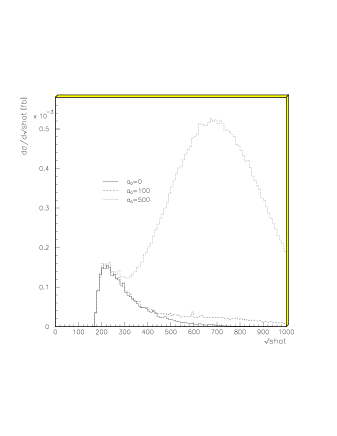
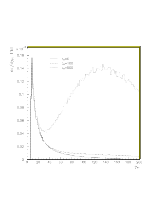
Figure 4: $\sqrt{\hat{s}}$ spectrum (left) and transverse photon energy spectrum (right) for the process $p\bar{p}\to W^{+}W^{-}\gamma$ in the presence of the anomalous coupling $a_{0}$.

In Figure 4 we also show the impact of the anomalous parameter $a_{0}$ on the transverse momentum of the photon. As anticipated above, it is the hard tail of the photon spectrum that is particularly sensitive to the anomalous contributions and this observable therefore offers a means to search directly for such anomalous contributions.

Finally, we have studied the impact on the total cross sections of the processes $p\bar{p}\to W^{+}W^{-}\gamma$ and $Z\gamma\gamma$. Figure 5 shows the contour in the $(a_{0},a_{c})$ plane corresponding to the $+3\sigma$ deviation of the SM cross section. Just as in the LEP2 study, $Z\gamma\gamma$ production promises a better discovery potential, again due to the higher photon energy available.

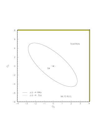
Figure 5: Contour plots for $+3\,\sigma$ deviations from the SM $p\bar{p}\to W^{+}W^{-}\gamma$ and $p\bar{p}\to Z^{0}\gamma\gamma$ total cross sections at $\sqrt{s}=2$ TeV with $\int{\cal L}=2$ fb^-1.

Comparing Figures 3 and 5, we conclude that the Tevatron should be able to set much tighter limits on the anomalous couplings $a_{0}$ and $a_{c}$ than LEP. The basic difference is the significantly higher subprocess scattering energies available at the hadron collider.

5 Measurements of anomalous couplings at hadron colliders

At $e^{+}e^{-}$ colliders anomalous couplings are directly investigated at a fixed centre of mass energy $\sqrt{s}$. This results in bounds of the anomalous couplings $\alpha_{\rm ac}$ as a function of $s$. At hadron colliders, the center of mass energy of the colliding partons $\sqrt{\hat{s}}$ is not fixed and there will be events where $\sqrt{\hat{s}}$ is very large. In order to avoid problems with violation of unitarity, form factors $f$ are introduced, i.e. the anomalous couplings $\alpha_{\rm ac}$ are replaced by $\alpha_{\rm ac}f$. The precise form of $f$ as well as the associated scale for new physics $\Lambda$ are to a big extent arbitrary. A common choice is

$$f=\left(1+\frac{\hat{s}}{\Lambda^{2}}\right)^{-n}$$ (8)

where $n$ is chosen big enough to ensure unitarity for $\hat{s}\to\infty$. This procedure has the unpleasant consequence that all bounds on the anomalous couplings depend on $\Lambda$ and the precise form of $f$.

In order to improve the situation it is desirable to get bounds directly on $\alpha_{\rm ac}(\sqrt{\hat{s}})$ also at hadron colliders. In some cases, this is straightforward to do. As an example we mention $Z\gamma$ production which probes the anomalous couplings $h_{3}^{\gamma},h_{4}^{\gamma},h_{3}^{Z}$ and $h_{4}^{Z}$. In this process $\hat{s}$ can be fully reconstructed. This allows to investigate the anomalous couplings in different regions of $\hat{s}$ and get separate bounds in each region. At the LHC the statistics should be good enough to allow such an analysis.

The situation is more difficult in processes, where $\hat{s}$ can not be fully reconstructed, such as $pp\to W\gamma\to\ell\nu\gamma X$. In these cases an observable quantity has to be found which has a very strong correlation to $\hat{s}$. Then the analysis could be done using this quantity instead of $\hat{s}$ without introducing a large error. There are several possibilities, such as the transverse mass $M_{T}$ or the cluster mass $M_{C}$. They are defined as follows:

$$M_{T}^{2} \equiv \biggl{(}\sqrt{p_{T}^{2}(\ell\gamma)+m^{2}(\ell\gamma)}+|p_{T}(\nu)|\biggl{)}^{2}-p_{T}^{2}(\ell\gamma\nu)$$ (9)

$$M_{C}^{2} \equiv \biggl{(}\sqrt{p_{T}^{2}(\ell\gamma)+m^{2}(\ell\gamma)}+|p_{T}(\nu)|\biggl{)}^{2}$$ (10)

Note that at leading order $M_{T}=M_{C}$. Another possibility is to take $\hat{s}_{\rm min}$ [11] which is defined as follows: assuming the $W$ to be on-shell and identifying the missing transverse momentum with $p_{T}(\nu)$ it is possible to reconstruct the full kinematics with a twofold ambiguity. This result in two possible values of $\hat{s}$ and $\hat{s}_{\rm min}$ is by definition the smaller of the two. In Figure 6 the distribution of the true $\hat{s}$ is shown for two particular bins of the observed quantity. The curves have been obtained for $pp$ collision at $\sqrt{s}$=14 TeV with some appropriate cuts on the rapidity and transverse momentum of the leptons. For plots (a) and (b) we have $150~{}{\rm GeV}<{\cal Q}<200~{}{\rm GeV}$ whereas for plots (c) and (d) we have $600~{}{\rm GeV}<{\cal Q}<650~{}{\rm GeV}$ where the observed quantity ${\cal Q}\in\{M_{T},M_{C},\hat{s}_{\rm min}\}$. To make the comparison of the various correlations easier, the histogram has been normalized to one in the first bin. The by far strongest correlations are obtained for $\hat{s}_{\rm min}$. Even if we include unrealistically large anomalous couplings the correlation is preserved, if not enhanced. This can be seen in Figures 6 (b) and (d), where we show the correlations with $\Delta\kappa^{\gamma}=0.8,\lambda=0.2$ and the ususal dipole form factor with a scale $\Lambda=1$ TeV. These results have been obtained with a Monte Carlo program including next-to-leading order QCD corrections [11]. The large correlation between $\hat{s}$ and $\hat{s}_{\rm min}$ should allow for a similar analysis as in the case of $Z\gamma$ production by simply replacing $\hat{s}$ by $\hat{s}_{\rm min}$.

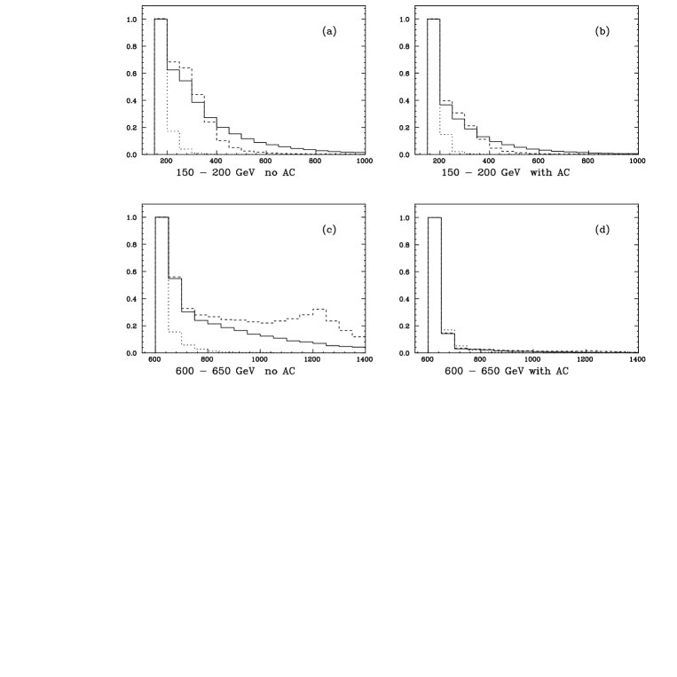
Figure 6: Correlation of $M_{T}$ (solid line), $M_{C}$ (dashed line) and $\hat{s}_{\rm min}$ (dotted line) with $\hat{s}$ for two bins in the observable for the LHC. Plots (a) and (c) are Standard Model results whereas plots (b) and (d) include large anomalous couplings.

References

References

- [1] Ellison J, Wudka J 1998 preprint hep-ph/9804322.
- [2] Hagiwara K et al. 1987 Nucl. Phys. B282 253.
- [3] Bilenky M, Kneur J L, Renard F M and Schildknecht D 1991 Nucl. Phys. 263 291.
- [4] Kobayashi M and Maskawa M 1973 Progr. Theor. Phys. 49, 652.
- [5] Gounaris G, Schildknecht D and Renard F M 1991 Phys. Lett. B263, 291.
- [6] Gounaris G, Papadopoulos C G 1998 Eur.Phys.J. C2 365.
- [7] Gounaris G, Layssac J, Moultaka G and Renard F M 1993 Int. J. Mod. Phys. A8 3285.
- [8] Bélanger G, Boudjema F 1992 Phys. Lett. 288 201.
-
[9]
Éboli O J P, Gonzaléz-Garcia M C, Novaes S F 1994
Nucl. Phys. B411 381;
Bélanger G et al. 1999 preprint hep-ph/9908254. - [10] Stirling W J, Werthenbach A 1999 preprint hep-ph/9903315, to appear in Euro. Phys. J.
- [11] de Florian D and Signer A 2000 preprint hep-ph/0002138.