Theory of Light Hydrogenlike Atoms

Abstract

The present status and recent developments in the theory of light hydrogenic atoms, electronic and muonic, are extensively reviewed. The discussion is based on the quantum field theoretical approach to loosely bound composite systems. The basics of the quantum field theoretical approach, which provide the framework needed for a systematic derivation of all higher order corrections to the energy levels, are briefly discussed. The main physical ideas behind the derivation of all binding, recoil, radiative, radiative-recoil, and nonelectromagnetic spin-dependent and spin-independent corrections to energy levels of hydrogenic atoms are discussed and, wherever possible, the fundamental elements of the derivations of these corrections are provided. The emphasis is on new theoretical results which were not available in earlier reviews. An up-to-date set of all theoretical contributions to the energy levels is contained in the paper. The status of modern theory is tested by comparing the theoretical results for the energy levels with the most precise experimental results for the Lamb shifts and gross structure intervals in hydrogen, deuterium, and helium ion $He^{+}$, and with the experimental data on the hyperfine splitting in muonium, hydrogen and deuterium.

Contents

toc

Part I

FIG. 1.: Hydrogen energy levels

Our goal here is to present a state of the art discussion of the theory of the Lamb shift and hyperfine splitting in light hydrogenlike atoms. In the body of the paper the spin independent corrections are discussed mainly as corrections to the hydrogen energy levels (see Fig. Contents), and the theory of hyperfine splitting is discussed in the context of the hyperfine splitting in the ground state of muonium (see Fig. 2). These two simple atomic systems are singled out for practical reasons, because highly precise experimental data exists in both cases, and the most accurate theoretical results are also obtained for these cases. However, almost all formulae in this review are valid also for other light hydrogenlike systems, and some of these other applications, including muonic atoms, will be discussed in the text as well. We will present all theoretical results in the field, with emphasis on more recent results which either were not discussed in sufficient detail in the previous theoretical reviews [bs, sy], or simply did not exist when the reviews were written. Our emphasis on the theory means that, besides presenting an exhaustive compendium of theoretical results, we will also try to present a qualitative discussion of the origin and magnitude of different corrections to the energy levels, to give, when possible, semiquantitative estimates of expected magnitudes, and to describe the main steps of the theoretical calculations and the new effective methods which were developed in recent years. We will not attempt to present a detailed comparison of theory with the latest experimental results, leaving this task to the experimentalists. We will use the experimental results only for illustrative purposes.

FIG. 2.: Muonium energy levels

The paper consists of three main parts. In the introductory part we briefly remind the reader of the main characteristic features of the bound state physics. Then follows a detailed discussion of the corrections to the energy levels which do not depend on the nuclear spin. The last third of the paper is devoted to a systematic discussion of the physics of hyperfine splitting. Different corrections to the energy levels are ordered with respect to the natural small parameters $\alpha$, $Z\alpha$, $m/M$ and nonelectrodynamic parameters like the ratio of the nucleon size to the radius of the first Bohr orbit. These parameters have a transparent physical nature in the light hydrogenlike atoms. Powers of $\alpha$ describe the order of quantum electrodynamic corrections to the energy levels, parameter $Z\alpha$ describes the order of relativistic corrections to the energy levels, and the small mass ratio of the light and heavy particles is responsible for the recoil effects beyond the reduced mass parameter present in a relativistic bound state. Corrections which depend both on the quantum electrodynamic parameter $\alpha$ and the relativistic parameter $Z\alpha$ are ordered in a series over $\alpha$ at fixed power of $Z\alpha$, contrary to the common practice accepted in the physics of highly charged ions with large $Z$. This ordering is more natural from the point of view of the nonrelativistic bound state physics, since all radiative corrections to a contribution of a definite order in the nonrelativistic expansion originate from the same distances and describe the same physics, while the radiative corrections to the different terms in nonrelativistic expansion over $Z\alpha$ of the same order in $\alpha$ are generated at vastly different distances and could have drastically different magnitudes.

A few remarks about our notation. All formulae below are written for the energy shifts. However, not energies but frequencies are measured in the spectroscopic experiments. The formulae for the energy shifts are converted to the respective expressions for the frequencies with the help of the De Broglie relationship $E=h\nu$. We will ignore the difference between the energy and frequency units in our theoretical discussion. Comparison of the theoretical expressions with the experimental data will always be done in the frequency units, since transition to the energy units leads to loss of accuracy. All numerous contributions to the energy levels in different sections of this paper are generically called $\Delta E$ and as a rule do not carry any specific labels, but it is understood that they are all different.

Let us mention briefly some of the closely related subjects which are not considered in this review. The physics of the high $Z$ ions is nowadays a vast and well developed field of research, with its own problems, approaches and tools, which in many respects are quite different from the physics of low $Z$ systems. We discuss below the numerical results obtained in the high $Z$ calculations only when they have a direct relevance for the low $Z$ atoms. The reader can find a detailed discussion of the high $Z$ physics in a number of recent reviews (see, e.g., [mps]). In trying to preserve a reasonable size of this review we decided to omit discussion of positronium, even though many theoretical expressions below are written in such form that for the case of equal masses they turn into respective corrections for the positronium energy levels. Positronium is qualitatively different from hydrogen and muonium not only due to the equality of the masses of its constituents, but because unlike the other light atoms there exists a whole new class of corrections to the positronium energy levels generated by the annihilation channel which is absent in other cases. Our discussion of the new theoretical methods will be incomplete due to omission of the recently developed and now popular nonrelativistic QED (NRQED) [caswelllep] which was especially useful in the positronium calculations, but was rarely used in the hydrogen and muonium physics. Very lucid presentations of NRQED exist in the recent literature (see, e.g., [kn10]).

PartII

-12

$\displaystyle\approx 1-\frac{(Z\alpha)^{2}}{2n^{2}}-\frac{(Z\alpha)^{4}}{2n^{3}}(\frac{1}{j+\frac{1}{2}}-\frac{3}{4n})-\frac{(Z\alpha)^{6}}{8n^{3}}\left[\frac{1}{(j+\frac{1}{2})^{3}}+\frac{3}{n(j+\frac{1}{2})^{2}}+\frac{5}{2n^{3}}-\frac{6}{n^{2}(j+\frac{1}{2})}\right]+\ldots,$

and $j=1/2,3/2,\ldots,n-1/2$ is the total angular momentum of the state.

In the Dirac spectrum, energy levels with the same principal quantum number $n$ but different total angular momentum $j$ are split into $n$ components of the fine structure, unlike the nonrelativistic Schrödinger spectrum where all levels with the same $n$ are degenerate. However, not all degeneracy is lifted in the spectrum of the Dirac equation: the energy levels corresponding to the same $n$ and $j$ but different $l=j\pm 1/2$ remain doubly degenerate. This degeneracy is lifted by the corrections connected with the finite size of the Coulomb source, recoil contributions, and by the dominating QED loop contributions. The respective energy shifts are called the Lamb shifts (see exact definition in Section LABEL:leadreclambdef) and will be one of the main subjects of discussion below. We would like to emphasize that the quantum mechanical (recoil and finite nuclear size) effects alone do not predict anything of the scale of the experimentally observed Lamb shift which is thus essentially a quantum electrodynamic (field-theoretical) effect.

One trivial improvement of the Dirac formula for the energy levels may easily be achieved if we take into account that, as was already discussed above, the electron motion in the Coulomb field is essentially nonrelativistic, and, hence, all contributions to the binding energy should contain as a factor the reduced mass of the electron-nucleus nonrelativistic system rather than the electron mass. Below we will consider the expression with the reduced mass factor

$$E_{nj}=m+m_{r}[f(n,j)-1],$$ (6)

rather than the naive expression in eq.(LABEL:naivdirac), as a starting point for calculation of corrections to the electron energy levels. In order to provide a solid starting point for further calculations the Dirac spectrum with the reduced mass dependence in eq.(6) should be itself derived from QED (see Section LABEL:leadreclambdef below), and not simply postulated on physical grounds as is done here.

III Bethe-Salpeter Equation and the Effective Dirac Equation

FIG. 3.: Bethe-Salpeter equation

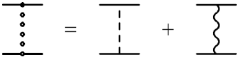
Quantum field theory provides an unambiguous way to find energy levels of any composite system. They are determined by the positions of the poles of the respective Green functions. This idea was first realized in the form of the Bethe-Salpeter (BS) equation for the two-particle Green function (see Fig. 3) [bethesalp]

$$\hat{G}=S_{0}+S_{0}K_{BS}\hat{G},$$ (7)

where $S_{0}$ is a free two-particle Green function, the kernel $K_{BS}$ is a sum of all two-particle irreducible diagrams in Fig. 4, and $\hat{G}$ is the total two-particle Green function.

FIG. 4.: Kernel of the Bethe-Salpeter equation

At first glance the field-theoretical BS equation has nothing in common with the quantum mechanical Schrödinger and Dirac equations discussed above. However, it is not too difficult to demonstrate that with selection of a certain subset of interaction kernels (ladder and crossed ladder), followed by some natural approximations, the BS eigenvalue equation reduces in the leading approximation, in the case of one light and one heavy constituent, to the Schrödinger or Dirac eigenvalue equations for a light particle in a field of a heavy Coulomb center. The basics of the BS equation are described in many textbooks (see, e.g., [blp, itzzub, fgross]), and many important results were obtained in the BS framework.

However, calculations beyond the leading order in the original BS framework tend to be rather complicated and nontransparent. The reasons for these complications can be traced to the dependence of the BS wave function on the unphysical relative energy (or relative time), absence of the exact solution in the zero-order approximation, non-reducibility of the ladder approximation to the Dirac equation, when the mass of the heavy particle goes to infinity, etc. These difficulties are generated not only by the nonpotential nature of the bound state problem in quantum field theory, but also by the unphysical classification of diagrams with the help of the notion of two-body reducibility. As it was known from the very beginning [bethesalp] there is a tendency to cancellation between the contributions of the ladder graphs and the graphs with crossed photons. However, in the original BS framework, these graphs are treated in profoundly different ways. It is quite natural, therefore, to seek such a modification of the BS equation, that the crossed and ladder graphs play a more symmetrical role. One also would like to get rid of other drawbacks of the original BS formulation, preserving nevertheless its rigorous field-theoretical contents.

The BS equation allows a wide range of modifications since one can freely modify both the zero-order propagation function and the leading order kernel, as long as these modifications are consistently taken into account in the rules for construction of the higher order approximations, the latter being consistent with eq.(7) for the two-particle Green function. A number of variants of the original BS equation were developed since its discovery (see, e.g.,[gy1, gy2, fgr, dulf, lep]). The guiding principle in almost all these approaches was to restructure the BS equation in such a way, that it would acquire a three-dimensional form, a soluble and physically natural leading order approximation in the form of the Schrödinger or Dirac equations, and more or less transparent and regular way for selection of the kernels relevant for calculation of the corrections of any required order.

We will describe, in some detail, one such modification, an effective Dirac equation (EDE) which was derived in a number of papers [gy2, fgr, dulf, lep]. This new equation is more convenient in many applications than the original BS equation, and we will derive some general formulae connected with this equation. The physical idea behind this approach is that in the case of a loosely bound system of two particles of different masses, the heavy particle spends almost all its life not far from its own mass shell. In such case some kind of Dirac equation for the light particle in an external Coulomb field should be an excellent starting point for the perturbation theory expansion. Then it is convenient to choose the free two-particle propagator in the form of the product of the heavy particle mass shell projector $\Lambda$ and the free electron propagator

$$\Lambda S(p,l,E)=2\pi i\delta^{(+)}(p^{2}-M^{2})\frac{p/+M}{E-p/-m}(2\pi)^{4}\delta^{(4)}(p-l)$$ (8)

where $p_{\mu}$ and $l_{\mu}$ are the momenta of the incoming and outgoing heavy particle, $E_{\mu}-p_{\mu}$ is the momentum of the incoming electron ($E=(E,{\bf 0})$ - this is the choice of the reference frame), and $\gamma$-matrices associated with the light and heavy particles act only on the indices of the respective particle.

The free propagator in eq.(8) determines other building blocks and the form of a two-body equation equivalent to the BS equation, and the regular perturbation theory formulae in this case were obtained in [dulf, lep].

In order to derive these formulae let us first write the BS equation in eq.(7) in an explicit form

$$\hat{G}(p,l,E)=S_{0}(p,l,E)+\int\frac{d^{4}k}{(2\pi)^{4}}\int\frac{d^{4}q}{(2\pi)^{4}}S_{0}(p,k,E)K_{BS}(k,q,E)\hat{G}(q,l,E),$$ (9)

where

$$S_{0}(p,k,E)=\frac{i}{p/-M}\frac{i}{E-l/-m}(2\pi)^{4}\delta^{(4)}(p-l).$$ (10)

The amputated two-particle Green function $G_{T}$ satisfies the equation

$$G_{T}=K_{BS}+K_{BS}S_{0}G_{T},$$ (11)

A new kernel corresponding to the free two-particle propagator in eq.(8) may be defined via this amputated two-particle Green function

$$G_{T}=K+K\Lambda SG_{T}.$$ (12)

Comparing eq.(11) and eq.(12) one easily obtains the diagrammatic series for the new kernel $K$ (see Fig. 5)

$$K(q,l,E)=[I-K_{BS}(S_{0}-\Lambda S)]^{-1}K_{BS}=K_{BS}(q,l,E)+$$ (13)

$\displaystyle\int\frac{d^{4}r}{(2\pi)^{4}}K_{BS}(q,r,E)\left\{\frac{i}{r/-M}\frac{i}{E-r/-m}-2\pi i\delta^{(+)}(r^{2}-M^{2})\frac{r/+M}{E-r/-m}\right\}K_{BS}(r,l,E)+\ldots.$

FIG. 5.: Series for the kernel of the Effective Dirac equation

The new bound state equation is constructed for the two-particle Green function defined by the relationship

$$G=\Lambda S+\Lambda SG_{T}\Lambda S.$$ (14)

The two-particle Green function $G$ has the same poles as the initial Green function $\hat{G}$ and satisfies the BS-like equation

$$G=\Lambda S+\Lambda SKG,$$ (15)

or, explicitly,

$$G(p,l,E)=2\pi i\delta^{(+)}(p^{2}-M^{2})\frac{p/+M}{E-p/-m}(2\pi)^{4}\delta^{(4)}(p-l)$$ (16)

$\displaystyle+2\pi i\delta^{(+)}(p^{2}-M^{2})\frac{p/+M}{E-p/-m}\int\frac{d^{4}q}{(2\pi)^{4}}K(p,q,E)G(q,l,E).$

This last equation is completely equivalent to the original BS equation, and may be easily written in a three-dimensional form

$$\widetilde{G}({\bf p},{\bf l},E)=\frac{p/+M}{E-p/-m}\left\{(2\pi)^{3}\delta^{(3)}({\bf p-l})+\int\frac{d^{3}q}{(2\pi)^{3}2E_{q}}iK({\bf p},{\bf q},E)\widetilde{G}({\bf q},{\bf l},E)\right\},$$ (17)

where all four-momenta are on the mass shell $p^{2}=l^{2}=q^{2}=M^{2}$, $E_{q}=\sqrt{{\bf p}^{2}+M^{2}}$, and the three-dimensional two-particle Green function $\widetilde{G}$ is defined as follows

$$G(p,l,E)=2\pi i\delta^{(+)}(p^{2}-M^{2})\widetilde{G}({\bf p},{\bf l},E)2\pi i\delta^{(+)}(l^{2}-M^{2}).$$ (18)

Taking the residue at the bound state pole with energy $E_{n}$ we obtain a homogeneous equation

$$(E/_{n}-p/-m)\phi({\bf p},E_{n})=(p/+M)\int\frac{d^{3}q}{(2\pi)^{3}2E_{q}}iK({\bf p},{\bf q},E_{n})\phi({\bf q},E_{n})$$ (19)

Due to the presence of the heavy particle mass shell projector on the right hand side the wave function in eq.(19) satisfies a free Dirac equation with respect to the heavy particle indices

$$(p/-M)\phi({\bf p},E_{n})=0.$$ (20)

Then one can extract a free heavy particle spinor from the wave function in eq.(19)

$$\phi({\bf p},E_{n})=\sqrt{2E_{n}}U({\bf p})\psi({\bf p},E_{n})$$ (21)

where

$$U({\bf p})=\left(\begin{array}[]{rc}\sqrt{E_{p}+M}&I\\ \sqrt{E_{p}-M}&\frac{\boldmath\mbox{$p\cdot\sigma$}}{|{\boldmath\mbox{$p$}}|}\end{array}\right).$$ (22)

Finally, the eight-component wave function $\psi({\bf p},E_{n})$ (four ordinary electron spinor indices, and two extra indices corresponding to the two-component spinor of the heavy particle) satisfies the effective Dirac equation (see Fig. 6)

$$(E/_{n}-p/-m)\psi({\bf p},E_{n})=\int\frac{d^{3}q}{(2\pi)^{3}2E_{q}}i\widetilde{K}({\bf p},{\bf q},E_{n})\psi({\bf q},E_{n}),$$ (23)

where

$$\widetilde{K}({\bf p},{\bf q},E_{n})=\frac{\bar{U}({\bf p})K({\bf p},{\bf q},E_{n})U({\bf q})}{\sqrt{4E_{p}E_{q}}},$$ (24)

$k=(E_{n}-p_{0},-{\bf p})$ is the electron momentum, and the crosses on the heavy line in Fig. 6 mean that the heavy particle is on its mass shell.

FIG. 6.: Effective Dirac equation

The inhomogeneous equation eq.(17) also fixes the normalization of the wave function.

Even though the total kernel in eq.(23) is unambiguously defined, we still have freedom to choose the zero-order kernel $K_{0}$ at our convenience, in order to obtain a solvable lowest order approximation. It is not difficult to obtain a regular perturbation theory series for the corrections to the zero-order approximation corresponding to the difference between the zero-order kernel $K_{0}$ and the exact kernel $K_{0}+\delta K$

$$E_{n}=E_{n}^{0}+(n|i\delta K(E_{n}^{0})|n)\left(1+(n|i\delta K^{\prime}(E_{n}^{0})|n)\right)$$ (25)

$\displaystyle+(n|i\delta K(E_{n}^{0})G_{n0}(E_{n}^{0})i\delta K(E_{n}^{0})|n)\left(1+(n|i\delta K^{\prime}(E_{n}^{0})|n)\right)+\dots,$

where the summation of intermediate states goes with the weight $d^{3}p/[(2\pi)^{3}2E_{p}]$ and is realized with the help of the subtracted free Green function of the EDE with the kernel $K_{0}$

$$G_{n0}(E)=G_{0}(E)-\frac{|n)(n|}{E-E_{n}^{0}},$$ (26)

conjugation is understood in the Dirac sense, and $\delta K^{\prime}(E_{n}^{0})\equiv(dK/dE)_{|E=E_{n}^{0}}$.

The only apparent difference of the EDE eq.(23) from the regular Dirac equation is connected with the dependence of the interaction kernels on energy. Respectively the perturbation theory series in eq.(25) contain, unlike the regular nonrelativistic perturbation series, derivatives of the interaction kernels over energy. The presence of these derivatives is crucial for cancellation of the ultraviolet divergences in the expressions for the energy eigenvalues.

A judicious choice of the zero-order kernel (sum of the Coulomb and Breit potentials, for more detail see, e.g, [gy1, gy2, lep]) generates a solvable unperturbed EDE in the external Coulomb field in Fig. 7. The eigenfunctions of this equation may be found exactly in the form of the Dirac-Coulomb wave functions (see, e.g, [lep]). For practical purposes it is often sufficient to approximate these exact wave functions by the product of the Schrödinger-Coulomb wave functions with the reduced mass and the free electron spinors which depend on the electron mass and not on the reduced mass. These functions are very convenient for calculation of the high order corrections, and while below we will often skip some steps in the derivation of one or another high order contribution from the EDE, we advise the reader to keep in mind that almost all calculations below are done with these unperturbed wave functions.

FIG. 7.: Effective Dirac equation in the external Coulomb field

Part III

FIG. 8.: Leading order contribution to the electron radius

The finite radius of the electron generates a correction to the Coulomb potential (see, e.g., [bd])

$$\delta V=\frac{1}{6}<r^{2}>\Delta V=\frac{2\pi}{3}Z\alpha<r^{2}>\delta({\bf r}),$$ (29)

where $V=-Z\alpha/r$ is the Coulomb potential.

The respective correction to the energy levels is simply given by the matrix element of this perturbation. Thus we immediately discover that the finite size of the electron produced by the QED radiative corrections leads to a shift of the hydrogen energy levels. Moreover, since this perturbation is nonvanishing only at the source of the Coulomb potential, it influences quite differently the energy levels with different orbital angular momenta, and, hence, leads to splitting of the levels with the same total angular momenta but different orbital momenta. This splitting lifts the degeneracy in the spectrum of the Dirac equation in the Coulomb field, where the energy levels depend only on the principal quantum number $n$ and the total angular momentum $j$.

It is very easy to estimate this splitting (shift of the $S$ level energy)

$$\Delta E=<nS|\delta V|nS>\approx|\Psi_{n}(0)|^{2}\frac{2\pi(Z\alpha)}{3}<r^{2}>$$ (30)

$\displaystyle\approx\frac{4m(Z\alpha)^{4}}{n^{3}}\frac{\alpha}{3\pi}\ln[(Z\alpha)^{-2}]\delta_{l0}\;{}_{{}_{|n=2}}\approx 1330~{}\mbox{MHz}.$

This result should be compared with the experimental number of about $1040$ MHz and the agreement is satisfactory for such a crude estimate. There are two qualitative features of this result to which we would like to attract the reader’s attention. First, the sign of the energy shift may be obtained without calculation. Due to the finite radius of the electron its charge in the $S$ state is on the average more spread out around the Coulomb source than in the case of the pointlike electron. Hence, the binding is weaker than in the case of the pointlike electron and the energy of the level is higher. Second, despite the presence of nonlogarithmic contributions missing in our crude calculation, their magnitude is comparatively small, and the logarithmic term above is responsible for the main contribution to the Lamb shift. This property is due to the would be infrared divergence of the considered contribution, which is cutoff by the small (in comparison with the electron mass) binding energy. As we will see below, whenever a correction is logarithmically enhanced, the respective logarithm gives a significant part of the correction, as is the case above.

FIG. 9.: Leading order polarization insertion

Another obvious contribution to the Lamb shift of the same leading order is connected with the polarization insertion in the photon propagator (see Fig. 9). This correction also induces a correction to the Coulomb potential

$$\delta V=-\frac{\Pi(-{\bf k}^{2})}{{\bf k}^{4}}_{|{\bf k}^{2}=0}\Delta V=\frac{\alpha}{15\pi m^{2}}\Delta V=-\frac{4}{15}\frac{\alpha(Z\alpha)}{m^{2}}\delta({\bf r}),$$ (31)

and the respective correction to the $S$-level energy is equal to

$$\Delta E=<nS|\delta V|nS>=-|\Psi_{n}(0)|^{2}\frac{4\alpha(Z\alpha)}{15m^{2}}$$ (32)

$\displaystyle=-\frac{4m(Z\alpha)^{4}}{n^{3}}\frac{\alpha}{15\pi}\delta_{l0}\;{}_{{}_{|n=2}}\approx-30~{}\mbox{MHz}.$

Once again the sign of this correction is evident in advance. The polarization correction may be thought of as a correction to the electric charge of the nucleon induced by the fact that the electron sees the proton from a finite distance. This means that the electron, which has penetrated in the polarization cloud, sees effectively a larger charge and experiences a stronger binding force, which lowers the energy level. Experimental observation of this contribution to the Lamb shift played an important role in the development of modern quantum electrodynamics since it explicitly confirmed the very existence of the closed electron loops. Numerically vacuum polarization contribution is much less important than the contribution connected with the electron spreading due to quantum corrections, and the total shift of the level is positive.

VI Natural Magnitudes of Corrections to the Lamb Shift

Let us emphasize that the main contribution to the Lamb shift is a radiative correction itself (compare eq.(30),eq.(32)) and contains a logarithmic enhancement factor. This is extremely important when one wants to get a qualitative understanding of the magnitude of the higher order corrections to the Lamb shift discussed below. Due to the presence of this accidental logarithmic enhancement it is impossible to draw conclusions about the expected magnitude of higher order corrections to the Lamb shift simply by comparing them to the magnitude of the leading order contribution. It is more reasonable to extract from this leading order contribution the term which can be called the skeleton factor and to use it further as a normalization factor. Let us write the leading order contributions in eq.(30),eq.(32) obtained above in the form

$$\frac{4m(Z\alpha)^{4}}{n^{3}}\times\mbox{\sl radiative correction},$$ (33)

where the radiative correction is either the slope of the Dirac form factor, roughly speaking equal to $m^{2}{dF_{1}(-{\bf k}^{2})}/{d{\bf k}^{2}}_{|{\bf k}^{2}=0}=\alpha/(3\pi)\ln(Z\alpha)^{-2}$, or the polarization correction $m^{2}{\Pi(-{\bf k}^{2})}/{{\bf k}^{4}}_{|{\bf k}^{2}=0}={\alpha}/({15\pi})$.

It is clear now that the scale setting factor which should be used for qualitative estimates of the high order corrections to the Lamb shift is equal to $4m(Z\alpha)^{4}/n^{3}$. Note the characteristic dependence on the principal quantum number $1/n^{3}$ which originates from the square of the wave function at the origin $|\psi(0)|^{2}\sim 1/n^{3}$. All corrections induced at small distances (or at high virtual momenta) have this characteristic dependence and are called state-independent. Even the coefficients before the leading powers of the low energy logarithms $\ln(Z\alpha)^{2}$ are state-independent since these leading logarithms originate from integration over the wide intermediate momenta region from $m(Z\alpha)^{2}$ to $m$, and the respective factor before the logarithm is determined by the high momenta part of the integration region. Estimating higher order corrections to the Lamb shift it is necessary to remember, as mentioned above, that unlike the case of radiative corrections to the scattering amplitudes, in the bound state problem factors $Z\alpha$ are not accompanied by an extra factor $\pi$ in the denominator. This well known feature of the Coulomb problem provides one more reason to preserve $Z$ in analytic expressions (even when $Z=1$), since in this way one may easily separate powers of $Z\alpha$ not accompanied by $\pi$ from powers of $\alpha$ which always enter formulae in the combination $\alpha/\pi$.

PartIV⋅

$\displaystyle\sigma$.

A simplified derivation of the Breit interaction potential may be found in many textbooks (see, e.g., [blp]).

All contributions to the energy levels up order $(Z\alpha)^{4}$ may be calculated from the total Breit Hamiltonian

$$H_{Br}=H_{0}+V_{Br},$$ (36)

where the interaction potential is the sum of the instantaneous Coulomb and Breit potentials in Fig. 10.

FIG. 10.: Sum of the Coulomb and Breit kernels

The corrections of order $(Z\alpha)^{4}$ are just the first order matrix elements of the Breit interaction between the Coulomb-Schrödinger eigenfunctions of the Coulomb Hamiltonian $H_{0}$ in eq.(LABEL:twopartcoul). The mass dependence of the Breit interaction is known exactly, and the same is true for its matrix elements. These matrix elements and, hence, the exact mass dependence of the contributions to the energy levels of order $(Z\alpha)^{4}$, beyond the reduced mass, were first obtained a long time ago [bg]

$$E_{nj}^{tot}=(m+M)-\frac{m_{r}(Z\alpha)^{2}}{2n^{2}}-\frac{m_{r}(Z\alpha)^{4}}{2n^{3}}\left(\frac{1}{j+\frac{1}{2}}-\frac{3}{4n}+\frac{m_{r}}{4n(m+M)}\right)$$ (37)

$\displaystyle+\frac{(Z\alpha)^{4}m_{r}^{3}}{2n^{3}M^{2}}\left(\frac{1}{j+\frac{1}{2}}-\frac{1}{l+\frac{1}{2}}\right)(1-\delta_{l0}).$

Note the emergence of the last term in eq.(37) which lifts the characteristic degeneracy in the Dirac spectrum between levels with the same $j$ and $l=j\pm 1/2$. This means that the expression for the energy levels in eq.(37) already predicts a nonvanishing contribution to the classical Lamb shift $E(2S_{\frac{1}{2}})-E(2P_{\frac{1}{2}})$. Due to the smallness of the electron-proton mass ratio this extra term is extremely small in hydrogen. The leading contribution to the Lamb shift, induced by the QED radiative correction, is much larger.

In the Breit Hamiltonian in eq.(LABEL:breitpot) we have omitted all terms which depend on spin variables of the heavy particle. As a result the corrections to the energy levels in eq.(37) do not depend on the relative orientation of the spins of the heavy and light particles (in other words they do not describe hyperfine splitting). Moreover, almost all contributions in eq.(37) are independent not only of the mutual orientation of spins of the heavy and light particles but also of the magnitude of the spin of the heavy particle. The only exception is the small contribution proportional to the term $\delta_{l0}$, called the Darwin-Foldy contribution. This term arises in the matrix element of the Breit Hamiltonian only for the spin one-half nucleus and should be omitted for spinless or spin one nuclei. This contribution combines naturally with the nuclear size correction, and we postpone its discussion to Section XVII B dealing with the nuclear size contribution.

In the framework of the effective Dirac equation in the external Coulomb field (see Fig. 7) the result in eq.(37) was first obtained in [gy1] (see also [gy2, lep]) and rederived once again in [sy], where it was presented in the form

$$E_{nj}^{tot}=(m+M)+m_{r}[f(n,j)-1]-\frac{m_{r}^{2}}{2(m+M)}[f(n,j)-1]^{2}$$ (38)

$\displaystyle+\frac{(Z\alpha)^{4}m_{r}^{3}}{2n^{3}M^{2}}\left(\frac{1}{j+\frac{1}{2}}-\frac{1}{l+\frac{1}{2}}\right)(1-\delta_{l0}).$

This equation has the same contributions of order $(Z\alpha)^{4}$ as in eq.(37), but formally this expression also contains nonrecoil and recoil corrections of order $(Z\alpha)^{6}$ and higher. The nonrecoil part of these contributions is definitely correct since the Dirac energy spectrum is the proper limit of the spectrum of a two-particle system in the nonrecoil limit $m/M=0$. As we will discuss later the first-order mass ratio contributions in eq.(38) correctly reproduce recoil corrections of higher orders in $Z\alpha$ generated by the Coulomb and Breit exchange photons. Additional first order mass ratio recoil contributions of order $(Z\alpha)^{6}$ will be calculated below. Recoil corrections of order $(Z\alpha)^{8}$ were never calculated and at the present stage the mass dependence of these terms should be considered as completely unknown.

Recoil corrections depending on odd powers of $Z\alpha$ are also missing in eq.(38), since as was explained above all corrections generated by the one-photon exchange necessarily depend on the even powers of $Z\alpha$. Hence, to calculate recoil corrections of order $(Z\alpha)^{5}$ one has to consider the nontrivial contribution of the box diagram. We postpone discussion of these corrections until Section LABEL:lambreczalpha5.

It is appropriate to give an exact definition of what is called the Lamb shift. In the early days of the Lamb shift studies, experimentalists measured not a shift but the classical Lamb splitting $E(2S_{\frac{1}{2}})-E(2P_{\frac{1}{2}})$ between the energy levels which are degenerate according to the naive Dirac equation in the Coulomb field. This splitting is an experimental observable defined independently of any theory. Modern experiments now produce high precision experimental data for the nondegenerate $1S$ energy level, and the very notion of the Lamb shift in this case, as well as in the case of an arbitrary energy level, does not admit an unambiguous definition. It is most natural to call the Lamb shift the sum of all contributions to the energy levels which lift the double degeneracy of the Dirac-Coulomb spectrum with respect to $l=j\pm 1/2$ (see Section LABEL:diraccoul). There emerged an almost universally adopted convention to call the Lamb shift the sum of all contributions to the energy levels beyond the first three terms in eq.(38) and excluding, of course, all hyperfine splitting contributions. This means that we define the Lamb shift by the relationship

$$E_{njl}^{tot}=(m+M)+m_{r}[f(n,j)-1]-\frac{m_{r}^{2}}{2(m+M)}[f(n,j)-1]^{2}+L_{njl}\equiv E_{nj}^{DR}+L_{njl}.$$ (39)

We will adopt this definition below.

VIII Radiative Corrections of Order $\alpha^{n}(Z\alpha)^{4}m$

Let us turn now to the discussion of radiative corrections which may be calculated in the external field approximation.

A Leading Contribution to the Lamb Shift

1 Radiative Insertions in the Electron line and the Dirac Form Factor Contribution

The main contribution to the Lamb shift was first estimated in the nonrelativistic approximation by Bethe [bethe], and calculated by Kroll and Lamb [kl], and by French and Weisskopf [fw]. We have already discussed above qualitatively the nature of this contribution. In the effective Dirac equation framework the apparent perturbation kernels to be taken into account are the diagrams with the radiative photon spanning any number of the exchanged Coulomb photons in Fig. III and Fig. 11. The dominant logarithmic contribution to the Lamb shift is produced by the slope of the Dirac form factor $F_{1}$, but superficially all these kernels can lead to corrections of order $\alpha(Z\alpha)^{4}$ and one cannot discard any of them. An additional problem is connected with the infrared divergence of the kernels on the mass shell. There cannot be any true infrared divergence in the bound state problem since all would be infrared divergences are cut off either at the inverse Bohr radius or by the electron binding energy. Nevertheless such spurious on-shell infrared divergences can complicate the calculations.

FIG. 11.: Kernels with many spanned Coulomb photons

An important step which greatly facilitates treatment of all these problems consists in separation of the radiative photon integration region with the help of auxiliary parameter $\sigma$ in such way that $m(Z\alpha)^{2}\ll\sigma\ll m(Z\alpha)$. It is easy to see that in the high momentum region each additional Coulomb photon produces an extra factor $Z\alpha$, so it is sufficient to consider only the kernel with one Coulomb photon in this region. Moreover, the auxiliary parameter $\sigma$ provides an infrared cutoff for the vertex graph and thus solves the problem of the would be infrared divergence. Due to the choice of the parameter $\sigma\gg m(Z\alpha)^{2}$ one may ignore the binding energy in the high momentum region. The main contribution to the Lamb shift is induced by the Dirac form factor $F_{1}(k^{2})-1$ which is proportional to the transferred momentum squared at small momentum transfer. This transferred momentum squared factor exactly cancels the Coulomb photon propagator attached to the Dirac form factor, and momentum space integrations over wave function momenta factorize, thereby producing the wave function squared at the origin in the coordinate space. It is clear that if one would take into account the small virtuality of either external electron line, expanding the integrand in this virtuality, it would lead to an extra factor of momentum squared in the integrand, and after integration with the wave function would lead to an extra factor $(Z\alpha)^{2}$ in the contribution to the energy shift. Hence, since we are interested in the contribution of order $\alpha(Z\alpha)^{4}$, we may freely ignore the virtuality of the electron line in the kernel in the high momentum region. It is also clear even at this stage, that the high momentum region does not produce any contribution for the non-$S$ states because the wave function vanishes at the origin for such states, and, hence, the logarithmic contribution is missing for the non-$S$ states.

Of course, all approximations made above are invalid in the low momentum integration region, where one cannot consider only the kernel with the radiative photon spanning only one Coulomb exchange. For soft radiative photons with characteristic momenta of order $m(Z\alpha)^{2}$ graphs with any number of spanned exchanged photons in Fig. 11 have the same order of magnitude and one has to take these graphs into account simultaneously. This means that one has to calculate the matrix element of the exact self-energy operator in the external Coulomb field between Dirac-Coulomb wave functions. This problem may seem formidable at first sight, but it can be readily solved with the help of old-fashioned perturbation theory by inserting a complete set of intermediate states and performing calculations in the dipole approximation, which is adequate to accuracy $\alpha(Z\alpha)^{4}m$. It should be mentioned that the magnitude of the upper boundary of the interval for the auxiliary parameter $\sigma$ was chosen in order to provide validity of the dipole approximation.

The most important fact about the auxiliary parameter $\sigma$ is that one can use different approximations for calculations of the high- and low-momentum contributions. In the high-momentum region the factor $m(Z\alpha)^{2}/k\leq(m(Z\alpha)^{2}/\sigma\ll 1$ plays the role of a small parameter and one can consider binding effects as small corrections. In the low-momentum region $k/(mZ\alpha)\leq\sigma/(mZ\alpha)\ll 1$ one may use the nonrelativistic multipole expansion, and the main contribution in this region is given by the dipole contribution. The crucial point is that for $k\sim\sigma$ both expansions are valid simultaneously and one can match them without loss in accuracy. Matching the high- and low-momentum contributions one obtains the classical result for the shift of the energy level generated by the slope of the Dirac form factor

$$\Delta E=\left\{\left[\frac{1}{3}\ln\frac{m(Z\alpha)^{-2}}{m_{r}}+\frac{11}{72}\right]\delta_{l0}-\frac{1}{3}\ln k_{0}(n,l)\right\}\frac{4\alpha(Z\alpha)^{4}}{\pi n^{3}}\left(\frac{m_{r}}{m}\right)^{3}m,$$ (40)

where $m_{r}=mM/(m+M)$ is the reduced mass and $\ln k_{0}(n,l)$ is the so called Bethe logarithm. The factor $m/m_{r}$ arises in the argument of the would be infrared divergent logarithm $\ln(m/\lambda)$ since in the nonrelativistic approximation the energy levels of an atom depend only on the reduced mass and, hence, the infrared divergence is cut off by the binding energy $m_{r}(Z\alpha)^{2}$ [sy].

The mass dependence of the correction of order $\alpha(Z\alpha)^{4}$ beyond the reduced mass factor is properly described by the expression in eq.(40) as was proved in [bg85, bg87]. In the same way as for the case of the leading relativistic correction in eq.(37), the result in eq.(40) is exact in the small mass ratio $m/M$, since in the framework of the effective Dirac equation all corrections of order $(Z\alpha)^{4}$ are generated by the kernels with one-photon exchange. In some earlier papers the reduced mass factors in eq.(40) were expanded up to first order in the small mass ratio $m/M$. Nowadays it is important to preserve an exact mass dependence in eq.(40) because current experiments may be able to detect quadratic mass corrections (about $2$ kHz for the $1S$ level in hydrogen) to the leading nonrecoil Lamb shift contribution.

The Bethe logarithm is formally defined as a certain normalized infinite sum of matrix elements of the coordinate operator over the Schrödinger-Coulomb wave functions. It is a pure number which can in principle be calculated with arbitrary accuracy, and high accuracy results for the Bethe logarithm can be found in the literature (see, e.g. [hm, drakeswain] and references therein). For convenience we have collected some values for the Bethe logarithms [drakeswain] in Table I.

Table I. Bethe Logarithms for some Lower Levels [drakeswain]

	$\ln k_{0}(n,l)$	$\Delta E=-\frac{4}{3}\ln k_{0}(n,l)\frac{\alpha(Z\alpha)^{4}}{\pi n^{3}}(\frac{m_{r}}{m})^{3}m$ kHz
$1S$	$2.984~{}128~{}555~{}765~{}498$	$-23~{}591.92$
$2S$	$2.811~{}769~{}893~{}120~{}563$	$-2~{}778.66$
$2P$	$-0.030~{}016~{}708~{}630~{}213$	$29.66$
$3S$	$2.767~{}663~{}612~{}491~{}822$	$-810.39$
$3P$	$-0.038~{}190~{}229~{}385~{}312$	$11.18$
$3D$	$-0.005~{}232~{}148~{}140~{}883$	$1.53$
$4S$	$2.749~{}811~{}840~{}454~{}057$	$-339.68$
$4P$	$-0.041~{}954~{}894~{}598~{}086$	$5.18$
$4D$	$-0.006~{}740~{}938~{}876~{}975$	$0.83$
$4F$	$-0.001~{}733~{}661~{}482~{}126$	$0.21$
$5S$	$2.740~{}823~{}727~{}854~{}572$	$-173.35$
$5P$	$-0.044~{}034~{}695~{}591~{}878$	$2.79$
$5D$	$-0.007~{}600~{}751~{}257~{}947$	$0.48$
$5F$	$-0.002~{}202~{}168~{}381~{}486$	$0.14$
$5G$	$-0.000~{}772~{}098~{}901~{}537$	$0.05$
$6S$	$2.735~{}664~{}206~{}935~{}105$	$-100.13$
$6P$	$-0.045~{}312~{}197~{}688~{}974$	$1.66$
$6D$	$-0.008~{}147~{}203~{}962~{}354$	$0.30$
$6F$	$-0.002~{}502~{}179~{}760~{}279$	$0.09$
$6G$	$-0.000~{}962~{}797~{}424~{}841$	$0.04$
$6H$	$-0.000~{}407~{}926~{}168~{}297$	$0.01$
$7S$	$2.732~{}429~{}129~{}187~{}092$	$-62.98$
$7P$	$-0.046~{}155~{}177~{}262~{}915$	$1.06$
$7D$	$-0.008~{}519~{}223~{}293~{}658$	$0.20$
$7F$	$-0.002~{}709~{}095~{}727~{}000$	$0.06$
$7G$	$-0.001~{}094~{}472~{}739~{}370$	$0.03$
$7H$	$-0.000~{}499~{}701~{}854~{}766$	$0.01$
$7I$	$-0.000~{}240~{}908~{}258~{}717$	$0.01$
$8S$	$2.730~{}267~{}260~{}690~{}589$	$-42.16$
$8P$	$-0.046~{}741~{}352~{}003~{}557$	$0.72$
$8D$	$-0.008~{}785~{}042~{}984~{}125$	$0.14$
$8F$	$-0.002~{}859~{}114~{}559~{}296$	$0.04$
$8G$	$-0.001~{}190~{}432~{}043~{}318$	$0.02$
$8H$	$-0.000~{}566~{}532~{}724~{}12$	$0.01$
$8I$	$-0.000~{}290~{}426~{}172~{}391$
$8K$	$-0.000~{}153~{}864~{}500~{}961$

2 Pauli Form Factor Contribution

The Pauli form factor $F_{2}$ also generates a small contribution to the Lamb shift. This form factor does not produce any contribution if one neglects the lower components of the unperturbed wave functions, since the respective matrix element is identically zero between the upper components in the standard representation for the Dirac matrices which we use everywhere. Taking into account lower components in the nonrelativistic approximation we easily obtain an explicit expression for the respective perturbation

$$\delta V=-\frac{1}{4m^{2}}\left[\Delta V+2~{}\mbox{\boldmath$\sigma$}~{}\frac{m}{m_{r}}~{}[\mbox{\boldmath$\nabla$}V\times{\bf p}]\right]F_{2}(0),$$ (41)

where $V=-Z\alpha/r$ is the Coulomb potential. Note the appearance of an extra factor $m/m_{r}$ in the coefficient before the second term. This is readily obtained from an explicit consideration of the radiatively corrected one photon exchange. In momentum space the term with the Laplacian of the Coulomb potential depends only on the exchanged momentum, while the second term contains explicit dependence on the electron momentum. Since the Pauli form factor depends explicitly on the electron momentum and not on the relative momentum of the electron-proton system, the transition to relative momentum, which is the argument of the unperturbed wave functions, leads to emergence of an extra factor $m/m_{r}$.

The interaction potential above generated by the Pauli form factor may be written in terms of the spin-orbit interaction

$$\delta V=\left[\frac{Z\alpha\pi}{m^{2}}\delta^{3}({\bf r})+\frac{Z\alpha\pi}{r^{3}mm_{r}}({\bf s}{\bf l})\right]~{}F_{2}(0),$$ (42)

where

$${\bf s}=\frac{\mbox{\boldmath$\sigma$}}{2},\;\;\;\;{\bf l}={\bf r}\times{\bf p}.$$ (43)

The respective contributions to the Lamb shift are given by

$$\Delta E_{|l=0}=\frac{(Z\alpha)^{4}m}{n^{3}}F_{2}(0)\left(\frac{m_{r}}{m}\right)^{3}=\frac{\alpha(Z\alpha)^{4}m}{2\pi n^{3}}\left(\frac{m_{r}}{m}\right)^{3},$$ (44)

$\displaystyle\Delta E_{|l\neq 0}=\frac{(Z\alpha)^{4}m}{n^{3}}F_{2}(0)\frac{j(j+1)-l(l+1)-3/4}{l(l+1)(2l+1)}\left(\frac{m_{r}}{m}\right)^{2}$

$\displaystyle=\frac{\alpha(Z\alpha)^{4}m}{2\pi n^{3}}\frac{j(j+1)-l(l+1)-3/4}{l(l+1)(2l+1)}\left(\frac{m_{r}}{m}\right)^{2},$

where we have used the Schwinger value [sch] of the anomalous magnetic moment $F_{2}(0)=\alpha/(2\pi)$. Correct reduced mass factors have been retained in this expression instead of expanding in $m/M$.

3 Polarization Operator Contribution

The leading polarization operator contribution to the Lamb shift in Fig. 9 was already calculated above in eq.(32). Restoring the reduced mass factors which were omitted in that qualitative discussion, we easily obtain

$$\Delta E=4\pi(Z\alpha)|\Psi_{n}(0)|^{2}\frac{\Pi(-{\bf k}^{2})}{{\bf k}^{4}}_{|{\bf k}^{2}=0}=-\frac{4\alpha(Z\alpha)^{4}m}{15\pi n^{3}}\left(\frac{m_{r}}{m}\right)^{3}\delta_{l0}.$$ (45)

This result was originally obtained in [uehling] long before the advent of modern QED, and was the only known source for the $2S-2P$ splitting. There is a certain historic irony that for many years it was the common wisdom ”that this effect is .. much too small and has, in addition, the wrong sign” [bethe] to explain the $2S-2P$ splitting.

B Radiative Corrections of Order $\alpha^{2}(Z\alpha)^{4}m$

From the theoretical point of view, calculation of the corrections of order $\alpha^{2}(Z\alpha)^{4}$ contains nothing fundamentally new in comparison with the corrections of order $\alpha(Z\alpha)^{4}$. The scale for these corrections is provided by the factor $4\alpha^{2}(Z\alpha)^{4}/(\pi^{2}n^{3})m$, as one may easily see from the respective discussion above in Section VI. Corrections depend only on the values of the form factors and their derivatives at zero transferred momentum and the only challenge is to calculate respective radiative corrections with sufficient accuracy.

1 Dirac Form Factor Contribution

Calculation of the contribution of order $\alpha^{2}(Z\alpha)^{4}$ induced by the radiative photon insertions in the electron line is even simpler than the respective calculation of the leading order contribution. The point is that the second and higher order contributions to the slope of the Dirac form factor are infrared finite, and hence, the total contribution of order $(Z\alpha)^{4}$ to the Lamb shift is given by the slope of the Dirac form factor. Hence, there is no need to sum an infinite number of diagrams. One readily obtains for the respective contribution

$$\Delta E_{F_{1}}=-4\pi(Z\alpha)|\Psi_{n}(0)|^{2}\frac{dF^{(2)}_{1}(-{\bf k}^{2})}{d{\bf k}^{2}}_{|{\bf k}^{2}=0}=0.469~{}941~{}4\ldots\frac{4\alpha^{2}(Z\alpha)^{4}}{\pi^{2}n^{3}}\left(\frac{m_{r}}{m}\right)^{3}m\>\delta_{l0},$$ (46)

where we have used the second order slope of the Dirac form factor generated by the diagrams in Fig. 12

$$\frac{dF^{(2)}_{1}(-{\bf k}^{2})}{d{\bf k}^{2}}_{|{\bf k}^{2}=0}=\left[\frac{3}{4}\zeta(3)-\frac{\pi^{2}}{2}\ln 2+\frac{49}{432}\pi^{2}+\frac{4~{}819}{5~{}184}\right]\frac{1}{m^{2}}\left(\frac{\alpha}{\pi}\right)^{2}\approx-\frac{0.469~{}941~{}4\ldots}{m^{2}}\left(\frac{\alpha}{\pi}\right)^{2}.$$ (47)

The two-loop slope was considered in the early pioneer works [weneser, soto], and for the first time the correct result was obtained numerically in [ab]. This last work triggered a flurry of theoretical activity [lautrup, bmrlett, petermann, fox], followed by the first completely analyticall calculation in [bmr]. The same anlytical result for the slope of the Dirac form factor was derived in [kurlipmer] from the total $e^{+}e^{-}$ cross section and the unitarity condition.

FIG. 12.: Two-loop electron formfactor

2 Pauli Form Factor Contribution

Calculation of the Pauli form factor contribution follows closely the one which was performed in order $\alpha(Z\alpha)^{4}$, the only difference being that we have to employ the second order contribution to the Pauli form factor (see Fig. 12) calculated a long time ago in [karpkroll, pet, somm] (the result of the first calculation [karpkroll] turned out to be in error)

$$F^{(2)}_{2}(0)=\left[\frac{3}{4}\zeta(3)-\frac{\pi^{2}}{2}\ln 2+\frac{\pi^{2}}{12}+\frac{197}{144}\right]\left(\frac{\alpha}{\pi}\right)^{2}\approx-0.328~{}478~{}9\ldots\left(\frac{\alpha}{\pi}\right)^{2}$$ (48)

Then one readily obtains for the Lamb shift contribution

$$\Delta E_{|l=0}=-0.328~{}478~{}9\ldots\frac{\alpha^{2}(Z\alpha)^{4}m}{\pi^{2}n^{3}}\left(\frac{m_{r}}{m}\right)^{3},$$ (49)

$\displaystyle\Delta E_{|l\neq 0}=-0.328~{}478~{}9\ldots\frac{\alpha^{2}(Z\alpha)^{4}m}{\pi^{2}n^{3}}\frac{j(j+1)-l(l+1)-3/4}{l(l+1)(2l+1)}\left(\frac{m_{r}}{m}\right)^{2}.$

3 Polarization Operator Contribution

Here we use well known low momentum asymptotics of the second order polarization operator [bds, kalsab, schwinger] in Fig. 13

$$\frac{\Pi(-{\bf k}^{2})}{{\bf k}^{4}}_{|{\bf k}^{2}=0}=-\frac{41}{162m^{2}}\left(\frac{\alpha}{\pi}\right)^{2},$$ (50)

and obtain [bds]

$$\Delta E=-\frac{82}{81}\frac{\alpha^{2}(Z\alpha)^{4}m}{\pi^{2}n^{3}}\left(\frac{m_{r}}{m}\right)^{3}\delta_{l0}.$$ (51)

FIG. 13.: Insertions of two-loop polarization operator

C Corrections of Order $\alpha^{3}(Z\alpha)^{4}m$

1 Dirac Form Factor Contribution

Calculation of the corrections of order $\alpha^{3}(Z\alpha)^{4}$ is similar to calculation of the contributions of order $\alpha^{2}(Z\alpha)^{4}$. Respective corrections depend only on the values of the three-loop form factors or their derivatives at vanishing transferred momentum. The three-loop contribution to the slope of the Dirac form factor (Fig. 14) was recently calculated analytically [melrit]

$$\frac{dF^{(2)}_{1}(-{\bf k}^{2})}{d{\bf k}^{2}}_{|{\bf k}^{2}=0}=-\left[\frac{25}{8}\zeta(5)-\frac{17}{24}\pi^{2}\zeta(3)-\frac{2929}{288}\zeta(3)-\frac{217}{9}a_{4}-\frac{217}{216}\ln^{4}{2}\right.$$ (52)

$\displaystyle\left.-\frac{103}{1080}\pi^{2}\ln^{2}{2}+\frac{41671}{2160}\pi^{2}\ln 2+\frac{3899}{25920}\pi^{4}-\frac{454979}{38880}\pi^{2}-\frac{77513}{186624}\right]\frac{1}{m^{2}}\left(\frac{\alpha}{\pi}\right)^{3}$

$\displaystyle\approx-\frac{0.171~{}72\ldots}{m^{2}}\left(\frac{\alpha}{\pi}\right)^{3},$

where

$$a_{4}=\sum_{n=1}^{\infty}\frac{1}{2^{n}n^{4}}.$$ (53)

The respective contribution to the Lamb shift is equal to

$$\Delta E_{F_{1}}=0.171~{}72\ldots\frac{4\alpha^{3}(Z\alpha)^{4}}{\pi^{3}n^{3}}\left(\frac{m_{r}}{m}\right)^{3}m\>\delta_{l0},$$ (54)

FIG. 14.: Examples of the three-loop contributions for the electron form factor

2 Pauli Form Factor Contribution

For calculation of the Pauli form factor contribution to the Lamb shift the third order contribution to the Pauli form factor (Fig. 14), calculated numerically in [knan], and analytically in [laprem] is used

$$F^{(3)}_{2}(0)=\left\{\frac{83}{72}\pi^{2}\zeta(3)-\frac{215}{24}\zeta(5)+\frac{100}{3}\left[(a_{4}+\frac{1}{24}\ln^{4}2)-\frac{1}{24}\pi^{2}\ln^{2}2\right]-\frac{239}{2~{}160}\pi^{4}\right.$$ (55)

$\displaystyle\left.+\frac{139}{18}\zeta(3)-\frac{298}{9}\pi^{2}\ln 2+\frac{17~{}101}{810}\pi^{2}+\frac{28~{}259}{5~{}184}\right\}\left(\frac{\alpha}{\pi}\right)^{3}\approx 1.181~{}241~{}456\ldots~{}\left(\frac{\alpha}{\pi}\right)^{3}.$

Then one obtains for the Lamb shift

$$\Delta E_{|l=0}=1.181~{}241~{}456\ldots~{}\frac{\alpha^{3}(Z\alpha)^{4}m}{\pi^{3}n^{3}}\left(\frac{m_{r}}{m}\right)^{3},$$ (56)

$\displaystyle\Delta E_{|l\neq 0}=1.181~{}241~{}456\ldots~{}\frac{\alpha^{3}(Z\alpha)^{4}m}{\pi^{3}n^{3}}\frac{j(j+1)-l(l+1)-3/4}{l(l+1)(2l+1)}\left(\frac{m_{r}}{m}\right)^{2}.$

3 Polarization Operator Contribution

FIG. 15.: Examples of the three-loop contributions to the polarization operator

In this case the analytic result for the low frequency asymptotics of the third order polarization operator (see Fig. 15) [baibroad] is used

$$\frac{\Pi(-{\bf k}^{2})}{{\bf k}^{4}}_{|{\bf k}^{2}=0}=-\left(\frac{8~{}135}{9~{}216}\zeta(3)-\frac{\pi^{2}\ln 2}{15}+\frac{23\pi^{2}}{360}-\frac{325~{}805}{373~{}248}\right)\frac{1}{m^{2}}\left(\frac{\alpha}{\pi}\right)^{3}$$ (57)

$\displaystyle\approx-\frac{0.362~{}654~{}440\ldots}{m^{2}}\left(\frac{\alpha}{\pi}\right)^{3},$

and one obtains [egpol]

$$\Delta E=-1.450~{}617~{}763\ldots\frac{\alpha^{3}(Z\alpha)^{4}m}{\pi^{3}n^{3}}\left(\frac{m_{r}}{m}\right)^{3}\delta_{l0}.$$ (58)

D Total Correction of Order $\alpha^{n}(Z\alpha)^{4}m$

The total contribution of order $\alpha^{n}(Z\alpha)^{4}m$ is given by the sum of corrections in eq.(40), eq.(44), eq.(45), eq.(46), eq.(49), eq.(51), eq.(54), eq.(56), eq.(58). It is equal to

$$\Delta E_{|l=0}=\left\{\left(\frac{4}{3}\ln\frac{m(Z\alpha)^{-2}}{m_{r}}-\frac{4}{3}\ln k_{0}(n,0)+\frac{38}{45}\right)\right.$$ (59)

$\displaystyle+\left[-\frac{9}{4}\zeta(3)+\frac{3}{2}\pi^{2}\ln 2-\frac{10}{27}\pi^{2}-\frac{2~{}179}{648}\right]\left(\frac{\alpha}{\pi}\right)$

$\displaystyle+\left[\frac{85}{24}\zeta(5)-\frac{121}{72}\pi^{2}\zeta(3)-\frac{84~{}071}{2~{}304}\zeta(3)-\frac{71}{27}\ln^{4}2-\frac{239}{135}\pi^{2}\ln^{2}2+\frac{4~{}787}{108}\pi^{2}\ln 2\right.$

$\displaystyle\left.\left.-\frac{568}{9}a_{4}+\frac{1591}{3~{}240}\pi^{4}-\frac{252~{}251}{9~{}720}\pi^{2}+\frac{679~{}441}{93~{}312}\right]\left(\frac{\alpha}{\pi}\right)^{2}\right\}\frac{\alpha(Z\alpha)^{4}m}{\pi n^{3}}\left(\frac{m_{r}}{m}\right)^{3}$

$\displaystyle=\left\{\left(\frac{4}{3}\ln\frac{m(Z\alpha)^{-2}}{m_{r}}-\frac{4}{3}\ln k_{0}(n,0)+\frac{38}{45}\right)+0.538~{}95\ldots\left(\frac{\alpha}{\pi}\right)\right.$

$\displaystyle\left.+0.417~{}504\ldots\left(\frac{\alpha}{\pi}\right)^{2}\right\}\frac{\alpha(Z\alpha)^{4}m}{\pi n^{3}}\left(\frac{m_{r}}{m}\right)^{3},$

for the $S$-states, and

$$\Delta E_{|l\neq 0}=\left\{-\frac{4}{3}\ln k_{0}(n,l)\left(\frac{m_{r}}{m}\right)^{3}+\left[\frac{1}{2}+\left(\frac{3}{4}\zeta(3)-\frac{\pi^{2}}{2}\ln 2+\frac{\pi^{2}}{12}+\frac{197}{144}\right)\left(\frac{\alpha}{\pi}\right)\right.\right.$$ (60)

$\displaystyle+\left(\frac{83}{72}\pi^{2}\zeta(3)-\frac{215}{24}\zeta(5)+\frac{100}{3}a_{4}+\frac{25}{18}\ln^{4}2-\frac{25}{18}\pi^{2}\ln^{2}2-\frac{239}{2~{}160}\pi^{4}\right.$

$\displaystyle\left.\left.+\frac{139}{18}\zeta(3)-\frac{298}{9}\pi^{2}\ln 2+\frac{17~{}101}{810}\pi^{2}+\frac{28~{}259}{5~{}184}\right)\left(\frac{\alpha}{\pi}\right)^{2}\right]$

$\displaystyle\left.\frac{j(j+1)-l(l+1)-3/4}{l(l+1)(2l+1)}\left(\frac{m_{r}}{m}\right)^{2}\right\}\frac{\alpha(Z\alpha)^{4}m}{\pi n^{3}}$

$\displaystyle=\left\{-\frac{4}{3}\ln k_{0}(n,l)\left(\frac{m_{r}}{m}\right)^{3}+\left[\frac{1}{2}-0.328~{}478~{}9\ldots\left(\frac{\alpha}{\pi}\right)+1.181~{}241~{}456\ldots~{}\left(\frac{\alpha}{\pi}\right)^{2}\right]\right.$

$\displaystyle\left.\frac{j(j+1)-l(l+1)-3/4}{l(l+1)(2l+1)}\left(\frac{m_{r}}{m}\right)^{2}\right\}\frac{\alpha(Z\alpha)^{4}m}{\pi n^{3}}$

for the non-$S$-states.

Numerically corrections of order $\alpha^{n}(Z\alpha)^{4}m$ for the lowest energy levels give

$$\Delta E(1S)=8~{}115~{}785.64~{}\mbox{kHz},$$ (61)

$\displaystyle\Delta E(2S)=1~{}037~{}814.43~{}\mbox{kHz},$

$\displaystyle\Delta E(2P)=-12~{}846.46~{}\mbox{kHz}.$

Contributions of order $\alpha^{4}(Z\alpha)^{4}m$ are suppressed by an extra factor $\alpha/\pi$ in comparison with the corrections of order $\alpha^{3}(Z\alpha)^{4}m$. Their expected magnitude is at the level of hudredths of kHz even for the $1S$ state in hydrogen, and they are too small to be of any phenomenological significance.

E Heavy Particle Polarization Contributions of Order $\alpha(Z\alpha)^{4}m$

We have considered above only radiative corrections containing virtual photons and electrons. However, at the current level of accuracy one has to consider also effects induced by the virtual muons and lightest strongly interacting particles. The respective corrections to the electron anomalous magnetic moment are well known [knan] and are still too small to be of any practical interest for the Lamb shift calculations. Heavy particle contributions to the polarization operator numerically have the same magnitude as polarization corrections of order $\alpha^{3}(Z\alpha)^{4}$. Corrections to the low-frequency asymptotics of the polarization operator are generated by the diagrams in Fig. 16. The muon loop contribution to the polarization operator

$$\frac{\Pi(-{\bf k}^{2})}{{\bf k}^{4}}_{|{\bf k}^{2}=0}=-\frac{\alpha}{15\pi m_{\mu}^{2}}$$ (62)

immediately leads (compare eq.(45)) to an additional contribution to the Lamb shift [karmupol, es]

$$\Delta E=-\frac{4}{15}\left(\frac{m_{r}}{m_{\mu}}\right)^{2}\frac{\alpha(Z\alpha)^{4}}{\pi n^{3}}\>m_{r}\>\delta_{l0}.$$ (63)

FIG. 16.: Muon-loop and hadron contributions to the polarization operator

The hadronic polarization contribution to the Lamb shift was estimated in a number of papers [karmupol, es, fms99]. The light hadron contribution to the polarization operator may easily be estimated with the help of vector dominance

$$\frac{\Pi(-{\bf k}^{2})}{{\bf k}^{4}}_{|{\bf k}^{2}=0}=-\sum_{i}\frac{4\pi\alpha}{f_{v_{i}}^{2}m_{v_{i}}^{2}}$$ (64)

where $m_{v_{i}}$ are the masses of the three lowest vector mesons and the vector meson-photon vertex has the form $em_{v_{i}}^{2}/f_{v_{i}}$.

Estimating contributions of the heavy quark flavors with the help of the free quark loops one obtains the total hadronic vacuum polarization contribution to the Lamb shift in the form [es]

$$\Delta E=-4\left(\Sigma_{v_{i}}\frac{4\pi^{2}}{f^{2}_{v_{i}}m^{2}_{v_{i}}}+\frac{2}{3}\frac{1}{\mbox{1 GeV}^{2}}\right)\frac{\alpha(Z\alpha)^{4}}{\pi n^{3}}\>m\>\delta_{l0},$$ (65)

Numerically this correction is $-3.18$ kHz for the $1S$-state and $-0.04$ kHz for the $2S$-state in hydrogen. A compatible but a more accurate estimate for the heavy particle contribution to the $1S$ Lamb shift $-3.40(7)$ kHz was obtained in [fms99] from the analysis of the experimental data on the low energy $e^{+}e^{-}$ annihilation.

Table II. Contributions of Order $\alpha^{n}(Z\alpha)^{4}m$

	$4\frac{\alpha(Z\alpha)^{4}}{\pi n^{3}}(\frac{m_{r}}{m})^{3}m\approx\frac{3~{}250~{}137.65(4)}{n^{3}}$ kHz		$\Delta E(1S)$ kHz	$\Delta E(2S)$ kHz
Bethe(1947)[bethe]
French,Weisskopf(1949)[fw]	$\left[\frac{1}{3}\ln\frac{m(Z\alpha)^{-2}}{m_{r}}+\frac{11}{72}\right]\delta_{l0}-\frac{1}{3}\ln k_{0}(n,l)$		$7~{}925~{}175.26(9)$	$1~{}013~{}988.13(1)$
Kroll,Lamb(1949)[kl]
Pauli FF $l=0$	$\frac{1}{8}$
			$406~{}267.21$	$50~{}783.40$
Pauli FF $l\neq 0$	$\frac{j(j+1)-l(l+1)-3/4}{8l(l+1)(2l+1)}\frac{m}{m_{r}}$
Vacuum Polarization
Uehling (1935)[uehling]	$-\frac{1}{15}\delta_{l0}$		$-216~{}675.84$	$-27~{}084.48$
Dirac FF
Appelquist,	$[-\frac{3}{4}\zeta(3)+\frac{\pi^{2}}{2}\ln 2-\frac{49}{432}\pi^{2}-\frac{4~{}819}{5~{}184}]\frac{\alpha}{\pi}\delta_{l0}$
Brodsky(1970)[ab]
Barbieri,Mignaco,	$\approx{0.469~{}941~{}4\dots}\frac{\alpha}{\pi}\delta_{l0}$		$3~{}547.82$	$443.48$
Remiddi(1971)[bmr]
Pauli FF $l=0$	$(\frac{3}{16}\zeta(3)-\frac{\pi^{2}}{8}\ln 2+\frac{\pi^{2}}{48}+\frac{197}{576})\frac{\alpha}{\pi}$
Sommerfield (1957)[somm]
Peterman (1957)[pet]	$\approx-0.082~{}119~{}7\dots\frac{\alpha}{\pi}$		$-619.96$	$-77.50$
Pauli FF $l\neq 0$	$(\frac{3}{16}\zeta(3)-\frac{\pi^{2}}{8}\ln 2+\frac{\pi^{2}}{48}+\frac{197}{576})$
Sommerfield (1957)[somm]	$\frac{j(j+1)-l(l+1)-3/4}{l(l+1)(2l+1)}\frac{\alpha}{\pi}\frac{m}{m_{r}}$
Peterman (1957)[pet]	$\approx-0.082~{}119~{}7\ldots\frac{j(j+1)-l(l+1)-3/4}{l(l+1)(2l+1)}\frac{m}{m_{r}}\frac{\alpha}{\pi}$
Vacuum Polarization
Baranger,Dyson,	$-\frac{41}{162}(\frac{\alpha}{\pi})\delta_{l0}$		$-1~{}910.67$	$-238.83$
Salpeter(1952)[bds]
Dirac FF
Melnikov,	$[\frac{25}{8}\zeta(5)-\frac{17}{24}\pi^{2}\zeta(3)-\frac{2929}{288}\zeta(3)-\frac{217}{9}a_{4}$
van Ritbergen(1999)[melrit]	$-\frac{217}{216}\ln^{4}{2}-\frac{103}{1080}\pi^{2}\ln^{2}{2}+\frac{41671}{2160}\pi^{2}\ln 2$
	$+\frac{3899}{25920}\pi^{4}-\frac{454979}{38880}\pi^{2}-\frac{77513}{186624}](\frac{\alpha}{\pi})^{2}\delta_{l0}$
	$\approx{0.171~{}72~{}\dots}(\frac{\alpha}{\pi})^{2}\delta_{l0}$		$3.01$	$0.38$
Pauli FF $l=0$	$\{\frac{83}{288}\pi^{2}\zeta(3)-\frac{215}{96}\zeta(5)+\frac{25}{3}[(a_{4}+\frac{1}{24}\ln^{4}2)$
Kinoshita(1990)[knan]
Laporta,Remiddi(1996)[laprem]	$-\frac{1}{24}\pi^{2}\ln^{2}2]-\frac{239}{8~{}640}\pi^{4}+\frac{139}{72}\zeta(3)$
	$-\frac{149}{18}\pi^{2}\ln 2+\frac{17~{}101}{3~{}240}\pi^{2}+\frac{28~{}259}{20~{}736}\}(\frac{\alpha}{\pi})^{2}$
	$\approx 0.295~{}310~{}3\ldots~{}(\frac{\alpha}{\pi})^{2}$		$5.18$	$0.65$

Table II. Contributions of Order $\alpha^{n}(Z\alpha)^{4}m$ (continuation) $l\neq 0$,Kinoshita(1990)[knan] $\{\frac{83}{288}\pi^{2}\zeta(3)-\frac{215}{96}\zeta(5)+\frac{25}{3}[(a_{4}+\frac{1}{24}\ln^{4}2)$ Laporta,Remiddi(1996)[laprem] $-\frac{1}{24}\pi^{2}\ln^{2}2]-\frac{239}{8~{}640}\pi^{4}+\frac{139}{72}\zeta(3)-\frac{149}{18}\pi^{2}\ln 2$ $+\frac{17~{}101}{3~{}240}\pi^{2}+\frac{28~{}259}{20~{}736}\}\frac{j(j+1)-l(l+1)-3/4}{l(l+1)(2l+1)}\frac{m}{m_{r}}(\frac{\alpha}{\pi})^{2}$ $\approx 0.295~{}310~{}3\ldots~{}\frac{j(j+1)-l(l+1)-3/4}{l(l+1)(2l+1)}\frac{m}{m_{r}}(\frac{\alpha}{\pi})^{2}$ Vacuum Polarization Baikov,Broadhurst(1995)[baibroad] $-(\frac{8~{}135}{9~{}216}\zeta(3)-\frac{\pi^{2}\ln 2}{15}+\frac{23\pi^{2}}{360}-\frac{325~{}805}{373~{}248})\left(\frac{\alpha}{\pi}\right)^{2}\delta_{l0}$ Eides,Grotch(1995)[egpol] $\approx-0.362~{}654~{}4\ldots\left(\frac{\alpha}{\pi}\right)^{2}\delta_{l0}$ $-6.36$ $-0.79$ Muonic Polarization Karshenboim (1995) [karmupol] Eides, Shelyuto (1995) [es] $-\frac{1}{15}(\frac{m}{m_{\mu}})^{2}$ $-5.07$ $-0.63$ Hadronic Polarization Karshenboim (1995) [karmupol] Eides, Shelyuto (1995) [es] $-\Sigma_{v_{i}}\frac{4\pi^{2}}{f^{2}_{v_{i}}m^{2}_{v_{i}}}-\frac{2}{3}\frac{1}{\mbox{1 GeV}^{2}}$ $-3.18$ $-0.40$ Friar,Martorell,Sprung (1999)[fms99]

IX Radiative Corrections of Order $\alpha^{n}(Z\alpha)^{5}m$

A Skeleton Integral Approach to Calculations of Radiative Corrections

We have seen above that calculation of the corrections of order $\alpha^{n}(Z\alpha)^{4}m$ ($n>1$) reduces to calculation of higher order corrections to the properties of a free electron and to the photon propagator, namely to calculation of the slope of the electron Dirac form factor and anomalous magnetic moment, and to calculation of the leading term in the low-frequency expansion of the polarization operator. Hence, these contributions to the Lamb shift are independent of any features of the bound state. A nontrivial interplay between radiative corrections and binding effects arises first in calculation of contributions of order $\alpha(Z\alpha)^{5}m$, and in calculations of higher order terms in the combined expansion over $\alpha$ and $Z\alpha$.

Calculation of the contribution of order $\alpha^{n}(Z\alpha)^{5}m$ to the energy shift is even simpler than calculation of the leading order contribution to the Lamb shift because the scattering approximation is sufficient in this case [kks1, kks2, bbf]. Formally this correction is induced by kernels with at least two-photon exchanges, and in analogy with the leading order contribution one could also anticipate the appearance of irreducible kernels with higher number of exchanges. This does not happen, however, as can be proved formally, but in fact no formal proof is needed. First one has to realize that for high exchanged momenta expansion in $Z\alpha$ is valid, and addition of any extra exchanged photon always produces an extra power of $Z\alpha$. Hence, in the high-momentum region only diagrams with two exchanged photons are relevant. Treatment of the low-momentum region is greatly facilitated by a very general feature of the Feynman diagrams, namely that the infrared behavior of any radiatively corrected Feynman diagram (or more accurately any gauge invariant sum of Feynman diagrams) is milder than the behavior of the skeleton diagram. Consider the matrix element in momentum space of the diagrams in Fig. 17 with two exchanged Coulomb photons between the Schrödinger-Coulomb wave functions. We will take the external electron momenta to be on-shell and to have vanishing space components. It is then easy to see that the contribution of such a diagram to the Lamb shift is given by the infrared divergent integral

$$-\frac{16(Z\alpha)^{5}}{\pi n^{3}}\left(\frac{m_{r}}{m}\right)^{3}\>m\int_{0}^{\infty}\frac{dk}{k^{4}}\>\delta_{l0},$$ (66)

where $k$ is the dimensionless momentum of the exchanged photon measured in the units of the electron mass. This divergence has a simple physical interpretation. If we do not ignore small virtualities of the external electron lines and the external wave functions this two-Coulomb exchange adds one extra rung to the Coulomb wave function and should simply reproduce it. The naive infrared divergence above would be regularized at the characteristic atomic scale $mZ\alpha$. Hence, it is evident that the kernel with two-photon exchange is already taken into account in the effective Dirac equation above and there is no need to try to consider it as a perturbation. Let us consider now radiative photon insertions in the electron line (see Fig. 18). Account of these corrections effectively leads to insertion of an additional factor $L(k)$ in the divergent integral above, and while this factor has at most a logarithmic asymptotic behavior at large momenta and does not spoil the ultraviolet convergence of the integral, in the low momentum region it behaves as $L(k)\sim k^{2}$ (again up to logarithmic factors), and improves the low frequency behavior of the integrand. However, the integrand is still divergent even after inclusion of the radiative corrections because the two-photon-exchange box diagram, even with radiative corrections, contains a contribution of the previous order in $Z\alpha$, namely the main contribution to the Lamb shift induced by the electron form factor. This spurious contribution may be easily removed by subtracting the leading low momentum term from $L(k)/k^{4}$. The result of the subtraction is a convergent integral which is responsible for the correction of order $\alpha(Z\alpha)^{5}$. As an additional bonus of this approach one does not need to worry about the ultraviolet divergence of the one-loop radiative corrections. The subtraction automatically eliminates any ultraviolet divergent terms and the result is both ultraviolet and infrared finite.

FIG. 17.: Skeleton diagram with two exchanged Coulomb photons

Due to radiative insertions low integration momenta (of atomic order $mZ\alpha$) are suppressed in the exchange loops and the effective integration momenta are of order $m$. Hence, one may neglect the small virtuality of external fermion lines and calculate the above diagrams with on-mass-shell external momenta. Contributions to the Lamb shift are given by the product of the square of the Schrödinger-Coulomb wave function at the origin $|\psi(0)|^{2}$ and the diagram. Under these conditions the diagrams in Fig. 18 comprise a gauge invariant set and may easily be calculated.

Contributions of the diagrams with more than two exchanged Coulomb photons are of higher order in $Z\alpha$. This is obvious for the high exchanged momenta integration region. It is not difficult to demonstrate that in the Yennie gauge [abr, friedyennie, eksyennie] contributions from the low exchanged momentum region to the matrix element with the on-shell external electron lines remain infrared finite, and hence, cannot produce any correction of order $\alpha(Z\alpha)^{5}$. Since the sum of diagrams with the on-shell external electron lines is gauge invariant this is true in any gauge. It is also clear that small virtuality of the external electron lines would lead to an additional suppression of the matrix element under consideration, and, hence, it is sufficient to consider only two-photon exchanges for calculation of all corrections of order $\alpha(Z\alpha)^{5}$.

The magnitude of the correction of order $\alpha(Z\alpha)^{5}$ may be easily estimated before the calculation is carried out. We need to take into account the skeleton factor $4m(Z\alpha)^{4}/n^{3}$ discussed above in Section VI, and multiply it by an extra factor $\alpha(Z\alpha)$. Naively, one could expect a somewhat smaller factor $\alpha(Z\alpha)/\pi$. However, it is well known that a convergent diagram with two external photons always produces an extra factor $\pi$ in the numerator, thus compensating the factor $\pi$ in the denominator generated by the radiative correction. Hence, calculation of the correction of order $\alpha(Z\alpha)^{5}$ should lead to a numerical factor of order unity multiplied by $4m\alpha(Z\alpha)^{5}/n^{3}$.

B Radiative Corrections of Order $\alpha(Z\alpha)^{5}m$

1 Correction Induced by the Radiative Insertions in the Electron Line

FIG. 18.: Radiative insertions in the electron line

This correction is generated by the sum of all possible radiative insertions in the electron line in Fig. 18. In the approach described above one has to calculate the electron factor corresponding to the sum of all radiative corrections in the electron line, make the necessary subtraction of the leading infrared asymptote, insert the subtracted expression in the intgrand in eq.(66), and then integrate over the exchanged momentum. This leads to the result

$$\Delta E=4\left(1+\frac{11}{128}-\frac{1}{2}\ln 2\right)\frac{\alpha(Z\alpha)^{5}}{n^{3}}\left(\frac{m_{r}}{m}\right)^{3}m\>\delta_{l0},$$ (67)

which was first obtained in [kks1, kks2, bbf] in other approaches. Note that numerically $1+11/128-1/2\ln 2\approx 0.739$ in excellent agreement with the qualitative considerations above.

2 Correction Induced by the Polarization Insertions in the External Photons

FIG. 19.: Polarization insertions in the Coulomb lines

The correction of order $\alpha(Z\alpha)^{5}$ induced by the polarization operator insertions in the external photon lines in Fig. 19 was obtained in [kks1, kks2, bbf] and may again be calculated in the skeleton integral approach. We will use the simplicity of the one-loop polarization operator, and perform this calculation in more detail in order to illustrate the general considerations above. For calculation of the respective contribution one has to insert the polarization operator in the skeleton integrand in eq.(66)

$$\frac{1}{k^{2}}\rightarrow\frac{\alpha}{\pi}I_{1}(k),$$ (68)

where

$${I_{1}(k)}=\int_{0}^{1}dv\frac{v^{2}(1-v^{2}/3)}{4+(1-v^{2})k^{2}}\>.$$ (69)

Of course, the skeleton integral still diverges in the infrared after this substitution since

$$I_{1}(0)=\frac{1}{15}.$$ (70)

This linear infrared divergence $dk/k^{2}$ is effectively cut off at the characteristic atomic scale $mZ\alpha$, it lowers the power of the factor $Z\alpha$, respective would be divergent contribution turns out to be of order $\alpha(Z\alpha)^{4}$, and corresponds to the polarization part of the leading order contribution to the Lamb shift. We carry out the subtraction of the leading low frequency asymptote of the polarization operator insertion, which corresponds to the subtraction of the leading low frequency asymtote in the integrand for the contribution to the energy shift

$${\tilde{I}}_{1}(k)\equiv I_{1}(k)-I_{1}(0)=-\frac{k^{2}}{4}\int_{0}^{1}dv\frac{v^{2}(1-v^{2})(1-v^{2}/3)}{4+(1-v^{2})k^{2}}$$ (71)

and substitute the subtracted expression in the formula for the Lamb shift in eq.(66). We also insert an additional factor $2$ in order to take into account possible insertions of the polarization operator in both photon lines. Then

$$\Delta E=-\>m\>\left(\frac{m_{r}}{m}\right)^{3}\frac{\alpha(Z\alpha)^{5}}{\pi^{2}n^{3}}\frac{32}{(1-\frac{m^{2}}{M^{2}})}\int_{0}^{\infty}dk\frac{{\tilde{I}}_{1}(k)}{k^{2}}\delta_{l0}$$ (72)

$\displaystyle=\>m\>\left(\frac{m_{r}}{m}\right)^{3}\frac{\alpha(Z\alpha)^{5}}{\pi^{2}n^{3}}\frac{8}{(1-\frac{m^{2}}{M^{2}})}\int_{0}^{1}dv\int_{0}^{\infty}dk\frac{v^{2}(1-v^{2})(1-v^{2}/3)}{4+(1-v^{2})k^{2}}\delta_{l0}$

$\displaystyle=\frac{5}{48}\frac{\alpha(Z\alpha)^{5}}{n^{3}}\>\left(\frac{m_{r}}{m}\right)^{3}\>m\>\delta_{l0}.$

We have restored in eq.(72) the characteristic factor ${1}/(1-{m^{2}}/{M^{2}})$ which was omitted in eq.(66), but which naturally arises in the skeleton integral. However, it is easy to see that an error generated by the omission of this factor is only about $0.02$ kHz even for the electron-line contribution to the $1S$ level shift, and, hence, this correction may be safely omitted at the present level of experimental accuracy.

3 Total Correction of Order $\alpha(Z\alpha)^{5}m$

The total correction of order $\alpha(Z\alpha)^{5}m$ is given by the sum of contributions in eq.(67),eq.(72)

$$\Delta E=4\left(1+\frac{11}{128}+\frac{5}{192}-\frac{1}{2}\ln 2\right)\frac{\alpha(Z\alpha)^{5}}{n^{3}}\left(\frac{m_{r}}{m}\right)^{3}m\>\delta_{l0}$$ (73)

$\displaystyle=3.061~{}622\ldots\frac{\alpha(Z\alpha)^{5}}{n^{3}}\left(\frac{m_{r}}{m}\right)^{3}m\>\delta_{l0}$

$\displaystyle=57~{}030.70~{}{\rm kHz}_{|n=1},$

$\displaystyle=7~{}128.84~{}{\rm kHz}_{|n=2}.$

C Corrections of Order $\alpha^{2}(Z\alpha)^{5}m$

Corrections of order $\alpha^{2}(Z\alpha)^{5}$ have the same physical origin as corrections of order $\alpha(Z\alpha)^{5}$, and the scattering approximation is sufficient for their calculation [ego]. We consider now corrections of higher order in $\alpha$ than in the previous section and there is a larger variety of relevant graphs. All six gauge invariant sets of diagrams [ego] which produce corrections of order $\alpha^{2}(Z\alpha)^{5}$ are presented in Fig. 20. The blob called ”$2~{}~{}loops$” in Fig. 20 $(f)$ means the gauge invariant sum of diagrams with all possible insertions of two radiative photons in the lectron line. All diagrams in Fig. 20 may be obtained from the skeleton diagram in Fig. 17 with the help of different two-loop radiative insertions. As in the case of the corrections of order $\alpha(Z\alpha)^{5}$, corrections to the energy shifts are given by the matrix elements of the diagrams in Fig. 20 calculated between free electron spinors with all external electron lines on the mass shell, projected on the respective spin states, and multiplied by the square of the Schrödinger-Coulomb wave function at the origin [ego].

It should be mentioned that some of the diagrams under consideration contain contributions of the previous order in $Z\alpha$. These contributions are produced by the terms proportional to the exchanged momentum squared in the low-frequency asymptotic expansion of the radiative corrections, and are connected with integration over external photon momenta of characteristic atomic scale $mZ\alpha$. The scattering approximation is inadequate for their calculation. In the skeleton integral approach these previous order contributions arise as powerlike infrared divergences in the final integration over the exchanged momentum. We subtract leading low-frequency terms in the low-frequency asymptotic expansions of the integrands, when necessary, and thus remove the spurious previous order contributions.

         

                          

FIG. 20.: Six gauge invariant sets of diagrams for corrections of order $\alpha^{2}(Z\alpha)^{5}m$

1 One-Loop Polarization Insertions in the Coulomb Lines

The simplest correction is induced by the diagrams in Fig. 20 $(a)$ with two insertions of the one-loop vacuum polarization in the external photon lines. The contribution to the Lamb shift is given by the insertion of the one-loop polarization operator squared $I_{1}^{2}(k)$ in the skeleton integral in eq.(66), and taking into account the multiplicity factor 3 one easily obtains [ego, pach1, lap]

$$\Delta E=-\frac{48\alpha^{2}(Z\alpha)^{5}}{\pi^{3}n^{3}}\left(\frac{m_{r}}{m}\right)^{3}m\int_{0}^{\infty}dkI^{2}_{1}(k)\>\delta_{l0}=-\frac{23}{378}\frac{\alpha^{2}(Z\alpha)^{5}}{\pi n^{3}}\left(\frac{m_{r}}{m}\right)^{3}m\>\delta_{l0}.$$ (74)

2 Insertions of the Irreducible Two-Loop Polarization in the Coulomb Lines

The naive insertion $1/k^{2}\rightarrow I_{2}(k)$ of the irreducible two-loop vacuum polarization operator $I_{2}(k)$ [kalsab, schwinger] in the skeleton integral in eq.(66) would lead to an infrared divergent integral for the diagrams in Fig. 20 $(b)$. This divergence reflects the existence of the correction of the previous order in $Z\alpha$ connected with the two-loop irreducible polarization. This contribution of order $\alpha^{2}(Z\alpha)^{4}m$ was discussed in Section VIII B 3, and as we have seen the respective contribution to the Lamb shift is given simply by the product of the Schrödinger-Coulomb wave function squared at the origin and the leading low-frequency term of the function $I_{2}(0)$. In terms of the loop momentum integration this means that the relevant loop momenta are of the atomic scale $mZ\alpha$. Subtraction of the value $I_{2}(0)$ from the function $I_{2}(k)$ effectively removes the previous order contribution (the low momentum region) from the loop integral and one obtains the radiative correction of order $\alpha^{2}(Z\alpha)^{5}m$ generated by the irreducible two-loop polarization operator [ego, pach1, lap]

$$\Delta E=-\frac{32\alpha^{2}(Z\alpha)^{5}}{\pi^{3}n^{3}}\left(\frac{m_{r}}{m}\right)^{3}m\int_{0}^{\infty}\frac{dk}{k^{2}}[I_{2}(k)-I_{2}(0)]\>\delta_{l0}$$ (75)

$\displaystyle=\left(\frac{52}{63}\ln 2-\frac{25}{63}\pi+\frac{15~{}647}{13~{}230}\right)\frac{\alpha^{2}(Z\alpha)^{5}}{\pi n^{3}}\left(\frac{m_{r}}{m}\right)^{3}m\>\delta_{l0}.$

3 Insertion of One-Loop Electron Factor in the Electron Line and of the One-Loop Polarization in the Coulomb Lines

The next correction of order $\alpha^{2}(Z\alpha)^{5}$ is generated by the gauge invariant set of diagrams in Fig. 20 $(c)$. The respective analytic expression is obtained from the skeleton integral by simultaneous insertion in the integrand of the one-loop polarization function $I_{1}(k)$ and of the expressions corresponding to all possible insertions of the radiative photon in the electron line. It is simpler first to obtain an explicit analytic expression for the sum of all these radiative insertions in the electron line, which we call the one-loop electron factor $L(k)$ (explicit expression for the electron factor in different forms may be found in [bg87, eg, eg4, egs]), and then to insert this electron factor in the skeleton integral. It is easy to check explicitly that the resulting integral for the radiative correction is both ultraviolet and infrared finite. The infrared finiteness nicely correlates with the physical understanding that for these diagrams there is no correction of order $\alpha^{2}(Z\alpha)^{4}$ generated at the atomic scale. The respective integral for the radiative correction was calculated both numerically and analytically [eg, pach1, egs], and the result has the following elegant form

$$\Delta E=-\frac{32\alpha^{2}(Z\alpha)^{5}}{\pi^{3}n^{3}}\left(\frac{m_{r}}{m}\right)^{3}m\int_{0}^{\infty}dkL(k)I_{1}(k)\>\delta_{l0}$$ (76)

$\displaystyle=\left(\frac{8}{3}\ln^{2}\frac{1+\sqrt{5}}{2}-\frac{872}{63}\sqrt{5}\ln\frac{1+\sqrt{5}}{2}+\frac{628}{63}\ln 2-\frac{2\pi^{2}}{9}+\frac{67~{}282}{6~{}615}\right)\frac{\alpha^{2}\left(Z\alpha\right)^{5}}{\pi n^{3}}\left(\frac{m_{r}}{m}\right)^{3}\>{m}\>\delta_{l0}.$

4 One-Loop Polarization Insertions in the Radiative Electron Factor

This correction is induced by the gauge invariant set of diagrams in Fig. 20 $(d)$ with the polarization operator insertions in the radiative photon. The respective radiatively corrected electron factor is given by the expression [eg4]

$${\cal L}(k)=\int_{0}^{1}dv\frac{v^{2}(1-\frac{v^{2}}{3})}{1-v^{2}}L(k,\lambda),$$ (77)

where $L(k,\lambda)$ is just the one-loop electron factor used in eq.(76) but with a finite photon mass $\lambda=4/(1-v^{2})$.

Direct substitution of the radiatively corrected electron factor ${\cal L}(k)$ in the skeleton integral in eq.(66) would lead to an infrared divergence. This divergence reflects existence in this case of the correction of the previous order in $Z\alpha$ generated by the two-loop insertions in the electron line. The magnitude of this previous order correction is determined by the nonvanishing value of the electron factor ${\cal L}(k)$ at zero

$${\cal L}(0)=-2F^{\prime}_{1}(0)-\frac{1}{2}F_{2}(0),$$ (78)

which is simply a linear combination of the slope of the two-loop Dirac form factor and the two-loop contribution to the electron anomalous magnetic moment.

Subtraction of the radiatively corrected electron factor removes this previous order contribution which was already considered above, and leads to a finite integral for the correction of order $\alpha^{2}(Z\alpha)^{5}$ [eg4, pach1]

$$\Delta E=-\frac{16\alpha^{2}(Z\alpha)^{5}}{\pi^{3}n^{3}}\left(\frac{m_{r}}{m}\right)^{3}m\int_{0}^{\infty}dk\frac{{\cal L}(k)-{\cal L}(0)}{k^{2}}\>\delta_{l0}$$ (79)

$\displaystyle=-0.072~{}90\ldots\frac{\alpha^{2}\left(Z\alpha\right)^{5}}{\pi n^{3}}\left(\frac{m_{r}}{m}\right)^{3}\>{m}\>\delta_{l0}.$

5 Light by Light Scattering Insertions in the External Photons

The diagrams in Fig. 20 $(e)$ with the light by light scattering insertions in the external photons do not generate corrections of the previous order in $Z\alpha$. They are both ultraviolet and infrared finite and respective calculations are in principle quite straightforward though technically involved. Only numerical results were obtained for the contributions to the Lamb shift [pach1, eg5]

$$\Delta E=-0.122~{}9\ldots\frac{\alpha^{2}\left(Z\alpha\right)^{5}}{\pi n^{3}}\left(\frac{m_{r}}{m}\right)^{3}\>{m}\>\delta_{l0}.$$ (80)

6 Diagrams with Insertions of Two Radiative Photons in the Electron Line

As we have already seen, contributions of the diagrams with radiative insertions in the electron line always dominate over the contributions of the diagrams with radiative insertions in the external photon lines. This property of the diagrams is due to the gauge invariance of QED. The diagrams (radiative insertions) with the external photon lines should be gauge invariant, and as a result transverse projectors correspond to each external photon. These projectors are rational functions of external momenta, and they additionally suppress low momentum integration regions in the integrals for energy shifts. Respective projectors are of course missing in the diagrams with insertions in the electron line. The low momentum integration region is less suppressed in such diagrams, and hence they generate larger contributions to the energy shifts.

FIG. 21.: Nineteen topologically different diagrams with two radiative photons insertions in the electron line

This general property of radiative corrections clearly manifests itself in the case of six gauge invariant sets of diagrams in Fig. 20. By far the largest contribution of order $\alpha^{2}(Z\alpha)^{5}$ to the Lamb shift is generated by the last gauge invariant set of diagrams in Fig. 20 $(f)$, which consists of nineteen topologically different diagrams [eksl1] presented in Fig. 21. These nineteen graphs may be obtained from the three graphs for the two-loop electron self-energy by insertion of two external photons in all possible ways. Graphs in Fig. 21 $(a-c)$ are obtained from the two-loop reducible electron self-energy diagram, graphs in Fig. 21 $(d-k)$ are the result of all possible insertions of two external photons in the rainbow self-energy diagram, and diagrams in Fig. 21 $(l-s)$ are connected with the overlapping two-loop self-energy graph. Calculation of the respective energy shift was initiated in [eksl1, eksl2], where contributions induced by the diagrams in Fig. 21 $(a-h)$ and in Fig. 21 $(l)$ were obtained. Contribution of all nineteen diagrams to the Lamb shift was first calculated in [pach2]. In the framework of the skeleton integral approach the calculation was completed in [esjetp, es] with the result

$$\Delta E=-7.725(1)\ldots\frac{\alpha^{2}\left(Z\alpha\right)^{5}}{\pi n^{3}}\left(\frac{m_{r}}{m}\right)^{3}\>{m}\>\delta_{l0}$$ (81)

which confirmed the one in [pach2] but is about two orders of magnitude more precise than the result in [pach2, plwhkh].

A few comments are due on the magnitude of this important result. It is sometimes claimed in the literature that it has an unexpectedly large magnitude. A brief glance at Table III is sufficient to convince oneself that this is not the case. For the reader who followed closely the discussion of the scales of different contributions above, it should be clear that the natural scale for the correction under discussion is set by the factor $4\alpha^{2}(Z\alpha)^{5}/(\pi n^{3})m$. The coefficient before this factor obtained in eq.(81) is about $-1.9$ and there is nothing unusual in its magnitude for a numerical factor corresponding to a radiative correction. It should be compared with the respective coefficient $0.739$ before the factor $4\alpha(Z\alpha)^{5}/n^{3}m$ in the case of the electron-line contribution of the previous order in $\alpha$.

The misunderstanding about the magnitude of the correction of order $\alpha^{2}(Z\alpha)^{5}m$ has its roots in the idea that the expansion of energy in a series over the parameter $Z\alpha$ at fixed power of $\alpha$ should have coefficients of order one. As is clear from the numerous discussions above, however natural such expansion might seem from the point of view of calculations performed without expansion over $Z\alpha$, there are no real reasons to expect that the coefficients would be of the same order of magnitude in an expansion of this kind. We have already seen that quite different physics is connected with the different terms in expansion over $Z\alpha$. The terms of order $\alpha^{n}(Z\alpha)^{4}$ (and $\alpha^{n}(Z\alpha)^{6}$, as we will see below) are generated at large distances (exchanged momenta of order of the atomic scale $mZ\alpha$) while terms of order $\alpha^{n}(Z\alpha)^{5}$ originate from the small distances (exchanged momenta of order of the electron mass $m$). Hence, it should not be concluded that there would be a simple way to figure out the relative magnitude of the successive coefficients in an expansion over $Z\alpha$. The situation is different for expansion over $\alpha$ at fixed power of $Z\alpha$ since the physics is the same independent of the power of $\alpha$, and respective coefficients are all of order one, as in the series for the radiative corrections in scattering problems.

7 Total Correction of Order $\alpha^{2}(Z\alpha)^{5}m$

The total contribution of order $\alpha^{2}(Z\alpha)^{5}$ is given by the sum of contributions in eq.(74), eq.(75), eq.(76), eq.(79), eq.(80), eq.(81) [egs]

$$\Delta E=\left(\frac{8}{3}\ln^{2}\frac{1+\sqrt{5}}{2}-\frac{872}{63}\sqrt{5}\ln\frac{1+\sqrt{5}}{2}+\frac{680}{63}\ln 2-\frac{2\pi^{2}}{9}-\frac{25\pi}{63}\right.$$ (82)

$\displaystyle\left.+\frac{24~{}901}{2~{}205}-7.921(1)\right)\frac{\alpha^{2}\left(Z\alpha\right)^{5}}{\pi n^{3}}\left(\frac{m_{r}}{m}\right)^{3}\>{m}\>\delta_{l0}=-6.862(1)\;\frac{\alpha^{2}\left(Z\alpha\right)^{5}}{\pi n^{3}}\left(\frac{m_{r}}{m}\right)^{3}\>{m}\>\delta_{l0}.$

$$\Delta E=-6.862(1)\frac{\alpha^{2}(Z\alpha)^{5}}{\pi n^{3}}\left(\frac{m_{r}}{m}\right)^{3}m\>\delta_{l0}$$ (83)

$\displaystyle=-296.92~{}(4)~{}{\rm kHz}_{|n=1},$

$\displaystyle=-37.115~{}(5)~{}{\rm kHz}_{|n=2}.$

D Corrections of Order $\alpha^{3}(Z\alpha)^{5}m$

Corrections of order $\alpha^{3}(Z\alpha)^{5}$ have not been considered in the literature. From the preceding discussion it is clear that their natural scale is determined by the factor $4\alpha^{3}(Z\alpha)^{5}/(\pi^{2}n^{3})m$, which is equal about $0.4$ kHz for the $1S$-state and about $0.05$ kHz for the $2S$-state. Taking into account the rapid experimental progress in the field these theoretical calculations may become necessary in the future, if experimental accuracy in the measurement of the $1S$ Lamb shift at the level of $1$ kHz, is achieved.

Table III. Radiative Corrections of Order $\alpha^{n}(Z\alpha)^{5}m$

	$4\frac{\alpha(Z\alpha)^{5}}{n^{3}}(\frac{m_{r}}{m})^{3}m$		$\Delta E(1S)$ kHz	$\Delta E(2S)$ kHz
Electron-Line Insertions
Karplus,Klein,Schwinger(1951)[kks1, kks2]	$(1+\frac{11}{128}-\frac{1}{2}\ln 2)\delta_{l0}$		$55~{}090.31$	$6~{}886.29$
Baranger,Bethe,Feynman(1951)[bbf]
Polarization Contribution
Karplus,Klein,Schwinger(1951)[kks1, kks2]
Baranger,Bethe,Feynman(1951)[bbf]	$\frac{5}{192}\delta_{l0}$		$1~{}940.38$	$242.55$
One-Loop Polarization
Eides, Grotch,Owen (1992)[ego]
Pachucki;Laporta(1993)[pach1, lap]	$-\frac{23}{1~{}512}\frac{\alpha}{\pi}\delta_{l0}$		$-2.63$	$-0.33$
Two-Loop Polarization
Eides, Grotch,Owen (1992)[ego]	$(\frac{13}{63}\ln 2-\frac{25}{252}\pi+\frac{15~{}647}{52~{}920})\frac{\alpha}{\pi}\delta_{l0}$		$21.99$	$2.75$
Pachucki;Laporta(1993)[pach1, lap]
One-Loop Polarization
and Electron Factor
Eides, Grotch,(1993)[eg]	$(\frac{2}{3}\ln^{2}\frac{1+\sqrt{5}}{2}-\frac{218}{63}\sqrt{5}\ln\frac{1+\sqrt{5}}{2}$
Pachucki(1993)[pach1]	$+\frac{157}{63}\ln 2-\frac{\pi^{2}}{18}+\frac{33~{}641}{13~{}230})\frac{\alpha}{\pi}\delta_{l0}$		$26.45$	$3.31$
Eides,Grotch,Shelyuto(1997)[egs]
Polarization insertion
in the Electron Factor
Eides, Grotch,(1993)[eg4]
	$-0.018~{}2\frac{\alpha}{\pi}\delta_{l0}$		$-3.15$	$-0.39$
Pachucki(1993)[pach1]
Light by Light Scattering
Pachucki(1993)[pach1],
Eides, Grotch,Pebler(1994)[eg5]
	$-0.030~{}7\frac{\alpha}{\pi}\delta_{l0}$		$-5.31$	$-0.66$
Insertions of Two Radiative
Photons in the Electron Line
Pachucki(1994)[pach2],
Eides, Shelyuto,(1995)[esjetp, es]	$-1.931~{}2(3)\frac{\alpha}{\pi}\delta_{l0}$		$-334.24(5)$	$-41.78$
	$(\pm 1?)(\frac{\alpha}{\pi})^{2}\delta_{l0}$		$\pm 0.4$	$\pm 0.05$

X Radiative Corrections of Order $\alpha^{n}(Z\alpha)^{6}m$

A Radiative Corrections of Order $\alpha(Z\alpha)^{6}m$

1 Logarithmic Contribution Induced by the Radiative Insertions in the Electron Line

Unlike the corrections of order $\alpha^{n}(Z\alpha)^{5}$, corrections of order $\alpha^{n}(Z\alpha)^{6}$ depend on the large distance behavior of the wave functions. Roughly speaking this happens because in order to produce a correction containing six factors of $Z\alpha$ one needs at least three exchange photons like in Fig. 22. The radiative photon responsible for the additional factor of $\alpha$ does not suppress completely the low-momentum region of the exchange integrals. As usual, long distance contributions turn out to be state-dependent.

FIG. 22.: Diagram with three spanned Coulomb photons

The leading correction of order $\alpha(Z\alpha)^{6}$ contains a logarithm squared, which can be compared to the first power of logarithm in the leading order contribution to the Lamb shift. One can understand the appearance of the logarithm squared factor qualitatively. In the leading order contribution to the Lamb shift the logarithm was completely connected with the logarithmic infrared singularity of the electron form factor. Now we have two exchanged loops and one should anticipate the emergence of an exchanged logarithm generated by these loops. Note that the diagram with one exchange loop (e.g, relevant for the correction of order $\alpha(Z\alpha)^{5}$) cannot produce a logarithm, since in the external field approximation the loop integration measure $d^{3}k$ is odd in the exchanged momentum, while all other factors in the exchanged integral are even in the exchanged momentum. Hence, in order to produce a logarithm which can only arise from the dimensionless integrand it is necessary to consider an even number of exchanged loops. These simple remarks may also be understood in another way if one recollects that in the relativistic corrections to the Schrödinger-Coulomb wave function each power of logarithm is multiplied by the factor $(Z\alpha)^{2}$ (this is evident if one expands the exact Dirac wave function near the origin).

The logarithm squared term is, of course, state-independent since the coefficient before this term is determined by the high momentum integration region, where the dependence on the principal quantum number may enter only via the value of the wave function at the origin squared. Terms linear in the large logarithm are already state dependent. Logarithmic terms were first calculated in [layzer, frdyenn, eryen1, eryen2]. For the $S$-states the logarithmic contribution is equal to

$$\Delta E_{log}|_{l=0}=\left\{-\frac{1}{4}\ln^{2}[\frac{m(Z\alpha)^{-2}}{m_{r}}]+\left[\frac{4}{3}\ln 2+\ln\frac{2}{n}+\psi(n+1)-\psi(1)\right.\right.$$ (84)

$\displaystyle\left.\left.-\frac{601}{720}-\frac{77}{180n^{2}}\right]\ln[\frac{m(Z\alpha)^{-2}}{m_{r}}]\right\}\frac{4\alpha(Z\alpha)^{6}}{\pi n^{3}}\left(\frac{m_{r}}{m}\right)^{3}\>{m},$

where

$$\psi(n)=\sum_{1}^{n-1}\frac{1}{k}+\psi(1),$$ (85)

is the logarithmic derivative of the Euler $\Gamma$-function $\psi(x)=\Gamma^{\prime}(x)/\Gamma(x)$, $\psi(1)=-\gamma$.

For non-$S$-states the state-independent logarithm squared term disappears and the single-logarithmic contribution has the form

$$\Delta E_{log}|_{l\neq 0}=\left[(1-\frac{1}{n^{2}})(\frac{1}{30}+\frac{1}{12}\delta_{j,\frac{1}{2}})\delta_{l1}+\frac{6-2l(l+1)/n^{2}}{3(2l+3)l(l+1)(4l^{2}-1)}\right]\ln[\frac{m(Z\alpha)^{-2}}{m_{r}}]$$ (86)

$\displaystyle\frac{4\alpha(Z\alpha)^{6}}{\pi n^{3}}\left(\frac{m_{r}}{m}\right)^{3}\>{m}.$

Calculation of the state-dependent nonlogarithmic contribution of order $\alpha(Z\alpha)^{6}$ is a difficult task, and has not been done for an arbitrary principal quantum number $n$. The first estimate of this contribution was made in [eryen2]. Next the problem was attacked from a different angle [erickson1, mohr]. Instead of calculating corrections of order $\alpha(Z\alpha)^{6}$ an exact numerical calculation of all contributions with one radiative photon, without expansion over $Z\alpha$, was performed for comparatively large values of $Z$ ($n=2$), and then the result was extrapolated to $Z=1$. In this way an estimate of the sum of the contribution of order $\alpha(Z\alpha)^{6}$ and higher order contributions $\alpha(Z\alpha)^{7}$ was obtained (for $n=2$ and $Z=1$). We will postpone discussion of the results obtained in this way up to Section XI A, dealing with corrections of order $\alpha(Z\alpha)^{7}$, and will consider here only the direct calculations of the contribution of order $\alpha(Z\alpha)^{6}$.

An exact formula in $Z\alpha$ for all nonrecoil corrections of order $\alpha$ had the form

$$\Delta E=<n|\Sigma^{(2)}|n>,$$ (87)

where $\Sigma^{(2)}$ is an ”exact” second-order self-energy operator for the electron in the Coulomb field (see Fig. 23), and hence contains the unmanageable exact Dirac-Coulomb Green function. The real problem with this formula is to extract useful information from it despite the absence of a convenient expression for the Dirac-Coulomb Green function. Numerical calculation without expansion over $Z\alpha$, mentioned in the previous paragraph, was performed directly with the help of this formula.

FIG. 23.: Exact second order self-energy operator

A more precise than in [eryen2] value of the nonlogarithmic correction of order $\alpha(Z\alpha)^{6}$ for the $1S$-state was obtained in [sapir, palch], with the help of a specially developed ”perturbation theory” for the Dirac-Coulomb Green function which expressed this function in terms of the nonrelativistic Schrödinger-Coulomb Green function [hostler, schprop]. But the real breakthrough was achieved in [pacha6, pachalpha6], where a new very effective method of calculation was suggested and very precise values of the nonlogarithmic corrections of order $\alpha(Z\alpha)^{6}$ for the $1S$- and $2S$-states were obtained. We will briefly discuss the approach of papers [pacha6, pachalpha6] in the next subsection.

2 New Approach to Separation of the High- and Low-Momentum Contributions. Nonlogarithmic Corrections

Starting with the very first nonrelativistic consideration of the main contribution to the Lamb shift [bethe] separation of the contributions of high- and low-frequency radiative photons became a characteristic feature of the Lamb shift calculations. The main idea of this approach was already explained in Section VIII A 1, but we skipped over two obstacles impeding effective implementation of this idea. Both problems are connected with the effective realization of the matching procedure. In real calculations it is not always obvious how to separate the two integration regions in a consistent way, since in the high-momenta region one uses explicitly relativistic expressions, while the starting point of the calculation in the low-momenta region is the nonrelativistic dipole approximation. The problem is aggravated by the inclination to use different gauges in different regions, since the explicitly covariant Feynman gauge is the simplest one for explicitly relativistic expressions in the high-momenta region, while the Coulomb gauge is the gauge of choice in the nonrelativistic region. In order to emphasize the seriousness of these problems it suffices to mention that incorrect matching of high- and low-frequency contributions in the initial calculations of Feynman and Schwinger led to a significant delay in the publication of the first fully relativistic Lamb shift calculation of French and Weisskopf [fw]! It was a strange irony of history that due to these difficulties it became common wisdom in the sixties that it is better to try to avoid the separation of the contributions coming from different momenta regions (or different distances) than to try to invent an accurate matching procedure. A few citations are appropriate here. Bjorken and Drell [bd] wrote, having in mind the separation procedure: ”The reader may understandably be unhappy with this procedure …we recommend the recent treatment of Erickson and Yennie [eryen1, eryen2], which avoids the division into soft and hard photons”. Schwinger [schwinger] wrote: ”…there is a moral here for us. The artificial separation of high and low frequencies, which are handled in different ways, must be avoided.” All this was written even though it was understood that the separation of the large and small distances was physically quite natural and the contributions coming from large and small distances have a different physical nature. However, the distrust to the methods used for separation of the small and large distances was well justified by the lack of a regular method of separation. Apparently different methods were used for calculation of the high and low frequency contributions, high frequency contributions being commonly treated in a covariant four-dimensional approach, while old-fashioned nonrelativistic perturbation theory was used for calculation of the low-frequency contributions. Matching these contributions obtained in different frameworks was an ambiguous and far from obvious procedure, more art than science. As a result, despite the fact that the methods based on separation of long and short distance contributions had led to some spectacular results (see, e.g., [sal, fm]), their self-consistency remained suspect, especially when it was necessary to calculate the contributions of higher order than in the classic works. It seemed more or less obvious that in order to facilitate such calculations one needed to develop uniform methods for treatment of both small and large distances.

The actual development took, however, a different direction. Instead of rejecting the separation of high and low frequencies, more elaborate methods of matching respective contributions were developed in the last decade, and the general attitude to separation of small and large distances radically changed. Perhaps the first step to carefully separate the long and short distances was done in [gy2], where the authors had rearranged the old-fashioned perturbation theory in such a way that one contribution emphasized the small momentum contributions and led to a Bethe logarithm, while in the other the small momentum integration region was naturally suppressed. Matching of both contributions in this approach was more natural and automatic. However, the price for this was perhaps too high, since the high momentum contribution was to be calculated in a three-dimensional way, thus losing all advantages of the covariant four-dimensional methods.

Almost all new approaches, the skeleton integral approach described above in Section IX A ([es] and references there), $\epsilon$-method described in this section [pacha6, pachalpha6], nonrelativistic approach by Khriplovich and coworkers [khriplovich], nonrelativistic QED of Caswell and Lepage [caswelllep]) not only make separation of the small and large distances, but try to exploit it most effectively. In some cases, when the whole contribution comes only from the small distances, a rather simple approach to this problem is appropriate (like in the calculation of corrections of order $\alpha^{2}(Z\alpha)^{4}$, $\alpha^{3}(Z\alpha)^{4}$, $\alpha(Z\alpha)^{5}$ and $\alpha^{2}(Z\alpha)^{5}$ above, more examples below) and the scattering approximation is often sufficient. In such cases, would-be infrared divergences are powerlike. They simply indicate the presence of the contributions of the previous order in $Z\alpha$ and may safely be thrown away. In other cases, when one encounters logarithms which get contributions both from the small and large distances, a more accurate approach is necessary such as the one described below. In any case ”the separation of low and high frequencies, which are handled in different ways” not only should not be avoided but turns out to be a very convenient calculational tool and clarifies the physical nature of the corrections under consideration.

An effective method to separate contributions of low- and high-momenta avoiding at the same time the problems discussed above was suggested in [pacha6, pachalpha6]. Consider in more detail the exact expression eq.(87) for the sum of all corrections of orders $\alpha(Z\alpha)^{n}m$ ($n\geq 1$) generated by the insertion of one radiative photon in the electron line

$$\Delta E=e^{2}\int\frac{d^{4}k}{(2\pi)^{4}i}D_{\mu\nu}(k)<n|\gamma_{\mu}G(p^{\prime}-k;p-k)\gamma_{\nu}|n>,$$ (88)

where $G(p^{\prime}-k;p-k)$ is the exact electron Green function in the external Coulomb field. As was noted in [pacha6, pachalpha6] one can rotate the integration contour over the frequency of the radiative photon in such a way that it encloses singularities along the positive real axes in the $\omega~{}(k^{0})$ plane. Then one considers separately the region $\mbox{Re}\,\omega\leq\sigma$ (region I) and $\mbox{Re}\,\omega\geq\sigma$ (region II), where $m(Z\alpha)^{2}\ll\sigma\ll m(Z\alpha)$. It is easy to see that due to the structure of the singularities of the integrand, integration over $\bf k$ in the region I also goes only over the momenta smaller than $\sigma$ ($|\bf k|\leq\sigma$), while in the region II the final integration over $\omega$ cuts off all would be infrared divergences of the integral. Hence, effective separation of high- and low-momenta integration regions is achieved in this way and, as was explained above, due to the choice of the magnitude of the parameter $\sigma$ all would be divergences should exactly cancel in the sum of contributions of these regions. This cancellation provides an additional effective method of control of the accuracy of all calculations. It was also shown in [pachalpha6] that a change of gauge in the low-frequency region changes the result of the calculations by a term linear in $\sigma$. But anyway one should discard such contributions matching high- and low-frequency contributions. The matrix element of the self-energy operator between the exact Coulomb-Dirac wave functions is gauge invariant with respect to changes of gauge of the radiative photon [yenniefox]. Hence, it is possible to use the simple Feynman gauge for calculation of the high-momenta contribution, and the physical Coulomb gauge in the low-momenta part. It should be clear now that this method resolves all problems connected with the separation of the high- and low-momenta contributions and thus provides an effective tool for calculation of all corrections with insertion of one radiative photon in the electron line. The calculation performed in [pacha6, pachalpha6, pach99] successfully reproduced all results of order $\alpha(Z\alpha)^{4}$ and $\alpha(Z\alpha)^{5}$ and produced a high precision result for the constant of order $\alpha(Z\alpha)^{6}$

$$\Delta E_{non-log}(1S)=-30.924~{}15~{}(1)~{}\frac{\alpha(Z\alpha)^{6}}{\pi}\left(\frac{m_{r}}{m}\right)^{3}\>{m},$$ (89)

$\displaystyle\Delta E_{non-log}(2S)=-31.840~{}47~{}(1)~{}\frac{\alpha(Z\alpha)^{6}}{8\pi}\left(\frac{m_{r}}{m}\right)^{3}\>{m}.$

Besides the high accuracy of this result two other features should be mentioned. First, the state dependence of the constant is very weak, and second, the scale of the constant is just of the magnitude one should expect. In order to make this last point more transparent let us write the total electron-line contribution of order $\alpha(Z\alpha)^{6}$ to the $1S$ energy shift in the form

$$\Delta E(1S)=\left\{-\ln^{2}[\frac{m(Z\alpha)^{-2}}{m_{r}}]+\left[\frac{28}{3}\ln 2-\frac{21}{20}\right]\ln[\frac{m(Z\alpha)^{-2}}{m_{r}}]-30.928~{}90\right\}\frac{\alpha(Z\alpha)^{6}}{\pi}\left(\frac{m_{r}}{m}\right)^{3}\>{m}$$ (90)

$\displaystyle\approx\left\{-\ln^{2}[\frac{m(Z\alpha)^{-2}}{m_{r}}]+5.42\ln[\frac{m(Z\alpha)^{-2}}{m_{r}}]-30.93\right\}\frac{\alpha(Z\alpha)^{6}}{\pi}\left(\frac{m_{r}}{m}\right)^{3}\>{m}.$

Now we see that the ratio of the nonlogarithmic term and the coefficient before the single-logarithmic term is about $31/5.4\approx 5.7\approx 0.6\pi^{2}$. It is well known that the logarithm squared terms in QED are always accompanied by the single-logarithmic and nonlogarithmic terms, and the nonlogarithmic terms are of order $\pi^{2}$ (in relation with the current problem see, e.g., [eryen1, eryen2]). This is just what happens in the present case, as we have demonstrated.

Nonlogarithmic contributions of order $\alpha(Z\alpha)^{6}$ to the energies of the $2P$, $3P$ and $4P$-states induced by the radiative photon insertions in the electron line were obtained in the same framework in [jenpach, jsm]. We have collected the respective results in Table IV in terms of the traditionally used coefficient $A_{60}$ [eryen1] which is defined by the relationship

$$\Delta E=A_{60}\>\frac{\alpha(Z\alpha)^{6}}{\pi n^{3}}\left(\frac{m_{r}}{m}\right)^{3}\>{m}.$$ (91)

Table IV. Nonlogarithmic Coefficient $A_{60}$

	$\frac{\alpha(Z\alpha)^{6}}{\pi n^{3}}(\frac{m_{r}}{m})^{3}m$		kHz
$1S$
Pachucki(1993)[pacha6, pachalpha6, pach99]	$-30.924~{}15(1)$		$-1338.04$
$2S$
Pachucki(1993)[pacha6, pachalpha6]	$-31.840~{}47(1)$		$-172.21$
$2P_{\frac{1}{2}}$
Jentschura,Pachucki(1996)[jenpach]	$-0.998~{}91(1)$		$-5.40$
$2P_{\frac{3}{2}}$
Jentschura,Pachucki(1996)[jenpach]	$-0.503~{}37(1)$		$-2.72$
$3P_{\frac{1}{2}}$
Jentschura,Soff,Mohr(1997)[jsm]	$-1.147~{}68(1)$		$-1.84$
$3P_{\frac{3}{2}}$
Jentschura,Soff,Mohr(1997)[jsm]	$-0.597~{}56(1)$		$-0.96$
$4P_{\frac{1}{2}}$
Jentschura,Soff,Mohr(1997)[jsm]	$-1.195~{}68(1)$		$-0.81$
$4P_{\frac{3}{2}}$
Jentschura,Soff,Mohr(1997)[jsm]	$-0.630~{}94(1)$		$-0.43$

3 Correction Induced by the Radiative Insertions in the External Photons

There are two kernels with radiative insertions in the external photon lines which produce corrections of order $\alpha(Z\alpha)^{6}$ to the Lamb shift. First is our old acquaintance – one-loop polarization insertion in the Coulomb line in Fig. 9. Its Fourier transform is called the Uehling potential [uehling, serber]. The second kernel contains the light-by-light scattering diagrams in Fig. 24 with three external photons originating from the Coulomb source. The sum of all closed electron loops in Fig. 25 with one photon connected with the electron line and an arbitrary number of Coulomb photons originating from the Coulomb source may be considered as a radiatively corrected Coulomb potential $V$. It generates a shift of the atomic energy levels

$$\Delta E=<n|V|n>.$$ (92)

This potential and its effect on the energy levels were first considered in [wichkr]. Since each external Coulomb line brings an extra factor $Z\alpha$ the energy shift generated by the Wichmann-Kroll potential increases for large $Z$. For practical reasons the effects of the Uehling and Wichmann-Kroll potentials were investigated mainly numerically and without expansion in $Z\alpha$, since only such results could be compared with the experiments. Now there exist many numerical results for vacuum polarization contributions. In accordance with our emphasis on the analytic results we will discuss here only analytic contributions of order $\alpha(Z\alpha)^{6}$, and will return to numerical results in Section XI B.

a Uehling Potential Contribution.

It is not difficult to present an exact formula containing all corrections produced by the Uehling potential in Fig. 9 (compare with the respective expression for the self-energy operator above)

$$\Delta E=4\pi(Z\alpha)<n|\frac{\Pi({\bf k}^{2})}{{\bf k}^{4}}|n>.$$ (93)

We have already seen that the matrix element of the first term of the low-momentum expansion of the one-loop polarization operator between the nonrelativistic Schrödinger-Coulomb wave functions produces a correction of order $\alpha(Z\alpha)^{4}$. The next term in the low-momentum expansion of the polarization operator pushes characteristic momenta in the integrand to relativistic values, where the very nonrelativistic expansion is no longer valid, and even makes the integral divergent if one tries to calculate it between the nonrelativistic wave functions. Due to this effect we preferred to calculate the correction of order $\alpha(Z\alpha)^{5}$ induced by the one-loop polarization insertion (as well as the correction of order $\alpha^{2}(Z\alpha)^{5}$ induced by the two-loop polarization) in the skeleton integral approach in Section IX. Note that all these corrections contribute only to the $S$-states. It is useful to realize that both these calculations are, from another point of view, simply results of approximate calculation of the integral in eq.(93) with accuracy $(Z\alpha)^{4}$ and $(Z\alpha)^{5}$. Our next task is to calculate this integral with accuracy $(Z\alpha)^{6}$. In this order both small atomic ($\sim mZ\alpha$) and large relativistic ($\sim m$) momenta produce nonvanishing contributions to the integral, and as a result we get nonvanishing contributions to the energy shifts also for states with nonvanishing angular momenta.

FIG. 24.: Wichmann-Kroll potential

Consider first corrections to the energy levels with nonvanishing angular momenta. The respective wave functions vanish at the origin in coordinate space, hence only small photon momenta contribute to the integral, and one can use the first two terms in the nonrelativistic expansion of the polarization operator

$$\frac{\Pi({\bf k}^{2})}{{\bf k}^{4}}\approx-\frac{\alpha}{15\pi m^{2}}+\frac{{\alpha\bf k}^{2}}{35m^{4}}$$ (94)

for calculation of these contributions [ik97, jsm] (compare eq.(45) above). Corrections of order $\alpha(Z\alpha)^{6}$ turn out to be nonvanishing only for $l\leq 1$. For $2P$-states these corrections were first calculated in [mohr], and the result for arbitrary $P$-states [mnf] has the form

$$\Delta E(nP_{j})=-\frac{4}{15}\left(1-\frac{1}{n^{2}}\right)\left(\frac{1}{14}+\frac{1}{4}\delta_{j\frac{1}{2}}\right)\frac{\alpha(Z\alpha)^{6}}{\pi n^{3}}\left(\frac{m_{r}}{m}\right)^{3}\>{m}.$$ (95)

The respective correction to the energy levels of $S$-states originates both from the large and small distances since the Schrödinger-Coulomb wave function in the $S$-states does not vanish at small distances. Hence, one cannot immediately apply low-momenta expansion of the polarization operator for calculation of the matrix element in eq.(93). The leading logarithmic state-independent contribution to the energy shift is still completely determined by the first term in the low-momentum expansion of the polarization operator in eq.(94), but one has to consider the exact expression for the polarization operator in order to obtain the nonlogarithmic contribution.

The logarithmic term originates from the logarithmic correction to the Schrödinger-Coulomb wave function which arises when one takes into account the Darwin ($\delta$-function) potential which arises in the nonrelativistic expansion of the Dirac Hamiltonian in the Coulomb field (see, e.g., [bd, blp] and eq.(116) below). Of course, the same logarithm arises if, instead of calculating corrections to the Schrödinger-Coulomb wave function, one expands the singular factor in the Dirac-Coulomb wave function over $Z\alpha$. The correction to the Schrödinger-Coulomb wave function $\Psi$ at the distances of order $1/m$ has the form [friedyennie]

$$\delta\Psi=-\frac{1}{2}(Z\alpha)^{2}\ln(Z\alpha)\>\Psi,$$ (96)

and substituting this correction in eq.(93) one easily obtains the leading logarithmic contribution to the energy shift [layzer, eryen1, eryen2]

$$\Delta E_{log}(nS)=-\frac{2}{15}\frac{\alpha(Z\alpha)^{6}}{\pi n^{3}}\ln[\frac{m(Z\alpha)^{-2}}{m_{r}}]\left(\frac{m_{r}}{m}\right)^{3}m.$$ (97)

Note that the numerical factor before the leading logarithm here is simply the product of the respective numerical factors in the correction to the wave-function in eq.(96), the low-frequency asymptote of the one-loop polarization $-1/(15\pi)$ in eq.(31), the factor $4\pi(Z\alpha)$ in eq.(93), and factor $2$ which reflects that both wave functions in the matrix element in eq.(93) have to be corrected.

Calculation of the nonlogarithmic contributions requires more effort. Complete analytic results for the lowest states were first obtained by P. Mohr [mohr]

$$\Delta E(1S)=\frac{1}{15}\left[-\frac{1}{2}\ln[\frac{m(Z\alpha)^{-2}}{m_{r}}]+\ln 2-\frac{1289}{420}\right]\frac{4\alpha(Z\alpha)^{6}}{\pi}\left(\frac{m_{r}}{m}\right)^{3}m,$$ (98)

$\displaystyle\Delta E(2S)=\frac{1}{15}\left[-\frac{1}{2}\ln[\frac{m(Z\alpha)^{-2}}{m_{r}}]-\frac{743}{240}\right]\frac{4\alpha(Z\alpha)^{6}}{8\pi}\left(\frac{m_{r}}{m}\right)^{3}m.$

As was mentioned above, short distance contributions are state independent and always cancel in the differences of the form $\Delta E(1S)-n^{3}\Delta E(nS)$. This means that such state dependent differences of energies contain only contributions of large distances and are much easier to calculate, since one may employ a nonrelativistic approximation. The Uehling potential contributions to the difference of level shifts $\Delta E(1S)-n^{3}\Delta E(nS)$ were calculated in [ik97] with the help of the nonrelativistic expansion of the polarization operator in eq.(94). The result of this calculation, in conjunction with the Mohr result in eq.(98), leads to an analytic expression for the Uehling potential contribution to the Lamb shift

$$\Delta E(nS)=\frac{1}{15}\left[-\frac{1}{2}\ln[\frac{m(Z\alpha)^{-2}}{m_{r}}]-\frac{431}{105}+(\psi(n+1)-\psi(1))-\frac{2(n-1)}{n^{2}}\right.$$ (99)

$\displaystyle\left.+\frac{1}{28n^{2}}-\ln\frac{n}{2}\right]\frac{4\alpha(Z\alpha)^{6}}{\pi n^{3}}\left(\frac{m_{r}}{m}\right)^{3}m,$

where $\psi(x)$ is the logarithmic derivative of the Euler $\Gamma$-function, see eq.(85).

FIG. 25.: Total one-loop polarization potential in the external field

b Wichmann-Kroll Potential Contribution.

The only other contribution of order $\alpha(Z\alpha)^{6}$ connected with the radiative insertions in the external photons is produced by the term trilinear in $Z\alpha$ in the Wichmann-Kroll potential in Fig. 24. One may easily check that the first term in the small momentum expansion of the Wichmann-Kroll potential has the form [wichkr, mohr83]

$$V_{WK}(k)=\left(\frac{19}{45}-\frac{\pi^{2}}{27}\right)\frac{\alpha(Z\alpha)^{3}}{m^{2}}.$$ (100)

This potential generates the energy shift [mohr76, mohr83]

$$\Delta E=\left(\frac{19}{45}-\frac{\pi^{2}}{27}\right)\frac{\alpha(Z\alpha)^{6}}{\pi n^{3}}\left(\frac{m_{r}}{m}\right)^{3}m\>\delta_{l0},$$ (101)

which is nonvanishing only for the $S$-states.

B Corrections of Order $\alpha^{2}(Z\alpha)^{6}m$

Corrections of order $\alpha^{2}(Z\alpha)^{6}$ originate from large distances, and their calculations should follow the same path as calculation of corrections of order $\alpha(Z\alpha)^{6}$. It is not difficult to show that the total contribution of order $\alpha^{2}(Z\alpha)^{6}$ is a polynomial in $\ln(Z\alpha)^{-2}$, starting with the cube of the logarithm. Only the factor before the leading logarithm cubed and the contribution of the logarithm squared terms to the difference $\Delta E_{L}(1S)-8\Delta E_{L}(2S)$ are known now. Calculation of these contributions is relatively simple because large logarithms always originate from the wide region of large virtual momenta ($mZ\alpha<<k<<m$) and the respective matrix elements of the perturbation potentials depend only on the value of the Schrödinger-Coulomb wave function or its derivative at the origin, as we have already seen above in discussion of the main contribution to the Lamb shift and corrections of order $\alpha(Z\alpha)^{6}$.

1 Electron-Line Contributions

Let us turn now to the general expression for the energy shift in eq.(25). Corrections of order $\alpha^{2}(Z\alpha)^{6}$ are generated not only by the term with the irreducible electron two-loop self-energy operator (see Fig. 26) like in eq.(87) but also by the second-order perturbation theory term with two one-loop electron self-energy operators in the external Coulomb field in Fig. 27. It is not hard to check that the contribution containing the highest power of the logarithm is generated exactly by this term. Note first that a logarithmic matrix element of the first-order electron self-energy operator (like the one producing the leading contribution to the Lamb shift) may be considered in the framework of perturbation theory as a matrix element of an almost local (it depends on the momentum transfer only logarithmically) operator since it is induced by the diagram with relativistic virtual momenta. Then one may use the same local operator in order to calculate the higher order perturbation theory contributions [khriplovich]. We will need only the ordinary second-order perturbation theory expression

$$\Delta E=2\sum_{m,m\neq n}\frac{<n|V_{1}|m><m|V_{2}|n>}{E_{n}-E_{m}},$$ (102)

where $V_{1}$ and $V_{2}$ are the perturbation operators, and the factor $2$ is due to two possible orders of the perturbation operators; it is not present when $V_{1}=V_{2}$. Summation over the intermediate states above includes integration over the continuous spectrum with the weight $\int{d^{3}k}/{(2\pi)^{3}}$.

FIG. 26.: Two-loop self-energy operator

FIG. 27.: Second order perturbation theory contribution with two one-loop self-energy operators

In order to obtain the maximum power of the large logarithm we take the quasilocal effective perturbation potential ($V_{1}=V_{2}$) in momentum space in the form

$$V=-\frac{8\alpha(Z\alpha)}{3m^{2}}\ln\frac{k}{m}.$$ (103)

This is just the perturbation potential which generates the leading contribution to the Lamb shift. It is evident that this potential leads to a logarithm squared contribution of order $\alpha^{2}(Z\alpha)^{6}$ after substitution in eq.(102). One may gain one more logarithm from the continuous spectrum contribution in eq.(102). Due to locality of the potential, matrix elements reduce to the products of the values of the respective wave functions at the origin and the potentials in eq.(103). The value of the continuous spectrum Coulomb wave function at the origin is well known (see, e.g.,[landlif]), and

$$|\psi_{k}(0)|^{2}=\frac{2\pi\gamma_{r}}{k(1-e^{-\frac{2\pi\gamma_{r}}{k}})}\approx 1+\frac{\pi\gamma_{r}}{k}+O\left(\left(\frac{\gamma_{r}}{k}\right)^{2}\right),$$ (104)

where $\gamma_{r}=m_{r}Z\alpha$. The leading term in the large momentum expansion in eq.(104) generates an apparently linearly ultraviolet divergent contribution to the energy shift, but this ultraviolet divergence is due to our nonrelativistic approximation, and it would be cut off at the electron mass in a truly relativistic calculation. What is more important this correction is of order $(Z\alpha)^{5}$, and may be safely omitted in the discussion of the corrections of order $(Z\alpha)^{6}$. Logarithmic corrections of order $(Z\alpha)^{6}$ are generated by the second term in the high momentum expansion in eq.(104)

$$\Delta E=-2\frac{(m_{r}Z\alpha)^{4}m_{r}}{\pi^{2}n^{2}}\int dk\frac{<n|V_{1}|m><m|V_{2}|n>}{k}.$$ (105)

With the help of this formula one immediately obtains [kar93]

$$\Delta E=-\frac{8}{27}\frac{\alpha^{2}(Z\alpha)^{6}}{\pi^{2}n^{3}}\ln^{3}[\frac{m(Z\alpha)^{-2}}{m_{r}}]\left(\frac{m_{r}}{m}\right)^{5}m.$$ (106)

Note that the scale of this contribution is once again exactly of the expected magnitude, namely, this contribution is suppressed by the factor $(\alpha/\pi)\ln(Z\alpha)^{-2}$ in comparison with the leading logarithm squared contribution of order $\alpha(Z\alpha)^{6}$. Of course, the additional numerical suppression factor $8/27$ could not be obtained without real calculation. Numerically, the correction in eq.(106) is about $-28$ kHz for the $1S$-state and calculation of other corrections of order $\alpha^{2}(Z\alpha)^{6}$ is clearly warranted.

Corrections induced by the one-particle reducible two-loop radiative insertions in the electron line were calculated numerically without expansion in $Z\alpha$ in recent works [malsap, glnps, yerokhin]. Effectively, a subset of the diagrams in Fig. 28 generating corrections of order $\alpha^{2}(Z\alpha)^{n}m$ to the Lamb shift was summed in [malsap, glnps, yerokhin]. This subset contains all diagrams which generate the leading logarithm cubed contribution to the Lamb shift. In the case of $Z=1$ an additional contribution to the Lamb shift obtained in [malsap] is equal $-71$ kHz for the $1S$-state in hydrogen, and is much larger than the leading logarithm contribution in eq.(106), while the result in [glnps] is in agreement with eq.(106).

FIG. 28.: Reducible two-loop radiative insertions in the electron line

The numerical results in [malsap, glnps, yerokhin] were parametrized as a polynomial in the low energy logarithm $\ln(Z\alpha)^{-2}$, namely the corrections of order $\alpha^{2}(Z\alpha)^{6}m$ were written in the form

$$\Delta E=\left[c_{1}\ln^{3}(Z\alpha)^{-2}+c_{2}\ln^{2}(Z\alpha)^{-2}+c_{3}\ln(Z\alpha)^{-2}\right]\frac{\alpha^{2}(Z\alpha)^{6}}{\pi^{2}n^{3}}\>m.$$ (107)

Fit of the numerical results leads to the value $c_{1}=-0.9$ [malsap] for the coefficient before the logarithm cubed to be compared with the analytic result $c_{1}=-8/27\approx-0.3$ in eq.(106). The leading logarithmic result in eq.(106) is generated just by the diagrams considered in [malsap], there are no other sources for the logarithm cubed, and, hence, the result in [malsap] contradicts the leading perturbation theory contribution eq.(106). The result of [malsap] was confirmed in a later independent numerical calculation [yerokhin].

Meanwhile, the leading perturbation theory contribution in eq.(106) was recently reproduced with the help of the renormalization group equations in the approach based on nonrelativistic QED [mahohar]. Results of one more numerical calculation [glnps] are also consistent with the leading perturbation theory contribution in eq.(106), and predict a value for the coefficient $c_{2}=-1.0(1)$ which seems to be reasonable from the perturbation theory point of view. Clearly, resolution of the contradiction between the perturbation theory result in eq.(106) and numerical result in [glnps] on one hand, and the numerical result in [malsap, yerokhin] on the other hand is an urgent problem. We will use the perturbation theory result in eq.(106) for comparison between theory and experiment in Section LABEL:compthexp.

The value of the factor before the logarithm squared term $c_{2}=-1.0\pm 0.1$ obtained in [glnps] generates a contribution of about $-10$ kHz to the $1S$ Lamb shift. However, at the present stage we cannot accept this value of the factor $c_{2}$ as the true value of the coefficient before the logarithm squared term because only a subset of all diagrams with two radiative photon insertions in the electron line was calculated in [glnps]. While the omitted diagrams do not contribute to the leading logarithm cubed term, they generate unknown logarithm squared contributions, and we have to wait for the completion of the numerical calculation of the remaining diagrams. It is a remarkable achievement that there is now a real perspective that the numerical calculations without expansion in $Z\alpha$ would produce in the near future the value of the logarithm squared contribution of order $\alpha^{2}(Z\alpha)^{6}m$.

Another indication on the magnitude of the logarithm squared contributions to the energy shift is provided by the logarithm squared contribution to the difference $\Delta E(1S)-8\Delta E(2S)$ (see discussion below). Taking into account this result, as well as the partial numerical estimate of the logarithm squared term in [glnps], we come to the conclusion that a fair estimate of the logarithm squared corrections to the individual energy levels is given by one half of the leading logarithm cubed contribution in eq.(106), and constitutes $14$ kHz for the $1S$-state and $2$ kHz for the $2S$-state.

The analysis of the contributions of order $\alpha^{2}(Z\alpha)^{n}$ confirms once again, as also emphasized in [malsap], that there is no regular rule for the magnitude of the coefficients before the successive terms in the series over $Z\alpha$ at fixed $\alpha$. This happens because the terms, say of relative order $Z\alpha$ and $(Z\alpha)^{2}$, correspond to completely different physics at small and large distances and, hence, there is no reason to expect a regular law for the coefficients in these series. This should be compared with the series over $\alpha$ at fixed $Z\alpha$. As we have shown above, different terms in these series correspond to the same physics and hence the coefficients in these series change smoothly and may easily be estimated. This is why we have organized the discussion in this review in terms of such series. Note that the best way to estimate an unknown correction of order, say $\alpha^{2}(Z\alpha)^{6}m$, which corresponds to the long distance physics, is to compare it with the long distance correction of order $\alpha(Z\alpha)^{6}m$, and not with the correction of order $\alpha^{2}(Z\alpha)^{5}m$ which corresponds to the short distance physics. Of course, such logic contradicts the spirit of the numerical calculations made without expansion over $Z\alpha$ but it reflects properly the physical nature of different contributions at small $Z$.

Perturbation theory calculation of logarithm squared contributions to the energy shift of $S$-levels is impeded by the fact that such contributions arise both from the discrete and continuous spectrum intermediate states in eq.(102), and a complicated interplay of contributions from the different regions occurs. Hence, in such a calculation it is necessary to consider the contributions of the one-loop electron self-energy operators more accurately and the local approximation used above becomes inappropriate.

The case of the logarithm squared contributions to the energy levels with nonvanishing angular momenta is much simpler [kar96zetp, karjp96]. The second order perturbation theory term with two one-loop self-energy operators does not generate any logarithm squared contribution for the state with nonzero angular momentum since the respective nonrelativistic wave function vanishes at the origin. Only the two-loop vertex in Fig. 29 produces a logarithm squared term in this case. The respective perturbation potential determined by the second term in the low-momentum expansion of the two-loop Dirac form factor [yeniefrautchisuur] has the form

$$V_{2}=-\frac{2\alpha^{2}(Z\alpha)k^{2}}{9\pi m^{4}}\ln^{2}(Z\alpha)^{-2}.$$ (108)

FIG. 29.: Effective potential corresponding to two-loop vertex

Calculation of the matrix element of this effective perturbation with the nonrelativistic wave functions for the $P$-states yields [kar96zetp, karjp96]

$$\Delta E(nP)=\frac{4(n^{2}-1)}{27n^{2}}\frac{\alpha^{2}(Z\alpha)^{6}m}{\pi^{2}n^{3}}\ln^{2}(Z\alpha)^{-2},$$ (109)

while for $l>1$ there are no logarithm squared contributions.

2 Polarization Operator Contributions

Logarithmic contributions corresponding to the diagrams with at least one polarization insertion may be calculated by the methods described above. The leading logarithm squared term in Fig. 30 is generated when we combine the perturbation potential in eq.(103) which corresponds to the one-loop electron vertex and the perturbation potential in eq.(31) which corresponds to the polarization operator contribution to the Lamb shift [kar96zetp]

$$\Delta E(nS)=\frac{8}{45}\frac{\alpha^{2}(Z\alpha)^{6}m}{\pi^{2}n^{3}}\ln^{2}(Z\alpha)^{-2}.$$ (110)

Let us remind the reader immediately that the logarithm squared terms induced by two radiative insertions in the electron line remain uncalculated.

FIG. 30.: One of the logarithm squared contributions of order $\alpha^{2}(Z\alpha)^{6}$

In the case of $P$-states the leading contribution corresponding to the diagrams with at least one polarization insertion is linear in the large logarithm and it is equal to [kar96zetp]

$$\Delta E(nP)=-\frac{8(n^{2}-1)}{135n^{2}}\frac{\alpha^{2}(Z\alpha)^{6}m}{\pi^{2}n^{3}}\ln(Z\alpha)^{-2},$$ (111)

But again there are uncalculated contributions linear in the large logarithm induced by the diagrams without polarization insertions.

The linear in the large logarithm contribution to the energy of the $S$-level induced by the two-loop vacuum polarization in Fig. 31 is also known [egpol]

$$\Delta E=-\frac{41}{81}\frac{\alpha^{2}(Z\alpha)^{6}}{\pi^{2}n^{3}}\ln(Z\alpha)^{-2}(\frac{m_{r}}{m})^{3}m,$$ (112)

but again there are many uncalculated contributions of the same order, and this correction may serve only as an estimate of unknown corrections.

FIG. 31.: Two-loop polarization potential

3 Corrections of Order $\alpha^{2}(Z\alpha)^{6}m$ to $\Delta E_{L}(1S)-n^{3}\Delta E_{L}(nS)$

All state-independent contributions cancel in the energy shifts combination $\Delta E(1S)-n^{3}\Delta E(nS)$, which makes calculation of this energy difference more feasible than calculation of the individual energy levels themselves. In the situation when many state-independent corrections of order $\alpha^{2}(Z\alpha)^{6}m$ to the individual energy levels are still unknown, this leads to more accurate theoretical prediction for this combination of the energy levels than for each of the energy levels themselves. This may be extremely useful in comparison of the theory and experiment (see, e.g. [plwhkh, kar96]).

FIG. 32.: Logarithm squared contributions to $\Delta E_{L}(1S)-n^{3}\Delta E_{L}(nS)$

The logarithm squared contributions to the difference of energies are generated in the second order of perturbation theory by two one-loop vertex operators, and in the first order of perturbation theory by the one two-loop vertex (see diagrams in Fig. 32). Due to cancellation of the state-independent terms in the difference of energy levels only intermediate continuous spectrum states with momenta of the atomic scale $mZ\alpha$ give contributions in the second order of perturbation theory [karyf95, karjetp94]. Then the local approximation for the one-loop vertices and the nonrelativistic approximation for the wave functions is sufficient for calculation of the logarithm squared contribution to the energy difference generated by the first diagram in Fig. 32. Calculation of the contribution induced by the second order vertex operator (second diagram in Fig. 32) is quite straightforward. Both contributions were calculated in a series of papers [kar96zetp, karjp96, karyf95, karjetp94] with the result

$$\Delta E(1S)-n^{3}\Delta E(nS)=\frac{16}{9}\left[\ln n-\psi(n)+\psi(1)-\frac{n-1}{n}+\frac{n^{2}-1}{4n^{2}}\right]\frac{\alpha^{2}(Z\alpha)^{6}m}{\pi^{2}}\ln^{2}(Z\alpha)^{-2}.$$ (113)

Numerically this contribution is equal to $-10.71$ kHz for $\Delta E(1S)-8\Delta E(2S)$.

Contributions to the difference of energies linear in the large logarithm are still unknown. Only the linear terms connected with polarization insertions were calculated [kar96zetp]

$$\Delta E(1S)-n^{3}\Delta E(nS)=\frac{32}{45}\left[-\ln n+\psi(n)-\psi(1)+\frac{n-1}{n}-\frac{n^{2}-1}{4n^{2}}\right]\frac{\alpha^{2}(Z\alpha)^{6}m}{\pi^{2}}\ln(Z\alpha)^{-2}$$ (114)

but the contributions of the same order of magnitude induced by the diagrams without polarization insertions were never calculated. As usual we expect that the contributions connected exclusively with the electron line are larger than the polarization contribution above.

In such a situation it seems prudent to assume that the uncertainty in the difference $\Delta E(1S)-8\Delta E(2S)$, which is due to uncalculated linear terms, is perhaps about $5$ kHz [karjp96, kar96].

The logarithm squared contributions to the individual energy levels are also unknown. We have assumed one half of the leading logarithm cubed contribution in eq.(106) as an estimate of all yet uncalculated corrections of this order (see discussion in Section X B 1). This estimate of the theoretical uncertainties is confirmed by the magnitude of the logarithm squared contribution to the interval $E_{L}(1S)-8E_{L}(2S)$, which can be considered as an estimate of the scale of all yet uncalculated corrections of this order. Due to the fact that we know the logarithm squared contribution eq.(113) to the interval $E_{L}(1S)-8E_{L}(2S)$ (see eq.(113)) the theoretical accuracy of this difference is higher than the accuracy of the expression for $\Delta E(1S)$.

4 Corrections of Order $\alpha^{3}(Z\alpha)^{6}m$

Corrections of order $\alpha^{3}(Z\alpha)^{6}$ were never considered in the literature. They are suppressed in comparison to contributions of order $\alpha^{2}(Z\alpha)^{6}$ by at least an additional factor $\alpha/\pi$ and are too small to be of any phenomenological interest now.

Table V. Radiative Corrections of Order $\alpha^{n}(Z\alpha)^{6}m$

	$4\frac{\alpha(Z\alpha)^{6}}{\pi n^{3}}(\frac{m_{r}}{m})^{3}m\approx\frac{173.074}{n^{3}}$ kHz		$\Delta E(1S)$ kHz	$\Delta E(2S)$ kHz
Logarithmic Electron-Line
Contribution ($l=0$)
Layzer(1960)[layzer]	$-\frac{1}{4}\ln^{2}[\frac{m}{m_{r}}(Z\alpha)^{-2}]+[\frac{4}{3}\ln 2+\ln\frac{2}{n}$
Fried,Yennie(1960)[frdyenn]	$+\psi(n+1)-\psi(1)-\frac{601}{720}-\frac{77}{180n^{2}}]$
Erickson,Yennie(1965)[eryen1, eryen2]	$\ln[\frac{m}{m_{r}}(Z\alpha)^{-2}]$		$-1~{}882.77$	$-208.16$
Logarithmic Electron-Line
Contribution ($l\neq 0$)
Erickson,Yennie(1965)[eryen1, eryen2]	$[(1-\frac{1}{n^{2}})(\frac{1}{30}+\frac{1}{12}\delta_{j,\frac{1}{2}})$
	$+\frac{6-2l(l+1)/n^{2}}{3(2l+3)l(l+1)(4l^{2}-1)}]\ln[\frac{m}{m_{r}}(Z\alpha)^{-2}]$
Nonlogarithmic Electron-Line
Contribution
Pachucki(1993)($1S,2S$)[pacha6, pachalpha6, pach99]	$\frac{A_{60}}{4}$		$-1~{}338.04$	$-172.21$
Jentschura,Pachucki(1996)
($2P_{\frac{1}{2}},2P_{\frac{3}{2}}$)[jenpach]
Jentschura,Soff,Mohr(1997)
($3P_{\frac{1}{2}},3P_{\frac{3}{2}},4P_{\frac{1}{2}},4P_{\frac{3}{2}}$)[jsm]
Logarithmic Polarization
Operator Contribution
Layzer(1960)[layzer]	$-\frac{1}{30}\ln[\frac{m}{m_{r}}(Z\alpha)^{-2}]\delta_{l0}$		$-56.77$	$-7.10$
Erickson,Yennie(1965)[eryen1, eryen2]
Nonlogarithmic Polarization
Operator Contribution ($l=0$)
Mohr(1975)[mohr]	$\frac{1}{15}[-\frac{431}{105}+\psi(n+1)-\psi(1)$
Ivanov,Karshenboim(1997)[ik97]	$-\frac{2(n-1)}{n^{2}}+\frac{1}{28n^{2}}-\ln\frac{n}{2}]\delta_{l0}$		$-27.41$	$-4.47$
Nonlogarithmic Polarization
Operator Contribution ($l=1$)
Mohr(1975)[mohr]	$-\frac{1}{15}(1-\frac{1}{n^{2}})[\frac{1}{14}+\frac{1}{4}\delta_{j,\frac{1}{2}}]$
Manakov,Nekipelov,
Fainstein(1989)[mnf]
Wichmann-Kroll Contribution
Wichmann,Kroll(1956)[wichkr]	$(\frac{19}{180}-\frac{\pi^{2}}{108})\delta_{l0}$		$2.45$	$0.31$
Mohr(1976)[mohr76, mohr83]

Table V. Continuation

Leading Logarithmic Electron
-Line Contribution
Karshenboim(1993)[kar93]	$-\frac{2}{27}(\frac{\alpha}{\pi})\ln^{3}(Z\alpha)^{-2}\delta_{l0}$		$-28.38$	$-3.55$
Electron-Line
Log Squared Term
$\Delta E(nS)$
	$(?)(\frac{\alpha}{\pi})\ln^{2}(Z\alpha)^{-2}$		$\pm 10$	$\pm 2$
Log squared contribution $\Delta E(nP)$
Karshenboim(1996)[kar96zetp, karjp96]	$\frac{n^{2}-1}{27n^{2}}(\frac{\alpha}{\pi})\ln^{2}(Z\alpha)^{-2}$
Electron-Line Linear
in Log Term
$\Delta E(nP)$
	$(?)(\frac{\alpha}{\pi})\ln(Z\alpha)^{-2}$		$\pm$	$\pm$
Log Squared Term
Connected with Polarization
$\Delta E(nS)$
Karshenboim(1996)[kar96zetp]	$\frac{2}{45}(\frac{\alpha}{\pi})\ln^{2}(Z\alpha)^{-2}$		$1.73$	$0.22$
Linear Log Connected with
Polarization $\Delta E(nP)$
Karshenboim(1996)[kar96zetp]	$-\frac{2(n^{2}-1)}{135n^{2}}(\frac{\alpha}{\pi})\ln(Z\alpha)^{-2}$
Linear Log Connected with
Two-Loop Polarization $\Delta E(nS)$
Eides,Grotch(1995)[egpol]	$-\frac{41}{324}(\frac{\alpha}{\pi})\ln(Z\alpha)^{-2}$		$-0.50$	$-0.06$

XI Radiative Corrections of Order $\alpha(Z\alpha)^{7}m$ and of Higher Orders

Only partial results are known for corrections of order $\alpha(Z\alpha)^{7}m$. However, recent achievements [jms99] in the numerical calculations without expansion in $Z\alpha$ completely solve the problem of the corrections of order $\alpha(Z\alpha)^{7}m$ and of higher orders in $Z\alpha$.

A Corrections Induced by the Radiative Insertions in the Electron Line

Consider first corrections of order $\alpha(Z\alpha)^{7}$ induced by the radiative photon insertions in the electron line. Due to the Layzer theorem [layzer] the diagram with the radiative photon spanning four Coulomb photons does not lead to a logarithmic contribution. Hence, all leading logarithmic contributions of this order may be calculated with the help of second order perturbation theory in eq.(102). It is easy to check that the leading contribution is linear in the large logarithm and arises when one takes as the first perturbation the local potential corresponding to the order $\alpha(Z\alpha)^{5}m$ contribution to the Lamb shift eq.(67)

$$V_{1}=4\left(1+\frac{11}{128}-\frac{1}{2}\ln 2\right)\frac{\pi\alpha(Z\alpha)^{2}}{m^{2}},$$ (115)

and the second perturbation corresponds to the Darwin potential

$$V_{2}=-\frac{\pi Z\alpha}{2m_{r}^{2}},$$ (116)

where both potentials are written in momentum space (see Fig. 33). Substituting these potentials in eq.(102) one easily obtains [karjetp94]

$$\Delta E=\left(2+\frac{11}{64}-\ln 2\right)\ln[\frac{m(Z\alpha)^{-2}}{m_{r}}]\frac{\alpha(Z\alpha)^{7}}{n^{3}}\left(\frac{m_{r}}{m}\right)^{3}{m}\>\delta_{l0}.$$ (117)

FIG. 33.: Leading logarithmic contribution of order $\alpha(Z\alpha)^{7}$ induced by the radiative photon

The Darwin potential generates the logarithmic correction to the nonrelativistic Schrödinger-Coulomb wave function in eq.(96), and the result in eq.(117) could be obtained by taking into account this correction to the wave function in calculation of the contribution to the Lamb shift of order $\alpha(Z\alpha)^{5}m$. This logarithmic correction is numerically equal $14.43$ kHz for the $1S$-level in hydrogen, and $1.80$ kHz for the $2S$ level.

The nonlogarithmic contributions of this order were never calculated directly, but one can obtain a reliable estimate of these contributions as well as of the contributions of higher orders in $(Z\alpha)$ using results of the numerical calculations of the contributions of order $\alpha(Z\alpha)^{n}$ made without expansion in $Z\alpha$ for $Z$ not too small. It is convenient to parametrize respective results with the help of an auxiliary function $G_{SE,7}(Z\alpha)$ defined by the relation

$$\Delta E(l,n)=\left[\left(\frac{139}{64}-\ln 2\right)\ln[\frac{m(Z\alpha)^{-2}}{m_{r}}]\delta_{l0}+\frac{1}{\pi}G_{SE,7}^{l,n}(Z\alpha)\right]\frac{\alpha(Z\alpha)^{7}}{n^{3}}\left(\frac{m_{r}}{m}\right)^{3}m.$$ (118)

Results for the function $G_{SE}(Z\alpha)$ for small $Z$ may be obtained with the help of extrapolation from the numerical results for larger $Z$ [mohr, mohrkim, mohr92]. The results of such extrapolation for the $1S,2S,2P,4S$- and $4P$-states ($Z=1,2$) are presented in [mohr91, mohr96] (see also results of an earlier extrapolation in [wkd]). The extrapolation in [mohr91, mohr96] was done independently of the exact results in [pacha6, pachalpha6, jenpach, jsm, karjetp94] for the nonlogarithmic contribution of order $\alpha(Z\alpha)^{6}$ and the logarithmic one of order $\alpha(Z\alpha)^{7}$. Extrapolations which take into account these exact results were performed for the hydrogen $1S,2S,2P,3P,4P$-states in [karyaf95, jenpach, jsm]. We have collected the results of these extrapolations in Table VI. Taking into account current experimental accuracy we may conclude from the data in Table VI that the higher order corrections in $Z\alpha$ of the form $\alpha(Z\alpha)^{n}$ are small and the currently known coefficients sufficient for the phenomenological needs.

A spectacular success was achieved recently in numerical calculation of the function $G_{SE}(Z\alpha)$ for low $Z$ [jms99]. This self-energy contribution for the $1S$-level in hydrogen was obtained in this work with numerical uncertainty $0.8$ Hz. This result completely solves all problems with calculation of the higher order corrections in $Z\alpha$ of the form $\alpha(Z\alpha)^{n}$ in the foreseeable future.

Table VI. Term $G_{SE,7}$

	$G_{SE,7}$		$\Delta E$ kHz
$1S$
Karshenboim(1995)[karyaf95]	$-2.42(15)$		$-0.76(5)$
$2P_{\frac{1}{2}}$
Jentschura,Pachucki(1996)[jenpach]	$3.1(5)$		$0.12(2)$
$2P_{\frac{3}{2}}$
Jentschura,Pachucki(1996)[jenpach]	$2.3(5)$		$0.09(2)$
$3P_{\frac{1}{2}}$
Jentschura,Soff,Mohr(1997)[jsm]	$3.6(5)$		$0.04$
$3P_{\frac{3}{2}}$
Jentschura,Soff,Mohr(1997)[jsm]	$2.6(5)$		$0.03$
$4P_{\frac{1}{2}}$
Jentschura,Soff,Mohr(1997)[jsm]	$3.9(5)$		$0.02$
$4P_{\frac{3}{2}}$
Jentschura,Soff,Mohr(1997)[jsm]	$2.8(5)$		$0.01$

B Corrections Induced by the Radiative Insertions in the Coulomb Lines

There are two contributions of order $\alpha(Z\alpha)^{7}m$ to the energy shift induced by the Uehling and the Wichmann-Kroll potentials (see Fig. 19 and Fig. 24, respectively). Respective calculations go along the same lines as in the case of the Coulomb-line corrections of order $\alpha(Z\alpha)^{6}$ considered above.

a Uehling Potential Contribution.

The logarithmic contribution is induced only by the Uehling potential in Fig. 19, and may easily be calculated exactly in the same way as the logarithmic contribution induced by the radiative photon in eq.(117). The only difference is that now the role of the perturbation potential is played by the kernel which corresponds to the polarization contribution to the Lamb shift of order $\alpha(Z\alpha)^{5}m$

$$V_{1}=\frac{5}{48}\frac{\pi\alpha(Z\alpha)^{2}}{m^{2}}.$$ (119)

Then we immediately obtain [mohr]

$$\Delta E=\frac{5}{96}\ln[\frac{m(Z\alpha)^{-2}}{m_{r}}]\frac{\alpha(Z\alpha)^{7}}{n^{3}}\left(\frac{m_{r}}{m}\right)^{3}{m}\>\delta_{l0}.$$ (120)

It is not difficult to calculate analytically nonlogarithmic corrections of order $\alpha(Z\alpha)^{7}$ generated by the Uehling potential. Using the formulae from [mohr] one obtains for a few lower levels (see also [karpol99] for the case of $1S$-state)

$$\Delta E(1S)=\frac{5}{96}\left[\ln[\frac{m(Z\alpha)^{-2}}{m_{r}}]+2\ln 2+\frac{23}{15}\right]{\alpha(Z\alpha)^{7}}\left(\frac{m_{r}}{m}\right)^{3}m,$$ (121)

$\displaystyle\Delta E(2S)=\frac{5}{96}\left[\ln[\frac{m(Z\alpha)^{-2}}{m_{r}}]+4\ln 2+\frac{841}{480}\right]\frac{\alpha(Z\alpha)^{7}}{2^{3}}\left(\frac{m_{r}}{m}\right)^{3}m,$

$\displaystyle\Delta E(2P_{\frac{1}{2}})=\frac{41}{3~{}072}\frac{\alpha(Z\alpha)^{7}}{2^{3}}\left(\frac{m_{r}}{m}\right)^{3}m,$

$\displaystyle\Delta E(2P_{\frac{3}{2}})=\frac{7}{1~{}024}\frac{\alpha(Z\alpha)^{7}}{2^{3}}\left(\frac{m_{r}}{m}\right)^{3}m.$

There are no obstacles to exact numerical calculation of the Uehling potential contribution to the energy shift without expansion over $Z\alpha$ and such calculations have been performed with high accuracy (see [mohr, mohr96] and references therein). The results of these calculations may be conveniently presented with the help of an auxiliary function $G_{U,7}(Z\alpha)$ defined by the relationship

$$\Delta E(l,n)=\left[\frac{5}{96}\ln[\frac{m(Z\alpha)^{-2}}{m_{r}}]\delta_{l0}+\frac{1}{\pi}G_{U,7}^{l,n}(Z\alpha)\right]\frac{\alpha(Z\alpha)^{7}}{n^{3}}\left(\frac{m_{r}}{m}\right)^{3}m.$$ (122)

For the case of atoms with low $Z$ (hydrogen and helium), values of the function $G_{U,7}(Z\alpha)$ for the states with $n=1,2,4$ are tabulated in [mohr96] and respective contributions may easily be calculated for other states when needed. These numerical results may be used for comparison of the theory and experiment instead of the results of order $\alpha(Z\alpha)^{7}$ given above. We may also use the results of numerical calculations in order to make an estimate of uncalculated contributions of the Uehling potential of order $\alpha(Z\alpha)^{8}$ and higher. According to [mohr96]

$$G_{U}^{l=0,n=1}(\alpha)=0.428~{}052.$$ (123)

Comparing this value with the order $\alpha(Z\alpha)^{7}m$ result in eq.(121) we see that the difference between the exact numerical result and analytic calculation up to order $\alpha(Z\alpha)^{7}$ is about $0.015$ kHz for the $1S$-level in hydrogen, and, taking into account the accuracy of experimental results, one may use analytic results for comparison of the theory and experiment without loss of accuracy. A similar conclusion is valid for other hydrogen levels.

b Wichmann-Kroll Potential Contribution.

Contribution of the Wichmann-Kroll potential in Fig. 24 may be calculated in the same way as the respective contribution of order $\alpha(Z\alpha)^{6}m$ in eq.(101) by taking the next term in $Z\alpha$ in the small momentum expansion of the Wichmann-Kroll potential in eq.(100). One easily finds [mohr76, mohr83]

$$\Delta E=\left(\frac{1}{16}-\frac{31\pi^{2}}{2~{}880}\right)\frac{\alpha(Z\alpha)^{7}}{n^{3}}\left(\frac{m_{r}}{m}\right)^{3}m\>\delta_{l0}.$$ (124)

This contribution is very small and it is clear that at the present level of experimental accuracy calculation of higher order contributions of the Wichmann-Kroll potential is not necessary.

C Corrections of Order $\alpha^{2}(Z\alpha)^{7}m$

Corrections of order $\alpha^{2}(Z\alpha)^{7}$ were never considered in the literature. They should be suppressed in comparison with the corrections of order $\alpha(Z\alpha)^{7}$ by at least the factor $\alpha/\pi$. Even taking into account possible logarithmic enhancements, these corrections are not likely to be larger than about $1$ kHz for the $1S$-state and about $0.1$ kHz for $2S$-state in hydrogen. This means that they are not important today from the phenomenological point of view.

Concluding our discussion of the purely radiative corrections to the Lamb shift let us mention once more that the main source of the theoretical uncertainty in these contributions is connected with the uncalculated contributions of order $\alpha^{2}(Z\alpha)^{6}$, which may be as large as $14$ kHz for $1S$-state and $2$ kHz for the $2S$-state in hydrogen. All other unknown purely radiative contributions to the Lamb shift are much smaller. Note also that due to an extra theoretical information on the logarithm squared contribution of order $\alpha^{2}(Z\alpha)^{6}$, the purely radiative contributions to the difference $\Delta E(1S)-8\Delta E(2S)$ are known better than the purely radiative contributions to the individual energy levels. The uncertainty in the difference $\Delta E(1S)-8\Delta E(2S)$ due to yet unknown purely radiative terms is about $5$ kHz.

Table VII. Radiative Corrections of Order $\alpha^{n}(Z\alpha)^{7}m$

	$4\frac{\alpha(Z\alpha)^{7}}{n^{3}}(\frac{m_{r}}{m})^{3}m$		$\Delta E(1S)$ kHz	$\Delta E(2S)$ kHz
Logarithmic Electron-Line
Contribution
Karshenboim(1994)[karjetp94]	$(\frac{139}{256}-\frac{1}{4}\ln 2)\ln(Z\alpha)^{-2}\delta_{l0}$		$14.43$	$1.80$
Nonlogarithmic
Electron-Line Contribution
Mohr(1992)[mohr92]
Karshenboim(1995)[karyaf95]			$-0.76(5)$	$-0.09(1)$
Logarithmic Polarization
Operator Contribution
Mohr(1975)[mohr]	$\frac{5}{384}\ln(Z\alpha)^{-2}\delta_{l0}$		$0.51$	$0.06$
Nonlogarithmic Polarization
Operator Contribution
$\Delta E(nS)$, Mohr(1975)[mohr]			$0.15$	$0.03$
Wichmann,Kroll(1956)[wichkr]	$(\frac{1}{64}-\frac{31\pi^{2}}{11~{}520})\delta_{l0}$		$-0.04$	$-0.01$
Mohr(1976)[mohr76, mohr83]
Corrections of order
$\alpha^{2}(Z\alpha)^{7}$	$(\pm)\frac{\alpha}{\pi}$		$\pm 1$	$\pm 0.1$

Part V

FIG. 34.: Diagrams with two-photon exchanges

FIG. 35.: Irreducible kernels with arbitrary number of the exchanged Coulomb photons

Let us describe this similarity between the leading contribution to the Lamb shift and the leading recoil correction in more detail following a nice physical interpretation which was given in [khriplovich]. The leading contribution to the Lamb shift in eq.(30) is proportional to the mean square of the electron radius which may be understood as a result of smearing of the fluctuating electron coordinate due to its interaction with the fluctuating electromagnetic field [welton]. In the considerations leading to eq.(30) we considered the proton as an infinitely heavy source of the Coulomb field. If we take into account the finiteness of the proton mass, then the factor $<r^{2}>$ in eq.(30) will turn into $<(\Delta r_{1}-\Delta r_{2})^{2}>=<(\Delta r_{1})^{2}>+<(\Delta r_{2})^{2}>-2<~{}(\Delta r_{1})(\Delta r_{2})>$, where $\Delta r_{1}$ and $\Delta r_{2}$ are fluctuations of the coordinates of the electron and the proton, respectively. Averaging the squares of the fluctuations of the coordinates of both particles proceeds exactly as in the case of the electron in the Coulomb field in eq.(LABEL:electrradfirt) and generates the leading contribution to the Lamb shift and recoil correction of relative order $(m/M)^{2}$. This recoil factor arises because the average fluctuation of the coordinate squared equal to the average radius squared of the particle is inversely proportional to mass squared of this particle. Hence, it is clear that the average $<\Delta r_{1}\Delta r_{2}>$ generates a recoil correction of the first order in the recoil factor $m/M$. Note that the correlator $<\Delta r_{1}\Delta r_{2}>$ is different from zero only when averaging goes over distances larger than the scale of the atom $1/(mZ\alpha)$ or in momentum space over fluctuating momenta of order $mZ\alpha$ and smaller. For smaller distances (or larger momenta) fluctuations of the coordinates of two particles are completely uncorrelated and the correlator of two coordinates is equal to zero. Hence, the logarithmic contribution to the recoil correction originates from the momentum integration region $m(Z\alpha)^{2}\ll k\ll m(Z\alpha)$, unlike the leading logarithmic contribution to the Lamb shift which originates from a wider region $m(Z\alpha)^{2}\ll k\ll m$. A new feature of the leading recoil correction is that the upper cutoff to the logarithmic integration is determined by the inverse size of the atom. We will see below how all these qualitative features are reproduced in the exact calculations.

Complete formal analysis of the recoil corrections in the framework of the relativistic two-particle equations, with derivation of all relevant kernels, perturbation theory contributions, and necessary subtraction terms may be performed along the same lines as was done for hyperfine splitting in [eksann1]. However, these results may also be understood without a cumbersome formalism by starting with the simple scattering approximation. We will discuss recoil corrections below using this less rigorous but more physically transparent approach.

As we have already realized from the qualitative discussion above, the leading recoil correction is generated at large distances, and small exchanged momenta are relevant for its calculation. The choice of gauge of the exchanged photons is, in such a case, determined by the choice of gauge in the effective Dirac equation with the one photon potential. This equation was written in the Coulomb gauge and, hence, we have to use the Coulomb gauge also in the kernels with more than one exchanged photon. Since the Coulomb and transverse propagators have different form in the Coulomb gauge it is natural to consider separately diagrams with Coulomb-Coulomb, transverse-transverse and Coulomb-transverse exchanges.

A Coulomb-Coulomb Term

Coulomb exchange is already taken into account in the construction of the zero-order effective Dirac equation, where the Coulomb source plays the role of the external potential. Hence, additional contributions of order $(Z\alpha)^{5}$ could be connected only with the high-momentum Coulomb exchanges. Let us start by calculating the contribution of the skeleton Coulomb-Coulomb diagrams with on-shell external electron lines in Fig. 36, with the usual hope that the integrals would tell us themselves about any possible inadequacy of such an approximation.

FIG. 36.: Coulomb-Coulomb two-photon exchanges

Direct calculation of the two Coulomb exchange photon contribution leads to the integral

$$\Delta E=-\frac{4}{(1-\mu^{2})}\frac{(Z\alpha)^{5}m}{\pi n^{3}}\left(\frac{m_{r}}{m}\right)^{3}\int_{0}^{\infty}\frac{dk}{k^{4}}[f(\mu k)-\mu f(k)],$$ (125)

where

$$f(k)=3\sqrt{1+k^{2}}+\frac{1}{\sqrt{1+k^{2}}},$$ (126)

and $\mu=m/M$. The apparent asymmetry of the expression in eq.(125) with respect to masses of the heavy and light particle emerged because the dimensionless momentum $k$ in this formula is measured in terms of the electron mass.

At small momenta the function $f(k)$ behaves as

$$f(\mu k)-\mu f(k)\approx 4(1-\mu)-\mu(1-\mu)k^{2}+O(k^{6}),$$ (127)

and the skeleton integral in eq.(125) diverges as $\int dk/k^{4}$ in the infrared region. The physical meaning of this low-momenta infrared divergence is clear; it corresponds to the Coulomb exchange contribution to the Schrödinger-Coulomb wave function. The Coulomb wave function graphically includes a sum of Coulomb ladders and the addition of an extra rung does not change the wave function. However, if one omits the binding energy, as we have effectively done above, one would end up with an infrared divergent integral instead of the self-reproducing Schrödinger-Coulomb wave function. A slightly different way to understand the infrared divergence in eq.(125) is to realize that the terms in eq.(127) which generate the divergent contribution correspond to the residue of the heavy proton pole in the box diagram. Once again these heavy particle pole contributions build the Coulomb wave function and we have to subtract them not only to avoid an apparent divergence in the approximation when we neglect the binding energy, but in order to avoid double counting.

We would like to emphasize here that, even if one would forget about the threat of double counting, an emerging powerlike infrared divergence would remind us of its necessity. Any powerlike infrared divergence is cutoff by the binding energy, and has a well defined order in the parameter $Z\alpha$. It is most important that the integral in eq.(125) does not contain any logarithmic infrared divergence at small momenta. In such a case one can unambiguously subtract in the integrand the powerlike infrared divergent terms and the remaining integral will be completely convergent. Then only high intermediate momenta of the order of the electron mass contribute to the subtracted integral, the respective diagram is effectively local in coordinate space, and the contribution to the energy shift of order $(Z\alpha)^{5}$ is simply given by the product of this integral and the nonrelativistic Schrödinger-Coulomb wave function squared at the origin. Any attempt to take into account small virtuality of the external electron lines (equivalent to taking into account nonlocality of the diagram in the coordinate space) would lead to additional factors of $Z\alpha$, which we do not consider yet. Direct calculation, after subtraction, of the first two leading low-frequency terms in the integrand in eq.(125) immediately gives

$$\Delta E_{sub}=-\frac{4}{(1-\mu^{2})}\frac{(Z\alpha)^{5}m}{\pi n^{3}}\left(\frac{m_{r}}{m}\right)^{3}\int_{0}^{\infty}\frac{dk}{k^{4}}\left\{f(\mu k)-\mu f(k)-[4(1-\mu)-\mu(1-\mu)k^{2}]\right\}$$ (128)

$\displaystyle=-\frac{4\mu}{3}\frac{(Z\alpha)^{5}m}{\pi n^{3}}\left(\frac{m_{r}}{m}\right)^{3},$

reproducing the well known result [sal, fm, gy2].

Let us emphasize once again that an exact calculation (in contrast to the calculation with the logarithmic accuracy) of the Coulomb-Coulomb contribution with the help of the skeleton integral turned out to be feasible due to the absence of the low-frequency logarithmic divergence. For the logarithmically divergent integrals the low-frequency cutoff is supplied by the wave function, and in such a case it is impossible to calculate the constant on the background of the logarithm in the skeleton approximation. In such cases more accurate treatment of the low-frequency contributions is warranted.

B Transverse-Transverse Term

FIG. 37.: Transverse-transverse two-photon exchanges

The kernels with two transverse exchanges in Fig. 37 give the following contribution to the energy shift in the scattering approximation

$$\Delta E=-\frac{2\mu}{1-\mu^{2}}\frac{(Z\alpha)^{5}m}{\pi n^{3}}\left(\frac{m_{r}}{m}\right)^{3}\int_{0}^{\infty}{dk}(f(k)-\mu^{3}f(\mu k)),$$ (129)

where

$$f(k)=\frac{1}{k}-\frac{1}{\sqrt{1+k^{2}}}.$$ (130)

This integral diverges only logarithmically at small momenta. Hence, this contribution does not contain either corrections of the previous order or the non-recoil corrections. The main low-frequency logarithmic divergence produces $\ln Z\alpha$ and the factor before this logarithm may easily be calculated in the scattering appproximation. This approximation is unsufficient for calculation of the nonlogarithmic contribution, and respective calculation requires a more accurate consideration [sal, fm]. A new feature of the integral in eq.(129), as compared with the other integrals discussed so far, is that the exchanged momenta higher than the electron mass produce a nonvanishing contribution. This new integration region from the electron to the proton mass, which was discovered in [fm], arises here for the first time in the bound state problem. As we will see below, especially in discussion of the hyperfine splitting, these high momenta are responsible for a number of important contributions to the energy shifts.

The high-momentum contribution to the Lamb shift is suppressed by the second power of the recoil factor $(m/M)^{2}$, and is rather small. Let us note that the result we will obtain below in this section is literally valid only for an elementary proton, since for the integration momenta comparable with the proton mass one cannot ignore the composite nature of the proton and has to take into account its internal structure as it is described by the phenomenological form factors. It is also necessary to take into account inelastic contributions in the diagrams with the two exchanged photons. We will consider these additional contributions later in Section XVIII dealing with the nonelectromagnetic contributions to the Lamb shift.

The state-independent high-frequency contribution as well as the low-frequency logarithmic term are different from zero only for the $S$-states and may easily be calculated with the help of eq.(129)

$$\Delta E=\left[-\frac{2\mu^{2}\ln\mu}{1-\mu^{2}}-2\ln(1+\mu)+(2\ln Z\alpha+2\ln 2)\right]\mu\frac{(Z\alpha)^{5}m}{\pi n^{3}}\left(\frac{m_{r}}{m}\right)^{3}\delta_{l0},$$ (131)

in complete accord with the well known result [sal, fm, gy2]. Note that despite its appearance this result is symmetric under permutation of the heavy and light particles, as expected beforehand, since the diagrams with two transverse exchanges are symmetric. In order to preserve this symmetry we cut the integral from below at momenta of order $m_{r}Z\alpha$, calculating the contribution in eq.(131).

In order to obtain the state-dependent low-frequency contribution of the double transverse exchange it is necessary to restore the dependence of the graphs with two exchanged photons on the external momenta and calculate the matrix elements of these diagrams between the momentum dependent wave functions. Respective momentum integrals should be cut off from above at $m_{r}Z\alpha$. The wave function momenta provide an effective lower cutoff for the loop integrals and one may get rid of the upper cutoff by matching the low- and high-frequency contributions. The calculation for an arbitrary principal quantum number is rather straightforward but tedious [sal, fm, eryen1, gy2, erickson2, erickgrotch] and leads to the result

$$\Delta E=\left\{\left[2\ln\frac{2Z\alpha}{n}+2[\psi(n+1)-\psi(1)]+\frac{n-1}{n}+\frac{8(1-\ln 2)}{3}-2\frac{M^{2}\ln\frac{m}{m_{r}}-m^{2}\ln\frac{M}{m_{r}}}{M^{2}-m^{2}}\right]\delta_{l0}\right.$$ (132)

$\displaystyle\left.-\frac{1-\delta_{l0}}{l(l+1)(2l+1)}\right\}\frac{m}{M}\frac{(Z\alpha)^{5}m}{\pi n^{3}}\left(\frac{m_{r}}{m}\right)^{3}.$

Let us emphasize that the total contribution of the double transverse exchange is given by the matrix element of the two-photon exchanges between the Schrödinger-Coulomb wave functions, and no kernels with higher number of exchanges arise in this case, unlike the case of the main contribution to the Lamb shift discussed in Section VIII A 1 and the case of the transverse-Coulomb recoil contribution which we will discuss next.

C Transverse-Coulomb Term

One should expect that the contribution of the transverse-Coulomb diagrams in Fig. 38 would vanish in the scattering approximation because, in this approximation, there are no external vectors which are needed in order to contract the transverse photon propagator. The only available vector in the scattering approximation is the exchanged momentum itself, which turns into zero after contraction with the transverse photon propagator. It is easy to check that this is just what happens, the electron and proton traces are proportional to the exchanged momentum $k_{i}$ in the scattering approximation and vanish, being dotted with the transverse photon propagator.

FIG. 38.: Transverse-Coulomb two-photon exchanges

This does not mean, however, that the diagrams with one transverse exchange do not contribute to the energy shift. We still have to explore if any contributions could be generated by the exchange of the transverse photon, with a small momentum between $m_{r}(Z\alpha)$ and $m_{r}(Z\alpha)^{2}$, when one clearly cannot neglect the momenta of the external wave functions which are of the same order of magnitude. Hence, we have to consider all kernels in Fig. 35 with a transverse exchanged photon spanning an arbitrary number of Coulomb exchanges. As we have already discussed in the beginning of this section one might expect that when the momentum of the transverse photon is smaller than the characteristic atomic momentum $m_{r}Z\alpha$ (in other words when the wavelength of the transverse quantum is larger than the size of the atom) the contribution to the Lamb shift generated by such a photon would only differ by an additional factor $m/M$ from the leading contribution to the Lamb shift of order $\alpha(Z\alpha)^{4}m$, simply because such a photon cannot tell the electron from the proton. The extra factor $m/M$ is due simply to the smaller velocity of the heavy particle in the atom (we remind the reader that the transverse photon interaction vertex with a charged particle in the nonrelativistic approximation is proportional to the velocity of the particle). Old-fashioned perturbation theory is more suitable for exploration of such small intermediate momenta contributions. Correction due to the exchange of the transverse photon is described in this framework simply as a second order perturbation theory contribution where the role of the perturbation potential plays the transverse photon emission (absorption) vertex. In this framework the Coulomb potential plays the role of the unperturbed potential, so the simple second order contribution which we just described takes into account all kernels of the relativistic two-body equation in Fig. 35 with any number of the Coulomb exchanges spanned by the transverse photon. Summation over intermediate states in the nonrelativistic perturbation theory in our case means integration over all intermediate momenta. It is clear that for momenta larger than the characteristic atomic momentum $m_{r}Z\alpha$ integration over external wave function momenta decouples (and we obtain instead of the wave functions their value at the origin) and one may forget about the binding energies in the intermediate states. Then the contribution of this high (larger than $m_{r}Z\alpha$) region of momenta reduces to the matrix element of the Breit interaction (transverse quanta exchange). As we have explained above, this matrix element does not give any contribution to the Lamb shift (but it gives the main contribution to hyperfine splitting, see below). All this means that the total recoil correction of order $(Z\alpha)^{5}(m/M)m$ may be calculated in the nonrelativistic approximation. Calculations go exactly in the same way as calculation of the leading low energy contribution to the Lamb shift in Section VIII A 1. Due to validity of the nonrelativistic approximation the matrix elements of the Dirac matrices corresponding to the emission of transverse quanta by the constituent particles reduce to the velocities $\alpha_{i}\rightarrow p_{i}/m_{i}$, where $p_{i}$ and $m_{i}$ are the momenta of the constituents (of the same magnitude and with opposite directions in the center of mass system) and their masses. Note that the recoil factor arises simply as a result of kinematics. Again, as in the case of the main contribution to the Lamb shift in Section VIII A 1 one introduces an auxiliary parameter $\sigma$ ($m_{r}(Z\alpha)^{2}\ll\sigma\ll m_{r}(Z\alpha)/n$) in order to facilitate further calculations. Then the low-frequency contribution coincides up to an extra factor $2Zm/M$ (extra factor $2$ arises due to two ways for emission of the transverse quanta, by the first and the second constituents), with the respective low-frequency contribution of order $\alpha(Z\alpha)^{4}m$, and we may simply borrow the result from that calculation (compare eq.(40))

$$\Delta E^{<}=\frac{8}{3}\left[\ln\frac{2\sigma}{m_{r}(Z\alpha)^{2}}\delta_{l0}-\ln k_{0}(n,l)\right]\frac{m}{M}\frac{(Z\alpha)^{5}m}{\pi n^{3}}\left(\frac{m_{r}}{m}\right)^{3}$$ (133)

In the region where $k\geq\sigma$ we may safely neglect the binding energies in the denominators of the second-order perturbation theory and thus simplify the integrand. After integration one obtains

$$\Delta E^{>}=\frac{8}{3}\left[\ln\frac{m_{r}(Z\alpha)}{n\sigma}+[\psi(n+1)-\psi(1)]-\frac{1}{2n}+\frac{5}{6}+\ln 2\right.$$ (134)

$\displaystyle\left.-\frac{1-\delta_{l0}}{2l(l+1)(2l+1)}\right]\frac{m}{M}\frac{(Z\alpha)^{5}m}{\pi n^{3}}\left(\frac{m_{r}}{m}\right)^{3}\delta_{l0}.$

Let us emphasize once more that, as was discussed above, the ”high frequencies” in this formula are effectively cut at the characteristic bound state momenta $m_{r}(Z\alpha)/n$. This leads to two specific features of the formula above. First, this expression contains the characteristic logarithm of the principal quantum number $n$, and, second, the logarithm of the recoil factor $(1+m/M)$ is missing, unlike the case of the nonrecoil correction of order $\alpha(Z\alpha)^{4}m$ in eq.(40). The source of this difference is easy to realize. In the nonrecoil case the effective upper cutoff was supplied by the electron mass $m$, while at low frequency only the reduced mass enters all expressions. This mismatch between masses leads to appearance of the logarithm of the recoil factor. In the present case, the effective upper cutoff $m_{r}(Z\alpha)/n$ also depends only on the reduced mass, and, hence, an extra factor under the logarithm does not arise.

Matching both contributions we obtain [sal, fm, eryen1, gy2, erickson2]

$$\Delta E=\frac{8}{3}\left\{\left[\ln\frac{2}{nZ\alpha}+[\psi(n+1)-\psi(1)]-\frac{1}{2n}+\frac{5}{6}+\ln 2\right]\delta_{l0}-\ln k_{0}(n,l)\right.$$ (135)

$\displaystyle\left.-\frac{1-\delta_{l0}}{2l(l+1)(2l+1)}\right\}\frac{m}{M}\frac{(Z\alpha)^{5}m}{\pi n^{3}}\left(\frac{m_{r}}{m}\right)^{3}.$

The total recoil correction of order $(Z\alpha)^{5}(m/M)m$ is given by the sum of the expressions in eq.(128), eq.(132), and eq.(135)

$$\Delta E=\left\{\left[\frac{2}{3}\ln(Z\alpha)^{-1}+\frac{14}{3}\left(\ln\frac{2}{n}+\psi(n+1)-\psi(1)+\frac{2n-1}{2n}\right)-\frac{1}{9}\right.\right.$$ (136)

$\displaystyle\left.\left.-2\frac{M^{2}\ln\frac{m}{m_{r}}-m^{2}\ln\frac{M}{m_{r}}}{M^{2}-m^{2}}\right]\delta_{l0}-\frac{8}{3}\ln k_{0}(n,l)-\frac{7(1-\delta_{l0})}{3l(l+1)(2l+1)}\right\}\frac{m}{M}\frac{(Z\alpha)^{5}m}{\pi n^{3}}\left(\frac{m_{r}}{m}\right)^{3}.$

XIII Recoil Corrections of Order $(Z\alpha)^{6}(m/M)m$

A The Braun Formula

Calculation of the recoil corrections of order $(Z\alpha)^{6}(m/M)m$ requires consideration of the kernels with three exchanged photons. As in the case of recoil corrections of order $(Z\alpha)^{5}$ low exchange momenta produce nonvanishing contributions, external wave functions do not decouple, and exact calculations in the direct diagrammatic framework are rather tedious and cumbersome. There is a long and complicated history of theoretical investigation on this correction. The program of diagrammatic calculation was started in [erickgrotch, dgo, dge]. Corrections obtained in these works contained logarithm $Z\alpha$ as well as a constant term. However, completely independent calculations [kmy, fkmy] of both recoil and nonrecoil logarithmic contributions of order $(Z\alpha)^{6}$ showed that somewhat miraculously all logarithmic terms cancel in the final result. This observation required complete reconsideration of the whole problem. The breakthrough was achieved in [pg], where one and the same result was obtained in two apparently different frameworks. The first, more traditional approach, used earlier in [eg, erickgrotch, dgo, dge], starts with an effective Dirac equation in the external field. Corrections to the Dirac energy levels are calculated with the help of a systematic diagrammatic procedure. The other logically independent calculational framework, also used in [pg], starts with an exact expression for all recoil corrections of the first order in the mass ratio of the light and heavy particles $m/M$. This remarkable expression, which is exact in $Z\alpha$, was first discovered by M. A. Braun [braun], and rederived and refined later in a number of papers [shab, yelkh, pg]. A particularly transparent representation of the Braun formula was obtained in [yelkh]

$$\Delta E_{rec}=-\frac{1}{M}Re\int\frac{d\omega d^{3}k}{(2\pi)^{4}i}<{n}|\left({\bf p}-{\bf\hat{D}}(\omega,{\bf k})\right)G(E+\omega)\left({\bf p}-{\bf\hat{D}}(\omega,{\bf k})\right)|n>,$$ (137)

where $G(E+\omega)$ is the total Green function of the Dirac electron in the external Coulomb field, and ${\bf\hat{D}}(\omega,{\bf k})$ is the transverse photon propagator in the Coulomb gauge

$${\bf\hat{D}}(\omega,{\bf k})=-4\pi Z\alpha\frac{\mbox{\boldmath$\alpha_{k}$}}{\omega^{2}-{\bf k}^{2}+i0}\>,$$ (138)

and

$$\mbox{\boldmath$\alpha_{k}$}=\mbox{\boldmath$\alpha$}-\frac{{\bf k}(\mbox{\boldmath$\alpha k$})}{{\bf k}^{2}},\qquad\mbox{\boldmath$\alpha$}=\gamma_{0}\mbox{\boldmath$\gamma$}\>.$$ (139)

Before returning to the recoil corrections of order $(Z\alpha)^{6}$ we will digress to the Braun formula. We will not give a detailed derivation of this formula, referring the reader instead to the original derivations [braun, shab, yelkh, pg]. We will however present below some physically transparent semiquantative arguments which make the existence and even the exact appearance of the Braun formula very natural.

Let us return to the original Bethe-Salpeter equation (see eq.(7)). As we have already discussed there are many ways to organize the Feynman diagrams which comprise the kernel of this equation. However, in all common perturbation theory considerations of this kernel the main emphasis is on presenting the kernel in an approximate form sufficient for calculation of corrections to the energy levels of a definite order in the coupling constant $\alpha$. The revolutionary idea first suggested in [labz72] and elaborated in [braun], was to reject such an approach completely, and instead to organize the perturbation theory with respect to another small parameter, namely, the mass ratio of the light and heavy particles. To this end an expansion of the heavy particle propagator over $1/M$ was considered in [braun]. It is well known (see, e.g., [braun]) that in the leading order of this expansion the Bethe-Salpeter equation reduces to the Dirac equation for the light particle in the external Coulomb field created by the heavy particle. This is by itself nontrivial, but well understood by now, since to restore the Dirac equation in the external field one has to take into account irreducible kernels of the Bethe-Salpeter equation with arbitrary number of crossed exchange photon lines (see Fig. 39). Unlike the solutions of the effective Dirac equation, considered above in section III, the solutions of the Dirac equation obtained in this way contain as a mass parameter the mass of the light particle, and not the reduced mass of the system. This is the price one has to pay in the Braun approach for summation of all corrections in the expansion over $Z\alpha$. The zero-order Green function in this approach is simply the Coulomb-Dirac Green function. The next step in the derivation of the Braun formula is to consider all kernels of the Bethe-Salpeter equation which produce corrections of order $m/M$. The crucial observation which immediately leads to the closed expression for the recoil corrections of order $m/M$, is that all corrections linear in the mass ratio are generated by the kernels where all but one of the heavy particle propagators are replaced by the leading terms in their large mass expansion, and this remaining propagator is replaced by the next term in the large mass expansion of the heavy particle propagator. Respective kernels with the minimum number of exchanged photons are the box and the crossed box diagrams in Fig. XI C where the heavy particle propagator is replaced by the second term in its large mass expansion. All diagrams obtained from these two by insertions of any number of external Coulomb photons between the two exchanges in Fig. XI C and/or of any number of the radiaitive photons in the electron line also generate linear in the mass ratio corrections. It is not difficult to figure out that these are the only kernels which produce corrections linear in the small mass ratio, all other kernels generate corrections of higher order in $m/M$, and, hence, are not interesting in this context.

FIG. 39.: Irreducible kernels with crossed exchange photon lines

Then the linear in the small mass ratio contribution to the energy shift is equal to the matrix element of the two graphs in Fig. XI C with the total electron Green function in the external Coulomb field instead of the upper electron line. This matrix element which should be calculated between the unperturbed Dirac-Coulomb wave functions reduces after simple algebraic transformations to the Braun formula in eq.(137). All terms in the Braun formula have a transparent physical sense. The term containing product $\bf pp$ (first obtained in [labz72]) originates from the exchange of two Coulomb photons, the terms with $\bf p\hat{D}$ and $\bf\hat{D}p$ correspond to the exchange of Coulomb and magnetic (transverse) quanta, and the term $\bf\hat{D}\hat{D}$ is connected with the double transverse exchange.

Another useful perspective on the Braun formula is provided by the idea, first suggested in the original work [braun], and later used as a tool to rederive eq.(137) in [yelkh, pg], that the recoil corrections linear in the small mass ratio $m/M$ are associated with the matrix element of the nonrelativistic proton Hamiltonian

$$H=\frac{({\bf p}-e{\bf A})^{2}}{2M}.$$ (140)

There is a clear one-to one correspondence between the terms in this nonrelativistic Hamiltonian and the respective terms in eq.(137). The latter could be obtained as matrix elements of the operators which enter the Hamiltonian in eq.(140) [yelkh, pg].

B Lower Order Recoil Corrections and the Braun formula

Being exact in the parameter $Z\alpha$ and an expansion in the mass ratio $m/M$ the Braun formula in eq.(137) should reproduce with linear accuracy in the small mass ratio all purely recoil corrections of orders $(Z\alpha)^{2}(m/M)m$, $(Z\alpha)^{4}(m/M)m$, $(Z\alpha)^{5}(m/M)m$ in eq.(38) which were discussed above.

Corrections of lower orders in $Z\alpha$ are generated by the simplified Coulomb-Coulomb and Coulomb-transverse entries in eq.(137). The main part of the Coulomb-Coulomb contribution in Eq.(137) may be written in the form

$$\Delta E^{(1)}_{Coul}=\frac{1}{2M}<{n}|{\bf p}^{2}|n>,$$ (141)

while the Breit (nonretarded) part of the magnetic contribution has the form

$$\Delta E_{Br}=-\frac{1}{2M}<{n}|{\bf p}{\bf\hat{D}}(0,k)+{\bf\hat{D}}(0,k){\bf p}|n>.$$ (142)

Calculation of the matrix elements in eq.(141) and eq.(142) is greatly simplified by the use of the virial relations (see, e.g., [ee, shab91]), and one obtains the sum of the contributions in eq.(141) and eq.(142) in a very nice form [shab] (compare eq.(38))

$$\Delta E^{(1)}_{Coul}+\Delta E_{Br}=\frac{m^{2}-E_{nj}^{2}}{2M}=\left\{-\frac{m}{M}\left[f(n,j)-1\right]-\frac{m}{2M}\left[f(n,j)-1\right]^{2}\right\}m,$$ (143)

where $E_{nj}$ and $f(n,j)$ are defined in eq.(LABEL:naivdirac) and eq.(LABEL:fnjdef), respectively. This representation again emphasizes the simple physical idea behind the Braun formula that the recoil corrections of the first order in the small mass ratio $m/M$ are given by the matrix elements of the heavy particle kinetic energy.

The recoil correction in eq.(143) is the leading order $(Z\alpha)^{4}$ relativistic contribution to the energy levels generated by the Braun formula, all other contributions to the energy levels produced by the remaining terms in the Braun formula start at least with the term of order $(Z\alpha)^{5}$ [shab]. The expression in eq.(143) exactly reproduces all contributions linear in the mass ratio in eq.(38). This is just what should be expected since it is exactly Coulomb and Breit potentials which were taken in account in the construction of the effective Dirac equation which produced eq.(38). The exact mass dependence of the terms of order $(Z\alpha)^{2}(m/M)m$ and $(Z\alpha)^{4}(m/M)m$ is contained in eq.(38), and, hence, terms linear in the mass ratio in eq.(143) give nothing new. It is important to realize at this stage that the contributions of order $(Z\alpha)^{6}(m/M)m$ in eq.(38) and eq.(143) coincide as well, so any corrections of this order obtained with the help of the entries in the Braun formula not taken care of in eq.(141) and eq.(142), should be added to the order $(Z\alpha)^{6}(m/M)m$ contribution in eq.(38).

C Recoil Correction of Order $(Z\alpha)^{6}(m/M)m$ to the $S$ Levels

Calculation of the recoil contribution of order $(Z\alpha)^{6}(m/M)m$ to the $1S$ and $2S$ states generated by the Braun formula was first performed in [pg]. Separation of the high- and low-frequency contributions was made with the help of the $\epsilon$-method [pachalpha6] described above in Section X A 2. Hence, not only were contributions of order $(Z\alpha)^{6}(m/M)m$ obtained in [pg], but also parts of recoil corrections of order $(Z\alpha)^{5}$ linear in $m/M$, discussed in Section LABEL:lambreczalpha5, were reproduced for the $1S$-state. The older methods of Section LABEL:lambreczalpha5 lead to a more precise result for the recoil corrections of order $(Z\alpha)^{5}$, and, hence, this calculation in the framework of the Braun formula is not too interesting on its own. However, it served as an important check of self-consistency of calculations in [pg]. Calculations in [pg], while in principle very straightforward, turned out to be rather lengthy just because all corrections of previous orders in $Z\alpha$ were recovered.

The agreement on the magnitude of $(Z\alpha)^{6}(m/M)m$ contribution for the $1S$ and $2S$ states obtained in the diagrammatic approach and in the framework of the Braun formula achieved in [pg] seemed to put an end to all problems connected with this correction. However, it was claimed in a later work [elkh], that the result of [pg] is in error. The discrepancy between the results of [pg, elkh] was even more confusing since the calculation in [elkh] was also performed with the help of the Braun formula. It was observed in [elkh] that due to the absence of the logarithmic contributions of order $(Z\alpha)^{6}(m/M)m$ proved earlier in [fkmy], the calculations may be organized in a more compact way than in [pg]. The main idea of [elkh] is that it is possible to make some approximations which are inadequate for calculation of the contributions of the previous orders in $Z\alpha$, significantly simplifying calculation of the correction of order $(Z\alpha)^{6}(m/M)m$. Due to absence of the logarithmic contributions of order $(Z\alpha)^{6}(m/M)m$ proved in [fkmy], infrared divergences connected with these crude approximations would be powerlike and can be safely thrown away. Next, absence of logarithmic corrections of order $(Z\alpha)^{6}(m/M)m$ means that it is not necessary to worry too much about matching the low- and high-frequency (long- and short-distance in terms of [elkh]) contributions, since each region will produce only nonlogarithmic contributions and correction terms would be suppressed as powers of the separation parameter. Of course, such an approach would be doomed if the logarithmic divergences were present, since in such a case one could not hope to calculate an additive constant to the logarithm, since the exact value of the integration cutoff would not be known.

Despite all these nice features of the approach of [elkh] the result was erroneous and contradicted the result in [pg]. The discrepancy was resolved in [eg97], where a new logically independent calculation of the recoil corrections of order $(Z\alpha)^{6}(m/M)m$ was performed. A subtle error in dealing with cutoffs in [elkh] was discovered and the result of [pg] for the $S$-states with $n=1,2$ was confirmed. The recoil correction of order $(Z\alpha)^{6}(m/M)m$ for $S$ states with arbitrary principal quantum number $n$ beyond that which is already contained in eq.(38) has the form [eg97]

$$\Delta E_{tot}=\left(4\ln 2-\frac{7}{2}\right)\frac{(Z\alpha)^{6}}{n^{3}}\frac{m}{M}\>m.$$ (144)

This result was recently confirmed in [sab] where the recoil correction of the first order in the mass ratio was calculated without expansion over $Z\alpha$ for $1S$ and $2S$ states in hydrogen. The difference between the results in eq.(144) and in [sab] may be considered as an estimate of the recoil corrections of higher order in $Z\alpha$. This difference is equal $0.22(1)$ kHz for the $1S$ level, and is about $0.03$ kHz for the $2S$ level. It is too small to be important for comparison between theory and experiment at the current accuracy level.

D Recoil Correction of Order $(Z\alpha)^{6}(m/M)m$ to the Non-$S$ Levels

Recoil corrections of order $(Z\alpha)^{6}(m/M)m$ to the energy levels with nonvanishing orbital angular momentum may also be calculated with the help of the Braun formula [jenpach]. We would prefer to discuss briefly another approach, which was used in the first calculation of the recoil corrections of order $(Z\alpha)^{6}(m/M)m$ to the $P$ levels [gemk]. The idea of this approach (see, e.g., review in [kmy]) is to extend the standard Breit interaction Hamiltonian (see, e.g., [blp]) which takes into account relativistic corrections of order $v^{2}/c^{2}$ to the next order in the nonrelativistic expansion, and also take into account the corrections of order $v^{4}/c^{4}$. Contrary to the common wisdom, such an approach turns out to be quite feasible and effective, and it was worked out in a number of papers [ky, kmy], and references therein. This nonrelativistic approach is limited to the calculation of the large distance (small intermediate momenta) contributions since any short distance correction leads effectively to an ultraviolet divergence in this framework. Powerlike ultraviolet divergences demonstrate the presence of the corrections of the lower order in $Z\alpha$ (in contrast to the scattering approximation where the presence of such corrections reveals itself in the form of powerlike infrared divergences), and are not under control in this approach. However, the logarithmic ultraviolet divergences are well under control and produce logarithms of the fine structure constant. A number of logarithmic contributions to the energy levels and decay widths were calculated in this approach [ky, kmy].

In the case of states with nonvanishing angular momenta the small distance contributions are effectively suppressed by the vanishing of the wave function at the origin, and the perturbation theory becomes convergent in the nonrelativistic region. Then this nonrelativistic approach leads to an exact result for the recoil correction of order $(Z\alpha)^{6}(m/M)m$ for the $P$ states [gemk]

$$\Delta E(nP)=\frac{2}{5}\left(1-\frac{2}{3n^{2}}\right)\frac{(Z\alpha)^{6}}{n^{3}}\frac{m}{M}\>m.$$ (145)

Again, this expression contains only corrections not taken into account in eq.(38). The approach of [gemk] may be generalized for calculation of the recoil corrections to the energy levels with even higher orbital angular momenta.

The general expression for the recoil corrections of order $(Z\alpha)^{6}(m/M)m$ to the energy level with an arbitrary nonvanishing angular momentum was obtained in [jenpach]

$$\Delta E(nL)=\frac{3}{4(l-\frac{1}{2})(l+\frac{1}{2})(l+\frac{3}{2})}\left(1-\frac{l(l+1)}{3n^{2}}\right)\frac{(Z\alpha)^{6}}{n^{3}}\frac{m}{M}\>m.$$ (146)

XIV Recoil Correction of Order $(Z\alpha)^{7}(m/M)$

Leading logarithm squared contribution to the recoil correction of order $(Z\alpha)^{7}(m/M)$ was recently independently calculated in two works [pk99, melelkh99] in the same framework [khriplovich] as the corrections $(Z\alpha)^{6}(m/M)m$ to the $P$ levels above

$$\Delta E=-\frac{11}{15}\frac{(Z\alpha)^{7}m}{\pi n^{3}}\ln^{2}(Z\alpha)\frac{m}{M}\left(\frac{m_{r}}{m}\right)^{3}\delta_{l0}.$$ (147)

Numerically this contribution is much smaller than the experimental error bars of the current Lamb shift measurements. However, due to linear dependence of the recoil correction on the electron-nucleus mass ratio, the respective contribution to the hydrogen-deuterium isotope shift (see Section LABEL:isshift below) is larger than the experimental uncertainty, and should be taken into account in comparison between theory and experiment. One half of the leading logarithm squared contribution in eq.(147) ($-0.21$ kHz for the $1S$ level in hydrogen) may be accepted as a fair estimate of the yet uncalculated single logarithmic and nonlogarithmic contributions of order $(Z\alpha)^{7}(m/M)$.

Table VIII. Recoil Corrections to Lamb Shift

	$\frac{(Z\alpha)^{5}}{\pi n^{3}}\frac{m_{r}^{3}}{mM}$		$\Delta E(1S)$ kHz	$\Delta E(2S)$ kHz
Coulomb-Coulomb Term
Salpeter (1952)[sal]	$-\frac{4}{3}\delta_{l0}$		$-590.03$	$-73.75$
Fulton,Martin(1954)[fm]
Transverse-Transverse Term
Bulk Contribution
Salpeter (1952)[sal]	$\{2\ln\frac{2Z\alpha}{n}+2[\psi(n+1)-\psi(1)]$
Fulton,Martin(1954)[fm]	$+\frac{n-1}{n}+\frac{8(1-\ln 2)}{3}\}\delta_{l0}-\frac{1-\delta_{l0}}{l(l+1)(2l+1)}$		$-2~{}494.01$	$-305.46$
Erickson,Yennie (1965)[eryen1]
Grotch,Yennie(1969)[gy2]
Erickson(1977)[erickson2]
Erickson,Grotch(1988)[erickgrotch]
Transverse-Transverse Term
Very high momentum
Contribution
	$-\frac{2}{M^{2}-m^{2}}(M^{2}\ln\frac{m}{m_{r}}-m^{2}\ln\frac{M}{m_{r}})\delta_{l0}$		$-0.48$	$-0.06$
Fulton,Martin(1954)[fm]
Erickson(1977)[erickson2]
Coulomb-Transverse Term
Salpeter (1952)[sal]	$\frac{8}{3}\{[\ln\frac{2}{nZ\alpha}+[\psi(n+1)-\psi(1)]$
Fulton,Martin(1954)[fm]	$-\frac{1}{2n}+\frac{5}{6}+\ln 2]\delta_{l0}$
Erickson,Yennie (1965)[eryen1]	$-\ln k_{0}(n,l)-\frac{1-\delta_{l0}}{2l(l+1)(2l+1)}\}$		$5~{}494.03$	$720.56$
Grotch,Yennie(1969)[gy2]
Erickson(1977)[erickson2]
Erickson,Grotch(1988)[erickgrotch]
$\Delta E(nS)$
Pachucki,Grotch(1993)[pg]	$(4\ln 2-\frac{7}{2})(\pi Z\alpha)\delta_{l0}$		$-7.38$	$-0.92$
Eides,Grotch(1997)[eg97]
$\Delta E(nL)(l\neq 0)$
Golosov,Elkhovski,
Milshtein,Khriplovich(1995)[gemk]	$\frac{3}{4(l-\frac{1}{2})(l+\frac{1}{2})(l+\frac{3}{2})}(1-\frac{l(l+1)}{3n^{2}})(\pi Z\alpha)$
Jentschura,Pachucki(1996)[jenpach]
$\Delta E(nS)$
Pachucki,Karshenboim(1999)[pk99]	$-\frac{11}{15}(Z\alpha)^{2}\ln^{2}(Z\alpha)\delta_{l0}$		$-0.42$	$-0.05$
Melnikov,Yelkhovsky(1999)[melelkh99]

Part VI

FIG. 40.: Electron-line radiative-recoil corrections

Another viable approach to calculation of this correction is based on the use of the Braun formula. The Braun formula depends on the total electron Green function in the external Coulomb field and automatically includes all radiative corrections to the electron line. Only one-loop insertions of the radiative photon in the electron line should be preserved in order to obtain corrections of order $\alpha(Z\alpha)^{5}$. At first sight calculation of these corrections with the help of the Braun formula may seem to be overcomplicated because, as we already mentioned above, the Braun formula produces a total correction of the first order in the mass ratio. Hence, exact calculation of the radiative-recoil correction of order $\alpha(Z\alpha)^{5}$ with its help would produce not only the contributions we called radiative-recoil above, but also the first term in the expansion over the mass ratio of the purely radiative contribution in eq.(67). This contribution should be omitted in order to avoid double counting. It is not difficult to organize the calculations based on the Braun formula in such a way that the reduced mass correction connected with the nonrecoil contribution would not show up and calculation of the remaining terms would be significantly simplified [pach95]. The idea is as follows. Purely radiative corrections of order $\alpha(Z\alpha)^{5}$, together with the standard $(m_{r}/m)^{3}$ factor were connected with the nonrelativistic heavy particle pole in the two photon exchange diagrams which corresponds to the zero order term in the proton propagator expansion over $1/M$. On the other hand, the Braun formula explicitly picks up the first order term in the proton propagator heavy mass expansion. This means that the Braun formula produces the term corresponding to the reduced mass dependence of the nonrecoil contribution only when the high integration momentum goes through one of the external wave functions. New radiative-recoil contributions, which do not reduce to the tail of the mass ratio cubed factor in eq.(67) are generated only by the integration region where the high momentum goes through the loop described by an explicit operator in the Braun formula. For calculation of the matrix element in this regime, it is sufficient to ignore external virtualities and to approximate the external wave functions by their values at the origin. The respective calculation reduces therefore to a variant of the scattering approximation calculation, the only difference being that the form of the skeleton structure is now determined by the Braun formula. As usual, in the scattering approximation approach the integral under consideration contains powerlike infrared divergence, which corresponds to the recoil contribution of the previous order in $Z\alpha$ and should simply be subtracted. Explicit calculation of the Braun formula contribution in this regime was performed in [pach95]

$$\Delta E=\left(2\ln 2-\frac{79}{32}-\frac{2.629~{}46(1)+0.245~{}23(1)}{\pi^{2}}\right)\frac{\alpha(Z\alpha)^{5}}{n^{3}}\frac{m}{M}\>m\>\delta_{l0}$$ (149)

$\displaystyle=-1.374\>\frac{\alpha(Z\alpha)^{5}}{n^{3}}\frac{m}{M}\>m\>\delta_{l0}.$

The results in eq.(LABEL:bgradrec) and eq.(149) contradict each other. Since both approaches to calculations are quite safe at least one of them should contain an arithmetic error. Numerically the discrepancy is about 6 kHz for $1S$ state. This discrepancy is not too important for the $1S$ Lamb shift measurements, since the error bars of even the best current experimental results are a few times larger (see Table XXI below). What is much more important from the phenomenological point of view, this radiative-recoil correction, linear in the electron-nucleus mass ratio, directly contributes to the hydrogen-deuterium isotope shift (see Section LABEL:isshift below), and the respective discrepancy in the isotope shift is about $18$ times larger than the experimental uncertainty of the isotope shift. A new independent calculation of the radiative-recoil contribution of order $\alpha(Z\alpha)^{5}(m/M)$ is needed in order to resolve this discrepancy.

The radiative-recoil correction of order $\alpha(Z\alpha)^{5}$ is clearly connected with the high integration momenta region in the two-photon exchange kernels. In this situation there is no need to turn to the Braun formula, one may directly use the scattering approximation approach which is ideally suited for such calculation. A new calculation in this framework is under way now [egs97].

B Corrections Generated by the Polarization Insertions in the Photon Lines

Calculation of the radiative-recoil correction generated by the one-loop polarization insertions in the exchanged photon lines in Fig. 41 follows the same path as calculation of the correction induced by the insertions in the electron line. The respective correction was independently calculated analytically both in the skeleton integral approach [egradrecoil] and with the help of the Braun formula [pach95].

FIG. 41.: Photon-line radiative-recoil corrections

Due to the simplicity of the photon polarization operator the calculation based on the scattering approximation [egradrecoil] is so straightforward that we can present here all relevant formulae without making the text too technical. The skeleton integral for the recoil corrections corresponding to the diagrams with two exchanged photons in Fig. XI C has the form

$$\Delta E=\frac{16(Z\alpha)^{2}|\psi(0)|^{2}}{m^{2}(1-\mu^{2})}\int_{0}^{\infty}\frac{kdk}{(k^{2}+\lambda^{2})^{2}}\left\{\mu\sqrt{1+\frac{k^{2}}{4}}\left(\frac{1}{k}+\frac{k^{3}}{8}\right)\right.$$ (150)

$\displaystyle\left.-\sqrt{1+\frac{\mu^{2}k^{2}}{4}}\left(\frac{1}{k}+\frac{\mu^{4}k^{3}}{8}\right)-\frac{\mu k^{2}}{8}\left(1+\frac{k^{2}}{2}\right)+\frac{\mu^{3}k^{2}}{8}\left(1+\frac{\mu^{2}k^{2}}{2}\right)+\frac{1}{k}\right\},$

where $\mu=m/M$.

We have already subtracted in eq.(150) the nonrecoil part of the skeleton integral. This subtraction term is given by the nonrelativistic heavy particle pole contribution eq.(66) in the two photon exchange. Next, we insert the polarization operator in the integrand in eq.(150) according to the rule in eq.(68). The skeleton integrand in eq.(150) behaves as $\mu/k^{4}$ at small momenta and naive substitution in eq.(68) leads to a linear infrared divergence. This divergence $\int dk/k^{2}$ would be cut off at the atomic scale $1/(mZ\alpha)$ by the wave function momenta in an exact calculation. The low-momentum contribution would clearly be of order $\alpha(Z\alpha)^{4}$ and we may simply omit it since we already know this correction. Thus, to obtain the recoil correction of order $\alpha(Z\alpha)^{5}m$ it is sufficient to subtract the leading low-frequency asymptote in the radiatively corrected skeleton integrand. The subtracted integral for the radiative-recoil correction (the integral in eq.(150) with inserted polarization operator and the low-frequency asymptote subtracted) has to be multiplied by an additional factor $2$ needed in order to take into account that the polarization may be inserted in each of the two photon lines in the skeleton diagrams in Fig. XI C. It can easily be calculated analytically if one neglects contributions of higher order in the small mass ratio [egradrecoil]

$$\Delta E=\left(\frac{2\pi^{2}}{9}-\frac{70}{27}\right)\frac{\alpha(Z\alpha)^{5}}{\pi^{2}n^{3}}\frac{m}{M}\>m\>\delta_{l0}.$$ (151)

Calculation of the same contribution with the help of the Braun formula was made in [pach95]. In the Braun formula approach one also makes the substitution in eq.(68) in the propagators of the exchange photons, factorizes external wave functions as was explained above (see Section LABEL:lambradrecel), subtracts the infrared divergent part of the integral corresponding to the correction of previous order in $Z\alpha$, and then calculates the integral. The result of this calculation [pach95] nicely coincides with the one in eq.(151).

C Corrections Generated by the Radiative Insertions in the Proton Line

We have discussed above insertions of radiative corrections either in the electron line or in the exchanged photon line in the skeleton diagrams in Fig. XI C. One more option, namely, insertions of a radiative photon in the heavy particle line also should be considered. The leading order correction generated by such insertions is a radiative-recoil contribution of order $(Z^{2}\alpha)(Z\alpha)^{4}(m/M)m$. Note that this correction contains one less power of the parameter $\alpha$ than the first nontrivial radiative-recoil correction of order $\alpha(Z\alpha)^{5}(m/M)m$ generated by the radiative insertions in the electron line considered above. There is nothing enigmatic about this apparent asymmetry, since the mass dependence of the leading order contribution to the Lamb shift of order $\alpha(Z\alpha)^{4}m$ in eq.(40) is known exactly, and thus the would-be radiative correction of order $\alpha(Z\alpha)^{4}(m/M)m$ is hidden in the leading order contribution to the Lamb shift.

No new calculation is needed to obtain the correction of order $(Z^{2}\alpha)(Z\alpha)^{4}(m/M)m$ generated by the radiative insertions in the proton line. It is almost obvious that to order $(Z\alpha)^{4}$ the contributions to the energy level generated by the radiative insertions in the fermion lines are symmetric with respect to interchange of the light and heavy lines [fm]. Then in the case of an elementary proton radiative-recoil correction generated by the radiative photon insertions in the heavy line may be obtained from the leading order contributions to the Lamb shift in eq.(40) and eq.(44) by the substitutions $m\rightarrow M$ and $\alpha\rightarrow(Z^{2}\alpha)$. Both substitutions are obvious, the first one arises because the leading term in the infrared expansion of the first order radiative corrections to the fermion vertex contains the mass of the particle under consideration, and the second simply reminds us that the charge of the heavy particle is $Ze$. Hence, the Dirac form factor contribution is equal to

$$\Delta E=\left\{\left[\frac{1}{3}\ln\frac{M(Z\alpha)^{-2}}{m_{r}}+\frac{11}{72}\right]\delta_{l0}-\frac{1}{3}\ln k_{0}(n,l)\right\}\frac{4(Z^{2}\alpha)(Z\alpha)^{4}}{\pi n^{3}}\frac{m_{r}^{3}}{M^{2}},$$ (152)

and the Pauli form factor leads to the correction

$$\delta E_{|l=0}=\frac{(Z^{2}\alpha)(Z\alpha)^{4}}{2\pi n^{3}}\frac{m_{r}^{3}}{M^{2}},$$ (153)

$\displaystyle\delta E_{|l\neq 0}=\frac{j(j+1)-l(l+1)-3/4}{l(l+1)(2l+1)}\frac{(Z^{2}\alpha)(Z\alpha)^{4}m}{2\pi n^{3}}\frac{m_{r}^{2}}{M}.$

These formulae are derived for an elementary heavy particle, and do not take into account the composite nature of the proton. The presence of the logarithm of the heavy particle mass $M$ in eq.(152) indicates that the logarithmic loop integration in the form factor integral goes up to the mass of the particle where one could no longer ignore the composite nature of the proton. For the composite proton the integration would be cut from above not by the proton mass but by the size of the proton. The usual way to account for the proton structure is to substitute the proton form factor in the loop integral. After calculation we obtain instead of eq.(152)

$$\Delta E=\left\{\left[\frac{1}{3}\ln\frac{\Lambda(Z\alpha)^{-2}}{m_{r}}+\frac{11}{72}+(-\frac{1}{24}-\frac{7\pi}{32}\frac{\Lambda^{2}}{4M^{2}}+\frac{2}{3}(\frac{\Lambda^{2}}{4M^{2}})^{2}+\ldots)\right]\delta_{l0}\right.$$ (154)

$\displaystyle\left.-\frac{1}{3}\ln k_{0}(n,l)\right\}\frac{4(Z^{2}\alpha)(Z\alpha)^{4}}{\pi n^{3}}\frac{m_{r}^{3}}{M^{2}},$

where $\Lambda^{2}=0.71$ GeV${}^{2}$ is the parameter in the proton dipole form factor. As we have expected it replaces the proton mass in the role of the upper cutoff for the logarithmic loop integration. Note also that we have obtained an additional constant in eq.(154).

The anomalous magnetic moment contribution in eq.(153) also would be modified by inclusion of a nontrivial form factor, but the contribution to the proton magnetic moment should be considered together with the nonelectromagnetic contributions to the proton magnetic moment. The anomalous magnetic moment of the nucleus determined experimentally includes the electromagnetic contribution and, hence, even modified by the nontrivial form factor contribution in eq.(153) should be ignored in the phenomenological analysis. Usually the total contribution of the proton anomalous magnetic moment is hidden in the main proton charge radius contribution defined via the Sachs electric form factor .

From the practical point of view, the difference between the results in eq.(152) and eq.(154) is about $0.18$ kHz for $1S$ level in hydrogen and at the current level of experimental precision the distinctions between the expressions in eq.(152) and eq.(154) may be ignored in the discussion of the Lamb shift measurements. These distinctions should be however taken into account in the discussion of the hydrogen-deuterium isotope shift (see below Section LABEL:isshift).

An alternative treatment of the correction of order $(Z^{2}\alpha)(Z\alpha)^{4}(m/M)m$ was given in [pach95]. The idea of this work was to modify the standard definition of the proton charge radius, and include the first order quantum electrodynamic radiative correction into the proton radius determined by the strong interactions. From the practical point of view for the $nS$ levels in hydrogen the recipe of [pach95] reduces to elimination of the constant $11/72$ in eq.(152) and omission of the Pauli correction in eq.(153). Numerically such a modification reduces the contribution to the $1S$ energy level in hydrogen by $0.14$ kHz in comparison with the naive result in eq.(152), and increases it by $0.03$ kHz in comparison with the result in eq.(154). Hence, for all practical needs at the current level of experimental precision there is no contradictions between our result above in eq.(154), and the result in [pach95].

However, the approach of [pach95] from our point of view is unattractive; we prefer to stick with the standard definition of the intrinsic characteristics of the proton as determined by the strong interactions. Of course, in such an approach one has to extract the values of the proton parameters from the experimental data, properly taking into account quantum electrodynamic corrections. Another advantage of the standard approach advocated above is that in the case of the absence of a nontrivial nuclear form factor (as, for example, in the muonium atom with an elementary nucleus) the formula in eq.(154) reduces to the classical expression in eq.(152).

XVI Corrections of Order $\alpha(Z\alpha)^{6}(m/M)m$

Leading logarithm squared contribution of order $\alpha(Z\alpha)^{6}(m/M)$ was independenly calculated in [pk99, melelkh99] in the framework of the approach developed in [khriplovich] (see discussion in Section XIII D)

$$\Delta E=\frac{2}{3}\frac{\alpha(Z\alpha)^{6}}{\pi n^{3}}\ln^{2}(Z\alpha)^{-2}\frac{m_{r}^{3}}{mM}\>\delta_{l0}$$ (155)

This correction is at the present time not too important in the phenomenological discussion of the $1S$ and $2S$ Lamb shifts. However, due to the usual linear dependence of the radiative-recoil correction on the electron-nucleus mass ratio, the double logarithm contribution in eq.(155) is already at the present level of experimental accuracy quite significant as a contribution to the hydrogen-deuterium isotope shift (see Section LABEL:isshift).

Single logarithmic and nonlogarithmic contributions may be estimated as one half of the leading logarithm squared contribution, this constitutes about $0.8$ kHz and $0.1$ kHz for the $1S$ and $2S$ levels in hydrogen, respectively. In view of the of the rapid experimental progress in the isotope shift measurements (see Table XXII below) calculation of these remaining corrections of order $\alpha(Z\alpha)^{6}(m/M)m$ deserves further theoretical efforts.

Table IX. Radiative-Recoil Corrections

			$\Delta E(1S)$ kHz	$\Delta E(2S)$ kHz
Radiative insertions
in the electron line
Bhatt,Grotch(1987)[bg85, bg87, bg871]	$-1.988(4)\frac{\alpha(Z\alpha)^{5}}{n^{3}}\frac{m^{2}}{M}\delta_{l0}$		$-20.17$	$-2.52$
Radiative insertions
in the electron line
Pachucki(1995)[pach95]	$-1.374\frac{\alpha(Z\alpha)^{5}}{n^{3}}\frac{m^{2}}{M}\delta_{l0}$		$-13.94$	$-1.74$
Polarization insertions
Eides,Grotch(1995)[egradrecoil]	$(\frac{2\pi^{2}}{9}-\frac{70}{27})\frac{\alpha(Z\alpha)^{5}}{\pi^{2}n^{3}}\frac{m^{2}}{M}\delta_{l0}$		$-0.41$	$-0.05$
Pachucki(1995)[pach95]
Dirac FF insertions
in the heavy line	$\left\{\left[\frac{1}{3}\ln\frac{\Lambda(Z\alpha)^{-2}}{m_{r}}+(-\frac{1}{24}-\frac{7\pi}{32}\frac{\Lambda^{2}}{4M^{2}}\right.\right.$
	$\left.+\frac{2}{3}(\frac{\Lambda^{2}}{4M^{2}})^{2}+\ldots)+\frac{11}{72}\right]\delta_{l0}$
	$\left.-\frac{1}{3}\ln k_{0}(n)\right\}\frac{4(Z^{2}\alpha)(Z\alpha)^{4}}{\pi n^{3}}\frac{m_{r}^{3}}{M^{2}}$		$4.58$	$0.58$
Pachucki,Karshenboim(1999)[pk99]	$\frac{2}{3}\frac{\alpha(Z\alpha)^{6}}{\pi n^{3}}\ln^{2}(Z\alpha)^{-2}\frac{m_{r}^{3}}{mM}\delta_{l0}$		$1.52$	$0.19$
Melnikov,Yelkhovsky(1999)[melelkh99]

Part VII

FIG. 42.: Proton radius contribution to the Lamb shift. Bold dot corresponds to the form factor slope

The leading nuclear structure contribution to the energy shift is completely determined by the slope of the nuclear form factor in Fig. XVI (compare eq.(LABEL:electronff))

$$F(-{\bf k}^{2})\approx 1-\frac{\bf k^{2}}{6}<r^{2}>.$$ (156)

The respective perturbation potential is given by the form factor slope insertion in the external Coulomb potential (see eq.(29))

$$-\frac{4\pi(Z\alpha)}{\bf k^{2}}\rightarrow\frac{2\pi(Z\alpha)}{3}<r^{2}>,$$ (157)

and we immediately obtain

$$\Delta E=\frac{2\pi(Z\alpha)}{3}<r^{2}>|\psi(0)|^{2}=\frac{2(Z\alpha)^{4}}{3n^{3}}m_{r}^{3}<r^{2}>\delta_{l0}.$$ (158)

We see that the correction to the energy level induced by the finiteness of the proton charge radius shifts the energy level upwards, and is nonvanishing only for the $S$ states Physically the finite radius of the proton means that the proton charge is smeared over a finite volume, and the electron spends some time inside the proton charge cloud and experiences a smaller attraction than in the case of the pointlike nucleus (Compare similar arguments in relation with the finite radius of the electron below eq.(30)).

The result in eq.(158) needs some clarification. In the derivation above it was implicitly assumed that the photon-nucleus vertex is determined by the expression in eq.(156). However, for a nucleus with spin this interaction depends on more than one form factor, and the effective slope of the photon-nucleus vertex contains in the general case some additional terms besides the nucleus radius. We will consider the real situation for nuclei of different spins below.

A Spin One-Half Nuclei

The photon-nucleus interaction vertex is described by the Dirac ($F_{1}$) and Pauli ($F_{2}$) form factors

$$\gamma_{\mu}F_{1}(k^{2})-\frac{1}{2M}\sigma_{\mu\nu}k^{\nu}F_{2}(k^{2}),$$ (159)

where at small momentum transfers

$$F_{1}(-{\bf k^{2}})\approx 1-\frac{<r^{2}>_{F}}{6}{\bf k^{2}},$$ (160)

$\displaystyle F_{2}(0)=\frac{g-2}{2}.$

Hence, at low momenta the photon-nucleus interaction vertex (after the Foldy-Wouthuysen transformation and transition to the two-component nuclear spinors) is described by the expression

$$1-{\bf k}^{2}\frac{1+8F_{1}^{\prime}M^{2}+2F_{2}(0)}{8M^{2}}=1-{\bf k}^{2}[\frac{1}{8M^{2}}+\frac{<r^{2}>_{F}}{6}+\frac{g-2}{8M^{2}}].$$ (161)

For an elementary proton $<r^{2}>_{F}=0$, $g=2$, and only the first term in the square brackets survives. This term leads to the well known local Darwin term in the electron-nuclear effective potential (see, e.g., [bg]) and generates the contribution proportional to the factor $\delta_{l0}$ in eq.(37). As was pointed out in [foldy], in addition to this correction, there exists an additional contribution of the same order produced by the term proportional to the anomalous magnetic moment in eq.(161).

However, this is not yet the end of the story, since the proton charge radius is usually defined via the Sachs electric form factor $G_{E}$, rather than the Dirac form factor $F_{1}$

$$G_{E}(-{\bf k^{2}})\approx 1-\frac{<r^{2}>_{G}}{6}{\bf k^{2}}.$$ (162)

The Sachs electric and magnetic form factors are defined as (see, e.g. [blp])

$$G_{E}(-{\bf k}^{2})=F_{1}(-{\bf k}^{2})-\frac{\bf k^{2}}{4M^{2}}F_{2}(-{\bf k}^{2}),$$ (163)

$\displaystyle G_{M}(-{\bf k}^{2})=F_{1}(-{\bf k}^{2})+F_{2}(-{\bf k}^{2}).$

In terms of this new charge radius the photon-nucleus vertex above has the form

$$1-{\bf k}^{2}[\frac{1}{8M^{2}}+\frac{<r^{2}>_{G}}{6}].$$ (164)

We now see that for a real proton the charge radius contribution has exactly the form in eq.(158), where the charge radius is defined in eq.(162). The only other term linear in the momentum transfer in the photon-nucleus vertex in eq.(164) generates the $\delta_{l0}$ term in eq.(37). Hence, if one uses the proton charge radius defined via the Sachs form factor, the net contribution of order $(Z\alpha)^{4}m_{r}^{3}/M^{2}$ has exactly the same form as if the proton were an elementary particle with $g=2$.

The existing experimental data on the root mean square (rms) proton charge radius [dhr, ssbw] lead to the proton size correction about $1100$ kHz for the $1S$ state in hydrogen and about $140$ kHz for the $2S$ state, and is thus much larger than the experimental accuracy of the Lamb shift measurements. Unfortunately, there is a discrepancy between the results of [dhr, ssbw], which influences the theoretical prediction for the Lamb shifts, and a new experiment on measuring the proton charge radius is badly needed. A new value of the proton charge radius was derived recently from the improved theoretical analysis of the low momentum transfer scattering experiments [rosenfeld99]. The phenomenological situation connected with the experimental data on the proton rms charge radius will be discussed in more detail below in Section LABEL:phen1s.

B Nuclei with Other Spins

The general result for the nuclear charge radius and the Darwin-Foldy contribution for a nucleus with arbitrary spin was obtained in [kms]. It was shown there that one may write a universal formula for the sum of these contributions irrespective of the spin of the nucleus if the nuclear charge radius is defined with the help of the same form factor for any spin. However, for historic reasons, the definitions of the nuclear charge radius are not universal, and respective formulae have different appearances for different spins. We will discuss here only the most interesting cases of the spin zero and spin one nuclei.

The case of the spin zero nucleus is the simplest one. For an elementary scalar particle the low momentum nonrelativistic expansion of the photon-scalar vertex starts with the ${\bf k}^{4}/M^{4}$ term, and, hence, the respective contribution to the energy shift is suppressed by an additional factor $1/M^{2}$ in comparison to the spin one-half case. Hence, in the case of the scalar nucleus there is no Darwin term $\delta_{l0}$ in eq.(37) [bd, owen]. Interaction of the composite scalar nucleus with photons is described only by one form factor, and the slope of this form factor is called the charge radius squared. Hence, in the scalar case the charge radius contribution is described by eq.(158), and the Darwin term is absent in eq.(37).

The spin one case is more complicated since for the vector nucleus its interaction with the photon is described in the general case by three form factors. The nonrelativistic limit of the photon-nucleus vertex in this case was considered in [pachkar], where it was shown that with the standard definition of the deuteron charge radius (the case of the deuteron is the only phenomenologically interesting case of the spin one nucleus) the situation with the Darwin-Foldy and the charge radius contribution is exactly the same as in the case of the scalar particle. Namely, the Darwin-Foldy contribution is missing in eq.(37) and the charge radius contribution is given by eq.(158). It would be appropriate to mention here recent work [friarmartspr], where a special choice of definition of the nuclear charge radius is advocated, namely it is suggested to include the Darwin-Foldy contribution in the definition of the nuclear charge radius. While one can use any consistent definition of the nuclear charge radius, this particular choice seems to us to be unattractive since in this case even a truly pointlike particle in the sense of quantum field theory (say an electron) would have a finite charge radius even in zero-order approximation. The phenomenological aspects of the deuteron charge radius contribution to the hydrogen-deuterium isotope shift will be discussed later in Section LABEL:isshift.

C Empirical Nuclear Form Factor and the Contributions to the Lamb Shift

In all considerations above we have assumed the most natural theoretical definition of nuclear form factors, namely, the form factor was assumed to be an intrinsic property of the nucleus. Therefore, the form factor is defined via the effective nuclear-photon vertex in the absence of electromagnetic interaction. Such a form factor can in principle be calculated with the help of QCD. The electromagnetic corrections to the form factor defined in this way may be calculated in the framework of QED perturbation theory. Strictly speaking all formula above are valid with this definition of the form factor.

However, in practice, form factors are measured experimentally and there is no way to switch off the electromagnetic interaction. Hence, in order to determine the form factor experimentally one has in principle to calculate electromagnetic corrections to the elastic electron-nucleus scattering which is usually used to measure the form factors [dhr, ssbw]. In the usual fit to the experimental data not all electromagnetic corrections to the scattering amplitude are usually taken into account (see e.g., discussion in [sy, fms99]). First, all vacuum polarization insertions, excluding the electron vacuum polarization, are usually ignored. This means that respective contributions to the energy shift in eq.(65) are swallowed by the empirical value of the nuclear charge radius squared. They are effectively taken into account in the contribution to the energy shift in eq.(158), and should not be considered separately. Next there are the corrections of order $(Z^{2}\alpha)(Z\alpha)^{4}$ to the energy shift. The perturbative electromagnetic contributions to the Pauli form factor should be ignored, since they definitely enter the empirical value of the nuclear $g$-factor. The situation is a bit more involved with respect to the electromagnetic contribution to the Dirac nuclear form factor. The QED contribution to the slope of the Dirac form factor is infrared divergent, and, hence, one cannot simply include it in the empirical value of the nuclear charge radius. Of course, as is well known, there is no real infrared divergence in the proper description of the electron-nucleus scattering if the soft photon radiation is properly taken into account (see, e.g., [bd, blp]). This means that the proper determination of the empirical proton form factor, on the basis of the experimental data, requires account of the electromagnetic radiative corrections, and the measured value of the nuclear charge radius squared does not include the electromagnetic contribution. Hence, the radiative correction of order $(Z^{2}\alpha)(Z\alpha)^{4}$ in eq.(152) should be included in the comparison of the theory with the experimental data on the energy shifts.

XVIII  Nuclear Size and Structure Corrections of Order $(Z\alpha)^{5}m$

Corrections of relative order $(Z\alpha)^{5}$ connected with the nonelementarity of the nucleus are generated by the diagrams with two-photon exchanges. As usual all corrections of order $(Z\alpha)^{5}$, originate from high (on the atomic scale) intermediate momenta. Due to the composite nature of the nucleus, besides intermediate elastic nuclear states, we also have to consider the contribution of the diagrams with inelastic intermediate states.

A Nuclear Size Corrections of Order $(Z\alpha)^{5}m$

Let us consider first the contribution generated only by the elastic intermediate nuclear states. This means that we will treat the nucleus here as a particle which interacts with the photons via a nontrivial experimentally measurable form factor $F_{1}(k^{2})$, i.e. the electromagnetic interaction of our nucleus is nonlocal, but we will temporarily ignore its excited states.

FIG. 43.: Diagrams for elastic nuclear size corrections of order $(Z\alpha)^{5}m$ with one form factor insertion. Empty dot corresponds to factor $F_{1}(-k^{2})-1$

As usual we start with the skeleton integral contribution in eq.(66) corresponding to the two-photon skeleton diagram in Fig. 17. Insertion of the factor $F_{1}(-k^{2})-1$ in the proton vertex corresponds to the presence of a nontrivial proton form factor.

We have to consider diagrams in Fig. 43 with insertion of one factor $F_{1}(-k^{2})-1$ in the proton vertex (there are two such diagrams, hence an extra factor two below)

$$\Delta E=-32mm_{r}^{3}\frac{(Z\alpha)^{5}}{\pi n^{3}}\int_{0}^{\infty}\frac{dk}{k^{4}}\left(F_{1}(-k^{2})-1\right),$$ (165)

and the diagrams in Fig. 44 with insertion of two factors $F_{1}(-k^{2})-1$ in two proton vertices

$$\Delta E=-16m{m_{r}}^{3}\frac{(Z\alpha)^{5}}{\pi n^{3}}\int_{0}^{\infty}\frac{dk}{k^{4}}\left(F_{1}(-k^{2})-1\right)^{2}.$$ (166)

The low momentum integration region in the integral in eq.(165) produces a linearly divergent infrared contribution, which simply reflects the presence of the correction of order $(Z\alpha)^{4}$, calculated in Section LABEL:lambnuclsize. We will subtract this divergent contribution. Besides this uninteresting divergent term, the integral in eq.(165) also contains the finite contribution induced by high intermediate momenta, which should be taken on a par with the contribution in eq.(166).

FIG. 44.: Diagrams for elastic nuclear size corrections of order $(Z\alpha)^{5}m$ with two form factor insertions. Empty dot corresponds to factor $F_{1}(-k^{2})-1$

The scale of the integration momenta in eq.(166), and eq.(165) is determined by the form factor scale. High momenta in the present context means momenta of the form factor scale, to be distinguished from high momenta in other chapters which often meant momenta of the scale of the electron mass. The characteristic momenta in the present case are much higher.

The total contribution of order $(Z\alpha)^{5}$ has the form

$$\Delta E=-16m{m_{r}}^{3}\frac{(Z\alpha)^{5}}{\pi n^{3}}\int_{0}^{\infty}\frac{dk}{k^{4}}\left(F_{1}^{2}(-k^{2})-1\right),$$ (167)

and, after subtraction of the divergent contribution and carrying out the Fourier transformation, one obtains [bortr, friar79]

$$\Delta E=-\frac{m(Z\alpha)^{5}}{3n^{3}}m_{r}^{3}<r^{3}>_{(2)},$$ (168)

where $<r^{3}>_{(2)}$ is the third Zemach moment [zemach], defined via weighted convolution of two nuclear charge densities $\rho(r)$

$$<r^{3}>_{(2)}\equiv\int d^{3}r_{1}d^{3}r_{2}\rho(r_{1})\rho(r_{2})|\bf r_{1}+r_{2}|^{3}.$$ (169)

Parametrically this result is of order $m(Z\alpha)^{5}(m/\Lambda)^{3}$, where $\Lambda$ is the form factor scale. Hence, this correction is suppressed in comparison with the leading proton size contribution not only by an extra factor $Z\alpha$ but also by the extra small factor $m/\Lambda$. This explains the smallness of this contribution, even in comparison with the proton size correction of order $(Z\alpha)^{6}$ (see below Section XIX B), since one factor $m/\Lambda$ in eq.(168) is traded for a much larger factor $Z\alpha$ in that logarithmically enhanced contribution.

The result in eq.(168) depends on the third Zemach moment, or in other words, on a nontrivial weighted integral of the product of two charge densities, and cannot be measured directly, like the rms proton charge radius. This means that the correction under consideration may only conditionally be called the proton size contribution. It depends on the fine details of the form factor momentum dependence, and not only on the directly measurable low-momentum behavior of the form factor. This feature of the result is quite natural taking into account high intermediate momenta characteristic for the integral in eq.(167). In the practically important cases of hydrogen and deuterium, reliable results for this contribution may be obtained. Numerically, the nuclear radius correction of order $(Z\alpha)^{5}$ is equal to $-35.9$ Hz for the $1S$ state and $-4.5$ Hz for the $2S$ state in hydrogen. These corrections are rather small. A much larger contribution arises in eq.(168) to the energy levels of deuterium. The deuteron, unlike the proton, is a loosely bound system, its radius is much larger than the proton radius, and the respective correction to the energy levels is also larger. The contribution of the correction under consideration [friarmay]

$$\Delta E=0.49~{}\mbox{kHz}$$ (170)

to the $2S-1S$ energy splitting in deuterium should be taken into account in the discussion of the hydrogen-deuterium isotope shift.

We started consideration of the proton size correction of relative order $(Z\alpha)^{5}$ by inserting the factors $(F_{1}(-k^{2})-1)$ in the external field skeleton diagrams in Fig. 17. Technically the external field diagrams correspond to the heavy particle pole contribution in the sum of all skeleton diagrams with two exchanged photons in Fig. 36-Fig. 38. In the absence of form factors the nonpole contributions of the diagrams in Fig. 36-Fig. 38 were suppressed by the recoil factor $m/M$ in comparison with the heavy pole contribution, and this justified their separate consideration. However, as we have seen, insertion of the form factors pushes the effective integration momenta in the high momenta region $\sim\Lambda$ even in the external field diagrams. Then even the external field contribution contains the recoil factor $(m/\Lambda)^{3}$. We might expect that, after insertion of the proton form factors, the nonpole contribution of the skeleton diagrams with two exchanged photons in Fig. 36-Fig. 38 would contain the recoil factor $(m/M)(m/\Lambda)^{2}$, and would not be parametrically suppressed in comparison with the pole contribution in eq.(168). The total contribution of the skeleton diagrams with the proton form factor insertions was calculated in [faustmart99] for the $2S$ state, and the difference between this result and the nonrecoil result in eq.(168) turned out to be $-0.25$ Hz. At the current level of theoretical and experimental accuracy we can safely ignore such tiny differences between the pole and total proton size contributions of order $(Z\alpha)^{5}$.

B Nuclear Polarizability Contribution of Order $(Z\alpha)^{5}m$ to $S$-Levels

The description of nuclear structure corrections of order $(Z\alpha)^{5}m$ in terms of nuclear size and nuclear polarizability contributions is somewhat artificial. As we have seen above the nuclear size correction of this order depends not on the charge radius of the nucleus but on the third Zemach moment in eq.(169). One might expect the inelastic intermediate nuclear states in Fig. 45 would generate corrections which are even smaller than those connected with the third Zemach moment, but this does not happen. In reality, the contribution of the inelastic intermediate states turns out to be even larger than the elastic contribution since the powerlike decrease of the form factor is compensated in this case by the summation over a large number of nuclear energy levels. The inelastic contributions to the energy shift were a subject of intensive study for a long time, especially for muonic atoms (see, e.g., [erichuf, bernjarlsk1, bernjarlsk2, spk, bernjarlsk3, friar77, rosenfeld83]). Corrections to the energy levels were obtained in these works in the form of certain integrals of the inelastic nuclear structure functions, and the dominant contribution is produced by the nuclear electric and magnetic polarizabilities.

The main feature of the polarizability contribution to the energy shift is its logarithmic enhancement [spk, berner]. The appearance of the large logarithm may easily be understood with the help of the skeleton integral. The heavy particle factor in the two-photon exchange diagrams is now described by the photon-nucleus inelastic forward Compton amplitude [khrsen]

$$M=\bar{\alpha}(\omega,{\bf k}^{2}){\bf EE}^{*}+\bar{\beta}(\omega,{\bf k}^{2}){\bf BB}^{*},$$ (171)

where $\bar{\alpha}(\omega,{\bf k}^{2})$ and $\bar{\beta}(\omega,{\bf k}^{2})$ are proton (nuclear) electric and magnetic polarizabilities.

FIG. 45.: Diagrams for nuclear polarizability correction of order $(Z\alpha)^{5}m$

In terms of this Compton amplitude the two-photon contribution has the form

$$\Delta E=-\frac{4\alpha(m_{r}Z\alpha)^{3}}{n^{3}}\int\frac{d^{4}k}{(2\pi)^{4}i}\frac{D_{im}D_{jn}}{k^{4}}\frac{Tr\{\gamma_{i}((1+\gamma_{0})m-\hat{k})\gamma_{j}\}}{k^{2}-2mk_{0}}M_{mn},$$ (172)

which reduces after elementary transformations to

$$\Delta E=-\frac{\alpha(Z\alpha)^{3}}{4\pi n^{3}}{m_{r}}^{3}m\int_{0}^{\infty}{dk}\left\{\left[(k^{4}+8)\sqrt{k^{2}+4}-k(k^{4}+2k^{2}+6)\right]\bar{\alpha}(\omega,k^{2})\right.$$ (173)

$\displaystyle\left.+\left[k^{3}(k^{2}+4)^{\frac{3}{2}}-k(k^{4}+6k^{2}+6)\right]\bar{\beta}(\omega,k^{2})\right\},$

and we remind the reader that an extra factor $Z^{2}\alpha$ is hidden in the definition of the polarizabilities.

Ignoring the momentum dependence of the polarizabilities, one immediately comes to a logarithmically ultraviolet divergent integral [khrsen]

$$\Delta E=-\frac{\alpha(Z\alpha)^{3}}{\pi n^{3}}{m_{r}}^{3}m\left[5\bar{\alpha}(0,0)-\bar{\beta}(0,0)\right]\left(\ln\frac{\Lambda}{m}+O(1)\right),$$ (174)

where $\Lambda$ is an ultraviolet cutoff. In real calculations the role of the cutoff is played by the characteristic excitation energy of the nucleus.

The sign of the energy shift is determined by the electric polarizability and has a clear physical origin. The electron polarizes the nucleus, an additional attraction between the induced dipole and the electron emerges, and shifts the energy level down.

In the case of hydrogen the characteristic excitation energy is about $300$ MeV, the logarithm is rather large, and the logarithmic approximation works very well. Using the proton polarizabilities [macgibbon] one easily obtains the polarizability contribution for the proton $nS$ state [spk, khrsen, khrsen2, khrsen3]

$$\Delta E(nS)=-\frac{70~{}(11)~{}(7)}{n^{3}}~{}\mbox{Hz},$$ (175)

where the error in the first parenthesis describes the accuracy of the logarithmic approximation, and the error in the second parenthesis is due to the experimental data on the polarizabilities.

A slightly different numerically polarizability contribution

$$\Delta E(1S)=-\frac{95~{}(7)}{n^{3}}~{}\mbox{Hz},$$ (176)

was obtained in [rosenfelder99], and also, with a somewhat larger error bars, in [faustmart99]. Discrepancy between the results in eq.(175) and eq.(176) is preserved even when both groups of authors use one and the same data on proton polarizabilities from [babusci]. Technically the disagreement between the results in [spk, khrsen, khrsen2, khrsen3] and [rosenfelder99] is due to the expression for the polarizability energy shift in the form of an integral of the total photoabsorption cross section, which was used in [rosenfelder99]. This expression was derived in [berner] under the assumption that the invariant amplitudes for the forward Compton scattering satisfy the dispersion relations without subtractions. The subtraction term in the dispersion relation for the forward Compton scattering amplitude is also missing in [faustmart99]. Without this subtraction term the dominant logarithmic contribution to the energy shift becomes proportional to the sum of the electric and magnetic polarizabilities $\bar{\alpha}+\bar{\beta}$, while in [spk, khrsen, khrsen2, khrsen3] this contribution is proportional to another linear combination of polarizabilities (see eq.(174)). Restoring this necessary subtraction term the authors of [faustmart99] obtained $-82$ Hz for the polarizability contribution instead of their result in [faustmart99]

In the other experimentally interesting case of deuterium, nuclear excitation energies are much lower and a more accurate account of the internal structure of the deuteron is necessary. As is well known, due to smallness of the binding energy the model independent zero-range approximation provides a very accurate description of the deuteron. The polarizability contributions to the energy shift in deuterium are again logarithmically enhanced and in the zero-range approximation one obtains a model independent result [msz, milkhr]

$$\Delta E=-\frac{\alpha(Z\alpha)^{3}}{\pi n^{3}}{m_{r}}^{3}m\left\{5\alpha_{d}\left[\ln\frac{8I}{m}+\frac{1}{20}\right]-\beta_{d}\left[\ln\frac{8I}{m}-1.24\right]\right\},$$ (177)

where $\kappa=45.7$ MeV is the inverse deuteron size, $I=\kappa^{2}/m_{p}$ is the absolute value of the deuteron binding energy, and the deuteron electric and magnetic polarizabilities are defined as

$$\alpha_{d}(\omega)=\frac{2}{3}\>(Z^{2}\alpha)\sum_{n}\frac{(E_{n}+I)|<0|{\bf r}|n>|^{2}}{\omega^{2}-(E_{n}+I)^{2}},$$ (178)

$\displaystyle\beta_{d}(0)=\frac{\alpha(\mu_{p}-\mu_{n})^{2}}{8m_{p}\kappa^{2}}\frac{1+\frac{\kappa_{1}}{3\kappa}}{1+\frac{\kappa_{1}}{\kappa}},$

where $\kappa_{1}=7.9$ MeV determines the position of the virtual level in the neutron-proton ${}^{1}S_{0}$ state.

Numerically the polarizability contribution to the deuterium $1S$ energy shift in the zero range approximation is equal to [milkhr]

$$\Delta E(1S)=(-22.3+0.31)~{}\mbox{kHz},$$ (179)

where the first number in the parenthesis is the contribution of the electric polarizability, and the second is the contribution of the magnetic polarizability. This zero range contribution results in the correction

$$\Delta E(1S-2S)=19.3~{}\mbox{kHz},$$ (180)

to the $1S-2S$ interval, and describes the total polarizability contribution with an accuracy of about one percent.

New experimental data on the deuterium-hydrogen isotope shift (see Table XXII below) have an accuracy of about $0.1$ kHz and, hence, a more accurate theoretical result for the polarizability contribution is required. In order to obtain such a result it is necessary to go beyond the zero range approximation, and take the deuteron structure into account in more detail. Fortunately, there exist a number of phenomenological potentials which describe the properties of the deuteron in all details. Some calculations with realistic proton-neutron potentials were performed recently [luros, leiros, friarpayne, friarapr]. The most precise results were obtained in [friarapr]

$$\Delta E(1S-2S)=18.58~{}(7)~{}\mbox{kHz},$$ (181)

which are consistent with the results of the other works [msz, leiros].

The result in eq.(181) is obtained neglecting the contributions connected with the polarizability of the constituent nucleons in the deuterium atom, and the polarizability contribution of the proton in the hydrogen atom. Meanwhile, as may be seen from eq.(175), proton polarizability contributions are comparable to the accuracy of the polarizability contribution in eq.(181), and cannot be ignored. The deuteron is a weakly bound system and it is natural to assume that the deuteron polarizability is a sum of the polarizability due to relative motion of the nucleons and their internal polarizabilities. The nucleon polarizabilities in the deuteron coincide with the polarizabilities of the free nucleons well within the accuracy of the logarithmic approximation [khrsen2]. Therefore the proton polarizability contribution to the hydrogen-deuterium isotope shift cancels, and the contribution to this shift, which is due to the internal polarizabilities of the nucleons, is completely determined by the neutron polarizability. This neutron polarizability contribution to the hydrogen-deuterium isotope shift was calculated in the logarithmic approximation in [khrsen2]

$$\Delta E(1S-2S)=53~{}(9)~{}(11)~{}\mbox{Hz}.$$ (182)

XIX Nuclear Size and Structure Corrections of Order $(Z\alpha)^{6}m$

A Nuclear Polarizability Contribution to $P$-Levels

The leading polarizability contribution of order $(Z\alpha)^{5}$ obtained above is proportional to the nonrelativistic wave function at the origin squared, and hence, exists only for the $S$ states. The leading polarizability contribution to the non $S$-states is of order $(Z\alpha)^{6}$ and may easily be calculated. Consider the Compton amplitude in eq.(171) as the contribution to the bound state energy induced by the external field of the electron at the nuclear site. Then we calculate the matrix element in eq.(171) between the electron states, considering the field strengths from the Coulomb field generated by the orbiting electron. We obtain [erichuf] (the overall factor $1/2$ is due to the induced nature of the nuclear dipole)

$$\Delta E=-\frac{\alpha\bar{\alpha}}{2}<n,l|\frac{1}{r^{4}}|n,l>=-\frac{3n^{2}-l(l+1)}{2n^{5}(l+\frac{3}{2})(l+1)(l+\frac{1}{2})l(l-\frac{1}{2})}\frac{\alpha(Z\alpha)^{4}\bar{\alpha}m_{r}^{4}}{2}.$$ (183)

This energy shift is negative because when the electron polarizes the nucleus this leads to an additional attraction of the induced dipole to the electron.

The contribution induced by the magnetic susceptibility may also be easily calculated [erichuf], but it is even of higher order in $Z\alpha$ (order $(Z\alpha)^{8}$) since the magnetic field strength behaves as $1/r^{3}$. This additional suppression of the magnetic effect is quite reasonable, since the magnetic field itself is a relativistic effect.

Consideration of the $P$-state polarizability contribution provides us with a new perspective on the $S$-state polarizability contribution. One could try to consider the matrix element in eq.(183) between the $S$ states. Due to nonvanishing of the $S$-state wave functions at the origin this matrix element is linearly divergent at small distances, which once more demonstrates that the $S$-state contribution is of a lower order in $Z\alpha$ than for the $P$-state, and that for its calculation one has to treat small distances more accurately than was done in eq.(183).

B Nuclear Size Correction of Order $(Z\alpha)^{6}m$

The nuclear size and polarizability corrections of order $(Z\alpha)^{5}$ obtained in Section XVIII are very small. As was explained there, the suppression of this contribution is due to the large magnitude of the characteristic momenta responsible for this correction. The nature of the suppression is especially clear in the case of the Zemach radius contribution in eq.(168), which contains the small factor $m_{r}^{3}<r^{3}>_{(2)}$. The nuclear size correction of order $(Z\alpha)^{6}m$ contains an extra factor $Z\alpha$ in comparison with the nuclear size and polarizability corrections of order $(Z\alpha)^{5}$, but its main part is proportional to the proton charge radius squared. Hence, we should expect that despite an extra power of $Z\alpha$ this correction is numerically larger than the nuclear size and polarizability contributions of the previous order in $Z\alpha$. As we will see below, calculations confirm this expectation and, moreover, the contribution of order $(Z\alpha)^{6}m$ is additionally logarithmically enhanced.

Nuclear size corrections of order $(Z\alpha)^{6}$ may be obtained in a quite straightforward way in the framework of the quantum mechanical third order perturbation theory. In this approach one considers the difference between the electric field generated by the nonlocal charge density described by the nuclear form factor and the field of the pointlike charge as a perturbation operator [bortr, friar79].

The main part of the nuclear size $(Z\alpha)^{6}$ contribution which is proportional to the nuclear charge radius squared may also be easily obtained in a simpler way, which clearly demonstrates the source of the logarithmic enhancement of this contribution. We will first discuss in some detail this simple-minded approach, which essentially coincides with the arguments used above to obtain the main contribution to the Lamb shift in eq.(30), and the leading proton radius contribution in eq.(158).

The potential of an extended nucleus is given by the expression

$$V(r)=-Z\alpha\int d^{3}r^{\prime}\frac{\rho(r^{\prime})}{|{\bf r-r^{\prime}}|},$$ (184)

where $\rho(r^{\prime})$ is the nuclear charge density.

Due to the finite size of the nuclear charge distribution, the relative distance between the nucleus and the electron is not constant but is subject to additional fluctuations with probability $\rho(r)$. Hence, the energy levels experience an additional shift

$$\Delta E=<n|\int d^{3}r^{\prime\prime}\rho(r^{\prime\prime})[V(r+r^{\prime\prime})-V(r)]|n>.$$ (185)

Taking into account that the size of the nuclear charge distribution is much smaller than the atomic scale, we immediately obtain

$$\Delta E=\frac{2\pi}{3}\>(Z\alpha)<r^{2}>\int d^{3}r\rho(r)\psi(r)^{+}\psi(r).$$ (186)

We will now discuss contributions contained in eq.(186) for different special cases.

1 Correction to the $nS$-Levels

In the Schrödinger-Coulomb approximation the expression in eq.(186) reduces to the leading nuclear size correction in eq.(158). New results arise if we take into account Dirac corrections to the Schrödinger-Coulomb wave functions of relative order $(Z\alpha)^{2}$. For the $nS$ states the product of the wave functions in eq.(186) has the form (see, e.g, [friar79])

$$|\psi(r)|^{2}=|\psi_{Schr}(r)|^{2}\left\{1-(Z\alpha)^{2}\left[\ln\frac{2mrZ\alpha}{n}+\psi(n)+2\gamma+\frac{9}{4n^{2}}-\frac{1}{n}-\frac{11}{4}\right]\right\},$$ (187)

and the additional contribution to the energy shift is equal to

$$\Delta E=-\frac{2(Z\alpha)^{6}}{3n^{3}}m_{r}^{3}<r^{2}>\left[<\ln\frac{2mrZ\alpha}{n}>+\psi(n)+2\gamma+\frac{9}{4n^{2}}-\frac{1}{n}-\frac{11}{4}\right].$$ (188)

This expression nicely illustrates the main qualitative features of the order $(Z\alpha)^{6}$ nuclear size contribution. First, we observe a logarithmic enhancement connected with the singularity of the Dirac wave function at small distances. Due to the smallness of the nuclear size, the effective logarithm of the ratio of the atomic size and the nuclear size is a rather large number; it is equal to about $-10$ for the $1S$ level in hydrogen and deuterium. The result in eq.(188) contains all state-dependent contributions of order $(Z\alpha)^{6}$.

A tedious third order perturbation theory calculation [bortr, friar79] produces some additional state-independent terms with the net result being a few percent different from the naive result above. The additional state-independent contribution beyond the naive result above has the form [friarmay]

$$\Delta E=\frac{2(Z\alpha)^{6}}{3n^{3}}m_{r}^{3}\{\frac{<r^{2}>}{2}-\frac{<r^{3}><\frac{1}{r}>}{3}+\int d^{3}rd^{3}r^{\prime}\rho(r)\rho(r^{\prime})\theta(|r|-|r^{\prime}|)\left[(r^{2}+r^{\prime 2})\ln\frac{|r^{\prime}|}{|r|}\right.$$ (189)

$\displaystyle\left.-\frac{r^{\prime 3}}{3|r|}+\frac{r^{3}}{3|r^{\prime}|}+\frac{r^{2}-r^{\prime 2}}{3}\right]+6\int d^{3}rd^{3}r^{\prime}d^{3}r^{\prime\prime}\rho(r)\rho(r^{\prime})\rho(r^{\prime\prime})\theta(|r|-|r^{\prime}|)\theta(|r^{\prime}|-|r^{\prime\prime}|)\left[\frac{r^{\prime\prime 2}}{3}\ln\frac{|r^{\prime}|}{|r^{\prime\prime}|}\right.$

$\displaystyle\left.-\frac{r^{\prime\prime 4}}{45|r||r^{\prime}|}+\frac{r^{\prime\prime 3}}{9}\left(\frac{1}{|r^{\prime}|}+\frac{1}{|r|}\right)+\frac{r^{\prime 2}r^{\prime\prime 2}}{36r^{2}}-\frac{2r^{\prime}r^{\prime\prime 2}}{9r}+\frac{r^{\prime\prime 2}}{9}\right].$

Note that, unlike the leading naive terms in eq.(188), this additional contribution depends on more detailed features of the nuclear charge distribution than simply the charge radius squared.

Detailed numerical calculations in the interesting cases of hydrogen and deuterium were performed in [friarmay]. Nuclear size contributions of order $(Z\alpha)^{6}$ to the energy shifts in hydrogen are given in Table X and, as discussed above, they are an order of magnitude larger than the nuclear size and polarizability contributions of the previous order in $Z\alpha$.

Respective corrections to the energy levels in deuterium are even much larger than in hydrogen due to the large radius of the deuteron. The nulear size contribution of order $(Z\alpha)^{6}$ to the $2S-1S$ splitting in deuterium is equal to (we have used in this calculation the value of the deuteron charge radius obtained in [sitr] from the analysis of all available experimental data)

$$\Delta E=-3.43~{}\mbox{kHz},$$ (190)

and in hydrogen

$$\Delta E=-0.61~{}\mbox{kHz}.$$ (191)

We see that the difference of these corrections gives an important contribution to the hydrogen-deuterium isotope shift.

2 Correction to the $nP$-Levels

Corrections to the energies of $P$-levels may easily be obtained from eq.(186). Since the $P$-state wave functions vanish at the origin there are no charge radius squared contributions of lower order, unlike the case of $S$ states, and we immediately obtain [friar79]

$$\Delta E(nP_{j})=\frac{(n^{2}-1)(Z\alpha)^{6}}{6n^{5}}m_{r}^{3}<r^{2}>\delta_{j\frac{1}{2}}.$$ (192)

There exist also additional terms of order $(Z\alpha)^{6}$ proportional to $<r^{4}>$ [friar79] but they are suppressed by an additional factor $m^{2}<r^{2}>$ in comparison with the result above and may safely be omitted.

XX Radiative Correction of Order $\alpha(Z\alpha)^{5}<r^{2}>m_{r}^{3}$ to the Finite Size Effect

Due to the large magnitude of the leading nuclear size correction in eq.(158) at the current level of experimental accuracy one also has to take into account radiative corrections to this effect. These radiative corrections were first discussed and greatly overestimated in [borieprl81]. The problem was almost immediately clarified in [lye], where it was shown that the contribution is generated by large intermediate momenta states and is parametrically a small correction of order $\alpha(Z\alpha)^{5}m_{r}^{3}<r^{2}>$. On the basis of the estimate in [lye] the authors of [sy] expected the radiative correction to the leading nuclear charge radius contribution to be of order 10 Hz for the $1S$-state in hydrogen.

The large magnitude of the characteristic integration momenta [lye] is quite clear. As we have seen above, in the calculation of the main proton charge contribution, the exchange momentum squared factor in the numerator connected with the proton radius cancels with a similar factor in the denominator supplied by the photon propagator. Any radiative correction behaves as ${\bf k}^{2}$ at small momenta, and the presence of such a correction additionally suppresses small integration momenta and pushes the characteristic integration momenta into the relativistic region of order of the electron mass. Hence, the corrections may be calculated with the help of the skeleton integrals in the scattering approximation. The characteristic integration momenta in the skeleton integral are of order of the electron mass, and are still much smaller than the scale of the proton form factor. As a result respective contribution to the energy shift depends only on the slope of the form factor.

The actual calculation essentially coincides with the calculation of the corrections of order $\alpha^{2}(Z\alpha)^{5}$ to the Lamb shift in chapter IX C but is technically simpler due to the triviality of the proton form factor slope contribution in eq.(156).

There are two sources of radiative corrections to the leading nuclear size effect, namely, the diagrams with one-loop radiative insertions in the electron line in Fig. 46, and the diagrams with one-loop polarization insertions in one of the external Coulomb lines in Fig. 47.

A Electron-Line Correction

Inserting the electron line factor [eg4, egs] and the proton slope contribution eq.(156) in the skeleton integral in eq.(66), one immediately obtains [eg97rad]

$$\Delta E_{e-line}=-1.985~{}(1)\frac{\alpha(Z\alpha)^{5}}{n^{3}}m_{r}^{3}<r^{2}>\delta_{l0}.$$ (193)

where an additional factor 2 was also inserted in the skeleton integral in order to take into account all possible ways to insert the slope of the proton form factor in the Coulomb photons.

FIG. 46.: Electron-line radiative correction to the nuclear size effect. Bold dot corresponds to proton form factor slope

In principle, this integral also admits an analytic evaluation in the same way as it was done for a more complicated integral in [egs].

B Polarization Correction

Calculation of the diagrams with the polarization operator insertion proceeds exactly as in the case of the electron factor insertion. The only difference is that one inserts an additional factor 4 in the skeleton integral to take into account all possible ways to insert the polarization operator and the slope of the proton form factor in the Coulomb photons. After an easy analytic calculation one obtains [friarpol, hylton, eg97rad]

$$\Delta E_{pol}=\frac{\alpha(Z\alpha)^{5}}{2n^{3}}m_{r}^{3}<r^{2}>\delta_{l0}.$$ (194)

FIG. 47.: Coulomb-line radiative correction to the nuclear size effect. Bold dot corresponds to proton form factor slope

C Total Radiative Correction

The total radiative correction to the proton size effect is given by the sum of contributions in eq.(194) and eq.(193)

$$\Delta E=-1.485~{}(1)\frac{\alpha(Z\alpha)^{5}}{n^{3}}m_{r}^{3}<r^{2}>\delta_{l0}.$$ (195)

This contribution was also considered in [pach93]. Correcting an apparent misprint in that work, one finds the value $-1.43$ for the numerical coefficient in eq.(195). The origin of the minor discrepancy between this value and the one in eq.(195) is unclear, since the calculations in [pach93] were done without separation of the polarization operator and electron factor contributions.

Numerically the total radiative contribution in eq.(195) for hydrogen is equal to

$$\Delta E(1S)=-0.138\;\mbox{kHz},$$ (196)

$\displaystyle\Delta E(2S)=-0.017\;\mbox{kHz},$

and for deuterium

$$\Delta E(1S)=-0.841\;\mbox{kHz},$$ (197)

$\displaystyle\Delta E(2S)=-0.105\;\mbox{kHz}.$

These contributions should be taken into account in discussion of the hydrogen-deuterium isotope shift.

Table X. Nuclear Size and Structure Corrections

			$\Delta E(1S)$ kHz	$\Delta E(2S)$ kHz
Leading nuclear size
contribution	$\frac{2}{3n^{3}}(Z\alpha)^{4}m_{r}^{3}<r^{2}>\delta_{l0}$		$1~{}162~{}(32)$	$145~{}(4)$
Proton form factor contribution
of order $(Z\alpha)^{5}$
Borisoglebsky,
Trofimenko (1979) [bortr]
Friar (1979) [friar79]	$-\frac{m(Z\alpha)^{5}}{3n^{3}}m_{r}^{3}<r^{3}>_{(2)}\delta_{l0}$		$-0.036$	$-0.004$
Polarizability contribution
$\Delta E(nS)$
Startsev,Petrun’kin,
Khomkin(1976)[spk]
Khriplovich,	$-\frac{\alpha(Z\alpha)^{3}}{\pi n^{3}}{m_{r}}^{3}m$
Sen’kov (1997) [khrsen, khrsen2, khrsen3]	$[5\bar{\alpha}(0,0)-\bar{\beta}(0,0)]\ln\frac{\Lambda}{m}$		$-0.070(11)(7)$	$-0.009(1)(1)$
Polarizability contribution
$\Delta E(nP)$
Ericson, Hufner (1972) [erichuf]	$-\frac{\alpha(Z\alpha)^{4}\bar{\alpha}m_{r}^{4}}{2}\frac{3n^{2}-l(l+1)}{2n^{5}(l+\frac{3}{2})(l+1)(l+\frac{1}{2})l(l-\frac{1}{2})}$
Nuclear size correction
of order $(Z\alpha)^{6}$ $\Delta E(nS)$
Borisoglebsky,
Trofimenko (1979) [bortr]
Friar (1979) [friar79]	$-\frac{2(Z\alpha)^{6}}{3n^{3}}m_{r}^{3}<r^{2}>[<\ln\frac{2mrZ\alpha}{n}>$
Friar, Payne (1997) [friarmay]	$+\psi(n)+2\gamma+\frac{9}{4n^{2}}-\frac{1}{n}-\frac{11}{4}]+\delta E$		$0.709~{}(20)$	$0.095~{}(3)$
Nuclear size correction
of order $(Z\alpha)^{6}$ $\Delta E(nP_{j})$
Friar (1979) [friar79]	$\frac{(Z\alpha)^{6}(n^{2}-1)}{6n^{5}}m_{r}^{3}<r^{2}>\delta_{j\frac{1}{2}}$
Electron-line
radiative correction
Pachucki (1993) [pach93]
Eides, Grotch (1997) [eg97rad]	$-1.985~{}(1)m_{r}^{3}<r^{2}>\frac{\alpha(Z\alpha)^{5}}{n^{3}}\delta_{l0}$		$-0.184~{}(5)$	$-0.023~{}(1)$
Polarization operator
radiative correction
Friar (1979) [friarpol]
Hylton (1985) [hylton]
Pachucki (1993) [pach93]
Eides, Grotch (1997) [eg97rad]	$\frac{1}{2}m_{r}^{3}<r^{2}>\frac{\alpha(Z\alpha)^{5}}{n^{3}}\delta_{l0}$		$0.046~{}(1)$	0.006

Part VIII

FIG. 48.: $Z$-boson exchange diagram

Then we easily obtain the weak interaction contribution to the Lamb shift in hydrogen [eid96]

$$\Delta E^{Z}(L)=-\frac{\alpha(Z\alpha)^{3}m_{r}}{\pi n^{3}}\frac{8Gm_{r}^{2}}{{\sqrt{2}}\alpha}\left(\frac{1}{4}-\sin^{2}\theta_{W}\right)^{2}\delta_{l0}\approx-7.7\cdot 10^{-13}\frac{\alpha(Z\alpha)^{3}m_{r}}{\pi n^{3}}\delta_{l0}.$$ (199)

This contribution is too small to be of any phenomenological significance.

Part IX

FIG. 49.: Energy levels in muonic hydrogen

The relative contribution of the leading proton size contribution to the Lamb shift interval in electronic hydrogen is about $10^{-4}$. It is determined mainly by the ratio of the proton size contribution to the leading logarithmically enhanced Dirac form factor slope contribution in eq.(40) (which is much larger than the polarization contribution for electronic hydrogen). The relatively larger role of the leading proton size contribution in muonic hydrogen may also be easily understood qualitatively. Technically the leading proton radius contribution in eq.(158) is of order $(Z\alpha)^{4}m^{3}<~{}r^{2}~{}>$, where $m$ is the mass of the light particle, electron or muon in the case of ordinary and muonic hydrogen, respectively. We thus see that the relative weight of the leading proton charge contribution to the Lamb shift, in comparison with the standard nonrecoil contributions, is enhanced in muonic hydrogen by the factor $(m/m_{e})^{2}$ in comparison with the relative weight of the leading proton charge contribution in ordinary hydrogen, and it becomes larger than all other standard nonrecoil and recoil contributions. Overall the weight of the leading proton radius contribution in the total Lamb shift in muonic hydrogen is determined by the ratio of the proton size contribution to the leading electron polarization contribution. In electronic hydrogen the ratio of the proton radius contribution and the leading polarization contribution is about $5\cdot 10^{-3}$, and is much larger than the weight of the proton charge radius contribution in the total Lamb shift. In muonic hydrogen this ratio is $10^{-2}$, four times larger than the ratio of the leading proton size contribution and the leading polarization correction in electronic hydrogen. Both the leading proton size correction and the leading vacuum polarization contribution are parametrically enhanced in muonic hydrogen, and an extra factor four in their ratio is due to an additional accidental numerical enhancement.

Below we will discuss corrections to the Lamb shift in muonic hydrogen, with an emphasis on the classic $2P-2S$ Lamb shift, having in mind the experiment on measurement of this interval which is now under way [kottman] (see also Section LABEL:munichydexp). Being interested in theory, we will consider even those corrections to the Lamb shift which are an order of magnitude smaller than the expected experimental precision $0.008$ meV. Such corrections could become phenomenologically relevant for muonic hydrogen in the future. Another reason to consider these small corrections is that many of them scale as powers of the parameter $Z$, and produce larger contributions for atoms with higher $Z$. Hence, even being too small for hydrogen they become phenomenologically relevant for muonic helium where $Z=2$.

XXI Closed Electron-Loop Contributions of Order $\alpha^{n}(Z\alpha)^{2}m$

A Diagrams with One External Coulomb Line

1 Leading Polarization Contribution of Order $\alpha(Z\alpha)^{2}m$

The effects connected with the electron vacuum polarization contributions in muonic atoms were first quantitatively discussed in [galpom]. In electronic hydrogen polarization loops of other leptons and hadrons considered in Section VIII E played a relatively minor role, because they were additionally suppressed by the typical factors $(m_{e}/m)^{2}$. In the case of muonic hydrogen we have to deal with the polarization loops of the light electron, which are not suppressed at all. Moreover, characteristic exchange momenta $mZ\alpha$ in muonic atoms are not small in comparison with the electron mass $m_{e}$, which determines the momentum scale of the polarization insertions ($m(Z\alpha)/m_{e}\approx 1.5$). We see that even in the simplest case the polarization loops cannot be expanded in the exchange momenta, and the radiative corrections in muonic atoms induced by the electron loops should be calculated exactly in the parameter $m(Z\alpha)/m_{e}$.

Electron polarization insertion in the photon propagator in Fig. 9 induces a correction to the Coulomb potential, which may be easily written in the form[blp]

$$\delta V_{VP}^{C}(r)=-\frac{Z\alpha}{r}\frac{2\alpha}{3\pi}\int_{1}^{\infty}d\zeta e^{-2m_{e}r\zeta}\left(1+\frac{1}{2\zeta^{2}}\right)\frac{\sqrt{\zeta^{2}-1}}{\zeta^{2}}.$$ (200)

The respective correction to the energy levels is given by the expectation value of this perturbation potential

$$\Delta E_{nl}=<nlm|\delta V|nlm>=\int_{0}^{\infty}drR_{nl}^{2}(r)\delta V(r)r^{2}$$ (201)

$\displaystyle=-\frac{2\alpha^{2}Z}{3\pi}\int_{0}^{\infty}rdr\int_{1}^{\infty}d\zeta R_{nl}^{2}(r)e^{-2m_{e}r\zeta}\left(1+\frac{1}{2\zeta^{2}}\right)\frac{\sqrt{\zeta^{2}-1}}{\zeta^{2}},$

where

$$R_{nl}(r)=2\left(\frac{m_{r}Z\alpha}{n}\right)^{\frac{3}{2}}\sqrt{\frac{(n-l-1)!}{n[(n+l)!]^{3}}}\left(\frac{2m_{r}Z\alpha}{n}r\right)^{l}e^{-\frac{m_{r}Z\alpha}{n}r}L^{2l+1}_{n-l-1}(\frac{2m_{r}Z\alpha}{n}r)$$ (202)

is the radial part of the Schrödinger-Coulomb wave function in eq.(LABEL:schreqcoulinf) (but now it depends on the reduced mass), and $L^{2l+1}_{n-l-1}$ is the associated Laguerre polynomial, defined as in [landlif, schiff]

$$L^{2l+1}_{n-l-1}(x)=\sum_{i=0}^{n-l-1}\frac{(-1)^{i}[(n+l)!]^{2}}{i!(n-l-i-1)!(2l+i+1)!}x^{i}.$$ (203)

The radial wave functions depend on radius only via the combination $\rho=rm_{r}Z\alpha$ and it is convenient to write it explicitly as a function of this dimensionless variable

$$R_{nl}(r)=2\left(\frac{m_{r}Z\alpha}{n}\right)^{\frac{3}{2}}f_{nl}(\frac{\rho}{n}),$$ (204)

where

$$f_{nl}(\frac{\rho}{n})\equiv\sqrt{\frac{(n-l-1)!}{n[(n+l)!]^{3}}}\left(\frac{2\rho}{n}\right)^{l}e^{-\frac{\rho}{n}}L^{2l+1}_{n-l-1}(\frac{2\rho}{n}).$$ (205)

Explicit dependence of the leading polarization correction on the parameters becomes more transparent after transition to the dimensionless integration variable $\rho$ [galpom]

$$\Delta E_{nl}^{(1)}=-\frac{8\alpha(Z\alpha)^{2}}{3\pi n^{3}}Q_{nl}^{(1)}(\beta)m_{r},$$ (206)

where

$$Q_{nl}^{(1)}(\beta)\equiv\int_{0}^{\infty}\rho d\rho\int_{1}^{\infty}d\zeta f_{nl}^{2}(\frac{\rho}{n})e^{-2\rho\zeta\beta}\left(1+\frac{1}{2\zeta^{2}}\right)\frac{\sqrt{\zeta^{2}-1}}{\zeta^{2}},$$ (207)

and $\beta=m_{e}/(m_{r}Z\alpha)$. The integral $Q_{nl}(\beta)$ may easily be calculated numerically for arbitrary $n$. It was calculated analytically for the lower levels $n=1,2,3$ in [mickel, pustovalov], and later these results were confirmed numerically in [giacomo]. Analytic results for all states with $n=l+1$ were obtained in [glauber].

The leading electron vacuum polarization contribution to the Lamb shift in muonic hydrogen in eq.(207) is of order $\alpha(Z\alpha)^{2}m$. Recall that the leading vacuum polarization contribution to the Lamb shift in electronic hydrogen in eq.(32) is of order $\alpha(Z\alpha)^{4}m$. Thus, the relative magnitude of the leading polarization correction in muonic hydrogen is enhanced by the factor $1/(Z\alpha)^{2}\sim(m/m_{e})^{2}$. This means that the electronic vacuum polarization gives by far the largest contribution to the Lamb shift in muonic hydrogen. The magnitude of the energy shift in eq.(206) is determined also by the dimensionless integral $Q_{nl}(\beta)$. At the physical value of $\beta={m_{e}}/({m_{r}Z\alpha})\approx 0.7$ this integral is small ($Q_{10}^{(1)}(\beta)\approx 0.061$, $Q_{20}^{(1)}(\beta)\approx 0.056$, $Q_{21}^{(1)}(\beta)\approx 0.0037$) and suppresses somewhat the leading electron polarization contribution.

The expression for $Q_{nl}^{(1)}(\beta)$ in eq.(207) is valid for any $\beta$, in particular we can consider the case when $m=m_{e}$. Then $\beta=m/(m_{r}Z\alpha)\gg 1$, and it is easy to show that the leading term in the expansion of the result in eq.(206) over $1/\beta$ coincides with the leading polarization contribution in electronic hydrogen in eq.(32).

Numerically, contribution to the $2P-2S$ Lamb shift in muonic hydrogen is equal to

$$\Delta E(2P-2S)=205.0074~{}\mbox{meV}.$$ (208)

2 Two-Loop Electron Polarization Contribution of Order $\alpha^{2}(Z\alpha)^{2}m$

In electronic hydrogen the leading contribution generated by the two-loop irreducible polarization operator in Fig. 13 is of order $\alpha^{2}(Z\alpha)^{4}m$ (see eq.(51)), and is determined by the leading low-frequency term in the polarization operator. The reducible diagram in Fig. 50 with two one-loop insertions in the Coulomb photon does not generate a correction of the same order in electronic hydrogen because it vanishes at the characteristic atomic momenta, which are small in comparison with the electron mass. In the case of muonic hydrogen atomic momenta are of order of the electron mass and the two-loop irreducible and reducible polarization insertions in Fig. 50 both generate contributions of order $\alpha^{2}(Z\alpha)^{2}m$ and should be considered simultaneously.

FIG. 50.: Two-loop polarization insertions in the Coulomb photon

Two-loop electron polarization contribution to the Lamb shift may be calculated exactly like the one-loop contribution, the only difference is that one has to use as a perturbation potential the two-loop correction to the Coulomb potential from [kalsab]. We use it in the form of the integral representation derived in [blomkwist] (see also [huang])

$$\delta V^{(2)}(r)=\frac{Z\alpha}{r}\left(\frac{\alpha}{\pi}\right)^{2}\int_{1}^{\infty}d\zeta e^{-2m_{e}r\zeta}\left\{\left(\frac{13}{54\zeta^{2}}+\frac{7}{108\zeta^{4}}+\frac{2}{9\zeta^{6}}\right)\sqrt{\zeta^{2}-1}\right.$$ (209)

$\displaystyle+\left(-\frac{44}{9\zeta}+\frac{2}{3\zeta^{3}}+\frac{5}{4\zeta^{5}}+\frac{2}{9\zeta^{7}}\right)\ln[\zeta+\sqrt{\zeta^{2}-1}]$

$\displaystyle\left.+\left(\frac{4}{3\zeta^{2}}+\frac{2}{3\zeta^{4}}\right)\sqrt{\zeta^{2}-1}\ln[8\zeta(\zeta^{2}-1)]+\left(-\frac{8}{3\zeta}+\frac{2}{3\zeta^{5}}\right)F(\zeta)\right\},$

where

$$F(\zeta)=\int_{\zeta}^{\infty}dx[\frac{3x^{2}-1}{x(x^{2}-1)}\ln[x+\sqrt{x^{2}-1}]-\frac{1}{\sqrt{x^{2}-1}}\ln[8x(x^{2}-1)].$$ (210)

Then we easily obtain

$$\Delta E_{nl}^{(2)}=\frac{4\alpha^{2}(Z\alpha)^{2}}{\pi^{2}n^{3}}Q_{nl}^{(2)}(\beta)m_{r},$$ (211)

where

$$Q_{nl}^{(2)}(\beta)\equiv\int_{0}^{\infty}\rho d\rho\int_{1}^{\infty}d\zeta f_{nl}^{2}(\frac{\rho}{n})e^{-2\rho\zeta\beta}\left\{\left(\frac{13}{54\zeta^{2}}+\frac{7}{108\zeta^{4}}+\frac{2}{9\zeta^{6}}\right)\sqrt{\zeta^{2}-1}\right.$$ (212)

$\displaystyle+\left(-\frac{44}{9\zeta}+\frac{2}{3\zeta^{3}}+\frac{5}{4\zeta^{5}}+\frac{2}{9\zeta^{7}}\right)\ln[\zeta+\sqrt{\zeta^{2}-1}]$

$\displaystyle\left.+\left(\frac{4}{3\zeta^{2}}+\frac{2}{3\zeta^{4}}\right)\sqrt{\zeta^{2}-1}\ln[8\zeta(\zeta^{2}-1)]+\left(-\frac{8}{3\zeta}+\frac{2}{3\zeta^{5}}\right)F(\zeta)\right\}.$

Numerically, this correction for the $2P-2S$ Lamb shift was first calculated in [giacomo]

$$\Delta E(2P-2S)=1.5079~{}\mbox{meV}.$$ (213)

3 Three-Loop Electron Polarization of Order $\alpha^{3}(Z\alpha)^{2}m$

As in the case of the two-loop electron polarization insertions in the external Coulomb line, reducible and irreducible three-loop polarization insertions enter on par in muonic hydrogen, and we have to consider all respective corrections to the Coulomb potential in Fig. 51. One-, two-, and three-loop polarization operators were in one form or another calculated in the literature [blp, kalsab, kinlind1, kinlind2, baibroad]. Numerical calculation of the respective contribution the $2P-2S$ splitting in muonic hydrogen was performed in [kinnio99]

$$\Delta E(2P-2S)=0.083~{}53~{}(1)\frac{\alpha^{3}(Z\alpha)^{2}}{\pi^{3}}m_{r}\approx 0.0053~{}\mbox{meV}$$ (214)

FIG. 51.: Three-loop polarization insertions in the Coulomb photon

B Diagrams with Two External Coulomb Lines

1 Reducible Diagrams. Contributions of Order $\alpha^{2}(Z\alpha)^{2}m$

In electronic hydrogen characteristic exchanged momenta in the diagram in Fig. 52 were determined by the electron mass, and since this mass in electronic hydrogen is large in comparison with the characteristic atomic momenta we could ignore binding and calculate this diagram in the scattering approximation. As a result the respective contribution was suppressed in comparison with the leading polarization contribution, not only by an additional factor $\alpha$ but also by an additional factor $Z\alpha$. The situation is completely different in the case of muonic hydrogen. This time atomic momenta are just of order of the electron mass, one cannot neglect binding, and the additional suppression factor $Z\alpha$ is missing. As a result the respective correction in muonic hydrogen is of the same order $\alpha^{2}(Z\alpha)^{2}$ as the contributions of the diagrams with reducible and irreducible two-loop polarization insertions in one and the same Coulomb line considered above.

FIG. 52.: Perturbation theory contribution with two one-loop polarization insertions

Formally the contribution of diagram in Fig. 52 is given by the standard quantum mechanical second order perturbation theory term. Summation over the intermediate states, which accounts for binding, is realized with the help of the reduced Green function. Convenient closed expressions for the reduced Green function in the lower states were obtained in [laurenzi] and independently reproduced in [pachucki96muon]. Numerical calculation of the contribution to the $2P-2S$ splitting leads to the result [pachucki96muon, pachuckimu99]

$$\Delta E(2P-2S)=0.01244~{}\frac{4\alpha^{2}(Z\alpha)^{2}}{9\pi^{2}}m_{r}=0.1509~{}\mbox{meV}.$$ (215)

2 Reducible Diagrams. Contributions of order $\alpha^{3}(Z\alpha)^{2}m$

FIG. 53.: Perturbation theory contribution of order $\alpha^{3}(Z\alpha)^{2}$ with polarization insertions

As in the case of corrections of order $\alpha^{2}(Z\alpha)^{2}m$, not only the diagrams in Fig. 51 with insertions of polarization operators in one and the same external Coulomb line but also the reducible diagrams Fig. 53 with polarization insertions in different external Coulomb lines generate corrections of order $\alpha^{3}(Z\alpha)^{2}m$. Respective contributions were calculated in [kinnio99] with the help of the subtracted Coulomb Green function from [pachucki96muon]

$$\Delta E(2P-2S)=0.036~{}506~{}(4)\frac{\alpha^{3}(Z\alpha)^{2}}{\pi^{3}}m_{r}\approx 0.0023~{}\mbox{meV}$$ (216)

Total contribution of order $\alpha^{3}(Z\alpha)^{2}m$ is a sum of the contributions in eq.(214) and eq.(216) [kinnio99]

$$\Delta E(2P-2S)=0.120~{}045~{}(12)\frac{\alpha^{3}(Z\alpha)^{2}}{\pi^{3}}m_{r}=0.0076~{}\mbox{meV}$$ (217)

XXII Relativistic Corrections to the Leading Polarization Contribution with Exact Mass Dependence

The leading electron polarization contribution in eq.(206) was calculated in the nonrelativistic approximation between the Schrödinger-Coulomb wave functions. Relativistic corrections of relative order $(Z\alpha)^{2}$ to this contribution may easily be obtained in the nonrecoil limit. To this end one has to calculate the expectation value of the radiatively corrected potential in eq.(200) between the relativistic Coulomb-Dirac wave functions instead of averaging it with the nonrelativistic Coulomb-Schrödinger wave functions.

Numerical calculations of the Uehling potential contribution to the energy shift without expansion over $Z\alpha$ (and therefore with account of the leading nonrecoil relativistic corrections of order $\alpha(Z\alpha)^{4}m$) are abundant in the literature, see. e.g., [sundar72], and references in the review [borierink]. Analytic results without expansion over $Z\alpha$ were obtained for the states with $n=l+1$, $j=l+1/2$ [karpol99]. All these results might be very useful for heavy muonic atoms. However, in the case of muonic hydrogen with a relatively large muon-proton mass ratio recoil corrections to the nonrecoil relativistic corrections of order $\alpha(Z\alpha)^{4}m$ may be rather large, while corrections of higher orders in $Z\alpha$ are expected to be very small. In such conditions it is reasonable to adopt another approach to the relativistic corrections, and try to calculate them from the start in the nonrecoil approximation with exact dependence on the mass ratio.

In the leading nonrelativistic approximation the one-loop electron polarization insertion in the Coulomb photon generates a nontrivial correction eq.(200) to the unperturbed Coulomb binding potential in muonic hydrogen, which may be written as a weighted integral of a potential corresponding to an exchange by a massive photon with continuous mass $\sqrt{t^{\prime}}\equiv 2m_{e}\zeta$

$$\delta V_{VP}^{C}(r)=\frac{2\alpha}{3\pi}\int_{1}^{\infty}d\zeta(1+\frac{1}{2\zeta^{2}})\frac{\sqrt{\zeta^{2}-1}}{\zeta^{2}}(-\frac{Z\alpha}{r}e^{-2m_{e}\zeta r}).$$ (218)

This situation is radically different from the case of electronic hydrogen where inclusion of the electron loop in the photon propagator generates effectively a $\delta$-function correction to the Coulomb potential (compare discussion in Section LABEL:originlamb).

FIG. 54.: One-photon exchange with one-loop polarization insertion

Calculation of the leading relativistic corrections to the nonrelativistic electronic vacuum polarization contribution may be done in the framework of the Breit approach used in Section LABEL:leadreclambdef to derive leading relativistic corrections to the ordinary one-photon exchange. All we need to do now is to derive an analogue of the Breit potential, which is generated by the exchange of one photon with electron-loop insertion in Fig. 54. This derivation is facilitated by the well known observation that the dispersion relation for the polarization operator allows one to represent the one-loop radiatively corrected photon propagator as an integral over continuous photon mass (see, e.g., [blp]). Then everything one has to do to derive the analogue of the Breit potential is to obtain an expression for the Breit potential corresponding to the exchange by a massive photon and then to integrate over the effective photon mass. Derivation of the massive Breit potential proceeds exactly as for the massless case, and one obtains [pachucki96muon] (as in eq.(LABEL:breitpot) we omit below all terms in the massive Breit potential which depend on the spin of the heavy particle since we do not consider hyperfine structure now)

$${\cal V}_{VP}^{Br}(\sqrt{t^{\prime}}\equiv 2m_{e}\zeta)=\frac{Z\alpha}{2}\left(\frac{1}{m^{2}}+\frac{1}{M^{2}}\right)\left(\pi\delta^{3}({\bf r})-\frac{m_{e}^{2}\zeta^{2}}{r}e^{-2m_{e}\zeta r}\right)$$ (219)

$\displaystyle-\frac{Z\alpha m_{e}^{2}\zeta^{2}}{mM}\frac{e^{-2m_{e}\zeta r}}{r}\left(1-m_{e}\zeta r\right)-\frac{Z\alpha}{2mM}p^{i}\frac{e^{-2m_{e}\zeta r}}{r}\left(\delta_{ij}+\frac{r^{i}r^{j}}{r^{2}}(1+2m_{e}\zeta r)\right)p^{j}$

$\displaystyle+\frac{Z\alpha}{r^{3}}\left(\frac{1}{4m^{2}}+\frac{1}{2mM}\right)e^{-2m_{e}\zeta r}(1+2m_{e}\zeta r)[{\bf r\times p}]\cdot\mathchoice{{\hbox{\boldmath$\displaystyle\sigma$}}}{{\hbox{\boldmath$\textstyle\sigma$}}}{{\hbox{\boldmath$\scriptstyle\sigma$}}}{{\hbox{\boldmath$\scriptscriptstyle\sigma$}}}.$

Then the analogue of the Breit potential induced by the electron vacuum polarization insertion is given by the integral

$$V_{VP}^{Br}=\frac{2\alpha}{3\pi}\int_{1}^{\infty}d\zeta\left(1+\frac{1}{2\zeta^{2}}\right)\frac{\sqrt{\zeta^{2}-1}}{\zeta^{2}}{\cal V}_{VP}(2m_{e}\zeta).$$ (220)

Calculation of the leading recoil corrections of order $\alpha(Z\alpha)^{4}$ becomes now almost trivial. One has to take into account that in our approximation the analogue of the Breit Hamiltonian in eq.(36) has the form [pachucki96muon]

$$H=\frac{\bf p^{2}}{2m}+\frac{\bf p^{2}}{2M}-\frac{Z\alpha}{r}+V_{Br}+V_{VP}^{C}+V_{VP}^{Br},$$ (221)

where $V_{Br}$ was defined in eq.(LABEL:breitpot).

FIG. 55.: Relativistic corrections to the leading electron polarization contribution

Then the leading relativistic corrections of order $\alpha(Z\alpha)^{4}$ may be easily obtained as a sum of the first and second order perturbation theory contributions corresponding to the diagrams in Fig. 55 [pachucki96muon]

$$\Delta E=<V_{VP}^{Br}>+2<V_{Br}G^{\prime}(E_{n})V_{VP}^{C}>.$$ (222)

Numerical calculation of the respective contribution to the $2P-2S$ Lamb shift leads to the result [pachuckimu99]

$$\Delta E(2P-2S)=0.0594~{}\mbox{meV}.$$ (223)

XXIII   Higher Order Electron-Loop Polarization Contributions

A Wichmann-Kroll Electron-Loop Contribution of Order $\alpha(Z\alpha)^{4}m$

Contribution of the Wichmann-Kroll diagram in Fig. 24 with three external fields attached to the electron loop [wichkr] may be considered in the same way as the polarization insertions in the Coulomb potential, and as we will see below it generates a correction to the Lamb shift of order $\alpha(Z\alpha)^{4}m$.

A convenient representation for the Wicmann-Kroll polarization potential was obtained in [blomkwist]

$$\delta V^{WK}(r)=\frac{Z\alpha}{r}\frac{\alpha(Z\alpha)^{2}}{\pi}\int_{0}^{\infty}d\zeta e^{-2m_{e}\zeta r}\frac{1}{\zeta^{4}}\left[-\frac{\pi^{2}}{12}\sqrt{\zeta^{2}-1}\theta(\zeta-1)+\int_{0}^{\zeta}dx\sqrt{\zeta^{2}-x^{2}}f(x)\right],$$ (224)

where

$$f(x)=-2x\mbox{Li}_{2}(x^{2})-x\ln^{2}(1-x^{2})+\frac{1-x^{2}}{x^{2}}\ln(1-x^{2})\ln\frac{1+x}{1-x}$$ (225)

$\displaystyle+\frac{1-x^{2}}{4x}\ln^{2}\frac{1+x}{1-x}+\frac{2-x^{2}}{x(1-x^{2})}\ln(1-x^{2})+\frac{3-2x^{2}}{1-x^{2}}\ln\frac{1+x}{1-x}-3x$

for $x<1$, and

$$f(x)=\frac{1}{x^{2}}\mbox{Li}_{2}\left(\frac{1}{x^{2}}\right)-\frac{3x^{2}+1}{2x}\left[\mbox{Li}_{2}\left(\frac{1}{x}\right)-\mbox{Li}_{2}\left(-\frac{1}{x}\right)\right]-\frac{2x^{2}-1}{2x^{2}}\left[\ln^{2}\left(1-\frac{1}{x^{2}}\right)+\ln^{2}\frac{x+1}{x-1}\right]$$ (226)

$\displaystyle-(2x-1)\ln\left(1-\frac{1}{x^{2}}\right)\ln\frac{x+1}{x-1}+\frac{3x^{2}+1}{4x}\ln^{2}\frac{x+1}{x-1}-2\ln x\ln\left(1-\frac{1}{x^{2}}\right)-\frac{3x^{2}+1}{2x}\ln x\ln\frac{x+1}{x-1}$

$\displaystyle+\left[5-\frac{x(3x^{2}-2)}{x^{2}-1}\right]\ln\left(1-\frac{1}{x^{2}}\right)+\left[\frac{3x^{2}+2}{x}-\frac{3x^{2}-2}{x^{2}-1}\right]\ln\frac{x+1}{x-1}+3\ln x-3$

for $x>1$.

This representation allows us to calculate the correction to the Lamb shift in the same way as we have done above for the Uehling and Källen-Sabry potentials in eq.(206) and eq.(211), respectively. Let us write the potential in the form

$$\delta V^{WK}(r)=\frac{Z\alpha}{r}\frac{\alpha(Z\alpha)^{2}}{\pi}g(m_{e}r).$$ (227)

Then the contribution to the energy shift is given by the expression

$$\Delta E_{nl}^{(WK)}=\frac{4\alpha(Z\alpha)^{4}}{\pi n^{3}}Q_{nl}^{(WK)}(\beta)m_{r},$$ (228)

where

$$Q_{nl}^{(WK)}(\beta)\equiv\int_{0}^{\infty}\rho d\rho f_{nl}^{2}(\frac{\rho}{n})g(\rho\beta).$$ (229)

The Uehling and Källen-Sabry potentials are attractive, and shift the energy levels down. Physically this corresponds to the usual charge screening in QED, and one can say that at finite distances the muon sees a larger unscreened charge of the nucleus. From this point of view the Uehling and Källen-Sabry potentials are just the attractive potentials corresponding to the excess of the bare charge over physical the charge.

The case of the Wichmann-Kroll potential is qualitatively different. Due to current conservation the total charge which induces the Wichmann-Kroll potential is zero [wichkr]. Spatially the induced charge distribution consists of two components: a delta-function induced charge at the origin with the sign opposite to the sign of the nuclear charge, and a spatially distributed compensating charge of the same sign as nuclear. The radius of this spatial distribution is roughly equal to the electron Compton length. As a result the muon which sees the nucleus from a finite distance experiences net repulsion, the Wichmann-Kroll potential shifts the levels up, and gives a positive contribution to the level shift (the original calculation in [fricke] produced a result with a wrong sign and magnitude).

Practical calculations of the Wichmann-Kroll contribution are greatly facilitated by convenient approximate interpolation formulae for the potential in eq.(224). One such formula was obtained in [huang] fitting the results of the numerical calculation of the potential from [vogel]

$$g_{(}x)=0.361~{}662~{}331~{}\exp\left[0.372~{}807~{}9~{}x-\sqrt{4.416~{}798~{}x^{2}+11.399~{}11~{}x+2.906~{}096}\right].$$ (230)

This expression fits the exact potential in the interval $0.01<x<1.0$ with an accuracy of about $1\%$, and due to an exponential decrease of the wave functions and smallness of the potential at large distances, it may be safely used for calculations at all $x$. After numerical calculation with this interpolation formula we obtain for the $2P-2S$ Lamb shift

$$\Delta E(2P-2S)=-0.0010~{}\mbox{meV}.$$ (231)

Another convenient interpolation formula for the potential in eq.(224) was obtained in [borierink]. One more way to calculate the Wichmann-Kroll contribution numerically, is to use for the small values of the argument an asymptotic expansion of the potential in eq.(224), which was obtained in [blomkwist], and for the large values of the argument the interpolation formula from [rinker76]. Calculations in both these approaches reproduce the numerical value for the $2P-2S$ Lamb shift in eq.(231).

B Light by Light Electron-Loop Contribution of Order $\alpha^{2}(Z\alpha)^{3}m$

Light by light electron-loop contribution to the Lamb shift in Fig. 20 $(e)$ in muonic atoms was considered in [chen, wilets, fujimoto, borie76, calmet]. This is a correction of order $\alpha^{2}(Z\alpha)^{3}$ in muonic hydrogen. Characteristic momenta in the electron polarization loop are of the order of the atomic momenta in muonic hydrogen, and hence, one cannot neglect the atomic momenta calculating the matrix element of this kernel as it was done in the case of electronic hydrogen. An initial numerical estimate in [chen] turned out to be far too large, and consistent much smaller numerical estimates were obtained in [wilets, fujimoto, borie76].

Momentum-space potential generated by the light by light diagrams and the respective contribution to the energy shifts in heavy atoms were calculated numerically in [borie76]. Certain approximate expressions for the effective momentum space potential were obtained in [fujimoto, borie76, borierink]. After extensive numerical work electron-loop light by light scattering contribution was calculated for muonic helium [borierink78, borierink], and turned out to be equal to $0.02$ meV for the $2P-2S$ interval. Scaling this result with $Z$ we expect that the respective contribution in muonic hydrogen is at the level of $0.01-0.04$ meV. This is one of the largest still unknown purely electrodynamic corrections to the $2P-2S$ interval in muonic hydrogen.

C Diagrams with Radiative Photon and Electron-Loop Polarization Insertion in the Colulomb Photon. Contribution of Order $\alpha^{2}(Z\alpha)^{4}m$

In electronic hydrogen the leading contributions of diagrams such as Fig. 56 were generated at the scale of the mass of the light constituent. The diagrams effectively looked like Fig. 20 $(c)$, could be calculated in the scattering approximation, and produced the corrections of order $\alpha^{2}(Z\alpha)^{5}m$. In muonic hydrogen electron polarization insertion in the Coulomb photon is not suppressed at characteristic atomic momenta, and respective contribution to the energy shift is only $\alpha$ times smaller than the contribution of the diagrams with insertions of one radiative photon in the muon line (leading diagrams for the Lamb shift in case of electronic hydrogen). One should expect that, in the same way as the leading Lamb shift contribution in electronic hydrogen, this contribution is also logarithmically enhanced and is of order $\alpha^{2}(Z\alpha)^{4}m$. This contribution was never calculated completely, the leading logarithmic contribution was obtained in [pachucki96muon].

FIG. 56.: Diagram with radiative photon and electron-loop polarization insertion in the Coulomb photon

The leading logarithmic contribution generated by the diagrams with the radiative photon spanning any number of the Coulomb photons and one Coulomb photon with electron-loop polarization insertion, the simplest of which is resented in Fig. 56, may be calculated by closely following the classical Bethe calculation [bethe] of the leading logarithmic comtribution to the Lamb shift in electronic hydrogen. As is well known, in the dipole approximation the standard subtracted logarithmically divergent (at high frequencies) expression for the Lamb shift may be written in the form [pachucki96muon] (compare, e.g., [blp, bd])

$$\Delta E=\frac{2\alpha}{3\pi m^{2}}\int d\omega<n|{\bf p}\frac{H-E_{n}}{H-E_{n}+\omega}{\bf p}|n>,$$ (232)

where $H$ is the nonrelativistic Hamiltonian for the muon in the external field equal to the sum of the Coulomb field and radiatively corrected Coulomb field from eq.(200)

$$V_{tot}=-\frac{Z\alpha}{r}+V_{C}^{VP}.$$ (233)

To obtain the leading contribution generated by the integral in eq.(232), it is sufficient to integrate over the wide logarithmic region $m_{r}(Z\alpha)^{2}\gg\omega\gg m$, where one can neglect the terms $H-E_{n}$ in the denominator. Then one easily obtains [pachucki96muon]

$$\Delta E=\frac{2\alpha}{3\pi m^{2}}\ln\frac{m}{m_{r}(Z\alpha)^{2}}<n|{\bf p}(H-E_{n}){\bf p}|n>.$$ (234)

Using the trivial identity

$$<n|{\bf p}(H-E_{n}){\bf p}|n>=\frac{<n|\Delta(V_{C}+V_{C}^{VP})|n>}{2},$$ (235)

throwing away the standard leading polarization independent logarithmic correction to the Lamb shift, which is also contained in this expression, and expanding the state vectors up to first order in the potential $V_{VP}$ one easily obtains

$$\Delta E=\frac{\alpha}{3\pi m^{2}}\ln\frac{m}{m_{r}(Z\alpha)^{2}}\{<n|\Delta V_{C}^{VP}|n>+2<n|V_{C}^{VP}G^{\prime}(E_{n})\Delta V_{C}|n>\}.$$ (236)

This contribution to $2P-2S$ splitting was calculated numerically in [pachucki96muon, pachuckimu99]

$$\Delta E(2P-2S)=-0.005~{}(1)~{}\mbox{meV}.$$ (237)

The uncertainty here is due to the unknown nonlogarithmic terms. Calculation of these nonlogarithmic terms is one of the future tasks in the theory of muonic hydrogen.

D Electron-Loop Polarization Insertion in the Radiative Photon. Contribution of Order $\alpha^{2}(Z\alpha)^{4}m$

Contributions of order $\alpha^{2}(Z\alpha)^{4}m$ in muonic hydrogen generated by the two-loop muon form factors have almost exactly the same form as the respective contributions in the case of electronic hydrogen. The only new feature is connected with the contribution to the muon form factors generated by insertion of one-loop electron polarization in the radiative photon in Fig. 57. Respective insertion of the muon polarization in the electron form factors in electronic hydrogen is suppressed as $(m_{e}/m)^{2}$, but insertion of a light loop in the muon case is logarithmically enhanced.

FIG. 57.: Electron polarization insertion in the radiative photon

The graph in Fig. 57 is gauge invariant and generates a correction to the slope of the Dirac form factor, which was calculated in [barb]

$$\frac{dF^{(2)}_{1}(-{\bf k}^{2})}{d{\bf k}^{2}}_{|{\bf k}^{2}=0}=-\left[\frac{1}{9}\ln^{2}\frac{m}{m_{e}}-\frac{29}{108}\ln\frac{m}{m_{e}}+\frac{\pi^{2}}{54}+\frac{395}{1296}+O(\frac{m_{e}}{m})\right]\frac{1}{m^{2}}\left(\frac{\alpha}{\pi}\right)^{2}$$ (238)

$\displaystyle\approx-\left(2.216~{}56+O(\frac{m_{e}}{m})\right)\frac{1}{m^{2}}\left(\frac{\alpha}{\pi}\right)^{2}.$

Then the contribution to the Lamb shift has the form [barb]

$$\Delta E_{F_{1}}=-4\pi(Z\alpha)|\Psi_{n}(0)|^{2}\frac{dF^{(2)}_{1}(-{\bf k}^{2})}{d{\bf k}^{2}}_{|{\bf k}^{2}=0}=\left(2.216~{}56+O(\frac{m_{e}}{m})\right)\frac{4\alpha^{2}(Z\alpha)^{4}}{\pi^{2}n^{3}}\left(\frac{m_{r}}{m}\right)^{3}m\>\delta_{l0}.$$ (239)

We also have to consider the electron-loop contribution to the muon anomalous magnetic moment

$$F^{(2)}_{2}(0)=\left[\frac{1}{3}\ln\frac{m}{m_{e}}-\frac{25}{36}+\frac{\pi^{2}}{4}\frac{m}{m_{e}}-4\left(\frac{m_{\mu}}{m_{e}}\right)^{2}\ln\frac{m}{m_{e}}+3\left(\frac{m}{m_{e}}\right)^{2}+O(\left(\frac{m}{m_{e}}\right)^{3})\right]\left(\frac{\alpha}{\pi}\right)^{2}$$ (240)

$\displaystyle\approx\left(1.082~{}75+O(\frac{m}{m_{e}})\right)\left(\frac{\alpha}{\pi}\right)^{2}.$

The first two terms in this expression were obtained in [suura, peterman], and an exact analytic result without expansion over $m_{e}/m$ was calculated in [elend, ericliu].

Then one readily obtains for the Lamb shift contribution [borierink]

$$\Delta E_{|l=0}=1.082~{}75\frac{\alpha^{2}(Z\alpha)^{4}m}{\pi^{2}n^{3}}\left(\frac{m_{r}}{m}\right)^{3},$$ (241)

$\displaystyle\Delta E_{|l\neq 0}=1.082~{}75\frac{\alpha^{2}(Z\alpha)^{4}m}{\pi^{2}n^{3}}\frac{j(j+1)-l(l+1)-3/4}{l(l+1)(2l+1)}\left(\frac{m_{r}}{m}\right)^{2}$

Numerically for the $2P_{\frac{1}{2}}-2S_{\frac{1}{2}}$ interval we obtain

$$\Delta E(2P_{\frac{1}{2}}-2S_{\frac{1}{2}})=-0.0016~{}\mbox{meV}.$$ (242)

E Insertion of One Electron and One Muon Loops in the same Coulomb Photon. Contribution of Order $\alpha^{2}(Z\alpha)^{2}(m_{e}/m)^{2}m$

Contribution of the mixed polarization graph with one electron- and one muon-loop insertions in the Coulomb photon in Fig. 58 may be easily calculated by the same methods as the contributions of purely electron loops, and it was first considered in [borie]. The momentum space perturbation potential corresponding to the mixed loop diagram is given by the expression (factor 2 is due to two diagrams)

$$2\frac{\Pi_{\mu}(k^{2})}{k^{4}}\frac{\Pi_{e}(k^{2})}{k^{2}},$$ (243)

where $\Pi_{\mu}(k^{2})$ and $\Pi_{e}(k^{2})$ are the muon- and electron-loop polarization operators, respectively (compare eq.(31)).

FIG. 58.: Electron- and muon-loop polarization insertions in the Coulomb photon

The characteristic integration momenta in the matrix element of this perturbation potential between the Coulomb-Schrödinger wave functions are of the atomic scale $mZ\alpha$, and are small in comparison with the muon mass $m$. Hence, in the leading approximation the muon polarization may be approximated by the first term in its low-frequency expansion

$$\frac{2\alpha}{15\pi m^{2}}\frac{\Pi_{e}(k^{2})}{k^{2}}.$$ (244)

This momentum space potential is similar to the momentum space potential corresponding to insertion of the electron-loop polarization in the Coulomb photon, considered in Section XXI A 1. The only difference is in the overall multiplicative constant, and that the respective expression in the case of the one electron polarization insertion contains $k^{4}$ in the denominator instead of $k^{2}$ in eq.(244). This means that the mixed loop contribution is suppressed in comparison with the purely electron loops by an additional recoil factor $(m_{e}/m)^{2}$.

Similarly to eq.(200) it is easy to write a coordinate space representation for the perturbation potential corresponding to the diagram in Fig. 58

$$\delta V(r)=\frac{Z\alpha}{r}\frac{16}{45}\left(\frac{\alpha}{\pi}\right)^{2}\left(\frac{m_{e}}{m}\right)^{2}\int_{1}^{\infty}d\zeta e^{-2m_{e}\zeta r}\left(1+\frac{1}{2\zeta^{2}}\right)\sqrt{\zeta^{2}-1}.$$ (245)

Then we easily obtain

$$\Delta E_{nl}^{(3)}=\frac{64\alpha^{2}(Z\alpha)^{2}}{45\pi^{2}n^{3}}\left(\frac{m_{e}}{m_{\mu}}\right)^{2}Q_{nl}^{(3)}(\beta)m_{r},$$ (246)

where

$$Q_{nl}^{(3)}(\beta)\equiv\int_{0}^{\infty}\rho d\rho\int_{1}^{\infty}d\zeta f_{nl}^{2}(\frac{\rho}{n})e^{-2\rho\zeta\beta}\left(1+\frac{1}{2\zeta^{2}}\right)\sqrt{\zeta^{2}-1}.$$ (247)

Due to the additional recoil factor $(m_{e}/m)^{2}$ this contribution is suppressed by four orders of magnitude in comparison with the nonrecoil corrections generated by insertion of two electron loops in the Coulomb photon (compare eq.(211)). Numerically, for the $2P-2S$ interval we obtain

$$\Delta E(2P-2S)=0.00007~{}{meV}.$$ (248)

XXIV   Hadron Loop Contributions

A Hadronic Vacuum Polarization Contribution of Order $\alpha(Z\alpha)^{4}m$

Masses of pions are only slightly larger than the muon mass, and we should expect that the contribution of the diagram with insertion of the hadronic vacuum polarization in the Coulomb photon in Fig. 59 is of the same order of magnitude as contribution of the respective diagrams with muon vacuum polarization. Hadronic polarization correction is of order $\alpha(Z\alpha)^{4}m$, it depends only on the leading low-momentum asymptotic term in the hadronic polarization operator, and has the same form as in the case of electronic hydrogen in Section VIII E. It was considered in the literature many times and consistent results were obtained in [folomeshkin, sundar, gerdt, borie81, kinnio99]. According to [fms99]

FIG. 59.: Hadron polarization insertion in the Coulomb photon

$$\Delta E(nS)=-0.671~{}(15)~{}\Delta E_{\mu},$$ (249)

where $\Delta E_{\mu}$ is the muon-loop polarization contribution to the Lamb shift in eq.(63).

The latest treatment of this diagram in [faustov2000] produced

$$\Delta E(nS)=-0.638~{}(22)~{}\Delta E_{\mu}.$$ (250)

Respective results for the $2P-2S$ splitting are

$$\Delta E(2P-2S)=0.0113~{}(3)~{}\mbox{meV},$$ (251)

and

$$\Delta E(2P-2S)=0.0108~{}(4)~{}\mbox{meV}.$$ (252)

As in the case of electronic hydrogen this correction may be hidden in the main proton radius contribution to the Lamb shift and we ignored it in the phenomenological discussion of the Lamb shift in electronic hydrogen (see discussion in Section XVII C). However, we include the hadronic polarization in the theoretical expression for the Lamb shift in muonic hydrogen having in mind that in the future all radiative corrections should be properly taken into account while extracting the value of the proton charge radius from the scattering and optical experimental data.

B Hadronic Vacuum Polarization Contribution of Order $\alpha(Z\alpha)^{5}m$

FIG. 60.: Hadron polarization contribution of order $\alpha(Z\alpha)^{5}$

Due to the analogy between contributions of the diagrams with muon and hadron vacuum polarizations, it is easy to see that insertion of hadron vacuum polarization in one of the exchanged photons in the skeleton diagrams with two-photon exchanges generates correction of order $\alpha(Z\alpha)^{5}$ (see Fig. 60). Calculation of this correction is straightforward. One may even take into account the composite nature of the proton and include the proton form factors in photon-proton vertices. Such a calculation was performed in [faustov2000] and produced a very small contribution

$$\Delta E(2P-2S)=0.000047~{}\mbox{meV}.$$ (253)

C Contribution of Order $\alpha^{2}(Z\alpha)^{4}m$ induced by Insertion of the Hadron Polarization in the Radiative Photon

The muon mass is only slightly lower than the pion mass, and we should expect that insertion of hadronic vacuum polarization in the radiative photon in Fig. 61 will give a contribution to the anomalous magnetic moment comparable with the contribution induced by insertion of the muon vacuum polarization.

FIG. 61.: Hadron polarization insertion in the radiative photon

Respective corrections are written via the slope of the Dirac form factor and the anomalous magnetic moment exactly as in Section XXIII D. The only difference is that the contributions to the form factors are produced by the hadronic vacuum polarization.

Numerically this contribution to the $2P-2S$ interval was calculated in [faustov2000]

$$\Delta E(2P-2S)=-0.000015~{}\mbox{meV},$$ (254)

and is too small to be of any practical significance.

In the case of electronic hydrogen this hadronic insertion in the radiative photon is additionally suppressed in comparison with the contribution of the electron vacuum polarization roughly speaking as $(m_{e}/m_{\pi})^{2}$.

D Insertion of One Electron and One Hadron Loops in the same Coulomb Photon

FIG. 62.: Hadron and electron polarization insertions in the Coulomb photon

Due to similarity between the muon and hadron polarizations, such a correction generated by the diagram in Fig. 62 should be of the same order as the respective correction with the muon loop in eq.(248) and thus is too small for any practical needs. It may be easily calculated.

XXV Standard Radiative, Recoil and Radiative-Recoil Corrections

All corrections to the energy levels obtained above in the case of ordinary hydrogen and collected in the Tables II,III,V,VII-IX are still valid for muonic hydrogen after an obvious substitution of the muon mass instead of the electron mass in all formulae. These contributions are included in Table XI.

XXVI   Nuclear Size and Structure Corrections

Nuclear size and structure corrections for the electronic hydrogen were considered in Section LABEL:nonelectromagnetic and are collected in Table X. Below we will consider what happens with these corrections in muonic hydrogen. The form of the main proton size contribution of order $(Z\alpha)^{4}m_{r}^{3}<r^{2}>$ from eq.(158) does not change.

A  Nuclear Size and Structure Corrections of Order $(Z\alpha)^{5}m$

1 Nuclear Size Corrections of Order $(Z\alpha)^{5}m$

It is easy to see that neglecting recoil the nuclear size correction of order $(Z\alpha)^{5}m$ in muonic hydrogen is still given by eq.(168). Calculating this contribution with the same values of parameters as in [friarmay] for $r_{p}=0.862~{}(12)$ fm one obtains

$$\Delta E(2P-2S)=0.0247~{}\mbox{meV}.$$ (255)

The muon-proton mass ratio is much larger than the electron-proton mass ratio, and one could expect a relatively large recoil correction to this result. The total nuclear size correction of order $(Z\alpha)^{5}$ with account for recoil is given by the sum of two-photon diagrams in Figs. 43 and 44. As in the case of electronic hydrogen, due to large effective integration momenta, it is sufficient to calculate these diagrams in the scattering approximation. Respective calculations with realistic form factors and for $r_{p}=0.862~{}(12)$ fm were performed in [pachucki96muon, faustmart99, pachuckimu99]

$$\Delta E(2P-2S)=0.0232~{}(15)~{}\mbox{meV}.$$ (256)

We see that the additional recoil contribution turns out to be not too important.

Let us notice that using the self-consistent proton radius $0.891~{}(18)$ fm from eq.(LABEL:selfconsrad) we would obtain in the nonrecoil limit

$$\Delta E(2P-2S)=0.0264~{}\mbox{meV}$$ (257)

instead of the result in eq.(255). Comparing these numbers we see that the numbers discussed in this Section may be used for estimates of the proton size contribution of order $(Z\alpha)^{5}$, but when the results of the Lamb shift measurements become available, this correction will require some kind of a self-consistent consideration. Happily, respective integrals, despite being cumbersome are relatively simple.

2 Nuclear Polarizability Contribution of Order $(Z\alpha)^{5}m$ to $S$-Levels

Calculation of the nuclear structure corrections of order $(Z\alpha)^{5}m$ generated by the diagrams in Fig. 45 follows the same route as in the case of electronic hydrogen in Section XVIII B starting with the forward Compton scattering amplitude. The only difference is that due to relatively large mass of the muon the logarithmic approximation is not valid any more, and one has to calculate the integrals more accurately. According to [spk, pachuckimu99]

$$\Delta E=-\frac{0.095~{}(18)}{n^{3}}\delta_{l0}~{}\mbox{meV},$$ (258)

while the result in [rosenfeld99] is

$$\Delta E=-\frac{0.136~{}(30)}{n^{3}}\delta_{l0}~{}\mbox{meV}.$$ (259)

We think that the reasons for a minor discrepancy between these results are the same as for a similar discreapncy in the case of electronic hydrogen, see discussion in Section XVIII B. The improved result in cite [faustmart99] (see footnote †¶ ‣ XVIII B) is

$$\Delta E=-\frac{0.129}{n^{3}}\delta_{l0}~{}\mbox{meV}.$$ (260)

We will adopt the result in eq.(258) for further discussion. Respective contribution to the $2P-2S$ splitting is [pachuckimu99]

$$\Delta E(2P-2S)=0.012~{}(2)~{}\mbox{meV}.$$ (261)

B  Nuclear Size and Structure Corrections of Order $(Z\alpha)^{6}m$

The nuclear polarizability contribution of order $(Z\alpha)^{6}m$ was considered above in Section XIX A, and we may directly use the expression for this energy shift in eq.(183) for muonic hydrogen. In electronic hydrogen the nuclear size correction of order $(Z\alpha)^{6}m$ is larger than the nuclear size and structure corrections of order $(Z\alpha)^{5}m$. This enhancement is due to the smallness of the electron mass (see discussion in Section XIX B). The muon mass is much larger than the electron mass. As a result this hierarchy of the corrections does not survive in muonic hydrogen, and corrections of order $(Z\alpha)^{6}m$ are smaller than the corrections of the previous order in $Z\alpha$. Numerically, the nuclear polarizability contribution of order $(Z\alpha)^{6}m$ to the $2P-2S$ Lamb shift in muonic hydrogen is about $5\cdot 10^{-6}$ meV, and is negligible.

Nuclear size corrections of order $(Z\alpha)^{6}m$ to the $S$ levels were calculated in [bortr, friar79] and were discussed above in Section XIX B) for electronic hydrogen. Respective formulae may be directly used in the case of muonic hydrogen. Due to the smallness of this correction it is sufficient to consider only the leading logarithmically enhanced contribution to the energy shift from eq.(188) [pachuckimu99]

$$\Delta E=-\frac{2(Z\alpha)^{6}}{3n^{3}}m_{r}^{3}<r^{2}>\left[<\ln\frac{Z\alpha}{n}>-\frac{2}{3}m_{r}^{2}<r^{2}>\right].$$ (262)

We have restored in this equation a small second term from [friar79] which, due to the smallness of the electron mass was omitted in the case of electronic hydrogen in eq.(188).

Numerically the respective contribution to the $2P-2S$ energy shift is [pachuckimu99]

$$\Delta E(2P-2S)=-0.0009~{}(3)\mbox{meV}.$$ (263)

The error of this contribution may easily be reduced if we would use the total expressions in eq.(188) and eq.(189) for its calculation.

The nuclear size correction of order $(Z\alpha)^{6}m$ to $P$ levels from eq.(192) gives an additional contribution $4\cdot 10^{-5}$ meV to the $2P_{\frac{1}{2}}-2S_{\frac{1}{2}}$ energy splitting and may safely be neglected.

C Radiative Corrections to the Nuclear Finite Size Effect

Radiative corrections to the leading nuclear finite size contribution were considered in Section XX. Respective results may be directly used for muonic hydrogen, and numerically we obtain

$$\Delta E(2P-2S)=0.0006<r^{2}>=0.0005~{}\mbox{meV}.$$ (264)

This contribution is dominated by the diagrams with radiative photon insertions in the muon line. As usual in muonic hydrogen a much larger contribution is generated by the electron loop insertions in the external Coulomb photons. In muonic hydrogen, even after insertion of the electron loop in the external photon, the effective integration momenta are still of the atomic scale $k\sim mZ\alpha\sim m_{e}$, and the respective contribution to the energy shift is of order $\alpha(Z\alpha)^{4}m_{r}^{3}<r^{2}>$, unlike the case with the muonic loop insertions, when the respective contribution is of higher order $\alpha(Z\alpha)^{5}m_{r}^{3}<r^{2}>$ (compare discussion in Section XX).

FIG. 63.: Electron polarization corrections to the leading nuclear size effect

Electron-loop radiative corrections to the leading nuclear finite size contribution in light muonic atoms were considered in [friarpol, pachucki96muon]. Two diagrams in Fig. 63 give contributions of order $\alpha(Z\alpha)^{4}m_{r}^{3}<r^{2}>$. Analytic expression for the first diagram up to a numerical factor coincides with the expression for the mixed electron and muon loops in eq.(246), and we obtain

$$\Delta E_{nl}=\frac{16\alpha(Z\alpha)^{2}}{9\pi n^{3}}m_{e}^{2}<r^{2}>Q_{nl}^{(3)}(\beta)m_{r},$$ (265)

where $Q_{nl}^{(3)}(\beta)$ is defined in eq.(247).

Numerically, the respective contribution to the $2P-2S$ splitting is equal to

$$\Delta E(2P-2S)=-0.0083~{}\mbox{meV}.$$ (266)

The contribution of the second diagram in Fig. 63 may be written as [pachucki96muon]

$$\Delta E=\frac{4\pi Z\alpha<r^{2}>}{3}\int d^{3}\phi(r)V_{VP}G^{\prime}(r,0)\phi(0).$$ (267)

The respective contribution to the $2P-2S$ splitting was calculated in [pachucki96muon, pachuckimu99]

$$\Delta E(2P-2S)=-0.0126~{}\mbox{meV}.$$ (268)

Collecting all terms in eq.(264), eq.(266) and eq.(268) we obtain

$$\Delta E(2P-2S)=-0.0275<r^{2}>\approx-0.0204~{}(6)~{}\mbox{meV}.$$ (269)

Table XI. Lamb Shift in Muonic Hydrogen

	$\Delta E(nl)$	$\Delta E(2P-2S)$ meV
One-loop electron polarization
Galanin,Pomeranchuk(1952)[galpom]	$-\frac{8\alpha(Z\alpha)^{2}}{3\pi n^{3}}Q^{(1)}_{nl}(\beta)m_{r}$	$205.0074$
Two-loop electron polarization
Di Giacomo(1969)[giacomo]	$\frac{4\alpha^{2}(Z\alpha)^{2}}{\pi^{2}n^{3}}Q^{(2)}_{nl}(\beta)m_{r}$	$1.5079$
Three-loop electron polarization
contribution, order $\alpha^{3}(Z\alpha)^{2}$
Kinoshita,Nio(1999)[kinnio99]		$0.0053$
Polarization insertions in two
Coulomb lines, order $\alpha^{2}(Z\alpha)^{2}$
Pachucki(1996)[pachucki96muon, pachuckimu99]		$0.1509$
Polarization insertions in two and three
Coulomb lines, order $\alpha^{3}(Z\alpha)^{2}$
Kinoshita,Nio(1999)[kinnio99]		$0.0023$
Relativistic corrections of order $\alpha(Z\alpha)^{4}$
Pachucki(1996)[pachucki96muon, pachuckimu99]	$<V_{VP}^{Br}>+2<V_{Br}G^{\prime}_{E}V_{VP}^{C}>$	$0.0594$
Wichmann-Kroll, order $\alpha(Z\alpha)^{4}$
Rinker(1976)[rinker76]
Borie,Rinker(1978)[borierink78]	$\frac{4\alpha(Z\alpha)^{4}}{\pi n^{3}}m_{r}Q^{WK}_{nl}(\beta)$	$-0.0010$
Radiative photon and electron
polarization in the Coulomb
line, order $\alpha^{2}(Z\alpha)^{4}$
Pachucki(1996)[pachucki96muon, pachuckimu99]	$<\Delta V_{C}^{VP}>+2<V_{C}^{VP}G^{\prime}_{E}\Delta V_{C}>$	$-0.005~{}(1)$
Electron loop in the radiative
photon, order $\alpha^{2}(Z\alpha)^{4}$
Barbieri et al(1973)[barb]
Suura,Wichmann(1957)[suura]	$[1.082~{}75(-\frac{2}{3}\frac{m}{mr}-1)-4\cdot 2.216~{}56]$
Peterman(1957)[peterman]	$\frac{\alpha^{2}(Z\alpha)^{4}}{\pi^{2}n^{3}}(\frac{m_{r}}{m})^{3}m$	$-0.0016$
Mixed electron and muon loops
order $\alpha^{2}(Z\alpha)^{2}(\frac{m_{e}}{m})^{2}m$
Borie(1975)[borie]	$\frac{64\alpha^{2}(Z\alpha)^{2}}{45\pi^{2}n^{3}}(\frac{m_{e}}{m})^{2}Q_{nl}^{(3)}(\beta)m_{r}$	$0.00007$

Table XI. Lamb Shift in Muonic Hydrogen (continuation)

Hadronic polarization, order $\alpha(Z\alpha)^{4}m$
Folomeshkin(1974)[folomeshkin]
Friar,Martorell,Sprung(1999)[fms99]
Faustov,Martynenko(1999)[faustov2000]	$-0.638~{}(22)\frac{4\alpha(Z\alpha)^{4}}{15\pi n^{3}}(\frac{m_{r}}{m})^{3}m\delta_{l0}$	$0.0108~{}(4)$
Hadronic polarization, order $\alpha(Z\alpha)^{5}m$
Faustov,Martynenko(1999)[faustov2000]		$0.000047$
Hadronic polarization in the radiative
photon, order $\alpha^{2}(Z\alpha)^{4}m$
Faustov,Martynenko(1999)[faustov2000]		$-0.000015$
Recoil contribution of order $(Z\alpha)^{4}(m/M)^{2}m$
Barker-Glover(1955)[bg]	$\frac{(Z\alpha)^{4}m_{r}^{3}}{2n^{3}M^{2}}\left(\frac{1}{j+\frac{1}{2}}-\frac{1}{l+\frac{1}{2}}\right)(1-\delta_{l0})$	$0.0575$
Radiative corrections of order $\alpha^{n}(Z\alpha)^{k}m$	Tables II,III,V,VII	$-0.6677$
Recoil corrections of order $(Z\alpha)^{n}\frac{m}{M}m$	Table VIII	$-0.0440$
Radiative-recoil corrections
of order $\alpha(Z\alpha)^{n}\frac{m}{M}m$	Table IX	$-0.0095$
Leading nuclear size
contribution	$\frac{2}{3n^{3}}(Z\alpha)^{4}m_{r}^{3}<r^{2}>\delta_{l0}$	$-3.862~{}(108)$
Nuclear size correction of order $(Z\alpha)^{5}$
Pachucki(1996)[pachucki96muon, pachuckimu99]		$0.0232~{}(15)$
Faustov,Martynenko(1999)[faustmart99]
Nuclear structure correction of order $(Z\alpha)^{5}$
Startsev,Petrun’kin,
Khomkin(1976)[spk]
Rosenfelder(1999)[rosenfeld99]
Faustov,Martynenko(1999)[faustmart99]
Pachucki(1999)[pachuckimu99]	$-\frac{0.095~{}(18)}{n^{3}}\delta_{l0}$	$0.012~{}(2)$
Nuclear size correction of order $(Z\alpha)^{6}$
Borisoglebsky,Trofimenko(1979)[bortr]
Friar(1979)[friar79]	$-\left[<\ln\frac{Z\alpha}{n}>-\frac{2}{3}m_{r}^{2}<r^{2}>\right]$
Pachucki(1999)[pachuckimu99]	$\frac{2(Z\alpha)^{6}}{3n^{3}}m_{r}^{3}<r^{2}>$	$-0.0009~{}(3)$
Radiative corrections to the nuclear
finite size effect, order $\alpha(Z\alpha)^{4}m_{r}^{3}<r^{2}>$
Friar(1979)[friarpol]
Pachucki(1996)[pachucki96muon]		$-0.0204~{}(6)$

Part X

FIG. 64.: Scheme of hyperfine energy levels in the ground state

Unlike the Lamb shift, the hyperfine splitting (HFS) (see Fig. XXVI C) can be readily understood in the framework of nonrelativistic quantum mechanics. It originates from the interaction of the magnetic moments of the electron and the nucleus. The classical interaction energy between two magnetic dipoles is given by the expression (see, e.g., [bd, schwinger])

$$H=-\frac{2}{3}{\mathchoice{{\hbox{\boldmath$\displaystyle\mu_{1}\mu_{2}$}}}{{\hbox{\boldmath$\textstyle\mu_{1}\mu_{2}$}}}{{\hbox{\boldmath$\scriptstyle\mu_{1}\mu_{2}$}}}{{\hbox{\boldmath$\scriptscriptstyle\mu_{1}\mu_{2}$}}}}\delta({\bf r}).$$ (270)

This effective Hamiltonian for the interaction of two magnetic moments may also easily be derived from the one photon exchange diagram in Fig. 65. In the leading nonrelativistic approximation the denominator of the photon propagator cancels the exchanged momentum squared in the numerator, and we immediately obtain the Hamiltonian for the interaction of two magnetic moments, reproducing the above result of classical electrodynamics.

FIG. 65.: Leading order contribution to hyperfine splitting

The simple calculation of the matrix element of this Hamiltonian between the nonrelativistic Schrödinger-Coulomb wave functions gives the Fermi result [ef] for the splitting between the $1^{3}S_{\frac{1}{2}}$ and $1^{1}S_{\frac{1}{2}}$ states

$$E_{F}=\frac{8}{3}(Z\alpha)^{4}(1+a_{\mu})\frac{m}{M}\left(\frac{m_{r}}{m}\right)^{3}mc^{2}$$ (271)

$\displaystyle=\frac{16}{3}Z^{4}\alpha^{2}(1+a_{\mu})\frac{m}{M}\left(\frac{m_{r}}{m}\right)^{3}ch\>R_{\infty},$

where $m$ and $M$ are the electron and muon masses respectively, $Z$ is the charge of the muon in terms of the proton charge, $c$ is the velocity of light, $a_{\mu}$ is the muon anomalous magnetic moment, $R_{\infty}$ is the Rydberg constant and $h$ is the Planck constant.

The sign of this contribution may easily be understood from purely classical considerations, if one thinks about the magnetic dipoles in the context of the Ampere hypothesis about small loops of current. According to classical electrodynamics parallel currents attract each other and antiparallel ones repel. Hence, it is clear that the state with antiparallel magnetic moments (parallel spins) should have a higher energy than the state with antiparallel spins and parallel magnetic moments.

As in the case of the Lamb shift, QED provides the framework for systematic calculation of numerous corrections to the Fermi formula for hyperfine splitting. We again have the three small parameters, namely, the fine structure constant $\alpha$, $Z\alpha$ and the small electron-muon mass ratio $m/M$. Expansion in these parameters generates relativistic (binding), radiative, recoil, and radiative-recoil corrections. At a certain level of accuracy the weak interactions and, for the case of hadronic atoms, the nuclear size and structure effects also become important. Below we will first discuss corrections to hyperfine splitting in the case of a structureless nucleus, having in mind the special case of muonium where the most precise comparison between theory and experiment is possible. In a separate Chapter we will also consider the nuclear size and structure effects which should be taken into account in the case of hyperfine splitting in hydrogen. We postpone more detailed discussion of the phenomenological situation to Chapter LABEL:hyperineexp. Even in the case of muonium, strong interaction contributions generated by the hadron polarization insertions in the exchanged photons and the weak interaction contribution induced by the $Z$-boson exchange should be taken into account at the current level of accuracy. The experimental value of the hyperfine splitting in muonium is measured with uncertainty $\pm 53$ Hz [lbdd] (relative accuracy $1.2\cdot 10^{-8}$), and the next task of the theory is to obtain all corrections which could be as large as $10$ Hz. This task is made even more challenging by the fact that only a few years ago reduction of the theoretical error below $1$ kHz was considered as a great success (see, e.g., discussion in [eid]).

PartXI

EFn3,

or

$$\Delta E_{Br}(1S)=\frac{E_{F}}{\sqrt{1-(Z\alpha)^{2}}(2\sqrt{1-(Z\alpha)^{2}}-1)}$$ (276)

$\displaystyle=\left[1+\frac{3}{2}(Z\alpha)^{2}+\frac{17}{8}(Z\alpha)^{4}+\ldots\right]E_{F},$

and

$$\Delta E_{Br}(2S)=\left[1+\frac{17}{8}(Z\alpha)^{2}+\frac{449}{128}(Z\alpha)^{4}+\ldots\right]\frac{E_{F}}{8}.$$ (277)

Only the first two terms in the series give contributions larger than $1$ Hz to the ground state splitting in muonium. As usual, in the Coulomb problem, expansion in the series for the binding corrections goes over the parameter $(Z\alpha)^{2}$ without any factors of $\pi$ in the denominator. This is characteristic for the Coulomb problem and emphasizes the nonradiative nature of the relativistic corrections.

The sum of the main Fermi contribution and the Breit correction is given in the last line of Table XII. The uncertainty of the main Fermi contribution determines the uncertainty of the theoretical prediction of HFS in the ground state in muonium, and is in its turn determined by the experimental uncertainty of the electron-muon mass ratio.

Table XII. Relativistic (Binding) Corrections

	$E_{F}$		kHz
Fermi (1930)[ef]	$1$		$4~{}459~{}031.922~{}(519)$
Breit (1930)[br]	$\frac{1}{\sqrt{1-(Z\alpha)^{2}}(2\sqrt{1-(Z\alpha)^{2}}-1)}-1$		$356.201$
Total Fermi and Breit
contributions	$\frac{1}{\sqrt{1-(Z\alpha)^{2}}(2\sqrt{1-(Z\alpha)^{2}}-1)}$		$4~{}459~{}388.123~{}(519)$

XXVIII    Electron Anomalous Magnetic Moment Contributions (Corrections of Order $\alpha^{n}E_{F}$)

Leading radiative corrections to HFS are generated either by the electron or muon anomalous magnetic moments. The muon anomalous magnetic moment contribution is already taken into account in the expression for the Fermi energy in eq.(271) and we will not discuss it here. All corrections of order $\alpha^{n}E_{F}$ are generated by the electron anomalous magnetic moment insertion in the electron photon vertex in Fig. 66. These are the simplest of the purely radiative corrections since they are independent of the binding parameter $Z\alpha$. The value of the electron anomalous magnetic moment entering in the expression for HFS coincides with the one for the free electron. In this situation the contribution to HFS is given by the matrix element of the electron Pauli form factor between the wave functions which are the products of the Schrödinger-Coulomb wave functions and the free electron spinors. Relativistic Breit corrections may also be trivially included in this calculation by calculating the matrix element between the Dirac-Coulomb wave functions. However, we will omit here the Breit correction of order $\alpha(Z\alpha)^{2}E_{F}$ to the anomalous moment contribution to HFS, since we will take it into account below, together with other corrections of order $\alpha(Z\alpha)^{2}E_{F}$. Then the anomalous moment contribution to HFS has the form

FIG. 66.: Electron anomalous magnetic moment contribution to HFS. Bold dot corresponds to the Pauli form factor

$$\Delta E_{F}=a_{e}E_{F},$$ (278)

where [sch, karpkroll, pet, somm, knan, laprem] (see analytic expressions above in eq.(44), eq.(48), and eq.(55))

$$a_{e}=F_{2}(0)=\frac{\alpha}{2\pi}-0.328~{}478~{}965\ldots~{}\left(\frac{\alpha}{\pi}\right)^{2}+1.181~{}241~{}456\ldots~{}\left(\frac{\alpha}{\pi}\right)^{3}.$$ (279)

We have omitted here higher order electron-loop contributions as well as the heavy particle loop contributions to the electron anomalous magnetic moment (see, e.g., [kin96]) because respective corrections to HFS are smaller than $0.001$ kHz. Let us note that the electron anomalous magnetic moment contributions to HFS do not introduce any additional uncertainty in the theoretical expression for HFS (see also Table XIII).

In analogy with the case of the Lamb shift discussed in Section LABEL:originlamb one could expect that the polarization insertion in the one-photon exchange would also generate corrections of order $\alpha E_{F}$. However, due to the short-distance nature of the main contribution to HFS, the leading small momentum (large distance) term in the polarization operator expansion does not produce any contribution to HFS. Only the higher momentum (smaller distance) part of the polarization operator generates a contribution to HFS and such a contribution inevitably contains, besides the factor $\alpha$, an extra binding factor of $Z\alpha$. This contribution will be discussed in the next section.

Table XIII. Electron AMM Contributions

	$E_{F}$		kHz
Schwinger (1948)[sch]	$\frac{\alpha}{2\pi}$		$5~{}178.763$
Sommerfield (1957)[somm]	$\left[\frac{3}{4}\zeta(3)-\frac{\pi^{2}}{2}\ln 2+\frac{\pi^{2}}{12}+\frac{197}{144}\right](\frac{\alpha}{\pi})^{2}$
Peterman (1957)[pet]	$\approx-0.328~{}478~{}965\ldots(\frac{\alpha}{\pi})^{2}$		$-7.903$
Kinoshita(1990)[knan]	$\{\frac{83}{72}\pi^{2}\zeta(3)-\frac{215}{24}\zeta(5)+\frac{100}{3}[(a_{4}+\frac{1}{24}\ln^{4}2)$
Laporta,Remiddi(1996)[laprem]	$-\frac{1}{24}\pi^{2}\ln^{2}2]-\frac{239}{2~{}160}\pi^{4}+\frac{139}{18}\zeta(3)$
	$-\frac{298}{9}\pi^{2}\ln 2+\frac{17~{}101}{810}\pi^{2}+\frac{28~{}259}{5~{}184}\}(\frac{\alpha}{\pi})^{3}$
	$\approx 1.181~{}241~{}456\ldots~{}(\frac{\alpha}{\pi})^{3}$		$0.066$
Total electron AMM
contribution			$5~{}170.926$

XXIX  Radiative Corrections of Order $\alpha^{n}(Z\alpha)E_{F}$

A Corrections of Order $\alpha(Z\alpha)E_{F}$

Nontrivial interplay between radiative corrections and binding effects first arises in calculation of the combined expansion over $\alpha$ and $Z\alpha$. The simplest contribution of this type is of order $\alpha(Z\alpha)E_{F}$ and was calculated a long time ago in classical papers [kp, kks1, kk].

FIG. 67.: Skeleton two-photon diagram for HFS in the external field approximation

The crucial observation, which greatly facilitates the calculations, is that the scattering approximation (skeleton integral approach) is adequate for calculation of these corrections (see, e.g., a detailed proof in [eksann1]). As in the case of the radiative corrections to the Lamb shift discussed in Section IX A, radiative corrections to HFS of order $\alpha(Z\alpha)E_{F}$ are given by the matrix elements of the diagrams with all external electron lines on the mass shell calculated between free electron spinors. The external spinors should be projected on the respective spin states and multiplied by the square of the Schrödinger-Coulomb wave function at the origin. One may easily understand the physical reasons beyond this recipe. Radiative insertions in the skeleton two-photon diagrams in Fig. 67 suppress low integration momenta (of atomic order $mZ\alpha$) in the exchange loops and the effective loop integration momenta are of order $m$. Account of off mass shell external lines would produce an additional factor $Z\alpha$ and thus generate a higher order correction. Let us note that suppression of low intermediate momenta in the loops takes place only for gauge invariant sets of radiative insertions, and does not happen for all individual diagrams in an arbitrary gauge. Only in the Yennie gauge is the infrared behavior of individual diagrams not worse than the infrared behavior of their gauge invariant sums. Hence, use of the Yennie gauge greatly facilitates the proof of the validity of the skeleton diagram approach [eksann1]. In other gauges the individual diagrams with on mass shell external lines often contain apparent infrared divergences, and an intermediate infrared regularization (e.g., with the help of the infrared photon mass of the radiative photons) is necessary. Due to the above mentioned theorem about the infrared behavior of the complete gauge invariant set of diagrams, the auxiliary infrared regularization may safely be lifted after calculation of the sum of all contributions. Cancellation of the infrared divergent terms may be used as an additional test of the correctness of calculations.

The contribution to HFS induced by the skeleton diagram with two external photons in Fig. 67 is given by the infrared divergent integral

$$\frac{8Z\alpha}{\pi n^{3}}E_{F}\int_{0}^{\infty}\frac{d{k}}{{k}^{2}}.$$ (280)

Insertion in the integrand of the factor $F({k})$ which describes radiative corrections, turns the infrared divergent skeleton integral into a convergent one. Hence, the problem of calculating contributions of order $\alpha(Z\alpha)E_{F}$ to HFS turns into the problem of calculating the electron factor describing radiative insertions in the electron line. Calculation of the radiative corrections induced by the polarization insertions in the external photon is straightforward since the explicit expression for the polarization operator is well known.

1 Correction Induced by the Radiative Insertions in the Electron Line

For calculation of the contribution to HFS of order $\alpha(Z\alpha)E_{F}$ induced by the one-loop radiative insertions in the electron line in Fig. 68 we have to substitute in the integrand in eq.(280) the gauge invariant electron factor $F(k)$. This electron factor is equal to the one loop correction to the amplitude of the forward Compton scattering in Fig. 69. Due to absence of bremsstrahlung in the forward scattering the electron factor is infrared finite.

FIG. 68.: Diagrams with radiative insertions in the electron line

Convergence of the integral for the contribution to HFS is determined by the asymptotic behavior of the electron factor at small and large momenta. The ultraviolet (with respect of the large momenta of the external photons) asymptotics of the electron factor is proportional to the ultraviolet asymptotics of the skeleton graph for the Compton amplitude. This may easily be understood in the Landau gauge when all individual radiative insertions in the electron line do not contain logarithmic enhancements [blp]. One may also prove the absence of logarithmic enhancement with the help of the Ward identities. This means that insertion of the electron factor in eq.(280) does not spoil the ultraviolet convergence of the integral. More interesting is the low momentum behavior of the electron factor. Due to the generalized low energy theorem for the Compton scattering (see, e.g., [eksann1]), the electron factor has a pole at small momenta and the residue at this pole is completely determined by the one loop anomalous magnetic moment. Hence, naive substitution of the electron factor in eq.(280) (see eq.(281) below) would produce a linearly infrared divergent contribution to HFS. This would be infrared divergence of the anomalous magnetic moment contribution should be expected. As discussed in the previous section, the contribution connected with the anomalous magnetic moment does not contain an extra factor $Z\alpha$ present in our skeleton diagram. The contribution is generated by the region of small (atomic scale) intermediate momenta, and the linear divergence would be cutoff by the wave function at the scale $k\sim mZ\alpha$ and will produce the correction of the previous order in $Z\alpha$ induced by the electron anomalous magnetic moment and already considered above. Hence, to obtain corrections of order $\alpha(Z\alpha)E_{F}$ we simply have to subtract from the electron factor its part generated by the anomalous magnetic moment. This subtraction reduces to subtraction of the leading pole term in the infrared asymptotics of the electron factor. A closed analytic expression for this subtracted electron factor as a function of momentum $k$ was obtained in [eks1]. This electron factor was normalized according to the relationship

$$\frac{1}{k^{2}}\rightarrow\frac{\alpha}{2\pi}F(k).$$ (281)

The subtracted electron factor generates a finite radiative correction after substitution in the integral in eq.(280). The contribution to HFS is equal to

$$\Delta E_{elf}=\frac{4Z\alpha}{\pi^{2}n^{3}}E_{F}\int_{0}^{\infty}d{k}F({k})=(\ln 2-\frac{13}{4})\alpha(Z\alpha)E_{F},$$ (282)

and was first obtained in a different way in [kp, kks1, kk].

This expression should be compared with the correction of order $\alpha(Z\alpha)^{5}$ to the Lamb shift in eq.(67). Both expressions have the same physical origin, they correspond to the radiative insertions in the diagrams with two external photons, may be calculated in the skeleton diagram approach, and do not contain a factor $\pi$ in the denominators. The reasons for its absence were discussed in the end of Section IX A.

FIG. 69.: One-loop electron factor

2 Correction Induced by the Polarization Insertions in the External Photons

Explicit expression for the electron loop polarization contribution to HFS in Fig. 70 is obtained from the skeleton integral in eq.(280) by the standard substitution in eq.(68). One also has to take into account an additional factor 2 which corresponds to two possible insertions of the polarization operator in either of the external photon lines. The final integral may easily be calculated and the polarization operator insertion leads to the correction [kp, kks1, kk]

$$\Delta E_{pol}=\frac{16\alpha(Z\alpha)}{\pi^{2}n^{3}}E_{F}\int_{0}^{\infty}dkI_{1}(k^{2})=\frac{3}{4}\alpha(Z\alpha)E_{F}.$$ (283)

FIG. 70.: Diagrams with electron-loop polarization insertions in the external photon lines

There is one subtlety in this result, which should be addressed here. The skeleton integral in eq.(280) may be understood as the heavy muon pole contribution in the diagrams with two exchanged photons in Fig. 71. In such a case an exact calculation will produce an extra factor $1/(1+m/M)$ before the skeleton integral in eq.(280). We have considered above only the nonrecoil contributions, and so we have ignored an extra factor of order $m/M$, keeping in mind that it would be considered together with other recoil corrections of order $\alpha(Z\alpha)E_{F}$. This strategy is well suited for consideration of the recoil and nonrecoil corrections generated by the electron factor, but it is less convenient in the case of the polarization insertion.

FIG. 71.: Skeleton two-photon diagrams for HFS

In the case of the polarization insertions the calculations may be simplified by simultaneous consideration of the insertions of both the electron and muon polarization loops [ty, sty]. In such an approach one explicitly takes into account internal symmetry of the problem at hand with respect to both particles. So, let us preserve the factor $1/(1+m/M)$ in eq.(280), even in calculation of the nonrecoil polarization operator contribution. Then we will obtain an extra factor $m_{r}/m$ on the right hand side in eq.(283). To facilitate further recoil calculations we could simply declare that the polarization operator contribution with this extra factor $m_{r}/m$ is the result of the nonrecoil calculation but there exists a better choice. Insertion in the external photon lines of the polarization loop of a heavy particle with mass $M$ generates correction to HFS suppressed by an extra recoil factor $m/M$ in comparison with the electron loop contribution. Corrections induced by such heavy particles polarization loop insertions clearly should be discussed together with other radiative-recoil corrections. However, as was first observed in [ty, sty], the muon loop plays a special role. Its contribution to HFS differs from the result in eq.(283) by an extra recoil factor $m_{r}/M$, and, hence, the sum of the electron loop contribution in Fig. 70 (with the extra factor $m_{r}/m$ taken into account) and of the muon loop contribution in Fig. 72 is exactly equal to the result in eq.(283), which we will call below the nonrecoil polarization operator contribution. We have considered here this cancellation of part of the radiative-recoil correction in order to facilitate consideration of the total radiative-recoil correction generated by the polarization operator insertions below. Let us emphasize that there was no need to restore the factor $1/(1+m/M)$ in the consideration of the electron line radiative corrections, since in the analytic calculation of the respective radiative-recoil corrections to be discussed below we do not use any subtractions and recalculate the nonrecoil part of these corrections explicitly.

FIG. 72.: Diagrams with muon-loop polarization insertions in the external photon lines

Recoil corrections induced by the polarization loops containing other heavy particles will be considered below in Section LABEL:hfsradrec together with other radiative-recoil corrections.

B Corrections of Order $\alpha^{2}(Z\alpha)E_{F}$

Calculation of the corrections of order $\alpha^{2}(Z\alpha)E_{F}$ goes in principle along the same lines as the calculation of the corrections of the previous order in $\alpha$ in the preceding section. Once again the scattering approximation is adequate for calculation of these corrections. There exist six gauge invariant sets of graphs in Fig. 73 which produce corrections of order $\alpha^{2}(Z\alpha)/\pi E_{F}$ to HFS [eks1]. Respective contributions once again may be calculated with the help of the skeleton integral in eq.(280) [eks1, eks2, eks3].

Some of the diagrams in Fig. 73 also generate corrections of the previous order in $Z\alpha$, which would naively induce infrared divergent contributions after substitution in the skeleton integral in eq.(280).

The physical nature of these contributions is quite transparent. They correspond to the anomalous magnetic moment which is hidden in the two-loop electron factor. The true order in $Z\alpha$ of these anomalous magnetic moment contributions is lower than their apparent order and they should be subtracted from the electron factor prior to calculation of the contributions to HFS. We have already encountered a similar situation above in the case of the correction of order $\alpha(Z\alpha)E_{F}$ induced by the electron factor, and the remedy is the same. Let us mention that the analogous problem was also discussed in connection with the Lamb shift calculations in Section IX A.

         

                          

FIG. 73.: Six gauge invariant sets of diagrams for corrections of order $\alpha^{2}(Z\alpha)E_{F}$

Technically the lower order contributions to HFS are produced by the constant terms in the low-frequency asymptotic expansion of the electron factor. These lower order contributions are connected with integration over external photon momenta of the characteristic atomic scale $mZ\alpha$ and the approximation based on the skeleton integrals in eq.(280) is inadequate for their calculation. In the skeleton integral approach these previous order contributions arise as the infrared divergences induced by the low-frequency terms in the electron factors. We subtract leading low-frequency terms in the low-frequency asymptotic expansions of the electron factors, when necessary, and thus get rid of the previous order contributions.

Let us discuss in more detail calculation of different contributions of order $\alpha^{2}(Z\alpha)E_{F}$. The reader could notice that the discussion below is quite similar to the discussion of calculation of the corrections of order $\alpha^{2}(Z\alpha)^{5}m$ to the Lamb shift in Section IX C.

1 One-Loop Polarization Insertions in the External Photons

The simplest correction is induced by the diagrams in Fig. 73 $(a)$ with two insertions of the one-loop vacuum polarization in the external photon lines. The respective contribution to HFS is obtained from the skeleton integral in eq.(280) by the substitution of the polarization operator squared

$$\frac{1}{k^{2}}\rightarrow\left(\frac{\alpha}{\pi}\right)^{2}k^{2}I_{1}(k).$$ (284)

Taking into account the multiplicity factor 3 one easily obtains [eks1]

$$\Delta E=\frac{24Z\alpha}{\pi n^{3}}\left(\frac{\alpha}{\pi}\right)^{2}E_{F}\int_{0}^{\infty}dkk^{2}I^{2}_{1}(k)=\frac{36}{35}\frac{\alpha^{2}(Z\alpha)}{\pi n^{3}}E_{F}.$$ (285)

2 Insertions of the Irreducible Two-Loop Polarization in the External Photons

Expression for the two-loop vacuum polarization contribution to HFS in Fig. 73 $(b)$ is obtained from the skeleton integral in eq.(280) by the substitution

$$\frac{1}{k^{2}}\rightarrow\left(\frac{\alpha}{\pi}\right)^{2}I_{2}(k).$$ (286)

With account of the multiplicity factor 2 one obtains [eks1]

$$\Delta E=\frac{16Z\alpha}{\pi n^{3}}\left(\frac{\alpha}{\pi}\right)^{2}E_{F}\int_{0}^{\infty}dkI_{2}(k)=\left(\frac{224}{15}\ln 2-\frac{38}{15}\pi-\frac{118}{225}\right)\frac{\alpha^{2}(Z\alpha)}{\pi n^{3}}E_{F}$$ (287)

$\displaystyle\approx 1.87\ldots\frac{\alpha^{2}(Z\alpha)}{\pi n^{3}}E_{F}.$

3 Insertion of One-Loop Electron Factor in the Electron Line and of the One-Loop Polarization in the External Photons

The next correction of order $\alpha^{2}(Z\alpha)E_{F}$ is generated by the gauge invariant set of diagrams in Fig. 73 $(c)$. The respective analytic expression is obtained from the skeleton integral by simultaneous insertion in the integrand of the one-loop polarization function $I_{1}(k)$ and of the electron factor $F(k)$.

Then taking into account the multiplicity factor 2 corresponding to two possible insertions of the one-loop polarization, one obtains

$$\Delta E=\frac{8Z\alpha}{\pi n^{3}}\left(\frac{\alpha}{\pi}\right)^{2}E_{F}\int_{0}^{\infty}dkk^{2}F(k)I_{1}(k)$$ (288)

$\displaystyle=\left(-\frac{4}{3}\ln^{2}\frac{1+\sqrt{5}}{2}-\frac{20}{9}\sqrt{5}\ln\frac{1+\sqrt{5}}{2}-\frac{64}{45}\ln 2+\frac{\pi^{2}}{9}+\frac{1~{}043}{675}\right)\frac{\alpha^{2}(Z\alpha)}{\pi n^{3}}E_{F}$

We used in eq.(288) subtracted electron factor. However, it is easy to see that the one-loop anomalous magnetic moment term in the electron factor generates a correction of order $\alpha^{2}(Z\alpha)E_{F}$ in the diagrams in Fig, and also should be taken into account. An easy direct calculation of the anomalous magnetic moment contribution leads to the correction

$$\Delta E=\frac{3}{8}\frac{\alpha^{2}(Z\alpha)}{\pi n^{3}}E_{F},$$ (289)

which may be also obtained multiplying the result in eq.(283) by the one-loop anomalous magnetic moment $\alpha/(2\pi)$.

Hence, the total correction of order $\alpha^{2}(Z\alpha)E_{F}$ generated by the diagrams in Fig. 73 $(c)$ is equal to

$$\Delta E=\frac{8Z\alpha}{\pi n^{3}}\left(\frac{\alpha}{\pi}\right)^{2}E_{F}\int_{0}^{\infty}dkk^{2}F(k)I_{1}(k)$$ (290)

$\displaystyle=\left(-\frac{4}{3}\ln^{2}\frac{1+\sqrt{5}}{2}-\frac{20}{9}\sqrt{5}\ln\frac{1+\sqrt{5}}{2}-\frac{64}{45}\ln 2+\frac{\pi^{2}}{9}+\frac{3}{8}+\frac{1~{}043}{675}\right)\frac{\alpha^{2}(Z\alpha)}{\pi n^{3}}E_{F}$

$\displaystyle\approx 2.23\ldots\frac{\alpha^{2}(Z\alpha)}{\pi n^{3}}E_{F}.$

4 One-Loop Polarization Insertions in the Radiative Electron Factor

This correction is induced by the gauge invariant set of diagrams in Fig. 73 $(d)$ with the polarization operator insertions in the radiative photon. The two-loop anomalous magnetic moment generates correction of order $\alpha^{2}E_{F}$ to HFS and the respective leading pole term in the infrared asymptotics of the electron factor should be subtracted to avoid infrared divergence and double counting.

The subtracted radiatively corrected electron factor may be obtained from the subtracted one-loop electron factor in eq.(281). To this end, one should restore the radiative photon mass in the one-loop electron factor, and then the polarization operator insertion in the photon line is taken into account with the help of the dispersion integral like one in eq.(77) for the spin-independent electron factor. In terms of the electron factor $F(k,\lambda)$ with a massive radiative photon with mass $\lambda=2/\sqrt{1-v^{2}}$ the contribution to HFS has the form [eks2]

$$\Delta E=\frac{4\alpha^{2}(Z\alpha)}{\pi^{2}n^{3}}E_{F}\int_{0}^{\infty}dk\int_{0}^{1}dv\frac{v^{2}(1-\frac{v^{2}}{3})}{1-v^{2}}L(k,\lambda)$$ (291)

This integral was analytically simplified to a one-dimensional integral of a complete elliptic integral, which admits numerical evaluation with an arbitrary precision [eks2]

$$\Delta E=-0.310~{}742\ldots\frac{\alpha^{2}(Z\alpha)}{\pi n^{3}}E_{F}$$ (292)

5 Light by Light Scattering Insertions in the External Photons

The diagrams in Fig. 73 $(e)$ with the light by light scattering insertions in the external photons do not generate corrections of the previous order in $Z\alpha$. As is well known, the light by light scattering diagrams are apparently logarithmically ultraviolet divergent, but due to gauge invariance the diagrams are really ultraviolet convergent. Also, as a result of gauge invariance the light by light scattering tensor is strongly suppressed at small momenta of the external photons. The contribution to HFS can easily be expressed in terms of a weighted integral of the light by light scattering tensor [eks3], and further calculations are in principle quite straightforward though technically involved. This integral was analytically simplified to a three-dimensional integral which may be calculated with high accuracy [eks3]

$$\Delta E=-0.472~{}514(1)\frac{\alpha^{2}(Z\alpha)}{\pi n^{3}}E_{F}.$$ (293)

The original result in [eks3] differed from the one in eq.(293) by two percent. A later purely numerical calculation of the light by light contribution in [kn1, kn10] produced a less precise result which, however, differed from the original result in [eks3] by two percent. After a throughout check of the calculations in [eks3] a minor arithmetic mistake in one of the intermediate expressions in the original version of [eks3] was discovered. After correction of this mistake, the semianalytic calculations in [eks3] lead to the result in eq.(293) in excellent agreement with the somewhat less precise purely numerical result in [kn1, kn10].

6 Diagrams with Insertions of Two Radiative Photons in the Electron Line

By far the most difficult task in calculations of corrections of order $\alpha^{2}(Z\alpha)E_{F}$ to HFS is connected with the last gauge invariant set of diagrams in Fig. 73 $(f)$, which consists of nineteen topologically different diagrams [eks1] presented in Fig. 74 (compare a similar set of diagrams in Fig. 21 in the case of the Lamb shift). These nineteen graphs may be obtained from the three graphs for the two-loop electron self-energy by insertion of two external photons in all possible ways. The graphs in Fig. 74 $(a-c)$ are obtained from the two-loop reducible electron self-energy diagram, graphs in Fig. 74 $(d-k)$ are the result of all possible insertions of two external photons in the rainbow self-energy diagram, and diagrams in Fig. 74 $(l-s)$ are connected with the overlapping two-loop self-energy graph.

Calculation of the respective contribution to HFS in the skeleton integral approach was initiated in [eksl1, eksl2], where contributions induced by the diagrams in Fig. 74 $(a-h)$ and Fig. 74 $(l)$ were obtained. In order to avoid spurious infrared divergences in the individual diagrams the semianalytic calculations in [eksl1, eksl2] were performed in the Yennie gauge. The diagrams under consideration contain anomalous magnetic moment contributions which were subtracted before taking the scattering approximation integrals.

FIG. 74.: Nineteen topologically different diagrams with two radiative photons insertions in the electron line

The total contribution of all nineteen diagrams to HFS was first calculated purely numerically in the Feynman gauge in the NRQED framework in [kn1, kn10]. The semianalytic skeleton integral calculation in the Yennie gauge was completed a bit later in [esjetp, es]

$$\Delta E=-0.672~{}6(4)\ldots\frac{\alpha^{2}\left(Z\alpha\right)}{\pi n^{3}}E_{F}.$$ (294)

This semianalytic result is consistent with the purely numerical result in [kn1, kn10] but more than an order of magnitude more precise. It is remarkable that the results of two complicated calculations performed in completely different approaches turned out to be in excellent agreement.

7 Total Correction of Order $\alpha^{2}(Z\alpha)E_{F}$

The total contribution of order $\alpha^{2}(Z\alpha)E_{F}$ is given by the sum of contributions in eq.(285), eq.(287), eq.(290), eq.(292), eq.(293), and eq.(294)

$$\Delta E=\bigg{[}-\frac{4}{3}\ln^{2}\frac{1+\sqrt{5}}{2}-\frac{20}{9}\sqrt{5}\ln\frac{1+\sqrt{5}}{2}+\frac{608}{45}\ln 2+\frac{\pi^{2}}{9}-\frac{38}{15}\pi+\frac{91~{}639}{37~{}800}$$ (295)

$\displaystyle-0.310~{}742-0.472~{}514(1)-0.672~{}6(4)\bigg{]}\frac{\alpha^{2}(Z\alpha)}{\pi}E_{F}\approx 0.771~{}7(4)\frac{\alpha^{2}(Z\alpha)}{\pi}E_{F},$

or numerically

$$\Delta E=0.425~{}6(2)~{}\mbox{kHz}.$$ (296)

As we have already mentioned consistent results for this correction were obtained independently in different approaches by two groups in [eks1, eks2, eks3, eksl1, eksl2, esjetp, es] and [kn1, kn10].

C Corrections of Order $\alpha^{3}(Z\alpha)E_{F}$

The corrections of order $\alpha^{3}(Z\alpha)E_{F}$ were never considered in the literature. Their natural scale is determined by the factor $\alpha^{3}(Z\alpha)/\pi^{2}E_{F}$, which is equal about $10^{-3}$ kHz. Hence, this correction is too small to be of any interest now. Note that the uncertainty of the total contribution in the last line in Table XIV is determined not,by the uncertainties of any of the entries in the upper lines of this Table, which are too small, but just by the uncalculated contribution of order $\alpha^{3}(Z\alpha)E_{F}$.

Table XIV. Radiative Corrections of Order $\alpha^{n}(Z\alpha)E_{F}$

	$\alpha(Z\alpha)E_{F}$		kHz
Electron-Line Insertions
Kroll, Pollock (1951)[kp]
Karplus, Klein,	$(\ln 2-\frac{13}{4})$		$-607.123$
Schwinger (1951)[kks1, kk]
Polarization Insertion
Kroll, Pollock (1951)[kp]
Karplus, Klein,	$\frac{3}{4}$		$178.087$
Schwinger (1951)[kks1, kk]
One-Loop Polarization
Eides, Karshenboim,
Shelyuto (1989)[eks1]	$\frac{36}{35}\frac{\alpha}{\pi}$		$0.567$
Two-Loop Polarization
Eides, Karshenboim,
Shelyuto (1989)[eks1]	$(\frac{224}{15}\ln 2-\frac{38\pi}{15}-\frac{118}{225})\frac{\alpha}{\pi}$		$1.030$
One-Loop Polarization
and Electron Factor
Eides,Karshenboim,	$\{-\frac{4}{3}\ln^{2}\frac{1+\sqrt{5}}{2}-\frac{20}{9}\sqrt{5}\ln\frac{1+\sqrt{5}}{2}$
Shelyuto (1989)[eks1]	$-\frac{64}{45}\ln 2+\frac{\pi^{2}}{9}+\frac{3}{8}+\frac{1~{}043}{675}\}\frac{\alpha}{\pi}$		$-0.369$
Polarization insertion
in the Electron Factor
Eides, Karshenboim,
Shelyuto (1990)[eks2]	$-0.310~{}742\ldots\frac{\alpha}{\pi}$		$-0.171$
Light by Light Scattering
Eides, Karshenboim,
Shelyuto (1991,1993)[eks3]	$-0.472~{}514(1)\frac{\alpha}{\pi}$		$-0.261$
Kinoshita,Nio (1994,1996)[kn1, kn10]
Insertions of Two Radiative
Photons in the Electron Line
Kinoshita,Nio (1994,1996)[kn1, kn10]
Eides,Shelyuto(1995)[esjetp, es]	$-0.672~{}6(4)\frac{\alpha}{\pi}$		$-0.371$
Total correction of
order $\alpha^{n}(Z\alpha)E_{F}$			$-428.611(1)$

XXX  Radiative Corrections of Order $\alpha^{n}(Z\alpha)^{2}E_{F}$

A Corrections of Order $\alpha(Z\alpha)^{2}E_{F}$

1 Electron-Line Logarithmic Contributions

FIG. 75.: Leading logarithm squared contribution of order $\alpha(Z\alpha)^{2}E_{F}$ to HFS

Binding effects are crucial in calculation of the corrections of order $\alpha(Z\alpha)^{2}E_{F}$. Unlike the corrections of the first order in the binding parameter $Z\alpha$, in this case the exchanged photon loops with low (of order $\sim mZ\alpha$) exchanged momenta give a significant contribution and the external wave functions at the origin do not factorize as in the scattering approximation. The anticipated low momentum logarithmic divergence in the loop integration is cut off by the wave functions at the atomic scale and, hence, the contribution of order $\alpha(Z\alpha)^{2}E_{F}$ is enhanced by the low-frequency logarithmic terms $\ln^{2}Z\alpha$ and $\ln Z\alpha$. The situation for this calculation resembles the case of the main contribution to the Lamb shift of order $\alpha(Z\alpha)^{4}$ and also corrections to the Lamb shift of order $\alpha(Z\alpha)^{6}$. Once again, the factors before logarithmic terms originate from the electron form factor and from the logarithmic integration over the loop momenta in the diagrams with three exchanged photons. The leading logarithm squared term is state independent and can easily be calculated by the same methods as the leading logarithm cube contribution of order $\alpha^{2}(Z\alpha)^{6}$ (see Section X B 1). The only difference is that this time it is necessary to take as one of the perturbation potentials the potential responsible for the main Fermi contribution to HFS

$$V_{F}=\frac{8}{3}\frac{\pi Z\alpha}{mM}(1+a_{\mu}).$$ (297)

This calculation of the leading logarithm squared term [kar93] (see Fig. 75) also produces a recoil correction to the nonrecoil logarithm squared contribution. We will discuss this radiative-recoil correction below in the Section LABEL:hfsleadlogradrecza2 dealing with other radiative-recoil corrections, and we will consider in this section only the nonrecoil part of the logarithm squared term.

All logarithmic terms for the $1S$ state were originally calculated in [l, z]. The author of [l] also calculated the logarithmic contribution to the $2S$ hyperfine splitting

$$\Delta E(1S)=\left[-\frac{2}{3}\ln^{2}(Z\alpha)^{-2}-\left(\frac{8}{3}\ln 2-\frac{37}{72}\right)\ln(Z\alpha)^{-2}\right]\frac{\alpha(Z\alpha)^{2}}{\pi}E_{F},$$ (298)

$$\Delta E(2S)=\left[-\frac{2}{3}\ln^{2}(Z\alpha)^{-2}-\left(\frac{16}{3}\ln 2-4-\frac{1}{72}\right)\ln(Z\alpha)^{-2}\right]\frac{\alpha(Z\alpha)^{2}}{8\pi}E_{F}.$$ (299)

2 Nonlogarithmic Electron-Line Corrections

Calculation of the nonlogarithmic part of the contribution of order $\alpha(Z\alpha)^{2}E_{F}$ is a more complicated task than obtaining the leading logarithmic terms. The short distance leading logarithm squared contributions cancel in the difference $\Delta E(1S)-8\Delta E(2S)$ and it is this difference, containing both logarithmic and nonlogarithmic corrections, which was calculated first in [zwanz1]. An estimate of the nonlogarithmic terms for $n=1$ and $n=2$ in accordance with [zwanz1] was obtained in [brer]. This work also confirmed the results of [l, z] for the logarithmic terms. The first complete calculation of the nonlogarithmic terms was done in a purely numerical approach in [s]. The idea of this calculation is similar to the one used for calculation of the $\alpha(Z\alpha)^{6}$ contribution to the Lamb shift in [sapir]. In this calculation the electron-line radiative corrections were written in the form of the diagrams with the electron propagator in the external field, and then an approximation scheme for the relativistic electron propagator in the Coulomb field was set with the help of the well known representation [hostler, schprop] for the nonrelativistic propagator in the Coulomb field. In view of the significant theoretical progress achieved recently in calculation of contributions to HFS of order $\alpha^{2}(Z\alpha)E_{F}$, insufficient accuracy in the calculation in [s] (about $0.2$ kHz) became the main source of uncertainty in the theoretical expression for muonium HFS. Two new independent calculations of this correction were performed recently [pach96, kn2]. The author of [pach96] used his approach developed for calculation of corrections of order $\alpha(Z\alpha)^{6}$ to the Lamb shift. The main ideas of this approach were discussed above in Section X A 2. Calculation in [kn2] was performed in the completely different framework of nonrelativistic QED (see, e.g., [caswelllep, kn1, kn10]). Results of both calculations are in remarkable agreement, the result of [pach96] being equal to

$$\Delta E=17.122\frac{\alpha(Z\alpha)^{2}}{\pi}E_{F},$$ (300)

and the result of [kn2] is

$$\Delta E=17.122~{}7(11)\frac{\alpha(Z\alpha)^{2}}{\pi}E_{F}.$$ (301)

3 Logarithmic Contribution induced by the Polarization Operator

FIG. 76.: Leading logarithm polarization contribution of order $\alpha(Z\alpha)^{2}E_{F}$ to HFS

Calculation of the leading logarithmic contribution induced by the polarization operator insertion (see Fig. 76) proceeds along the same lines as the calculation of the logarithmic polarization operator contribution of order $\alpha(Z\alpha)^{6}$ to the Lamb shift (compare Section X A 3). Again, only the leading term in the small momentum expansion of the polarization operator (see eq.(32), eq.(94)) produces a contribution of the order under consideration and only the state-independent logarithmic corrections to the Schrödinger-Coulomb function are relevant. The only difference is that the correction to the wave function is produced, not by the Darwin term as in the case of the Lamb shift (compare eq.(96)) but, by the external magnetic moment perturbation in eq.(297). This correction to the wave function was calculated in [zwanz1, broder], and with its help one immediately obtains the state-independent logarithmic contribution $\alpha(Z\alpha)^{2}E_{F}$ to HFS induced by the polarization operator insertion [l, z]

$$\Delta E_{pol}=\frac{4}{15}\ln(Z\alpha)^{-2}\frac{\alpha(Z\alpha)^{2}}{\pi n^{3}}E_{F}.$$ (302)

4 Nonlogarithmic Corrections Induced by the Polarization Operator

FIG. 77.: Corrections of order $\alpha(Z\alpha)^{2}E_{F}$ induced by the polarization operator

Calculation of the nonlogarithmic polarization operator contribution is quite straightforward. One simply has to calculate two terms given by ordinary perturbation theory, one is the matrix element of the radiatively corrected external magnetic field, and another is the matrix element of the radiatively corrected external Coulomb field between wave functions corrected by the external magnetic field (see Fig. 77). The first calculation of the respective matrix elements was performed in [brer]. Quite recently a number of inaccuracies in [brer] were uncovered [kn1, kn10, kn2, sapirstein, brodskyerr, sgs] and the correct result for the nonlogarithmic contribution of order $\alpha(Z\alpha)^{2}E_{F}$ to HFS is given by

$$\Delta E=\left(-\frac{8}{15}\ln 2+\frac{34}{225}\right)\frac{\alpha(Z\alpha)^{2}}{\pi}E_{F}.$$ (303)

B Corrections of Order $\alpha^{2}(Z\alpha)^{2}E_{F}$

1 Leading Double Logarithm Corrections

Corrections of order $\alpha^{2}(Z\alpha)^{2}E_{F}$ are again enhanced by a logarithm squared term and one should expect that they are smaller by the factor $\alpha/\pi$ than the corrections of order $\alpha(Z\alpha)^{2}E_{F}$ considered above. Calculation of the leading logarithm squared contribution to HFS may be performed in exactly the same way as the calculation of the leading logarithm cube contribution of order $\alpha^{2}(Z\alpha)^{6}$ to the Lamb shift considered above in Section X B 1. Both results were originally obtained in one and the same work [kar93]. The logarithm cube term is missing in the case of HFS, since now at least one of the perturbation operators in Fig. 78 should contain a magnetic exchange photon and the respective anomalous magnetic moment is infrared finite. It is easy to realize that as the result of this calculation one obtains simply the leading logarithmic contribution of order $\alpha(Z\alpha)^{2}E_{F}$ in eq.(298), multiplied by the electron anomalous magnetic moment $\alpha/(2\pi)$ [kar93]

$$\Delta E=-\frac{1}{3}\ln^{2}(Z\alpha)^{-2}\frac{\alpha^{2}(Z\alpha)^{2}}{\pi^{2}}E_{F}.$$ (304)

Numerically this correction is about $-0.04$ kHz, and this contribution is large enough to justify calculation of the single-logarithmic contributions.

FIG. 78.: Leading double logarithm contribution of order $\alpha^{2}(Z\alpha)^{2}E_{F}$

2 Single-Logarithmic and Nonlogarithmic Contributions

Terms linear in the large logarithm were recently calculated in the NRQED framework [kin98]

$$\Delta E=\left[\left(\frac{9}{4}\zeta(3)-\frac{3}{2}\pi^{2}\ln 2+\frac{10}{27}\pi^{2}+\frac{4~{}358}{1~{}296}\right)-\frac{3}{4}\left(\frac{3}{4}\zeta(3)-\frac{\pi^{2}}{2}\ln 2+\frac{\pi^{2}}{12}+\frac{197}{144}\right)\right.$$ (305)

$\displaystyle\left.-\frac{4}{3}\left(\ln 2-\frac{3}{4}\right)+\frac{1}{4}\left(-\frac{11}{9}-1+\frac{8}{15}\right)\right]\ln(Z\alpha)^{-2}\frac{\alpha^{2}(Z\alpha)^{2}}{\pi^{2}}E_{F}$

$\displaystyle\approx-0.639~{}000~{}544\ldots\frac{\alpha^{2}(Z\alpha)^{2}}{\pi^{2}}E_{F}.$

The nonlogarithmic contributions of order $\alpha^{2}(Z\alpha)^{2}E_{F}$ are also estimated in [kin98]

$$\Delta E=(10\pm 2.5)\frac{\alpha^{2}(Z\alpha)^{2}}{\pi^{2}}E_{F}.$$ (306)

The numerical uncertainty of the last contribution is about $0.003$ kHz.

Corrections of order $\alpha^{3}(Z\alpha)^{2}E_{F}$ are suppressed by an extra factor $\alpha/\pi$ in comparison with the leading contributions of order $\alpha^{2}(Z\alpha)^{2}E_{F}$ and are too small to be of any phenomenological interest now. All corrections of order $\alpha^{n}(Z\alpha)^{2}E_{F}$ are collected in Table XV, and their total uncertainty is determined by the error of the nonlogarithmic contribution of order $\alpha^{2}(Z\alpha)^{2}E_{F}$.

Table XV. Radiative Corrections of Order $\alpha^{n}(Z\alpha)^{2}E_{F}$

	$\frac{\alpha(Z\alpha)^{2}}{\pi}E_{F}$		kHz
Logarithmic Electron-Line
Contribution
Zwanziger (1964)[z]
Layzer (1964)[l]	$-\frac{2}{3}\ln^{2}(Z\alpha)^{-2}-(\frac{8}{3}\ln 2-\frac{37}{72})\ln(Z\alpha)^{-2}$		$-42.850$
Nonlogarithmic Electron-Line
Contribution
Pachucki(1996)[pach96]
Kinoshita,Nio(1996)[kn2]	$17.122~{}7(11)$		$9.444$
Logarithmic Polarization
Operator Contribution
Zwanziger (1964)[z]
Layzer (1964)[l]	$\frac{4}{15}\ln(Z\alpha)^{-2}$		$1.447$
Nonlogarithmic Polarization
Operator Contribution
Kinoshita,Nio(1996)[kn1, kn10, kn2]
Sapirstein(1996)[sapirstein],Brodsky(1996)[brodskyerr]	$(-\frac{8}{15}\ln 2+\frac{34}{225})$		$-0.121$
Schneider,Greiner,Soff(1994)[sgs]
Leading Logarithmic
Contribution of order $\alpha^{2}(Z\alpha)^{2}E_{F}$
Karshenboim(1993)[kar93]	$-\frac{1}{3}\ln^{2}(Z\alpha)^{-2}\frac{\alpha}{\pi}$		$-0.041$
Single-logarithmic
Contributions of order $\alpha^{2}(Z\alpha)^{2}E_{F}$
Kinoshita,Nio(1998)[kin98]	$[(\frac{9}{4}\zeta(3)-\frac{3}{2}\pi^{2}\ln 2+\frac{10}{27}\pi^{2}+\frac{4358}{1296})$
	$-\frac{3}{4}(\frac{3}{4}\zeta(3)-\frac{\pi^{2}}{2}\ln 2+\frac{\pi^{2}}{12}+\frac{197}{144})$
	$-\frac{4}{3}(\ln 2-\frac{3}{4})+\frac{1}{4}(-\frac{11}{9}-1+\frac{8}{15})]\ln(Z\alpha)^{-2}\frac{\alpha}{\pi}$		$-0.008$
Nonlogarithmic Contributions
of order $\alpha^{2}(Z\alpha)^{2}E_{F}$
Kinoshita,Nio(1998)	$(10\pm 2.5)\frac{\alpha}{\pi}$		$0.013(3)$
Total correction of
order $\alpha^{n}(Z\alpha)^{2}E_{F}$			$-32.115~{}(3)$

XXXI  Radiative Corrections of Order $\alpha(Z\alpha)^{3}E_{F}$ and of Higher Orders

As we have repeatedly observed corrections to the energy levels suppressed by an additional power of the binding parameter $Z\alpha$ are usually numerically larger than the corrections suppressed by an additional power of $\alpha/\pi$, induced by radiative insertions. In this perspective one could expect that the corrections of order $\alpha(Z\alpha)^{3}E_{F}$ would be numerically larger than considered above corrections of order $\alpha^{2}(Z\alpha)^{2}E_{F}$.

A Corrections of Order $\alpha(Z\alpha)^{3}E_{F}$

1 Leading Logarithmic Contributions Induced by the Radiative Insertions in the Electron Line

Calculation of the leading logarithmic corrections of order $\alpha(Z\alpha)^{3}E_{F}$ to HFS parallels the calculation of the leading logarithmic corrections of order $\alpha(Z\alpha)^{7}$ to the Lamb shift, described above in Section XI A. Again all leading logarithmic contributions may be calculated with the help of second order perturbation theory (see eq.(102)).

FIG. 79.: Leading logarithmic electron-line contributions of order $\alpha(Z\alpha)^{3}E_{F}$

FIG. 80.: Leading logarithmic photon-line contributions of order $\alpha(Z\alpha)^{3}E_{F}$

It is easy to check that the leading contribution is linear in the large logarithm. Due to the presence of the local potential in eq.(297) which corresponds to the main contribution to HFS, and of the potential

$$V_{KP}=\frac{8}{3}\left(\ln 2-\frac{13}{4}\right)\alpha(Z\alpha)\frac{\pi\alpha(Z\alpha)^{2}}{mM}(1+a_{\mu}),$$ (307)

which corresponds to the contribution of order $\alpha(Z\alpha)E_{F}$, we now have two combinations of local potentials $V_{1}$ (eq.(115)), $V_{F}$ (eq.(297)), and $V_{2}$ (eq.(116)), $V_{KP}$ (eq.(307)) in Fig. 79, which generate logarithmic contributions. This differs from the case of the Lamb shift when only one combination of local operators was relevant for calculation of the leading logarithmic contribution. An easy calculation produces [pl, kar96]

$$\Delta E=4\left(\frac{1}{2}\ln 2-1-\frac{11}{128}\right)\ln(Z\alpha)^{-2}\frac{\alpha(Z\alpha)^{3}}{n^{3}}\left(\frac{m_{r}}{m}\right)^{2}E_{F},$$ (308)

and [kar96]

$$\Delta E=\frac{1}{2}\left(\ln 2-\frac{13}{4}\right)\ln(Z\alpha)^{-2}\frac{\alpha(Z\alpha)^{3}}{n^{3}}E_{F},$$ (309)

for the first and second combinations of the perturbation potentials, respectively.

2 Leading Logarithmic Contributions Induced by the Polarization Insertions in the External Photon Lines

The leading logarithmic correction induced by the radiative insertions in the external photon in Fig. 80 is calculated in exactly the same way as was done above in the case of radiative insertions in the electron line. The only difference is that instead of the potential $V_{1}$ in eq.(115) we have to use the respective potential in eq.(119), and instead of the potential $V_{KP}$ in eq.(307) we have to use the potential

$$V_{KP}=2\alpha(Z\alpha)\frac{\pi\alpha(Z\alpha)^{2}}{mM}(1+a_{\mu}).$$ (310)

connected with the external photons. Then we immediately obtain [pl, kar96]

$$\Delta E=-\frac{5}{48}\ln(Z\alpha)^{-2}\frac{\alpha(Z\alpha)^{3}}{n^{3}}(\frac{m_{r}}{m})^{2}E_{F},$$ (311)

and [kar96]

$$\Delta E=\frac{3}{8}\ln(Z\alpha)^{-2}\frac{\alpha(Z\alpha)^{3}}{n^{3}}E_{F},$$ (312)

for the first and second combinations of the perturbation potentials.

3 Nonlogarithmic Contributions of Order $\alpha(Z\alpha)^{3}E_{F}$ and of Higher Orders in $Z\alpha$

The large magnitude of the leading logarithmic contributions of order $\alpha(Z\alpha)^{3}E_{F}$ generated by the radiative photon insertions in the electron line warrants consideration of the respective nonlogarithmic corrections. Numerical calculations of radiative corrections to HFS generated by insertion of one radiative photon in the electron line without expansion over $Z\alpha$, which are routinely used for the high $Z$ atoms, were recently extended for $Z=1$. Initial disagreements between the results of [psgsl] and [bcs] were resolved in [spssls], which confirmed (but with an order of magnitude worse accuracy) the result of [bcs]

$$\Delta E=-3.82(63)\alpha(Z\alpha)^{3}E_{F}.$$ (313)

Let us emphasize that this result describes not only nonlogarithmic corrections of order $\alpha(Z\alpha)^{3}E_{F}$ but also includes contributions of all terms of the form $\alpha(Z\alpha)^{n}E_{F}$ with $n\geq 4$. The magnitude of the nonlogarithmic coefficient in eq.(313) seems to be quite reasonable qualitatively. Numerically the contribution to HFS in eq.(313) is about $0.09$ of the leading logarithmic contribution.

Let us also mention nonlogarithmic contributions induced by the insertions in the external photon. In analogy to the case of the insertions in the electron line it is reasonable to expect that magnitude of these nonlogarithmic terms is less than one tenth of the respective leading logarithmic contribution, and is thus smaller than the uncertainty of the electron line contribution. Numerical calculations without expansion in $Z\alpha$ in [spssls] are consistent with these expectations.

Thus all corrections of order $\alpha(Z\alpha)^{n}E_{F}$ collected in Table XVI are now known with an uncertainty of about $0.008$ kHz. Of all these corrections only the nonlogarithmic contribution of order $\alpha(Z\alpha)^{3}E_{F}$ was not calculated independently by at least two groups. In view of the complexity of the numerical calculations an independent consideration of this correction would be helpful.

Table XVI. Radiative Corrections of Order $\alpha(Z\alpha)^{3}E_{F}$

	$\alpha(Z\alpha)^{3}E_{F}$		kHz
Logarithmic Electron-Line
Contribution
Lepage(1994)[pl],Karshenboim (1996)[kar96]	$(\frac{5}{2}\ln 2-\frac{191}{32})\ln(Z\alpha)^{-2}$		$-0.527$
Logarithmic Polarization
Operator Contribution
Lepage(1994)[pl],Karshenboim(1996)[kar96]	$\frac{13}{48}\ln(Z\alpha)^{-2}$		$0.034$
Nonlogarithmic Electron-Line
Contribution
Blundell,Cheng,Sapirstein(1997)[bcs]	$-3.82(63)$		$-0.048(8)$
Total correction of
order $\alpha(Z\alpha)^{3}E_{F}$			$-0.542~{}(8)$

B Corrections of Order $\alpha^{2}(Z\alpha)^{3}E_{F}$ and of Higher Orders in $\alpha$

One should expect that corrections of order $\alpha^{2}(Z\alpha)^{3}E_{F}$ are suppressed relative to the contributions of order $\alpha(Z\alpha)^{3}E_{F}$ by the factor $\alpha/\pi$. This means that at the present level of experimental accuracy one may safely neglect these corrections, as well as corrections of even higher orders in $\alpha$.

PartXII