Abstract

The Coulomb-like backward peak of the np scattering differential cross section is due to one-pion exchange. Extrapolation to the pion pole of precise data should allow to obtain the value of the charged $\pi N\!N$ coupling constant. This was classically attempted by the use of a smooth physical function, the Chew function, built from the cross section. To improve accuracy of such an extrapolation one has introduced a difference method. It consists of extrapolating the difference between the Chew function based on experimental data and that built from a model where the $\pi N\!N$ coupling is exactly known. Here we cross-check to which precision can work this novel extrapolation method by applying it to differences between models and between data and models. With good reference models and for the 162 MeV np Uppsala single energy precise data with a normalisation error of 2.3 %, the value of the charged $\pi N\!N$ coupling constant is obtained with an accuracy close to 1.8 %.

PACS numbers: 13.75.Cs, 13.75.Gx, 21.30.-x

1 Introduction

It is of crucial importance to know the precise value of the $\pi N\!N$ coupling constant, both in Nuclear and in Particle physics. Together with the pion mass this coupling scales the nuclear interaction. Through the Goldberger-Treiman relation [1] it tests chiral symmetry. From this last relation one expects an accuracy in its value of about 1% as has been discussed in details in Ref. [2]. Some further recent considerations on this relation and its implications for the $\pi N\!N$ coupling can be found, for instance, in Ref. [3].

In the 1980, the $\pi N\!N$ coupling constant was believed to be well known. The analysis of $\pi^{\pm}p$ scattering data [4] gives a value of $14.28\pm 0.18$ for the charged pion coupling constant. Forward dispersion relation analysis of pp scattering data [5] led to $g^{2}_{\pi^{0}}/4\pi=14.52\pm 0.40$ for the neutral pion coupling constant. The Nijmegen group [6, 7, 8], in the 1990’s and on the basis of energy-dependent partial-wave analyses (PWA) of nucleon-nucleon ($N\!N$) scattering data, found smaller values. They obtained $g^{2}_{\pi^{0}}/4\pi=13.47\pm 0.11$ and $g^{2}_{\pi^{\pm}}/4\pi=13.58\pm 0.05$. These values were confirmed in their more recent $NN$ PWA analyses [9]. The Virginia Polytechnic Institute (VPI) group [10, 11] from analysis of both $\pi^{\pm}N$ and $N\!N$ data has obtained also low values around $g^{2}_{\pi}/4\pi=13.7$. From a PWA for the $\pi^{+}$p reaction a value of 13.45(14) was recently obtained [12]. The very recent $\pi$N [13] and pion-photo-production [14] PWA VPI analyses give values of $13.73\pm 0.10$ and $14.00\pm 0.13$ respectively. Let us mention that some charge dependence has been also considered [15, 16]. All the determinations which rely on the analysis of large data bases from a great number of experiments, with some of the data rejected according to certain criteria, have a very good statistical accuracy. It is however difficult to assert them a clear systematic uncertainty.

Table 1: Some $\pi$NN coupling constants with their source.

Reference	Year	Source	$g^{2}_{\pi NN}/4\pi$
Karlsruhe-Helsinki [4]	1980	$\pi$p (PWA, dispersion relations)	14.28(18)
Kroll et al. [5]	1981	pp (forward dispersion relations)	14.52(40)
Nijmegen [8]	1993	pp, np (PWA)	13.58(5)
VPI [11]	1994	pp, np (PWA)	13.7
Nijmegen [9]	1997	pp, np (PWA)	13.54(5)
Timmermans [12]	1997	$\pi^{+}$ p (PWA)	13.45(14)
VPI [13]	1999	$\pi$ p (PWA, dispersion relations)	13.73(7)
VPI [14]	1999	$\gamma$ p $\to\pi$N (PWA)	14.00(13)
VPI [18]	1994	GMO, $\pi$p	13.75 (15)
Ericson et al. [19]	1999	GMO, $\pi^{\pm}$p	14.17(17)
Uppsala [2]	1998	np$\to$pn (difference method)	14.52(26)
PSI [22]	1999	np$\to$pn (Chew/Conformal mapping)	13.84(43)
Present work	1999	np$\to$pn (difference method)	14.46(35)

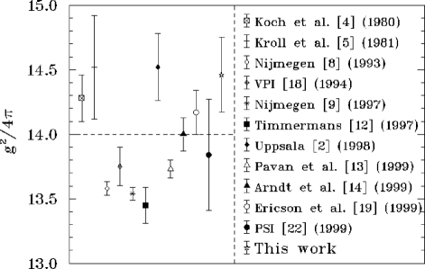
A more direct determination is the use of the Goldberger-Miyazawa-Oehme (GMO) sum-rule [17] which, in principle, depends directly on physical observables. This was applied in particular in Ref. [18] giving a value of $g^{2}_{\pi^{\pm}}/4\pi=13.75\pm 0.15$ and very recently in Ref. [19] leading to $g^{2}_{\pi^{\pm}}/4\pi=14.17\pm 0.17$. Another direct method is based on the extrapolation to the pion pole of precise data on single-energy backward differential np cross sections. Both determinations allow a systematic discussion of statistical and systematic uncertainties. The use of the recent backward np Uppsala data at 162 MeV [2, 20] and of a novel extrapolation method, the difference method, gives $g^{2}_{\pi^{\pm}}/4\pi=14.52\pm 0.26$ [2, 21]. Fairly new analysis of the recent PSI backward np data, with the classical Chew extrapolation and a conformal mapping method leads to $g^{2}_{\pi^{\pm}}/4\pi=13.84\pm 0.43$ [22]. A summary of values for the coupling constant is given in Table 1. It can be seen that between the smallest and largest value there is a discrepancy of about 7%. The dispersion of the different $g^{2}_{\pi^{\pm}}/4\pi$ values can also be judged from Fig. 1.

Figure 1: Some $\pi NN$ coupling constants as found over the last 20 years

Let us recall that, when using the np backward data, the experimental normalisation of the cross section is very important to the sensitivity. It is both the shape of the angular distribution at the most backward angles, and the absolute normalisation of the data, that are of crucial importance [2, 20, 21, 23]. The Nijmegen group has strongly criticised the Uppsala data at 162 MeV and its extrapolated result via the difference method [9, 24]. In particular in Ref. [9] it is claimed that there is a very strong model dependence of the difference method. It is the purpose of the present study to check the accuracy of the difference method and in particular, when applied to the precise 162 MeV Uppsala data we shall demonstrate, by choosing different models, that the model dependence is small and that for good reference models this method leads to a precision smaller than 2%.

The evidence that the backward peak of the np angular distribution is dominated by the one-pion exchange will be discussed in Sect. 2. The determination of the $\pi N\!N$ coupling constant through the extrapolation to the pion pole from models and np data is studied in Sect. 3, and some conclusions are given in Sect. 4.

2 Evidence for the one-pion exchange

Figure 2: Coulomb-like behaviour of the Svedberg Laboratory np CEX data at 162 MeV [2, 20] and prediction of the ’DA99’ model and of other reference models considered here [30].

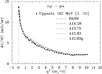
It was early realized that the one-pion exchange (OPE) contributes importantly to the np charge exchange (CEX) at small momentum transfer. In Fig. 2 we have plotted the recent np CEX experimental differential cross section data measured at the Svedberg Laboratory at 162 MeV [2, 20] as a function of $q^{2}$, square of the momentum transfer of the neutron to the proton. It can be seen that there is a strong peak at very small $q^{2}$. Note that in Fig. 2 $q^{2}$ is expressed in units of m_π, the charged pion mass. This differential cross section has a ”Coulomb like behaviour”, it goes to $\infty$, not at $q^{2}=0$ as in the photon-exchange case, but at $q^{2}=-m^{2}_{\pi}$, which corresponds to the pion pole of the OPE. The presence of this OPE pole very close to the physical region led Chew in 1958 to suggest a model-independent extrapolation to this pole which would allow to determine the $\pi N\!N$ coupling constant [25, 26]. We here refer, for the interested reader, to the very detailed and well documented discussion concerning the OPE given in Ref. [2]. We shall now recall the different methods of extrapolation which were considered in that same reference.

3 Extrapolation to the pion pole

Figure 3: Extrapolations to the pion pole at 162 MeV of the Chew function $y(q^{2})$ of the model DA99 [30] for $n$-term polynomial fits and for the reduced range $0<q^{2}<4\ m_{\pi}^{2}$ of the 162 MeV np CEX Uppsala data. Here the errors of these experimental data have been assigned to the model DA99.

3.1 Methods of extrapolation

The idea to extrapolate to the pion pole is to study a smooth physical function, the Chew function, built by multiplying the cross section by $(q^{2}+m_{\pi}^{2})^{2}$. This removes the pole term and the extrapolation can be made more safely and controllably. This function can be then fitted to the data in the physical region by a polynomial and extrapolated to the pole. One considers,

$$y(x)=\frac{(4\pi)^{2}sx^{2}}{m_{\pi}^{4}g_{R}^{4}}\frac{{\rm d}\sigma}{{\rm d}\Omega}(x)=\sum_{{\rm i=0}}^{{\rm n-1}}a_{i}x^{i}.$$ (1)

Here $x=q^{2}+m_{\pi}^{2}$ and $s$ is the square of the total energy. At the pion pole $x=0$ and

$$y(0)\equiv a_{0}\equiv g^{4}_{\pi^{\pm}}/g_{R}^{4}$$ (2)

where the pseudoscalar coupling constant $g^{2}_{\pi^{\pm}}/4\pi\simeq 14$. The quantity $g_{R}^{2}$ is a reference scale for the coupling chosen for convenience. The model-independent extrapolation requires accurate data with absolute normalisation of the differential cross section. If the experimental differential cross section is incorrectly normalised by a factor $N$, the extrapolation determines $\sqrt{N}g^{2}_{\pi^{\pm}}/4\pi$. This is one of the most important sources of uncertainty when extrapolating the data. The Chew method which has been the most used in the past requires at least 5 terms in the $q^{2}$ expansion [2].

Figure 4: 5 terms Ashmore fit of the 162 MeV pseudo-data ‘DA99’ [30] in the full range $0<q^{2}<10.1\ m_{\pi}^{2}$ of the np CEX Uppsala data.

A second method, which should improve the convergence of the Chew extrapolation, is the Ashmore method [27]. It parameterises ${\rm d}\sigma/{\rm d}\Omega(x)$ in terms of a pion Born amplitude with the addition of a background term. Here we use the regularised pion Born amplitudes as given in Ref. [28]. One expects also an important contribution to the np CEX from the $\rho$-meson exchange. We then use for the Ashmore background amplitude a pole term with adjustable strength simulating this $\rho$-meson exchange. This expression is fitted to the data and gives in principle a model-independent result for the coupling constant. More physics is built into the procedure, so fewer terms should be needed. More detailed expressions can be found in Ref [2].

In order to obtain an improvement in the extrapolation we have introduced the Difference Method [21]. It is based on the Chew function, but it uses the fact that an important part of the cross section behaviour is described by models with exactly known values for the coupling constant. It applies the Chew method to the difference between the function $y(x)$ of a model and that of the experimental data, i.e.,

$$y_{Model}(x)-y_{Exp}(x)=\sum_{{\rm i=0}}^{{\rm n-1}}d_{i}x^{i}.$$ (3)

If $g_{R}$ of Eq. (1) is replaced by the model value $g_{Model}$, one has at the pion pole,

$$y_{Model}(0)-y_{Exp}(0)\equiv d_{0}\equiv\frac{g_{Model}^{4}-g^{4}_{\pi^{\pm}}}{g_{Model}^{4}}.$$ (4)

This should decrease systematic extrapolation uncertainties and remove a substantial part of the non-OPE information at large momentum transfers. We have formally not introduced a model dependence by using such a comparison function and such procedures are used in many contexts of physics to obtain better transparency and precision. One has to calibrate the method, that is, to find the precision to which the coupling constant can be determined and the possible systematic uncertainties that are associated with the extrapolation procedure.

3.2 Application to models

Table 2: Coupling constants obtained from $n$-term polynomial fits to the 31 points of several ‘pseudo-data’ models at 162 MeV for the reduced range $0<q^{2}<4\ m_{\pi}^{2}$ with the three extrapolation methods. These models are $NN$ energy dependent PWA’s of R. A. Arndt [30]. The unknown coupling constant of the model ‘DA99’ is to be determined while the reference models A13.75 and A12.83g have $g^{2}_{\pi^{\pm}}/4\pi$ of 13.75 and 12.83 respectively. The column $\delta g^{2}_{\pi^{\pm}}$ is the systematic shift from the true model value. In boldface the value at $\chi^{2}/N_{df}$ = 1.00, retained for the determination of $g^{2}_{\pi^{\pm}}/4\pi$.

n	$\chi^{2}/N_{df}$	$g^{2}_{\pi^{\pm}}/4\pi$	$\chi^{2}/N_{df}$	$g^{2}_{\pi^{\pm}}/4\pi$	$\delta g^{2}_{\pi^{\pm}}$	$\chi^{2}/N_{df}$	$g^{2}_{\pi^{\pm}}/4\pi$	$\delta g^{2}_{\pi^{\pm}}$
	‘DA99’		‘A12.83g’			‘A13.75’
Chew Method
4	1.18	$11.76\pm 0.38$	1.13	$10.40\pm 0.43$	2.43	1.16	$11.27\pm 0.40$	2.48
5	1.00	$13.56\pm 0.84$	1.00	$12.12\pm 0.94$	0.71	1.00	$13.04\pm 0.87$	0.71
Ashmore Method
4	1.01	$13.46\pm 0.47$	1.01	$12.00\pm 0.54$	0.83	1.01	$13.01\pm 0.50$	0.74
5	1.00	$13.89\pm 0.94$	1.00	$12.48\pm 1.11$	0.35	1.00	$13.40\pm 1.03$	0.35
Difference Method
	A12.83g $-$ ‘DA99’		A13.75 $-$ ‘DA99’			A13.75 $-$ ‘A12.83g’
2	3.32	$12.15\pm 0.06$	1.34	$13.51\pm 0.06$		1.88	$14.15\pm 0.05$	1.32
3	1.30	$13.09\pm 0.13$	1.04	$13.85\pm 0.12$		1.12	$13.62\pm 0.13$	0.79
4	1.00	13.97 $\pm$ 0.32	1.00	14.16 $\pm$ 0.32		1.00	$13.05\pm 0.34$	0.22

We now want to cross-check to which precision can work the difference method in the extrapolation to the pion pole. We shall first apply it to models where the coupling is exactly known. This allows to investigate its properties and in particular its systematics. In order to determine the systematic uncertainties in the procedures we have generated pseudo-data with uncertainties corresponding to the Uppsala 162 MeV experiment from 10000 computer simulations using exact data points from different models with a Gaussian, random error distribution [29]. One has for a given pseudo-measurement m,

$$y^{Pseudo-data}_{m}(x)=y^{Model}(x)+\Delta y_{m}(x)$$ (5)

with

$$\Delta y_{m}(x)=\Delta y^{Uppsala}(x)\sqrt{-2Log(R_{1m})}cos(\pi R_{2m}).$$ (6)

In Eq. 6 $R_{im}$, for i=1, 2, are random numbers between 0 and 1 when m varies from 1 to 10000.

In the context of the workshop we have asked R. A. Arndt to provide us with different models from his $NN$ energy dependent PWA. One of the models, which we call A13.75, corresponds to the energy-dependent PWA of the $pp$ and np data from 0 to 400 MeV [30] with a minimisation on $g^{2}_{\pi^{\pm}}/4\pi$ [14]. The minimum $\chi^{2}$ on the $NN$ data is obtained for a coupling constant of 13.75. The second model we consider is built from the previous one with all parameters kept fixed, except the value of the $\pi NN$ coupling constant which is lowered down from 13.75 to 12.83, let us denote this model as A12.83g. A third model, denoted DA99, was also given to us but with an unknown coupling constant. We shall here apply the three methods described in section 3.1 in order to attempt to determine this coupling constant, considering the predictions of this model as pseudo-data. The differential cross section at 162 MeV of the model DA99 is compared to that of the Uppsala experiment in Fig. 2.

Table 3: Same as for Table 2 but for the 54 ‘pseudo-data’ of the full range $0<q^{2}<10.1\ m_{\pi}^{2}$.

n	$\chi^{2}/N_{df}$	$g^{2}_{\pi^{\pm}}/4\pi$	$\chi^{2}/N_{df}$	$g^{2}_{\pi^{\pm}}/4\pi$	$\delta g^{2}_{\pi^{\pm}}$	$\chi^{2}/N_{df}$	$g^{2}_{\pi^{\pm}}/4\pi$	$\delta g^{2}_{\pi^{\pm}}$
	‘DA99’		‘A12.83g’			‘A13.75’
Chew Method
5	1.13	$12.18\pm 0.29$	1.11	$10.74\pm 0.33$	2.09	1.12	$11.65\pm 0.30$	2.10
6	1.02	$13.23\pm 0.51$	1.01	$11.80\pm 0.57$	1.03	1.02	$12.71\pm 0.53$	1.04
7	1.00	$13.86\pm 0.87$	1.00	$12.42\pm 0.97$	0.41	1.00	$13.34\pm 0.90$	0.41
Ashmore Method
4	3.38	$11.96\pm 0.33$	4.13	$\ 9.62\pm 0.41$	3.21	3.65	$11.13\pm 0.35$	2.62
5	1.05	$14.25\pm 0.33$	1.03	$12.64\pm 0.90$	0.19	1.04	$13.69\pm 0.35$	0.06
6	1.03	$13.82\pm 0.78$	1.02	$12.03\pm 0.38$	0.80	1.02	$12.91\pm 0.84$	0.84
Difference Method
	A12.83g $-$ ‘DA99’		A13.75 $-$ ‘DA99’			A13.75 $-$ ‘A12.83g’
3	2.68	$12.23\pm 0.09$	1.24	$13.55\pm 0.08$		1.65	$14.14\pm 0.08$	1.28
4	1.26	$13.31\pm 0.15$	1.04	$13.93\pm 0.14$		1.10	$13.48\pm 0.15$	0.65
5	1.00	14.07 $\pm$ 0.25	1.00	14.20 $\pm$ 0.25		1.00	$12.99\pm 0.27$	0.16

Results are listed in Tables 2 and 3, $n$ being the number of terms in the polynomial fit of the ’pseudo-data’. As for each calculation we performed 10000 pseudo-experiments, $\chi^{2}/N_{df}$ is the average $\chi^{2}$ per degrees of freedom, $g^{2}_{\pi^{\pm}}/4\pi$ is the mean value of the coupling constant and the errors quoted are the standard deviations which, in fact, are very close to the average value of the error of every pseudo-experiment. We also give, for the models A12.83g and A13.75, the systematic deviation $\delta g^{2}_{\pi^{\pm}}$ of the mean value from the true value in the model. We have then a control on systematic extrapolation errors and can calibrate the corresponding corrections. The data is grouped in two intervals, the first one with $0<q^{2}<4\ m_{\pi}^{2}$ called ’reduced range’ with 31 data points, corresponding to the previous Uppsala experiment [21] and the second one with $0<q^{2}<10.1\ m_{\pi}^{2}$ denoted ’full range’ with 54 data points corresponding to the latest experiment [2, 20]. This allows to examine the sensitivity and stability of the extrapolation to a given cut in momentum transfer and to check that it is the small $q^{2}$ region that carries an important part of the pion pole information. As a function of $n$ the behaviour of $\chi^{2}/N_{df}$ is characteristic: it drops quickly with increasing $n$ to a value close to unity. Additional terms give only small benefits, and the data become over-parameterised. One can then adopt different statistical strategies leading to similar results. One is to take results at the minimum $\chi^{2}/N_{df}$. This minimum is usually a shallow one, and values of $n$ close to $n$ of $\chi^{2}/N_{df}$ minimum are almost equally probable statistically. Another possibility is to pick up $g^{2}_{\pi^{\pm}}/4\pi$ from one of the smallest values of $n$ consistent with a $\chi^{2}/N_{df}$ well within the range expected from the experimental sample. We recall the reader that here there is about 47% probability of the experimental $\chi^{2}/N_{df}$ to be larger than unity, and about 25% for it to be larger than 1.15.

Figure 5: Extrapolations of the Chew function $y(q^{2})$ to the pion pole at 162 MeV with the Difference Method on the model DA99 [30] for $n$-term polynomial fits and for the reduced, a), $0<q^{2}<4\ m_{\pi}^{2}$ and full, b), $0<q^{2}<10.1\ m_{\pi}^{2}$ ranges. The reference function is the PWA A12.83g [30]. Here exact prediction of the model is used, the error at each point being that of the corresponding 162 MeV Uppsala data point  [2, 20].

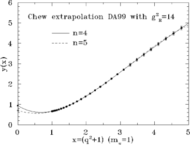
For the Chew method a good fit is performed with a fourth order polynomial in $q^{2}$ for the reduced range, but with a large systematic downward shift of 0.71 for both ’A12.83g’ and ’A13.75’ PWA’s as compared to the original model values. With a third order polynomial fit the statistical error becomes smaller, but the systematic shift is unreasonably large viz. 2.43 and 2.48 respectively. In the full range , one or two more terms are needed to obtain a good fit. In any case a systematic shift remains even when a perfect fit is obtained, but at the minimum $\chi^{2}$ it is always less than the statistical and extrapolation uncertainty. The ’DA99’ pseudo-data for both ranges give slightly different results for $g^{2}_{\pi^{\pm}}/4\pi$ at minimum $\chi^{2}$, but if one applies the corresponding systematic shift one obtains the same value of 14.27(86).The statistical and extrapolation error is rather large so we do not obtain a precise determination of the coupling constant using this method. Fig. 3 shows the fit of the model DA99 in the reduced range together with its Chew-function (Eq. 1) extrapolations for n=4 (dotted line) and n=5 (solid line). The n=5 fit is better for $q^{2}$ above 2 m${}_{\pi}^{2}$.

Figure 6: As in Fig. 5 but for the reference model ’A13.75’ [30].

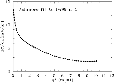
For the Ashmore method a good description is achieved in the reduced range with one term less in the expansion. This shows that the physics beyond the $\pi$-exchange is reasonably described by the $\rho$-exchange, as anticipated in section 3.1. The systematic shifts are similar to those of the Chew method. The statistical and extrapolation error, when one stands close to the minimum $\chi^{2}$, is however smaller. Once corrected by the mean value of the systematic shifts of the models the pseudo-data gives a $g^{2}_{\pi^{\pm}}$ of 14.25(47) with a central value very close to the previous result. In the full range the needed number of terms to get a good $\chi^{2}$ is also smaller and the corrected value for n=5 is 14.37(35). Although the statistical and extrapolation accuracy has improved, this method also appears to lack the high accuracy we would like to have. The excellent fit to the model DA99 is drawn in Fig. 4 for the full range with the Ashmore parameterisation [2] with 5 terms.

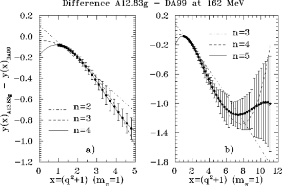
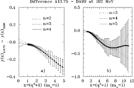
The Difference Method should need less terms in the polynomial expansion than the two above methods, and this will give a smaller, statistical extrapolation error. Recall that the statistical extrapolation errors are only meaningful if $\chi^{2}/N_{df}$ is close to 1. The fact that the angular distributions from the pseudo-data and models might be alike can help, in particular for large $q^{2}$. This can add more physical information without introducing in principle any model dependence. We use the two reference models studied above. Results are given in Tables 2 and 3 for the reduced and full ranges, respectively. The pion-pole extrapolations of the $n$-term polynomial fits of the Difference Method, on the the reduced and full ranges for the model DA99, are shown in Figs. 5 and 6 for the comparison models A12.83g and A13.75, respectively. The error bars increase at large $x$, which is due to the multiplication of the cross section by $x^{2}$, giving a smaller weight for the large $q^{2}$ region when extrapolating. The difference behaviour is slightly smoother with the reference model ’A13.75’, however it can be seen that in all cases 4 and 5 terms are necessary to have a good fit in the reduced and full range, respectively. In the full range, as one has more points, one gets a better statistical extrapolation error, this applies also to the difference between reference models which gives a check on the systematic uncertainties in the extrapolation. Both ranges have systematic shifts below 1%.

Averaging the values at minimum $\chi^{2}$ (values in boldface in Tables 2 and 3) from the Difference-Method extrapolations one gets, over the reduced range,

$$\sqrt{N}g^{2}_{\pi^{\pm}}/4\pi = 14.07\pm 0.32\ (\mbox{statistical + extrapolation})$$

$$\pm 0.11\ (\mbox{systematic})\pm 0.16\ (\mbox{normalisation})$$

$$= 14.07\pm 0.37,$$

i.e. an accuracy of 2.6 %, and over the full range,

$$\sqrt{N}g^{2}_{\pi^{\pm}}/4\pi = 14.14\pm 0.25\ (\mbox{stat. + extr.})\pm 0.08\ (\mbox{syst.})\pm 0.16\ (\mbox{norm.})$$

$$= 14.14\pm 0.31,$$

which corresponds to an accuracy of 2.2 %. The results are fairly close which substantiates our statement on the relevant information being nearly entirely at low $q^{2}$. In view of the somewhat larger extrapolation uncertainty in the case of the reduced range, we take the full range value, 14.14(31), which compares quite well with the exact value of the model DA99 which is 14.28. Using the experimentally given statistics of the 162 MeV Uppsala data, the difference method has allowed us to determine the unknown DA99 coupling to less than 1 % within an uncertainty of 2.2 %.

3.3 Application to data

Table 4: $g^{2}_{\pi^{\pm}}/4\pi$ and $f^{2}_{c}/4\pi$ of the PWA comparison models [30] used here together with their total $\chi^{2}$ and $\chi^{2}$/data on the 3747 np data below 400 MeV.

Model	A12.83g	A12.83	A13.75	A14.28	A14.28g
$g^{2}_{\pi^{\pm}}/4\pi$	12.83	12.83	13.75	14.28	14.28
$f^{2}_{c}/4\pi$	0.071	0.071	0.076	0.079	0.079
$\chi^{2}_{np}(total)$	9282	5087	4975	4958	6149
$\chi^{2}_{np}/data$	2.48	1.36	1.33	1.32	1.64

Figure 7: As in Fig. 5 but for the difference between model A12.83g [30] and Uppsala data [2, 20].

We shall now apply the difference method to the 162 MeV Uppsala data [2, 20] to cross-check the precision of the $g^{2}_{\pi^{\pm}}/4\pi$ determination of Ref. [2]. We here consider different reference models than those used in [2]. Besides the three comparison models considered in the previous section we also use two more PWA fit of the $pp$ and np data from 0 to 400 MeV with $g^{2}_{\pi^{\pm}}/4\pi$ fixed to 12.83 (model A12.83) and 14.28 (model A14.28) [30]. In Table 4 we give the total $\chi^{2}$ and the $\chi^{2}$/data on the 3747 np data considered for all the models we study here. We also recall their $g^{2}_{\pi^{\pm}}/4\pi$ together with the corresponding pseudovector coupling $f^{2}_{c}/4\pi$, related to $g^{2}_{4\pi^{\pm}}/4\pi$ by $g^{2}_{\pi^{\pm}}=f^{2}_{c}(2M_{M_{N}}/m_{\pi^{\pm}})^{2}$ with $M_{N}$ average proton-neutron mass. As for the model A12.83g, the model A14.28g (DA99) was obtained from the model A13.75 with all parameters kept fixed but increasing the $\pi NN$ coupling from 13.75 to 14.28. Predictions of all these comparison models for the 162 MeV Uppsala data are shown in Fig. 2.

Table 5: As in Table 2, but, i) for the difference method only, ii) the 31 points of the pseudo-data of the model DA99 are replaced by those of the 162 MeV Uppsala data [2, 20], iii) with 3 more Arndt PWA reference models [30], viz., A12.83, A14.28 and A14.28g (same as ‘DA99’). Models A12.83 and A14.28 (as also A14.28g) have $g^{2}_{\pi^{\pm}}/4\pi$ of 12.83 and 14.28, respectively. In boldface the experimental values retained for the determination of $g^{2}_{\pi^{\pm}}/4\pi$.

Difference Method
n	$\chi^{2}/N_{df}$	$g^{2}_{\pi^{\pm}}/4\pi$	$\chi^{2}/N_{df}$	$g^{2}_{\pi^{\pm}}/4\pi$	$\delta g^{2}_{\pi^{\pm}}$	$\chi^{2}/N_{df}$	$g^{2}_{\pi^{\pm}}/4\pi$	$\delta g^{2}_{\pi^{\pm}}$
	A12.83g $-$ Uppsala		A12.83 $-$ Uppsala			A13.75 $-$ Uppsala
2	1.60	$13.45\pm 0.05$	1.13	$13.85\pm 0.05$		1.13	$14.69\pm 0.05$
3	1.34	$13.79\pm 0.13$	1.15	$13.75\pm 0.13$		1.06	14.50 $\pm$ 0.12
4	1.03	14.69 $\pm$ 0.31	1.03	14.37 $\pm$ 0.31		1.03	$14.87\pm 0.30$
5	1.07	$14.50\pm 0.79$	1.07	$14.30\pm 0.80$		1.06	$14.54\pm 0.78$
	A14.28 $-$ Uppsala		A14.28g $-$ Uppsala			A13.75 $-$ ‘12.83’
2	1.17	$15.20\pm 0.05$	1.72	$15.42\pm 0.05$		1.05	$13.76\pm 0.05$	0.93
3	1.02	14.96 $\pm$ 0.12	1.00	14.94 $\pm$ 0.12		1.03	$13.65\pm 0.13$	0.82
4	1.04	$15.19\pm 0.30$	1.03	$15.00\pm 0.30$		1.01	$13.40\pm 0.33$	0.57
5	1.06	$14.72\pm 0.77$	1.06	$14.59\pm 0.78$		1.00	$13.09\pm 0.87$	0.26
			A12.83 $-$ ‘A14.28’			A13.75 $-$ ‘A14.28’
2			1.14	$12.86\pm 0.06$	-1.42	1.02	$13.76\pm 0.05$	-0.52
3			1.07	$13.04\pm 0.13$	-1.24	1.01	$13.83\pm 0.12$	-0.45
4			1.01	$13.43\pm 0.33$	-0.85	1.00	$13.96\pm 0.32$	-0.32
5			1.00	$13.83\pm 0.83$	-0.45	1.00	$14.09\pm 0.81$	-0.19

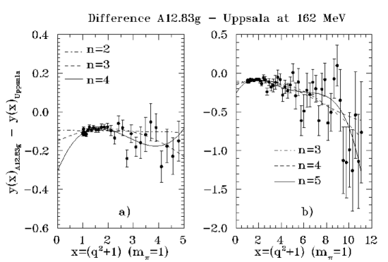
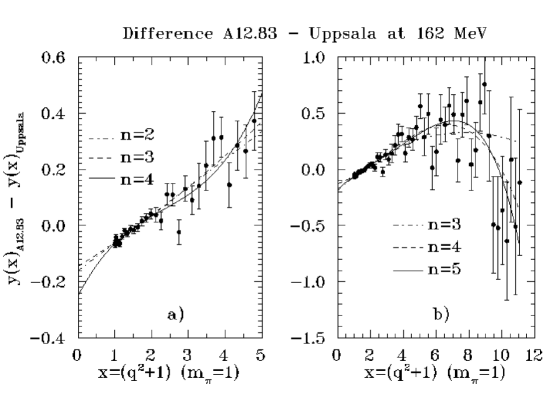
Results for the reduced and full range are listed in Tables 5 and 6 respectively. The A12.83g comparison model requires 4 terms in the reduced range and 5 in the full one. Figure 7 shows that there is some edge effect in the reduced range at $q^{2}=4m^{2}_{\pi}$. For the model A12.83 one needs also 4 terms in the reduced range. The obtained value, 14.37(31) is quite consistent with those determined in the model A12.83g, either in the reduced range, 14.69(31) or in the full range, 14.41(24). In the full range the minimum is very shallow and the $n=4\ (\chi^{2}/N_{df}=1.18)$ and $n=5\ (\chi^{2}/N_{df}=1.16)$ values, 13.65(14) and 13.94(25), respectively, are compatible. The lower value, 13.65(14), is however not compatible with the value, 14.37(31) of the reduced range at $\chi^{2}/N_{df}$ minimum, We shall then retain, in the full range for the A12.83 model, the $n=5$ determination, 13.94(25). Figure 8 shows as before the necessity to have at least 4 or 5 terms to obtain a good fit. In the reduced range 3 terms are here sufficient with the reference model A13.75 leading to $g^{2}_{\pi^{\pm}}/4\pi=14.50(12)$ while in the full range $\chi^{2}$ minimum is reached with 4 terms with a value of 14.38(14). Figure 9 shows in both range a smoother behaviour than before. In the A14.28 and A14.28g case one needs the same number of terms as for A13.75 but the corresponding $g^{2}_{\pi^{\pm}}/4\pi$ are somewhat larger and not always compatible with previous values. Curves for the extrapolation are shown in Figs. 10 and 11. Applying the difference method between models (see also Tables 2 and 3) shows relatively large systematics which allows to understand this dispersion.

Table 6: As in Table 5 but for the 54 Uppsala data points at 162 Mev of the full range $0<q^{2}<10.1\ m_{\pi}^{2}$.

Difference Method
n	$\chi^{2}/N_{df}$	$g^{2}_{\pi^{\pm}}/4\pi$	$\chi^{2}/N_{df}$	$g^{2}_{\pi^{\pm}}/4\pi$	$\delta g^{2}_{\pi^{\pm}}$	$\chi^{2}/N_{df}$	$g^{2}_{\pi^{\pm}}/4\pi$	$\delta g^{2}_{\pi^{\pm}}$
	A12.83g $-$ Uppsala		A12.83 $-$ Uppsala			A13.75 $-$ Uppsala
3	1.30	$13.65\pm 0.08$	1.36	$14.02\pm 0.08$		1.43	$14.84\pm 0.07$
4	1.30	$13.79\pm 0.14$	1.18	$13.65\pm 0.14$		1.12	14.38 $\pm$ 0.14
5	1.14	14.41 $\pm$ 0.24	1.16	13.94 $\pm$ 0.25		1.14	$14.53\pm 0.24$
6	1.15	$14.74\pm 0.46$	1.16	$14.42\pm 0.47$		1.15	$14.80\pm 0.45$
	A14.28 $-$ Uppsala		A14.28g $-$ Uppsala			A13.75 $-$ ‘12.83’
3	1.51	$15.33\pm 0.07$	2.15	$15.53\pm 0.07$		1.03	$13.74\pm 0.08$	0.91
4	1.11	14.83 $\pm$ 0.13	1.12	14.75 $\pm$ 0.13		1.02	$13.63\pm 0.14$	0.80
5	1.13	$14.89\pm 0.24$	1.13	$14.62\pm 0.24$		1.01	$13.49\pm 0.26$	0.66
6	1.15	$15.05\pm 0.45$	1.15	$14.86\pm 0.45$		1.00	$13.27\pm 0.50$	0.44
			A12.83 $-$ ‘A14.28’			A13.75 $-$ ‘A14.28’
3			1.08	$12.89\pm 0.09$	-1.41	1.01	$13.77\pm 0.08$	-0.51
4			1.04	$13.07\pm 0.15$	-1.21	1.01	$13.83\pm 0.14$	-0.45
5			1.02	$13.30\pm 0.26$	-1.13	1.00	$13.92\pm 0.25$	-0.36
6			1.01	$13.62\pm 0.49$	-0.66	1.00	$14.02\pm 0.48$	-0.26

Figure 8: As in Fig. 5 but for the difference between model A12.83 [30] and Uppsala data [2, 20].

Figure 9: As in Fig. 5 but for the difference between model A13.75 [30] and Uppsala data [2, 20].

Figure 10: As in Fig. 5 but for the difference between model A14.28 [30] and Uppsala data [2, 20].

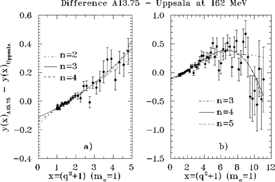
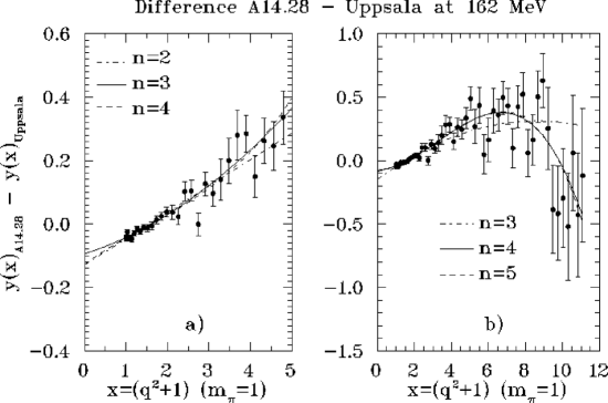
Let us here remind the reader that the difference method analysis is quite consistent. One can check, in the Tables 2, 3, 5 and 6, that, at a given $n$ value, the difference between the results of the difference method for the reference models and data is very close to the systematic shift between the two models. One has,

$$g^{2}_{\pi^{\pm}}/4\pi(n,\ \mbox{Model A}-\mbox{Uppsala}) - g^{2}_{\pi^{\pm}}/4\pi(n,\ \mbox{Model B}-\mbox{Uppsala})$$ (7)

$$\simeq \delta g^{2}_{\pi^{\pm}}(n,\ \mbox{Model A}-\mbox{Model B}).$$

For instance if we compare in the full range the $n=4$, (A13.75 $-$ Uppsala) result to that of (A12.83g $-$ Uppsala) we have a difference (see Table 6) of 0.59 (14.38 - 13.79) which is close to the systematic shift between these models .65 (see Table 3 ). In Ref. [2] where the comparison models were the Nijmegen potential [31], the Nijmegen [32] (NI93) and Virginia [33, 34] (SM95) energy dependent PWA’s, dispersion of results were smaller. This could be traced to the fact that these models, where $g^{2}_{\pi^{\pm}}/4\pi$ has been minimised with respect to the $NN$ data, have a high $q^{2}$ momentum more similar to that of the Uppsala data.

Figure 11: As in Fig. 5 but for the difference between model A14.28g [30] and Uppsala data [2, 20].

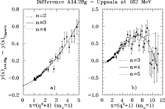
Summarising these results we take for $g^{2}$ the following average in the reduced range

$$g^{2}_{\pi^{\pm}}/4\pi = \frac{1}{5}[14.69(31)+14.37(31)+14.50(12)+14.96(12)+14.94(12)]$$ (8)

$$= 14.69(20)$$

It is here only the second value (from A12.83$-$Uppsala) which is slightly outside the range of the 2 last values from A14.28 and A14.28g

Taking half of the average of $|\delta g^{2}_{\pi^{\pm}}|$ between models at $\chi^{2}/N_{df}=1.00$ for the estimation of the systematic uncertainty (see Table 5) we obtain

$$g^{2}_{\pi^{\pm}}/4\pi = 14.69\pm 0.20\ \mbox{(stat. + extr.)}\pm 0.15\ \mbox{(syst.)}\pm 0.17\ \mbox{(norm.)}$$ (9)

$$= 14.69(30)$$

i.e. an accuracy of 2 %. For the full range (see Table 6) we have

$$g^{2}_{\pi^{\pm}}/4\pi = \frac{1}{5}[14.41(24)+13.94(25)+14.38(14)+14.83(13)+14.75(13)]$$ (10)

$$= 14.46(18)$$

Adding the systematic (estimated as above) and normalisation errors we obtain

$$g^{2}_{\pi^{\pm}}/4\pi = 14.46\pm 0.18\ \mbox{(stat.+ extr.)}\pm 0.15\ \mbox{(syst.)}\pm 0.17\ \mbox{(norm.)}$$ (11)

$$= 14.46(29)$$

i.e. again an accuracy of 2%. Note that for A12.83 $-$ A14.28 we need to go to $n=7$ to get $\chi^{2}/N_{df}=1.00$ with a $\delta g^{2}_{\pi^{\pm}}$ of $-$0.36. The value of Eq. (11) is to be compared to the value we determined in Ref. [2], viz.

$$g^{2}_{\pi^{\pm}}/4\pi = 14.52\pm 0.13\ \mbox{(stat.+ extr.)}\pm 0.15\ \mbox{(syst.)}\pm 0.17\ \mbox{(norm.)}$$ (12)

$$= 14.52(26)$$

i.e. an accuracy of 1.8%. It is seen that both determination, Eqs. (11) and (12), are very close. The determination of Ref. [2], Eq. (12) has a better statistical extrapolation error which can be understood as the comparison model have possibly a better determined high $q^{2}$ behaviour as just mentioned above.

4 Conclusions

This analysis of the 162 Mev Uppsala precise experiment on np charge exchange demonstrates here again that such data can be used for a direct and accurate determination of the $\pi N\!N$ coupling constant. We reproduce the original coupling constant using the present procedures for pseudo-data from PWA’s as exemplified with the model DA99. The extrapolation error increases with the number of parameters. Our value is 7% larger than the Nijmegen [8] result $g^{2}_{\pi^{\pm}}=13.58\pm 0.05$, but it is consistent with values given in earlier data compilations based on the analysis of $\pi N$ and $N\!N$ scattering data [35].

The data have been used to determine a precise value for the charged $\pi N\!N$ coupling constant using extrapolation to the pion pole. Using the most accurate extrapolation method, the Difference Method, we find $\sqrt{N}g^{2}_{\pi^{\pm}}=14.46\pm 0.18$ ($f^{2}_{\pi^{\pm}}=0.0800\pm 0.001$) with a systematic error of about $\pm 0.15$ ($\pm 0.0008$) and a normalisation uncertainty of $\pm 0.17$ ($\pm 0.0009$). We do reproduce the input coupling constants of models using equivalent pseudo-data. The practical usefulness of the method, its precision and its relative insensitivity to systematics appear to be under control. The pseudo-data demonstrate that considerable precision is achieved statistically at a single energy. The absolute normalisation of the data is nevertheless crucial. The precision of the method used here has not yet reached its theoretical limit, but we can point out the key information necessary for this in the $N\!N$ sector. We need as precise as possible unpolarised differential cross sections with an absolute normalisation of 1 to 2% to reach a precision of about 1% in the coupling constant. For the Uppsala data an accurate normalisation [2, 20] of 2.3 % was obtained using integration over the angular distribution. It was performed on the part they measured (from 72^∘ to 180^∘) and on the remaining one calculated from PWA’s and models. The result was scaled to the well known experimentally total cross section [36]. It is important to extend the angular range of data, to be able to achieve an improved normalisation.

For that purpose there is, as we have heard [20] in this workshop, an experiment in progress at The Svedberg Laboratory. It will measure the np differential cross section in the forward hemisphere. This should hopefully determine the normalisation to 1 % and then lower down the accuracy on $g^{2}_{\pi^{\pm}}/4\pi$ from 1.8 % to 1.5 %. To the question which was asked at this workshop “Does the difference method work at the 1 % level?” the answer is so far no, but as we have demonstrate it can work to less than 2 %, in particular with good reference models we obtained a precision of 1.8 %. Here with different reference models the precision reached was 2 %. Contrary to what was claimed in Ref. [9] we do not see a large model dependence, even using “extreme” models as the A12.83g with $g^{2}_{\pi^{\pm}}/4\pi$=12.83 or $f^{2}_{c}/4\pi$=0.071. The model dependence is relatively small as can be judged from a comparison of the result here and that of Ref. [2] where while using different reference models the results agree within less than 0.5 %.

Let us also mention, as we were told [37] in this workshop that np backward measurement with tagged neutron beams (which leads to absolute normalisation) are in progress at IUCF for 185 $\geq T_{lab}\leq$ 195 MeV and $90^{\circ}<\theta<180^{\circ}$. If the very backward steeper shape of the Uppsala data as compared with earlier data [2, 20, 23] is confirmed together with its absolute normalisation then the $\pi NN$ coupling constant cannot be as low as found, for instance, by the Nijmegen group. If the Uppsala data is correct and if the coupling constant is small then to reconciliate both, either the total cross section could be off or the angular distribution in the forward hemisphere could be different of what it is believed so far from PWA analyses. Hopefully the two above mentioned experiments in progress should help to clarify the situation. There will be also pp and np spin-transfer measurements which could be used to precise the $\pi NN$ coupling constant [38].

In principle, an experiment at one single energy is enough to determine $g^{2}_{\pi^{\pm}}/4\pi$, for all energies contain similar information. Although the method of analysis seems to work well, it is, however, useful to deduce the coupling constant from data at several energies. This would increase confidence that some unexpected systematic effect influences the conclusion.

We thank the The Svedberg Laboratory crew for the data. We are also grateful to J. Blomgren, M. Lacombe and N. Olsson for helpful discussions and to W.R. Gibbs for advice on producing pseudo-data from models. TE acknowledges an interesting discussion with M. Rentmeester and BL the hospitality of the The Svedberg Laboratory.

This work has been financially supported by the Swedish Natural Science Research Council and, grâce au Service Scientifique et Technique de l’Ambassade de France à Stockholm en Suède, par le Ministère des Affaires Étrangères Français.

References

- [1] M.L. Goldberger and S.B. Treiman, Phys. Rev. 110, 1178 (1958).
- [2] J. Rahm, J. Blomgren, H. Condé, S. Dangtip, K. Elmgren, N. Olsson, T. Rönnqvist, R. Zorro, A. Ringbom, G. Tibell, O. Jonsson, L. Nilsson, P.-U. Renberg, T.E.O. Ericson and B. Loiseau, Phys. Rev. C57, 1077 (1998).
- [3] J. L. Goity, R. Lewis, M. Schwellinger L. and Zhang, Phys. Lett. B 454, 115 (1999).
- [4] R. Koch and E. Pietarinen, Nucl. Phys. A336, 331 (1980).
- [5] P. Kroll, Physics Data 22-1, ed. H. Behrens and G. Ebel (Fachinformationszentrum, Karlsruhe, 1981).
- [6] J. R. Bergervoet, P. C. van Campen, R. A. M. Klomp, J.-L. de Kok, T. A. Rijken, V. G. J. Stoks, and J. J. de Swart, Phys. Rev. C 41, 1435 (1990).
- [7] R. A. M. Klomp, V.G.J. Stoks, and J. J. de Swart, Phys. Rev. C 44, R1258 (1991).
- [8] V. Stoks, R. Timmermans, and J. J. de Swart, Phys. Rev. C 47, 512 (1993).
- [9] J. J. de Swart, M. C. M. Rentmeester and R. G. E. Timmermans, N Newsletter 13 (1997) 96.
- [10] R. A. Arndt, Z. Li, D. Roper, and R. L. Workman, Phys. Rev. Lett. 65, 157 (1990).
- [11] R. A. Arndt, I. I. Strakovsky, and R. L. Workman, Phys. Rev. C 50, 2731 (1994).
- [12] R. G. E. Timmermans, N Newsletter 13, 80 (1997).
- [13] M. Pavan et al., N partial wave analysis and the coupling constant, contribution to this workshop.
- [14] R. Arndt et al., Which data are determining the value of the coupling constant in partial-wave analyses?, contribution to this workshop.
- [15] T. Meissner and E.M. Henley, Phys. Rev. C 55, 3093 (1997).
- [16] R. Machleidt, How sensitive are various NN observables to changes in the coupling constant?, contribution to this workshop.
- [17] M. L. Goldberger, H. Miyazawa and R. Oehme, Phys. Rev. 99 (1955) 986.
- [18] R.A. Arndt, R.L. Workman, and M.M. Pavan, Phys. Rev. C 49, 2729 (1994).
- [19] T. E. O. Ericson, B. Loiseau, and A. W. Thomas, The GMO sumrule and the coupling constant, contribution to this workshop.
- [20] N. Olsson et al., Uppsala neutron-proton scattering experiments and the coupling constant, contribution to this workshop.
- [21] T.E.O. Ericson, B. Loiseau, J. Nilsson, N. Olsson, J. Blomgren, H. Condé, K. Elmgren, O. Jonsson, L. Nilsson, P.-U. Renberg, A. Ringbom, T. Rönnqvist, G. Tibell, and R. Zorro, Phys. Rev. Lett. 75, 1046 (1995).
- [22] H.Schmitt et al., The PSI data and their effect on the coupling constant, contribution to this workshop; J. Franz, V. Grundies, A. Habib, W. Hürster, G. Nicklas, E. Rössle, G. Rupp, H. Schmitt, L. Schmitt, and H. Woolverton, to be published.
- [23] J. Blomgren et al., Implications of the inconsistencies in the neutron-proton data, contribution to this workshop.
- [24] Comment by M. C. M. Rentmeester et al., Phys. Rev. Lett. 81 (1998) 5253; Reply by T. E. O. Ericson et al., Phys. Rev. Lett. 81 (1998) 5254.
- [25] G.F. Chew, Phys. Rev. 112, 1380 (1958).
- [26] P. Cziffra and M.J. Moravcsik, Phys. Rev. 116, 226 (1959).
- [27] A. Ashmore, W.H. Range, R.T. Taylor, B.M. Townes, L. Castillejo and R.F. Peierls, Nucl. Phys. 36, 258 (1962).
- [28] W.R. Gibbs and B. Loiseau, Phys. Rev. C 50, 2742 (1994)
- [29] See, e.g., William R. Gibbs, Computation in Modern Physics (World Scientific, Singapore, 1994), p. 35.
- [30] R. A. Arndt (private communication).
- [31] V.G.J. Stoks, R.A.M. Klomp, C.P.F. Terheggen, and J.J. de Swart, Phys. Rev. C 49, 2950 (1994). Data as given by SAID, Ref. [33].
- [32] V.G.J. Stoks, R.A.M. Klomp, M.C.M. Rentmeester, and J.J. de Swart, Phys. Rev. C 48, 792 (1993). Data as given by SAID, Ref. [33].
- [33] Scattering Analysis Interactive Dial-Up (SAID), Virginia Polytechnic Institute, Blackburg, VA, USA (R.A. Arndt, private communication).
- [34] R.A. Arndt, I.I. Strakovsky, R.L. Workman, Phys. Rev. C 52, 2246 (1995).
- [35] O. Dumbrajs, R. Koch, H. Pilkuhn, G.C. Oades, H. Behrens, J.J. de Swart, and P. Kroll, Nucl. Phys. B216, 277 (1983).
- [36] P.W. Lisowski, R.E. Shamu, G.F. Auchampaugh, N.S.P. King, M.S. Moore, G.L. Morgan, and T.S. Singleton, Phys. Rev. Lett. 49, 255 (1982); V. Grundies, J. Franz, E. Rössle, and H. Schmitt, Phys. Lett. B158, 15 (1985).
- [37] T. Peterson, Impact on the coupling constant of the IUCF measurement with a tagged neutron beam, contribution to this Workshop.
- [38] S. Wissink, Implications for the coupling constant from pp and np spin transfer measurements, contribution to this Workshop.