1. INTRODUCTION

Many problems in theoretical physics can be reduced to a calculation of functional integrals of the type

$$I=\int D\varphi\exp(-S_{0}\{\varphi\}-gS_{\rm int}\{\varphi\}),$$

whose expansion in the coupling constant $g$ gives an ordinary perturbation theory. In 1977 Lipatov [1] proposed a method for calculating the high-order expansion coefficients of the integrals (1) on the basis of the following simple idea. If the function $F(g)$ is expanded into a series

$$F(g)=\sum\limits_{N=0}^{\infty}F_{N}g^{N},$$

the $N$th expansion coefficient can be calculated from the formula

$$F_{N}=\oint\limits_{C}\frac{dg}{2\pi i}\frac{F(g)}{g^{N+1}},$$

where the contour $C$ encloses the point $g=0$ in the complex plane. Taking the integral (1) as $F(g)$, we obtain

$$I_{N-1}=\frac{1}{2\pi i}\int dg\int D\varphi\exp(-S_{0}\{\varphi\}-gS_{\rm int}\{\varphi\}-N\ln g),$$

and the appearance of an exponential with a large exponent indicates that the saddle-point method can be applicable at large $N$. Lipatov’s idea is to seek the saddle point in (3) with respect to $g$ and $\varphi$ simultaneously: such saddle-point exists for all the cases of interest and is realized on a spatially localized function, which has been termed an instanton. Moreover, the conditions for applicability of the saddle-point method are satisfied at large $N$.

The Lipatov technique, which was originally applied to scalar theories, such as $\varphi^{4}$ theory

$$S_{0}\{\varphi\}+gS_{\rm int}\{\varphi\}=\int d^{d}x\left\{\frac{1}{2}(\nabla\varphi)^{2}+\frac{1}{2}m^{2}\varphi^{2}+\frac{1}{4}g\varphi^{4}\right\},$$

was subsequently generalized to vector fields [2], scalar electrodynamics [3, 4], Yang–Mills fields [5], fermion fields [6], etc. (see the collection of articles in Ref. [7]). The ultimate goal was to apply it to theories of practical interest, viz., quantum electrodynamics [8, 9] and quantum chromodynamics (QCD) [10, 11]. As was pointed out already in Lipatov’s first paper [1], the knowledge of the first few coefficients and their asymptotic behavior permits approximate reconstruction of the Gell-Mann–Low function, opening up a direct route to the solutions of the problem of confinement and electrodynamics at short distances.

However, a conception which raised some doubts regarding the Lipatov technique was conceived already in 1977. It was initiated by a paper by Lautrup [12], which contained the following curious observation. The typical result of calculations based on the Lipatov technique has a functional form

$$I_{N}=ca^{N}\Gamma(N+b)\approx ca^{N}N^{b-1}N!$$

and the natural interpretation of it is that there is a factorially large number of diagrams of the same order $(ag)^{N}$. However, in the general case such an interpretation is incorrect, since there are examples of individual $N$th-order diagrams having a value ${\sim}N!$. The latter are diagrams (Fig. 1) which contain long chains of “bubbles”.

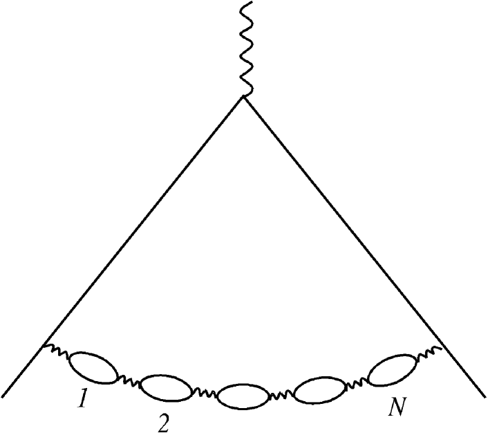
Figure 1:   Example of a diagram for quantum electrodynamics, which makes a contribution ${\sim}N!$ to the $N$th order of perturbation theory [12].

Such factorial contributions of individual diagrams were termed renormalons, since they appear only in renormalizable theories.  Lautrup’s example (Fig. 1) was related to quantum electrodynamics, but similar diagrams exist in QCD and four-dimensional $\varphi^{4}$ theory.

Strictly speaking, nothing followed from Lautrup’s observation: the Lipatov technique is based on a formal calculation of the functional integral (3) and does not rely in any way on a statistical analysis of diagrams. It is natural to expect that the renormalon contributions have already been taken into account in the instanton result (5). In fact, no far-reaching claims were made in Ref. [12] or in the relevant publications appearing shortly thereafter [13, 14].

However, the tone of the publications subsequently changed dramatically. The reason was ’t Hooft’s lecture [15], which was delivered in the same year, 1977. The term ”renormalon” was used in it for the first time, and it was asserted that renormalons are not contained in the instanton contribution (5). The authors of the subsequent publications [16]–[30] considered ’t Hooft’s opinion to be self-evident and did not trouble themselves with argumentation.

A convenient language for discussion, viz., the analytic properties of Borel transforms, was introduced in ’t Hooft’s lecture. The Borel transformation

$$F(g)=\sum\limits_{N=0}^{\infty}F_{N}g^{N}=\sum\limits_{N=0}^{\infty}\frac{F_{N}}{N!}\int\limits_{0}^{\infty}dx\,x^{N}e^{-x}g=\int\limits_{0}^{\infty}dx\,e^{-x}\sum\limits_{N=0}^{\infty}\frac{F_{N}}{N!}(gx)^{N},$$

which factorially improves the convergence, is widely used in the theory of divergent series [30]. It is convenient to rewrite it in the form

$$F(g)=\int\limits_{0}^{\infty}dx\,e^{-x}B(gx),$$

$$B(z)=\sum\limits_{N=0}^{\infty}\frac{F_{N}}{N!}z^{N}$$

by introducing the Borel transform $B(z)$ of the function $F(g)$. The Borel transform for a function with the expansion coefficients (5)

$$B_{I}(z)=\sum\limits_{N}ca^{N}N^{b-1}z^{N}\sim(1-az)^{-b},\ \ za\rightarrow 1$$

has a singularity at the point $z=1/a$.

’t Hooft arrived at this result in a different way, without reference to the Lipatov technique. Rewriting the integral (1) and the definition of the Borel transform (6) in the form

$$I=\int D\varphi\exp(-S\{\varphi\}/g),$$

$$F(g)=\int\limits_{0}^{\infty}dx\,e^{-x/g}B(x),$$

which can be accomplished by means of the replacements $\varphi\rightarrow\varphi/\sqrt{g}$ and $x\rightarrow x/g$ in (4) and (6),  yields the Borel transform of the integral (9):

$$B_{I}(z)=\int D\varphi\delta(z-S\{\varphi\})=\oint\limits_{z=S\{\varphi\}}\frac{d\sigma}{|\nabla S\{\varphi\}|},$$

where the latter integration is carried out over the hypersurface $z=S\{\varphi\}$. If an instanton $\varphi_{c}(x)$, i.e., a classical solution with a finite action, exists for the integral (9), then $\delta S\{\varphi_{c}\}=0$ and the partial derivatives $\partial S/\partial\varphi_{i}$ with respect to all the variables $\varphi_{i}$ comprising $D\varphi$ vanish; therefore, $\nabla S\{\varphi_{c}\}=0$ and the Borel transform (11) has a singularity at the point

$$z=S\{\varphi_{c}\},$$

which coincides with $1/a$. In addition, there are singularities at the points $mS\{\varphi_{c}\}$, which correspond to solutions containing $m$ infinitely distant instantons. If it is assumed that the singularity (12) is closest to the origin of coordinates, the result (5) of the Lipatov technique is reproduced. However, ’t Hooft allowed the existence of singularities differing from those of the instanton type: in this case the asymptotics of the expansion coefficients can be specified by the singularity which is closest to the origin of coordinates.

’t Hooft regarded renormalons as a possible mechanism for the appearance of the new singularities. Let us take an arbitrary diagram for quantum electrodynamics and single out the line of a virtual photon with the momentum $k$ (or an interaction line in $\varphi^{4}$ theory) in it (Fig. 2,a): it corresponds to integration

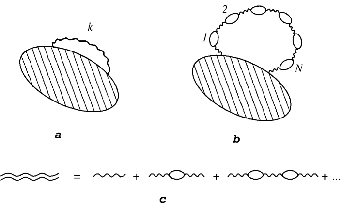
Figure 2:   More general class of renormalon diagrams

over a region of large momenta of the type

$$\int\limits_{k>k_{0}}d^{4}k\,k^{-2m},$$

where $m$ is an integer. If we assume that all the renormalizations have been performed, the integral converges and $m\geq 3$. Inserting a chain of $N$ “bubbles” into the photon line (Fig. 2,b), we obtain the integral  

$$\int\limits_{k>k_{0}}d^{4}k\,k^{-2m}(\beta_{0}\ln k^{2})^{N}\sim\beta_{0}^{N}=\int\limits_{0}^{\infty}dt\,t^{N}e^{-(m-2)t}\sim\left(\frac{\beta_{0}}{m-2}\right)^{N}N!.$$

Borel summation of a sequence of such diagrams gives singularities at the points

$$z=\frac{m-2}{\beta_{0}},\ \ m=3,4,5,\ldots.$$

The constant $\beta_{0}$ is the first nonvanishing expansion coefficient of the Gell-Mann–Low function (Sec. 2), and with consideration of the sign relationships ($S\{\varphi_{c}\}<0$, $\beta_{0}>0$) ’t Hooft arrived at the picture of singularities for $\varphi^{4}$ theory shown in Fig. 3,a.

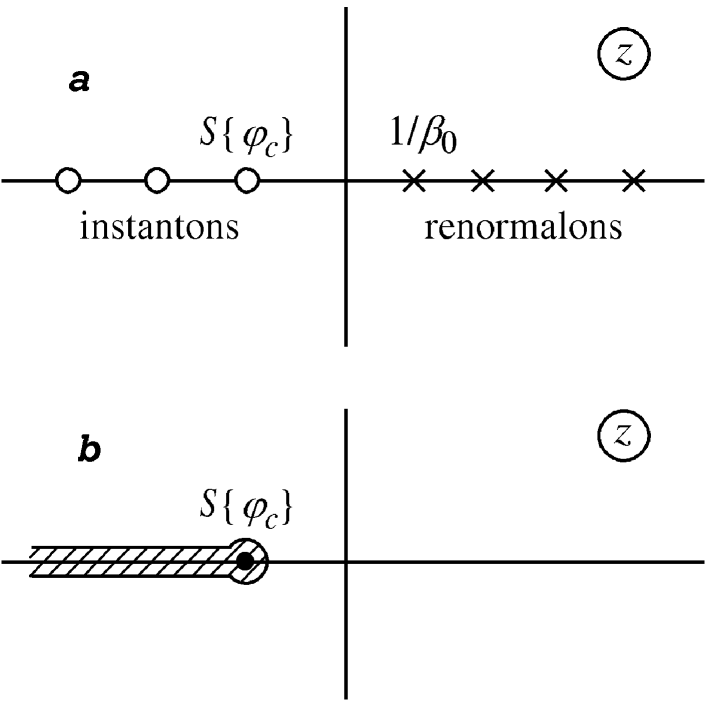
Figure 3:   a) Picture of singularities for $\varphi^{4}$ theory given by ’t Hooft [15].   b) Analyticity region according to the results of the present work.

It is not difficult to see that ’t Hooft’s arguments regarding renormalons leave some fundamental questions unanswered:

Why can significance be attached to individual sequences of diagrams, which make up an infinitesimal fraction of their total number when $N\rightarrow\infty$?

How do we know that the renormalons have not already been taken into account in the instanton contribution (5)?

However, the general setting the question on the possible contributions of a noninstanton nature to the asymptotics of the expansion coefficients has a sense: it uncovers a gap in the mathematical foundation of the Lipatov approach. Indeed, let the function $f(x)$ have a sharp maximum at the point $x_{0}$ and a slow tail at large values of $x$ (Fig. 4,),

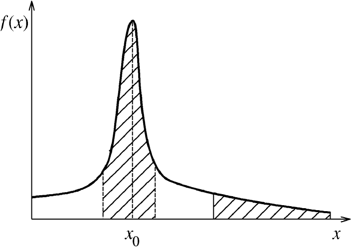
Figure 4:   Example of a function for which the saddle-point method is formally applicable, but gives a wrong result.

so that the contributions to the integral $\int f(x)\,dx$ from the vicinity of the maximum and from the tail region are comparable. An investigation of the integral for a saddle point discloses a maximum at $x_{0}$ and (provided it is sufficiently sharp) the formal applicability of the saddle-point method; however, a calculation of the integral in the saddle-point approximation will be erroneous, since the contribution of the tail will be lost. If such tails are present in the integral (3), the Lipatov technique can be incorrect.  

The essential lack of nonsaddle-point methods for calculating functional integrals makes it impossible to straightforwardly investigate the contribution of possible tails. But are there constructive arguments pointing to their existence? In principle, such arguments exist, but they have a fairly intuitive and ambiguous character and do not hold up to criticism when they are closely examined (Sec. 2). As a result, the conception of renormalons has been in a dialectic equilibrium, i.e., it has not been proved or refuted. This uncertainty has caused the interest in high orders of perturbation theory to drop sharply and Lipatov’s program [1] to remain uncompleted. For example, a preliminary result for quantum electrodynamics was obtained back in 1978 [9], but the parameters $b$ and $c$ in the asymptotics $I_{N}=ca^{N}\Gamma(N/2+b)$ have not yet been calculated. Moreover, the first result for QCD appeared in 1991 (Ref. [10]) and was recently revised [11], but it is still unsatisfactory (Sec. 4), although the foundation for such calculations was completely ready in 1980 [5, 6]. Finally, the attempts to reconstruct the Gell-Mann–Low function have been restricted to $\varphi^{4}$ theory [33, 34, 35].

A reawakening of interest in asymptotic estimates has recently been observed, but it has been confined almost exclusively to the renormalon doctrine [21]–[30]. In particular, it is generally accepted (see Zakharov’s review [21]) that renormalons determine the perturbation asymptotics in QCD. However, the work within the renormalon approach has already raised some doubts: the summation of larger sequences of diagrams leads to dramatic renormalization of the renormalon contribution and renders the common coefficient in front of them totally indefinite [30]; in fact, it is impossible to state that it does not vanish. On the other hand, the use of the Lipatov technique has provided significant progress in the theory of disordered systems [36] and in the theory of turbulence [37].

This paper presents a detailed discussion of the existing arguments in favor of renormalons, which are shown to be unsound (Sec. 2). The analytic properties of Borel transforms are investigated in the example of $\varphi^{4}$ theory (Sec. 3), and their analyticity in a complex plane with a cut from the first instanton singularity to infinity is demonstrated (Fig. 3,b). It rules out the existence of the renormalon singularities indicated by ’t Hooft (Fig. 3,a) and demonstrates the nonconstructiveness of the conception of renormalons as a whole.

An hypothesis that Borel transforms have the analytic properties indicated was advanced by Le Guillou and Zinn-Justin [38] and underlies one of the most efficient methods for summing perturbation series, which is based on the use of conformal transformation. The results obtained below provide the mathematical foundation of this method.

Let us discuss the arguments in the literature that point to the existence of noninstanton contributions in the integral (3).

1.

There have been numerous semi-intuitive assertions which reduce to the notion that instantons do not exhaust all of physics. This thesis is correct as long as it is understood correctly, but in the present case it is not relevant.

Historically, instantons first appeared when the saddle-point approximation was employed in the original integral (1). It was substantiated only in a narrow region of parameters, and thus instantons did not, in fact, exhaust all of physics. In the Lipatov technique the situation changed, because the saddle-point approximation is used not in the integral (1), but in the expression (3) for the expansion coefficients. Since only large values of $N$ are considered, only a limited role is assigned to instantons from the onset; however, the saddle-point method is now always applicable,   and there is a basis to assume that everything is determined by instantons.

Let us illustrate the foregoing statements in the example of the Schrödinger equation with a random potential $V(x)$:

$$[\hat{p}^{2}/2m+V(x)]\Psi(x)=E\Psi(x).$$

At large negative values of $E$ its eigenfunctions (Fig. 5)

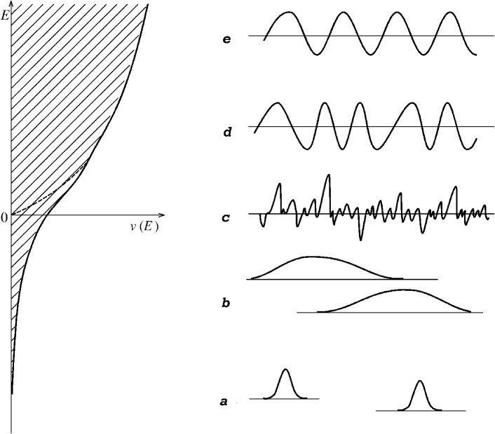
Figure 5:   On the left — density of states $\nu(E)$ in the presence (solid curve) and absence (dashed curve) of a random potential. On the right — schematic representations of the eigenfunctions of Eq. (15).

are localized on the infrequent fluctuations of the random potential (a and b), at large positive values of $E$ they are similar to plane waves (d and e), and in the vicinity of the bare spectrum edge at $E=0$ they have a highly broken, fractal character (c). The problem of investigating Eq. (15) can be reformulated in the language of an effective field theory, viz., $\varphi^{4}$ theory with the “incorrect” sign for $g$ (Refs. [36] and [39]). In this case the typical wave functions of localized states are described by instantons. The changes in the situation observed as $E$ increases can be described in the following manner in terms of instantons: at first instantons have a small radius and a sparse distribution, i.e., they form an ideal gas (a); then the radius of the instantons increases, and their density rises, i.e., interactions between them appear (b); then condensation of the instantons takes place (c), and an instanton crystal forms (d and e). Only the case in Fig. 5,a corresponds to applicability of the saddle-point method in an integral of the type (1), and thus the standard instanton approximation is very poor.

Let us examine this situation from the standpoint of perturbation theory with respect to the random potential $V(x)$. An ideal instanton crystal (e) corresponds to a plane wave, i.e., the zeroth order of perturbation theory. In a nonideal crystal (d) the higher orders have an increased role; in the vicinity of the bare spectrum edge (c) all the diagrams are of the same order of magnitude, so that the high and low orders of perturbation theory are equally significant. In the region of localized states (a and b) the dominant role shifts to the high orders: these states are not manifested in any finite order of perturbation theory, and discarding the low-order contributions does not influence their properties in any way. We see that Lipatov’s conception (high orders are determined by instantons) fits excellently into the existing physical picture.

Thus, the status of instantons in the integral (1) and the integral (3) differs significantly. In our opinion, this accounts for the position taken by ’t Hooft, since he is a classic on instantons [40] specifically in the original integral (1).

2. Relationship to the logarithmic situation [15].

Renormalons exist only in renormalizable theories, but not in super-renormalizable theories. If a theory is super-renormalizable, an upper bound of the type $a^{N}g^{N}$ can be obtained for the contribution of an individual diagram, and the appearance of the factor $N!$ in the asymptotics (5) can be associated only with a factorially large number of diagrams. Renormalons and, thus, a new mechanism for the appearance of factorial contributions appear in renormalizable theories. It can be expected that this mechanism is associated with the formation of the tails in the integral (3) and is not taken into account in the Lipatov technique.

In this argument everything except the last conclusion is correct. We can illustrate this in the case of $\varphi^{4}$ theory, which is renormalizable for $d=4$ and super-renormalizable for $d<4$. Among the large set of integrations concealed in the symbol $D\varphi$ in the integral (3), we can single out one for which the limit $d\rightarrow 4$ is associated with qualitative changes: it is the integration over the instanton radius $R$ (Fig. 6).

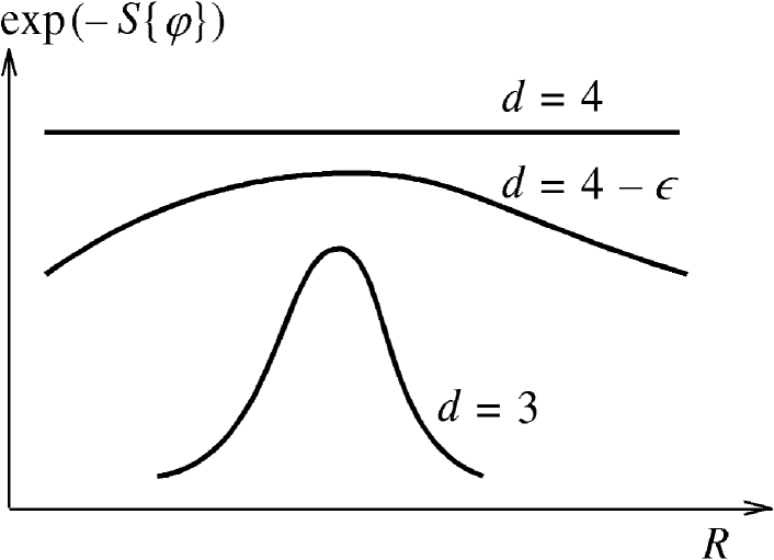
Figure 6:   Dependence of the integrand (1) on the instanton radius in $d$-dimensional $\varphi^{4}$ theory.

For $d$ significantly smaller than 4 (for example, $d=3$), the integrand $\exp(-S\{\varphi\})$ has a sharp maximum as a function of $R$ and allows saddle-point integration; when $d=4-\epsilon$ the maximum becomes gently sloping, and when $d=4$ the instanton action $S\{\varphi_{c}\}$ does not depend on $R$ at all. In the latter case the integral diverges, leading to the logarithmic situation. We see (see the curve for $d=4-\epsilon$ in Fig. 6) that the “activation” of renormalon contributions is, in fact, related to the appearance of slow tails in the integral (3), but these tails are taken into account in the Lipatov technique [36].

One can be puzzled by a following question. If the Lipatov technique is based on a saddle-point method, then how can it cover the definitely nonsaddle-point situation for $d=4-\epsilon$? The fact is that the saddle point in a functional integral practically never reduces to a simple maximum achieved at a single point: the maximum is degenerate in a certain space of finite dimensionality. Accordingly, a finite number of integrations should be performed exactly, rather than in the saddle-point approximation. However, if the integration is performed exactly over a certain variable (for example, $R$), it is of no significance whether the degeneracy is exact ($d=4$) or approximate ($d=4-\epsilon$). Nevertheless, in the latter case technical difficulties arise, and the corresponding methods (constrained instantons [41, 42]) have been poorly developed hitherto [36].

It is thus clear that even in cases where slow tails actually appear in the integral (3), the Lipatov procedure is sufficiently flexible and contains broad possibilities for dealing with them.

3. The limit $n\rightarrow\infty$.

There is an opinion that the significance of renormalon contributions can easily be proved by treating the $n$-component $\varphi^{4}$ theory in the limit $n\rightarrow\infty$ (and the analogous models in QCD and electrodynamics) [16]: the factor $n$ corresponds to a closed loop, and renormalon graphs containing the maximum possible number of loops are singled out by the large parameter $n$. Although diagrams of the same order, but with a smaller number of loops, can make comparable contributions at large $N$ due to the combinatorial factors, they have a slower dependence on $n$; therefore, the renormalons cannot be cancelled identically.

This argument is valid in any finite order of $1/n$. However, a detailed investigation of the structure of the $1/n$-expansion [18, 19] reveals the presence of numerous cancellations, and although the situation cannot be totally elucidated, the question is not resolved on the level of simple arguments of the type indicated.

It is not difficult to identify the crux of the problem here. As an example, let us consider the self-energy $\Sigma(p,m)$ of $\varphi^{4}$ theory; it is clear from a diagrammatic analysis for $m=0$ and values of the momentum $p$ close to the ultraviolet cutoff $\Lambda$ that the $(N+1)$th expansion coefficient for $\Sigma(p,0)-\Sigma(0,0)$ has the form of a polynomial in $n$

$$p^{2}\{A_{N}(N)n^{N}+A_{N-1}(N)n^{N-1}+\ldots+A_{1}(N)n+A_{0}(N)\},$$

in which the coefficient $A_{N}(N)$ is specified by renormalon graphs:

$$A_{N}(N)={\rm const}\cdot\left(-\frac{1}{16\pi^{2}}\right)^{N}N!.$$

If it is assumed that the renormalon graphs are contained in the instanton contribution, the expression (16) should transform into the Lipatov asymptotics at large $N$ [see Eq. (130) in Ref. [43] for $M=1$ and $p\approx\Lambda$]:

$$p^{2}\alpha\beta^{n}N^{(n+6)/2}\left(-\frac{1}{8\pi^{2}}\right)^{N}N!\left[\Gamma\left(\frac{n+2}{2}\right)\right]^{-1}\int\limits_{0}^{\infty}dy\,y^{(n+5)/3}K_{1}(y)^{2},$$

where $\alpha,\beta\sim 1$, and $K_{1}(x)$ is the McDonald function. It is easily seen that an equality between (16) and (18) is impossible when $n\rightarrow\infty$. This is a manifestation of the “noncancelability” of renormalons.

However, the usual condition for applicability of the Lipatov technique, $N\gg 1$ at large $n$ is, generally speaking, replaced by a more rigid condition, for example, $N\gg n$, and $n$ then has a bound of the type

$$n\mathbin{\lower 3.0pt\hbox{$\hbox to0.0pt{\raise 5.0pt\hbox{$\char 60\relax$}\hss}\mathchar 29208\relax$}}n_{0}(N),$$

which precludes going to the limit $n\rightarrow\infty$. If it is taken into account that the Lipatov asymptotics has limited accuracy (${\sim}1/N$ in relative units), the correct formulation of the question is as follows. Can we construct an interpolation polynomial of type (16) with the high-order coefficient (17) which would approximate the function (18) within an assigned accuracy in the interval $0\leq n\leq n_{0}(N)$, where $n_{0}(N)\rightarrow\infty$ as $N\rightarrow\infty$? The answer to this question is positive (see the Appendix); therefore, the assumption that the renormalon graphs are contained in the instanton contribution does not lead to contradictions.

4. Relationship to a Landau pole [16, 19].

It is easy to see (Fig. 2,c) that the summation of a sequence of renormalon diagrams corresponds to “dressing” the interaction. The relationship between the renormalized charge $g$ and the bare charge $g_{0}$ is then given by the familiar expression [44, 45, 46]

$$g_{0}=\frac{g}{1-\beta_{0}g\ln(\Lambda^{2}/m^{2})},$$

which contains a pole at the point

$$\Lambda_{c}^{2}=m^{2}e^{1/\beta_{0}g}.$$

Under the literal understanding of this pole in the spirit of the early papers by Landau and Pomeranchuk [17], a simple physical interpretation can be given to renormalon singularities (Refs. [16] and [19]). 

The dependence of the perturbation series on the cutoff parameter $\Lambda$ has the structure

$$c_{-1}\Lambda^{2}+c_{0}\ln\Lambda^{2}+c_{1}\Lambda^{-2}+c_{2}\Lambda^{-4}+\ldots+c_{n}\Lambda^{-2n}+\ldots.$$

The first two terms are eliminated by a renormalization procedure, and the rest terms, in principle, remain, but vanish in the limit $\Lambda\rightarrow\infty$. Because of the pole in (20), values of $\Lambda$ greater than $\Lambda_{c}$ are inaccessible in principle, and unremovable uncertainties of the type

$$\Lambda_{c}^{-2n}=m^{2}e^{-n/\beta_{0}g}$$

appear in the theory. Similar uncertainties are generated by renormalon singularities, whose existence on the positive semiaxis leads to ambiguity in the choice of the integration contour in the Borel integral (6). The contour can be drawn to the right or the left of the $n$th singularity (Fig. 7), producing an

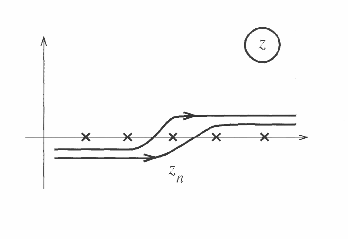
Figure 7:   Ambiguity of the choice of the integration path in the Borel integral (6) in the presence of renormalon singularities.

uncertainty in reconstructing the function from its Borel transform:

$$\delta F(g)\sim\oint\limits_{z\approx z_{n}}dz\,e^{-z/g}B(z)\sim e^{-z_{n}/g},$$

which, with consideration of the equality $z_{n}=n/\beta_{0}$ coincides with (23).

Of course, the literal interpretation of the Landau pole seems archaic, but after some modification of the argument presented, a real meaning can be assigned to it. It is well known [46], that the dependence of the charge $g$ on the distance scale $\Lambda^{-1}$ is given by the equation

$$\frac{dg}{d\ln\Lambda^{2}}=\beta(g)=\beta_{0}g^{2}+\beta_{1}g^{3}+\ldots,$$

whose solution depends drastically on the behavior of the Gell-Mann–Low function $\beta(g)$. The pole in (20) is eliminated, if $\beta(g)$ changes sign or behaves as $g^{\alpha}$ with $\alpha<1$ at large $g$. If, on the other hand, $\beta(g)$ is positive and increases as $g^{\alpha}$ with $\alpha>1$ when $g\rightarrow\infty$, the pole is preserved, and the theory is internally inconsistent because it is impossible to determine $g(\Lambda)$ for all $\Lambda$ (Ref. [46]). In the latter case the position of the pole is given by the equation

$$\ln\frac{\Lambda_{c}^{2}}{m^{2}}=\int\limits_{g}^{\infty}\frac{dx}{\beta(x)},$$

which, for small values of $g$, leads to the result

$$\Lambda_{c}^{2}={\rm const}\cdot m^{2}e^{1/\beta_{0}g},$$

which differs from (21) only by an insignificant constant factor. Thus, the existence of renormalon singularities seems fairly convincing for internally inconsistent theories. Conversely, there is no reason for them in “good” theories. 

Since the behavior of the function $\beta(g)$ at $g\mathbin{\lower 3.0pt\hbox{$\hbox to0.0pt{\raise 5.0pt\hbox{$\char 62\relax$}\hss}\mathchar 29208\relax$}}1$ is unknown, the presence or absence of renormalon singularities is a matter of belief. We stress, however, the following point. Factorial contributions of individual diagrams exist in all field theories in which the expansion of the $\beta$ function (25) begins from the quadratic term: then the interaction on the $k^{-1}$ scale is described by a formula of the type (20) with the replacement of $\Lambda$ by $k$, whose expansion gives $(\beta_{0}\ln k^{2})^{N}$ in the $N$th order [see (13)].   To resolve the question of the internal inconsistency of a theory, one should know all the coefficients in the expansion (25). Therefore, it would be incorrect to consider the formal existence of renormalon contributions as an indication of the internal inconsistency of a theory.

3. ANALYTIC PROPERTIES OF THE BOREL TRANSFORMS OF $\varphi^{4}$ THEORY

3.1. Expansion of the class of Borel transformations

For the ensuing treatment it is convenient to expand the class of Borel transformations, setting

$$F(g)=\int\limits_{0}^{\infty}dx\,e^{-x}x^{b_{0}-1}B(gx),$$

$$B(g)=\sum\limits_{N=0}^{\infty}\frac{F_{N}}{\Gamma(N+b_{0})}g^{N}$$

with the arbitrary parameter $b_{0}>0$, instead of (6) and (7). If $B(g)$ and $\tilde{B}(g)$ are the Borel transforms corresponding to the parameters $b_{0}$ and $b_{1}$ (for definiteness, we set $b_{1}>b_{0}$), it is not difficult to derive the conversion formula:

$$\tilde{B}(g)=\frac{1}{\Gamma(b_{1}-b_{0})}\int\limits_{0}^{\infty}dx\,\frac{x^{b_{1}-b_{0}-1}}{(1+x)^{b_{1}}}B\left(\frac{g}{1+x}\right).$$

We define the analyticity region of $B(g)$ by constructing the so-called Mittag–Leffler star [30], i.e., by drawing cuts from all singular points to infinity along rays drawn through these points from the origin of coordinates. If $g$ lies in the analyticity region of $B(g)$, the integration path in (29) does not pass through its singularities and $\tilde{B}(g)$ is also analytic. If $g_{c}$ is a singular point of $B(g)$, the integration path in (29) for $g=g_{c}$ unavoidably passes through $g_{c}$, generating a singularity in $\tilde{B}(g)$. For the interesting case of power-law singularities we have the correspondence rules

$$B(g)=A\Gamma(-\beta)\left(\frac{g_{c}-g}{g_{c}}\right)\rightarrow\tilde{B}(g)=A\Gamma(-\beta-b_{1}+b_{0})\left(\frac{g_{c}-g}{g_{c}}\right)^{\beta+b_{1}-b_{0}}$$

for noninteger $\beta+b_{1}-b_{0}$ and

$$B(g)=A\Gamma(-\beta)\left(\frac{g_{c}-g}{g_{c}}\right)^{\beta}\rightarrow\tilde{B}(g)=A\frac{(-1)^{n+1}}{n!}\left(\frac{g_{c}-g}{g_{c}}\right)^{n}\ln\left(\frac{g_{c}-g}{g_{c}}\right),$$

if $\beta+b_{1}-b_{0}=n$ is an integer.

We see that the analyticity region for all the Borel transforms is identical and that it is sufficient to establish it for any fixed $b_{0}$. The choice $b_{0}=1/2$ is convenient for investigating functional integrals, since a simple result is obtained in that case for the Borel transform of an exponential function:

$$F(g)=g^{-g}\rightarrow B(g)=\frac{\cos(2\sqrt{g})}{\sqrt{\pi}}=\frac{1}{2\sqrt{\pi}}\{\exp(2i\sqrt{g}+{\rm c.c.}\},$$

which preserves its exponential form. This permits writing an explicit expression for the Borel transform of the functional integral (1):

$$B_{I}(g)=\frac{1}{2\sqrt{\pi}}\int D\varphi\exp(-S_{0}\{\varphi\})\left[\exp\left(2i\sqrt{gS_{\rm int}\{\varphi\}}\right)+{\rm c.c.}\right].$$

The integrand is a regular function, and the analyticity region of $B_{I}(g)$ is determined by the condition for convergence of the integral.

3.2. Analyticity outside the negative semiaxis

For simplicity, let us consider scalar $\varphi^{4}$ theory. Generalization to the $n$-component case is trivial and reduces to only some complication of the notation. We assume that $m^{2}>0$, bearing in mind the subsequent analytic continuation to arbitrary complex $m^{2}$.

The integral (33) for $\varphi^{4}$ theory is defined well for positive values of $g$, since its convergence is determined by an exponential function of $-S_{0}\{\varphi\}$ and is obvious after the Fourier transformation of $\varphi(x)$:

$$S_{0}\{\varphi\}=\frac{1}{2}\int d^{d}x\,\{(\nabla\varphi)^{2}+m^{2}\varphi^{2}\}=\frac{1}{2}\sum\limits_{k}(k^{2}+m^{2})|\varphi_{k}|^{2}.$$

For the analytic continuation to complex $g$ we turn the integration path in (33), setting

$$g=\tilde{g}e^{i\Psi},\ \ \varphi=\tilde{\varphi}e^{-i\Psi/4},$$

where $\tilde{g}$ and $\tilde{\varphi}$ are real, and $\tilde{g}>0$. Then the integral in (33) takes the form

$$\int D\tilde{\varphi}\exp\left(-S_{0}\{\tilde{\varphi}\}e^{-i\Psi/2}\right)\left[\exp\left(2i\sqrt{\tilde{g}S_{\rm int}\{\tilde{\varphi}\}}\right)+{\rm c.c.}\right]$$

and converges for $-\pi<\Psi<\pi$. Thus, the Borel transform is analytic outside the negative semiaxis.

3.3. Analyticity within a circle

We utilize the formal technique used in Refs. [3] and [41] and introduce the function

$$R\{\varphi\})=\frac{S_{0}\{\varphi\}^{2}}{4S_{\rm int}\{\varphi\}}.$$

Then (33) is rewritten in the form

$$B_{I}(g)=\frac{1}{2\sqrt{\pi}}\int D\varphi\exp\left(-\left[1-i\left(\frac{g}{R\{\varphi\}}\right)^{1/2}\right]S_{0}\{\varphi\}\right)+{\rm c.c.},$$

and after the replacement of $R\{\varphi\}$ by the constant $R_{0}$, it is analytic within the circle $|g|<R_{0}$. Let us now suppose that

$$R\{\varphi\}\geq R_{0}$$

for all $\varphi$, i.e., $R_{0}$ is the exact lower bound of $R\{\varphi\}$. Setting $g=-|g|e^{i\gamma}$ ($-\pi\leq\gamma\leq\pi$), we have the inequality

$$|B_{I}(g)|\leq\frac{1}{2\sqrt{\pi}}\int D\varphi\left\{\exp\left(-\left[1-\left|\frac{g}{R\{\varphi\}}\right|^{1/2}\cos\frac{\gamma}{2}\right]S_{0}\{\varphi\}\right)+\exp(-S_{0}\{\varphi\})\right\},$$

which ensures convergence of the integral in (33) and, consequently, its analyticity within the circle $|g|<R_{0}$.

To find $R_{0}$, we consider the variational problem of minimizing $R\{\varphi\}$. It yields the equation

$$-\Delta\varphi(x)+m^{2}\varphi(x)-C\varphi^{3}(x)=0.$$

where

$$C=\frac{S_{0}\{\varphi\}}{2S_{\rm int}\{\varphi\}},$$

which, after the replacement $\varphi(x)\rightarrow\varphi(x)/\sqrt{C}$, transforms into the standard equation of an instanton of $\varphi^{4}$ theory. Using it, we can easily show that $R_{0}=S\{\varphi_{c}\}$, which establishes the required analyticity region (Fig. 3,b). Questions concerning the absence of instantons in massive four-dimensional theory [47] are discussed in Sec. 3.5.

Apart from the integral (1), some other functional integrals containing products of the type $\varphi(x_{1})\varphi(x_{2})\ldots\varphi(x_{M})$ in the preexponential factor are of interest. The presence of such products does not influence the convergence, and all the proofs performed remain unchanged.

3.4. Invariance relative to algebraic operations

As ’t Hooft pointed out [15], the singularities of Borel transforms are not shifted when algebraic operations are performed on the original functions. This can easily be proved for a modified definition of the Borel transform (10), which differs from (6) and (28), since

$$F(g)=F_{0}+F_{1}g+F_{2}g^{2}+F_{3}g^{3}+\ldots,\ \ B(z)=F_{0}\delta(z)+\frac{F_{1}}{0!}+\frac{F_{2}}{1!}z+\frac{F_{3}}{2!}z^{2}+\ldots$$

and $B(z)$ contains a $\delta$-function singularity at zero. The transformation of (10) by means of the replacement $g\rightarrow 1/z$ reduces to a Laplace transformation and allows inversion. It can be used to express the Borel transform of the product $F_{3}(g)=F_{1}(g)F_{2}(g)$ in terms of the known Borel transforms of the factors:

$$B_{3}(z)=\int\limits_{0}^{z}dz^{\prime}\,B_{1}(z^{\prime})B_{2}(z-z^{\prime}).$$

It can easily be seen that the $\delta$-function singularity in $B_{3}(z)$ corresponds to the definition (42) and that the singular points for finite $z$ coincide with the singular points of $B_{1}(z)$ and $B_{2}(z)$ (see the analogous reasoning in Sec. 3.1). In particular, the Borel transform $g^{n}$ is the function $z^{n-1}/\Gamma(n)$, which is analytic for integer values of $n$, and multiplication of the function by $g^{n}$ does not alter its analytic properties in the Borel plane.

If $F_{2}(z)=1/F_{1}(z)$, then

$$\delta(z)=\int\limits_{0}^{z}dz^{\prime}\,B_{1}(z^{\prime})B_{2}(z-z^{\prime})$$

and the $\delta$-function singularity on the left-hand side cancels out with the $\delta$-function singularities in $B_{1}(z)$ and $B_{2}(z)$. At finite values of $z$ the right-hand side contains singularities corresponding to singular points of $B_{1}(z)$ and $B_{2}(z)$, which are absent on the left-hand side and, therefore, compensate one another. This is possible only if $B_{2}(z)$ has singularities at the same points as $B_{1}(z)$.

The proof of the analogous statements for linear operations, viz., summation, differentiation, integration, etc., is trivial.

The standard definition of the Borel transform (6) is obtained from (10) and (42) when $F_{0}=0$ after the replacement $F(g)\rightarrow gF(g)$. In this case the $\delta$-function singularities disappear, and the remaining singularities are preserved at the same points due to the insignificance of the multiplier $g$. The definition (6) corresponds to the definition (28) with $b_{0}=1$, and, by virtue of Sec. 3.1, the analysis performed can be extended to arbitrary $b_{0}$.

Since all the quantities entering into the theory, viz. the Green’s functions, vertex parts, etc., can be expressed in terms of functional integrals with identical analytic properties (see the end of Sec. 3.3) using a finite number of algebraic operations, their singular points in the Borel plane are the same as for the integral (1).

3.5. Renormalization procedure

The absence of ultraviolet divergences was implicitly assumed above. In $\varphi^{4}$ theory this is correct for $d<2$. For $2\leq d\leq 4$ a continual theory without divergences can be constructed by introducing counterterms into the Lagrangian [46, 50]. In the simple case where only renormalization of the mass is required ($2\leq d<4$) the corresponding term in (4) is rewritten in the form

$$m_{0}^{2}\varphi^{2}=(m^{2}+\Delta m^{2})\varphi^{2}=(m^{2}+Ag+Bg^{2}+Cg^{3}+\ldots)\varphi^{2},$$

where the coefficients $A,B,C,\ldots$ are chosen so as to cancel the divergences. When counterterms are present, the analytic properties of integrals of the type (1) become more complicated, since the coupling constant appears not only in the combination $g\varphi^{4}$, but also in the form of $g\varphi^{2}$, $g^{2}\varphi^{2}$, etc. One of the directions of renormalon-related activity involved specifically the introduction of additional terms into the Lagrangian and tracing the renormalon singularities appearing [16, 18, 19]. A question arises in regard to the cancellation of singularities in the case when the coefficients in front of the additional terms are selected so as to remove divergences, for which an unequivocal answer could not be obtained.

A simpler route is to explicitly introduce regularization and to use renormalization-group equations. Here we have in mind the so-called cutoff scheme [51]: the vertex parts are calculated perturbatively as functions of the bare charge $g_{0}$ and the cutoff parameter $\Lambda$, then scaling functions which depend only on $g_{0}$ are obtained, and, finally, renormalized vertices, which depend on the renormalized charge $g$, are constructed [50]. In this case the explicit introduction of counterterms is not required, but all the details associated with their presence are taken into account, since the fundamental possibility of eliminating the divergences is essentially used to write the renormalization-group equations.

The simplest way of regularization consists of substituting $\varphi\epsilon(\hat{p})\varphi$, where $\hat{p}$ is the momentum operator, for the term $(\nabla\varphi)^{2}$ in (4), which is brought into the form $-\varphi\Delta\varphi=\varphi\hat{p}^{2}\varphi$. If

$$\epsilon(p)=\epsilon(-p),\ \ \epsilon(p)\geq 0,$$

then both the entire structure of the instanton calculations [49] and the proofs presented above are preserved. The only change occurs in the equation of the instanton (41), which is brought into the form

$$\epsilon(\hat{p})\varphi(x)+m^{2}\varphi(x)-\varphi^{3}(x)=0.$$

When the regularization

$$\epsilon(p)=p^{2}+p^{6}/\Lambda^{4}$$

is employed, the dependence of the action $S\{\varphi\}$ on the instanton radius $R$ in four-dimensional $\varphi^{4}$ theory has the form shown in Fig. 8.  

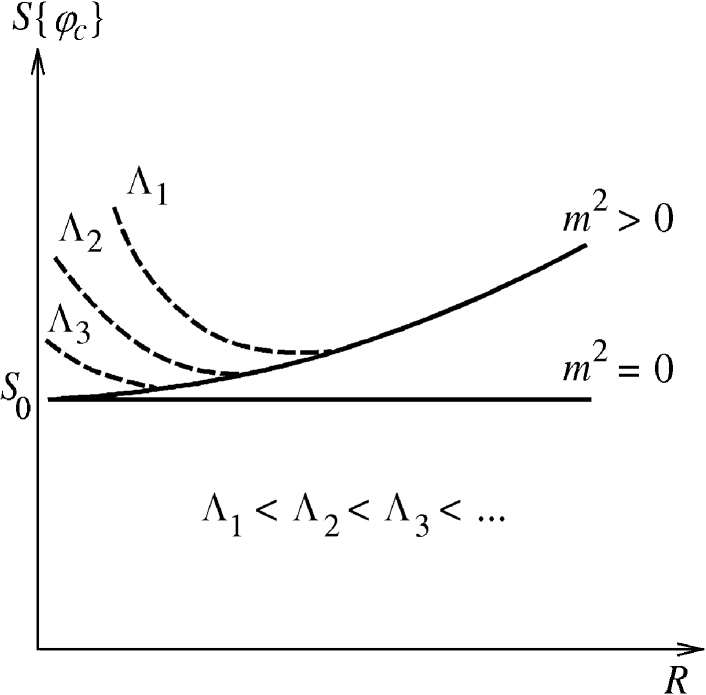
Figure 8:   Dependence of the action $S\{\varphi\}$ on the instanton radius $R$ in four-dimensional $\varphi^{4}$ theory in the absence of regularization (solid curves) and for a finite cutoff parameter $\Lambda$ (dashed lines).

If $\Lambda=\infty$, there is degeneracy with respect to the instanton radius in the massless theory [1], while there are no instantons in the massive theory [49] because of the monotonic dependence of $S\{\varphi\}$ on $R$. At finite values of $\Lambda$ a minimum appears on the plot of $S\{\varphi\}$ versus $R$ at $m^{2}>0$ (the dashed curves in Fig. 8), and instantons appear in the massive theory. Their action $S\{\varphi_{c}\}$ determines the positions of the singularities in the Borel plane. For $\Lambda\rightarrow\infty$ and arbitrary $m^{2}>0$ the value of $S\{\varphi_{c}\}$ tends to the instanton action of the massless theory, and the positions of the singularities do not depend on $m$. 

The renormalization-group equations (in the Callan–Symanzik form) are valid for the vertices $\Gamma^{L,N}$ with $N$ free tails and $L$ two-line insertions [50]:

$$\left[\frac{\partial}{\partial\ln\Lambda^{2}}+\beta(g_{0})\frac{\partial}{\partial g_{0}}+\left(L-\frac{N}{2}\right)\eta(g_{0})-L\eta_{2}(g_{0})\right]\Gamma^{L,N}(g_{0},\Lambda)=0.$$

Writing out three such equations with different $L$ and $N$, we can express the scaling functions $\beta(g_{0})$, $\eta(g_{0})$, and $\eta_{2}(g_{0})$ in terms of the vertices $\Gamma^{L,N}(g_{0},\Lambda)$ using algebraic operations, which do not shift the positions of the singularities in the Borel plane. In the limit $\Lambda\rightarrow\infty$, where Eq. (49) is valid, the dependence of the scaling functions on $\Lambda$ disappears [50], and their singularities in the Borel plane correspond to the massless theory.

The Gell-Mann–Low function $\beta(g_{0})$ defines the relationship between the renormalized charge $g$ and the bare charge $g_{0}$. Let the functions $F_{0}$ and $F_{1}$ be such that $F_{0}(g_{0})\equiv F_{1}(g)$. The relationship between the corresponding Borel transforms $B_{0}$ and $B_{1}$ [in the sense of the definition (10)] can easily be found for an infinitesimal charge transformation, $g_{0}=g+2\beta(g)\delta\Lambda/\Lambda$ [see (25)]:

$$B_{1}(z)=B_{0}(z)+\frac{2\delta\Lambda}{\Lambda}\int\limits_{0}^{z}dy\,[B_{0}(y)+yB^{\prime}_{0}(y)]B_{\beta}(z-y),$$

where $B_{\beta}(z)$ is the Borel transform of the function $\beta(g)/g$. Equation (50) is analogous to Eq. (43); therefore, the analytic properties do not change in the course of the charge transformation.

The vertices $\Gamma^{L,N}$ diverge as $\Lambda\rightarrow\infty$, but they become finite after separation of the divergent $Z$ factors from them and the transition from the bare to the renormalized charge. Since the $Z$ factors are, in turn, expressed in terms of the vertices $\Gamma^{L,N}$ (Ref. [50]), the renormalized vertices have the required analytic properties.

The dependence of the scaling functions on the renormalization scheme is given by the following conversion formulas [51]:

$$\tilde{\beta}(q(g))=\beta(g)\frac{dq(q)}{dg},$$

$$\tilde{\eta}(q(g))=\eta(g)-\beta(g)\frac{d\ln p(q)}{dg},$$

$$\tilde{\eta}_{2}(q(g))=\eta_{2}(g)-\beta(g)\frac{d\ln p_{2}(q)}{dg}.$$

The conversion functions $q(g)$, $p(g)$, and $p_{2}(g)$ for standard renormalization schemes (subtraction, cutoff etc.) are expressed in terms of the vertices $\Gamma^{L,N}$. Therefore, the analytic properties of the scaling functions are identical in all the schemes. In the general case the analytic properties of the conversion functions require additional investigation.

4. CONCLUSION

The results in Sec. 3 rule out the existence of renormalon singularities in $\varphi^{4}$ theory. If the arguments in Sec. 2 regarding the relationship to a Landau pole are considered convincing, $\varphi^{4}$ theory cannot be internally inconsistent. The same conclusion can be drawn on the basis of solid-state applications: a reasonable model of a disordered system reduces exactly to $\varphi^{4}$ theory [36, 39], and the internal inconsistency of $\varphi^{4}$ theory would signify the impossibility, in principle, of obtaining a mathematical description of this model. Therefore, a revision of the results in Refs. [34] and [35], in which indications of the internal inconsistency of $\varphi^{4}$ theory were obtained on the basis of an approximate reconstruction of the Gell-Mann–Low function, is urgently needed.

The results of Sec. 3 refer only to $\varphi^{4}$ theory and cannot be extended directly to other field theories; however, along with the qualitative arguments in Sec. 2, they demonstrate the nonconstructiveness of the conception of renormalons as a whole. Therefore, it would be of interest to generalize the method of proof used in Sec. 3 to other cases.

In quantum chromodynamics (QCD) the renormalon doctrine presently prevails [20]–[30]. However, the specific details of QCD in this context have never been stressed. For example, ’t Hooft [15], speaking about QCD, gives explanations within $\varphi^{4}$ theory and quantum electrodynamics. In recent publications [26, 30] the term “naive nonabelianization” appeared, which essentially means neglecting the specific details of QCD. On the other hand, in QCD there is a special reason for the belief in renormalons, which has a purely phenomenological character. The analysis of experimental data leads to the conclusion that the contribution of the high orders has a momentum dependence ${\propto}1/q^{4}$ (Ref. [22]). This dependence can easily be obtained from renormalon graphs, but, as is generally assumed, it cannot be obtained within the instanton method. The latter is based on the results in Refs. [10] and [11], according to which the instanton contribution is proportional to $1/q^{18}$. However, it can easily be seen that a term ${\propto}1/q^{4}$ appeared in Refs. [10] and [11], but contained divergences which the authors found difficult to eliminate;  this term was “transported” to the renormalon sector with the reasoning that it “contributes to the renormalon singularity …rather than to the instanton one” (Ref. [10], p. 287). If there are no renormalon singularities, this contribution was simply discarded; therefore, no real calculation of the Lipatov asymptotics were made for QCD.

This work was stimulated by lengthy discussions with P. G. Sil’vestrov, whom we thank for opposing the renormalon doctrine, his critical remarks, and general assistance in acquaintance with the situation. We also thank B. L. Ioffe, L. N. Lipatov, and the participants in the seminars at the Institute of Physical Problems, the P. N. Lebedev Physics Institute, the Institute of Theoretical and Experimental Physics, and the St. Petersburg Nuclear Physics Institute for their interest in this work and useful discussions.

This work was carried out with financial support from the INTAS (Grant 96-0580) and the Russian Foundation for Basic Research (Project 96-02-19527).

Appendix
Construction of interpolation polynomial

The polynomial of degree $N$ which coincides with the function $f(x)$ at the points $x_{0},x_{1},x_{2},\ldots,x_{N}$, is defined by the Lagrange formula [53]:

$$P_{N}(x)=\sum\limits_{k=0}^{N}\frac{f(x_{k})}{\psi^{\prime}(x_{k})}\frac{\psi(x)}{(x-x_{k})},$$

$$\psi(x)=(x-x_{0})(x-x_{1})(x-x_{2})\ldots(x-x_{N}),$$

and the interpolation error is given by the expression

$$R_{N}(x)=f(x)-P_{N}(x)=\frac{f^{(N+1)}(\xi)}{(N+1)!}\psi(x),$$

where $\xi$ belongs to the interval $(x_{0},x_{N})$.

The function (18), which is of interest to us, behaves as $q^{n}$ at $n\mathbin{\lower 3.0pt\hbox{$\hbox to0.0pt{\raise 5.0pt\hbox{$\char 60\relax$}\hss}\mathchar 29208\relax$}}N$ with slowly varying $q$, so that $\ln q\sim\ln N$. Neglecting these slow variations and omitting the common multiplier in (16) and (18), we have

$$f(x)=q^{x},\ \ A_{N}\sim\frac{1}{6^{N}N^{3}}.$$

Taking into account that $|\psi(x)|\leq\Delta^{N+1}$ in the interval $0\leq x\leq\Delta$, we obtain

$$|R_{N}(x)|\leq\frac{(\ln q)^{N+1}q^{\Delta}}{(N+1)!}\Delta^{N+1},$$

and the interpolation error is small for

$$\Delta\mathbin{\lower 3.0pt\hbox{$\hbox to0.0pt{\raise 5.0pt\hbox{$\char 60\relax$}\hss}\mathchar 29208\relax$}}N/\ln N.$$

To investigate the dependence of the coefficient $A_{N}$ on the positions of the points $x_{k}$, we set $\psi(x)=\mathop{\rm Re}\psi(x+i0)$, and calculating $\ln\psi(x+i0)$ using the Euler–MacLaurin formula, for $\psi(x)$ we obtain the expression

$$\psi(x)=F(x)\sin G(x).$$

In particular, for the power-law arrangement of points

$$x_{k}=(k/N)^{\alpha}\Delta,\ \ k=0,1,\ldots,N,$$

at $\alpha\gg 1$ we have

$$F(x)=(-1)^{N}\sqrt{x(\Delta-x)}\exp\left\{N\left[\alpha(x/\Delta)^{1/\alpha}+\ln\Delta-\alpha\right]\right\},$$

$$G(x)=\pi N(x/\Delta)^{1/\alpha}.$$

For a high-order coefficient of the polynomial (A.1) we obtain

$$A_{N}=\sum\limits_{k=0}^{N}\frac{f(x_{k})}{\psi^{\prime}(x_{k})}\sim\exp\{(\alpha-\ln\Delta)N\}$$

(the sum is determined by the term with $k=1$), and for $\alpha\sim\ln N$ the coefficient $A_{N}$ can be factorially small or factorially large, depending on the relationship between $\alpha$ and $\ln\Delta$, so that the required value of (A4) falls in the range of variation. Thus, the required polynomial (16) exists in the interval $0\leq n\leq n_{0}$, where $n_{0}\sim N/\ln N$.

Translated by P. Shelnitz

References

- [1] L. N. Lipatov, Zh. Éksp. Teor. Fiz. 72, 411 (1977) [Sov. Phys. JETP 45, 216 (1977)]
- [2] E. Brezin, J. C. Le Guillou, and J. Zinn-Justin, Phys. Rev. D 15, 1544 (1977).
- [3] C. Itzykson, G. Parisi, and J. B. Zuber, Phys. Rev. Let. 38, 306 (1977).
- [4] A. P. Bukhvostov and L. N. Lipatov, Zh. Éksp. Teor. Fiz. 73, 1658 (1977) [Sov. Phys. JETP 46, 871 (1977)].
- [5] E. B. Bogomolny and V. A. Fateyev, Phys. Lett. B 71, 93 (1977); L. N. Lipatov, A. P. Bukhvostov, and E. I. Malkov, Phys. Rev. D 19, 2974 (1979).
- [6] G. Parisi, Phys. Lett. B 66, 382 (1977).
- [7] Large Order Behavior of Perturbation Theory, J. C. Le Guillou and J. Zinn-Justin (Eds.), Amsterdam (1990).
- [8] C. Itzykson, G. Parisi, and J. B. Zuber, Phys. Rev. D 16, 996 (1977); R. Balian, C. Itzykson, G. Parisi, and J. B. Zuber, Phys. Rev. D 17, 1041 (1978).
- [9] E. B. Bogomolny and V. A. Fateyev, Phys. Lett. B 76, 210 (1978).
- [10] I. I. Balitsky, Phys. Lett. B 273, 282 (1991).
- [11] S. V. Faleev and P. G. Silvestrov, Nucl. Phys. B 463, 489 (1996).
- [12] B. Lautrup, Phys. Lett. B 69, 109 (1977).
- [13] S. Chadha and P. Olesen, Phys. Lett. B 72, 87 (1977).
- [14] P. Olesen, Phys. Lett. B 73, 327 (1977).
- [15] G. ’t Hooft, in The Whys of Subnuclear Physics: Proceedings of the 1977 International School of Subnuclear Physics (Erice, Trapani, Sicily, 1977), A. Zichichi (Ed.), Plenum Press, New York (1979).
- [16] G. Parisi, Phys. Lett. B 76, 65 (1978); Nucl. Phys. B 150, 163 (1979).
- [17] G. Parisi, Phys. Rep. 49, 215 (1979).
- [18] F. David, Nucl. Phys. B 209, 433 (1982); 234, 237 (1984); 263, 637 (1986).
- [19] M. C. Bergere and F. David, Phys. Lett. B 135, 412 (1984).
- [20] A. H. Mueller, Nucl. Phys. B 250, 327 (1985).
- [21] G. B. West, Phys. Rev. Lett. 67, 1388 (1991).
- [22] V. I. Zakharov, Nucl. Phys. B 385, 452 (1992).
- [23] L. S. Brown and L. J. Yaffe, Phys. Rev. D 45, R398 (1992); L. S. Brown, L. J. Yaffe, and C. Zhai, Phys. Rev. D 46, 4712 (1992).
- [24] G. Grunberg, Phys. Lett. B 304, 183 (1993).
- [25] A. H. Mueller, Phys. Lett. B 308, 355 (1993).
- [26] M. Beneke et al., Phys. Lett. B 307, 154 (1993); 348, 513 (1995); Nucl. Phys. B 452, 563 (1995); 472, 529 (1996); Phys. Rev. D 52, 3929 (1995).
- [27] D. J. Broadhurst, Z. Phys. C 58, 339 (1993).
- [28] A. I. Vainstein and V. I. Zakharov, Phys. Rev. Lett. 73, 1207 (1994); Phys. Rev. D 54, 4039 (1996).
- [29] C. N. Lovett-Turner and C. V. Maxwell, Nucl. Phys. B 432, 147 (1994).
- [30] S. V. Faleev and P. G. Silvestrov, Nucl. Phys. B 507, 379 (1997).
- [31] G. H. Hardy, Divergent Series, Clarendon Press, Oxford (1949) [Russ. transl., IL, Moscow (1951)].
- [32] Yu. V. Sidorov, M. V. Fedoryuk, and M. I. Shabunin, Lectures on the Theory of Functions of Complex Variables [in Russian], Nauka, Moscow (1976).
- [33] V. S. Popov, V. L. Eletskiĭ, and A. V. Turbiner, Zh. Éksp. Teor. Fiz. 74, 445 (1978) [Sov. Phys. JETP 47, 232 (1978)].
- [34] D. I. Kazakov, O. V. Tarasov, and D. V. Shirkov, Teor. Mat. Fiz. 38, 15 (1979).
- [35] Yu. A. Kubyshin, Teor. Mat. Fiz. 58, (1984).
- [36] I. M. Suslov, Usp. Fiz. Nauk 168, 503 (1998) [Phys. Usp. 41, 441 (1998)].
- [37] G. Falkovich, I. Kolokolov, V. Lebedev, and A. Migdal, Phys. Rev. E 54, 4896 (1996).
- [38] J. C. Le Guillou and J. Zinn-Justin, Phys. Rev. Lett. 39, 95 (1977); Phys. Rev. B 21, 3976 (1980).
- [39] M. V. Sadovskiĭ, Usp. Fiz. Nauk 133, 223 (1981) [Sov. Phys. Usp. 24, 96 (1981)].
- [40] G. ’t Hooft, Phys. Rev. D 14, 3433 (1976).
- [41] Y. Frishman, Phys. Rev. D 19, 540 (1979).
- [42] I. Affleck, Nucl. Phys. B 191, 429 (1981).
- [43] I. M. Suslov, Zh. Éksp. Teor. Fiz. 111, 220 (1997).
- [44] l. D. Landau, A. A. Abrikosov, and I. M. Khalatnikov, Dokl. Akad. Nauk SSSR 95, 497, 773, 1177 (1954).
- [45] V. B. Berestetskii, E. M. Lifshitz, and L. P. Pitaevskii, Quantum Electrodynamics, Pergamon Press, Oxford (1982) [Russ. original, Nauka, Moscow (1980)].
- [46] N. N. Bogoliubov and D. V. Shirkov, Introduction to the Theory of Quantized Fields, 2nd Am. ed., Wiley, New York (1980) [Russ. original, Nauka, Moscow (1976)].
- [47] l. D. Landau and I. Ya. Pomeranchuk, Dokl. Akad. Nauk SSSR 102, 489 (1955).
- [48] I. T. Dyatlov, V. V. Sudakov, and K. A. Ter-Martirosian, Zh. Éksp. Teor. Fiz. 32, 77 (1957) [Sov. Phys. JETP 5, 631 (1957)].
- [49] V. G. Makhankov, Phys. Lett. A 61, 431 (1977).
- [50] E. Brezin, J. C. Le Guillou, and J. Zinn-Justin, in Phase Transitions and Critical Phenomena, Vol. 6, C. Domb and M. S. Green (Eds.), Academic Press, New York (1976).
- [51] A. A. Blalimirov and D. V. Shirkov, Usp. Fiz. Nauk 129, 407 (1979) [Sov. Phys. Usp. 22, 860 (1979)].
- [52] I. M. Suslov, Zh. Éksp. Teor. Fiz. 106, 560 (1994) [JETP 79, 307 (1994)].
- [53] A. O. Gel’fond, The Calculus of Finite Differences [in Russian], Nauka, Moscow (1967).