The Massive Thermal Basketball Diagram

Abstract

The “basketball diagram” is a three-loop vacuum diagram for a scalar field theory that cannot be expressed in terms of one-loop diagrams. We calculate this diagram for a massive scalar field at nonzero temperature, reducing it to expressions involving three-dimensional integrals that can be easily evaluated numerically. We use this result to calculate the free energy for a massive scalar field with a $\phi^{4}$ interaction to three-loop order.

I Introduction

One of the obstacles to making progress in thermal field theory is that the technology for explicit perturbative calculations is underdeveloped. The formalism of thermal field theory is sufficiently complicated that there are often theoretical issues that are difficult to resolve without explicit calculations. An example is the gluon damping rate, which in the conventional perturbative expansion is plagued by problems involving gauge invariance. A formal solution to the problem by the resummation of hard thermal loops was presented by Braaten and Pisarski in 1990 [1]. However, the solution was not widely accepted until the leading order expression for the damping rate was calculated explicitly [2].

Around 1994, there was a significant step forward in the calculational technology for massless theories. The first perturbative calculation in thermal field theory that was carried out to high enough order that the running of the coupling constant came into play was a calculation of the free energy of a massless scalar field theory to order $g^{4}$ by Frenkel, Saa, and Taylor in 1992 [3]. In 1994, there were several other calculations of the free energy to fourth order in the coupling constant: a calculation by Corianò and Parwani for QED [4] and completely analytic calculations by Arnold and Zhai [5] for a massless scalar theory (correcting an error in Ref. [3]) and for QCD. Arnold and Zhai [5] made a particularly significant contribution by showing how three-loop vacuum diagrams, such as the so-called “basketball diagram” labeled 2b in Fig. 1, could be evaluated analytically. These analytic calculations were then quickly extended to order $g^{5}$ for massless scalar theories [6, 7], abelian gauge theories [8, 9], and nonabelian gauge theories [10, 11]. These explicit calculations revealed that the weak coupling expansion has convergence problems whose severity had not previously been appreciated.

Calculations in theories that include massive particles at nonzero temperature are more difficult, because there is a second scale in the problem. The calculational technology for massive theories is much less well-developed than that for massless theories. In addition to the obvious applications to theories with massive particles, calculations with massive propagators may also be useful for massless theories. In such theories, some of the most important thermal corrections have the effect of generating masses for the massless particles. These corrections may be responsible for the poor convergence properties of the weak coupling expansion. One of the most promising methods for resumming these corrections in scalar field theories is “screened perturbation theory” proposed by Karsch, Patkós, and Petreczky [12]. This method involves adding and subtracting a mass term from the Lagrangian and treating the subtracted term as a perturbation. The integrals encountered in the screened perturbative expansion are those of the corresponding massive theory. Screened perturbation theory has been applied to the free energy at the two-loop level, and it seems to dramatically improve the convergence of the perturbative series [12]. To determine how effective this method is in resumming the large perturbative corrections, it is essential to calculate higher order corrections explicitly.

In this paper, we take a step forward in the calculational technology for massive field theories by evaluating the basketball diagram. The diagram cannot be evaluated analytically, but we reduce it to expressions that involve integrals that are at most three-dimensional and can easily be evaluated numerically. Using our result for this diagram, we calculate the free energy for the massive $\phi^{4}$ field theory through next-to-next-to-leading order in the coupling constant $g^{2}$.

II Basketball Diagram

The basketball diagram is the diagram labeled 2b in Fig. 1. At nonzero temperature $T$, it involves a three-fold sum-integral over Euclidean momenta:

$${\cal I}_{\rm ball}\;=\;\hbox{$\sum$}\!\!\!\!\!\!\int_{PQR}{1\over P^{2}+m^{2}}{1\over Q^{2}+m^{2}}{1\over R^{2}+m^{2}}{1\over(P+Q+R)^{2}+m^{2}}\;.$$ (1)

The Euclidean four-momentum is $P=({\bf p},p_{4}=2\pi nT)$, where $n$ is an integer, and its square is $P^{2}={\bf p}^{2}+p_{4}^{2}$. The sum-integral $\hbox{${\scriptstyle\Sigma}$}\!\!\!\!\int_{P}$ represents the sum over the Euclidean energies and the integral over the spatial momentum:

$$\hbox{$\sum$}\!\!\!\!\!\!\int_{P}\;=\;T\sum_{p_{4}}\,\int_{\bf p}\,.$$ (2)

We use dimensional regularization of the integral over ${\bf p}$ to cut off the ultraviolet divergences in the sum-integral. Our convention for the measure in the integral is

$$\int_{\bf p}\;=\;\left({e^{\gamma}\mu^{2}\over 4\pi}\right)^{\epsilon}\,\int{d^{3-2\epsilon}p\over(2\pi)^{3-2\epsilon}}\,,$$ (3)

where $3-2\epsilon$ is the number of spatial dimensions, $\gamma$ is Euler’s constant, and $\mu$ is an arbitrary momentum scale. The factor of $\mu^{2\epsilon}$ gives the dimensionally-regularized integral (1) dimensions of (energy)⁴.

A Decomposition into integrals

In order to evaluate the sum-integral (1), we first reduce it to integrals that contain factors of the Bose-Einstein distribution function $n(E)=1/(e^{\beta E}-1)$ with positive energy $E$. We use the method of Bugrij and Shadura [13] which expresses the coefficients of the Bose-Einstein factors in terms of S-matrix elements at zero temperature. This strategy was also used by Frenkel, Taylor and Saa [3] to evaluate the massless basketball diagram. Although the derivation by Bugrij and Shadura is lengthy, their final result can be obtained by making some simple substitutions in the expression (1). The sum-integrals over Euclidean momenta $P=({\bf p},p_{4})$ are replaced by integrals over Minkowski momenta $p=(p_{0},{\bf p})$: $\hbox{${\scriptstyle\Sigma}$}\!\!\!\!\int_{P}\longrightarrow-i\int_{p}$. The Euclidean propagators are replaced by the Minkowski propagators of the real-time formalism:

$${1\over P^{2}+m^{2}}\;\longrightarrow\;i\left({i\over p^{2}-m^{2}+i\varepsilon}+n(|p_{0}|)2\pi\delta(p^{2}-m^{2})\right),$$ (4)

where $p^{2}=p_{0}^{2}-{\bf p}^{2}$. The sum-integral (1) is then given by the real part of the resulting expression, which now involves a three-fold integral over Minkowski momenta. For some of the integration momenta, the energy appears in the argument of a Bose-Einstein distribution. It is convenient to Wick-rotate the remaining integration momenta back to Euclidean space: $\int_{p}\longrightarrow i\int_{P}$, where the measure of the dimensionally regularized integral over the Euclidean momentum $P$ is

$$\int_{P}\;=\;\left({e^{\gamma}\mu^{2}\over 4\pi}\right)^{\epsilon}\,\int{d^{4-2\epsilon}p\over(2\pi)^{4-2\epsilon}}\,.$$ (5)

Having carried out this procedure, the basketball diagram can be expressed as the sum of terms with different numbers of Bose-Einstein factors:

$$I_{\rm ball}\;=\;{\cal I}^{(0)}+4\,{\cal I}^{(1)}+6\,{\cal I}^{(2)}+4\,{\cal I}^{(3)}\,.$$ (6)

The term with four Bose-Einstein factors is purely imaginary and it vanishes when we take the real part. The other terms are

$${\cal I}^{(0)} = \int_{PQR}{1\over P^{2}+m^{2}}{1\over Q^{2}+m^{2}}{1\over R^{2}+m^{2}}{1\over(P+Q+R)^{2}+m^{2}}\;,$$ (7)

$${\cal I}^{(1)} = \int_{p}n\delta(p)\int_{QR}{1\over Q^{2}+m^{2}}{1\over R^{2}+m^{2}}{1\over(P+Q+R)^{2}+m^{2}}\Bigg{|}_{P^{2}=-m^{2}}\;,$$ (8)

$${\cal I}^{(2)} = {\rm Re}\int_{p}n\delta(p)\int_{q}n\delta(q)\int_{R}{1\over R^{2}+m^{2}}{1\over(P+Q+R)^{2}+m^{2}}\Bigg{|}_{(P+Q)^{2}=-(p+q)^{2}-i\varepsilon}\;,$$ (9)

$${\cal I}^{(3)} = {\rm Re}\int_{p}n\delta(p)\int_{q}n\delta(q)\int_{r}n\delta(r){(-1)\over(p+q+r)^{2}-m^{2}+i\varepsilon}\;,$$ (10)

where we have used the shorthand $n\delta(p)=n(|p_{0}|)2\pi\delta(p^{2}-m^{2})$.

B Zero thermal factors

We first consider the term ${\cal I}^{(0)}$, which is the integral for the zero-temperature basketball diagram. The poles in $\epsilon$ for this diagram have been calculated by Kastening [14] and by Chung and Chung [15]. The finite terms in the diagram can be obtained by following the strategy used in Appendix B of Ref. [7] to calculate the zero-temperature basketball diagram in three dimensions.

The diagram is first Fourier-transformed to coordinate space, which reduces it to an integral over a single coordinate $R$:

$${\cal I}^{(0)}=\int_{R}V^{4}(R)\,,$$ (11)

where the potential $V(R)$ is

$$V(R)\;=\;\left({e^{\gamma}\mu^{2}\over 4\pi}\right)^{\epsilon}{1\over(2\pi)^{2-\epsilon}}\left({m\over R}\right)^{1-\epsilon}K_{1-\epsilon}(mR)$$ (12)

and $K_{\nu}(z)$ is a modified Bessel function. The measure for the integration over $R$ is

$$\int_{R}\;=\;\left({e^{\gamma}\mu^{2}\over 4\pi}\right)^{-\epsilon}\int d^{4-2\epsilon}R\,.$$ (13)

After integrating over angles in $4-2\epsilon$ dimensions, the integral reduces to

$${\cal I}^{(0)}\;=\;{m^{4}\over(4\pi)^{6}}\left({e^{\gamma}\mu^{2}\over m^{2}}\right)^{3\epsilon}{32\over\Gamma(2-\epsilon)}\int_{0}^{\infty}dt~{}t^{-1+2\epsilon}K_{1-\epsilon}^{4}(2t)\,.$$ (14)

The $t\to 0$ region of the integral gives poles in $\epsilon$. The small-$t$ behavior of the Bessel function is given by the power-series expansion

$$K_{1-\epsilon}(2t)={\Gamma(1-\epsilon)t^{-1+\epsilon}\over 2}+{\Gamma(1-\epsilon)\Gamma(\epsilon)\over 2}\sum^{\infty}_{j=0}\left({t^{2j+1+\epsilon}\over(j+1)!\Gamma(j+1+\epsilon)}-{t^{2j+1-\epsilon}\over j!\Gamma(j+2-\epsilon)}\right).$$ (15)

In the integral over $t$ in (14), the poles in $\epsilon$ come from the $t^{-5+6\epsilon}$, $t^{-3+6\epsilon}$, $t^{-3+4\epsilon}$, $t^{-1+6\epsilon}$, $t^{-1+4\epsilon}$, and $t^{-1+2\epsilon}$ terms. We can calculate the poles analytically by multiplying each of these terms by an appropriate convergence factor and integrating over $t$. After these terms, with their convergence factors, are subtracted from the original integrand, the remaining integral is convergent for $\epsilon=0$ and can be evaluated numerically. We choose convergence factors of the form $(e^{8t})_{n}e^{-8t}$, where $(e^{x})_{n}$ is the truncated power series for the exponential function: $(e^{x})_{n}=\sum^{n}_{i=0}x^{i}/i!$. This convergence factor behaves like $1+{\cal O}(t^{n+1})$ at small $t$, and has the same exponential falloff as $K_{1}^{4}(2t)$ at large $t$. The resulting expression for the integral is in the limit $\epsilon\rightarrow 0$

$$\int^{\infty}_{0}dt~{}t^{-1+2\epsilon}K^{4}_{1-\epsilon}(2t)$$ (16)

$$\;=\;{\Gamma^{4}(1-\epsilon)\over 16}\int^{\infty}_{0}dt~{}t^{-1+2\epsilon}e^{-8t}\Bigg{[}t^{-4+4\epsilon}\left(e^{8t}\right)_{4}+{4t^{-2+2\epsilon}\over\epsilon}\left(t^{2\epsilon}-{\Gamma(1+\epsilon)\over\Gamma(2-\epsilon)}\right)\left(e^{8t}\right)_{2}$$ (17)

$$\qquad\qquad\qquad\qquad\qquad+{2t^{2\epsilon}\over\epsilon(1+\epsilon)}\left(t^{2\epsilon}-{2\Gamma(2+\epsilon)\over\Gamma(3-\epsilon)}\right)+{6\over\epsilon^{2}}\left(t^{2\epsilon}-{\Gamma(1+\epsilon)\over\Gamma(2-\epsilon)}\right)^{2}\Bigg{]}$$ (18)

$$\qquad\qquad\;+\;\int^{\infty}_{0}dt~{}{1\over t}\Bigg{\{}K_{1}^{4}(2t)-{e^{-8t}\over 16}\bigg{[}{1\over t^{4}}(e^{8t})_{4}+{4\over t^{2}}(2\log t+2\gamma-1)(e^{8t})_{2}$$ (19)

$$\qquad\qquad\qquad\qquad\qquad\qquad\qquad+2(2\log t+2\gamma-\mbox{${5\over 2}$})+6(2\log t+2\gamma-1)^{2}\bigg{]}\Bigg{\}}\,.$$ (20)

The first integral in (20) can be evaluated analytically in terms of gamma functions, and it reduces in the limit $\epsilon\to 0$ to

$$\Gamma(1+6\epsilon) \Bigg{\{}{1\over\epsilon^{3}}+{17\over 6\epsilon^{2}}+{59-36\pi^{2}\over 12\epsilon}-{821\over 24}+381\log 2$$ (22)

$$-90\log^{2}2-216\log^{3}2-{61\pi^{2}\over 6}-12\pi^{2}\log 2-27\psi^{\prime\prime}(1)\Bigg{\}}\,,$$

where $\psi(z)$ is the digamma function. The numerical value of the second integral in (20) is 0.36106. Inserting these results into (14) and keeping terms through order $\epsilon^{0}$, our final result is

$${\cal I}^{(0)}\;=\;{1\over(4\pi)^{6}}\left({\mu\over m}\right)^{6\epsilon}\left[{2\over\epsilon^{3}}+{23\over 3\epsilon^{2}}+{35+\pi^{2}\over 2\epsilon}+C_{0}\right]m^{4}\,,$$ (23)

where the numerical value of the constant is $C_{0}=39.429$.

C One thermal factor

The expression (8) for ${\cal I}^{(1)}$ can be written as

$${\cal I}^{(1)}\;=\;I_{\rm sun}(-m^{2})\int_{p}n(|p_{0}|)2\pi\delta(p^{2}-m^{2})\,,$$ (24)

where $I_{\rm sun}(P^{2})$ is the integral for the “setting sun diagram” in the boson self-energy at zero temperature:

$$I_{\rm sun}(P^{2})\;=\;\int_{QR}{1\over Q^{2}+m^{2}}{1\over R^{2}+m^{2}}{1\over(P+Q+R)^{2}+m^{2}}\,.$$ (25)

The integral over $p$ in (24) can be written as

$$\int_{p}n(|p_{0}|)2\pi\delta(p^{2}-m^{2})\;=\;{1\over(4\pi)^{2}}\left({\mu\over m}\right)^{2\epsilon}J_{1}T^{2}\;,$$ (26)

where $J_{1}$ is a function of $\beta m$ defined by (A.5) in the Appendix.

The setting-sun integral (25) at $P^{2}=-m^{2}$ can be evaluated by following the strategy used in Appendix B of Ref. [7] to calculate the corresponding integral in three dimensions. After Fourier-transforming, it reduces to an integral over a single coordinate $R$:

$$I_{\rm sun}(-m^{2})\;=\;\int_{R}e^{iP\cdot R}V^{3}(R)\Bigg{|}_{P^{2}=-m^{2}}\;.$$ (27)

After averaging over angles in $4-2\epsilon$ dimensions and evaluating at $P^{2}=-m^{2}$, the exponential factor becomes

$$\left\langle e^{iP\cdot R}\right\rangle\Bigg{|}_{P^{2}=-m^{2}}\;=\;\Gamma(2-\epsilon)\left({2\over mR}\right)^{1-\epsilon}I_{1-\epsilon}(mR)\,,$$ (28)

where $I_{\nu}(z)$ is a modified Bessel function. The integral over $R$ then reduces to a one-dimensional integral, and (27) becomes

$$I_{\rm sun}(-m^{2})\;=\;{m^{2}\over(4\pi)^{4}}\left({\mu\over m}\right)^{4\epsilon}16e^{2\gamma\epsilon}\int_{0}^{\infty}dt~{}t^{-1+2\epsilon}I_{1-\epsilon}(2t)K_{1-\epsilon}^{3}(2t).$$ (29)

The $t\to 0$ region of the integral gives poles in $\epsilon$. The small-$t$ behavior of the Bessel function $I_{1-\epsilon}(2t)$ is given by the power-series expansion

$$I_{1-\epsilon}(2t)\;=\;\sum^{\infty}_{j=0}{t^{2j+1-\epsilon}\over j!\Gamma(j+2-\epsilon)}\,.$$ (30)

In the integral over $t$ in (29), the poles in $\epsilon$ come from the $t^{-3+4\epsilon}$, $t^{-1+4\epsilon}$, and $t^{-1+2\epsilon}$ terms. We can calculate the poles analytically by multiplying each of these terms by an appropriate convergence factor and integrating over $t$. After these terms, with their convergence factors, are subtracted from the original integrand, the remaining integral is convergent for $\epsilon=0$ and can be evaluated numerically. We choose convergence factors of the form $(e^{6t})_{n}e^{-6t}$. The resulting expression for the integral is in the limit $\epsilon\rightarrow 0$

$$\int^{\infty}_{0}dt~{}t^{-1+2\epsilon}~{}I_{1-\epsilon}(2t)~{}K^{3}_{1-\epsilon}(2t)$$ (31)

$$\;=\;{\Gamma^{2}(1-\epsilon)\over 8(1-\epsilon)}\int^{\infty}_{0}dt~{}t^{-1+2\epsilon}e^{-6t}\Bigg{[}t^{-2+2\epsilon}\left(e^{6t}\right)_{2}+{t^{2\epsilon}\over 2-\epsilon}+{3\over\epsilon}\left(t^{2\epsilon}-{\Gamma(1+\epsilon)\over\Gamma(2-\epsilon)}\right)\Bigg{]}$$ (32)

$$\qquad\qquad\;+\;\int^{\infty}_{0}dt~{}{1\over t}\Bigg{\{}I_{1}(2t)K_{1}^{3}(2t)-{e^{-6t}\over 8}\bigg{[}{1\over t^{2}}(e^{6t})_{2}+{1\over 2}+3(2\log t+2\gamma-1)\bigg{]}\Bigg{\}}\,.$$ (33)

The first integral in (33) can be evaluated analytically in terms of gamma functions, and it reduces in the limit $\epsilon\to 0$ to

$$\Gamma(1+4\epsilon)\Bigg{\{}-{3\over 4\epsilon^{2}}-{11\over 8\epsilon}-{167\over 16}+{5\over 2}\log 6+3\log^{2}6+{3\pi^{2}\over 2}\Bigg{\}}\,.$$ (34)

The numerical value of the second integral in (33) is $-1.2713$. Inserting these results into (29) and keeping terms through order $\epsilon^{0}$, we obtain

$$I_{\rm sun}(-m^{2}) = {1\over(4\pi)^{4}}\left({\mu\over m}\right)^{4\epsilon}\left[-{3\over 2\epsilon^{2}}-{17\over 4\epsilon}+C_{1}\right]m^{2}\;,$$ (35)

where the numerical value of the constant is $C_{1}=-9.8424$. Inserting (35) and (26) into (24), our final result is

$${\cal I}^{(1)} = {1\over(4\pi)^{6}}\left({\mu\over m}\right)^{6\epsilon}\left[-{3\over 2\epsilon^{2}}-{17\over 4\epsilon}+C_{1}\right]J_{1}m^{2}T^{2}\;.$$ (36)

Note that the integral $J_{1}$ depends on $\epsilon$.

D Two thermal factors

The expression (9) for ${\cal I}^{(2)}$ involves the “bubble integral”

$$I_{\rm bubble}(P^{2})\;=\;\int_{R}{1\over R^{2}+m^{2}}{1\over(P+R)^{2}+m^{2}}\,,$$ (37)

which can be evaluated using a Feynman parameter:

$$I_{\rm bubble}(P^{2})\;=\;{1\over(4\pi)^{2}}\left({\mu\over m}\right)^{2\epsilon}\left[{1\over\epsilon}-\int_{0}^{1}dx\log{m^{2}+x(1-x)P^{2}\over m^{2}}\right]\;.$$ (38)

The real part of the integral evaluated at $P^{2}=-(p+q)^{2}-i\varepsilon$ is obtained by simply replacing the argument of the logarithm by its absolute value. When (38) is inserted into (9), the coefficient of $1/\epsilon$ can be evaluated using (26). Reducing the other term to an integral over spatial momenta, we obtain

$${\cal I}^{(2)} = {1\over(4\pi)^{6}}\left({\mu\over m}\right)^{6\epsilon}\Bigg{\{}{1\over\epsilon}J_{1}^{2}T^{4}-32\int_{0}^{\infty}dp\,{p^{2}n(E_{p})\over E_{p}}\int_{0}^{\infty}dq\,{q^{2}n(E_{q})\over E_{q}}$$ (40)

$$\hskip 142.26378pt\times\sum_{\sigma}\int_{0}^{1}dx\left\langle\log{|m^{2}-x(1-x)(E_{\sigma}^{2}-k^{2})|\over m^{2}}\right\rangle\Bigg{\}}\,,$$

where $E_{\sigma}=E_{p}+\sigma E_{q}$, $k=|{\bf p}+{\bf q}|$, the sum is over $\sigma=\pm$, and the angular brackets denote the average over the angles of ${\bf p}$ and ${\bf q}$. It is convenient to change the angular integration variable to $k$. The integral over $x$ in the angular average then reduces to

$$\int_{0}^{1}dx\left\langle\log{|m^{2}-x(1-x)(E_{\sigma}^{2}-k^{2})|\over m^{2}}\right\rangle\;=\;{1\over 2pq}\int_{|p-q|}^{p+q}dk~{}k~{}\left[f_{2}(E_{\sigma},k)-2\right]\,,$$ (41)

where the function in the integrand is

$$f_{2}(E,k) = \left({E^{2}-M_{k}^{2}\over E^{2}-k^{2}}\right)^{1/2}\log{(E^{2}-k^{2})^{1/2}+(E^{2}-M_{k}^{2})^{1/2}\over(E^{2}-k^{2})^{1/2}-(E^{2}-M_{k}^{2})^{1/2}}\,,\hskip 28.45274ptk^{2}<E^{2}-4m^{2}\,,$$ (42)

$$= 2\left({M_{k}^{2}-E^{2}\over E^{2}-k^{2}}\right)^{1/2}{\rm atan}\left({E^{2}-k^{2}\over M_{k}^{2}-E^{2}}\right)^{1/2}\,,\hskip 85.35826ptE^{2}-4m^{2}<k^{2}<E^{2}\,,$$ (43)

$$= \left({M_{k}^{2}-E^{2}\over k^{2}-E^{2}}\right)^{1/2}\log{(M_{k}^{2}-E^{2})^{1/2}+(k^{2}-E^{2})^{1/2}\over(M_{k}^{2}-E^{2})^{1/2}-(k^{2}-E^{2})^{1/2}}\,,\hskip 28.45274ptE^{2}<k^{2}\,.$$ (44)

and $M_{k}^{2}=4m^{2}+k^{2}$. Our final result is

$${\cal I}^{(2)} = {1\over(4\pi)^{6}}\left({\mu\over m}\right)^{6\epsilon}\left[\left({1\over\epsilon}+2\right)J_{1}^{2}+K_{2}\right]T^{4}\;,$$ (45)

where $K_{2}$ is the function of $\beta m$ defined by the following integral:

$$K_{2} = -{32\over T^{4}}\int_{0}^{\infty}dp\;{pn(E_{p})\over E_{p}}\int_{0}^{p}dq\;{qn(E_{q})\over E_{q}}\int_{p-q}^{p+q}dk\;k\;\sum_{\sigma}f_{2}(E_{\sigma},k)\;.$$ (46)

In the limit $m\to 0$, $K_{2}$ reduces to

$$K_{2}\;\longrightarrow\;-{(4\pi)^{4}\over 72}\left[\log{4\pi T\over m}-{1\over 2}-{\zeta^{\prime}(-1)\over\zeta(-1)}\right]\,,$$ (47)

where $\zeta(z)$ is the Riemann zeta function. In that same limit, $J_{1}$ reduces to

$$J_{1}\;\longrightarrow\;{(4\pi)^{2}\over 12}\left\{1+2\epsilon\left[-\log{4\pi T\over m}+1+{\zeta^{\prime}(-1)\over\zeta(-1)}\right]+O(\epsilon^{2})\right\}\,.$$ (48)

Inserting (47) and (48) into (45), we obtain the expression for ${\cal I}^{(2)}$ in the limit $m\to 0$:

$${\cal I}^{(2)}\;\longrightarrow\;{1\over 144(4\pi)^{2}}\left({\mu\over 4\pi T}\right)^{6\epsilon}\left[{1\over\epsilon}+7+6{\zeta^{\prime}(-1)\over\zeta(-1)}\right]\,.$$ (49)

This agrees with the analytic result first obtained by Frenkel, Saa, and Taylor [3].

E Three thermal factors

The integral ${\cal I}^{(3)}$ in (10) is finite in three spatial dimensions, so we can set $\epsilon=0$ from the beginning. After using the delta functions to integrate over $p_{0}$, $q_{0}$, and $r_{0}$, the integral reduces to

$${\cal I}^{(3)} = {128\over(4\pi)^{6}}\int_{0}^{\infty}dp\,{p^{2}n(E_{p})\over E_{p}}\int_{0}^{\infty}dq\,{q^{2}n(E_{q})\over E_{q}}\int_{0}^{\infty}dr\,{r^{2}n(E_{r})\over E_{r}}\sum_{\sigma,\tau}\left\langle{\cal P}{(-1)\over E_{\sigma\tau}^{2}-k^{2}-m^{2}}\right\rangle\,,$$ (50)

where $E_{\sigma\tau}=E_{p}+\sigma E_{q}+\tau E_{r}$, $k=|{\bf p}+{\bf q}+{\bf r}|$, the sum is over $\sigma=\pm$ and $\tau=\pm$, the angular brackets denote the average over the angles of ${\bf p}$, ${\bf q}$, and ${\bf r}$, and ${\cal P}$ denotes the principal value prescription for the poles in the propagator. Before averaging over the angles of ${\bf p}$, ${\bf q}$, and ${\bf r}$, it is convenient to use the symmetry in the integration variables to impose the restriction $r<q<p$ while multiplying by $3!$. We can then average over angles using the identity

$$\left\langle F(|{\bf p}+{\bf q}+{\bf r}|)\right\rangle\;=\;{1\over 4pqr}\int_{0}^{p+q+r}dk~{}k~{}w(p,q,r,k)~{}F(k)\,,$$ (51)

where the weight function for the case $r<q<p$ is

$$w(p,q,r,k) = 2k~{}\theta(q+r-p)\,,\hskip 42.67912pt0<k<|p-q-r|\,,$$ (52)

$$= k+q+r-p\,,\hskip 56.9055pt|p-q-r|<k<p+r-q\,,$$ (53)

$$= 2r\,,\hskip 113.81102ptp+r-q<k<p+q-r\,,$$ (54)

$$= p+q+r-k\,,\hskip 56.9055ptp+q-r<k<p+q+r\,.$$ (55)

Integrating over $k$, our final result is

$${\cal I}^{(3)}\;=\;{1\over(4\pi)^{6}}K_{3}T^{4}\,,$$ (56)

where $K_{3}$ is the function of $\beta m$ defined by the following integral:

$$K_{3}\;=\;{96\over T^{4}}\int_{0}^{\infty}dp\;{pn(E_{p})\over E_{p}}\int_{0}^{p}dq\;{qn(E_{q})\over E_{q}}\int_{0}^{q}dr\;{rn(E_{r})\over E_{r}}\sum_{\sigma\tau}\left[f_{3}(E_{\sigma\tau},p+q+r)\right.$$ (57)

$$\left.-f_{3}(E_{\sigma\tau},p+q-r)-f_{3}(E_{\sigma\tau},p-q+r)+f_{3}(E_{\sigma\tau},p-q-r)\right]\;.$$ (58)

The function in the integrand is

$$f_{3}(E,p) = p\log{m^{2}-E^{2}+p^{2}\over m^{2}}+2(m^{2}-E^{2})^{1/2}\;{\rm atan}{p\over(m^{2}-E^{2})^{1/2}}\;,\hskip 32.15175ptE^{2}<m^{2}\;,$$ (59)

$$= p\log{|E^{2}-m^{2}-p^{2}|\over m^{2}}+(E^{2}-m^{2})^{1/2}\;\log{(E^{2}-m^{2})^{1/2}+p\over|(E^{2}-m^{2})^{1/2}-p|}\;,\hskip 8.5359ptE^{2}>m^{2}\;.$$ (60)

The integral $K_{3}$ in the limit $m\to 0$ was calculated by Frenkel, Saa, and Taylor numerically [3] and by Arnold and Zhai analytically [5]:

$$K_{3}\;\longrightarrow\;{(4\pi)^{4}\over 48}\left[-{7\over 15}+{\zeta^{\prime}(-1)\over\zeta(-1)}-{\zeta^{\prime}(-3)\over\zeta(-3)}\right]\,.$$ (61)

Its numerical value in this limit is $K_{3}\to 453.51$.

F Total

The final result for the basketball diagram is obtained by inserting (23), (36), (45), and (56) into (6):

$${\cal I}_{\rm ball} = {1\over(4\pi)^{6}}\left({\mu\over m}\right)^{6\epsilon}\Bigg{\{}\left[{2\over\epsilon^{3}}+{23\over 3\epsilon^{2}}+{35+\pi^{2}\over 2\epsilon}+C_{0}\right]m^{4}+\left[-{6\over\epsilon^{2}}-{17\over\epsilon}+4C_{1}\right]J_{1}m^{2}T^{2}$$ (63)

$$\hskip 85.35826pt+\left({6\over\epsilon}+12\right)J_{1}^{2}T^{4}+(6K_{2}+4K_{3})T^{4}\Bigg{\}}\;.$$

To obtain the Laurent expansion including all terms through order $\epsilon^{0}$, it remains only to expand the factor $(\mu/m)^{6\epsilon}$ and the integral $J_{1}$ in powers of $\epsilon$. In the limit $m\to 0$, (63) reduces to the analytic result obtained by Arnold and Zhai [5]:

$${\cal I}_{\rm ball} \longrightarrow {1\over 24(4\pi)^{2}}\left({\mu\over 4\pi T}\right)^{6\epsilon}\left[{1\over\epsilon}+{91\over 15}+8{\zeta^{\prime}(-1)\over\zeta(-1)}-2{\zeta^{\prime}(-3)\over\zeta(-3)}\right]\,.$$ (64)

III Three-Loop Free Energy

Using our result for the massive basketball diagram, we can calculate the free energy for a massive scalar field theory with a $\phi^{4}$ interaction to three-loop order. The Lagrangian for the field theory is

$${\cal L}\;=\;{1\over 2}\partial_{\mu}\phi\partial^{\mu}\phi-{1\over 2}{\bar{m}}^{2}\phi^{2}-{1\over 24}{\bar{g}}^{2}\mu^{2\epsilon}\phi^{4}+\Delta{\cal L}\;,$$ (65)

where $\Delta{\cal L}$ includes the counterterms. We define the parameters ${\bar{m}}$ and ${\bar{g}}$ by dimensional regularization and minimal subtraction, so they depend implicitly on the renormalization scale $\mu$.

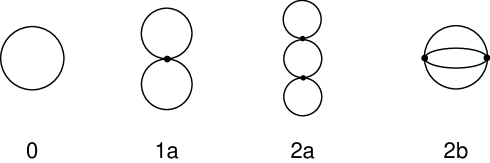
FIG. 1.: One-loop, two-loop, and three-loop diagrams contributing to the free energy.

A One loop

The free energy at zeroth order in $\bar{g}$ is given by the one-loop diagram labeled 0 in Fig. 1:

$${\cal F}_{0} = -{1\over 2}{\cal I}_{0}^{\prime}\,,$$ (66)

where the sum-integral ${\cal I}_{0}^{\prime}$ is defined by (A.1) in the Appendix. Keeping only the temperature-dependent term, the result for the one-loop contribution to the free energy is

$${\cal F}_{0} = -{1\over 2(4\pi)^{2}}\left({\mu\over\bar{m}}\right)^{2\epsilon}J_{0}T^{4}\;,$$ (67)

where $J_{0}$ is the function of $\beta\bar{m}$ defined in (A.5). In the limit $\epsilon\to 0$, this function reduces to

$$J_{0}\bigg{|}_{\epsilon=0}\;=\;{16\over 3T^{4}}\int_{0}^{\infty}dp\;{p^{4}\over E_{p}}n(E_{p})\;.$$ (68)

B Two loops

The free energy at second order in $\bar{g}$ comes from the two-loop diagram labeled 1a in Fig. 1, and also from inserting the order-$\bar{g}^{2}$ mass counterterm $\Delta_{1}m^{2}$ into the one-loop diagram:

$${\cal F}_{1} = {\cal F}_{\rm 1a}+{\partial{\cal F}_{0}\over\partial\bar{m}^{2}}\Delta_{1}m^{2}\,.$$ (69)

The expression for the diagram 1a is

$${\cal F}_{\rm 1a} = {1\over 8}\bar{g}^{2}{\cal I}_{1}^{2}\,,$$ (70)

where the sum-integral ${\cal I}_{n}$ is defined in (A.2). Keeping only the temperature-dependent terms, this diagram is

$${\cal F}_{\rm 1a} = {\bar{\alpha}\over 8(4\pi)^{2}}\left({\mu\over\bar{m}}\right)^{4\epsilon}\left[-2\left({1\over\epsilon}+1+O(\epsilon)\right)J_{1}\bar{m}^{2}T^{2}+J_{1}^{2}T^{4}\right]\,,$$ (71)

where $\bar{\alpha}=\bar{g}^{2}/(4\pi)^{2}$. The pole proportional to $J_{1}{\bar{m}}^{2}T^{2}$ is canceled by the last term in (69). The identity (A.6) is useful for calculating the derivative ${\partial J_{0}/\partial{\bar{m}}^{2}}$ in that term. The mass counterterm is thereby determined to be

$$\Delta_{1}m^{2} = {1\over 2\epsilon}\,\bar{\alpha}\,\bar{m}^{2}\,.$$ (72)

Our final result for the two-loop contribution to the free energy is

$${\cal F}_{1} = {\bar{\alpha}\over 8(4\pi)^{2}}\left[-2(\bar{L}+1)J_{1}\bar{m}^{2}T^{2}+J_{1}^{2}T^{4}\right]\;,$$ (73)

where $\bar{L}=\log(\mu^{2}/\bar{m}^{2})$ and $J_{1}$ is the function of $\beta\bar{m}$ defined in (A.5). In the limit $\epsilon\to 0$, it reduces to

$$J_{1}\bigg{|}_{\epsilon=0}\;=\;{8\over T^{2}}\int_{0}^{\infty}dp\;{p^{2}\over E_{p}}n(E_{p})\;.$$ (74)

C Three loops

The free energy at second order in $g^{2}$ comes from the three-loop diagrams labeled 2a and 2b in Fig. 1, and also from inserting counterterms into the one-loop and two-loop diagrams:

$${\cal F}_{2} = {\cal F}_{\rm 2a}+{\cal F}_{\rm 2b}+{\,\partial{\cal F}_{\rm 1a}\over\partial\bar{m}^{2}}\Delta_{1}m^{2}+{{\cal F}_{\rm 1a}\over\bar{g}^{2}}\Delta_{1}g^{2}+{1\over 2}{\partial^{2}{\cal F}_{0}\over(\partial\bar{m}^{2})^{2}}\left(\Delta_{1}m^{2}\right)^{2}+{\partial{\cal F}_{0}\over\partial\bar{m}^{2}}\Delta_{2}m^{2}\,.$$ (75)

The expressions for the diagrams 2a and 2b are

$${\cal F}_{\rm 2a} = -{1\over 16}\bar{g}^{4}{\cal I}_{1}^{2}{\cal I}_{2}\;,$$ (76)

$${\cal F}_{\rm 2b} = -{1\over 48}\bar{g}^{4}{\cal I}_{\rm ball}\;.$$ (77)

Using the expressions for ${\cal I}_{n}$ in the Appendix and for ${\cal I}_{\rm ball}$ in (63), the temperature-dependent terms in these diagrams are

$${\cal F}_{\rm 2a} = {\bar{\alpha}^{2}\over 16(4\pi)^{2}}\left({\mu\over\bar{m}}\right)^{6\epsilon}\left[-\left({1\over\epsilon^{2}}+{2\over\epsilon}+3+{\pi^{2}\over 6}\right)J_{2}\bar{m}^{4}+2\left({1\over\epsilon^{2}}+{1\over\epsilon}+1+{\pi^{2}\over 6}\right)J_{1}\bar{m}^{2}T^{2}\right.$$ (79)

$$\hskip 85.35826pt\left.+2\left({1\over\epsilon}+1\right)J_{1}J_{2}\bar{m}^{2}T^{2}-{1\over\epsilon}J_{1}^{2}T^{4}-J_{1}^{2}J_{2}T^{4}\right]\,,$$

$${\cal F}_{\rm 2b} = {\bar{\alpha}^{2}\over 16(4\pi)^{2}}\left({\mu\over\bar{m}}\right)^{6\epsilon}\left[\left({2\over\epsilon^{2}}+{17\over 3\epsilon}-{4\over 3}C_{1}\right)J_{1}\bar{m}^{2}T^{2}\right.$$ (81)

$$\hskip 85.35826pt\left.-\left({2\over\epsilon}+4\right)J_{1}^{2}T^{4}-\left(2K_{2}+{4\over 3}K_{3}\right)T^{4}\right]\,.$$

The identity (A.6) is useful for computing the derivatives with respect to ${\bar{m}}^{2}$ in (75). The pole in $\epsilon$ proportional to $J_{1}^{2}T^{4}$ in (79) is canceled by the $\Delta_{1}g^{2}$ term in (75). After taking into account the terms in (75) involving $\Delta_{1}m^{2}$, the remaining poles in (79) and (81) are proportional to $J_{1}\bar{m}^{2}T^{2}$ and are canceled by the $\Delta_{2}m^{2}$ term in (75). The new counterterms that enter at this order are

$$\Delta_{1}g^{2} = {3\over 2\epsilon}\,\bar{\alpha}\,\bar{g}^{2}\,,$$ (82)

$$\Delta_{2}m^{2} = \left({1\over 2\epsilon^{2}}-{5\over 24\epsilon}\right)\,\bar{\alpha}^{2}\,\bar{m}^{2}\,.$$ (83)

Our final result for the three-loop contribution to the free energy is

$${\cal F}_{2}\;=\;{\bar{\alpha}^{2}\over 16(4\pi)^{2}}\left[-(\bar{L}+1)^{2}J_{2}\bar{m}^{4}+\left(4\bar{L}^{2}+{28\over 3}\bar{L}-4-{\pi^{2}\over 3}-{4\over 3}C_{1}\right)J_{1}\bar{m}^{2}T^{2}\right.$$ (84)

$$\hskip 85.35826pt\left.+2(\bar{L}+1)J_{1}J_{2}\bar{m}^{2}T^{2}-(3\bar{L}+4)J_{1}^{2}T^{4}-J_{1}^{2}J_{2}T^{4}-\left(2K_{2}+{4\over 3}K_{3}\right)T^{4}\right],$$ (85)

where $C_{1}=-9.8424$. The functions $K_{2}$, $K_{3}$, $J_{0}$, and $J_{1}$, are given by (46), (58), (68), and (74), and $J_{2}$ is

$$J_{2}\bigg{|}_{\epsilon=0}\;=\;4\int_{0}^{\infty}dp\;{1\over E_{p}}n(E_{p})\;.$$ (86)

The complete result for the free energy to order $\bar{\alpha}^{2}$ is the sum of (67), (73), and (85).

IV Physical parameters

In this section, we express the free energy in terms of the physical mass $m$ of the boson at zero temperature and the physical coupling constant $g$ defined by the threshold scattering amplitude at zero temperature.

A Physical mass

The physical mass $m$ of the scalar particle at zero temperature is given by the location of the pole in the propagator. If $\Pi(P^{2})$ is the self-energy function in Euclidean space, then $m$ satisfies

$$P^{2}+\bar{m}^{2}+\Pi(P^{2})=0\qquad{\rm at}\;P^{2}=-m^{2}.$$ (87)

This equation can be solved perturbatively for $m^{2}$ as a function of the parameters $\bar{m}$ and $\bar{g}$ defined by dimensional regularization and minimal subtraction. To express the free energy in terms of $m$ to three-loop order, we need to calculate $m^{2}$ to order $\bar{g}^{4}$.

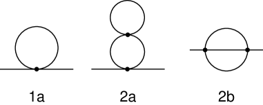
FIG. 2.: One-loop and two-loop diagrams that contribute to the self-energy.

The one-loop self-energy $\Pi_{1}$, which is independent of $P^{2}$, can be written

$$\Pi_{1}\;=\;\Pi_{\rm 1a}+\Delta_{1}m^{2}\,.$$ (88)

The expression for the one-loop diagram 1a in Fig. 2 is

$$\Pi_{\rm 1a}\;=\;{1\over 2}\bar{g}^{2}I_{1}\,,$$ (89)

where the one-loop integral $I_{1}$ is given in (A.12). Adding the counterterm in (72), the one-loop self energy is

$$\Pi_{1}\;=\;-{1\over 2}(\bar{L}+1)\bar{\alpha}\,\bar{m}^{2}\,.$$ (90)

The two-loop self-energy function, which depends on $P^{2}$, is

$$\Pi_{2}(P^{2}) = \Pi_{\rm 2a}+\Pi_{\rm 2b}(P^{2})+{\partial\Pi_{\rm 1a}\over\partial\bar{m}^{2}}\Delta_{1}m^{2}+{\Pi_{\rm 1a}\over\bar{g}^{2}}\Delta_{1}g^{2}+\Delta_{2}m^{2}\,.$$ (91)

The expressions for the two-loop diagrams 2a and 2b in Fig. 2 are

$$\Pi_{\rm 2a} = -{1\over 4}\bar{g}^{4}I_{1}I_{2}\,,$$ (92)

$$\Pi_{\rm 2b}(P^{2}) = -{1\over 6}\bar{g}^{4}I_{\rm sun}(P^{2})\,.$$ (93)

To calculate the physical mass to order $\bar{\alpha}^{2}$, we need the value of $\Pi_{\rm 2a}(P^{2})$ only at $P^{2}=-\bar{m}^{2}$. Inserting the values for $I_{1}$ and $I_{2}$ from the Appendix and the value of $I_{\rm sun}(-\bar{m}^{2})$ from (35), we obtain

$$\Pi_{\rm 2a} = {\bar{\alpha}^{2}\over 4}\left({\mu\over\bar{m}}\right)^{4\epsilon}\left[{1\over\epsilon^{2}}+{1\over\epsilon}+1+{\pi^{2}\over 6}\right]\bar{m}^{2}\,,$$ (94)

$$\Pi_{\rm 2b}(-\bar{m}^{2}) = {\bar{\alpha}^{2}\over 4}\left({\mu\over\bar{m}}\right)^{4\epsilon}\left[{1\over\epsilon^{2}}+{17\over 6\epsilon}-{2\over 3}C_{1}\right]\bar{m}^{2}\,.$$ (95)

Combining all of the terms in (91), the value of the two-loop self-energy at $P^{2}=-\bar{m}^{2}$ is

$$\Pi_{2}(-\bar{m}^{2}) = \left[{1\over 2}\bar{L}^{2}+{7\over 6}\bar{L}-{1\over 2}-{\pi^{2}\over 24}-{1\over 6}C_{1}\right]\bar{\alpha}^{2}\,\bar{m}^{2}\,.$$ (96)

The solution to the equation (87) for $m^{2}$ to order $\bar{\alpha}^{2}$ is

$$m^{2}\;=\;\bar{m}^{2}+\Pi_{1}+\Pi_{2}(-\bar{m}^{2})\,.$$ (97)

Inserting (90) and (96) into (97), our final result for the physical mass to order $\bar{\alpha}^{2}$ is

$$m^{2}\;=\;\left[1-{1\over 2}(\bar{L}+1)\bar{\alpha}+\left({1\over 2}\bar{L}^{2}+{7\over 6}\bar{L}-{1\over 2}-{\pi^{2}\over 24}-{1\over 6}C_{1}\right)\bar{\alpha}^{2}\right]\bar{m}^{2}.$$ (98)

B Physical coupling constant

A convenient physical definition of the coupling constant $g$ is that the amplitude for $2\to 2$ scattering is exactly $-g^{2}$ at threshold where all four particles have four-momentum $p=(m,0)$. To express the free energy in terms of $g$ to three-loop order, we need to calculate $g^{2}$ to order $\bar{g}^{4}$.

The one-loop expression for the negative of the scattering amplitude at threshold is

$$g^{2}\;=\;\bar{g}^{2}-{1\over 2}\bar{g}^{4}\left[I_{\rm bubble}(-4m^{2})+2\,I_{\rm bubble}(0)\right]+\Delta_{1}g^{2}.$$ (99)

where the bubble integral is defined in (37). Using the result (38), the values of the bubble integrals that appear in (99) are

$$I_{\rm bubble}(-4m^{2}) = {1\over(4\pi)^{2}}\left({\mu\over\bar{m}}\right)^{2\epsilon}\left[{1\over\epsilon}+2\right]\,,$$ (100)

$$I_{\rm bubble}(0) = {1\over(4\pi)^{2}}\left({\mu\over\bar{m}}\right)^{2\epsilon}{1\over\epsilon}\,.$$ (101)

We have neglected the difference between $m$ and $\bar{m}$ in the bubble integrals because it is higher order in $\bar{\alpha}$. Inserting (100) and (101) together with (82) into (99), our final result for the physical coupling constant $\alpha=g^{2}/(4\pi)^{2}$ is

$$\alpha\;=\;\left[1-\left({3\over 2}\bar{L}+1\right)\bar{\alpha}\right]\bar{\alpha}\,.$$ (102)

C Three-loop free energy

To express the three-loop free energy in terms of the physical mass and coupling constant, we need to invert (98) and (102) to obtain $\bar{m}^{2}$ and $\bar{g}^{2}$ in terms of $m^{2}$ and $g^{2}$, insert them into our expression for the free energy, and expand to order $\alpha^{2}$. Inverting (98) and (102), we obtain

$$\bar{m}^{2} = \left[1+{1\over 2}(L+1)\alpha+\left({1\over 2}L^{2}+{1\over 3}L+1+{\pi^{2}\over 24}+{1\over 6}C_{1}\right)\alpha^{2}\right]m^{2}\,,$$ (103)

$$\bar{\alpha} = \left[1+\left({3\over 2}L+1\right)\alpha\right]\alpha\,,$$ (104)

where $L=\log(\mu^{2}/m^{2})$, not to be confused with $\bar{L}=\log(\mu^{2}/\bar{m}^{2})$ in (98) and (102). Upon inserting these expressions into the sum of (67), (73), and (85), and expanding to order $\alpha^{2}$, all the terms that depend on $L$ cancel. Our final expression for the temperature-dependent contribution to the free energy in terms of physical parameters is

$${\cal F} = -{1\over 2(4\pi)^{2}}\left[J_{0}\;-\;{\alpha\over 4}J_{1}^{2}\;+\;{\alpha^{2}\over 8}\left(2J_{1}^{2}+J_{1}^{2}J_{2}+2K_{2}+{4\over 3}K_{3}\right)\right]T^{4}\,,$$ (105)

where $K_{n}$ and $J_{n}$ are the functions of $\beta m$ defined by (46), (58), (68), (74), and (86). This expression is remarkably compact.

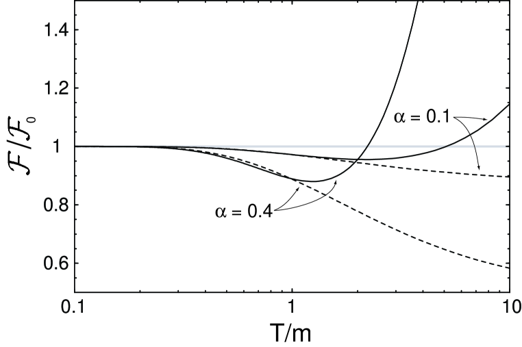
FIG. 3.: Free energy normalized to that of an ideal gas vs. $T/m$ for $\alpha=0.1$ and 0.4. The dashed and solid lines are the two- and three-loop approximations to the free energy, respectively.

The effect of the interaction on the free energy (which is the negative of the pressure) is illustrated in Fig. 3. We normalize the free energy to that of an ideal gas of particles with the same physical mass $m$, which is given by ${\cal F}_{0}$ in (67). We plot ${\cal F}/{\cal F}_{0}$ as a function of $T/m$ on a log scale for two different values of the physical coupling constant: $\alpha=0.1$ and $\alpha=0.4$, which correspond to $g=3.97$ and $g=7.95$, respectively. The dashed lines are the free energies truncated after the order-$\alpha$ terms. The solid lines are the free energies truncated after the order-$\alpha^{2}$ terms.

For $T\ll m$, the three-loop result for the free energy (105) approaches

$${\cal F} \longrightarrow {\cal F}_{0}\left\{1\;-\;{\alpha-2\alpha^{2}\over 2}\left({2\pi T\over m}\right)^{1/2}e^{-m/T}\right\}\,.$$ (106)

The exponential approach to the free energy of an ideal gas is evident in Fig. 3. Note that the order-$\alpha^{2}$ correction is smaller than the order-$\alpha$ correction only if $\alpha<\mbox{${1\over 2}$}$. For $T\gg m$, (105) approaches

$${\cal F} \longrightarrow {\cal F}_{0}\left\{1\;-\;{5\over 4}\alpha\;+\;\left[{5\pi\over 4}{T\over m}-{15\over 4}\log{T\over m}-6.6245\right]\alpha^{2}\right\}\,.$$ (107)

In the order-$\alpha^{2}$ correction, the linearly divergent $T/m$ term is the first of a series of infrared divergent terms that behave like $\alpha^{n+1}(T/m)^{2n-1}$. These terms come from the ring diagrams which, when summed to all orders, give a correction of $+(5\sqrt{6}/3)\alpha^{3/2}$. The logarithm in the order-$\alpha^{2}$ correction term arises from the running of the coupling constant. It can be absorbed into the order-$\alpha$ correction term by replacing the physical coupling constant $\alpha$ by $\bar{\alpha}(T)$, the $\overline{MS}$ coupling constant with renormalization scale $\mu=T$. For $T\gg m$, we expect the three-loop result to be a good approximation only if the $\alpha^{2}T/m$ correction is small compared to the $\alpha$ correction, which requires $T\ll m/(\pi\alpha)$.

V Summary

We have reduced the thermal basketball diagram for a massive scalar field theory with a $\phi^{4}$ interaction to three-dimensional integrals that can be evaluated numerically. As an application, we calculated the free energy for this theory to order $\alpha^{2}$. The result is particularly simple if the free energy is expressed in terms of the physical mass and coupling constant. Another useful application of our result for the massive thermal basketball diagram would be to extend the calculation of the free energy for the massless theory using screened perturbation theory to three-loop accuracy [16].

A One-loop Sum-integrals

The one-loop sum-integrals required to calculate the free energy to order $g^{4}$ are

$${\cal I}_{0}^{\prime} = -\hbox{$\sum$}\!\!\!\!\!\!\int_{P}\log\left(P^{2}+m^{2}\right)\,,$$ (A.1)

$${\cal I}_{n} = \hbox{$\sum$}\!\!\!\!\!\!\int_{P}{1\over(P^{2}+m^{2})^{n}}\,.$$ (A.2)

The sum-integral ${\cal I}_{0}^{\prime}$ is the derivative of ${\cal I}_{n}$ with respect to its index evaluated at $n=0$. These integrals satisfy

$${\partial\ \ \over\partial m^{2}}{\cal I}_{0}^{\prime} = -{\cal I}_{1}\,,$$ (A.3)

$${\partial\ \ \over\partial m^{2}}{\cal I}_{n} = -n{\cal I}_{n+1}\,.$$ (A.4)

The specific sum-integrals that are required are ${\cal I}_{0}^{\prime}$, ${\cal I}_{1}$, and ${\cal I}_{2}$. The temperature-dependent terms in the sum-integrals can be conveniently expressed in terms of the following integrals:

$$J_{n}\;=\;{4e^{\gamma\epsilon}\Gamma({1\over 2})\over\Gamma({5\over 2}-n-\epsilon)}{m^{2\epsilon}\over T^{4-2n}}\int_{0}^{\infty}dp\;{p^{4-2n-2\epsilon}\over E_{p}}n(E_{p})\;.$$ (A.5)

These integrals are functions of $\beta m$ only and satisfy the recursion relation

$$m{\partial\ \over\partial m}J_{n}\;=\;2\epsilon J_{n}-2(\beta m)^{2}J_{n+1}\;.$$ (A.6)

If we separate out the temperature-dependent terms in the one-loop sum-integrals, the resulting expressions are

$${\cal I}_{0}^{\prime} = {1\over(4\pi)^{2}}\left({\mu\over m}\right)^{2\epsilon}\left[{e^{\gamma\epsilon}\Gamma(1+\epsilon)\over\epsilon(1-\epsilon)(2-\epsilon)}m^{4}+J_{0}T^{4}\right]\;,$$ (A.7)

$${\cal I}_{1} = {1\over(4\pi)^{2}}\left({\mu\over m}\right)^{2\epsilon}\left[-{e^{\gamma\epsilon}\Gamma(1+\epsilon)\over\epsilon(1-\epsilon)}m^{2}+J_{1}T^{2}\right]\;,$$ (A.8)

$${\cal I}_{2} = {1\over(4\pi)^{2}}\left({\mu\over m}\right)^{2\epsilon}\left[{e^{\gamma\epsilon}\Gamma(1+\epsilon)\over\epsilon}+J_{2}\right]\;.$$ (A.9)

To calculate the physical mass and coupling constant, we also need the one-loop Euclidean momentum integrals $I_{1}$ and $I_{2}$ defined by

$$I_{n}\;=\;\int_{P}{1\over(P^{2}+m^{2})^{n}}\;.$$ (A.10)

These integrals satisfy

$${\partial\ \ \over\partial m^{2}}I_{n}\;=\;-nI_{n+1}\;.$$ (A.11)

The integrals $I_{1}$ and $I_{2}$ are identical to the temperature-independent terms in (A.8) and (A.9), respectively. Expanding around $\epsilon=0$, these integrals are

$$I_{1} = {1\over(4\pi)^{2}}\left({\mu\over m}\right)^{2\epsilon}\left[-{1\over\epsilon}-1-\left(1+{\pi^{2}\over 12}\right)\epsilon+O(\epsilon^{2})\right]m^{2}\,,$$ (A.12)

$$I_{2} = {1\over(4\pi)^{2}}\left({\mu\over m}\right)^{2\epsilon}\left[{1\over\epsilon}+{\pi^{2}\over 12}\epsilon+O(\epsilon^{2})\right]\,.$$ (A.13)

Addendum

After this paper was completed, J.-M. Chung [17] provided us with analytic expressions for the coefficients $C_{0}$ and $C_{1}$ defined in (23) and (35):

$$C_{0} = {275\over 12}+{23\over 2}\,\zeta(2)-2\,\zeta(3)\,,$$ (A.14)

$$C_{1} = -{59\over 8}-{3\over 2}\,\zeta(2)\,.$$ (A.15)

These analytic expressions can be derived using the methods described in Refs. [18, 19].

REFERENCES

• [1] E. Braaten and R.D. Pisarski, Phys. Rev. Lett. 64, 1338 (1990); Nucl. Phys. B337, 569 (1990).
• [2] E. Braaten and R.D. Pisarski, Phys. Rev. D42, 2156 (1990).
• [3] J. Frenkel, A.V. Saa, and J.C. Taylor, Phys. Rev. D46, 3670 (1992).
• [4] C. Corianò and R.R. Parwani, Phys. Rev. Lett. 73, 2398 (1994).
• [5] P. Arnold and C. Zhai, Phys. Rev. D50, 7603 (1994); Phys. Rev. D51, 1906 (1995).
• [6] R.R. Parwani and H. Singh, Phys. Rev. D51, 4518 (1995).
• [7] E. Braaten and A. Nieto, Phys. Rev. D51, 6990 (1995).
• [8] R.R. Parwani, Phys. Lett. B334, 420 (1994); R.R. Parwani and C. Corianò, Nucl. Phys. B434, 56 (1995).
• [9] J.O. Andersen, Phys. Rev. D53, 7286 (1996).
• [10] B. Kastening and C. Zhai, Phys. Rev. D52, 7232 (1995).
• [11] E. Braaten and A. Nieto, Phys. Rev. Lett. 76, 1417 (1996); Phys. Rev. D53, 3421 (1996).
• [12] F. Karsch, A. Patkós, and P. Petreczky, Phys. Lett. B401, 69 (1997).
• [13] A.I. Bugrij and V.N. Shadura, hep-th/9510232.
• [14] B. Kastening, Phys. Rev. D54, 3965 (1996).
• [15] J.-M. Chung and B.K. Chung, Phys. Rev. D56, 6508 (1997).
• [16] J.O. Andersen, E. Braaten, and M. Strickland (in progress).
• [17] J.-M. Chung, private communication.
• [18] S. Groote, J.G. Körner and A.A. Pivovarov, Phys. Lett. B443, 269 (1998); Nucl. Phys. B542, 515 (1999); Eur. Phys. J. C11, 279 (1999).
• [19] F.A. Berends, A.I. Davydychev, and N.I. Ussyukina, Phys. Lett. B426, 95 (1998); J.-M. Chung and B.K. Chung, hep-th/9911196.