hep-ph/0002032 FERMILAB-Pub-00/032-T CTEQ-015 MSUHEP-00126 UH-511-954-00
Higgs Production:
A Comparison of Parton Showers and Resummation

Abstract

The search for the Higgs boson(s) is one of the major priorities at the upgraded Fermilab Tevatron and at the CERN Large Hadron Collider (LHC). Monte Carlo event generators (MCs) are heavily utilized to extract and interpret the Higgs signal, which depends on the details of the soft–gluon emission from the initial state partons in hadronic collisions. Thus, it is crucial to establish the reliability of the MCs used by the experimentalists. In this paper, the MC based parton shower formalism is compared to that of an analytic resummation calculation. Theoretical input, predictions and, where they exist, data for the transverse momentum distribution of Higgs bosons, $Z^{0}$ bosons, and photon pairs are compared for the Tevatron and the LHC. This comparison is useful in understanding the strengths and the weaknesses of the different theoretical approaches, and in testing their reliability.

I Introduction

To reveal the dynamics of the electroweak symmetry breaking, a new generation of hadron colliders will search for the Higgs boson(s). The potential of the upgraded Fermilab Tevatron, the 2 TeV center of mass energy proton-antiproton collider starting operation within a year, was analysed in Ref. [1]. Later in this decade, two experimental collaborations (ATLAS and CMS) join the search at the CERN Large Hadron Collider (LHC) with 14 TeV proton-proton collisions. An extraction of the Higgs signal at the LHC requires not only the precise knowledge of the signal and background invariant mass distributions, but also the accurate prediction of the corresponding transverse momentum ($p_{T}$) distributions. In general, the determination of the signal requires a detailed event modeling, an understanding of the detector resolution, kinematical acceptance and efficiency, all of which depend on the $p_{T}$ distribution. The shape of this distribution in the low to moderate $p_{T}$ region, can dictate the details of both the experimental triggering and the analysis strategies for the Higgs search. It can also be used to devise an improved search strategy, and to enhance the statistical significance of the signal over the background [2, 3]. In the $gg\to HX\to\gamma\gamma X$ mode at the LHC, for example, the shape of the signal and the background $p_{T}$ distribution of the photon pairs is different (c.f. Refs. [4, 5]), with the signal being harder. This difference can be utilized to increase the signal to background ratio. Furthermore, since vertex pointing with the photons is not possible in the CMS barrel, the shape of the $p_{T}$ distribution affects the precision of the determination of the event vertex from which the Higgs (decaying into two photons) originated.  Thus, for a successful, high precision extraction of the Higgs signal, the theoretical calculation must be capable of reproducing the expected transverse momentum distribution.

To reliably predict the $p_{T}$ distribution of Higgs bosons at the LHC, especially for the low to medium $p_{T}$ region where the bulk of the rate is, the effects of the multiple soft–gluon emission have to be included. One approach which achieves this is parton showering [6]. Parton shower Monte Carlo programs such as PYTHIA[7], HERWIG[8] and ISAJET[9] are commonly used by experimentalists, both as a way of comparing experimental data to theoretical predictions, and also as a means of simulating experimental signatures in kinematic regimes for which there are no experimental data yet (such as for the LHC). The final output of these Monte Carlo programs consists of the 4-momenta of a set of final state particles. This output can either be compared to reconstructed experimental quantities or, when coupled with a simulation of a detector response, can be directly compared to raw data taken by the experiment, and/or passed through the same reconstruction procedures as the raw data. In this way, the parton shower programs can be more useful to experimentalists than analytic calculations. Indeed, almost all of the physics plots in the ATLAS physics TDR [10] involve comparisons to PYTHIA version 5.7.

Predictions of the Higgs $p_{T}$ can also be obtained utilizing an analytic resummation formalism, which sums contributions of $\alpha_{S}^{n}\ln^{m}(m_{H}/p_{T})$ (where $m_{H}$ is the Higgs mass, and $m\leq 2n-1$) up to all orders in the strong coupling $\alpha_{S}$. In the recent literature, most calculations of this kind are either based on, or originate from, the low $p_{T}$ factorization formalism[11] (for the latest review see Ref. [12]). This formalism resums the effects of the multiple soft–gluon emission while also systematically including the fixed order QCD corrections. It is possible to smoothly match the resummed result to the fixed order one in the intermediate to high $p_{T}$ region, thus obtaining a prediction for the full $p_{T}$ distribution [13]. In this paper, we use this formalism as the analytic ‘benchmark’ to calculate the $p_{T}$ distributions of Higgs bosons at the LHC, and of $Z^{0}$ bosons and photon pairs produced in hadron collisions.

For many physical quantities, the predictions from parton shower Monte Carlo programs should be nearly as precise as those from analytic theoretical calculations. It is expected that both the Monte Carlo and analytic calculations should accurately describe the effects of the emission of multiple soft–gluons from the incoming partons, an all orders problem in QCD. The initial state soft–gluon emission affects the kinematics of the final state partons. This may have an impact on the signatures of physics processes at both the trigger and analysis levels and thus it is important to understand the reliability of such predictions. The best method for testing the reliability is a direct comparison of the predictions to experimental data. If no experimental data are available for certain predictions, then some understanding of the reliability may be gained from the comparison of the predictions from the two different methods.

In the absence of experimental data for Higgs production, we can gauge the reliability of calculations for this process by comparing them to each other. We also compare predictions form the different formalisms to data for processes which are similar to Higgs production at the LHC. In this way we can perform a genuine ‘reality check’ of the various theoretical predictions. Production of a light, neutral Higgs boson at the LHC in the standard model (SM) and its supersymmetric extensions proceeds via the partonic subprocess $gg$ (through heavy fermion loop) $\to HX$. One of the major backgrounds for a light Higgs, in the mass range of 100 GeV $\lesssim m_{H}\lesssim$ 150 GeV, is diphoton production, a sizable contribution to which comes from the same, $gg$ initial state. Since the major part of the soft–gluon radiation is initiated from the incoming partons, the structures of the resummed corrections are similar for Higgs boson and diphoton production. Because the latter is measurable at the Fermilab Tevatron, diphoton production provides an exceptional opportunity to test the different theoretical models. $Z^{0}$ boson production can also be a good testing ground for the soft–gluon corrections to Higgs production. The treatment of the fixed order and resummed QCD corrections for $Z^{0}$ boson production is theoretically well understood and implemented at next-to-next-to-leading order [13]. Furthermore, just as in the diphoton case, predictions can also be tested against Tevatron data. The $Z^{0}$ data have the advantage that sufficient statistics exist in the Run 1 data from CDF and D0 to allow for detailed comparisons to the theoretical predictions.

II Low $p_{T}$ Factorization

In this section the low transverse momentum factorization formalism and its matching to the usual factorization is reviewed. The problem arises as follows. When calculating fixed order QCD corrections to the $p_{T}$ distribution of the inclusive process $pp\to HX$, the standard QCD factorization theorem is invoked

$$\frac{d\sigma}{dp_{T}^{2}}=f_{j_{1}/p}(m_{H})\otimes\frac{d{\hat{\sigma}}_{j_{1}j_{2}}}{dp_{T}^{2}}(m_{H},p_{T})\otimes f_{j_{2}/p}(m_{H}),$$ (1)

which is a convolution in the partonic momentum fractions, and is derived under the usual assumption $p_{T}\gg m_{H}$.  When $p_{T}\ll m_{H}$ occurs, as a result of soft and soft+collinear emission of gluons from the initial state, the theorem fails. The ratio of the two very different physical scales in the partonic cross section ${\hat{\sigma}}_{j_{1}j_{2}}$, produces large logarithms of the form $\ln(m_{H}/p_{T})$, which are not absorbed by the parton distribution functions $f_{j/p}$, unlike the ones originating from purely collinear parton emission. These logs are enhanced by a $1/p_{T}^{2}$ pre-factor at low $p_{T}$. (The same factor suppresses them for large $p_{T}$.) As a result, the Higgs $p_{T}$ distribution calculated using the conventional hadronic factorization theorem is un-physical in the low $p_{T}$ region.

To resolve this problem, the differential cross section is split into a part which contains all the logarithmic terms ($W$), and into a regular term ($Y$):

$$\frac{d\sigma}{dp_{T}^{2}}=W(m_{H},p_{T})+Y(m_{H},p_{T}),$$ (2)

Since $Y$ does not contain logs of $p_{T}$, it can be calculated using the usual factorization. The $W$ term has to be evaluated differently, keeping in mind that failure of the standard factorization occurs because it neglects the transverse motion of the incoming partons in the hard scattering. As has been proven [11], $W$ has a simple form in the Fourier conjugate, that is the transverse position (${\vec{b}}$) space

$$\widetilde{W}(m_{H},b)={\cal C}_{j_{1}/h_{1}}(m_{H},b)\,e^{-{\cal S}(m_{H},b_{*})}\,{\cal C}_{j_{2}/h_{2}}(m_{H},b),$$ (3)

with the Sudakov exponent defined as

$${\cal S}(m_{H},b_{*})=\int_{C_{0}^{2}/b_{*}^{2}}^{m_{H}^{2}}\frac{d\mu^{2}}{\mu^{2}}\left[A\left(\alpha_{S}(\mu)\right)\ln\left(\frac{m_{H}^{2}}{\mu^{2}}\right)+B\left(\alpha_{S}(\mu)\right)\right],$$ (4)

which resums the large logarithmic terms.  The partonic recoil against soft gluons, as well as the intrinsic partonic transverse momentum, are included in the generalized parton distributions

$${\cal C}_{j/h}(m_{H},b,x)=\left[C_{ja}\left(m_{H},b_{*}\right)\otimes f_{a/h}(m_{H})\right](x)\;{\cal F}_{a/h}(m_{H},b,x),$$ (5)

where the convolution is evaluated over the partonic momentum fraction $x$. The $A$ and $B$ functions, and the Wilson coefficients $C_{ja}$ are free of logs and safely calculable perturbatively as expansions in the strong coupling

$$A(\alpha_{S})=\sum_{n=1}^{\infty}\left(\frac{\alpha_{S}}{\pi}\right)^{n}A^{(n)},~{}~{}~{}{\rm etc.}$$ (6)

The process independent non-perturbative functions ${\cal F}_{a/h}$, describing long distance transverse physics, are extracted from low-energy experiments [14].

The matching of the low and the high $p_{T}$ regions is achieved via the $Y$ piece. To correct the behavior of the resummed piece in the intermediate and high $p_{T}$ regions, it is defined as the difference of the cross section calculated by the standard factorization formula at a fixed order $n$ of perturbation theory and its $p_{T}\ll m_{H}$ asymptote.  The resummed cross section, to order $\alpha_{S}^{n}$, then reads as

$$\frac{d\sigma}{dp_{T}^{2}}=W(m_{H},p_{T})+\frac{d\sigma^{(n)}}{dp_{T}^{2}}-\left.\frac{d\sigma^{(n)}}{dp_{T}^{2}}\right|_{p_{T}\ll m_{H}}$$ (7)

At low $p_{T}$, the logarithms are large and the asymptotic part dominates the fixed order $p_{T}$ distribution. The last two terms in Eq. (7) nearly cancel, and $W$ is a good approximation to the cross section. At high $p_{T}$ the logarithms are small, and the expansion of the resummed term cancels the $p_{T}$ singular terms (up to higher orders in $\alpha_{S}$), and the cross section reduces to the fixed order perturbative result. After matching the resummed and fixed order cross sections in such a manner, it is expected that the normalization of the resummed cross section reproduces the fixed order total rate, since when expanded and integrated over $p_{T}$ it deviates from the fixed order result only in higher order terms. For further details of the low $p_{T}$ factorization formalism and its application to Higgs production we refer to the recent literature [5, 16].

III Parton Showering and Resummation

For technical reasons, the initial state parton shower proceeds by a $\it{backwards}$ evolution, starting at the large (negative) $Q^{2}$ scale of the hard scatter and then considering emissions at lower and lower (negative) virtualities, corresponding to earlier points on the cascade (and earlier points in time), until a scale corresponding to the factorization scale is reached. The transverse momentum of the initial state is built up from the whole series of splittings and boosts. The showering process is independent of the hard scattering process being considered (as long as one does not introduce any matrix element corrections), and depends only on the initial state partons and the hard scale of the process.

Parton showering utilizes the fact that the leading order singularities of cross sections factorize in the collinear limit. This is expressed as

$$\lim_{p_{b}||p_{g}}|{\cal M}_{n+1}|^{2}=\frac{2\pi\alpha_{S}}{p_{b}.p_{g}}P_{a\to bg}(z)|{\cal M}_{n}|^{2},$$ (8)

where ${\cal M}_{n+1}$ is the invariant amplitude for the process producing $n$ partons and a gluon, $\alpha_{S}$ is the strong coupling constant, $p_{b}$ and $p_{g}$ are the 4-momenta of the daughters of parton $a$, and $P_{a\to bg}(z)$ is the DGLAP evolution kernel associated with the $a\to bg$ splitting. These leading order collinear singularities can be factorized into a Sudakov form factor

$${\cal S}_{\rm shower}(Q)=\int_{Q_{0}^{2}}^{Q^{2}}\frac{d\mu^{2}}{\mu^{2}}\frac{\alpha_{S}(\mu)}{2\pi}\int_{0}^{1}dz\,P_{a\to bg}(z),$$ (9)

which is interpreted as the probability ${\cal P}=\exp(-{\cal S}_{\rm shower})$ of the partonic evolution from scale $Q_{0}$ to $Q$ with no resolvable branchings. This probability can be used to determine the scale for the first emission and hence for the whole cascade. The formalism can be extended to soft singularities as well by using angular ordering. In this approach, the choice of the hard scattering is based on the use of evolved parton distributions, which means that the inclusive effects of initial-state radiation are already included. What remains is, therefore, to construct the exclusive showers.

Parton showering resums primarily the leading logs which are universal, that is process independent and depend only on the given initial state. In this lies one of the strengths of Monte Carlos, since parton showering can be incorporated into a wide variety of physical processes. An analytic calculation, in comparison, can resum all logs. For example, the low $p_{T}$ factorization formalism sums all of the logarithms with $m_{H}/p_{T}$ in their arguments. As discussed earlier, all of the ‘dangerous logs’ are included in the Sudakov exponent (4). The $A$ and $B$ functions in Eq.(4) contain an infinite number of coefficients, with the $A^{(n)}$ coefficients being universal, while the $B^{(n)}$’s are process dependent, with the exception of $B^{(1)}$. In practice, the number of towers of logarithms included in the analytic Sudakov exponent depends on the level to which a fixed order calculation was performed for a given process. Generally, if a next-to-next-to-leading order calculation is available, then $B^{(2)}$ can be extracted and incorporated. Extraction of higher coefficients require the knowledge of even higher order QCD corrections. So far, only the $A^{(1)}$, $A^{(2)}$ and $B^{(1)}$ coefficients are known for Higgs production but the calculation of $B^{(2)}$ is in progress [17]. If we try to interpret parton showering in the same language then we can say that the Monte Carlo Sudakov exponent always contains a term analogous to $A^{(1)}$. It was shown in Ref. [18] that a term equivalent to $B^{(1)}$ is also included in the (HERWIG) shower algorithm, and a suitable modification of the Altarelli-Parisi splitting function, or equivalently the strong coupling constant $\alpha_{S}$, also effectively approximates the $A^{(2)}$ coefficient. 

In contrast with the shower Monte Carlos, analytic resummation calculations integrate over the kinematics of the soft–gluon emission, with the result that they are limited in their predictive power to inclusive final states. While the Monte Carlo maintains an exact treatment of the branching kinematics, in the original low $p_{T}$ factorization formalism no kinematic penalty is paid for the emission of the soft–gluons, although an approximate treatment of this can be incorporated into its numerical implementations, such as ResBos [5, 13]. Neither the parton showering process nor the analytic resummation translate smoothly into kinematic configurations where one hard parton is emitted at large $p_{T}$. In the Monte Carlo matrix element corrections, and in the analytic resummation calculation matching, is necessary. This matching is standard procedure for resummed calculations, and matrix element corrections are becoming increasingly common in Monte Carlos [19, 20, 21].

With the appropriate input from higher order cross sections, a resummation calculation has the corresponding higher order normalization and scale dependence. The normalization and scale dependence for the Monte Carlo, though, remains that of a leading order calculation. The parton showering process redistributes the events in phase space, but does not change the total cross section (for example, for the production of a Higgs boson). 

One quantity which is expected to be well described by both calculations is the transverse momentum of the final state electroweak boson in a subprocess such as $q\overline{q}\to W^{\pm}X$, $Z^{0}X$ or $gg\to HX$, where most of the $p_{T}$ is provided by initial state parton emission. The parton showering supplies the same sort of transverse kick as the resummed soft–gluon emission in the analytic calculation. Indeed, similar Sudakov form factors appear in both approaches. The correspondence between the Sudakov form factors of resummation and Monte Carlo approaches embodies many subtleties, relating to both the arguments of the Sudakov factors as well as the impact of sub-leading logs [22].

At a point in its evolution, typically corresponding to the virtuality of a few GeV², the parton shower is cut off and the effects of gluon emission at softer scales must be parameterized and inserted by hand. This is similar to the somewhat arbitrary division between perturbative and non-perturbative regions in the resummation calculation. The parameterization is typically expressed in a Gaussian form, similar to that used for the non-perturbative $k_{T}$ in a resummation program [14]. In general, the value for the non-perturbative $\langle k_{T}\rangle$ needed in a Monte Carlo program will depend on the particular kinematics and initial state being investigated. A value of the average non-perturbative $k_{T}$ of greater than 1 GeV, for example, does not imply that there is an anomalous intrinsic $k_{T}$ associated with the parton size. Rather, this amount of $\langle k_{T}\rangle$ needs to be supplied to provide what is missing in the truncated parton shower. If the shower is cut off at a higher virtuality, more of the ‘non-perturbative’ $k_{T}$ will be needed.

IV $Z^{0}$ Boson Production at the Tevatron

From a theoretical viewpoint, $Z^{0}$ production at the Tevatron is one of the highest precision testing grounds for the effects of multiple soft-gluon emission. The fully differential fixed order cross section has been calculated up to ${\cal O}(\alpha_{S}^{2})$, and the $A^{(1,2)}$, $B^{(1,2)}$, and $C^{(1)}$ resummed coefficients are known for this process, and have been numerically implemented [13]. Since the ${\cal O}(\alpha_{S}^{2})$ corrections are relatively small (the order of a percent), the contribution of $B^{(2)}$ is almost negligible. Thus, nominally the same perturbative physics is implemented in the shower Monte Carlos as in the resummation calculation. Any differences between their predictions can be ascribed to the small differences in the implementation of the perturbative physics, and to the different non-perturbative physics they contain. Experimentally, the 4-momentum of a $Z^{0}$ boson, and thus its $p_{T}$, can be measured with great precision in the $e^{+}e^{-}$ decay mode. Resolution effects are relatively minor and are easily corrected. Thus, the $Z^{0}$ $p_{T}$ distribution is an excellent probe of the effects of the soft–gluon emission.

The resolution corrected $p_{T}$ distribution (in the low $p_{T}$ region) for $Z^{0}$ bosons from the CDF experiment [23] is shown in Figure 1, compared to both the resummed prediction of ResBos, and to two predictions from PYTHIA version 6.125. One PYTHIA prediction uses the default value of intrinsic $k_{T}^{\rm rms}=0.44$ GeV (dashed histogram), and the second a value of 2.15 GeV (solid histogram), per incoming parton.  The latter value was found to give the best agreement for PYTHIA with the data, and a similar conclusion has been reached in comparisons of the CDF $Z^{0}$ $p_{T}$ data with HERWIG [24]. All of the predictions use the CTEQ4M parton distributions [25]. The shift between the two PYTHIA predictions at low $p_{T}$ is clearly evident. As might have been expected, the high $p_{T}$ region (above 10 GeV) is unaffected by the value of the non-perturbative $k_{T}$. Much of the $k_{T}$ ‘given’ to the incoming partons at their lowest virtuality, $Q_{0}$, is reduced at the hard scatter due to the number of gluon branchings preceding the collision. The emitted gluons carry off a sizable fraction of the original non-perturbative $k_{T}$ [26]. This point will be investigated in more detail later for the case of Higgs production.

FIG. 1.: The $Z^{0}$ $p_{T}$ distribution (at low $p_{T}$) from CDF for Run 1 compared to predictions from ResBos (curve) and from PYTHIA (histograms). The two PYTHIA predictions use the default (rms) value for the non-perturbative $k_{T}$ (0.44 GeV) and the value that gives the best agreement with the shape of the data (2.15 GeV). The normalization of the resummed prediction was rescaled upwards by 8.4%. The PYTHIA prediction was rescaled by a factor of 1.4 for the shape comparison. (Including only soft–gluon QCD corrections, PYTHIA does not contain the QCD $K$-factor.)

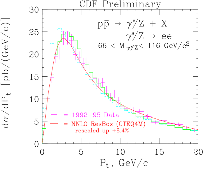
In the resummed calculation it has been shown that, in addition to the perturbative physics (Sudakov and Wilson coefficients, $C_{ja}$), the choice of the non-perturbative parameters affects the shape of the distribution in the lowest $p_{T}$ region and the location of the peak [13]. In order to qualitatively compare this effect to the smearing applied in the Monte Carlos, it is possible to bring the resummation formula to a form where the non-perturbative function acts as a Gaussian type smearing term. This, using the Ladinsky-Yuan parameterization [27] of the non-perturbative function, leads to an rms value of 2.5 GeV for the effective $k_{T}$ smearing parameter, for $Z^{0}$ production at the Tevatron. This is in agreement with the PYTHIA and HERWIG results: to well describe the $Z^{0}$ production data at the Tevatron, 2-2.5 GeV non-perturbative $k_{T}$ is needed in these implementations. The resummed curve agrees with the shape of the data well, which is a non-trivial result, since the resummation calculation does not contain any free parameters which are fitted to the $Z^{0}$ $p_{T}$ distribution. Even with the optimal non-perturbative $k_{T}^{\rm rms}=2.15$ GeV, there is slight shape difference between the shower Monte Carlo and the data. This might be partially due to the lack of the $B^{(2)}$ coefficient in the shower Monte Carlos. This is supported by the fact that, if the $B^{(2)}$ coefficient was not included in the resummed prediction, the result would be an increase in the height of the peak and a decrease in the rate between 10 and 20 GeV, leading to a better agreement with the best PYTHIA prediction [12].

FIG. 2.: The $Z^{0}$ $p_{T}$ distribution (for the full range of $p_{T}$) from CDF for Run 1 compared to predictions from ResBos (curve) and from PYTHIA (histogram). The normalization of the resummed prediction was rescaled upwards by 8.4%. The PYTHIA prediction was rescaled by a factor of 1.4 for the shape comparison.

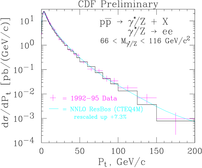
The $Z^{0}$ $p_{T}$ distribution is shown over a wider $p_{T}$ range in Figure 2. The PYTHIA and ResBos predictions both describe the data well. Note especially the agreement of PYTHIA with the data at high $p_{T}$, made possible by explicit matrix element corrections (from the subprocesses $q\overline{q}\to Z^{0}g$ and $gq\to Z^{0}q$) to the $Z^{0}$ production process. 

V Diphoton Production

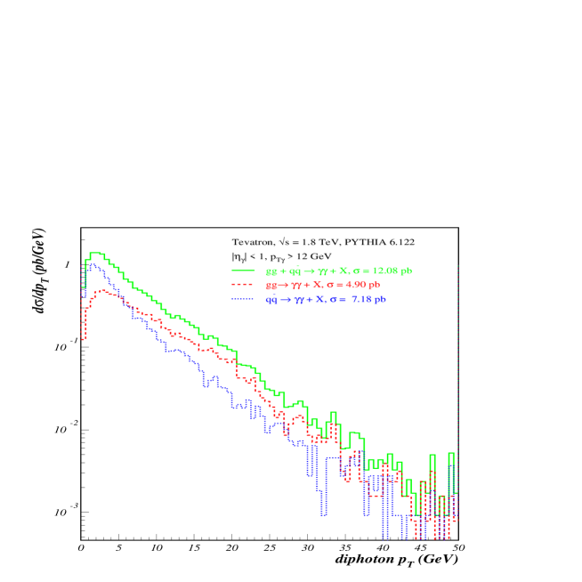
Most of the experience that we have for comparisons of data to resummation calculations or Monte Carlos is based on Drell-Yan pair production, that is mostly on $q\overline{q}$ initial states. It is important then to examine diphoton production at the Tevatron, where a large fraction of the contribution at low mass is due to $gg$ scattering. The prediction for the diphoton $p_{T}$ distribution at the Tevatron, from PYTHIA (version 6.122), is shown in Figure 3, using the experimental cuts applied in the CDF analysis [28]. About half of the diphoton cross section at the Tevatron is due to the $gg$ subprocess, and the diphoton $p_{T}$ distribution is noticeably broader for the $gg$ subprocess than for the $q\overline{q}$ subprocess.

FIG. 3.: A comparison of the PYTHIA predictions for diphoton production at the Tevatron for the two different subprocesses, $q\overline{q}$ and $gg$. The same cuts are applied to PYTHIA as in the CDF diphoton analysis.

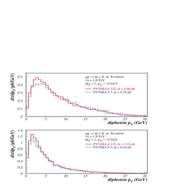
A comparison of the $p_{T}$ distributions for the two diphoton subprocesses $(q\overline{q},gg)$ in two recent versions of PYTHIA, 5.7 and 6.1, is shown in Figure 4. There seems to be little difference in the $p_{T}$ distributions between the two versions for both subprocesses. As will be shown later, this is not true for the case of Higgs production.

FIG. 4.: A comparison of the PYTHIA predictions for diphoton production at the Tevatron for the two different subprocesses, $gg$ (top) and $q\overline{q}$ (bottom), for two recent versions of PYTHIA. The same cuts are applied to PYTHIA as in the CDF diphoton analysis.

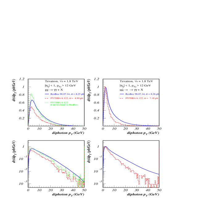
In Figure 5 are shown the ResBos predictions for diphoton production at the Tevatron from $q\overline{q}$ and $gg$ scattering compared to the PYTHIA predictions. The $gg$ subprocess predictions in ResBos agree well with those from PYTHIA while the $q\overline{q}$ $p_{T}$ distribution is noticeably broader in ResBos. The latter behavior is due to the presence of the $Y$ piece in ResBos at moderate $p_{T}$, that is the matching of the $q\overline{q}$ cross section to the fixed order $q\overline{q}\to{\gamma}{\gamma}g$ at high $p_{T}$. The corresponding matrix element correction is not implemented in PYTHIA. The PYTHIA and ResBos predictions for $gg\to{\gamma}{\gamma}$ agree in the moderate $p_{T}$ region, even though the ResBos prediction has the $Y$ piece present and is matched to the matrix element piece $gg\to{\gamma}{\gamma}g$ at high $p_{T}$, while there is no such matrix element correction for PYTHIA. This demonstrates the smallness of the $Y$ piece for the $gg$ subprocess, which is the same conclusion that was reached in Ref. [3]. One way to understand this is recalling that the $gg$ parton-parton luminosity falls very steeply with increasing partonic center of mass energy, $\sqrt{\hat{s}}$. This falloff tends to suppress the size of the $Y$ piece since the production of the diphoton pair at higher $p_{T}$ requires larger values of longitudinal momentum fractions.

FIG. 5.: A comparison of the PYTHIA and ResBos predictions for diphoton production at the Tevatron for the two different subprocesses, $gg$ (left) and $q\overline{q}$ (right). The same cuts are applied to PYTHIA and ResBos as in the CDF diphoton analysis. The bottom figures show the same in logarithmic scale.

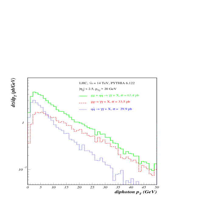
Comparisons of the diphoton data measured by both the CDF [28] and D0 [29] experiments indicate a disagreement of the observed diphoton $p_{T}$ distribution with the NLO QCD predictions [30]. In particular, the $p_{T}$ distribution in the data is noticeably broader than that predicted by fixed order QCD calculations, but in agreement with the predictions of ResBos [31]. The transverse distributions of the diphoton pair are particularly sensitive to the effects of soft–gluon radiation. The $p_{T}$ distribution, for example, is a delta function calculated at leading order, and is strongly smeared by the all order Sudakov factor. Given the small size of the diphoton cross section at the Tevatron, the comparisons for Run 1 are statistically limited. A more precise comparison between theory and experiment will be possible with the 2 $fb^{-1}$ or greater data sample that is expected for CDF and D0 in Run 2, and at the LHC. The Monte Carlo prediction for the diphoton production cross section, as a function of the diphoton $p_{T}$ and using cuts appropriate to ATLAS and CMS, is shown in Figure 6. As at the Tevatron, about half of the cross section is due to $gg$ scattering and the diphoton $p_{T}$ distribution from $gg$ scattering is noticeably broader than that from $q\overline{q}$ production.

FIG. 6.: A comparison of the PYTHIA predictions for diphoton production at the LHC for the two different subprocesses, $q\overline{q}$ and $gg$. Similar cuts are applied to the diphoton kinematics as those used by ATLAS and CMS.

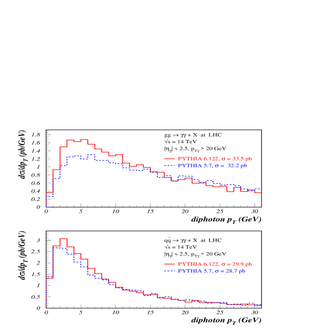
In Figure 7 is shown a comparison of the diphoton $p_{T}$ distribution at the LHC for two different versions of PYTHIA, for the two different subprocesses. Note that the $p_{T}$ distribution in PYTHIA version 5.7 is somewhat broader than that in version 6.122 for the case of $gg$ scattering. The effective diphoton mass range being considered here is lower than the 150 GeV Higgs mass that will be considered in the next section. As will be seen, the differences in soft–gluon emission between the two versions of PYTHIA are larger in that case.

FIG. 7.: A comparison of the PYTHIA predictions for diphoton production at the LHC for the two different subprocesses, $gg$ (top) and $q\overline{q}$ (bottom), for two recent versions of PYTHIA. Similar cuts are applied to the diphoton kinematics as are used by ATLAS and CMS.

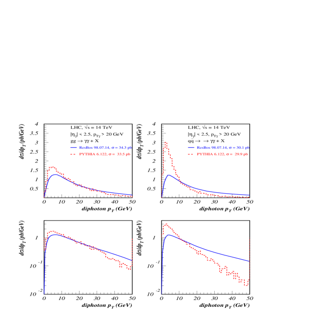
In Figure 8 are shown the ResBos predictions for diphoton production at the LHC from $q\overline{q}$ and $gg$ scattering compared to the PYTHIA predictions. Again, the $gg$ subprocess in ResBos agree well with PYTHIA, while the $q\overline{q}$ $p_{T}$ distribution is noticeably broader in ResBos, for the reasons cited previously.

FIG. 8.: A comparison of the PYTHIA and ResBos predictions for diphoton production at the LHC for the two different subprocesses, $gg$ (left) and $q\overline{q}$ (right). Similar cuts are applied to PYTHIA and ResBos as in the ATLAS and CMS diphoton analyses. The bottom figures show the same in logarithmic scale.

VI Higgs Boson Production

A comparison of the SM Higgs $p_{T}$ distribution at the LHC, for a Higgs mass of 150 GeV, is shown in Figure 9, for ResBos and the two recent versions of PYTHIA. As before, PYTHIA has been rescaled by a factor of 1.7, to agree with the normalization of ResBos to allow for a better shape comparison. There are a number of features of interest. First, the peak of the resummed distribution has moved to $p_{T}\approx$ 11 GeV (compared to about 3 GeV for $Z^{0}$ production at the Tevatron). This is partially due to the larger mass (150 GeV compared to 90 GeV), but is primarily because of the larger color factors associated with initial state gluons ($C_{A}=3$) rather than quarks ($C_{F}=4/3$), and also because of the larger phase space for initial state gluon emission at the LHC.

FIG. 9.: A comparison of predictions for the Higgs $p_{T}$ distribution at the LHC from ResBos and from two recent versions of PYTHIA. The ResBos and PYTHIA predictions have been normalized to the same area. The bottom figure shows the same in logarithmic scale.

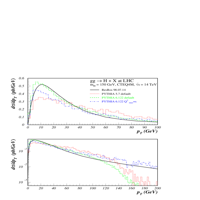
Second, and more importantly, there is a substantial disagreement for the shape of the Higgs $p_{T}$ distribution between ResBos and PYTHIA 5.7, and between the two versions of PYTHIA. An understanding of the reasons for these differences is critical, as the shape of the transverse momentum distribution for the Higgs in the low to moderate $p_{T}$ region, can dictate the details of both the experimental triggering and the analysis strategies for the Higgs search. As noted before, most of the studies for Higgs production by CMS and ATLAS have been based on PYTHIA 5.7. For the CMS detector, the higher $p_{T}$ activity associated with Higgs production in version 5.7 allows for a more precise determination of the event vertex from which the Higgs (decaying into two photons) originates. Vertex pointing with the photons is not possible in the CMS barrel, and the large number of interactions occurring with high intensity running will mean a substantial probability that at least one of the interactions will have more activity than the Higgs vertex, thus leading to the assignment of the Higgs decay to the wrong vertex, and therefore a noticeable degradation of the $\gamma\gamma$ effective mass resolution.

In comparison to ResBos, the older version of PYTHIA produces too many Higgs events at moderate $p_{T}$. Two changes have been implemented in the newer version 6.1. The first change is that a cut is placed on the combination of $z$ (longitudinal momentum fraction) and $Q^{2}$ (partonic virtuality) values in a branching: $\hat{u}=Q^{2}-\hat{s}(1-z)<0$, where $\hat{s}$ refers to the squared invariant mass of the subsystem of the hard scattering plus the shower partons considered to that point. The association with $\hat{u}$ is relevant if the branching is interpreted in terms of a $2\to 2$ hard scattering. The corner of emissions that do not respect this requirement occurs when the $Q^{2}$ value of the space-like emitting parton is little changed and the $z$ value of the branching is close to unity. This effect is mainly for the hardest emission (largest $Q^{2}$). The net result of this requirement is a substantial reduction in the total amount of gluon radiation [32].  In the second change, the parameter for the minimum gluon energy emitted in space-like showers is modified by an extra factor roughly corresponding to the $1/\gamma$ factor for the boost to the hard subprocess frame [32]. The effect of this change is to increase the amount of gluon radiation. Thus, the two effects are in opposite directions but with the first effect being dominant. In principle, this problem could affect the $p_{T}$ distribution for all PYTHIA processes. In practice, it affects only $gg$ initial states, due to the enhanced probability for branching in such an initial state.

The newer version of PYTHIA agrees well with ResBos at low to moderate $p_{T}$, but falls below the resummed prediction at high $p_{T}$. The agreement of the predictions of PYTHIA 6.1 with those of ResBos, in the low to moderate $p_{T}$ region, gives some credence that the changes made in PYTHIA move in the right direction. The disagreement at high $p_{T}$ can be easily understood: ResBos switches to the NLO Higgs+jet matrix element at high $p_{T}$, while the default PYTHIA can generate the Higgs $p_{T}$ distribution only by initial state gluon radiation, using the Higgs mass squared as maximum virtuality. High $p_{T}$ Higgs production is another example where a $2\to 1$ Monte Carlo calculation with parton showering cannot completely reproduce the exact matrix element calculation, without the use of matrix element corrections. The high $p_{T}$ region is better reproduced if the maximum virtuality $Q_{max}^{2}$ is set equal to the squared partonic center of mass energy, $s$, rather than $m_{H}^{2}$. This is equivalent to applying the parton shower to all of phase space. However, this has the consequence of depleting the low $p_{T}$ region, as ‘too much’ showering causes events to migrate out of the peak. The appropriate scale to use in PYTHIA (or any Monte Carlo) depends on the $p_{T}$ range to be probed. If matrix element information is used to constrain the behavior, the correct high $p_{T}$ cross section can be obtained while still using the lower scale for showering. Thus, the incorporation of matrix element corrections to Higgs production (involving the processes $gq\to qH$,$q{\overline{q}}\to gH$, $gg\to gH$) is the next logical project for the Monte Carlo experts, in order to accurately describe the high $p_{T}$ region, and is already in progress [26, 33].

FIG. 10.: A comparison of predictions for the Higgs $p_{T}$ distribution at the Tevatron from ResBos and from two recent versions of PYTHIA. The ResBos and PYTHIA predictions have been normalized to the same area. The bottom figure shows the same in logarithmic scale.

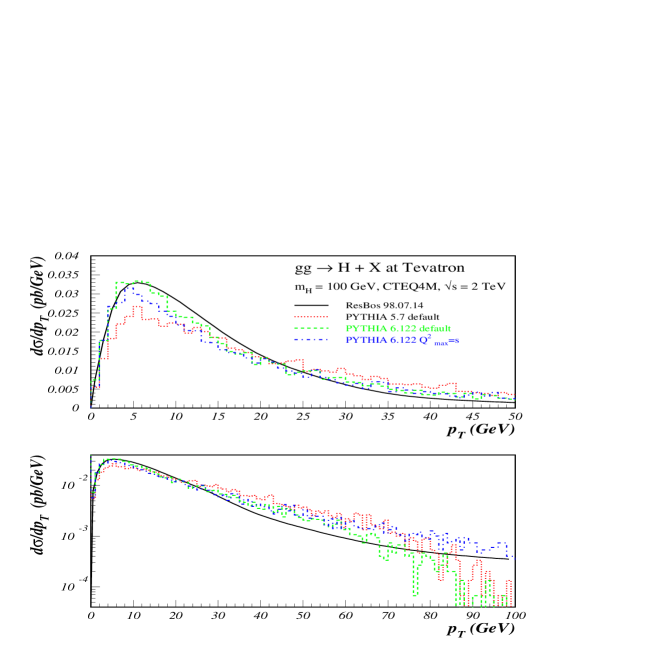
A comparison of the two versions of PYTHIA and of ResBos is also shown in Figure 10 for the case of Higgs production at the Tevatron with center-of-mass energy of 2.0 TeV (for a hypothetical SM Higgs mass of 100 GeV) .  The same qualitative features are observed as at the LHC: the newer version of PYTHIA agrees better with ResBos in describing the low $p_{T}$ shape, and there is a falloff at high $p_{T}$ unless the larger virtuality is used for the parton showers. The default (rms) value of the non-perturbative $k_{T}$ (0.44 GeV) was used for the PYTHIA predictions for Higgs production.

VII Comparison with HERWIG

The variation between versions 5.7 and 6.1 of PYTHIA gives an indication of the uncertainties due to the types of choices that can be made in Monte Carlos. The prescription that $\hat{u}$ be negative for all branchings is a choice rather than an absolute requirement. Perhaps the better agreement of version 6.1 with ResBos is an indication that the adoption of the $\hat{u}$ restrictions was correct. Of course, there may be other changes to PYTHIA which would also lead to better agreement with ResBos for this variable.

FIG. 11.: A comparison of predictions for the Higgs $p_{T}$ distribution at the LHC from ResBos, a recent version of PYTHIA, and HERWIG. All predictions have been normalized to the same area. The bottom figure shows the same in logarithmic scale.

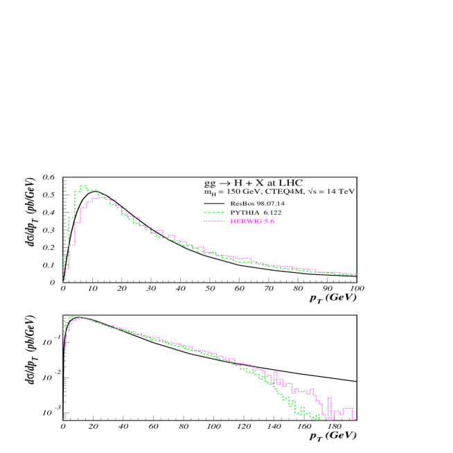
Since there are a variety of choices that can be made in Monte Carlo implementations, it is instructive to compare the predictions for the $p_{T}$ distribution for Higgs production from ResBos and PYTHIA with that from HERWIG version 5.6. The HERWIG prediction, for the Higgs $p_{T}$ distribution at the LHC, is shown in Figure 11, along with the PYTHIA and ResBos predictions, all normalized to the ResBos prediction.  (In all cases, the CTEQ4M parton distribution was used.) The predictions from HERWIG and PYTHIA 6.1 are very similar, with the HERWIG prediction matching the ResBos shape somewhat better at low $p_{T}$. It is interesting that HERWIG matches the ResBos prediction so closely without the implementation of any kinematic cuts as in PYTHIA 6.1. Perhaps the reason is related to the treatment of color coherence in the HERWIG parton showering algorithm. For reference, the absolutely normalized predictions from ResBos, PYTHIA, and HERWIG for the $p_{T}$ distribution of a 150 GeV Higgs at the LHC are shown in Figure 12.

FIG. 12.: A comparison of predictions for the Higgs $p_{T}$ distribution at the LHC from ResBos, two recent versions of PYTHIA, and HERWIG. All predictions have their absolute normalizations. The bottom figure shows the same in logarithmic scale.

VIII Non-perturbative $k_{T}$

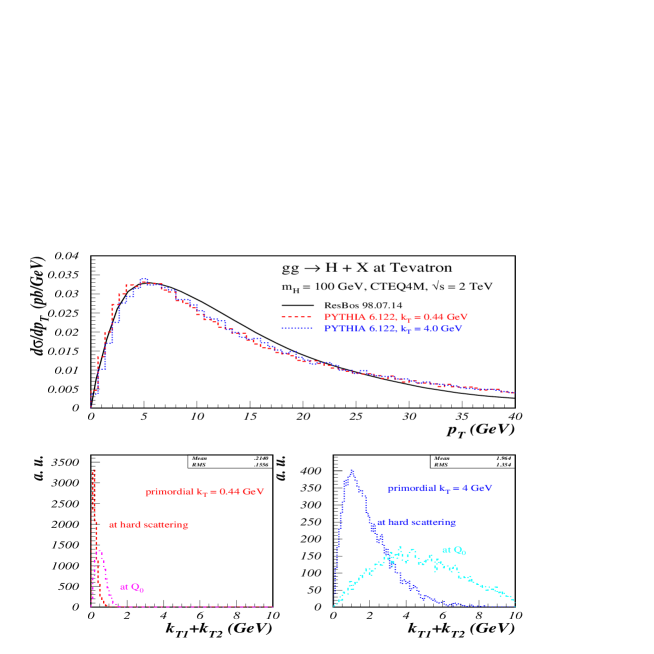
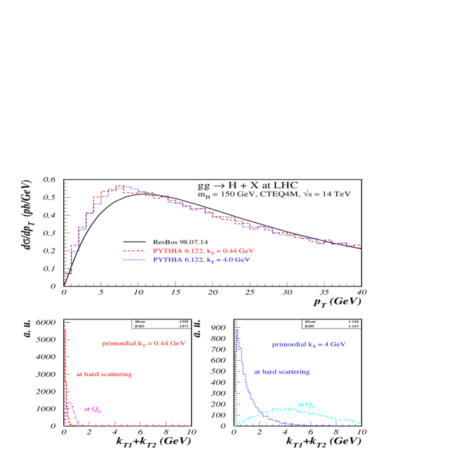
A question still remains as to the appropriate input value of non-perturbative $k_{T}$ in the Monte Carlos to achieve a better agreement in shape, both at the Tevatron and at the LHC.  In Figures 13 and 14 are shown comparisons of ResBos and PYTHIA predictions for the Higgs $p_{T}$ distribution at the Tevatron and the LHC. The PYTHIA prediction (version 6.1 alone) is shown with several values of non-perturbative $k_{T}$. Surprisingly, no difference is observed between the predictions with the different values of $k_{T}$, with the peak in PYTHIA always being somewhat below that of ResBos. This insensitivity can be understood from the plots at the bottom of the two figures, which show the sum of the non-perturbative partonic initial state $k_{T}$’s ($k$_T1+$k$_T2) at $Q_{0}$ and at the hard scatter scale $Q$. Most of the $k_{T}$ is radiated away, with this effect being larger (as expected) at the LHC. The large gluon radiation probability from a $gg$ initial state and the greater phase space available at the LHC lead to a stronger degradation of the non-perturbative $k_{T}$ than was observed with $Z^{0}$ production at the Tevatron.

FIG. 13.: (top) A comparison of the PYTHIA predictions for the $p_{T}$ distribution of a 100 GeV Higgs at the Tevatron using the default (rms) non-perturbative $k_{T}$ (0.44 GeV) and a larger value (4 GeV), at the initial scale $Q_{0}$ and at the hard scatter scale. Also shown is the ResBos prediction. (bottom) The vector sum of the intrinsic $k_{T}$ ($k$_T1+ $k$_T2) for the two initial state partons at the initial scale $Q_{0}$ and at the hard scattering scale, for the two values of primordial $k_{T}$.

FIG. 14.: (top) A comparison of the PYTHIA predictions for the $p_{T}$ distribution of a 150 GeV Higgs at the LHC using the default (rms) non-perturbative $k_{T}$ (0.44 GeV) and a larger value (4 GeV), at the initial scale $Q_{0}$ and at the hard scatter scale. Also shown is the ResBos prediction. (bottom) The vector sum of the intrinsic $k_{T}$ ($k$_T1+$k$_T2) for the two initial state partons at the initial scale $Q_{0}$ and at the hard scattering scale, for the two values of primordial $k_{T}$.

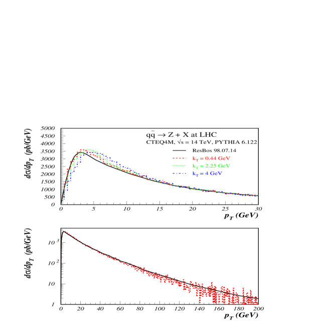
For completeness, a comparison of PYTHIA and ResBos is shown in Figure 15 for $Z^{0}$ boson production at the LHC. There are two points that are somewhat surprising. First, there is still a very strong sensitivity to the value of the non-perturbative $k_{T}$ used in the smearing. Second, the best agreement with ResBos is obtained with the default value (0.44 GeV), in contrast to the 2.15 GeV needed at the Tevatron (cf. Fig1). Note again the agreement of PYTHIA with ResBos at the highest values of $Z^{0}$ $p_{T}$ due to the explicit matrix element corrections applied.

FIG. 15.: A comparison of the predictions for the $p_{T}$ distribution for $Z^{0}$ production at the LHC from PYTHIA and ResBos, where several values of $k_{T}$ have been used to make the PYTHIA predictions.

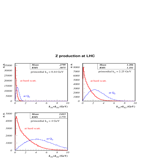
The sum of the incoming parton $k_{T}$ distributions, both at the scale $Q_{0}$ and at the hard scattering scale, are shown in Figure 16 for several different starting (rms) values of primordial $k_{T}$ (per parton). There is substantially less radiation for a $q\overline{q}$ initial state than for a $gg$ initial state (as in the case of the Higgs), leading to a noticeable dependence of the $Z^{0}$ $p_{T}$ distribution on the primordial $k_{T}$ distribution.

FIG. 16.: A comparison of the total initial state $k_{T}$ ($k$_T1+$k$_T2) distributions for $Z^{0}$ production at the LHC from PYTHIA, both at the initial scale $Q_{0}$ and at the hard scattering scale, for several (rms) values of the initial state $k_{T}$. The mean and rms numbers refer to the values at the hard scattering scale.

IX Conclusions

An understanding of the signature for Higgs boson production at either the Tevatron or the LHC depends upon the understanding of the details of the multiple soft–gluon emission from the initial state partons. This soft–gluon radiation can be modeled either in a Monte Carlo or by an analytic resummation calculation, with various choices possible in both implementations. A comparison of the two approaches helps in understanding their strengths and weaknesses, and their reliability. The data from the Tevatron that either exist now, or will exist in Run 2, and from the LHC will be extremely useful to test both methods.

X Acknowledgements

We would like to thank Stefano Catani, Claude Charlot, Gennaro Corcella, Steve Mrenna, and Torbjörn Sjöstrand for useful conversations. We thank Willis Sakumoto for providing the figures for CDF $Z^{0}$ production, and Valeria Tano for HERWIG curves. C.B. and J.H. thank C.-P. Yuan for numerous discussions and blackboard lectures. This work was supported in part by DOE under grant DE-FG-03-94ER40833, and by NSF under grant PHY-9901946.

At the final stage of preparing this manuscript, we became aware of a new preprint [36], which studied the $A$ and $B$ functions for Higgs production up to $O(\alpha_{S}^{4})$, and presented an expression for the coefficient $B^{(2)}$.

REFERENCES

- [1] Proceedings of Physics at Run 2: Workshop on Supersymmetry and Higgs, Summary Meeting, Batavia, IL, Nov. 19-21, 1998.
- [2] S. Abdullin, M. Dubinin, V. Ilyin, D. Kovalenko, V. Savrin and N. Stepanov, Phys. Lett. B431, 410 (1998) [hep-ph/9805341].
- [3] C. Balázs, P. Nadolsky, C. Schmidt and C.–P. Yuan, hep-ph/9905551.
- [4] C. Balázs and C. P. Yuan, Phys. Rev. D59, 114007 (1999) [hep-ph/9810319].
- [5] C. Balázs and C.–P. Yuan, hep-ph/0001103.
- [6] T. Sjöstrand, Phys. Lett. B157, 321 (1985).
- [7] T. Sjöstrand, Comput. Phys. Commun. 82, 74 (1994).
- [8] G. Marchesini, B.R. Webber, G. Abbiendi, I.G. Knowles, M.H. Seymour and L. Stanco, Comput. Phys. Commun. 67, 465 (1992).
- [9] F.E. Paige, S.D. Protopescu, H. Baer and X. Tata, hep-ph/9810440.
- [10] ATLAS Detector and Physics Performance Technical Design Report, CERN/LHCC/99-14.
- [11] J.C. Collins and D.E. Soper, Phys. Rev. Lett. 48, 655 (1982); Nucl. Phys. B193, 381 (1981), B213, 545(E) (1983); B197, 446 (1982); J.C. Collins, D.E. Soper and G. Sterman, Nucl. Phys. B250, 199 (1985). For the application of the low factorization formalism to boson and diphoton production see: [4, 13, 31], and C. Balázs, Ph.D. thesis, Michigan State University (1999), hep-ph/9906422.
- [12] C. Balázs, J.C. Collins and D.E. Soper, “Generalized factorization and resummation”, in the proceedings of the Workshop on Physics at TeV Colliders, Les Houches, France, June 8-18, 1999.
- [13] C. Balázs and C.–P. Yuan, Phys. Rev. D56, 5558 (1997) [hep-ph/9704258].
- [14] F. Landry, R. Brock, G. Ladinsky and C.–P. Yuan, hep-ph/9905391.
- [15] C.–P. Yuan, Phys. Lett. B283, 395 (1992).
- [16] C. Balázs, hep-ph/0008160.
- [17] M. Grazzini, private communication. C. Schmidt, private communication.
- [18] S. Catani and B.R. Webber, Nucl. Phys. B349, 635 (1991).
- [19] G. Miu and T. Sjöstrand, Phys. Lett. B449, 313 (1999).
- [20] G. Corcella and M.H. Seymour, RAL-TR-1999-051 and hep-ph/9908388.
- [21] H. Baer and M. H. Reno, Phys. Rev. D44, 3375 (1991); D45, 1503 (1992).
- [22] S. Mrenna, hep-ph/9902471.
- [23] T. Affolder et al. [CDF Collaboration], Phys. Rev. Lett. 84, 845 (2000) [hep-ex/0001021].
- [24] G. Corcella, talk at the LHC workshop, October 1999.
- [25] H.L. Lai, J. Huston, S. Kuhlmann, F. Olness, J. Owens, D. Soper, W.K. Tung, and H. Weerts, Phys. Rev. D55, 1280 (1997).
- [26] T. Sjöstrand, private communication.
- [27] G. Ladinsky, C.–P. Yuan, Phys. Rev. D50, 4239 (1994).
- [28] F. Abe et al., Phys. Rev. Lett. 70, 2232 (1993); T. Takano, Ph.D. thesis, U. Tsukuba (1998); CDF Collaboration, paper in preparation.
- [29] W. Chen, Ph.D. thesis, State University of New York, Stony Brook, NY (1997); D0 Collaboration, paper in preparation.
- [30] P. Aurenche, A. Douri, R. Baier, and M. Fontannaz, Z. Phys. C29, 423 (1985); B. Bailey, J. Owens, and J. Ohnemus, Phys. Rev. D46, 2018 (1992); T. Binoth, J.P. Guillet, E. Pilon, and M. Werlen, hep-ph/9911340.
- [31] C. Balázs, E.L. Berger, S. Mrenna and C.–P. Yuan, Phys. Rev. D57, 6934 (1998) [hep-ph/9712471];
- [32] PYTHIA manual update for version 6.1, http://www.thep.lu.se/torbjorn/Pythia.html.
- [33] G. Corcella, private communication.
- [34] S. Mrenna, talk at the Physics at Run 2: Workshop on Supersymmetry and Higgs, Summary Meeting, Batavia, IL, Nov. 19-21, 1998; C. Balázs, J. Huston, S. Mrenna, and I. Puljak, in the proceedings of Physics at Run 2: Workshop on Supersymmetry and Higgs, Summary Meeting, Batavia, IL, Nov. 19-21, 1998.
- [35] H. Baer and M. H. Reno, Phys. Rev. D54, 2017 (1996) [hep-ph/9603209].
- [36] D. de Florian and M. Grazzini, hep-ph/0008152.