Limits on a Composite Higgs Boson

Precision electroweak data are generally believed to constrain the Higgs boson mass to lie below approximately 190 GeV at 95% confidence level. The standard Higgs model is, however, trivial and can only be an effective field theory valid below some high energy scale characteristic of the underlying non-trivial physics. Corrections to the custodial isospin violating parameter $T$ arising from interactions at this higher energy scale dramatically enlarge the allowed range of Higgs mass. We perform a fit to precision electroweak data and determine the region in the $(m_{H},\Delta T)$ plane that is consistent with experimental results. Overlaying the estimated size of corrections to $T$ arising from the underlying dynamics, we find that a Higgs mass up to 500 GeV is allowed. We review two composite Higgs models which can realize the possibility of a phenomenologically acceptable heavy Higgs boson. We comment on the potential of improvements in the measurements of $m_{t}$ and $M_{W}$ to improve constraints on composite Higgs models.

Precision electroweak data are generally believed to constrain the Higgs boson mass to lie below approximately 190 GeV at 95% confidence level [1, 2]. The standard Higgs model is, however, trivial [3] and can only be an effective field theory valid below some high energy scale $\Lambda$ characteristic of the underlying non-trivial physics. Additional interactions coming from the underlying theory, and suppressed by the scale $\Lambda$, give rise to model-dependent corrections to measured electroweak quantities. When potential corrections from physics at higher energy scales are included, the limit on the Higgs boson mass becomes weaker [5, 6].

In the context of the triviality of the standard model and given the relatively weak (logarithmic) dependence of electroweak observables on the Higgs boson mass [7], the typical size of corrections to $T$ arising from custodial symmetry violating [8] non-trivial underlying physics can dramatically enlarge the allowed Higgs mass range [6]. In this note we perform a fit to precision electroweak data and determine the region in the $(m_{H},\Delta T)$ plane that is consistent with experimental results. Overlaying the predicted size of corrections to $T$ arising from the underlying dynamics, we find that a Higgs mass up to 500 GeV is allowed. We review two composite Higgs models which can realize the possibility of a phenomenologically acceptable heavy Higgs boson.

For a given Higgs boson mass, an upper bound on the scale $\Lambda$ is given by the position of the Landau pole [10] of the Higgs boson self-coupling $\lambda$. As the Higgs boson mass is proportional to $\lambda(m_{H})$, the larger the Higgs boson mass the smaller the upper bound on the scale $\Lambda$. We may estimate this upper bound by integrating the one-loop beta function for the self-coupling $\lambda$, which yields [10]

$$\Lambda\stackrel{{\scriptstyle<}}{{\sim}}m_{H}\exp\left({4\pi^{2}v^{2}\over 3m^{2}_{H}}\right)~{},$$ (1.1)

where $m_{H}$ is the Higgs boson mass and $v\approx 246$ GeV is the vacuum expectation value of the Higgs boson.

The leading corrections to electroweak observables from the underlying theory are encoded in dimension six operators [12] which contribute to the Peskin-Takeuchi $S$ and $T$ parameters [13]. Given the scale of the underlying non-trivial physics, dimensional analysis [14] may be used to estimate the size of effects from these dynamics in the low-energy Higgs theory [9]. If the underlying theory does not respect custodial symmetry [8], the contribution to $T$ is dominant and is estimated to be

$$|\Delta T|\simeq{b\kappa^{2}\,v^{2}\over\alpha_{em}(M^{2}_{Z})\,\Lambda^{2}},$$ (1.2)

or larger [14]. Here $\alpha_{em}$ is the electromagnetic coupling renormalized at $M^{2}_{Z}$, $b$ is a model-dependent coefficient of order 1, and $\kappa$ is a measure of the size of dimensionless couplings in the effective Higgs theory and is expected to lie between 1 and $4\pi$ [14]. Combining eqn. 1.2 with the bound on $\Lambda$ shown in eqn. 1.1, we find

$$|\Delta T|\stackrel{{\scriptstyle>}}{{\sim}}{b\kappa^{2}\,v^{2}\over\alpha_{em}(M^{2}_{Z})\,m^{2}_{H}}\,\exp\left({-\,{8\pi^{2}v^{2}\over 3m^{2}_{H}}}\right)~{}.$$ (1.3)

Since the Higgs model is trivial, the potential effects of the underlying non-trivial dynamics must be included when establishing constraints on the Higgs mass [6]. As the contributions to $T$ are expected to dominate, we have performed a fit to electroweak measurements [2] and have determined the region in the $(m_{H},\Delta T)$ plane that is consistent with these results. In addition to measurements at the $Z$-pole from LEP and SLD, we include measurements of $M_{W}$ from LEP and the Tevatron, and measurements of $m_{t}$ from the Tevatron. In performing these fits, we have used ZFITTER 6.21 [15] to generate the standard model predictions for a given value of the $Z$ mass, Higgs mass, top-quark mass, and strong ($\alpha_{s}$) and electromagnetic ($\alpha_{em}$) couplings, and have introduced the effect of non-zero $\Delta T$ linearly [16]. We have included the determinations of $\alpha_{em}$ [17]

$$\alpha^{-1}_{em}(M^{2}_{Z})=128.905\pm 0.036$$ (1.4)

and the (non-electroweak) determinations of $\alpha_{s}$ [4]

$$\alpha_{s}(M^{2}_{Z})=0.119\pm 0.002$$ (1.5)

as observations, i.e. we have included deviations from the listed central values in our computation of $\chi^{2}$. The correlation matrices listed in ref. [2] are incorporated in our calculation of $\chi^{2}$.

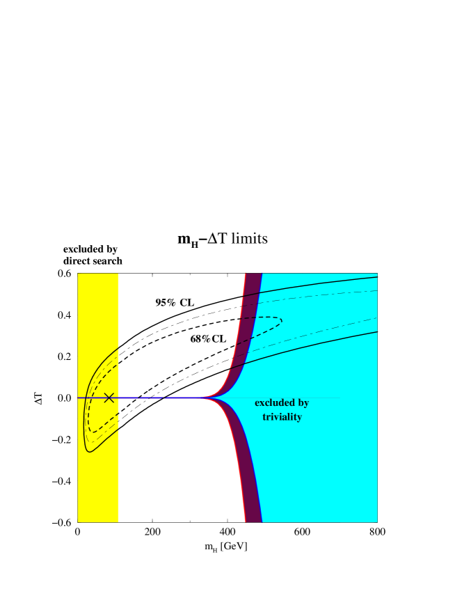
Figure 1: 68% and 95% CL bounds in the $(m_{H},\Delta T)$ plane allowed by a fit to precision electroweak data [1, 2]. The best fit “standard model” value is shown by the cross on the $\Delta T=0$ line. (Also shown by the dot-dash curve is the contour corresponding to $\Delta\chi^{2}=4$, whose intersection with the line $\Delta T=0$ – at approximately 190 GeV – corresponds to the usual 95% CL upper bound quoted on the Higgs boson mass in the standard model.) The light region to the right is excluded by eqn. 1.3 for $b\kappa^{2}=4\pi$. The dark region denotes the additional area excluded for $b\kappa^{2}=4\pi^{2}$. The positive branches of the curves bounding these regions are lower bounds for $\Delta T$ in the top-seesaw and composite higgs models described in the text. Any $(m_{H},\Delta T)$ with positive $\Delta T$ and to the left of the appropriate triviality curve can be realized in the corresponding model.

The result of our fit is summarized in Figure 1. The best-fit value is shown and occurs at a Higgs boson mass of 90 GeV; it corresponds to a minimum value of $\chi^{2}=21.7$ for 21 observables while varying 5 fit parameters ($M_{Z}$, $m_{H}$, $m_{t}$, $\alpha_{s}$, and $\alpha_{em}$). For two degrees of freedom, the 68% and 95% CL bounds correspond to $\Delta\chi^{2}$ of 2.30 and 6.17 respectively. The two degree of freedom 95% CL upper bound on $m_{H}$ is 243 GeV for $\Delta T=0$.

Extending this bound to non-zero $\Delta T$, we see that the region in the $(m_{H},\Delta T)$ plane which fits the observed data as well as the “standard model” at 95% CL extends to large Higgs masses for a positive value of $\Delta T$.

It is not possible, however, for this entire region to be realized consistent with the constraints of triviality. For example, motivated by the models we consider below, the area excluded by eqn. 1.3 with $b\kappa^{2}=4\pi$ is shown as the light region on the right in Figure 1. Overlaying the constraints, we see that Higgs masses above 500 GeV would likely imply the existence of new physics at such low scales ($\Lambda\stackrel{{\scriptstyle<}}{{\sim}}12$ TeV from eqn. 1.1) as to give rise to a contribution to $T$ which is too large [9].

We emphasize that these estimates are based on dimensional arguments, and we are not arguing that it is impossible to construct a composite Higgs model consistent with precision electroweak tests with $m_{H}$ greater than 500 GeV. Rather, barring accidental cancellations in a theory without a custodial symmetry, contributions to $\Delta T$ consistent with eqn. 1.3 are generally to be expected. This expectation is illustrated in the two models which we now discuss.

The top-quark seesaw theory of electroweak symmetry breaking [19, 20] provides a simple example of a model with a potentially heavy composite Higgs boson consistent with electroweak data. In this case, electroweak symmetry breaking is due to the condensation, driven by a strong topcolor [21] gauge interaction, of the left-handed top-quark with a new right-handed singlet fermion $\chi$. Such an interaction gives rise to a composite Higgs field at low energies, and the mass of the top-color gauge boson sets the scale of the Landau pole $\Lambda$ [22]. The weak singlet $\chi_{L}$ and $t_{R}$ fields are introduced so that the $2\times 2$ mass matrix,

$$\left(\begin{array}[]{cc}0&m_{t\chi}\\ m_{\chi t}&m_{\chi\chi}\end{array}\right)$$ (1.6)

is of seesaw form and has a light eigenvalue corresponding to the observed top quark. The value of $m_{t\chi}$ is related to the weak scale, and its value is estimated to be 600 GeV [19].

The coupling of the top-quark to $\chi$ violates custodial symmetry in the same way that the top-quark mass does in the standard model. The leading contribution to $T$ from the underlying top seesaw physics arises from contributions to $W$ and $Z$ vacuum polarization diagrams involving the $\chi$. This contribution is positive and is calculated to be [19, 20]

$$\Delta T={N_{c}\over 16\pi^{2}\alpha_{em}(M^{2}_{Z})}\,{m^{4}_{t\chi}\over m^{2}_{\chi\chi}v^{2}}\approx{0.7\over\alpha_{em}}\left({\Lambda^{2}\over m^{2}_{\chi\chi}}\right)\,\left({v^{2}\over\Lambda^{2}}\right)~{},$$ (1.7)

which is of the form of eqn. 1.2 with $b\kappa^{2}\propto(\Lambda/m_{\chi\chi})^{2}$. Note that $\Lambda/m_{\chi\chi}$ cannot be small since top-color gauge interactions must drive $t\chi$ chiral symmetry breaking. Taking $\Lambda/m_{\chi\chi}\approx 4$, we reproduce the positive branch of the boundary of the light region excluded by triviality shown in Figure 1. By varying $\Lambda$ and $m_{\chi\chi}$, the entire allowed $(m_{H},\Delta T)$ region with positive $\Delta T$ and to the left of the triviality constraint can be obtained. In particular, we note that it is possible to obtain a light Higgs boson in this context as well.

The fact that contributions to $T$ greatly expand the region of allowed Higgs mass in the top seesaw model is discussed in detail in ref. [20]. Here we see that the running of the Higgs self-coupling encoded in the constraints of eqn. 1.3 prevent Higgs masses higher than about 500 GeV from being realized [9].

“Composite Higgs Models” [23] also provide examples of theories with a potentially heavy composite Higgs boson. In the simplest of these models, one introduces three new fermions which couple to a vectorial “ultracolor” $SU(N)$ gauge interaction. Two of these fermions ($\psi$) transform as a vectorial doublet under $SU(2)_{W}$, while the third ($\sigma$) is assumed to be a singlet. Dirac mass terms can be introduced for all of these fermions and, as so far described, chiral symmetry breaking driven by the ultracolor interactions leaves the vectorial $SU(2)_{W}\times U(1)_{Y}$ unbroken. Extra chiral interactions are then introduced to misalign the vacuum by a small amount, causing a nonzero $\bar{\psi}\sigma$ condensate and breaking the weak interactions.

The octet of pions which result from ultracolor chiral symmetry breaking include a set, the analogs of the kaons, which form a composite Higgs boson. Models can be constructed [24] in which the Higgs boson can formally be as heavy as a TeV (i.e. at tree-level), while the other four pions have masses controlled by the ultracolor scale and can be much heavier.

This simplest model does not have a custodial symmetry. A direct calculation of the $W$ and $Z$ masses yields the positive contribution

$$\Delta T={v^{2}\over 4\,\alpha_{em}(M^{2}_{Z})\,f^{2}}~{}.$$ (1.8)

Here $f$ is the pion decay constant for ultracolor chiral symmetry breaking, the analog of $f_{\pi}$ in QCD. The ultracolor chiral symmetry breaking scale, estimated [14] to be ${\cal O}(4\pi f)$, sets the compositeness scale $\Lambda$ of the Higgs boson. Comparing eqns. 1.2 and 1.8, we see that the contribution to $T$ is of the same form with $b\kappa^{2}\approx 4\pi^{2}$, excluding the light and dark shaded regions to the right in Figure 1. From this we see that phenomenologically acceptable composite Higgs models can be constructed with Higgs masses up to approximately 450 GeV. Again, in this case by varying the Dirac masses of the fermions and adjusting the size of the chiral interaction, it is possible to construct models that realize any $(m_{H},\Delta T)$ to the left of the triviality constraint for positive $\Delta T$.

Figure 2: Prospective 68% and 95% CL bounds in $(m_{H},\Delta T)$ plane allowed by fit to precision electroweak data [2] assuming uncertainty in $M_{W}$ is reduced to 30 MeV and uncertainty in $m_{t}$ is reduced 2 GeV, as may be possible during Run II of the Fermilab Tevatron. All curves are as described in Figure 1.

Finally, we briefly consider the prospects for improving these indirect limits over the next few years. The measurements of $M_{W}$ and $m_{t}$ are likely to be greatly improved during Run II of the Fermilab Tevatron. With an integrated luminosity of 10 fb^-1, it may be possible to reduce the uncertainty in the top mass to 2 GeV and in the $W$ mass to 30 MeV [25]. To illustrate the potential of these measurements, in Figure 2 we plot the 68% and 95% CL bounds in the $(m_{H},\Delta T)$ plane which would be allowed if $M_{W}$ and $m_{t}$ assumed their current “best-fit” values while the uncertainties dropped as projected. Note that although the 95% CL region is somewhat smaller than in Fig. 1 (e.g. the two degree of freedom upper bound on the “standard model” Higgs boson mass – $\Delta T=0$ – drops to ${\cal O}$(180 GeV)), there would still be composite Higgs models consistent with electroweak data with a Higgs boson mass up to 500 GeV for positive $\Delta T$.

In a forthcoming publication [26], we will detail the calculation of corrections to precisely measured electroweak quantities in the two composite Higgs models we reviewed above and consider the complementary constraints arising from bounds on $Z\to b\bar{b}$, flavor-changing neutral currents [9], and CP-violation.

Acknowledgments

We thank Gustavo Burdman, Aaron Grant, Marko Popovic, and Elizabeth Simmons for useful discussions. NE is grateful to PPARC for the sponsorship of an Advanced Fellowship. This work was supported in part by the Department of Energy under grant DE-FG02-91ER40676.

References

- [1] A. Straessner, talk presented at Recontres de Moriond, March 17, 2000.
- [2] LEP Electroweak Working Group, http://lepewwg.web.cern.ch/LEPEWWG/stanmod/lepew99.ps.gz.
- [3] K. G. Wilson, Phys. Rev. B4, 3174 (1971) and Phys. Rev. B4, 3184 (1971); K. G. Wilson and J. Kogut, Phys. Rept. 12, 75 (1974).
- [4] C. Caso et al., Eur. Phys. J. C3, 1 (1998), http://www-pdg.lbl.gov/.
- [5] S. Alam et. al., Phys. Rev. D57, 1577 (1998); G. Sanchez-Colon and J. Wudka, Phys. Lett. B432, 383 (1998); L. Hall and C. Kolda, hep-ph/9904236; R. Barbieri and A. Strumia, Phys. Lett. B462, 144 (1999); J. A. Bagger et. al., hep-ph/9908327; C. Kolda and H. Murayama, hep-ph/0003170.
- [6] R. S. Chivukula and N. Evans, Phys. Lett. B464, 244 (1999).
- [7] See, for example, K. Hagiwara et. al., Eur. Phys. J. C2, 95 (1998).
- [8] M. Weinstein, Phys. Rev. D8, 2511 (1973); P. Sikivie et. al., Nucl. Phys. B173, 189 (1980).
- [9] R. S. Chivukula and E. H. Simmons, Phys. Lett. B388, 788 (1996); R. S. Chivukula et. al., Phys. Lett. B401, 74 (1997).
- [10] R. Dashen and H. Neuberger, Phys. Rev. Lett. 50, 1897 (1983).
- [11] J. Kuti, L. Lin, and Y. Shen, Phys. Rev. Lett. 61, 678 (1988).
- [12] T. Appelquist, Based on lectures presented at the 21st Scottish Universities Summer School in Physics, St. Andrews, Scotland, Aug 10-30, 1980; A. C. Longhitano, Phys. Rev. D22, 1166 (1980) and Nucl. Phys. B188, 118 (1981); W. Buchmuller and D. Wyler, Nucl. Phys. B268, 621 (1986); B. Grinstein and M. B. Wise, Phys. Lett. B265, 326 (1991); H. Georgi, Nucl. Phys. B363, 301 (1991).
- [13] M. E. Peskin and T. Takeuchi, Phys. Rev. Lett. 65, 964 (1990) and Phys. Rev. D46, 381 (1992).
- [14] S. Weinberg, Physica 96A, 327 (1979); A. Manohar and H. Georgi, Nucl. Phys. B234, 189 (1984); H. Georgi, Phys. Lett. B298, 187 (1993).
- [15] D. Bardin et al., hep-ph/9908433.
- [16] C. P. Burgess et. al., Phys. Rev. D49, 6115 (1994).
- [17] R. Alemany et. al., Eur. Phys. J. C2, 123 (1998); M. Davier and A. Hocker, Phys. Lett. B419, 419 (1998); J. H. Kuhn and M. Steinhauser, Phys. Lett. B437, 425 (1998); J. Erler, Phys. Rev. D59, 054008 (1999).
- [18] LEP Electroweak Working Group, E. Ferrer, talk presented at Recontres de Moriond, March 14, 2000.
- [19] B. A. Dobrescu and C. T. Hill, Phys. Rev. Lett. 81, 2634 (1998); R. S. Chivukula et. al., Phys. Rev. D59, 075003 (1999).
- [20] H. Collins, A. Grant, and H. Georgi, Phys. Rev. D61, 055002 (2000).
- [21] C. T. Hill, Phys. Lett. B266, 419 (1991).
- [22] W. A. Bardeen, C. T. Hill, and M. Lindner, Phys. Rev. D41, 1647 (1990).
- [23] D. B. Kaplan and H. Georgi, Phys. Lett. 136B, 183 (1984); D. B. Kaplan et. al., Phys. Lett. 136B, 187 (1984); T. Banks, Nucl. Phys. B243, 125 (1984); H. Georgi and D. B. Kaplan, Phys. Lett. B145, 216 (1984); M. J. Dugan et. al., Nucl. Phys. B254, 299 (1985).
- [24] N. Maekawa, Prog. Theor. Phys. 93, 919 (1995) and Phys. Rev. D52, 1684 (1995).
- [25] tev_2000 Study Group, D. Amidei and R. Brock, http://fnalpubs.fnal.gov/archive/1996/pub/Pub-96-082.ps.
- [26] R. S. Chivukula, C. Hölbling, and N. Evans, manuscript in preparation.