The proton and the photon, who is probing whom in electroproduction?

Abstract

The latest results on the structure of the proton and the photon as seen at HERA are reviewed while discussing the question posed in the title of the talk.

1 INTRODUCTION

The HERA collider, where 27.5 GeV electrons collide with 920 GeV protons, is considered a natural extension of Rutherford’s experiment and the process of deep inelastic $ep$ scattering (DIS) is interpreted as a reaction in which a virtual photon, radiated by the incoming electron, probes the structure of the proton. In this talk I would like to discuss this interpretation and ask the question of who is probing whom [1].

The structure of the talk will be the following: it will start with posing the problem, after which our knowledge about the structure of the proton as seen at HERA [2] will be presented followed by a description of our present understanding of the structure of the photon as seen at HERA and at LEP [3, 4]. Next, an answer to the question posed in the title will be suggested and the talk will be concluded by some remarks about the nature of the interaction between the virtual photon and the proton [5].

2 THE QUESTION - WHO IS PROBING WHOM?

2.1 The process of DIS

The process of DIS is usually represented by the diagram shown in figure 1. If the lepton does not change its identity during the scattering process, the reaction is labeled neutral current (NC), as either a virtual photon or a $Z^{0}$ boson can be exchanged. When the identity of the lepton changes in the process, the reaction is called charged current (CC) and a charged $W^{\pm}$ boson is exchanged. During this talk we will discuss only NC processes.

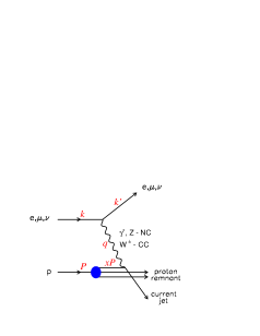
Figure 1: A diagram describing the process of deep inelastic scattering (DIS). The four vector of the incoming and outgoing leptons are $k$ and $k^{\prime}$, that of the exchanged boson is $q$, and that of the incoming proton is $P$. The four momentum of the struck quark is $xP$.

Using the four vectors as indicated in the figure, one can define the usual DIS variables: $Q^{2}=-q^{2}$, the ’virtuality’ of the exchanged boson, $x=Q^{2}/(2P\cdot q)$, the fraction of the proton momentum carried by the interacting parton, $y=(P\cdot q)/(P\cdot k)$, the inelasticity, and $W^{2}=(q+P)^{2}$, the boson-proton center of mass energy squared.

The interpretation of the diagram describing a NC event is the following. The electron beam is a source of photons with virtuality $Q^{2}$. These virtual photons ‘look’ at the proton. Any ‘observed’ structure belongs to the proton. How can we be sure that we are indeed measuring the structure of the proton? Virtual photons have no structure. Is that always true? We know that real photons have structure; we even measure the photon structure function $F_{2}^{\gamma}$ [4]. Let us discuss this point further in the next subsections.

2.2 The fluctuating photon

How is it possible that the photon, which is the gauge particle mediating the electromagnetic interactions, has a hadronic structure? Ioffe’s argument [6]: the photon can fluctuate into $q\bar{q}$ pairs just like it fluctuates into $e^{+}e^{-}$ pairs (see figure 3). If the fluctuation time, defined in the proton rest frame as $t_{f}\simeq(2E_{\gamma})/m^{2}_{q\bar{q}}$, is much larger than the interaction time, $t_{int}\simeq r_{p}$, the photon builds up structure in the interaction. Here, $E_{\gamma}$ is the energy of the fluctuating photon, $m_{q\bar{q}}$ is the mass into which it fluctuates, and $r_{p}$ is the radius of the proton.

Figure 2: Fluctuation of a photon into (a) an $e^{+}e^{-}$ pair, (b) a $q\bar{q}$ pair.

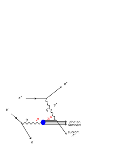
Figure 3: A diagram describing a DIS process on a quasi-real photon using the reaction $e^{+}e^{-}\to e^{+}e^{-}X$.

The hadronic structure of the photon, built during the interaction, can be studied by measuring the photon structure function $F_{2}^{\gamma}$ in a DIS type of experiment where a quasi-real photon is probed by a virtual photon, both of which are emitted in $e^{+}e^{-}$ collisions, as described in figure 3. This diagram is very similar to that in DIS on a proton target (figure 1).

2.3 Structure of virtual photons?

Does a virtual photon also fluctuate and acquire a hadronic structure? The fluctuation time of a photon with virtuality $Q^{2}$ is given by $t_{f}\simeq(2E_{\gamma})/(m^{2}_{q\bar{q}}+Q^{2})$, and thus at very high $Q^{2}$ one does not expect the condition $t_{f}\gg t_{int}$ to hold. However at very large photon energies, or at very low $x$, the fluctuation time is independent of $Q^{2}$: $t_{f}\simeq 1/(2m_{p}x)$, where $m_{p}$ is the proton mass, and thus even highly virtual photons can acquire structure. For instance, at HERA presently $W\sim$ 200 - 300 GeV, and since $x\approx Q^{2}/(Q^{2}+W^{2})$, $x$ can be as low as 0.01 even for $Q^{2}$ = 1000 GeV². In this case, the fluctuation time will be very large compared to the interaction time and the highly virtual photon will acquire a hadronic structure. How do we interprate the DIS diagram of figure 1 in this case? Whose structure do we measure? Do we measure the structure of the proton, from the viewpoint of the proton infinite momentum frame, or do we measure the structure of the virtual photon, from the proton rest frame view? Who is probing whom?

When asked this question, Bjorken answered [7] that physics can not be frame dependent and therefore it doesn’t matter: we can say that we measure the structure of the proton or we can say that we study the structure of the virtual photon. I will try to convince you at the end of my talk that this answer makes sense.

3 THE STRUCTURE OF THE PROTON

In this section we will refrain from discussing the question posed above and will accept the interpretation of measuring the structure of the proton via the DIS diagram in figure 1. We present below information about the structure of the proton as seen from the DIS studies at HERA.

3.1 HERA

With the advent of the HERA $ep$ collider the kinematic plane of $x$-$Q^{2}$ has been extended by 2 orders of magnitude in both variables from the existing fixed target DIS experiments, as depicted in figure 4.

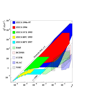
Figure 4: The $x$-$Q^{2}$ kinematic plane of some of the fixed target and of the HERA collider DIS experiments.

The DIS cross section for $ep\to eX$ can be written (for $Q^{2}\ll M_{Z}^{2}$) as [8],

$$\frac{d^{2}\sigma}{dxdQ^{2}}=\frac{4\pi\alpha^{2}}{xQ^{2}}\left\{\frac{y^{2}}{2}2xF_{1}(x,Q^{2})+(1-y)F_{2}(x,Q^{2})\right\}.$$ (1)

In the quark-parton model (QPM), the proton structure function $F_{2}$ is only a function of $x$ and can be expressed as a sum of parton densities, and is related to $F_{1}$ through the Callan-Gross relation [9],

$$F_{2}(x)=\sum_{i}e_{i}^{2}xq_{i}(x)=2xF_{1},$$ (2)

where $e_{i}$ is the electric charge of quark $i$ and the index $i$ runs over all the quark flavours.

Note that in Quantum Chromodynamics (QCD), the Callan-Gross relation is violated, and the structure function is a function of $x$ and $Q^{2}$,

$$F_{2}(x,Q^{2})-2xF_{1}(x,Q^{2})=F_{L}(x,Q^{2})>0,$$ (3)

where the longitudinal structure function $F_{L}$ contributes in an important way only at large $y$.

The motivation for measuring $F_{2}(x,Q^{2})$ can be summarized as follows: (a) test the validity of perturbative QCD (pQCD) calculations, (b) decompose the proton into quarks and gluons, and (c) search for proton substructure.

3.2 QCD evolution - scaling violation

Quarks radiate gluons; gluons split and produce more gluons at low $x$ and also $q\bar{q}$ pairs at low $x$. This QCD evolution chain is usually described in leading order by splitting functions $P_{ij}$, as shown in figure 5.

Figure 5: Splitting functions $P_{ij}$ in leading order, describing the splitting of parton $j$ into parton $i$.

This procedure leads to scaling violation in the following way: there is an increase of $F_{2}$ with $Q^{2}$ at low $x$ and a decrease at high $x$. Scaling holds at about $x$=0.1. The data follows this prediction of QCD, as can be seen in figure 6.

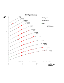
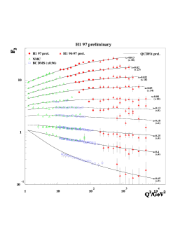
Figure 6: Comparison of the scaling violation behaviour of $F_{2}$ with the results of a next-to-leading order DGLAP evolution equation.

3.3 Overview of $F_{2}$

The fixed target experiments provided information at relatively high $x$ and thus enabled the study of the behaviour of valence quarks. The first HERA results showed a surprisingly strong rise of $F_{2}$ as $x$ decreases. An example of such a rise is given in figure 7 where $F_{2}$ increases as $x$ decreases, for a fixed value of $Q^{2}$ = 15 GeV².

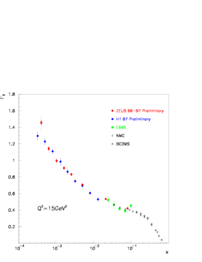
Figure 7: The proton structure function $F_{2}$, as function of $x$, at $Q^{2}$ = 15 GeV², for HERA and some fixed target data.

This increase is the result of the rising gluon density at low $x$. Note the good agreement between both HERA experiments, H1 and ZEUS, and also between HERA and the fixed target data.

3.4 Evolution of $F_{2}$

The measurements of $F_{2}$ as function of $x$ and $Q^{2}$ can be used to obtain information about the parton densities in the proton. This is done by using the pQCD DGLAP evolution equations. One can not calculate everything from first principles but needs as input from the experiment the parton densities at a scale $Q^{2}_{0}$, usually taken as a few GeV², above which pQCD is believed to be applicable.

There are several groups which perform QCD fits, the most notable are MRST [10] and CTEQ [11]. They parameterize the $x$ dependence of the parton densities at $Q^{2}_{0}$ in the form,

$$xq(x,Q^{2})\sim x^{\eta_{1}}\cdot(1-x)^{\eta_{2}}\cdot f_{smooth}(x).$$ (4)

The free parameters like $\eta_{1}$ and $\eta_{2}$ are adjusted to fit the data for $Q^{2}>Q^{2}_{0}$.

Figure 8: $F_{2}$ as function of $x$, for fixed $Q^{2}$ values (in GeV²) as indicated in the figure, for the HERA ’94 data together with some fixed target data. The curves are the result of a NLO QCD fit.

An example of such an evolution study can be seen in figure 8 where the $F_{2}$ data are presented as function of $x$ for fixed $Q^{2}$ values. The increase of $F_{2}$ with decreasing $x$ is seen over the whole range of measured $Q^{2}$ values. The pQCD fits give a good description of the data down to surprisingly low $Q^{2}$ values.

Figure 9: Parton density distributions, as function of $x$, of the MRST global QCD fit, at a scale of $Q^{2}$ = 20 GeV².

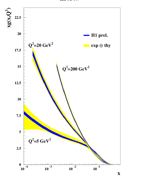
Figure 10: The gluon density distribution, as function of $x$, at $Q^{2}$ = 5, 20 and 200 GeV².

The resulting parton densities from the MRST parameterization at $Q^{2}$ = 20 GeV² are shown in figure 10. One sees the dominance of the $u$ valence quark at high $x$ and the sharp rise of the sea quarks at low $x$. In particular, the gluon density at low $x$ rises very sharply and has a value of more than 20 gluons per unit of rapidity at $x\sim 10^{-4}$. In figure 10 one sees the extracted gluon density by the H1 experiment [12] at three different $Q^{2}$ values. The density of the gluons at a given low $x$ increases strongly with $Q^{2}$.

3.5 Rise of $F_{2}$ with decreasing $x$

The rate of the rise of $F_{2}$ with decreasing $x$ is $Q^{2}$ dependent. This can be clearly seen in figure 12 where $F_{2}$ is plotted as a function of $x$ for three $Q^{2}$ values. The rate of rise decreases as $Q^{2}$ gets smaller.

Figure 11: The proton structure function $F_{2}$, as function of $x$, for three $Q^{2}$ values. The higher the $Q^{2}$, the steeper the distributions.

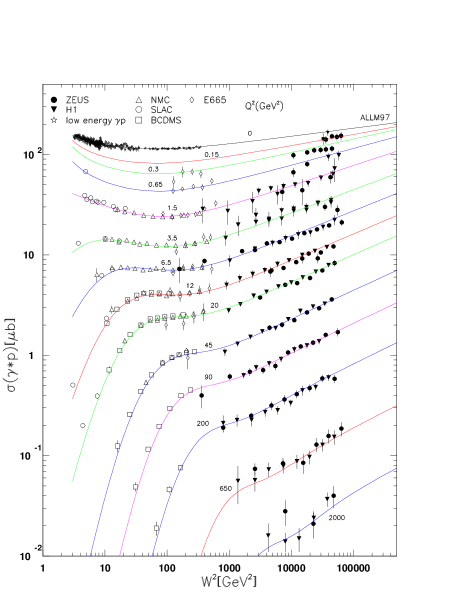
Figure 12: The $\gamma^{*}p$ total cross section $\sigma(\gamma^{*}p)$ as function of $W^{2}$ for fixed values of $Q^{2}$, including the total photoproduction cross section ($Q^{2}$=0). The curves are the results of the ALLM97 parameterization.

What can we say about the rate of rise? To what can one compare it? The proton structure function $F_{2}$ is related to the total $\gamma^{*}p$ cross section $\sigma_{tot}(\gamma^{*}p)$,

$$F_{2}=\frac{Q^{2}(1-x)}{4\pi^{2}\alpha}\frac{Q^{2}}{Q^{2}+4m_{p}^{2}x^{2}}\sigma_{tot}(\gamma^{*}p)\approx\frac{Q^{2}}{4\pi^{2}\alpha}\sigma_{tot}(\gamma^{*}p),$$ (5)

where the approximate sign holds for low $x$. Since we have a better feeling for the behaviour of the total cross section with energy, we plot in figure 12 the $F_{2}$ data converted to $\sigma_{tot}(\gamma^{*}p)$ as function of $W^{2}$ for fixed values of $Q^{2}$. For comparison we plot also the total $\gamma p$ cross section. One sees that the shallow $W$ behaviour of the total $\gamma p$ cross section changes to a steeper behaviour as $Q^{2}$ increases. The curves are the results of the ALLM97 [13] parameterization (see below) which gives a good description of the transition seen in the data.

3.6 The transition region

The data presented above show a clear change of the $W$ dependence with $Q^{2}$. At $Q^{2}$=0 the processes are dominantly non-perturbative and the resulting reactions are usually named as ‘soft’ physics. This domain is well described in the Regge picture. As $Q^{2}$ increases, the exchanged photon is expected to shrink and one expects pQCD to take over. The reactions are said to be ‘hard’. Where does the transition from soft to hard physics take place? Is it a smooth or abrupt one? In the following we describe two parameterizations, one fully based on the Regge picture while the other combines the Regge approach with a QCD motivated one.

3.7 Example of two parameterizations

Donnachie and Landshoff (DL) [14] succeeded to describe all existing hadron-proton total cross section data in a simple Regge picture by using a combination of a Pomeron and a Reggeon exchange, the former rising slowly while the latter decreasing with energy,

$$\sigma_{tot}=Xs^{0.08}+Ys^{-0.45},$$ (6)

where $s$ is the square of the total center of mass energy. The two numerical parameter, related to the intercepts $\alpha(0)$ of the Pomeron and Reggeon trajectories, respectively, are the result of fitting this simple expression to all available data, some of which are shown in the first two plots in figure 13. These parameters give also a good description of the total $\gamma p$ cross section data which were not used in the fit and are also shown on the right hand side of the figure.

Figure 13: The total cross section data of $\bar{p}p,pp,\pi^{\pm}p$ and $\gamma p$ as function of the center of mass energy. The different lines are the results of parameterizations to these data (see text).

Donnachie and Landshoff wanted to extend this picture also to virtual photons [15] (for $Q^{2}<$10 GeV²), keeping the power of $W^{2}$, which is related to the Pomeron intercept, fixed with $Q^{2}$. Their motivation was to see what is the expected contribution from non-perturbative physics, or soft physics as we called it above, at higher $Q^{2}$.

The other example is that of Abramowicz, Levin, Levy, Maor (ALLM) [16], which was updated by Abramowicz and Levy (ALLM97) [13]. This parameterization uses a Regge motivated approach at low $x$ together with a QCD motivated one at high $x$ to parameterize the whole ($x,Q^{2}$) phase space, fitting all existing $F_{2}$ data. This parameterization uses a so-called interplay of soft and hard physics (see [17]) .

Figure 14: The $\gamma^{*}p$ total cross section, as function of $W^{2}$, in bins of $Q^{2}$ for HERA data and that of E665, compared with some parameterizations.

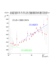
Figure 15: The $Q^{2}$ dependence of the parameter $\lambda$, determined from a fit of the form $F_{2}\sim x^{-\lambda}$ at fixed $Q^{2}$ values.

The two parameterizations are compared [18] to the low $Q^{2}$ HERA data together with that of the fixed target E665 experiment in figure 15. Here one sees again how the cross section changes from a $(W^{2})^{0.08}$ behaviour at very low $Q^{2}$ to a $(W^{2})^{0.2-0.4}$ as $Q^{2}$ increases. The simple DL parameterization as implemented by ZEUS (ZEUSREGGE in the figure) fails to describe the data above $Q^{2}\sim$ 1 GeV². ALLM97 describes the data well in the whole region. DL98 [19], which adds to the soft Pomeron an additional hard Pomeron, can also describe the data, but loses the simplicity of the original DL one.

One can quantify the change in the rate of increase by using the parameter $\lambda$. Since $\sigma_{tot}\sim(W^{2})^{\alpha(0)-1}$ this implies that $F_{2}\sim x^{-\lambda}$. The fitted value of $\lambda$ as function of $Q^{2}$ is shown in figure 15 for the ZEUS [20] (upper) and the H1 [21] (lower) experiments. One sees a clear increase of $\lambda$ with $Q^{2}$ which cannot be reproduced by the simple Regge picture but needs an approach in which there is the interplay of soft and hard physics [17].

3.8 What have we learned about the structure of the proton?

Let us summarize what we have learned so far about the structure of the proton.

• The density of partons in the proton increases with decreasing $x$.

• The rate of increase is $Q^{2}$ dependent; at high $Q^{2}$ the increase follows the expectations from the pQCD hard physics while at low $Q^{2}$ the rate is described by the soft physics behaviour expected by the Regge phenomenology.

• Though there seems to be a transition in the region of $Q^{2}\sim$ 1-2 GeV², there is an interplay between the soft and hard physics in both regions.

4 THE STRUCTURE OF THE PHOTON

In this part we will describe what is presently known about the structure of the photon, both from $e^{+}e^{-}$ experiments as well as from HERA.

4.1 Photon structure from $e^{+}e^{-}$

The hadronic structure function of the photon, $F_{2}^{\gamma}$, was measured in $e^{+}e^{-}$ collisions which can be interpreted as depicted in figure 3. A highly virtual $\gamma^{*}$ with large $Q^{2}$ probes a quasi-real $\gamma$ with $P^{2}\approx$ 0.

The measurements of $F_{2}^{\gamma}$ showed a different behaviour than that of the proton structure function. From the $Q^{2}$ dependence, shown in figure 17 [4], one sees positive scaling violation for all $x$.

Figure 16: The photon structure function $F_{2}^{\gamma}$, as function of $Q^{2}$, for average $x$ values as given in the figure. The curves are the expectations of different parameterizations of parton distributions in the photon.

Figure 17: $F_{2}^{\gamma}$, as function of $x$, for fixed $Q^{2}$ as given in the figure. The data points have been taken from the numerical tables in [4].

This different behaviour can be understood as coming from an additional splitting to the ones present in the proton case (see figure 5). In the photon case, the photon can split into a $q\bar{q}$ pair, $\gamma\to q\bar{q}$. The contribution resulting from this splitting, called the ‘box diagram’, causes positive scaling violation for all $x$. In addition, and again contrary to the proton case, it also causes the photon structure function to be large for high $x$ values, as can be seen in figure 17 where $F_{2}^{\gamma}$ is plotted as function of $x$ for fixed $Q^{2}$ values. From this figure one can also see that there exist very little data in the low $x$ region.

4.2 Photon structure from HERA

At HERA, the structure of the photon can be studied by selecting events in which the exchanged photon is quasi-real and the probe is provided by a large transverse momentum parton from the proton. The probed photon can participate in the process in two ways. In one, the interaction takes place before it fluctuates into a $q\bar{q}$ pair and thus the whole of the photon participates in the interaction. Such a process is called a ‘direct’ photon interaction. In the other case, the photon first fluctuates into partons and only one of these partons participates in the interaction while the rest continue as the photon remnant. This process is said to be a ‘resolved’ photon interaction. An example of leading order diagrams describing dijet photoproduction for the two processes is shown in figure 19.

Figure 18: Examples of leading order QCD (a) ‘direct’ and (b) ‘resolved’ dijet production diagrams.

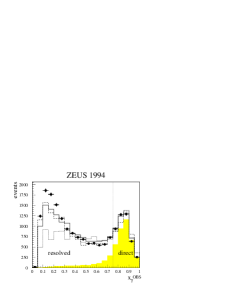
Figure 19: The $x_{\gamma}^{obs}$ distribution, as obtained from photoproduction of dijet events. The shaded area are the expectations of the distribution of this variable from the generation of direct photon events. The dotted vertical line is the border of an operational definition of direct and resolved photon events.

If one defines a variable $x_{\gamma}$ as the fraction of the photon momentum taking part in a dijet process, we expect $x_{\gamma}\sim$ 1 in the direct case, while $x_{\gamma}\ll$ 1 in the resolved photon interaction. These two processes are clearly seen in figure 19 where the $x_{\gamma}$ distribution shows a two peak structure, one coming from the direct photon and the other from the resolved photon interactions [22].

One way of obtaining information about $F_{2}^{\gamma}$ from HERA is to measure the dijet photoproduction as function of $x_{\gamma}$ and to subtract the contribution coming from the direct photon reactions. This is shown in figure 21,

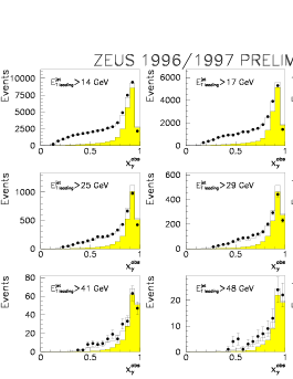
Figure 20: Distributions of $x_{\gamma}^{obs}$, for different thresholds on the highest transverse energy jet. The open histogram is the prediction of the MC, and the shaded part is the direct photon component of the MC.

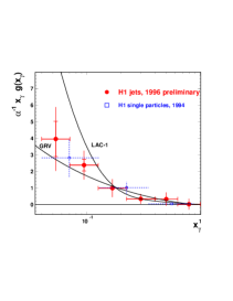
Figure 21: Comparison of the photon gluon density, determined from di-jet photoproduction events taken in 1996, with earlier measurements of H1. The curves are the expectations of different parameterizations.

where the measurements are presented at fixed values of the hard scale, which is taken as the highest transverse energy jet [23]. One can go one step further by assuming leading order QCD and Monte Carlo (MC) models to extract the effective parton densities in the photon. An example of the extracted gluon density in the photon [24] is shown in figure 21. The gluon density increases with decreasing $x$, a similar behaviour to that of the gluon density in the proton. The data have the potential of differentiating between different parameterization of the parton densities in the photon, as can be seen in the same figure.

4.3 Virtual photons at HERA

One can study the structure of virtual photons in a similar way as described above. In this case, the $Q^{2}$ of the virtual photon has to be much smaller than the transverse energy squared of the jet, $E_{t}^{2}$, which provides the hard scale of the probe. Such a study [25] is presented in figure 23, where the dijet cross section is plotted as function of $x_{\gamma}$ for different regions in $Q^{2}$ and $E_{t}^{2}$. One sees a clear excess over the expectation of direct photon reactions, indicating that virtual photons also have a resolved part.

Figure 22: The differential dijet cross section, as function of $x_{\gamma}^{jets}$, for different scales as indicated in the figure. The open histogram is the prediction of the MC and the shaded part is the direct photon component of the MC.

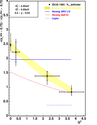
Figure 23: The ratio of the resolved to direct photon component, as function of the virtuality $Q^{2}$ (in GeV²) of the photon.

This fact can also been seen in figure 23 where the ratio of resolved to direct photon interactions is plotted as function of the virtuality $Q^{2}$ of the probed photon [26]. One sees that although the ratio decreases with $Q^{2}$, it remains non-zero even at relatively high $Q^{2}$ values.

4.4 Virtual photons at LEP

The study of the structure of virtual photons in $e^{+}e^{-}$ reactions was dormant for more than 15 years following the measurement done by the PLUTO collaboration [27]. Recently, however, the L3 collaboration at LEP [28] measured the structure function of photons with a virtuality of 3.7 GeV², using as probes photons with a virtuality of 120 GeV².

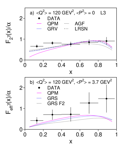
Figure 24: The effective photon structure function from L3 for (a) a quasi-real photon target and (b) a 3.7 GeV² photon target. Both photons were probed at a scale of 120 GeV².

Figure 25: The dependence of the effective photon structure function on the mass $P^{2}$ of the probed photon.

In the same experiment, the structure function of real photons was also measured. Both results can be seen in figure 25 and within errors the structure function of the virtual photons is of the same order of magnitude as that of the real ones. The effective structure function is also presented as function of the virtuality of the probed photon $P^{2}$ in figure 25 and show very little dependence on $P^{2}$ up to values of $\sim$ 6 GeV² [27, 28].

4.5 What have we learned about the structure of the photon?

Let us summarize what we have learned so far about the structure of the photon.

• At HERA one can see clear signals of the 2-component structure of quasi-real photons, a direct and a resolved part.

• Virtual photons can also have a resolved part at low $x$ and fluctuate into $q\bar{q}$ pairs.

• Structure of virtual photons has been seen also at LEP.

5 THE ANSWER

Following the two sections on the structure of the proton and the photon, let us remind ourselves again what our original question was. At low $x$ we have seen that a $\gamma^{*}$ can have structure. Does it still probe the proton in an $ep$ DIS experiment or does one of the partons of the proton probe the structure of the $\gamma^{*}$?

The answer is just as Bjorken said: at low $x$ it does not matter. Both interpretation are correct. The emphasis is however ‘at low $x$’. At low $x$ the structure functions of the proton and of the photon can be related through Gribov factorization [29]. By measuring one, the other can be obtained from it through a simple relation. This can be seen as follows.

Gribov showed [29] that the $\gamma\gamma$, $\gamma p$ and $pp$ total cross sections can be related by Regge factorization as follows:

$$\sigma_{\gamma\gamma}(W^{2})=\frac{\sigma_{\gamma p}^{2}(W^{2})}{\sigma_{pp}(W^{2})}.$$ (7)

This relation can be extended [1] to the case where one photon is real and the other is virtual,

$$\sigma_{\gamma^{*}\gamma}(W^{2},Q^{2})=\frac{\sigma_{\gamma^{*}p}(W^{2},Q^{2})\sigma_{\gamma p}(W^{2})}{\sigma_{pp}(W^{2})},$$ (8)

or to the case where both photons are virtual,

$$\sigma_{\gamma^{*}\gamma^{*}}(W^{2},Q^{2},P^{2})=\frac{\sigma_{\gamma^{*}p}(W^{2},Q^{2})\sigma_{\gamma^{*}p}(W^{2},P^{2})}{\sigma_{pp}(W^{2})}.$$ (9)

Since at low $x$ one has $\sigma\approx\frac{4\pi^{2}\alpha}{Q^{2}}F_{2}$, one gets the following relations between the proton structure function $F_{2}^{p}$, the structure function of a real photon, $F_{2}^{\gamma}$, and that of a virtual photon, $F_{2}^{\gamma^{*}}$:

$$F_{2}^{\gamma}(W^{2},Q^{2})=F_{2}^{p}(W^{2},Q^{2})\frac{\sigma_{\gamma p}(W^{2})}{\sigma_{pp}(W^{2})},$$ (10)

and

$$F_{2}^{\gamma^{*}}(W^{2},Q^{2},P^{2})=\frac{4\pi^{2}\alpha}{P^{2}}\frac{F_{2}^{p}(W^{2},Q^{2})F_{2}^{p}(W^{2},P^{2})}{\sigma_{pp}(W^{2})}.$$ (11)

The relation given in equation (10) has been used [30] to ‘produce’ $F_{2}^{\gamma}$ ‘data’ from well measured $F_{2}^{p}$ data in the region of $x<$0.01, where the Gribov factorization is expected to hold. The results are plotted in figure 26 together with direct measurements of $F_{2}^{\gamma}$. Since no direct measurements exist in the very low $x$ region for $Q^{2}>4$ GeV², it is difficult to test the relation. However both data sets have been used for a global QCD leading order and higher order fits [31] to obtain parton distributions in the photon. Clearly there is a need of more precise direct $F_{2}^{\gamma}$ data for such a study.

Figure 26: The photon structure function, as function of $x$, for fixed $Q^{2}$ values as indicated in the figure. The full points are direct measurements, and the open triangles are those obtained from $F_{2}^{p}$ through the Gribov factorization relation. The full line is the result of a higher order fit and the dashed line is that of a leading order parameterization.

In any case, our answer to the question would be that at low $x$ the virtual photon and the proton probe the structure of each other. In fact, what one probes is the structure of the interaction. At high $x$, the virtual photon can be assumed to be structureless and it studies the structure of the proton.

6 DISCUSSION - THE STRUCTURE OF THE INTERACTION

We concluded in the last section that at low $x$ one studies the structure of the interaction. Let us discuss this point more clearly.

We saw that in case of the proton at low $x$, the density of the partons increases with decreasing $x$. Where are the partons located? In the proton rest frame, Bjorken $x$ is directly related to the space coordinate of the parton. The distance $l$ in the direction of the exchanged photon is given by [6],

$$l=\frac{1}{2m_{p}x}\approx\frac{0.1{\rm fm}}{x}.$$ (12)

Therefore partons with $x>$0.1 are in the interior of the proton, while all partons with $x<$0.1 have no direct relation to the structure of the proton. The low $x$ partons describe the properties of the $\gamma^{*}p$ interaction.

How can we describe a $\gamma^{*}p$ interaction at low $x$? It occurs in two steps: first the virtual photon fluctuates into a $q\bar{q}$ pair and then the configuration of this pair determines if the interaction is ‘soft’ or ‘hard’ [32]. The soft process is the result of a large spatial configuration in which the photon fluctuates into an asymmetric small $k_{T}$ $q\bar{q}$ pair. The hard nature of the interaction is obtain when the fluctuation is into a small configuration of a symmetric $q\bar{q}$ pair with large $k_{T}$. The two configurations are shown in figure 28.

Figure 27: Fluctuation of the photon into a $q\bar{q}$ pair in (a) an asymmetric small $k_{T}$ configuration, (b) a symmetric large $k_{T}$ configuration.

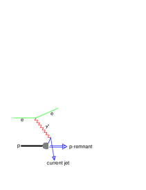
Figure 28: A DIS diagram, as seen from the point of view of a photon fluctuating into an asymmetric pair, in which the fast quark becomes the current jet.

At $Q^{2}$=0 the asymmetric configuration is dominant and the large color forces produce a hadronic component which interacts with the proton and leads to hadronic non-perturbative soft physics. The symmetric component contributes very little; the high $k_{T}$ configuration is screened by color transparency (CT). At higher $Q^{2}$ the contribution of the symmetric small configuration gets bigger. Each one still contributes little because of CT, but the phase space for such configurations increases. Nevertheless, the asymmetric large configuration is also still contributing and thus both soft and hard components are present. Another way to see this interplay is by looking at the diagram in figure 28. In a simple QPM picture of DIS, the fast quark from the asymmetric configuration becomes the current jet while the slow quark interacts with the proton in a soft process. Thus the DIS process looks in the $\gamma^{*}p$ frame just like the $Q^{2}$=0 case. This brings the interplay of soft and hard processes.

7 CONCLUSION

• In DIS experiments at low $x$ one studies the ‘structure’ of the $\gamma^{*}p$ interaction.

• In order to study the interior structure of the proton, one needs to measure the high $x$ high $Q^{2}$ region. This will be done at HERA after the high luminosity upgrade.

I would like to thank Professors K. Maruyama and H. Okuno for organizing a pleasant and lively Symposium. Special thanks are due to Professor K. Tokushuku and his group for being wonderful hosts during my visit in Japan. Finally I would like to thank Professor H. Abramowicz for helpful discussions.

References

- [1] A. Levy, Phys. Lett. B404 (1997) 369.
- [2] For a recent review see H. Abramowicz and A. Caldwell, Rev. Mod. Phys. 71 (1999) 1275.
- [3] J. Butterworth, Structure of the photon to appear in the proceedings of Lepton-Photon 99, [hep-ex/9912030].
- [4] R. Nisius and references therein, The photon structure from deep inelastic electron-photon scattering, [hep-ex/9912049].
- [5] A. Levy, The structure of the Troika: proton, photon and Pomeron, as seen at HERA, Proceedings of the XXIth Workshop on the Fundamental Problems of High Energy Physics and Field Theory, (Eds. V. Petrov and I. Filimonova), p. 7, Protvino 1998, [hep-ph/9811462].
- [6] B.L. Ioffe, Phys. Lett. B30 (1969) 123; B.L.Ioffe, V.A. Khoze and L.N. Lipatov, Hard Processes, (North-Holland, 1984).
- [7] J.D. Bjorken, in response to the question asked at DIS94, Eilat, February 1994.
- [8] See e.g. E. Leader and E. Predazzi, An Introduction to Gauge Theories and the New Physics, (Cambridge University Press, 1982).
- [9] C.G. Callan and D.J. Gross, Phys. Rev. Lett. 22 (1969) 156.
- [10] A.D. Martin, R.G. Roberts, W.J. Stirling and R.S. Thorne, Europ. Phys. J. C4 (1998) 463.
- [11] CTEQ Collab., H.L. Lai et al., Phys. Rev. D55 (1997) 1280.
- [12] M. Klein, Structure Functions in Deep Inelastic Lepton-Nucleon Scattering, to appear in the proceedings of Lepton-Photon 99, [hep-ex/0001059].
- [13] H. Abramowicz and A. Levy, The ALLM parameterization of : an update, DESY 97-251, [hep-ph/9712415].
- [14] A. Donnachie and P.V. Landshoff, Phys. Lett. B296 (1992) 227.
- [15] A. Donnachie and P.V. Landshoff, Zeit. Phys. C61 (1994) 139.
- [16] H. Abramowicz, E. Levin, A. Levy and U. Maor, Phys. Lett. B269 (1991) 465.
- [17] H. Abramowicz, L. Frankfurt and M. Strikman, Surveys in High Energy Phys. 11 (1997) 51.
- [18] C. Amelung for the ZEUS Collab., proceedings of DIS99, Nucl. Phys. B(Proc.Suppl.)79 (1999) 176.
- [19] A. Donnachie and P.V. Landshoff, Phys. Lett. B437 (1998) 408.
- [20] ZEUS Collab., J. Breitweg et al., Europ. Phys. J. C7 (1999) 609.
- [21] J. Zacek for the H1 Collab., proceeding of DIS99, Nucl. Phys. B(Proc.Suppl.)79 (1999) 86.
- [22] ZEUS Collab., M. Derrick et al., Europ. Phys. J. C1 (1998) 109.
- [23] ZEUS Collab., paper 540 submitted to HEP99, Tampere, July 1999.
- [24] J. Cvach for the H1 Collab., proceeding of DIS99, Nucl. Phys. B(Proc.Suppl.)79 (1999) 501.
- [25] H1 Collab., C. Adloff et al., DESY 98-205, to be published in Europ. Phys. J. C, [hep-ex/9812024].
- [26] D. Kcira for the ZEUS Collab., proceedings of Photon99, Freiburg, May 1999.
- [27] PLUTO Collab., Ch. Berger et al., Phys. Lett. B142 (1984) 119.
- [28] F.C Erne for the L3 Collab., proceedings of Photon99, Freiburg, May 1999.
- [29] V.N. Gribov, L.Ya. Pomeranchuk, Phys. Rev. Lett. 8 (1962) 343.
- [30] H. Abramowicz, E. Gurvich and A. Levy, Phys. Lett. B420 (1998) 104.
- [31] H. Abramowicz, E. Gurvich and A. Levy, Next to leading order parton distributions in the photon from and scattering, proceedings of ICHEP98, p.885, Vancouver, July 1998.
- [32] J.D. Bjorken, Final state hadrons in deep inelastic processes and colliding beams, proceedings of the International Symposium on Electron and Photon Interactions at High Energies, p. 281, Cornell, 1971.