Loop-after-loop contribution to the second-order Lamb shift in hydrogenlike low-$Z$ atoms

Abstract

We present a numerical evaluation of the loop-after-loop contribution to the second-order self-energy for the ground state of hydrogenlike atoms with low nuclear charge numbers $Z$. The calculation is carried out in the Fried-Yennie gauge and without an expansion in $Z\alpha$. Our calculation confirms the results of Mallampalli and Sapirstein and disagrees with the calculation by Goidenko and coworkers. A discrepancy between different calculations is investigated. An accurate fitting of the numerical results provides a detailed comparison with analytic calculations based on an expansion in the parameter $Z\alpha$. We confirm the analytic results of order $\alpha^{2}(Z\alpha)^{5}$ but disagree with Karshenboim’s calculation of the $\alpha^{2}(Z\alpha)^{6}\ln^{3}(Z\alpha)^{-2}$ contribution.

Introduction

In the low-$Z$ region, calculations of radiative corrections in bound-state QED have historically relied on a (semi-) analytic expansion in powers of the external binding field $Z\alpha$. Calculations based on this perturbative approach have made an enormous advance during the last 50 years and achieved an excellent agreement with experiments (see, for example, a recent review [1]). However, calculations in higher orders in $Z\alpha$ become increasingly complex, as the number of terms in each higher order increases rapidly. Beside this, it is difficult to estimate the contribution of unevaluated higher-order terms. These are the reasons why the exact numerical treatment of radiative corrections is highly appreciated even in the low-$Z$ region. It allows to test the reliability of methods based on an expansion in $Z\alpha$ and can provide even more accurate results than analytic perturbative calculations. Some examples of this are the calculation of the self-energy correction to the hyperfine splitting in muonium performed by Blundell and coworkers [2], the calculation of the relativistic recoil correction for hydrogen by Shabaev et al. [3], and the evaluation of the first-order self-energy correction for $Z=1-5$ by Jentschura et al. [4].

The aim of the present work is a numerical evaluation of the loop-after-loop contribution to the second-order Lamb shift of the ground state in hydrogen-like atoms to all orders in $Z\alpha$ in the low-$Z$ region. Analytic calculations of the $Z\alpha$-expansion coefficients for this contribution were previously performed by Eides and coworkers [5] and Pachucki [6] in order $\alpha^{2}(Z\alpha)^{5}$ and by Karshenboim [7] in order $\alpha^{2}(Z\alpha)^{6}\ln^{3}(Z\alpha)^{-2}$. The first calculation of the loop-after-loop correction without an expansion in $Z\alpha$ was carried out by Mitrushenkov et al. [8] for high-$Z$ atoms. Recently, this correction was calculated to all orders in $Z\alpha$ for the entire range of nuclear charge numbers by Mallampalli and Sapirstein [9]. A fit to the data from Ref. [9] confirms the analytic result of order $\alpha^{2}(Z\alpha)^{5}$ but it is in a significant disagreement with Karshenboim’s result of order $\alpha^{2}(Z\alpha)^{6}\ln^{3}(Z\alpha)^{-2}$. The subsequent calculation by Goidenko et al. [10], also non-perturbative in $Z\alpha$, shows to be compatible with the analytic calculations. In this work, we perform an independent calculation of the loop-after-loop correction and investigate possible reasons for the discrepancy between different calculations. Relativistic units are used in this article ($\hbar=c=m=1$).

I Basic formalism and numerical procedure

The expression for the irreducible contribution of Fig 1a (we refer to it as the loop-after-loop correction) reads

$$\Delta E_{\rm lal}=\sum_{\varepsilon_{n}\neq\varepsilon_{a}}\frac{\langle a|\Sigma_{R}(\varepsilon_{a})|n\rangle\langle n|\Sigma_{R}(\varepsilon_{a})|a\rangle}{\varepsilon_{a}-\varepsilon_{n}}\ ,$$ (1)

where $\Sigma_{R}$ denotes the renormalized self-energy operator, $|a\rangle$ indicates the initial state and the summation is performed over the spectrum of the Dirac equation. The term with $\varepsilon_{n}=\varepsilon_{a}$ corresponds to the reducible contribution and should be calculated together with the remaining diagrams in Fig. 1. The self-energy operator is defined by its matrix elements

$$\langle a|\Sigma_{R}(\varepsilon)|b\rangle = i\alpha\int^{\infty}_{-\infty}d\omega\int d^{3}{\bf x}_{1}d^{3}{\bf x}_{2}\psi^{{\dagger}}_{a}({\bf x}_{1})$$ (4)

$$\times\alpha_{\mu}G(\varepsilon-\omega,{\bf x}_{1},{\bf x}_{2})\alpha_{\nu}\psi_{b}({\bf x}_{2})D^{\mu\nu}(\omega,{\bf x}_{12})$$

$$-\delta m\int d^{3}{\bf x}\psi^{{\dagger}}_{a}({\bf x})\beta\psi_{b}({\bf x})\ ,$$

where $\alpha_{\mu}=(1,{\mbox{\boldmath$\alpha$}})$; $\beta$, $\alpha$ are the Dirac matrices, $G(\omega)=1/(\omega-{\cal H}(1-i0))$ is the Dirac-Coulomb Green function, ${\cal H}=({\mbox{\boldmath$\alpha$}}\cdot{\bf p})+\beta m+V({\bf x})$ is the Dirac-Coulomb Hamiltonian, $\delta m$ is the mass counterterm, and $D^{\mu\nu}(\omega,{\bf x}_{12})$ is the photon propagator in a general covariant gauge

$$D^{\mu\nu}(\omega,{\bf x}_{12})=\int\frac{d{\bf k}}{(2\pi)^{3}}e^{i{\bf k}{\bf x}_{12}}\left(-\frac{g^{\mu\nu}}{{\rm k}^{2}+i0}+\left.(1-\lambda)\frac{{\rm k}^{\mu}{\rm k}^{\nu}}{({\rm k}^{2}+i0)^{2}}\right)\right|_{{\rm k}^{0}=\omega}\ .$$ (5)

To our knowledge, up to now all the practical self-energy calculations without an expansion in $Z\alpha$ were carried out in the Feynman gauge ($\lambda=1$) which is technically the easiest choice of the gauge. While the usage of the Feynman gauge in calculations of the self-energy matrix elements is natural in the high-$Z$ region, for low $Z$ it is known to provide a spurious contribution of order $Z\alpha$ which should be cancelled numerically to give a residual of order $(Z\alpha)^{4}$. This spurious term is known to vanish in the Fried-Yennie gauge [11, 12] ($\lambda=3$), which possesses remarkable infrared properties. Since the present work is aimed to a calculation of the loop-after-loop correction in the low-$Z$ region, we use the fact that this contribution is invariant in any covariant gauge and perform our calculations in the Fried-Yennie gauge.

A general method which was used here for the calculation of the self-energy matrix elements can be found in Ref. [13], with some modifications due to a non-diagonal nature of the matrix elements and the different gauge. The self-energy matrix element is considered as a sum of two contributions originating from an expansion of the bound electron propagator in terms of interactions with the external field of the nucleus

$$\langle a|\Sigma_{R}(\varepsilon)|b\rangle=\langle a|\Sigma^{(0+1)}_{R}(\varepsilon)|b\rangle+\langle a|\Sigma^{(2+)}(\varepsilon)|b\rangle\ .$$ (6)

Here, the first term contains zero and one Coulomb interaction with the nucleus, and the second term contains two and more interactions. They are calculated in momentum and coordinate space, respectively.

The expression (1) for the loop-after-loop contribution contains a summation of non-diagonal self-energy matrix elements over the whole spectrum of the Dirac equation. To perform the summation, we use the B-splines method for the Dirac equation developed by Johnson et al. [14]. In this method, the infinite summation in the spectral representation of the Green function with a fixed angular momentum quantum number is replaced by a finite sum over basis-set functions. A straightforward evaluation of the sum in Eq. (1) implies a computation of many self-energy matrix elements with highly-oscillating wave functions and is computationally intensive. To reduce the computational time significantly, we define a self-energy correction to the wave function, as proposed in Ref. [8]

$$|\varphi_{SE}\rangle\equiv\Sigma_{R}(\varepsilon_{a})|a\rangle\ .$$ (7)

According to Eqs. (6) and (7), we write Eq. (1) as

$$\Delta E_{\rm lal} = \int\frac{d^{3}{\bf p}_{1}}{(2\pi)^{3}}\frac{d^{3}{\bf p}_{2}}{(2\pi)^{3}}{\varphi_{SE}^{(0+1)}}^{{\dagger}}({\bf p}_{1})G^{\rm red}(\varepsilon_{a},{\bf p}_{1},{\bf p}_{2})\varphi_{SE}^{(0+1)}({\bf p}_{2})$$ (10)

$$+2\int\frac{d^{3}{\bf p}_{1}}{(2\pi)^{3}}d^{3}{\bf x}_{2}{\varphi_{SE}^{(0+1)}}^{{\dagger}}({\bf p}_{1})G^{\rm red}(\varepsilon_{a},{\bf p}_{1},{\bf x}_{2})\varphi_{SE}^{(2+)}({\bf x}_{2})$$

$$+\int d^{3}{\bf x}_{1}d^{3}{\bf x}_{2}{\varphi_{SE}^{(2+)}}^{{\dagger}}({\bf x}_{1})G^{\rm red}(\varepsilon_{a},{\bf x}_{1},{\bf x}_{2})\varphi_{SE}^{(2+)}({\bf x}_{2})\ ,$$

where $G^{\rm red}(\varepsilon_{a},{\bf x}_{1},{\bf x}_{2})$, $G^{\rm red}(\varepsilon_{a},{\bf p}_{1},{\bf p}_{2})$, and $G^{\rm red}(\varepsilon_{a},{\bf p}_{1},{\bf x}_{2})$ are the reducible Dirac-Coulomb Green functions in coordinate, momentum, and mixed representations, respectively (by the mixed representation we mean the Fourier transform over one coordinate variable).

As the first step of the numerical evaluation of Eq. (10), the effective wave functions $\varphi_{SE}^{(0+1)}({\bf p})$ and $\varphi_{SE}^{(2+)}({\bf x})$ are calculated on a grid and stored in an external file. Their computation is not much more intensive than an evaluation of a single self-energy matrix element. The most difficult part of the calculation is the evaluation of $\varphi_{SE}^{(2+)}({\bf x})$. Working in the Fried-Yennie gauge, we do not encounter severe cancellations between zero-, one-, and many-potential terms, as occur in the case of the Feynman gauge. Still, significant cancellations arise in the computation of the Green function $G^{(2+)}$ which contains two and more interactions with the external field. In our implementation it is evaluated by a point-by-point subtraction of the two first terms of the Taylor expansion from the Dirac-Coulomb Green function (see Ref. [13] for details)

$$G^{(2+)}(\varepsilon,x_{1},x_{2})=G(\varepsilon,x_{1},x_{2})-\left.G(\varepsilon,x_{1},x_{2})\right|_{Z=0}-Z\left(\left.\frac{d}{dZ}G(\varepsilon,x_{1},x_{2})\right|_{Z=0}\right)\ .$$ (11)

To control the cancellations which arise in the low-$Z$ region, we monitor the corresponding Wronskian difference $\Delta_{\kappa}^{(2+)}(\varepsilon)$ which can be calculated analytically ($\Delta_{\kappa}(\varepsilon)$ is the Wronskian of the solutions of the radial Dirac equation). Another numerical problem is the partial wave expansion. Its convergence is somewhat slower in the case of the Fried-Yennie gauge than in the Feynman gauge. In actual calculations we extended the summation up to sixty partial waves. It was performed before all numerical integrations were carried out. The remainder after the truncation of the sum was estimated taking into account the asymptotic behaviour of the expansion terms. Several checks were made of calculations of $\varphi_{SE}^{(0+1)}({\bf p})$ and $\varphi_{SE}^{(2+)}({\bf x})$. In one, we compared the diagonal self-energy matrix elements to the known results for the first-order self-energy contribution [15, 4]. We also calculated the irreducible contribution to the self-energy correction to the hyperfine splitting in H-like atoms and found a good agreement with Ref. [2].

In the next step, we perform the radial integrations in Eq. (10). The Dirac-Coulomb Green function in coordinate space is evaluated using a finite basis set constructed from B-splines, after a transformation to a piecewise-polynomial representation as described in the Appendix. The momentum and the mixed representations of the Green function are obtained by the direct numerical Fourier transformation of the polynomial basis. After that, two-dimensional radial integrals in Eq. (10) are expressed as a linear combination of one-dimensional integrals and can be easily evaluated up to a desirable precision. In actual calculations we used a basis set consisting of 70 positive and 70 negative energy states. The stability of the final results with respect to the size of the cavity and the number of energy states was checked.

II Numerical results and discussion

In Table I and Fig. 2 we present the results of our calculation of the loop-after-loop contribution to the second-order Lamb shift of the ground state of hydrogenlike atoms, expressed in the standard form

$$\Delta E_{\rm lal}=\left(\frac{\alpha}{\pi}\right)^{2}\frac{(Z\alpha)^{5}}{n^{3}}G_{\rm lal}(Z\alpha)\ .$$ (12)

The results of two previous non-perturbative calculations of this correction are presented in Table I and Fig. 2 as well. A comparison exhibits a good agreement of the present calculation with the results of Mallampalli and Sapirstein [9] and a strong deviation from the results of Goidenko et al. [10].

Let us consider possible reasons for this discrepancy. The method used in Ref. [10] is based on the multiple commutator approach combined with the partial-wave renormalization (PWR) procedure. In the PWR method, the truncation of the partial-wave expansion fulfils the role of the regularization parameter. This shows that this method is non-covariant. Still, it can be used for the calculation of the diagonal first-order self-energy matrix elements, for which the PWR procedure is known to provide the correct result [16, 17]. In Ref. [18] this renormalization procedure was investigated for the self-energy correction to an additional Coulomb screening potential. It was shown analytically that some spurious terms arise in different parts of the total self-energy correction due to the non-covariant nature of the renormalization procedure. According to Ref. [18], the spurious terms cancel each other if the perturbation is the Coulomb potential. The cancellation of the spurious contributions in the total self-energy correction holds no longer if the perturbation contains a magnetic photon (see Ref. [19] and a conclusion remark in Ref. [18]).

To consider this topic in more detail, we calculate the self-energy correction in the presence of the perturbing potential $-\alpha/r$ both in the PWR scheme and using a covariant renormalization. For this choice of a perturbing potential, the total self-energy correction for a state $|a\rangle$ is $d/(dZ)\langle a|\Sigma_{R}(\varepsilon_{a})|a\rangle$. The results of calculations are listed in Table II. Our calculation confirms the conclusions from Ref. [18] about $a)$ the presence of spurious terms in different parts of the correction and $b)$ their cancellation in the sum for this particular choice of a perturbing potential. Summarizing, we conclude that it is possible that the PWR method applied to the irreducible part of the second-order self-energy correction, can provide a nonzero spurious contribution.

In order to compare our results with calculations based on an expansion in $Z\alpha$, we approximate our data for the function $G_{\rm lal}$ by a least-squares fit with five parameters $a_{50}$, $a_{63}$, $a_{62}$, $a_{61}$, and $a_{60}$ (the first index of the $a$ coefficients indicates the power of $Z\alpha$, the second corresponds to the power of $\ln(Z\alpha)^{-2}$). A fit to our numerical results in Table I yields

$$a_{50}=2.33\mbox{\hskip 28.45274pt}a_{63}=-1.1\ .$$ (13)

This is in a good agreement with the fitting coefficients from Ref. [9] ($a_{50}=2.3$ or $2.8$ for different sets of data, $a_{63}=-0.9$) but disagrees significantly with Karshenboim’s analytic result $a_{63}=-8/27$ [7].

In order to investigate this discrepancy in more detail, we note that the $Z\alpha$-expansion calculations of the loop-after-loop correction in Refs. [5, 6, 7] were performed in the Fried-Yennie gauge like in the present work and, therefore, it is possible to compare the calculations on intermediate stages. So, we expand the inner electron propagators in diagram Fig. 1a in terms of interactions with the nuclear binding potential and calculate the first six terms of the expansion separately. The corresponding Feynman diagrams are presented in Fig. 3. These diagrams do not contain $\varphi_{SE}^{(2+)}({\bf x})$ which is the most difficult part of the calculation. Therefore, we were able to calculate them for very low fractional $Z$. This is important for a reliable fitting of our data which vary very fast in the vicinity of $Z=0$. The remainder behaves more smoothly in the low-$Z$ region and its fitting is easier. In the calculation of the diagrams shown in Fig. 3, we use closed analytical expressions for the Dirac Green function with zero and one Coulomb interaction. In this way we eliminate the numerical uncertainty due to the finite basis set representation of the Green function. The numerical results for each diagram in Fig. 3 were approximated by least-squares fits with eight or seven parameters $a_{50}$, $a_{6i}$ ($i=3,\ldots,0$), $a_{7i}$ ($i=3,2,1$) (in the last case $a_{71}$ was omitted). In order to reduce the statistical uncertainty of the fitting procedure, a large number of points (twenty or more) was used. The stability of the fitting coefficients was checked with respect to the number of points, minimal and maximal nuclear charge numbers, and different fits. The numerical results and the fitting coefficients for diagrams in Fig. 3 are listed in Table III.

We found a good agreement with results from Refs. [5, 6] for the coefficient $a_{50}$ and with Ref. [7] for the coefficient $a_{63}$ originating from diagram Fig. 3f. The only discrepancy with the analytical calculations originates from diagram Fig. 3c. While this diagram should not contribute to order $\alpha^{2}(Z\alpha)^{6}\ln^{3}(Z\alpha)^{-2}$ according to Karshenboim, our calculation shows the presence of a cubed logarithm with coefficient $a_{63}=-0.652(30)$.

Summarizing, we conclude that our calculation of the loop-after-loop correction confirms the analytic result of Refs. [5, 6] for the coefficient $a_{50}$ ($a_{50}=2.3$). A fit to the numerical results yields

$$a_{63}=-0.958(30)\mbox{\hskip 28.45274pt}a_{62}=3.3(5)$$ (14)

for the diagrams shown in Fig. 3, and

$$a_{63}=-0.05(7)\mbox{\hskip 28.45274pt}a_{62}=1.2(8)$$ (15)

for the non-perturbative remainder.

We note a remarkably slow convergence of the $Z\alpha$-expansion for the loop-after-loop contribution to the second-order Lamb shift. As an illustration, in Fig. 4 we plot the contributions of the first one, two, and three expansion terms together with the non-perturbative results. The expansion coefficients are taken from Eqs. (14) and (15). One can see that even for hydrogen the contribution of the first three expansion terms covers only about 50% of the total result. To obtain a reasonable fit to the numerical data even for very low $Z$, it is necessary to take into account at least four first expansion terms. This fact shows the necessity for non-perturbative (in $Z\alpha$) calculations of the total second-order Lamb shift in the low-$Z$ region.

Piecewise-polynomial representation of the Green function

The B-splines method for the Dirac equation [14] provides a finite set of radial wave functions with a fixed angular momentum quantum number which can be written in the form

$$\varphi_{\kappa,n}^{i}(x)=\frac{1}{x}\sum_{k}c^{i}_{k}(\kappa,n,l)\,(x-x_{l})^{k}\ ,$$ (16)

assuming that $x\in\left[x_{l},x_{l+1}\right]$. Here $x_{l}$ is the radial grid, the index $i=1,2$ indicates the upper and the lower component of the radial wave function, $n$ numbers the wave functions in the set, and $\kappa$ is the angular momentum quantum number. The radial Green function, defined by

$$G^{ij}_{\kappa}(\varepsilon,x_{1},x_{2})=\sum_{n}\frac{\varphi_{\kappa,n}^{i}(x_{1})\varphi_{\kappa,n}^{j}(x_{2})}{\varepsilon-\varepsilon_{n}}\ ,$$ (17)

can be written in the piecewise-polynomial representation as follows:

$$G_{\kappa}^{ij}(\varepsilon,x_{1},x_{2})=\frac{1}{x_{1}x_{2}}\sum_{k_{1}k_{2}}A^{ij}_{k_{1}k_{2}}(\varepsilon,\kappa,l_{1},l_{2})(x-x_{l_{1}})^{k_{1}}(x-x_{l_{2}})^{k_{2}}\ ,$$ (18)

where $x_{1}\in\left[x_{l_{1}},x_{l_{1}+1}\right]$, $x_{2}\in\left[x_{l_{2}},x_{l_{2}+1}\right]$. The coefficients $A^{ij}_{k_{1}k_{2}}$ are

$$A^{ij}_{k_{1}k_{2}}(\varepsilon,\kappa,l_{1},l_{2})=\sum_{n}\frac{c^{i}_{k_{1}}(\kappa,n,l_{1})c^{j}_{k_{2}}(\kappa,n,l_{2})}{\varepsilon-\varepsilon_{n}}\ .$$ (19)

The radial Green function in momentum space can be written in the same way using Fourier transformed basic polynomials

$$G^{ij}_{\kappa}(\varepsilon,p_{1},p_{2}) = \sum_{l_{1}l_{2}}\sum_{k_{1}k_{2}}A^{ij}_{k_{1}k_{2}}(\varepsilon,\kappa,l_{1},l_{2})\Pi^{ik_{1}}_{l_{1}}(p_{1})\Pi^{jk_{2}}_{l_{2}}(p_{2})\ ,$$ (20)

$$\Pi^{ik}_{l}(p) = 4\pi s(L_{i})\int_{x_{l}}^{x_{l+1}}dx\,x(x-x_{l})^{k}j_{L_{i}}(px)\ ,$$ (21)

where $L_{1,2}=|\kappa\pm 1/2|-1/2$; $s(L_{1})=1$, $s(L_{2})=-\kappa/|\kappa|$; and $j_{L}(z)$ denotes the spherical Bessel function.

FIG. 1.: One-electron self-energy Feynman diagrams of second order in $\alpha$.

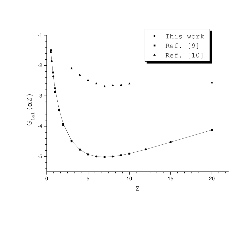
FIG. 2.: The function $G_{\rm lal}(Z\alpha)$ in different calculations. The solid line indicates a fit to our numerical results.

FIG. 3.: Diagrams obtained from Fig. 1a by expansion of the inner electron propagators in terms of interactions with the nuclear binding potential. A double line denotes the electron in the field of the nucleus. A single line indicates the free electron. A dashed line denotes a Coulomb interaction with the nucleus. Some diagrams are counted twice, as is denoted by ”(2)”.

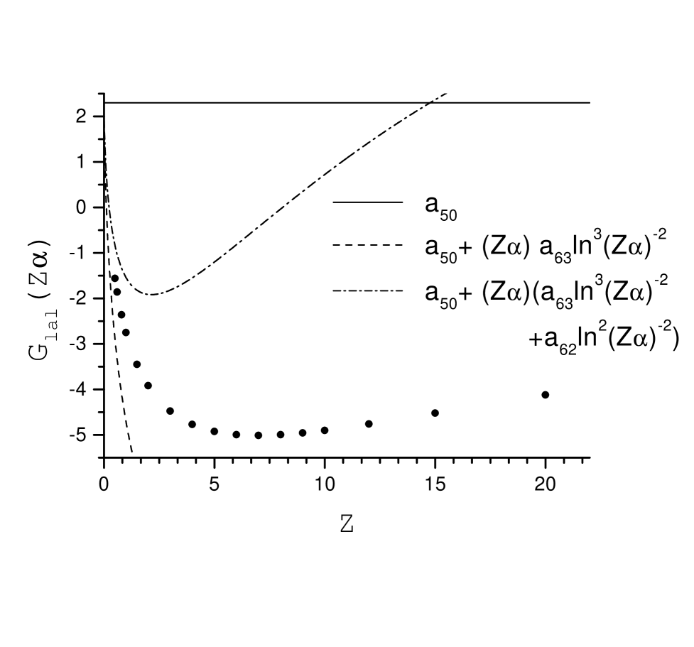
FIG. 4.: The non-perturbative (in $Z\alpha$) function $G_{\rm lal}(Z\alpha)$ and the contributions of the first one, two, and three terms of its expansion in $Z\alpha$. Dots indicate the non-perturbative results. The expansion coefficients are taken from Eqs. (14) and (15).

REFERENCES

- [1] K. Pachucki, Hyp. Int. 114, 55 (1998).
- [2] S. A. Blundell, K. T. Cheng, J. Sapirstein, Phys. Rev. Lett. 78, 4914 (1997).
- [3] V. M. Shabaev, A. N. Artemyev, T. Beier, G. Soff, J. Phys. B 31, L337 (1998).
- [4] U. D. Jentschura, P. J. Mohr, G. Soff, Phys. Rev. Lett. 82, 53 (1999).
- [5] M. I. Eides, S. G. Karshenboim, V. A. Shelyuto, Phys. Lett. B 312, 358 (1993); Physics of Atomic Nuclei 57, 1240 (1994).
- [6] K. Pachucki, Phys. Rev. Lett. 72, 3154 (1994).
- [7] S. G. Karshenboim, Zh. Eksp. Teor. Fiz. 103, 1105 (1993) [Sov. Phys. JETP 76, 541 (1993)].
- [8] A. Mitrushenkov, L. Labzowsky, I. Lindgren, H. Persson, S. Salomonson, Phys. Lett. A 200, 51 (1995).
- [9] S. Mallampalli and J. Sapirstein, Phys. Rev. Lett. 80, 5297 (1998).
- [10] I. Goidenko, L. Labzowsky, A. Nefiodov, G. Plunien, G. Soff, Phys. Rev. Lett 83, 2312 (1999).
- [11] A. A. Abrikosov, Zh. Eksp. Teor. Fiz. 30, 96 (1956) [Sov. Phys. JETP 3, 71 (1956)].
- [12] H. M. Fried, D. R. Yennie, Phys. Rev. 112, 1391 (1958).
- [13] V. A. Yerokhin, V. M. Shabaev, Phys. Rev. A 60, 800 (1999).
- [14] W. R. Johnson, S. A. Blundell, J. Sapirstein, Phys. Rev. A 37, 307 (1988).
- [15] P. J. Mohr, Phys. Rev. A 46, 4421 (1992).
- [16] H. Persson, I. Lindgren, and S. Salomonson, Phys. Scr. T 46, 125 (1993).
- [17] H. M. Quiney and I. P. Grant, Phys. Scr. T 46, 132 (1993); J. Phys. B 27, L299 (1994).
- [18] H. Persson, S. Salomonson, and P. Sunnergren, Adv. Quant. Chem. 30, 379 (1998).
- [19] V. A. Yerokhin, A. N. Artemyev, and V. M. Shabaev, Phys. Lett. A 234, 361 (1997).