Oblique Parameter Constraints on Large Extra Dimensions

Abstract

We consider the Kaluza-Klein scenario in which gravity propagates in the $4+n$ dimensional bulk of spacetime and the Standard Model particles are confined to a 3-brane. We calculate the gauge boson self-energy corrections arising from the exchange of virtual gravitons and present our results in the $STU$-formalism. We find that the new physics contributions to $S$, $T$ and $U$ decouple in the limit that the string scale $M_{S}$ goes to infinity. The oblique parameters constrain the lower limit on $M_{S}$. Taking the quantum gravity cutoff to be $M_{S}$, $S$-parameter constraints impose $M_{S}>1.55$ TeV for $n=2$ at the 1$\sigma$ level. $T$-parameter constraints impose $M_{S}>1.25\ (0.75)$ TeV for $n=3\ (6)$.

I Introduction

The possible existence of extra dimensions has been a fascinating idea in physics ever since Kaluza-Klein theory was proposed [1]. Consistent string theories demand the existence of extra dimensions [2]. However, if the string scale ($M_{S}$) is as high as the grand unification scale ($M_{\rm GUT}\sim 10^{16}$ GeV) or the Planck scale ($M_{\rm Pl}\sim 10^{19}$ GeV), as is the case for a weakly coupled heterotic string, then the length scale of the compactified extra dimensions $(R\sim 1/M_{S})$ would be too small to be appreciable experimentally. Recent developments in string theory indicate that the string scale can be much lower than the Planck scale and even close to the electroweak scale [3]. This possibility provides new avenues towards many theoretical issues such as alternative solutions to the gauge hierarchy problem [4, 5], fermion mass and flavor mixings [6], and new inflationary cosmological models [7]. More importantly, such a scenario may lead to a rich phenomenology and is thus experimentally testable at low energies [8, 9, 10, 11, 12].

Assume that there are $n$ extra dimensions in which only gravity can propagate while Standard Model (SM) fields are confined to four dimensional spacetime. The large value of the Planck scale can be understood by Gauss’ law from the relation

$$M_{\rm Pl}^{2}\sim R^{n}M_{S}^{n+2}\ ,$$ (1)

where the string scale $M_{S}$ is taken to be the Planck mass in $4+n$ dimensions. For $M_{S}\sim{\cal O}$ (1 TeV), $R$ can range from 1 fm to 1 mm for $n=6$ to 2 [4]. There are no direct gravitational tests sensitive to those small scales yet [13]. Such large extra dimensions manifest themselves only through interactions involving the Kaluza-Klein (KK) modes of the gravitons with enhanced coupling strength after summing over the many contributing light KK states. The effective theory governing the graviton couplings to matter was described in [9, 10]. Phenomenological studies showed that future collider experiments can provide constraints on $M_{S}$ typically of order 1 TeV, depending on the collider center of mass energies [9, 11, 12]. Astrophysical (cosmological) considerations have been used to impose lower bounds on $M_{S}$ to be about 30 (100) TeV for $n=2$ and very weak bounds for higher dimensions [14].

In this paper we consider radiative corrections to the masses of the electroweak gauge bosons $(W,Z)$ arising from the exchange of massive spin-2 KK gravitons. The motivation for this study is two-fold. Firstly, a rigorously renormalizable theory of gravity does not exist. It would be interesting to explore to what extent the formalism in Ref. [9, 10] is finite against radiative corrections in the sense of an effective field theory. An early attempt in Ref. [10] for a scalar self-energy correction showed that the radiative corrections are proportional to the scalar mass, instead of the ultraviolet cutoff. Another one-loop calculation for the muon $g-2$ also reached finite results [15]. Secondly, if one is able to compute radiative effects from KK gravitons, one may hope to examine constraints on new physics characterized by the string scale from precision electroweak measurements. In fact, a recent paper appeared to estimate the $\rho$ parameter [16], which was found to be both ultraviolet and infrared divergent. However, our results arrive at completely different conclusions.

The rest of the paper is organized as follows. In Section II we compute one-loop self-energy diagrams for a gauge boson from exchange of massive spin-2 KK gravitons. To do so, we need to derive the four–point couplings of two gravitons and two gauge bosons which are beyond that given in Ref. [9, 10] and have been left out in the previous calculations [15, 16]. In Section III we adopt the $STU$-formalism [17] and constrain the string scale based on current experimental values of the oblique parameters. Computing oblique parameters has an advantage over calculating $W(Z)$ mass corrections directly since they are free of certain technical and conceptual uncertainties. We discuss our results and conclude in Section IV. In two appendices we present the relevant Feynman rules and describe the regularization of the infrared divergences.

II Self-energy corrections to the gauge bosons

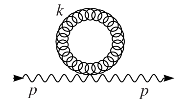
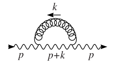
FIG. 1.: The seagull and rainbow diagrams contributing to the self-energy of gauge bosons.

When the typical energy scale of interest is much smaller than the string scale $M_{S}$, the compactified higher dimensional theory can be described by an effective theory where only relevant light degrees of freedom are retained, namely, those related to the so called Kaluza-Klein states. In principle, if only gravity is of higher dimensional origin, spin-0, 1 and 2 KK states can arise [9, 10]. The spin-1 states decouple from the Standard Model fields and make no contribution to the self-energies. Naively, one expects the spin-0 contributions to be of the same order of magnitude as that of the spin-2 states since they have the same coupling strength. However, the properties of the spin-0 states are model-dependent since there is no symmetry to protect their masses. In the following we shall concentrate on the spin-2 KK states (which we will call KK gravitons).

The physical process that we consider in this paper is the radiative corrections to the weak gauge boson masses at the one-loop level from these KK gravitons. We focus our attention on the transverse part of the self-energy $\Pi_{XY}(p^{2})$ between gauge bosons $X$ and $Y$, as it is the only part relevant to us. These self-energies are written as

$$\Pi_{Z}(p^{2})\equiv\Pi^{T}_{ZZ}(p^{2})\quad{\rm and}\quad\Pi_{W}(p^{2})\equiv\Pi^{T}_{WW}(p^{2}).$$ (2)

Note that both $\Pi_{Z\gamma}$ and $\Pi_{\gamma\gamma}$ are identically zero, following from the simple fact that they must be proportional to the photon mass, as required by the gravitational nature of the KK graviton-matter interactions.

There are two diagrams contributing to the self-energy of a gauge boson, as shown in Fig. 1. The first (seagull diagram) involves a four–point coupling of two KK gravitons and two gauge bosons, and the second (rainbow diagram) involves two three–point couplings of a KK graviton and two gauge bosons. These two diagrams are at the same order in the gravitational coupling $\kappa^{2}=16\pi G_{N}$, where $G_{N}$ is the usual four-dimensional Newton’s constant.

To obtain the four-point vertex Feynman rule required for the seagull diagram, one needs to expand the graviton-matter interaction Lagrangian to order $\kappa^{2}$, which is beyond the order of the expansion given in [10]. We provide this Feynman rule in Appendix A. The corresponding seagull diagram is purely transverse, proportional to $(\eta_{\mu\nu}-p_{\mu}p_{\nu}/p^{2})\ \Pi_{S}(p^{2})$, with

$$\Pi_{S}(p^{2})\ =\ {\frac{\kappa^{2}p^{2}}{16\pi^{2}}}\sum_{\vec{n}}\int_{0}^{\infty}{\frac{dk_{E}^{2}\,k_{E}^{2}}{k_{E}^{2}+m_{\vec{n}}^{2}}}\left({\frac{k_{E}^{4}}{12m_{\vec{n}}^{4}}}+{\frac{3k_{E}^{2}}{4m_{\vec{n}}^{2}}}+{3\over 2}\right)\ ,$$ (3)

where we have included a factor $1/2$ to avoid double-counting when we sum over the KK modes and the subscript $E$ indicates that the variable is in Euclidean space. The summation over the KK modes in a tower can be written as an integration because of the near-degeneracy of the KK states,

$$\sum_{\vec{n}}f(m_{\vec{n}})=\int_{0}^{\infty}dm_{\vec{n}}^{2}\rho(m_{\vec{n}})f(m_{\vec{n}})$$ (4)

where

$$\rho(m_{\vec{n}})={\frac{R^{n}m_{\vec{n}}^{n-2}}{(4\pi)^{n/2}\,\Gamma(n/2)}}$$ (5)

is the KK state density. By convention for the torus compactification [10], the relation between the four-dimensional Newton’s constant and the $(4+n)$-dimensional string scale $M_{S}$ is given by

$$\kappa^{2}R^{n}=8\pi(4\pi)^{n/2}\,\Gamma(n/2)M_{S}^{-(n+2)}.$$ (6)

Using Eqs. (4), (5) and  (6), we obtain

$${\frac{\kappa^{2}}{16\pi^{2}}}\sum_{\vec{n}}f(m_{\vec{n}})={\frac{1}{2\pi M_{S}^{n+2}}}\int_{0}^{\infty}dm_{\vec{n}}^{2}\,m_{\vec{n}}^{n-2}f(m_{\vec{n}}^{2}).$$ (7)

The above sum is divergent in the ultraviolet for $n\geq 2$ unless $f(m_{\vec{n}})$ falls off very rapidly with $m_{\vec{n}}^{2}$. Since the effective theory is only expected to be valid below the string scale, we introduce an explicit cutoff $\lambda M_{S}$ to regularize the mass sum, where $\lambda\sim{\cal O}(1)$ and parameterizes the sensitivity to the cutoff. We shall use the same cutoff for the momentum integral as for the mass summation. We believe that this regulator will best reflect the ultraviolet behavior of the divergence. Our final result for the seagull diagram is

$$\Pi_{S}(p^{2})={\frac{\lambda^{n+2}p^{2}}{12\pi}}\int_{0}^{1}\int_{0}^{1}dxdy~{}{\frac{x\,{y^{-3+{\frac{n}{2}}}}}{x+y}}\,\left(x+3\,y\right)\,\left(x+6\,y\right)\ ,$$ (8)

where $x=(k_{E}/\lambda M_{S})^{2}$ and $y=(m_{\vec{n}}/\lambda M_{S})^{2}$.

The necessary Feynman rules for calculating the rainbow diagram have been derived in [10] and are summarized in Appendix A. The complete expression for the general $\Pi_{R}(p^{2})$ is lengthy and unilluminating. We will instead present the special cases relevant to our current consideration, $\Pi_{R}(0)$ and $\Pi_{R}(m^{2})$. The former can be written as

$$\Pi_{R}(0) = {\frac{\lambda^{n+2}m^{2}}{24\pi}}\int_{0}^{1}\int_{0}^{1}dxdy~{}{\frac{x\,{y^{-3+{\frac{n}{2}}}}}{\left(r+x\right)\left(x+y\right)}}\times$$ (10)

$$\biggl{[}x\left(x+y\right)\left(x+13y\right)+r\left(4{x^{2}}+26xy+52{y^{2}}\right)\biggr{]}\ ,$$

where we have introduced a dimensionless mass ratio between the gauge boson mass and the ultraviolet cutoff $r=(m/\lambda M_{S})^{2}$. Similarly,

$$\Pi_{R}(m^{2}) = {\frac{\lambda^{n+2}m^{2}}{24\pi}}\int_{0}^{1}\int_{0}^{1}\int_{0}^{1}dxdydz~{}\,{\frac{x\,{y^{-3+{\frac{n}{2}}}}\ F(x,y,z,r)}{{{[x+y(1-z)+r\,{z^{2}}]}^{2}}}}\ ,$$ (11)

where $z$ is a Feynman parameter and

$$F(x,y,z,r) = 4\,{r^{3}}\,{{\left(-2+z\right)}^{2}}\,{z^{4}}+{r^{2}}\,{z^{2}}\,\biggl{[}16y(-2+z)+x(-24+52z-21{z^{2}})\biggr{]}$$ (14)

$$+r\biggl{[}4xy(2-8z+{z^{2}})+4{y^{2}}(4+9{z^{2}})+{x^{2}}(1-14\,z+15{z^{2}})\biggr{]}$$

$$-x({x^{2}}+4xy+23{y^{2}})\ .$$

It is important to note that the on-shell mass corrections are proportional to the gauge boson mass squared $m^{2}$, similar to the results obtained in Ref. [10] for a scalar mass correction, and not to $M_{S}^{2}$ as found in [16]. Consequently, there is no hard quadratic dependence on the cutoff. On the other hand, the proportionality factor $\lambda^{n+2}$ appearing in the above expressions implies that the results are rather sensitive to the precise value of the cutoff in comparison to the string scale $M_{S}$. This is an intrinsic uncertainty for any process involving virtual KK graviton exchanges in an effective theory.

Before we end this section, a few remarks related to the potential uncertainties of the results are in order:

1. Eqs. (8), (10) and (11) appear to be infrared divergent as a consequence of the pole at $y=0$ for massless gravitons. This must be an artifact of the fixed-order perturbative calculation since gravity is known to be infrared safe. We will regularize the infrared singularity using the principles of dimensional regularization and perform the minimal subtraction. The procedure is described in Appendix B.

2. It is interesting to investigate the limit for a large value of the cutoff $\lambda M_{S}\rightarrow\infty$, or equivalently $r\rightarrow 0$. As an illustration we consider $n=2$. The seagull diagram is independent of $r$ and gives

   $$\Pi_{S}(0)=0,\quad\Pi_{S}(m^{2})={\frac{7\lambda^{4}m^{2}}{18\pi}}\ ,$$ (15)

   and the rainbow diagram gives

   $$\lim_{r\rightarrow 0}\Pi_{R}(0)=-{\frac{\lambda^{4}m^{2}}{72\pi}},\quad\lim_{r\rightarrow 0}\Pi_{R}(m^{2})=-{\frac{29\lambda^{4}m^{2}}{72\pi}}\ .$$ (16)

   Therefore, the total self-energy correction $\Pi(p^{2})=\Pi_{R}(p^{2})+\Pi_{S}(p^{2})$ takes the following values at $p^{2}=0$ and $p^{2}=m^{2}$:

   $$\lim_{r\rightarrow 0}\Pi(0)=\lim_{r\rightarrow 0}\Pi(m^{2})=-{\frac{\lambda^{4}m^{2}}{72\pi}}\ .$$ (17)

   One would hope that the self-energy corrections vanish as the string scale is set to infinity, as required by the decoupling theorem. This has been explicitly shown not to be the case by the naive results in Eq. (17). The problem lies in the fact that an unknown cosmological constant can also contribute to the gauge boson self-energies via gravitational interactions. A non-zero cosmological constant term is of the form

   $$\Lambda\int d^{4}x\sqrt{-g},$$ (18)

   and would lead to an additional contribution to the self-energy by tadpole diagrams,

   $$\Pi_{\Lambda}(p^{2})\sim m^{2}{\frac{\Lambda\lambda^{n-2}}{M_{S}^{4}}}\int_{0}^{1}y^{{\frac{n}{2}-2}}dy\ .$$ (19)

   This term can drastically change the previously calculated self energies. If $\Lambda\sim(\lambda M_{S})^{4}$, Eq. (19) could be at the same order of Eq. (17) and could thus provide the appropriate counter-term. However, due to the lack of a consistent way of determining the cosmological constant, the precise value of the term in Eq. (19) is not known. As a result, the self-energies and subsequently, corrections to the $W$ and $Z$ boson masses have inherent uncertainties.

3. In our calculations for the gauge boson self-energies, we have adopted the momentum-cutoff scheme to regularize the divergent mass sum and the momentum integral, since we consider this scheme a most direct reflection of the ultraviolet behavior. We anticipate that the physics results would not depend upon the specific regularization scheme.

It is important to emphasize that the above potential ambiguities are of no concern to us if we adopt the $STU$-formalism since the oblique parameters are manifestly finite [17]. The regulator independence built into the definition of the oblique parameters make the infrared and ultraviolet divergences as well as the irrelevant constants drop out when taking the difference of the appropriate combination of self-energies, as we will present next.

III Oblique parameters

The studies of electroweak radiative corrections have proven to be powerful in constraining new physics [17, 19, 20, 21, 22] beyond the SM. A convenient parameterization of new physics from a higher scale is the $STU$-formalism [17]. The $S$, $T$ and $U$ parameters can be obtained by evaluating the self-energy corrections at the energy scales $m_{Z}$ and 0. We write the oblique parameters as

$$\alpha\,S = 4s^{2}c^{2}\,{\frac{\Pi_{Z}(m_{Z}^{2})-\Pi_{Z}(0)}{m_{Z}^{2}}}\ ,$$ (20)

$$\alpha\,T = {\frac{\Pi_{W}(0)}{m_{W}^{2}}}-{\frac{\Pi_{Z}(0)}{m_{Z}^{2}}}\ ,$$ (21)

$$\alpha\,(S+U) = 4s^{2}\,{\frac{\Pi_{W}(m_{W}^{2})-\Pi_{W}(0)}{m_{W}^{2}}}\ ,$$ (22)

where $s$ and $c$ are the sine and cosine of the weak mixing angle and $\alpha$ is the fine structure constant, all measured at $m_{Z}$.

The $S$ ($S+U$) parameter measures the difference in the contribution of new physics to neutral (charged) current processes at different energy scales. $U$ is generally small. The $T$ parameter serves as a comparison between the new contributions to the neutral and charged current processes at low energy, proportional to $\Delta\rho$. Comparing experimental data mainly from the LEP and SLC to SM predictions with $m_{H}=300$ GeV leads to the bounds [23],

$$S = -0.30\pm 0.13\ ,$$ (23)

$$T = -0.14\pm 0.15\ ,$$ (24)

$$U = \ \ \,0.15\pm 0.21\ .$$ (25)

FIG. 2.: $|\Delta S|$ for $n=2,3$ and 4 as a function of $M_{S}$. The region above the line $|\Delta S|$=0.13 is excluded by experiment at the 1$\sigma$ level.

We perform an oblique correction analysis using the calculations of the previous section and the SM parameters [23]

$$m_{Z}=91.1867\ {\rm GeV}\ ,\quad m_{W}=80.315\ {\rm GeV}\quad{\rm and}\quad s^{2}=0.232\ .$$ (26)

We assume the central values of Eq. (24) to be the SM predictions and attribute the error bars to the physics contribution of our current interest. Our numerical results are presented in Figs. (2)-(4) where we have set $\lambda=1$.

In Fig. 2, we have plotted $\Delta S$, the excess contribution to the SM value of the $S$ parameter arising from the KK graviton exchanges of the one-loop self-energy diagrams, for $n=2$ (positive) and $n=3,4$ (negative). These values must lie within the error bars stated in Eq. (24) to not be in conflict with precision electroweak measurements. We see that for $n=2$, this leads to a lower bound $M_{S}>1.55$ TeV and for $n=3$, $M_{S}>600$ GeV at the $1\sigma$ level. There is no constraint for $n\geq 4$ from the $S$ parameter and we have therefore neglected to plot the cases $n=5,6$.

FIG. 3.: $-\Delta T$ vs $M_{S}$. The region above the line $-\Delta T$=0.15 is excluded at the 1$\sigma$ level. Constraints are imposed on $M_{S}$ for all $n$.

Figure 3 shows that the $T$ parameter imposes constraints on $M_{S}$ for all $n$. This seems to be counter-intuitive at first sight since the interactions of KK gravitons with matter should respect the custodial $SU(2)$ symmetry and thus lead to a null contribution to $T$. However, the mass difference of the gauge bosons make their couplings to the gravitons different, resulting in a negative graviton contribution to $T$. In fact, the constraints for $n\geq 3$ are more stringent than that obtained from the $S$ parameter. For instance, the lower limit on $M_{S}$ is raised to 1.25 (0.75) TeV for $n=3$ (6).

FIG. 4.: $\Delta U$ vs $M_{S}$ leads to no constraint.

The $U$ parameter is generally small and it is true here as well. On the other hand, the error bars on $U$ are still rather large and we would not expect improvement by it. Indeed, from Fig. 4, we see that the $U$ parameter places no constraint whatsoever.

IV Discussion and Conclusion

We have obtained significant constraints on the string scale $M_{S}$, by considering the $S$, $T$ and $U$ parameters from precision electroweak data. One may wonder if the $STU$-formalism is suitable since gravitons can be lighter than gauge bosons. We consider our treatment appropriate because as a collective contribution, the relevant effects are characterized by the string scale at about a TeV. A more subtle question is whether the non-oblique corrections would also be as important and how they can be incorporated. In fact, leading KK graviton corrections appear even at tree level and significant effects were found in the literature [12]. We thus view our approach to single out the oblique corrections as the next-to-leading contribution as reasonable.

As we see from Eq. (17), the self-energy corrections remain finite in the limit $M_{S}\rightarrow\infty$. As explained in the paragraph following it, it is possible to achieve “decoupling behavior” by introducing a cosmological constant as a counter-term. By no means is this necessary as far as the oblique parameters are concerned. The effect of the heavy states does decouple in $S$, $T$ and $U$ as seen from the relation Eq. (17),

$$\lim_{{M_{S}}\rightarrow\infty}\,S,T,U=0\ .$$ (27)

Altough demonstrated specifically for the case $n=2$, we have confirmed this to be true for all $n$. It is reassuring to obtain the “decoupling” relations, which imply that the radiative corrections based on this effective field theory of KK gravitons are under control.

For all of our numerical analysis, the choice $\lambda=1$ corresponds to taking the cutoff scale as the string scale. This is the same as the choice in most phenomenological studies [10, 12]. There is the intrinsic uncertainty due to the ratio parameter $\lambda$, although it is reasonable to assume it to be of order unity. More definitive results will depend on details of a string model [24] near the string scale.

In summary, we obtained significant lower bounds on $M_{S}$ from the $S$ and $T$ parameters. For one and two standard deviations, they are

$$\begin{array}[]{ccccc}n&&M_{S}({\rm GeV})\ {\rm at}\ 1\sigma&&M_{S}({\rm GeV})\ {\rm at}\ 2\sigma\\ \hline\cr 2&&1550&&1100\\ 3&&1250&&850\\ 4&&950&&650\\ 5&&900&&600\\ 6&&750&&500\end{array}$$ (28)

These results are comparable to that inferred from current LEP II experiments [12] and are slightly weaker than those anticipated at future runs of LEP and the Tevatron.

A

In this appendix we summarize the Feynman rules used in the self-energy calculations.

The propagator for the massive spin-2 KK states ${\widetilde{h}}^{\vec{n}}_{\mu\nu}$ is [10]

$$i\,\Delta^{\widetilde{h}}_{\{\mu\nu,\vec{n}\},\{\rho\sigma,\vec{m}\}}\ (k)\ =\ {i\,\delta_{\vec{n},-\vec{m}}\ B_{\mu\nu,\rho\sigma}(k)\over k^{2}-m^{2}_{\vec{n}}+i\varepsilon}\ ,$$ (A1)

where

$$B_{\mu\nu,\rho\sigma}(k) = \left(\eta_{\mu\rho}-{k_{\mu}k_{\rho}\over m_{\vec{n}}^{2}}\right)\left(\eta_{\nu\sigma}-{k_{\nu}k_{\sigma}\over m_{\vec{n}}^{2}}\right)+\left(\eta_{\mu\sigma}-{k_{\mu}k_{\sigma}\over m_{\vec{n}}^{2}}\right)\left(\eta_{\nu\rho}-{k_{\nu}k_{\rho}\over m_{\vec{n}}^{2}}\right)$$ (A3)

$$-{2\over 3}\left(\eta_{\mu\nu}-{k_{\mu}k_{\nu}\over m_{\vec{n}}^{2}}\right)\left(\eta_{\rho\sigma}-{k_{\rho}k_{\sigma}\over m_{\vec{n}}^{2}}\right)\ .$$

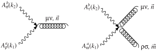
FIG. 5.: The three-point and four-point vertices. The KK states are plotted in helices.

The three-point vertex is shown in Fig. 5 and the corresponding Feynman rule is [10]

$$i{\frac{\kappa}{2}}\delta^{ab}\left[(m^{2}+k_{1}\textbf{.}k_{2})C_{\mu\nu,\rho\sigma}+D_{\mu\nu,\rho\sigma}(k_{1},k_{2})\right]\ ,$$ (A4)

where

$$C_{\mu\nu,\rho\sigma}=\eta_{\mu\rho}\eta_{\nu\sigma}+\eta_{\mu\sigma}\eta_{\nu\rho}-\eta_{\mu\nu}\eta_{\rho\sigma}$$ (A5)

is the tensor that appears in the massless graviton propagator in the de Donder gauge, and

$$D_{\mu\nu,\rho\sigma}(k_{1},k_{2})=\eta_{\mu\nu}k_{1\sigma}k_{2\rho}-\biggl{[}\eta_{\mu\sigma}k_{1\nu}k_{2\rho}+\eta_{\mu\rho}k_{1\sigma}k_{2\nu}-\eta_{\rho\sigma}k_{1\mu}k_{2\nu}+(\mu\leftrightarrow\nu)\biggr{]}\ .$$ (A6)

The Feynman rule for the four-point vertex as shown in Fig. 5 is

$$i{\frac{\kappa^{2}}{4}}\delta^{ab}\left[(m^{2}+k_{1}\textbf{.}k_{2})C_{\mu\nu,\rho\sigma\mid\omega\tau}+H_{\mu\nu\rho\sigma\omega\tau}(k_{1},k_{2})+I_{\mu\nu\rho\sigma\omega\tau}(k_{1},k_{2})\right]$$ (A7)

where

$$C_{\mu\nu,\rho\sigma\mid\omega\tau}={\frac{1}{2}}\left[\eta_{\mu\omega}C_{\rho\sigma,\nu\tau}+\eta_{\sigma\omega}C_{\mu\nu,\rho\tau}+\eta_{\rho\omega}C_{\mu\nu,\sigma\tau}+\eta_{\nu\omega}C_{\mu\tau,\rho\sigma}-\eta_{\omega\tau}C_{\mu\nu,\rho\sigma}+(\omega\leftrightarrow\tau)\right]\ ,$$ (A8)

$$H_{\mu\nu\rho\sigma\omega\tau}(k_{1},k_{2}) = -\biggl{[}C_{\mu\nu,\rho\tau}k_{1\sigma}k_{2\omega}+C_{\mu\nu,\rho\omega}k_{1\tau}k_{2\sigma}-C_{\mu\nu,\omega\tau}k_{1\rho}k_{2\sigma}+(\rho\leftrightarrow\sigma)\biggr{]}$$ (A10)

$$-\biggl{[}(\mu,\nu)\leftrightarrow(\rho,\sigma)\biggr{]}\ ,$$

and

$$~{}~{}I_{\mu\nu\rho\sigma\omega\tau}(k_{1},k_{2})=$$ (A11)

$$\Biggl{\{}\biggl{[}(C_{\sigma\omega,\nu\tau}-\eta_{\sigma\tau}\eta_{\nu\omega})k_{1\mu}k_{2\rho}+(C_{\nu\omega,\sigma\tau}-\eta_{\sigma\omega}\eta_{\nu\tau})k_{1\rho}k_{2\mu}+(\mu\leftrightarrow\nu)\biggr{]}+\left(\rho\leftrightarrow\sigma\right)\Biggr{\}}+C_{\mu\nu,\rho\sigma}k_{1\tau}k_{2\omega}\ .$$ (A12)

B

We provide details of the treatment of the infrared singularity for the case $n=2$. From the expression for the self-energy contribution from the seagull diagram, Eq. (8), we extract the integral

$$\int_{0}^{1}\,{\frac{x\,{y^{-3+{\frac{n}{2}}}}}{x+y}}\,\left(x+3\,y\right)\left(x+6\,y\right)\,dy = \left({\frac{2\,x^{2}}{n-4}}\right){}_{2}F_{1}\left[1,\,(-4+n)/2,\,(-2+n)/2,\,-1/x\right]\,$$ (B2)

$$+18\,\left({\frac{x}{n-2}}+\,{\frac{1}{n}}{}_{2}F_{1}\left[1,\,n/2,\,(2+n)/2,\,-1/x\right]\right)$$

where

$${}_{2}F_{1}\left[a,b,c,D\right]=\sum_{k=0}^{\infty}{\frac{(a)_{k}(b)_{k}}{(c)_{k}}}{\frac{D^{k}}{k!}}$$ (B3)

is the hypergeometric function and $(a)_{k}$ is the Pochhammer symbol

$$(a)_{k}=\Gamma(a+k)/\Gamma(a)\ .$$ (B4)

This result is convergent only for $n>4$. For $n=2+\epsilon$, we analytically continue the above equation and expand it in a power series in $\epsilon$,

$${\frac{16x}{\epsilon}}-x\biggl{[}x-\ln(1+x^{-1})\biggr{]}+{\cal O}(\epsilon)\ .$$ (B5)

Integrating the ${\cal O}(\epsilon^{0})$ term of the above expression over $x$, we obtain

$$-\int_{0}^{1}dx~{}x\biggl{[}x-\ln(1+x^{-1})\biggr{]}\ =\ {\frac{14}{3}}\ .$$ (B6)

We can repeat the procedure for $\Pi_{R}(0)$. The ${\cal O}(\epsilon^{0})$ term of the integral in Eq. (10) is

$$30{r^{2}}\biggl{[}Li_{2}({\frac{1}{1-r}})-Li_{2}({\frac{2}{1-r}})+Li_{2}(-r^{-1})\biggr{]}+3{r^{2}}\biggl{[}r\ln{\frac{r}{r+1}}-10\ln{\frac{2(r+1)}{r-1}}\biggr{]}$$ (B7)

$$\qquad+{3\over 2}r\left(2r-1+40\ln 2\right)-{\frac{1}{3}}\ ,$$ (B8)

where $Li_{2}$ is the dilogarithm function. The same procedure can be carried out for the integral in $\Pi_{R}(m^{2})$, but the expressions are exceedingly cumbersome and not at all illuminating. We do not show them here.

The point we wish to emphasize is that by performing dimensional regularization in the number of extra spacetime dimensions $n$, we are able to systematically isolate the infrared divergence and calculate finite quantities with a sensible physical meaning. Using the results in this Appendix, we showed that the oblique corrections vanish identically in the limit $M_{S}\rightarrow\infty$, as one would expect.

We have demonstrated this procedure only for $n=2$, but it can be carried out for any $n$. For example, for $n=3$, we would substitute $n=\epsilon+3$ and so on.

REFERENCES

- [1] T. Appelquist, A. Chodos and P.G.O. Freund (Ed.), Modern Kaluza-Klein Theories, Addison-Wesley (1987).
- [2] See e. g., M.B. Green, J.H. Schwarz and E. Witten, Superstring Theory, Cambridge University Press (1987).
- [3] I. Antoniadis, Phys. Lett. B246, 377 (1990); J. Lykken, Phys. Rev. D54, 3693 (1996); G. Shiu and S.H.H. Tye, Phys. Rev. D58, 106007 (1998).
- [4] N. Arkani-Hamed, S. Dimopoulos and G. Dvali, Phys. Lett. B429, 263 (1998); I. Antoniadis, N. Arkani-Hamed, S. Dimopoulos and G. Dvali, Phys. Lett. B436, 257 (1998).
- [5] L. Randall and R. Sundrum, Phys. Rev. Lett. 83, 3370 (1999).
- [6] N. Arkani-Hamed and M. Schmaltz, Phys. Rev. D61, 033005 (2000); N. Arkani-Hamed, L. Hall, D. Smith and N. Weiner, hep-ph/9909326; E. Mirabelli and M. Schmaltz, hep-ph/9912265.
- [7] G. Dvali and S.H.H. Tye, Phys. Lett. B450, 72 (1999); N. Kaloper and A. Linde, Phys. Rev. D59, 101303 (1999); N. Arkani-Hamed, S. Dimopoulos, N. Kaloper and J. March-Russell, hep-ph/9903224.
- [8] N. Arkani-Hamed, S. Dimopoulos and G. Dvali, Phys. Rev. D59, 086004 (1999).
- [9] G.F. Giudice, R. Rattazzi and J.D. Wells, Nucl. Phys. B544, 3 (1999).
- [10] T. Han, J.D. Lykken and R.-J. Zhang, Phys. Rev. D59, 105006 (1999).
- [11] S. Nussinov and R.E. Schrock, Phys. Rev. D59, 105002 (1999); E. A. Mirabelli, M. Perelstein and M. Peskin, Phys. Rev. Lett 82, 2236 (1999); G. Shiu, R. Shrock and S.H.H. Tye, Phys. Lett. B458, 274 (1999).
- [12] J.L. Hewett, Phys. Rev. Lett 82, 4765 (1999); T. Rizzo, Phys. Rev. D59, 115010 (1999); For a phenomenological review on virtual KK graviton signals at colliders, see T. Rizzo, hep-ph/9910255.
- [13] J. C. Long, H. W. Chan and J. C. Price, Nucl. Phys. B539, 23 (1999); and references therein.
- [14] S. Cullen and M. Perelstein, Phys. Rev. Lett 83, 268 (1999); L. Hall and D. Smith, Phys. Rev. D60, 085008 (1999); V. Barger, T. Han, C. Kao and R.-J. Zhang, Phys. Lett. B461, 34 (1999).
- [15] M. Graesser, hep-ph/9902310.
- [16] P. Das and S. Raychaudhuri, hep-ph/9908205.
- [17] M. Peskin and T. Takeuchi, Phys. Rev. Lett 65, 964 (1990); Phys. Rev. D46, 381 (1992).
- [18] M. Bando, T. Kugo, T. Noguchi and K. Yoshioka, Phys. Rev. Lett. 83, 3601 (1999); N. Arkani-Hamed, Y. Grossman and M. Schmaltz, hep-ph/9909411.
- [19] D. Kennedy and B.W. Lynn, Nucl. Phys. B322, 1 (1989).
- [20] D. Kennedy and P. Langacker, Phys. Rev. Lett 65, 2967 (1990); Phys. Rev. D44, 1591 (1992).
- [21] G. Altarelli and R. Barbieri, Phys. Lett. B253, 161 (1991); G. Altarelli, R. Barbieri and S. Jadach, Nucl. Phys. B269, 3 (1992).
- [22] W.J. Marciano and J.L. Rosner, Phys. Rev. Lett 65, 2963 (1990).
- [23] T. Takeuchi, W. Loinaz and A. Grant, hep-ph/9904207.
- [24] G. Shiu and S.-H. Tye, Phys. Rev. D58, 106007 (1998); Z. Kakushadze and S.-H. Tye, Phys. Rev. D58, 126001 (1998); I. Antoniadis, C. Bachas and E. Dudas, hep-th/9906039; L. E. Ibanez, R. Rabadan and A. M. Uranga, Nucl. Phys. B542, 112 (1999); G. Aldazabal, L. E. Ibanez and F. Quevedo, hep-th/9909172; S. Cullen, M. Perelstein and M. Peskin, hep-ph/0001166.