Enhanced Structure Function Of The Nucleon From Deep Inelastic Electron-Proton Scattering

Abstract:

The proton structure function is re-deduced from the data of deep inelastic electron-proton scattering after enhanced correction that is made due to the multiple scattering effect. The Glauber approach is used to account for the multiple scattering of electron with the quark constituents of the proton. The results are compared with the prediction of the parton model. Appreciable deviation is observed only at low values of the Bjorken scaling, which correspond to the extremely deep inelastic scattering.

1 Introduction

A dynamical understanding of quark substructure had its origin from experiments on deep inelastic lepton-nucleon scattering [1]. These showed that the complicated production of many hadrons in such a collision could be simply interpreted as quasi-elastic scattering of the lepton by point like particles or quarks. For example the linear relation between the total inelastic cross section $\sigma_{in}^{tot}(e-p)$and the center of mass energy $E$ may be explained as simple elastic scattering with point particle which depends on the coupling constant and the phase space factors. It is well known that at high momentum transfer, the elastic form factor is very small and the inelastic scattering of the incident electron is much more probable than the elastic scattering. In this case there must be an extra variable $x$ (the Bjorken scaling variable) which relates the momentum transfer $q$ to the energy transfer $\nu$ by the relation $x=\frac{q^{2}}{2M\nu}\ ,0<x<1$ . The case of $x=1$ corresponds to the elastic scattering, and it tends to zero as the reaction goes toward the deep inelastic. The differential cross section [2] is then written as,

$$\frac{d^{2}\sigma}{dq^{2}d\nu}=\frac{4\pi\alpha^{2}}{q^{4}}\frac{E^{\prime}}{E}[F_{2}(q^{2},\nu)\cos^{2}\frac{\theta}{2}+\frac{2\nu}{M}F_{1}(q^{2},\nu)\sin^{2}\frac{\theta}{2}]$$

Where the factor represents the square of the scattering amplitude of the electron by a point charged particle (the parton or quark). $F_{1}$ and $F_{2}$ are the hadron structure functions used to correct for the composite structure of the target,$E$and $E^{{}^{\prime}}$ being the incident and scattered electron energies. The factor $cos^{2}(\frac{q}{2})$stands for the square of the rotational matrix element for the electric non-spin flip part of the scattering of the electron by a charged point particle. The factor $sin^{2}(\frac{q}{2})$ is the corresponding factor for the spin-flip magnetic interaction between the magnetic moments of the electron and target particle. The problem arises now revolves about the factor $4\pi\alpha^{2}/q^{4}$ , which assumes a simple scattering of the electron by a Coulomb field of a charged point particle. And since the nucleon bag contains 3- valence quarks rather than the sea quark-antiquark pairs, so we expect multiple collision inside this bag instead of a single one. Also the presence of more than one quark in the system may make shadowing on the others during their collision. Of course these will affect the shape of the differential cross section and hence the structure functions $F_{1}$ and $F_{2}$. The present work aims to consider the effect of multiple scattering by using the Glauber [3] approach and then re-deduce the form of the structure function and compare the results with the previously published data at different regions of the Feynman variable $x$.

2 The Multiple Scattering Approach

Let us consider a bound system of three point particles (valence quarks) forming a proton as a spherical bag. The sea quark-antiquark pairs are considered as electric dipoles in their plasma phase. The problem is treated in the laboratory system in which its origin coincides with the center of the spherical bag. Assuming a collision axis in the z- direction, an incident electron with position vector and impact parameter will scatter with a momentum transfer . The scattering amplitude is given by [4],

$$f_{ms}(q)=\frac{k}{2\pi i}\int d^{2}\overline{b}\exp(i\stackrel{{\scriptstyle\_}}{{q}}.\overline{b})\left\langle\Psi\left\{s_{i}\right\}\left|\exp(i\Xi(b,\{s_{i}\})-1\right|\Psi\{s_{i}\}\right\rangle$$ (1)

Where, $k^{\prime}$ is the momentum of the scattered electron. In case of inelastic scattering, only a fraction x of the momentum of the incident electron will transfer to the quark system of the proton, leaving a momentum fraction $(1-x)$ to the scattered electron. is the total phase shift function due to all the constituent valence quarks and the associated dipoles of the system having position vectors $\{r_{i}\}$ with projections $\{s_{i}\}$ on the impact parameter plane. The suffix $i$ runs over all the flavors forming the proton bag. is the total wave function of the proton system. In Quantum Chromodynamics [5,6,7], the force between quarks is mediated by the exchange of massless spin 1, gluons, which are the carrier of the color force. When QCD is dimensionally reduces to $1+1$ dimensions [8,9,10], the gauge fields may be eliminated using their equations of motion. What remains is the effectively long-range quark-quark force, which is given by a linear two body potential [11]. This linear potential can be understood in other ways. Since gluons are massless, their propagator in momentum space is $1/q^{2}$. This is the same as the photon propagator, which corresponds to the $\frac{1}{\left|r-r^{\prime}\right|}$Coulomb potential. An appropriate wave function for the valance quarks inside the proton should satisfy certain conditions. According to the boundary condition of the problem, the quarks are considered as free particles in the central region of the nucleon and they are tightly bounded at large distance. Consequently, the nucleon space is classified into two regions. The central part, where $s<s_{i}<s_{0}$ , the quark-wave function is taken as plane wave. And in the peripheral region $s_{i}>s_{0}$, the quark wave function is approximated to harmonic oscillator wave function. Here $s_{0}$is a parameter which specifies the boundary of the central region. In the approximation of the straight line trajectories [3], the total phase shift function may be expressed as the sum of the phase shift functions due to the 3- valence quarks and N- dipoles, as scattering centers,

$$\Xi(\stackrel{{\scriptstyle\_}}{{b}},\{\stackrel{{\scriptstyle\_}}{{b}}_{i}\})=\sum_{i}\xi_{i}(\stackrel{{\scriptstyle\_}}{{b}}-\stackrel{{\scriptstyle\_}}{{b}}_{i})+\sum_{i}^{dip}\xi_{i}(\stackrel{{\scriptstyle\_}}{{b}}-\stackrel{{\scriptstyle\_}}{{b}}_{i})$$ (2)

$\qquad\xi_{i}$ is the phase shift due to the ith valence quark, and $\xi_{i}^{dip}$is the phase shift function due to the i^th electric dipole. Defining a profile function as $\Gamma(\stackrel{{\scriptstyle\_}}{{b}},\{\stackrel{{\scriptstyle\_}}{{b}}_{i}\})$,

$$\Gamma(\stackrel{{\scriptstyle\_}}{{b}},\{\stackrel{{\scriptstyle\_}}{{b}}_{i}\})=1-\exp[i\Xi(\stackrel{{\scriptstyle\_}}{{b}},\{\stackrel{{\scriptstyle\_}}{{b}}_{i}\})]$$ (3)

            

Which could be expressed in terms of the two-body profile function $\Gamma_{i}$,

$$\Gamma(\stackrel{{\scriptstyle\_}}{{b}},\{\stackrel{{\scriptstyle\_}}{{b}}_{i}\}) = 1-\prod[1-\Gamma_{i}(\stackrel{{\scriptstyle\_}}{{b}}-\stackrel{{\scriptstyle\_}}{{b}}_{i})]\prod[1-\Gamma_{i}^{dip}(\stackrel{{\scriptstyle\_}}{{b}}-\stackrel{{\scriptstyle\_}}{{b}}_{i})]$$

$$= (\sum_{j}^{3}\Gamma_{i}+\sum_{j}^{N}\Gamma_{j}^{dip})-(\sum_{j\neq i}^{3}\Gamma_{i}\Gamma_{j}+\sum_{j\neq i}\Gamma_{j}^{dip}\Gamma_{i}^{dip}+\cdot\cdot\cdot$$

$$+(-1)^{N-1}\prod_{j}^{N}\Gamma_{j}^{dip}\prod_{i}^{3}\Gamma_{i}$$

The terms of the first bracket in the R.H.S. of Eq.(2.4) represent the single scattering or the impulse approximation, the second bracket is the correction due to the binary collisions and finally the last term is the correction due to the collision with all the constituent of the proton bag, i.e. the collision at which all the three valence quarks (uud) and the N- pairs contribute the reaction. Assuming that all the quark dipoles are similar and equally probable, then Eq. (2.4) becomes,

$$\Gamma(\stackrel{{\scriptstyle\_}}{{b}},\{\stackrel{{\scriptstyle\_}}{{b}}_{i}\}) = (\sum_{j}^{3}\Gamma_{i}+N\Gamma^{dip})-(\sum_{j\neq i}^{3}\Gamma_{i}\Gamma_{j}+\frac{N(N-1)}{2}(\Gamma^{dip})^{2}$$

$$+\cdot\cdot\cdot+(-1)^{N-1}(\Gamma^{dip})^{N}\prod_{i}^{3}\Gamma_{i}$$

At sufficiently high energy, it is expected that the number N of created is much greater than the number of valence quarks. And if this number is linearly proportional to the center of mass energy Ecm of the reaction, then the terms of Eq. (2.6) are energy dependent, and read as,

$$\Gamma(b,\{b_{i}\})\simeq E_{cm}\Gamma^{dip}-\frac{E_{cm}(E_{cm}-1)}{2}(\Gamma^{dip})^{2}+\cdot\cdot\cdot$$ (6)

So that the first term in Eq. (2.6) is linearly dependent on $E_{cm}$ while the second term that represents the double scattering is quadratically dependent. This term is not important even at high energy, since the electromagnetic fine structure constant $\alpha$ appears of second order through the profile function that depresses the term as a whole. The result of Eq.(2.6) is very important, since it explains clearly the linear proportionality of the e-p total cross-section with the center of mass energy.

The problem now is reduced to the two-body collision, in other words, we have to formulate, only, for the simple two-body function and in terms of the scattering potential,

$$\Gamma_{j}(\stackrel{{\scriptstyle\_}}{{b}}-\stackrel{{\scriptstyle\_}}{{b}}_{j})=1-\exp[-\frac{i}{2k(1-x)}\int_{-\infty}^{\infty}U(\stackrel{{\scriptstyle\_}}{{b}}-\stackrel{{\scriptstyle\_}}{{b}}_{j},\stackrel{{\scriptstyle\_}}{{z}})dz]$$ (7)

Assuming a Coulomb like potential field with the form,

$$U=\frac{U_{0}}{r}\exp(-\alpha r){\qquad and\quad}\stackrel{{\scriptstyle\_}}{{r}}=(\stackrel{{\scriptstyle\_}}{{b}}-\stackrel{{\scriptstyle\_}}{{b}}_{j})+\stackrel{{\scriptstyle\_}}{{z}}$$ (8)

$$\Gamma_{j}(\stackrel{{\scriptstyle\_}}{{b}}-\stackrel{{\scriptstyle\_}}{{b}}_{j})=1-\exp[\frac{iU_{0}}{2k(1-x)}K_{o}(\alpha(b^{2}+b_{j}^{2}-2bb_{j}\cos\phi_{j}))]$$ (9)

$K_{o}(b^{2}+b_{j}^{2}-2bb_{j}\cos\phi_{j})$ is the modified Bessel function or the so called Mc-Donald function of order zero. $U_{o}$, being the strength of the field. For the two flavors u and d of the valence quarks having fractional charges $2/3$ and $-1/2$ respectively, we get

$$\Gamma_{u}(\stackrel{{\scriptstyle\_}}{{b}}-\stackrel{{\scriptstyle\_}}{{b}}_{j})=1-\exp[-\frac{iU_{0}}{2k(1-x)}K_{o}(\frac{2}{3}\alpha(b^{2}+b_{j}^{2}-2bb_{j}\cos\phi_{j}))]$$ (10)

And

$$\Gamma_{d}(\stackrel{{\scriptstyle\_}}{{b}}-\stackrel{{\scriptstyle\_}}{{b}}_{j})=1-\exp[-\frac{iU_{0}}{2k(1-x)}K_{o}(-\frac{1}{2}\alpha(b^{2}+b_{j}^{2}-2bb_{j}\cos\phi_{j}))]$$ (11)

To calculate the profile function $\Gamma_{j}^{dip}(\stackrel{{\scriptstyle\_}}{{b}}-\stackrel{{\scriptstyle\_}}{{b}}_{j})$due to the scattering from a single dipole, let us consider that a distance $\stackrel{{\scriptstyle\_}}{{\ell}}$ separates the two quarks of the dipole. The potential field due to the dipole is given by,

$$U_{dip}=-\frac{\lambda}{\ \left|\stackrel{{\scriptstyle\_}}{{r}}-\stackrel{{\scriptstyle\_}}{{r}}_{dip}+\stackrel{{\scriptstyle\_}}{{\ell}}/2\right|}+\frac{\lambda}{\ \left|\stackrel{{\scriptstyle\_}}{{r}}-\stackrel{{\scriptstyle\_}}{{r}}_{dip}-\stackrel{{\scriptstyle\_}}{{\ell}}/2\right|}$$ (12)

And putting, $\stackrel{{\scriptstyle\_}}{{r}}=\stackrel{{\scriptstyle\_}}{{b}}+\stackrel{{\scriptstyle\_}}{{z}}$, $\stackrel{{\scriptstyle\_}}{{r_{dip}}}=\stackrel{{\scriptstyle\_}}{{b_{dip}}}+\stackrel{{\scriptstyle\_}}{{z}}$ , $\stackrel{{\scriptstyle\_}}{{\ell}}=\stackrel{{\scriptstyle\_}}{{b_{\ell}}}+\stackrel{{\scriptstyle\_}}{{z}}$ where $\stackrel{{\scriptstyle\_}}{{z}}$ is the projection along the collision axis and b is the projection in the impact parameter plane. So that the phase shift function due to a dipole is,

$$\Xi^{dip}(b,b_{dip},\ell)=\frac{\lambda}{(k(1-x)}\log[\frac{(\stackrel{{\scriptstyle\_}}{{b}}-\stackrel{{\scriptstyle\_}}{{d}}_{dip}+0.5\stackrel{{\scriptstyle\_}}{{b_{\ell}}})^{2}}{(\stackrel{{\scriptstyle\_}}{{b}}-\stackrel{{\scriptstyle\_}}{{d}}_{dip}-0.5\stackrel{{\scriptstyle\_}}{{b_{\ell}}})^{2}}]$$ (13)

and the total phase shift due to the N-dipoles is,

$$\Xi_{tot}^{dip}(b,b_{dip},\ell)=\frac{\lambda}{(k(1-x)}\sum_{j}^{N}\log[\frac{(\stackrel{{\scriptstyle\_}}{{b}}-\stackrel{{\scriptstyle\_}}{{b}}_{j}+0.5\stackrel{{\scriptstyle\_}}{{b_{\ell}}})^{2}}{(\stackrel{{\scriptstyle\_}}{{b}}-\stackrel{{\scriptstyle\_}}{{b}}_{j}-0.5\stackrel{{\scriptstyle\_}}{{b_{\ell}}})^{2}}]$$ (14)

Then Eq.(2.1) becomes,

$$f_{ms}(q,x)=\frac{ik(1-x)}{2\pi}\int d^{2}\stackrel{{\scriptstyle\_}}{{b}}\exp(i\stackrel{{\scriptstyle\_}}{{q}}\cdot\stackrel{{\scriptstyle\_}}{{b}})\left\langle\Psi\{\stackrel{{\scriptstyle\_}}{{s}}_{i}\}\left|\Gamma(\stackrel{{\scriptstyle\_}}{{b}},\{\stackrel{{\scriptstyle\_}}{{s}}_{i}\}\right|\Psi\{\stackrel{{\scriptstyle\_}}{{s}}_{i}\}\right\rangle$$ (15)

3 Results and Discussion

The model predictions are tested with the experimental data of SLAC-E-049, SLAC-E-061, and SLAC-E-089 [12] that concerns the deep inelastic scattering in the lab momentum ranges {3.748 - 24.503}. A spherical proton bag is assumed with root mean square radius $R_{rms}=1.2$ $fm$. Since the quarks are almost considered independent, then the proton spatial wave function is taken as, $\Psi_{p}=\prod_{u,u,d}\Phi_{i}$ , with $\Phi_{i}$ as a plane wave for $s<s_{o}$ and $\Phi_{i}$ is a harmonic oscillator wave function for $s>s_{o}$. The parameter $s_{o}$ is adjusted to fit with the $e-p$ inelastic cross-section at the corresponding center of mass energy. It is found that $s_{o}$ is $\frac{1}{3}R_{rms}$ at the considered energy. The total profile function of the e-p scattering is calculated with a weight factor corresponding to the quark probability density inside the proton bag.

Fig.(1) shows the individual terms of the average profile function corresponding to the single, double and the triple scattering. Of course the first term is the most important one allover the impact parameter range. The double scattering term represents about 0.02 from the first one at the central region. This ratio is greater than the reciprocal of the fine structure constant $\frac{1}{137}$. The central region is populated with high density of states, so there will be a good chance for the double collision to occur. The values of the triple scattering may be neglected. In other words, the shadowing has significant effect only up to the double scattering. The resultant profile function is plotted in Fig.(2), which shows slow decrease with the impact parameter $b$, reflecting the Coulomb behavior of the assumed scattering potential. The ratio of the imaginary to the real part of the profile function is an important coefficient. It is just a measure of the degree of inelasticity of the reaction. As demonstrated in Fig.(3), the imaginary to the real part of the coefficient shows that the central region is characterized by the inelastic scattering. The inelasticity decreases with the impact parameter i.e. toward the peripheral region. The total differential cross-section is calculated according to Eq.(2.15) at $x=0.5$, and incident energy $14GeV$. The prediction of the multiple scattering model, Fig.(4) shows a large peak at small values of $q^{2}$, followed by several humps of successively decreasing height. The dashed line represents the $1/q^{4}$ behavior of the point particle scattering. It seems to tangents the humps of the multiple scattering model. It is expected that the two curves coincide at low energies where the electron wavelength is long enough and cannot probe the microscopic structure of the proton. Now replacing the factor $1/q^{4}$ that appears in Eq.(1.1) by the corresponding multiple scattering form $\left|f_{ms}\right|^{2}$, as in Eq.(2.15), and then recalculate the enhanced structure function $F_{2}^{Enh}$. Fig.(5-7) show the model prediction at $x=0.08,0.125$ and $0.55$ respectively, compared with the prediction of the parton model $F_{2}$ [13,14]. Appreciable deviation is observed at small values of $x$, which correspond to most deep inelastic scattering. As $x$ increases, the two models come closer, where the reaction is directed toward the peripheral region that is characterized by single collisions only. In spite of the observed variation in the structure function with $q^{2}$, but it still keeps its own characteristics. In other words, it leads to the half spin value of quarks forming the protons and also it doesn’t conflict with the values of their fractional charge.

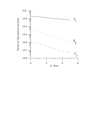
Figure 1: The first three terms of the profile function for the e-p multiple scattering. The impulse approximation, binary collision and the third order term.

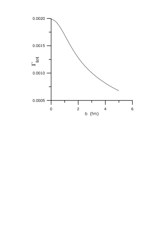
Figure 2: The total profile function of the Coulomb field due to the interaction of the incident electron with the 3-valance quarks forming the target proton.

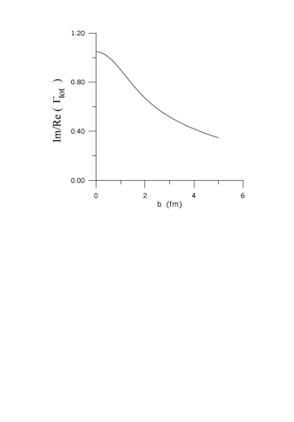
Figure 3: The ratio of imaginary to real part of the total profile function of the Coulomb field due to the interaction of the incident electron with the 3-valance quarks forming the target proton.

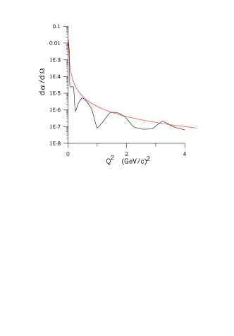
Figure 4: The differential cross section for the scattered electron in e-p experiment at 14 GeV. The black line represents the prediction of the multiple scattering model and the dotted red one is the $1/q^{4}$ law.

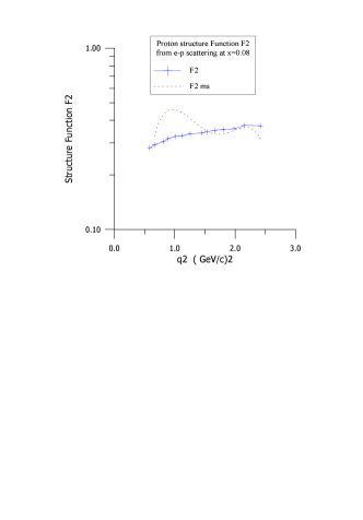
Figure 5: The proton structure function as deduced from the experiments SLAC-E-049 and SLAC-E-089 at x = 0.08. The dashed line represents the modified function due to multiple scattering.

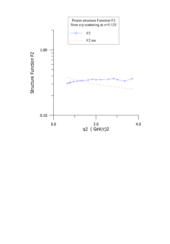
Figure 6: The proton structure function as deduced from the experiments SLAC-E-049 and SLAC-E-089 at x = 0.125. The dashed line represents the modified function due to multiple scattering.

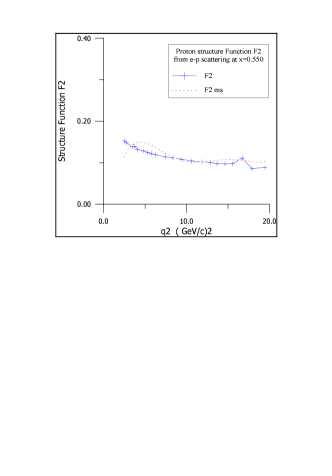
Figure 7: The proton structure function as deduced from the experiments SLAC-E-049 and SLAC-E-089 at x = 0.550. The dashed line represents the modified function due to multiple scattering.

4 Concluding Remarks.

• The multiple scattering of the electron with constituent of the proton is very important to estimate its structure function.

• The number of scattering centers inside the proton bag plays an important role to explain the linear increase of the total cross-section of the electron-proton scattering with the center of mass energy.

• Terms up to the double scattering shows significant shadowing effect during the collision.

• The square of the scattering amplitude shows a peak followed by humps of decreasing height. The asymptotic behavior of which has the form of 1/q4.

• Appreciable deviation to the structure function is due to the multiple scattering effect, particularly for the low values of the Bjorken scaling variable x which correspond to the deep inelastic scattering.

References

- [1] J. I. Friedman, Ann. Rev. Nucl. Science 22 (19972) 203.
- [2] F.E.Close, Rep. Prog. Phys. 42(1979) 1285.
- [3] M.K.Hegab, M.T.Hussein and N.M.Hassqn, Z.Phys. A336 (1990) 345.
- [4] M.T.Hussein, Proceedings of the International Cosmic Ray Conference Roma (1995). HE Session, PP. 135.
- [5] P.F.Bedaque, I.Horvath and S.G.Rajeev, Mod. Phys. Lett. A7 (1992) 3347.
- [6] G.Streman et al,Rev.Mod.Phys. 67 (1995) 157.
- [7] A.D. Martin, R.G.Roberts, W.J. Stirling and R.S. Thorne, Eur Phys. J. C4 (1998) 463.
- [8] S.G. Rajeev, Int.J.Mod. Phys. A31 (1994) 5583.
- [9] M. Gluck and E. Reys, Z. Phys. C67 (1995) 433.
- [10] S.J. Brodsky hep-ph/9807212
- [11] S.G. Rajeev and O.T. Turgut, Comm. Math. Phys. 192 (1998) 493. - P. Juan APARICIO, H. Fabian GAIOLI, and T. Edgardo GARCIA ALVAREZ, Phys. Rev. A 51, (1995) 96. - G. Krishnaswami and S. G. Rajeev, Phys. Lett. 441 (1998) 429
- [12] L.W. Whitlow, SLAC- preprint,357 (1989). - Electronic communication with the Particle Data Group (PDG) at Durham- England, for the Experiments SLAC-E-049, SLAC-E-061 and SLAC-E-089
- [13] P. E. Bosted, et al., Phys. Rev. Lett. 68 (1992) 3841.
- [14] J. Gomez, et al., Phys. Rev. D 49 (1994) 4348.