Weak-Singlet Fermions: Models and Constraints

We employ data from precision electroweak tests and collider searches to derive constraints on the possibility that weak-singlet fermions mix with the ordinary Standard Model fermions. Our findings are presented within the context of a theory with weak-singlet partners for all ordinary fermions and theories in which only third-generation fermions mix with weak singlets. In addition, we indicate how our results can be applied more widely in theories containing exotic fermions.

1 Introduction

The origins of electroweak and flavor symmetry breaking remain unknown. The Standard Model of particle physics describes both symmetry breakings in terms of the Higgs boson. Electroweak symmetry breaking occurs when the Higgs spontaneously acquires a non-zero vacuum expectation value; flavor symmetry breaking is implicit in the non-universal couplings of the Higgs to the fermions. However, the gauge hierarchy and triviality problems imply that the Standard Model is only an effective field theory, valid below some finite momentum cutoff. The true dynamics responsible for the origin of mass must therefore involve physics beyond the Standard Model. This raises the question of whether the two symmetry breakings might be driven by different mechanisms. Many theories of non-Standard physics invoke separate origins for electroweak and flavor symmetry breaking, and place flavor physics at higher energies in order to satisfy constraints from precision electroweak test and flavor-changing neutral currents.

In this paper, we explore the possibility that flavor symmetry breaking and fermion masses may be connected with the presence of weak-singlet fermions mixing with the ordinary Standard Model fermions. Specifically, we consider theories in which some of the observed fermions’ masses arise through a seesaw mechanism that results in the presence of two mass eigenstates for each affected flavor: a lighter mass eigensate whose left-handed component is predominantly weak-doublet, and a heavier one that is mostly weak-singlet. Such seesaw mass structures involving either third-generation fermions [6, 7] or all fermions [8] have played a prominent role in recent work on dynamical symmetry breaking.

This work uses published experimental data to elicit constraints on the masses and mixing strengths of the exotic fermions. We both interpret our findings within the context of several specific models and indicate where our results can be applied more widely. Our initial approach is to study Z-pole and low-energy data for signs that the known fermions include a non-Standard, weak-singlet component. Previous limits of this type [1, 2, 3] have found that the mixing fraction $\sin^{2}\theta_{mix}$ can be at most a few percent for any given fermion species. As a complementary test we also look for evidence that new heavy fermions with a large weak-singlet component are being pair-produced in high-energy collider experiments. This can provide a direct lower bound on the mass of the new fermions. Most recent limits on production of new fermions focus on sequential fermions (LH doublets and RH singlets), mirror fermions (RH doublets and LH singlets), and vector fermions (LH and RH doublets) [4]. These limits need not apply directly to weak singlet fermions, as their production cross-sections and decay paths can differ significantly from those of the other types of fermions.

We take as our benchmark a model [5] in which each ordinary fermion flavor mixes with a separate weak-singlet fermion; this allows us to consider the diverse phenomenological consequences of the singlet partners for quarks and leptons of each generation. The low-energy spectrum is completely specified, so that it is possible to calculate branching ratios and precision effects. Electroweak symmetry breaking is caused by a scalar, $\Phi$, with flavor-symmetric couplings to the fermions. Flavor symmetry breaking arises from physics at higher scales that manifests itself at low energies in the form of soft symmetry-breaking mass terms linking ordinary and weak-singlet fermions. The fermions’ chiral symmetries enforce a GIM mechanism and ensure that the flavor structure is preserved under renormalization. Due to recent interest in using weak singlets to explain the mass of the top quark [6], we also analyze variants of our benchmark model in which only the third-generation fermions have weak-singlet partners. Furthermore, we indicate how our results can be applied to other theories with weak-singlet fermions.

Since our benchmark model includes a scalar boson, it should be considered as the low-energy effective theory of a more complete dynamical model; specifically, at some finite energy scale, the scalar $\Phi$, like the Higgs boson of the Standard Model, would reveal itself to be composite. That more complete model would be akin to dynamical top seesaw models [6, 7, 8], which include composite scalars, formed by new strong interactions among quarks, and also have top and bottom quarks’ masses created or enhanced by mixing with weak-singlet states. Those particular top seesaw models generally have multiple composite scalars when more than one fermion has a weak-singlet partner; these tend to be heavier than the single scalar in our models. Moreover, in the “flavor-universal” versions [8] generation-symmetry-breaking masses for the weak singlet fermions are the source of the differences between the masses of, say, the up and top quarks; the flavor structure of our models is different. Despite these differences, most of our phenomenological results are relevant to the top seesaw models.

In the next section, we review the structure of our benchmark model, focusing on the masses, mixings, and couplings of the fermions. Section 3 discusses our fit to precision electroweak data [9] and the resulting general limits on the mixing angles between ordinary and weak-singlet fermions. We then use the constraints on mixing angles to find lower bounds on the masses of the new heavy fermion eigenstates. Section 5 discusses the new fermions’ decay modes and extracts lower bounds on the fermion masses from LEP II [10, 11] and Tevatron [12, 13] data. Oblique corrections are discussed in section 6 and our conclusions are summarized in the final section.

2 The Model

At experimentally accessible energies, the models we consider have the gauge group of the Standard Model: $SU(3)_{C}\times SU(2)_{W}\times U(1)_{Y}$. The gauge eigenstate fermions include three generations of ordinary quarks and leptons, which are left-handed weak doublets and right-handed weak singlets

$$\psi_{L} = {U\choose D}_{L},\ \ \ \ U_{R},\ \ D_{R}\ \ \ \ \ \ \ U\equiv(u,c,t),\ \ D\equiv(d,s,b)\ ,$$

$$L_{L} = {\nu_{\ell}\choose\ell}_{L},\ \ \ \ \ \ell_{R}\ \ \ \ \ \ \ \ \ \ \ \ \ \ \ \ \ell\equiv(e,\mu,\tau)\ .$$ (2.1)

In our general, benchmark model to each ‘ordinary’ charged fermion there corresponds a ‘primed’ weak-singlet fermion with the same electric charge

$$U^{\prime}_{L,R},\ \ D^{\prime}_{L,R},\ \ \ell^{\prime}_{L,R}\ .$$ (2.2)

We will also discuss the phenomenology of more specialized models in which only third-generation fermions have ‘primed’ weak-singlet partners.

The gauge symmetry allows bare mass terms for the weak-singlet fermions

$$M_{U}\bar{U}^{\prime}_{L}U^{\prime}_{R}+M_{D}\bar{D}^{\prime}_{L}D^{\prime}_{R}+M_{\ell}\bar{\ell}^{\prime}_{L}\ell^{\prime}_{R}$$ (2.3)

and we take each of these mass matrices $M_{f}$ to be proportional to the identity matrix.

The model includes a scalar doublet field

$$\Phi={\Phi^{+}\choose\Phi^{0}}$$ (2.4)

whose VEV breaks the electroweak symmetry. This scalar has Yukawa couplings that link left-handed ordinary to right-handed primed fermionic gauge eigenstates

$$\lambda_{U}\bar{\psi}_{L}\tilde{\Phi}\thinspace U^{\prime}_{R}+\lambda_{D}\bar{\psi}_{L}\Phi\thinspace D^{\prime}_{R}+\lambda_{\ell}\bar{L}_{L}\Phi\thinspace\ell^{\prime}_{R}\ .$$ (2.5)

The coupling matrices $\lambda_{f}$ are taken to be proportional to the identity matrix. The mass of the scalar is assumed to be small enough that the scalar’s contributions will prevent unitarity violation in scattering of longitudinal weak vector bosons.

Finally, there are mass terms connecting left-handed primed and right-handed ordinary fermions

$$\bar{U}^{\prime}_{L}\hbox{\bf\sf m}_{U}U_{R}+\bar{D}^{\prime}_{L}\hbox{\bf\sf m}_{D}D_{R}+\bar{\ell}^{\prime}_{L}\hbox{\bf\sf m}_{\ell}\ell_{R}.$$ (2.6)

which break the fermions’ flavor symmetries. We shall require the flavor-symmetry violation to be small: any mass $\hbox{\bf\sf m}_{f}$ should be no greater than the corresponding mass $M_{f}$. This allows our model to incorporate the wide range of observed fermion masses without jeopardizing universality [5].

As discussed in reference [5], this flavor structure is stable under renormalization. On the one hand, the flavor-symmetry-breaking mass terms (2.6) are dimension-three and cannot renormalize the flavor-symmetric dimension-four Yukawa terms (2.5). On the other, because all dimension-four terms (including the Yukawa couplings (2.5)) respect the full set of global chiral symmetries,

$$SU(3)_{\psi_{L},U^{\prime}_{R},D^{\prime}_{R}}\!\! \times SU(3)_{U^{\prime}_{L}}\times SU(3)_{D^{\prime}_{L}}\times SU(3)_{U_{R}}\times SU(3)_{D_{R}}\times$$ (2.7)

$$SU(3)_{L_{L},l^{\prime}_{R}}\times SU(3)_{l^{\prime}_{L}}\times SU(3)_{l_{R}}$$

they do not mix the mass terms (2.3) and (2.6) which break those symmetries differently. Furthermore, the global symmetries of this model lead to a viable pattern of inter-generational mixing among the fermions. Including the $M_{f}$ terms (2.3) breaks the flavor symmetries to a form

$$SU(3)_{\psi_{L},U^{\prime},D^{\prime}}\times SU(3)_{U_{R}}\times SU(3)_{D_{R}}\times SU(3)_{L_{L},l^{\prime}}\times SU(3)_{l_{R}}$$ (2.8)

nearly identical to that of the Standard Model with massless fermions. Once the flavor-symmetry-breaking masses of equation (2.6) are added, the quarks’ flavor symmetries are completely broken, leading to the presence of a CKM-type quark mixing matrix and an associated GIM mechanism that suppresses flavor-changing neutral currents. The lepton sector retains the $U(1)$’s corresponding to conservation of three separate lepton numbers.

The ordinary and primed fermions mix to form mass eigenstates; for each type of charged fermion ($f\equiv$ $U$, $D$, $\ell$) the mass matrix in the gauge basis is of the form

$$\left(\bar{f}\ \bar{f}^{\prime}\right)_{L}\ \ \left(\matrix{0&v\lambda_{f}\cr\hbox{\bf\sf m}_{f}&M_{f}\cr}\right)\ {f\choose f^{\prime}}_{R}\ .$$ (2.9)

This is diagonalized by performing separate rotations on the left-handed and right-handed fermion fields. The phenomenological issues we shall examine will depend almost exclusively on the mixing among the left-handed fermions. Hence, our discussion related to fermion mixing and its effects will focus on the left-handed fermion fields. For brevity, we omit “left” subscripts on the left-handed mixing angles and fields; we include “right” subscripts in the few instances where the right-handed mixings play a role.

To evaluate the degree of mixing among the left-handed weak-doublet and weak-singlet fields, we diagonalize the mass-squared matrix $(M^{\dagger}M)$. The rotation angle among left-handed fermions is given by

$$\sin^{2}\phi_{f}=1-{B^{2}\over{2A^{2}+2B^{2}-2A\sqrt{A^{2}+B^{2}}}}\ \ \ \ \ \ \ \ \ \ B\!\! = \!\!2v\lambda_{f}M_{f}$$ (2.10)

$$A\!\! = \!\!M_{f}^{2}+\hbox{\bf\sf m}_{f}^{2}-v^{2}\lambda_{f}^{2}$$

and the mass-squared eigenvalues are

$$\Lambda_{f}^{\pm}={1\over 2}\left(M_{f}^{2}+\hbox{\bf\sf m}_{f}^{2}+v^{2}\lambda_{f}^{2}\right)\left(1\pm\sqrt{1-(4v^{2}\lambda_{f}^{2}\hbox{\bf\sf m}_{f}^{2})/(M_{f}^{2}+\hbox{\bf\sf m}_{f}^{2}+v^{2}\lambda_{f}^{2})^{2}}\right).$$ (2.11)

Due to the matrix’s seesaw structure, one mass eigenstate ($f^{L}$) has a relatively small mass, while the mass of the other eigenstate ($f^{H}$) is far larger. The lighter eigenstate, which has a left-handed component dominated by the ordinary weak-doublet state,

$$f^{L}=\cos\phi_{f}f-\sin\phi_{f}f^{\prime}\ ,$$ (2.12)

corresponds to one of the fermions already observed by experiment. Its mass is approximately given by (for $v\lambda_{f}<M_{f}$ and $\hbox{\bf\sf m}_{f}\leq M_{f}$)

$$(m_{f}^{L})^{2}\approx{(v\lambda_{f}\hbox{\bf\sf m}_{f})^{2}\over M_{f}^{2}+(v\lambda_{f})^{2}+\hbox{\bf\sf m}_{f}^{2}}\ .$$ (2.13)

The heavier eigenstate, whose left-handed component is largely weak-singlet,

$$f^{H}=\sin\phi_{f}f+\cos\phi_{f}f^{\prime}$$ (2.14)

has a mass of order

$$(m_{f}^{H})^{2}\approx M_{f}^{2}+(v\lambda_{f})^{2}+\hbox{\bf\sf m}_{f}^{2}-(m_{f}^{L})^{2}\ .$$ (2.15)

The interactions of the mass eigenstates with the weak gauge bosons differ from those in the Standard Model because the primed fermions lack weak charge. The coupling of $f^{L}$ ($f^{H}$) to the W boson is proportional to $\cos\phi_{f}$ ($\sin\phi_{f})$; the right-handed states are purely weak-singlet and do not couple to the $W$ boson. Thus the couplings of left-handed leptons to the $W$ boson look like (since we neglect neutrino mixing)

$${\frac{ie}{\sin\theta_{W}}}\,\left(\ell^{L}\gamma_{\mu}\bar{\nu_{\ell}}\cos{\phi_{\ell}}+\ell^{H}\gamma_{\mu}\bar{\nu_{\ell}}\sin{\phi_{\ell}}\right)W^{\mu}$$ (2.16)

When weak-singlet partners exist for all three generations of quarks, the left-handed quarks’ coupling to the $W$ bosons is of the form

$${\frac{ie}{\sin\theta_{W}}}\,(\bar{U^{L}},\bar{U^{H}})\gamma_{\mu}V_{UD}\left(\begin{array}[]{c}D^{L}\\ D^{H}\end{array}\right)W^{\mu}$$ (2.17)

The $6\times 6$ non-unitary matrix $V_{UD}$ is related to the underlying $3\times 3$ unitary matrix $A_{UD}$ that mixes quarks of different generations

$$V_{UD}=\left(\begin{array}[]{cc}C_{U}\ A_{UD}\ C_{D}&\ \ -C_{U}\ A_{UD}\ S_{D}\\ -S_{U}\ A_{UD}\ C_{D}&\ \ S_{U}\ A_{UD}\ S_{D}\\ \end{array}\right)$$ (2.18)

through diagonal matrices of mixing factors

$$C_{U}\equiv diag(\cos{\phi_{u}},\,\cos{\phi_{c}},\,\cos{\phi_{t}})\,,\ \ \ \ C_{D}\equiv diag(\cos{\phi_{d}},\,\cos{\phi_{s}},\,\cos{\phi_{b}})\,,$$

$$S_{U}\equiv diag(\sin{\phi_{u}},\,\sin{\phi_{c}},\,\sin{\phi_{t}})\,,\ \ \ \ S_{D}\equiv diag(\sin{\phi_{d}},\,\sin{\phi_{s}},\,\sin{\phi_{b}})\,.$$

The unitary mixing matrix $A_{UD}$, like the CKM matrix in the Standard Model, is characterized by three real angles and one CP-violating phase. But it is the elements of $V_{UD}$ which are directly accessible to experiment. While $V_{UD}$ is non-unitary, any two columns (or rows) are still orthogonal.

The coupling of left-handed mass-eigenstate fermions to the $Z$ boson is of the form

$${\frac{ie}{\sin\theta_{W}\cos\theta_{W}}}\,(\bar{f^{L}},\bar{f^{H}})\gamma_{\mu}\left(\begin{array}[]{cc}\cos^{2}{\phi_{f}}T_{3}-Q\sin^{2}{\theta_{W}}&\cos{\phi_{f}}\sin{\phi_{f}}T_{3}\\ \cos{\phi_{f}}\sin{\phi_{f}}T_{3}&\sin^{2}\phi_{f}T_{3}-Q\sin^{2}\theta_{W}\end{array}\right)\left(\begin{array}[]{c}f^{L}\\ f^{H}\end{array}\right)Z^{\mu}$$ (2.19)

where $T_{3}$ and $Q$ are the weak and electromagnetic charges of the ordinary fermion. The right-handed states, being weak singlets, couple to the $Z$ exactly as Standard Model right-handed fermions would.

The scalar boson $\Phi$ couples to the mass-eigenstate fermions according to the Lagrangian term

$${\lambda_{f}}\,(\bar{f^{L}},\bar{f^{H}})_{left}\left(\begin{array}[]{cc}-\cos{\phi_{f}}\,\sin{\phi_{f,right}}&\cos{\phi_{f}}\,\cos{\phi_{f,right}}\\ -\sin{\phi_{f}}\,\sin{\phi_{f,right}}&\sin{\phi_{f}}\,\cos{\phi_{f,right}}\end{array}\right)\left(\begin{array}[]{c}f^{L}\\ f^{H}\end{array}\right)_{right}\Phi\ \ \ +\ h.c.$$ (2.20)

where $\phi_{f,right}$ is the mixing angle for right-handed fermions.

A few notes about neutral-current physics are in order. Flavor-conserving neutral-current decays of the heavy states into light ones are possible (e.g. $\mu^{H}\to\mu^{L}\nu_{\mu}\bar{\nu}_{\mu}$). This affects the branching ratios in heavy fermion decays and will be important in discussing searches for the heavy states in Section 5. Flavor-changing neutral (FCNC) processes are absent at tree-level and highly-suppressed at higher order in the benchmark model, due to the GIM mechanism mentioned earlier. For example, we have evaluated the fractional shift in the predicted value of $\Gamma(b\to s\gamma)$ by adapting the results in [3]. As we shall see in sections 3 and 4, electroweak data already constrain the mixings between ordinary and singlet fermions to be small and the masses of the heavy up-type fermion eigenstates to be large (so that the Wilson coefficients $c_{7}(m_{f})$ that enter the calculation of $\Gamma(b\to s\gamma)$ are all in the high-mass asymptotic regime). The shift in $\Gamma(b\to s\gamma)$ is therefore at most a few percent, which is well within the 10% - 30% uncertainty of the Standard Model theoretical predictions [14] and experimental observations [15].

3 General limits on mixing angles

Precision electroweak measurements constrain the degree to which the observed fermions can contain an admixture of weak-singlet exotic fermions. The mixing alters the couplings of the light fermions to the $W$ and $Z$ from their Standard Model values, as discussed above, and the shift in couplings alters the predicted values of many observables. Using the general approach of reference [16], we have calculated how inclusion of mixing affects the electroweak observables listed in Table 1. The resulting expressions for these leading (tree-level) alterations are given in the Appendix as functions of the mixing angles. We then performed a global fit to the electroweak precision data to constrain the mixing angles between singlet and ordinary fermions. The experimental values of the observables used in the fit and their predicted values in the Standard Model are listed in Table 1.

To begin, we considered the benchmark scenario (called Case A, hereafter) in which all electrically charged fermions have weak-singlet partners [5]. All of the electroweak observables given in Table 1 receive corrections from fermion mixings in this case. We performed a global fit for the values of the 8 mixing angles of the fermions light enough to be produced at the Z-pole: the 3 leptons, 3 down-type quarks and 2 up-type quarks. At 95% (90%) confidence level, we obtain the following upper bounds on the mixing angles:

$$\sin^{2}\phi_{e}\leq 0.0024\,\,(0.0020)\,,\ \ \ \ \sin^{2}\phi_{\mu}\!\! \leq \!\!0.0030\,\,(0.0026)\,,\ \ \sin^{2}\phi\tau\leq 0.0030\,\,(0.0025)$$

$$\sin^{2}\phi_{d}\leq 0.015\,\,(0.013)\,,\ \ \ \ \ \ \ \sin^{2}\phi_{s}\!\! \leq \!\!0.015\,\,(0.011)\,,\ \ \ \ \ \sin^{2}\phi_{b}\leq 0.0025\,\,(0.0019)$$

$$\sin^{2}\phi_{u}\leq 0.013\,\,(0.011)\,,\ \ \ \ \ \ \ \sin^{2}\phi_{c}\!\! \leq \!\!0.020\,\,(0.017)\,.\$$ (3.1)

The 90% c.l. limits are included to allow comparison with the slightly weaker limits resulting from the similar analysis of earlier data in reference [2].

The limits on the mixing angles are correlated to some degree. For example, most observables that are sensitive to $d$ or $s$ quark mixing depend on $\sin^{2}\phi_{d}+\sin^{2}\phi_{s}$. Indeed, repeating the global fit using the linear combinations $(\sin^{2}\phi_{d}\pm\sin^{2}\phi_{s})/2$ yields a slightly stronger limit for the sum $(\sin^{2}\phi_{d}+\sin^{2}\phi_{s})/2\leq.0094$ and a slightly looser one for the difference $-0.0071<(\sin^{2}\phi_{d}-\sin^{2}\phi_{s})/2\leq.0195$. This turns out not to affect our use of the mixing angles to set mass limits in the next section of the paper: limits on the $d^{H}$ and $s^{H}$ masses arise from the more tightly-constrained $b$-quark mixing factor $\sin^{2}\phi_{b}$ instead.

Quantity	Experiment	SM	Reference
$\Gamma_{Z}$	2.4939 $\pm$ 0.0024	2.4958	[9]
$\sigma_{h}$	41.491 $\pm$ 0.058	41.473	[9]
$A_{\tau}(P_{\tau})$	0.1431 $\pm$ 0.0045	0.1467	[9]
$A_{e}(P_{\tau})$	0.1479 $\pm$ 0.0051	0.1467	[9]
$A_{LR}$	0.1550 $\pm$ 0.0034	0.1467	[4] (ref. 59)
$R_{b}$	0.21656 $\pm$ 0.00074	0.21590	[9]
$R_{c}$	0.1735 $\pm$ 0.0044	0.1722	[9]
$A_{FB}^{b}$	0.0990 $\pm$ 0.0021	0.1028	[9]
$A_{FB}^{c}$	0.0709 $\pm$ 0.0044	0.0734	[9]
${\cal{A}}_{b}$	0.867 $\pm$ 0.035	0.935	[9]
${\cal{A}}_{c}$	0.647 $\pm$ 0.040	0.668	[9]
$Q_{W}(Cs)$	-72.41 $\pm$.25 $\pm$ .80	-73.12 $\pm$ .06	[4] (refs. 48, 49)
$Q_{W}(Tl)$	-114.8 $\pm$ 1.2 $\pm$ 3.4	-116.7 $\pm$ .1	[4] (refs. 48, 49)
$R_{e}$	20.783 $\pm$ 0.052	20.748	[9]
$R_{\mu}$	20.789 $\pm$ 0.034	20.748	[9]
$R_{\tau}$	20.764 $\pm$ 0.045	20.748	[9]
$A_{FB}^{e}$	0.0153 $\pm$ 0.0025	0.01613	[9]
$A_{FB}^{\mu}$	0.0164 $\pm$ 0.0013	0.01613	[9]
$A_{FB}^{\tau}$	0.0183 $\pm$ 0.0017	0.01613	[9]
$A_{FB}^{s}$	0.118 $\pm$ 0.018	0.1031 $\pm$.0009	[4]
$M_{W}$	80.39 $\pm$ 0.06	80.38	[17]
$g_{eV}(\nu e\rightarrow\nu e)$	-0.041$\pm$ 0.015	-0.0395$\pm$.0005	[4]
$g_{eA}(\nu e\rightarrow\nu e)$	-0.507 $\pm$ 0.014	-0.5064$\pm$.0002	[4]
$g_{L}^{2}(\nu N\rightarrow\nu X)$	0.3009$\pm$0.0028	0.3040 $\pm$ .0003	[4]
$g_{R}^{2}(\nu N\rightarrow\nu X)$	0.0328 $\pm$ 0.0030	0.0300	[4]
$R_{\pi}$	(1.230 $\pm$ .004)$\times 10^{-4}$	(1.2352 $\pm$ .0005)$\times 10^{-4}$	[4], [18]
$R_{\tau}$	(1.347 $\pm$ .0082)$\times 10^{6}$	1.343 $\times 10^{6}$	[4], [19]
$R_{\mu\tau}$	(1.312 $\pm$ .0087)$\times 10^{6}$	1.304 $\times 10^{6}$	[4], [19]

Table 1: Data used in fits to constrain mixing angles: experimentally measured electroweak observables and their values within the Standard Model.

We, similarly, placed limits on the relevant mixing angles for three scenarios in which only third-generation fermions have weak-singlet partners. In Case B where the top quark, bottom quark and tau lepton have partners, the 12 sensitive observables are $\Gamma_{Z},\sigma_{h},R_{b,\,c,\,e,\,\mu,\,\tau},A_{FB}^{b,\tau},{\cal{A}}_{b},$ and $R_{e\tau,\mu\tau}$. The resulting 95% (90%) confidence level limits on the bottom and tau mixing angles are

$$\sin^{2}\phi_{\tau}\leq 0.0018\,\,(0.0014)\,,\ \ \ \ \ \sin^{2}\phi_{b}\leq 0.0013\,\,(0.00084)$$ (3.2)

In Case C, where only the top and bottom quarks have partners, the nine affected quantities are $\Gamma_{Z},\sigma_{h},R_{b,\,c,\,e,\,\mu,\,\tau},A_{FB}^{b},$ and ${\cal{A}}_{b}$. The sole constraint is

$$\sin^{2}\phi_{b}\leq\,0.0013\,\,(0.00084)$$ (3.3)

In Case D, where only the tau leptons have partners, only the six quantities $\Gamma_{Z},\sigma_{h},$ $R_{\tau},A_{FB}^{\tau},$ and $R_{e\tau,\mu\tau}$ are sensitive, and the limit on the tau mixing angle is

$$\sin^{2}\phi_{\tau}\leq 0.0020\,\,(0.0016)$$ (3.4)

These upper bounds on the mixing angles depend only on which fermions have weak partners, and not on other model-specific details. They apply broadly to theories in which the low-energy spectrum is that of the Standard Model plus weak-singlet fermions.

4 From mixing angles to mass limits

The constraints on the mixing between the ordinary and exotic fermions imply specific lower bounds on the masses of the heavy fermion mass eigenstates (2.15). We will extract mass limits from mixing angle limits first in the general case [5] in which all charged fermions have singlet partners, and then in scenarios where only the third generation fermions do.

4.1 Case A: all generations mix with singlets

Because the heavy fermion masses $m_{f}^{H}$ depend on $v\lambda_{f}$, $M_{f}$, and $\hbox{\bf\sf m}_{f}$, we must determine the allowed values of all three of these quantities in order to find lower bounds on the $m_{f}^{H}$. For the three fermions of a given type, (e.g. $e$, $\mu$, $\tau$), the values of $\lambda_{f}$ and $M_{f}$ are common. The different values of $m^{L}_{f}$ arise from differences among the $\hbox{\bf\sf m}_{f}$, and the form of equation (2.13) makes it clear that larger values of $\hbox{\bf\sf m}_{f}$ correspond to larger values of $m^{L}_{f}$.

How can we ensure that the third-generation fermion in the set gets a large enough mass ? If we set $\hbox{\bf\sf m}_{f}$ to the largest possible value, $\hbox{\bf\sf m}_{f}=M_{f}$, there is a minimum value of $v\lambda_{f}$ required to make $m^{L}_{f}$ large enough. A smaller value of $\hbox{\bf\sf m}_{f}$ would require a still larger value of $v\lambda_{f}$ to arrive at the same $m^{L}_{f}$. In other words, starting from (2.13), and recalling $v\lambda_{f}<M_{f}$ we find

$$v\lambda_{f}\geq\sqrt{2}m^{L}_{f3}$$ (4.1)

where “$f3$” denotes the third-generation fermion of the same type as “$f$” (e.g. if “$f$” is the electron, “$f3$” is the tau lepton). The specific limits for the three types of charged fermions are:

$$v\lambda_{\ell}\geq 2.5\ {\rm GeV},\ \ \ \ v\lambda_{D}\geq 6.0\ {\rm GeV}\ \ \ \ v\lambda_{U}\geq 247\ {\rm GeV}$$ (4.2)

Knowing this allows us to obtain a rough lower bound on the heavy fermion mass eigenstates. Since we require $M_{f}\geq v\lambda_{f}$ and since the smallest possible value of $\hbox{\bf\sf m}_{f}$ is zero, we can immediately apply (4.1) to (2.15) and find

$$(m_{f}^{H})^{2}\stackrel{{\scriptstyle>}}{{\sim}}4(m_{f3}^{2})-(m_{f}^{L})^{2}$$ (4.3)

For instance, the mass of the heavy top eigenstate must be at least

$$m_{t}^{H}\stackrel{{\scriptstyle>}}{{\sim}}\sqrt{3}m_{t}^{L}\approx 300{\rm GeV}$$ (4.4)

We can improve on these lower bounds in the following way. Because $(m_{f}^{H})^{2}$ is a monotonically increasing function of $(v\lambda)^{2}$, the minimum $v\lambda_{f}$, found above, yields the lowest possible value of $m^{H}_{f}$. Thus, if we know what value of $\hbox{\bf\sf m}_{f}$ should be used self-consistently with the smallest $v\lambda_{f}$, we can use (2.15) to obtain a more stringent lower bound on $m_{f}^{H}$. The appropriate values

$$\hbox{\bf\sf m}_{f} = M_{f}\ \ \ \ \ {\rm(3rd\ generation)}$$ (4.5)

$$\hbox{\bf\sf m}_{f} = m^{L}_{f}\sqrt{M_{f}^{2}+v^{2}\lambda_{f}^{2}\over{v^{2}\lambda_{f}^{2}-(m^{L}_{f})^{2}}}\ \ \ \ \ {\rm(1st\ or\ 2nd\ generation)}$$ (4.6)

follow from our previous discussion and from inverting equation (2.13), respectively. Because $\hbox{\bf\sf m}_{f}<<M_{f}$ for the first and second generation fermions, our previous lower bound on $m_{f}^{H}$ for those generations is not appreciably altered. For the third generation we obtain the more restrictive

$$(m_{f}^{H})^{2}\stackrel{{\scriptstyle>}}{{\sim}}5(m_{f3}^{L})^{2}$$ (4.7)

so that, for example,

$$m_{t}^{H}\stackrel{{\scriptstyle>}}{{\sim}}\sqrt{5}m_{t}^{L}\approx 390\ {\rm GeV}\ \ .$$ (4.8)

We can do still better by invoking our precision bounds on the mixing angles $\sin\phi_{f}$. Recalling $v\lambda_{f}<M_{f}$ and $\hbox{\bf\sf m}_{f}\leq M_{f}$, allows us to approximate our expression (2.10) for the mixing angle as

$$\sin\phi_{f}\approx{{v\lambda_{f}M_{f}}\over{M_{f}^{2}+\hbox{\bf\sf m}_{f}^{2}-v^{2}\lambda_{f}^{2}}}\ .$$ (4.9)

Further simplification of this relation depends on the generation to which fermion $f$ belongs. For example, among the charged leptons, $\hbox{\bf\sf m}_{e}$ and $\hbox{\bf\sf m}_{\mu}$ are far smaller than $M_{\ell}$, while $\hbox{\bf\sf m}_{\tau}$ could conceivably be of the same order as $M_{\ell}$. Thus the limits on the leptons’ mixing angles imply

$$M_{\ell}\geq{\rm Max}\left[{v\lambda_{\ell}\over{2\sin\phi_{\tau}}}\,,{v\lambda_{\ell}\over{\sin\phi_{\mu}}}\,,{v\lambda_{\ell}\over{\sin\phi_{e}}}\right]$$ (4.10)

The strongest bound on $M_{\ell}$ comes from $\sin\phi_{e}$; that for $M_{D}$, from $\sin\phi_{b}$; that for $M_{U}$, from $\sin\phi_{u}$:

$$M_{\ell}\geq{v\lambda_{\ell}\over{\sin\phi_{e}}}\geq 51\,{\rm GeV},\ \ \ \ \ \ \ M_{U}\geq{v\lambda_{U}\over{\sin\phi_{u}}}\geq 2.2\,{\rm TeV},\ \ \ \ \ \ M_{D}\geq{v\lambda_{D}\over{2\sin\phi_{b}}}\geq 60\,{\rm GeV}$$ (4.11)

Combining those stricter lower limits on $M_{f}$ with our bounds (4.1) on $v\lambda_{f}$ and our expression for the heavy fermion mass (2.15) gives us a lower bound on the $m^{H}_{f}$ for each fermion flavor. For the third generation fermions we use (4.5) for the value of $\hbox{\bf\sf m}_{f}$ and obtain the 95% c.l. lower bounds

$$m^{H}_{\tau} \geq m^{L}_{\tau}\sqrt{1+4/\sin^{2}\phi_{e}}\ \geq\ 73\ {\rm GeV}$$ (4.12)

$$m^{H}_{t} \geq m^{L}_{t}\sqrt{1+4/\sin^{2}\phi_{u}}\ \geq\ 3.1\ {\rm TeV}$$ (4.13)

$$m^{H}_{b} \geq m^{L}_{b}\sqrt{1+1/\sin^{2}\phi_{b}}\ \geq\ 86\ {\rm GeV}\ \ .$$ (4.14)

For the lighter fermions, we use equation (4.6) for the $\hbox{\bf\sf m}_{f}$. Since $\hbox{\bf\sf m}_{f}<<M_{f}$ in these cases, we find

$$m^{H}_{e},m^{H}_{\mu} \stackrel{{\scriptstyle>}}{{\sim}} m^{L}_{\tau}\sqrt{2+2/\sin^{2}\phi_{e}}\ \ \geq\ \ 51\,{\rm{GeV}}$$ (4.15)

$$m^{H}_{u},m^{H}_{c} \stackrel{{\scriptstyle>}}{{\sim}} m^{L}_{t}\sqrt{2+2/\sin^{2}\phi_{u}}\ \ \geq\ \ \ 2.2\,{\rm{TeV}}$$ (4.16)

$$m^{H}_{d},m^{H}_{s} \stackrel{{\scriptstyle>}}{{\sim}} m^{L}_{b}\sqrt{2+1/2\sin^{2}\phi_{b}}\ \ \geq\ \ \ 61\,{\rm{GeV}}\ \ .$$ (4.17)

The mass limits for the heavy leptons and down-type quarks are also represented graphically in figures 1 and 2. In figure 1, which deals with the leptons, the axes are the flavor-universal quantities $M_{\ell}$ and $v\lambda_{\ell}$. The shaded region indicates the experimentally allowed region of the parameter space. The lower edge of the allowed region is delimited by the lower bound on $v\lambda_{\ell}$ of equation (4.2), as represented by the horizontal dotted line. The left-hand edge of the allowed region is demarked by the upper bound on the electron mixing factor, $\sin^{2}\phi_{e}$, as shown by the dashed curve with that label. The form of this curve, $\sin^{2}\phi_{e}(M_{\ell},v\lambda_{\ell})=0.0024$, was obtained numerically by using equation (2.11) for $m_{e}^{L}$ to put the unknown $\hbox{\bf\sf m}_{e}$ in terms of $M_{\ell}$, $v\lambda_{\ell}$ and the observed mass of the electron ($m_{e}^{L}=.511$ MeV) and inserting the result into equation (2.10). The curves for the muon and tau mixing angles were obtained similarly, but provide weaker limits on the parameter space (as shown by the dashed curves labeled $\sin^{2}\phi_{\mu}$, and $\sin^{2}\phi_{\tau}$). The lowest allowed values of the heavy fermion masses $m_{e,\mu}^{H}$ and $m^{H}_{\tau}$ are those whose curves intersect the tip of the allowed region; these are shown by the solid curves, obtained numerically by using equation (2.11) to replace the unknown $\hbox{\bf\sf m}_{e},\hbox{\bf\sf m}_{\tau}$ by the known $m^{L}_{e},m^{L}_{\tau}$ in our expressions for $m^{H}_{e}$ and $m^{H}_{\tau}$. Figure 2 shows the analogous limits on the mixing angles and heavy-eigenstate masses for the down-type quarks.

We can also construct a plot of the allowed region of $M_{U}$ vs. $v\lambda_{U}$ parameter space. The lower edge comes from the lower bound on $v\lambda_{U}$ and the left-hand edge, from the upper bound on $\sin\phi_{u}$. We can then use the known value of $m^{L}_{t}$ to calculate the size of the top quark mixing factor $\sin^{2}\phi_{t}$ at any given point in the allowed region. Numerical evaluation reveals

$$\sin^{2}\phi_{t}\leq 0.013\,\,(0.011)$$ (4.18)

at 95% (90%) c.l. This is a limit on top quark mixing imposed by self-consistency of the model.

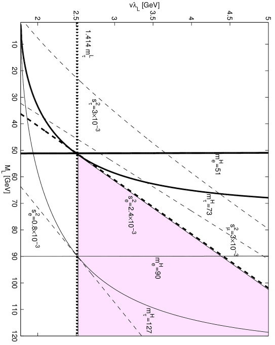
Figure 1: A graphical representation of the coupling and mass limits for the $e^{H}$ and $\tau^{H}$ states in the $M_{\ell}$ vs. $v\lambda_{\ell}$ plane. The shaded region indicates the experimentally allowed region of the parameter space. The quantities on the axes are flavor-blind; separate curves for different lepton flavors are shown. Each dashed curve shows the upper bound on $\sin^{2}\phi_{\ell}$ for one lepton and excludes the region to its left. Each solid curve shows the lower bound on $m^{H}_{\ell}$ for one lepton (the limits for $e$ and $\mu$ are identical, as discussed in the text and equation(4.15). The horizontal dotted line indicates the minimum allowed value of $v\lambda_{\ell}$ (4.1).

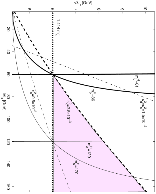
Figure 2: A graphical representation of the mass limits for the $d^{H}$ and $b^{H}$ states in the $M_{D}$ vs. $v\Lambda_{D}$ plane. The shaded region indicates the experimentally allowed region of the parameter space The quantities along the axes are flavor-blind; separate curves for different quark flavors are shown. Each dashed curve shows the upper bound on $\sin^{2}\phi_{D}$ for one quark and excludes the region to its left. Each solid curve shows the lower bound on $m^{H}_{D}$ for one quark (the limits for $d$ and $s$ are identical, as discussed in the text and equation (4.17). The horizontal dotted line indicates the minimum allowed value of $v\lambda_{D}$ (4.1).

In section 5, we will compare the mass limits just extracted from precision data with those derived from searches for direct production of new fermions at the LEP II and Tevatron colliders. The lower bounds on the masses of the heavy down-type quarks or charged leptons admit the possibility of those particles’ being produced at current experiments. The heavy up-type quarks are too massive to be even singly produced at existing colliders.

4.2 Cases B, C, and D: third-generation fermions mix with singlets

If only third-generation fermions have weak-singlet partners, there are a few differences in the analysis that yields lower bound on heavy eigenstate masses. All follow from the fact that the lower bounds on the $M_{f}$ (as in equation (4.10)) can no longer come from precision limits on the mixing angles of 1st or 2nd generation fermions (since those fermions no longer mix with weak singlets).

To obtain the precision bounds on the masses of $b^{H}$ and $\tau^{H}$, we start by writing the lower limits on $M_{\ell}$ and $M_{D}$ that come from the mixing angles:

$$M_{\ell}\geq{v\lambda_{\ell}\over{2\sin\phi_{\tau}}}\,,\ \ \ \ \ \ M_{D}\geq{v\lambda_{D}l\over{2\sin\phi_{b}}}\ \ .$$ (4.19)

The factor of 2 in the denominator arises because the mixing angles belong to a third-generation fermion (so that $\hbox{\bf\sf m}_{f}=M_{f}$). We therefore find

$$m^{H}_{\tau} \geq m^{L}_{\tau}\sqrt{1+1/\sin^{2}\phi_{\tau}}$$ (4.20)

$$m^{H}_{b} \geq m^{L}_{b}\sqrt{1+1/\sin^{2}\phi_{b}}.$$ (4.21)

In Case B where all third-generation fermions mix with weak-singlet fermions, the mixing angle limits (3.2) based on the twelve sensitive observables yield 95% c.l. lower bounds

$$m^{H}_{\tau} \geq 42\ {\rm GeV}$$ (4.22)

$$m^{H}_{b} \geq 119\ {\rm GeV}$$ (4.23)

In Case C, where only third-generation quarks have partners, (3.3) which was obtained by a fit to the nine aaffected observables, gives

$$m^{H}_{b}\geq 119\ {\rm GeV}$$ (4.24)

while in Case D, where only tau leptons have partners, (3.4) based on six affected precision electroweak quantities implies

$$m^{H}_{\tau}\geq 40\ {\rm GeV}$$ (4.25)

Compared with the limits in Case A, we see that the lower bound on $m^{H}_{b}$ is strengthened because the precision limit (3.2, 3.3) on $\sin^{2}\phi_{b}$ is more stringent. In contrast, the lower bound on $m^{H}_{\tau}$ is weakened because the bound now depends on a third-generation instead of a first-generation mixing angle: equation (4.20) is approximately $m_{\tau}^{H}\geq m^{L}_{\tau}/\sin\phi_{\tau}$ whereas equation (4.12) was roughly $m_{\tau}^{H}\geq 2m^{L}_{\tau}/\sin\phi_{e}$.

Note that in theories where the top is the only up-type quark to have a weak-singlet partner, such as Cases B and C, the only bound on $m^{H}_{t}$ comes from equation (4.8). While this is far weaker than the limit in Case A, it still ensures that the heavy top eigenstate is too massive to have been seen in existing collider experiments, even if singly produced.

5 Limits on direct production of singlet fermions

While interpreting the general mixing angle limits in terms of mass limits requires specifying an underlying model structure, it is also possible to set more general mass limits by considering searches for direct production of the new fermions. The LEP experiments have published limits on new sequential charged leptons [10][11]; the Tevatron experiments have done the same for new quarks [12][13]. In this section, we adapt the limits to apply to scenarios in which the new fermions are weak singlets rather than sequential.

5.1 Decay rates of heavy fermions

A heavy fermion decays preferentially to a light fermion plus a Z, W, or $\Phi$ boson which subsequently decays to a fermion-antifermion pair (see figure 3)

At tree-level, and neglecting final state light fermion masses, we obtain the following partial rates for vector boson decay modes of the heavy fermions

$$\!\Gamma(f^{H}_{i}\rightarrow f^{L}_{j}V) = \sum_{k,l}\Gamma(f^{H}_{i}\rightarrow f^{L}_{j}V\rightarrow f^{L}_{j}f^{L}_{k}f^{L}_{l})$$

$$= \sum_{k,l}{(c^{V}_{ij}\,c^{V}_{kl})^{2}\over{3\,\pi^{3}\,2^{8}}}\,m_{f_{i}}^{H}\,F\bigg{[}{\bigg{(}{m_{f_{i}}^{H}\over M_{V}}\bigg{)}}^{2}\,,\,{\Gamma_{V}\over M_{V}}{\bigg{]}}$$

where V represents a Z or W boson, while $\Gamma_{V}$ and $M_{V}$ are, respectively, the vector boson’s decay rate and mass. Function $F(x,y)$ is presented in appendix B. The vertex factors $c^{V}_{ij}$ ($c^{V}_{kl}$) are, as shown in figure 3, the $f^{H}_{i}f^{L}_{j}V$ ($f^{L}_{k}f^{L}_{l}V$) couplings which may be read from equations (2.16) – (2.19).

Our results for the charged-current decay mode agree with those presented in integral form in [21]. Moreover, equation yields the standard asymptotic behaviors in the limit of heavy fermion masses far above or far below the electroweak bosons’ masses (see appendix B). Since some of our heavy fermions can, instead, have masses of order 80-90 GeV, we use the full result (5.1) in our evaluation of branching fractions and search potentials.

Similarly, we find the partial rate for the scalar decay mode to be

$$\!\Gamma(f^{H}_{i}\rightarrow f^{L}_{j}\,\Phi) = \sum_{k,l}\Gamma(f^{H}_{i}\rightarrow f^{L}_{j}\,\Phi\rightarrow f^{L}_{j}f^{L}_{k}f^{L}_{l})$$

$$= \sum_{k,l}{(c^{\Phi}_{ij}\,c^{\Phi}_{kl})^{2}\over{\pi^{3}\,2^{10}}}\,m_{f_{i}}^{H}\,G\bigg{[}{\bigg{(}{m_{f_{i}}^{H}\over M_{\Phi}}\bigg{)}}^{2}\,,\,{\Gamma_{\Phi}\over M_{\Phi}}{\bigg{]}}$$

where $\Gamma_{\Phi}$ and $M_{\Phi}$ are the decay rate and the mass of the scalar boson, $\Phi$. Function $G(x,y)$ and additional details are given in appendix B. The vertex factors $c^{\Phi}_{ij}$ ($c^{\Phi}_{kl}$) are, as indicated in figure 3, the $f^{H}_{i}f^{L}_{j}\Phi$ ($f^{L}_{k}f^{L}_{l}\Phi$) couplings which may be read off of equation (2.20).

Figure 3: Scalar ($\Phi$) and weak boson (V $\equiv$ Z or W) decay modes of a heavy fermion ($f^{H}$).

We have numerically evaluated the couplings of the light fermions to the scalar, Z, and W as functions of the $M_{f}$ and the $v\lambda_{f}$. In the region of the model parameter space that is allowed by precision electroweak measurements, we find that these couplings are within 1% of their Standard Model values. Therefore, in this section of the paper, we approximate the $\Phi ff$ and $Vff$ couplings for the light fermions by the Standard Model values. This allows us to express our results for branching fractions and searches in the simple $M_{f}$ vs. $v\lambda_{f}$ planes for the up, down, and charged-lepton sectors. In this approximation, the recent LEP lower bound on the mass of the Higgs boson [22], $M_{H}\geq 95.3$ GeV, applies directly to the mass of the $\Phi$ scalar in our model:

$$M_{\Phi}\geq 95.3\ {\rm GeV}$$ (5.3)

The branching ratios for the decays of the heavy leptons are effectively flavor-universal, i.e. the same for $e^{H}$, $\mu^{H}$, and $\tau^{H}$. The charged-current decay mode dominates; decays by $Z$ emission are roughly half as frequent and decays by $\Phi$ emission contribute negligibly for $m^{H}_{f}\leq M_{\Phi}$. In the limit where the heavy lepton masses $m^{H}_{\ell}$ are much larger than any boson mass, the branching ratios for decays to W, Z, and $\Phi$ approach $60.5\%$, $30.5\%$, and $9\%$, respectively. The branching fractions for heavy lepton decays are shown in figure 4 as a function of heavy lepton mass $m^{H}_{\ell}$, with $M_{\Phi}$ fixed at 100 GeV and $v\lambda_{\ell}$ set equal to $2m_{3}^{L}$. As the branching ratios have little dependence on the small mixing factors $\sin\phi_{f}$ (as we argue in more detail in the following subsection), they are also insensitive to the value of $v\lambda_{f}$.

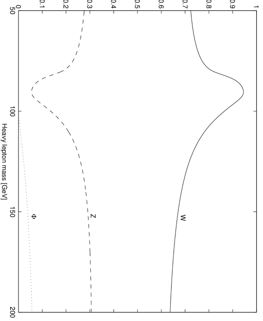
Figure 4: Branching ratios in the heavy lepton sector: $B(\ell^{H}\to\ell^{L}X)$ where $X$ is W, Z, or $\Phi$. We set $v\lambda_{\ell}=2\,m_{\tau}^{L}$ and $M_{\Phi}=100$ GeV.

The branching fractions for decays of the heavy down-type quarks display a significant flavor-dependence. Those for the $d^{H}$ and $s^{H}$ are essentially identical and resemble the branching fractions for the heavy leptons. However, charged-current decays of $b^{H}$ with a mass less than 255 GeV (the threshold for decay to an on-shell top and W) are doubly Cabbibo-suppressed, so that the $b^{H}$ branching ratios do not resemble those of the other down-type quarks. Generally speaking, a $b^{H}$ of relatively low mass decays almost exclusively by the process $b^{H}\to Zb^{L}$. For $m^{b}_{H}$ larger than 255 GeV, the decay $b^{H}\to t^{L}W$ dominates and the Z-mode branching fraction is only about half as large. If $m_{b}^{H}$ is above $M_{\Phi}+m_{b}^{L}$ but below 255 GeV, the scalar decay mode becomes significant (in agreement with reference [23]). If the scalar mass lies above 255 GeV, the scalar decay mode is much less important. In the asymptotic regime, where $m_{D}^{H}$ is much greater than $m_{t}$ or any boson’s mass, the branching ratios for decays to W, Z, and $\Phi$ approach $49\%$, $25\%$, and $26\%$, respectively.

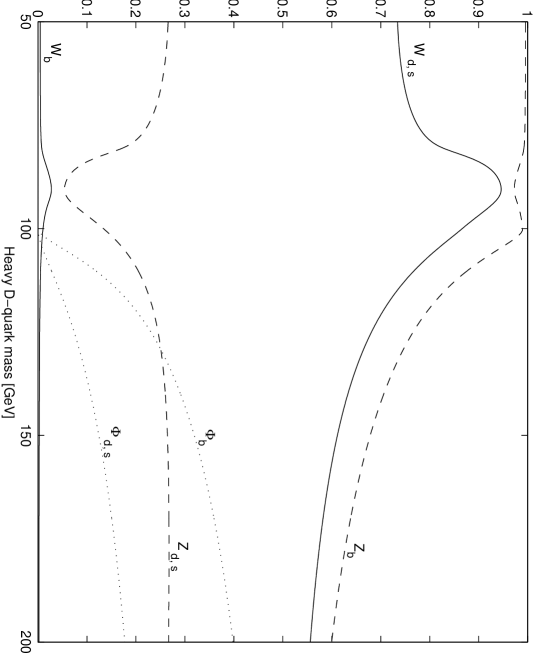
Figure 5: Branching ratios in the heavy down-quark sector: $B(D^{H}\to D^{L}X)$ where $X$ is W, Z, or $\Phi$. Subscripts d, s, and b denote the heavy quarks’ flavor. We set $v\lambda_{D}=2\,m_{b}^{L}$ and $M_{\Phi}=100$ GeV.

5.2 Heavy leptons at LEP II

The LEP II experiments have searched for evidence of new sequential leptons, working under the assumptions that the new neutral lepton $N$ is heavier than its charged partner $L$ and that $L$ decays only via charged-current mixing with a Standard Model lepton (i.e. $B(L\to\nu_{\ell}W^{*})=$ 100%). Recent limits from the OPAL experiment at $\sqrt{s}=172$ GeV [10] and from the DELPHI experiment at $\sqrt{s}=183$ GeV [11] each set a lower bound of order 80 GeV on the mass of a sequential charged lepton.

To illustrate how the LEP limits may be applied to our weak-singlet fermions, we review OPAL’s analysis. The OPAL experiment searched for pair-produced charged sequential leptons undergoing charged-current decay:

$$e^{+}e^{-}\to L^{+}L^{-}\to\nu_{\ell}\bar{\nu_{\ell}}W^{+}W^{-}$$ (5.4)

Their cuts selected final states in which at least one of the $W^{*}$ bosons decayed hadronically. Events with no isolated lepton were required to have at least 4 jets and substantial missing transverse momentum; those with one or more isolated leptons were required to have at least 3 jets, less than 100 GeV of visible energy, and substantial missing transverse momentum. The efficiencies for selecting signal events were estimated at 20-25% by Monte Carlo. With 1 candidate event in the data set and the expectation of 3 Standard Model background events, OPAL excluded, at 95% c.l., sequential leptons of mass less than 80.2 GeV, as these would have contributed least 3 signal events to the data.

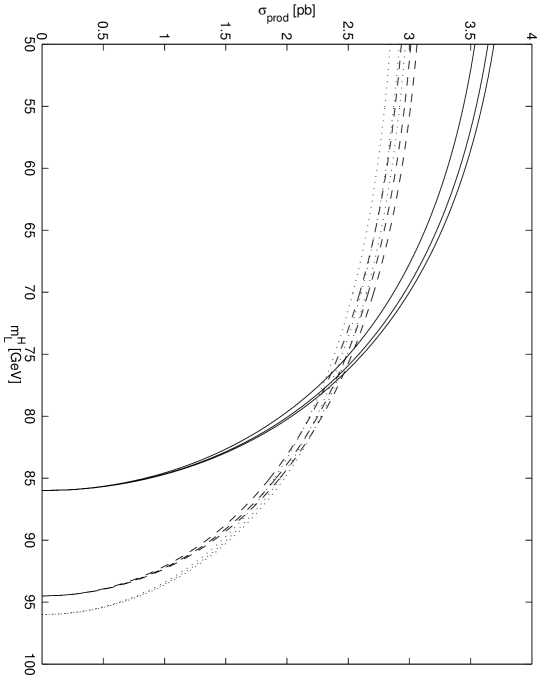
Figure 6: Production cross-section for a heavy lepton that is mostly weak-singlet as a function of lepton mass and mixing angles. Each family of curves represents one value of $\sqrt{s}$ (solid = 172 GeV, dashed = 189 GeV, dotted = 192 GeV). The separate curves within each family show the effect of changing the value of the small mixing angles (top curve: $\sin^{2}\phi_{\ell}$ = 0.1 for all leptons, middle curve: $\sin^{2}\phi_{\ell}=0$ for all leptons, bottom curve: $\sin^{2}\phi_{e}$ = 0, $\sin^{2}\phi_{\mu,\tau}$ = 0.1).

The heavy leptons in the models we are studying have different weak quantum numbers than those OPAL sought. This alters both the production rate and the decay paths of the leptons. The production rate of the $\ell^{H}$ should be larger than that for the sequential leptons. The pure QED contribution is the same, as the heavy leptons have standard electric charges; the weak-electromagnetic interference term is enhanced since the coupling to the $Z$ is roughly $\sin^{2}\theta_{W}>0$ rather than $\sin^{2}\theta_{W}-0.5<0$ as in the Standard Model. By adapting the results of reference [24] to include the couplings appropriate to our model, we have evaluated the production cross-section for heavy leptons at LEP II. Our results are shown in figure 6 as a function of heavy lepton mass for several values of $\sqrt{s}$ and lepton mixing angle.

On the other hand, the likelihood that our heavy leptons decay to final states visible to OPAL is less than it would be for heavy sequential leptons. In events where both of the produced $\ell^{H}$ decay via charged-currents, about 90% of the subsequent (standard) decays of the $W$ bosons lead to the final states OPAL sought – just as would be true for sequential leptons. But the heavy leptons in our model are not limited to charged-current decays. In events where one or both of the produced $\ell^{H}$ decay through neutral currents, the result need not be a final state visible to OPAL. If there is one W and one Z in the intermediate state, about 36% of the events should yield final states with sufficient jets, isolated leptons and missing energy to pass the OPAL cuts. At the other extreme, if both $\ell^{H}$ decay by $\Phi$ emission, there will be virtually no final states with sufficient missing energy, since $\Phi$ decays mostly to $b\bar{b}$. The other decay patterns lie in between; for intermediate $ZZ$ ($\Phi Z$, $\Phi W$) we expect 28% (19%, 30%) of the events to be visible to OPAL. The total fraction of pair-produced heavy leptons that yield appropriate final states is the sum of these various possibilities:

$$B_{decay} = 0.896\,(B_{W})^{2}+0.280\,(B_{Z})^{2}+2\,(\,0.361\,B_{W}\cdot B_{Z}$$ (5.5)

$$+ 0.190\,B_{Z}\cdot B_{\Phi}\,+\,0.306\,B_{\Phi}\cdot B_{W}\,)$$

where $B_{W}$, $B_{Z}$, and $B_{\Phi}$ are the heavy lepton branching fractions for the W, Z and scalar decay modes respectively, as calculated in section 5.1 (and shown in Figure 4).

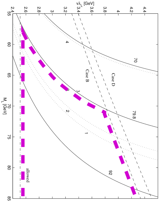
Figure 7: Lower bounds on heavy lepton mass in models with one flavor of heavy lepton (Cases B and D). The heavy dashed curve encloses the region of the plot allowed by the combination of electroweak and direct search data. The limits on $\sin{\phi_{\tau}}^{2}$ (dashed lines) and $v\lambda_{\ell}=m^{L}_{\tau}\sqrt{2}$ (dot-dash line) are as in Figure 1. Solid lines are contours of constant heavy lepton mass $m^{H}_{\tau}$; dotted curves are contours of constant numbers of OPAL signal events. The lower bound the lepton mass comes from the overlap of the limiting $N=3$ dotted line with the $m^{H}_{\tau}=79.8\ {\rm GeV}$ solid line. In calculating branching fractions, the scalar mass was set to 100 GeV.

In models (cases B and D) where there is only one species of heavy lepton ($\tau^{H}$), setting a mass limit is straightforward. We note that

$$\sigma_{production}\cdot B_{decay}=N_{events}/\epsilon\cdot{\cal L}$$ (5.6)

where, as in OPAL’s analysis, the integrated luminosity is ${\cal L}=10.3\,pb^{-1}$, the signal detection efficiency is $\epsilon\approx 20\%$, and the number of (unseen) signal events is $N_{events}\approx 3$. Thus an upper bound on the number of signal events implies an upper bound on $\sigma_{production}\cdot B_{decay}$. Inserting the branching fraction for $\ell^{H}\ell^{H}$ pairs to visible final states, $B_{decay}$, as in equation (5.5) yields an upper bound on the production cross-section. Since we have already calculated the cross-section ($\sigma_{production}(\sqrt{s}=172\ {\rm GeV})$) as a function of heavy lepton mass, we can convert the bound on $\sigma_{production}$ into a a $95\%$ c.l. lower bound on $m^{H}_{\tau}$:

$$m^{H}_{\tau}>79.8\ {\rm GeV}.$$ (5.7)

This is a great improvement over the bounds of order 40 GeV, (4.22) and (4.25), we obtained earlier from precision electroweak data in cases B and D where the tau is the only lepton to have a weak-singlet partner.

Our new lower bound on $m^{H}_{\tau}$ further constrains the allowed region of the $M_{\ell}{\,}$vs.${\,}v\lambda_{\ell}$ parameter space, as illustrated in figure 7. Contours on which the heavy tau mass takes on the values $m_{\tau}^{H}=70,\,79.8$ and $92$ GeV are shown as a reference and to indicate how a tighter mass bound would affect the size of the allowed region.

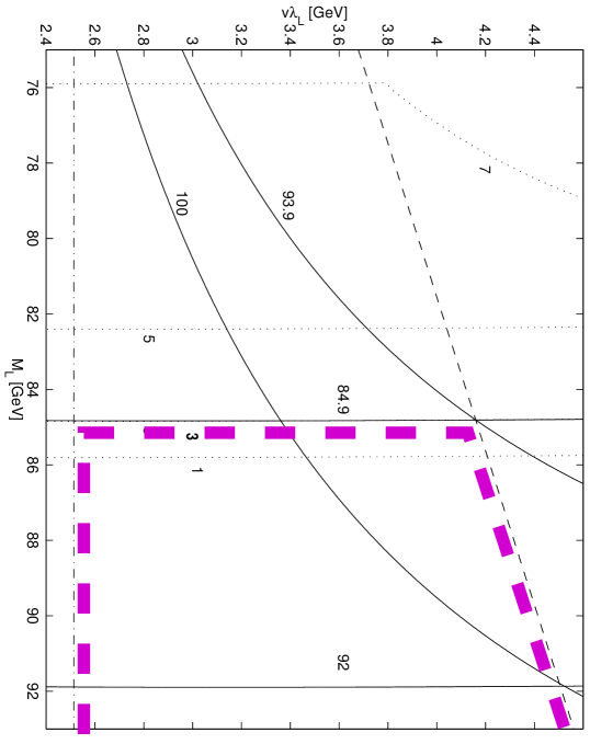
Figure 8: Lower bounds on heavy lepton mass in models with three flavors of heavy lepton (Case A). The heavy dashed curve encloses the region of the plot allowed by the combination of electroweak and direct search data. The limits on $\sin{\phi_{\tau}}^{2}$ (dashed lines) and $v\lambda_{\ell}=m^{L}_{\tau}\sqrt{2}$ (dot-dash line) are as in Figure 1. Solid lines are contours of constant heavy lepton mass - those for $m^{H}_{e,\mu}$ are vertical, those for $m^{H}_{\tau}$ are curved. Dotted lines are contours of constant number of OPAL signal events; the cusp shows where the pair-production threshold for $\tau^{H}$ is crossed. The mass limit for $e^{H},\mu^{H}$ comes from the overlap of the $N_{events}=3$ dotted line with the $m^{H}_{e,\mu}=84.9\ {\rm GeV}$ solid line; at these values of $v\lambda_{\ell}$ and $M_{\ell}$, the $\tau^{H}$ is above OPAL’s pair-production threshold. In calculating branching fractions, the scalar mass was set to 100 GeV.

In case A, where $e$, $\mu$, and $\tau$ all have singlet partners, the contributions from all three heavy leptons to the signal have to be taken into account. While the $e^{H}$ and $\mu^{H}$ have nearly identical masses and decays, the $\tau^{H}$ has slightly different properties. By adding the contributions from all three flavors of heavy lepton, drawing the contour corresponding to $N_{events}=3$ on the $M_{\ell}{\,}$vs.${\,}v\lambda_{\ell}$ parameter space, and comparing this with contours of constant $m^{H}_{\ell}$ for each species, we obtain the 95% c.l. lower bounds on all three heavy lepton masses, as shown in figure 8

$$m^{H}_{e,\mu}>84.9\ {\rm GeV}\ \$$ (5.8)

$$m^{H}_{\tau}>93.9\ {\rm GeV}\,.$$ (5.9)

Note that the bound on $m^{H}_{\tau}$ comes simply from internal consistency of the model (the values of $v\lambda_{\ell}$ and $M_{\ell}$ are flavor-universal), since it lies above OPAL’s pair-production threshold. These bounds are a significant improvement over those we obtained from precision data, i.e. (4.15) and (4.12).

While calculating the lower limits on the $m^{H}_{\ell}$ required us to assume a value for $M_{\Phi}$ (to evaluate $B_{decay}$), the result is insensitive to the precise value chosen. As noted in section 5.1, in the allowed region of the $v\lambda_{\ell}$ vs. $M_{\ell}$ plane, LEP’s lower bound on the Higgs boson’s mass applies to $\Phi$ so that min($m_{\ell}^{H}$) $\leq$ min($M_{\Phi}$). In this case, $B(\ell^{H}\to\Phi\ell^{L})$ is negligible.

Our limits are also insensitive to the precise values of the small lepton mixing angles $\sin\phi_{\ell}$. The production rate has little dependence on $\sin\phi_{\ell}$ because the $\ell^{H}\ell^{H}Z$ coupling (2.19) is dominated by the “$-Q\sin^{2}\theta$” term. What little dependence there is on $\sin\phi_{\ell}$ decreases as $2m^{H}_{\ell}$ approaches $\sqrt{s}$, and the mass limits tend to be set quite close to the production threshold. Moreover, the branching fractions for the vector boson decays of the $\ell^{H}$ have only a weak dependence on $\sin\phi_{\ell}$. Both the charged- and neutral-current decay rates are proportional to $\sin^{2}\phi_{\ell}$ (and the rate for decay via Higgs emission is negligible), so that the mixing angle dependence in the branching ratio comes only through factors of $\cos^{2}\phi_{\ell}$ which are nearly equal to 1. As a result, our lower bounds on the heavy fermion masses will stand even if improved electroweak measurements tighten constraints on the mixing angles.

Because the mass limit tracks the pair-production threshold, stronger mass limits can be set by data taken at higher center-of-mass energies. Figure 6 shows $\sigma_{production}$ as a function of the heavy lepton mass for several values of $\sqrt{s}$ and $\sin^{2}\phi_{\ell}$. As data from higher energies provides a new, more stringent upper bound on $\sigma_{production}\cdot B_{decay}$, one can read an improved lower bound on the heavy lepton mass from figure 6.

More generally, one can infer a lower mass limit on a heavy mostly-weak-singlet lepton from other models using the same data by inserting the appropriate factor of $B_{decay}$ in equation (5.6). For models in which the mixing angles between ordinary and singlet leptons are small and in which $B(\ell^{H}\to\Phi\ell^{L})$ is small, our results apply directly. This would be true, for example, of some of the heavy leptons in the flavor-universal top seesaw models [8].

Since the lower bound the LEP II data sets on the mass of the heavy leptons is close to the kinematic threshold for pair production, it seems prudent to investigate whether single production

$$e^{+}e^{-}\to\ell^{H}\ell^{L}$$ (5.10)

would give a stronger bound. Single production proceeds only through $Z$ exchange (the $\gamma f^{H}f^{L}$ coupling is zero). Moreover, equation (2.19) shows that the $Z\ell^{H}\ell^{L}$ coupling is suppressed by a factor of $\sin\phi_{\ell}$; given the existing upper bounds on the mixing angles (3.1)-(3.4), the suppression is by a factor of at least 10. As a result, only a fraction of a single-production event is predicted to have occurred (let alone have been detected) in the 10 pb^-1 of data each LEP detector has collected – too little for setting a limit.

5.3 Heavy quarks at the Tevatron

New quarks decaying via mixing to an ordinary quark plus a heavy boson would contribute to the dilepton events used by the Tevatron experiments to measure the top quark production cross-section [12][13]. We will use the results of the existing top quark analysis and see what additional physics is excluded. If evidence of new heavy fermions emerges in a future experiment, it will be necessary to do a combined analysis that includes both the top quark and the new fermions and that examines multiple decay channels.

Here, we use the dilepton events observed at Run I to set limits on direct production of new largely-weak-singlet quarks (our $q^{H}$). These new quarks are color triplets and would be produced with the same cross-section as sequential quarks of identical mass. However, their weak-singlet component would allow the new states to decay via neutral-currents as well as charged-currents. This affects the branching fraction of the produced quarks into the final states to which the experimental search is sensitive.

The DØ and CDF experiments searched for top quark events in the reaction

$$p\bar{p}\to Q\bar{Q}\to qW\bar{q}W\ \ \to\ \ q\bar{q}\ell\nu_{\ell}\ell^{\prime}\nu_{\ell^{\prime}}$$ (5.11)

by selecting the final states with dileptons, missing energy, and at least two jets. Di-electron and di-muon events in which the dilepton invariant mass was close to the Z mass were rejected in order to reduce Drell-Yan background. The top quark was assumed to have essentially 100% branching ratio to an ordinary quark (q) plus a W, as in the Standard Model. The DØ (CDF) experiment observed 5 (9) dilepton events, as compared with 1.4 $\pm$ 0.4 (2.4 $\pm$ 0.5) events expected from Standard model backgrounds and 4.1 $\pm$ 0.7 (4.4 $\pm$ 0.6) events expected from top quark production. Thus, DØ (CDF) measured the top production cross-section to be 5.5 $\pm$ 1.8 pb ($8.2^{+4.4}_{-3.4}$ pb).

In using this data to provide limits on the production of heavy quarks in our models, we consider dilepton events arising from top quark decays to be part of the background. Hence, from DØ (CDF), we have 5 (9) dilepton events as compared with a background of 5.5 $\pm$ 0.8 (6.8 $\pm$ 0.8) events. At 95% confidence level, this implies an upper limit of 5.8 (9.6) on the number of additional events that could have been present due to production and decays of new heavy quarks.

How many $q^{H}$ would be produced and seen ? The $q^{H}$ have the same QCD production cross-section as a Standard Model quark of the same mass. The $q^{H}$ can decay by the same route as the top quark (5.11). About 10% of the charged-current decays of pair-produced $q^{H}$ would yield final states to which the FNAL dilepton searches were sensitive. The neutral current decays of the $q^{H}$ reduce the charged-current branching fraction $B(q^{H}\to q^{L}W)$, but will not, themselves, contribute significantly to the dilepton sample since dileptons from $Z$ decays are specifically rejected and the $\Phi$ couplings to $e$ and $\mu$ are extremely small. Then we estimate the fraction of heavy quark pair events that would contribute to the dilepton sample as

$$B_{decay}=B_{\ell\ell}\,(B_{W})^{2}$$ (5.12)

where $B_{\ell\ell}$ is the fraction of $W$ pairs in which both bosons decay leptonically and $B_{W}\equiv B(q^{H}\to q^{L}W)$ is calculated in section 5.1 and shown in figure 5.

The number of dilepton events expected in a heavy-quark production experiment with luminosity ${\cal L}$ and detection efficiency for dilepton events $\epsilon$ is

$$N^{q^{H}}=\sigma^{q^{H}}\cdot{\cal L}\cdot\epsilon\cdot B_{decay}$$ (5.13)

Similarly in top searches the total number of events is

$$N^{t}=\sigma^{t}\cdot{\cal L}\cdot\epsilon\cdot B_{cc}\cdot B_{\ell\ell}$$ (5.14)

where $B_{cc}$ is the fraction of top quark pairs decaying via charged currents.

In comparing the number of events expected for produced top quarks with those for $q^{H}$ pairs, the values of $\epsilon$ and ${\cal{L}}$ are the same; furthermore, $B_{cc}$ of equation (5.14) is essentially 100% . Therefore we may write

$$\sigma^{q^{H}}\,(B_{W})^{2}=\sigma^{t}\ {N^{q^{H}}\over N^{t}}$$ (5.15)

Using the values which the CDF and DØ experiments have determined for the three quantities on the right-hand side (cf. previous discussion), we find

$$\sigma^{q^{H}}\,(B_{W})^{2} \leq 7.8\ {\rm pb}\ \ ({\rm DO})$$ (5.16)

$$\leq 12.0\ {\rm pb}\ \ ({\rm CDF}).$$

The dilepton sample at the Tevatron is sensitive only to the presence of the $d^{H}$ or $s^{H}$ quarks in our models. The $u^{H}$, $c^{H}$ and $t^{H}$ are, according to equations (4.8), (4.13) and (4.16), too heavy to be produced, while the $b^{H}$ decay dominantly by neutral instead of charged currents, due to Cabibbo suppression. Hence, this search tests only the models of case A, in which the light ordinary fermions have weak-singlet partners.

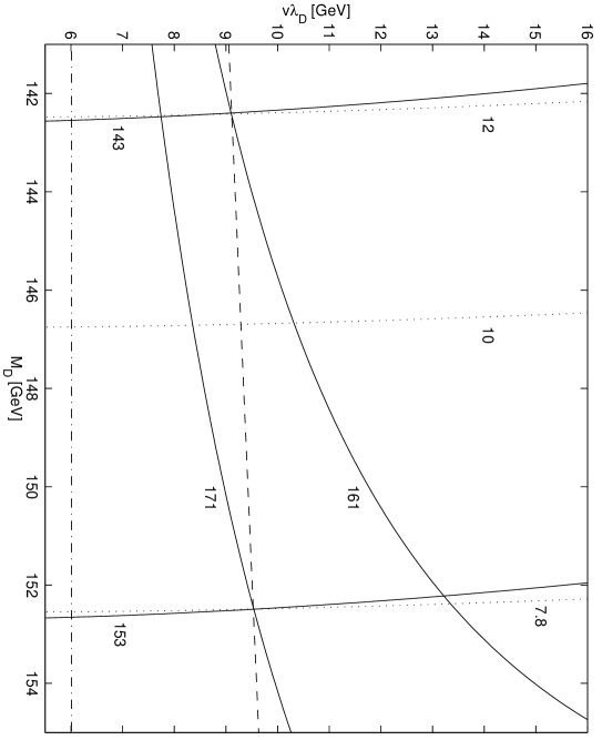
Figure 9: A graphical representation of the Tevatron limits on heavy D quark masses. The region allowed by precision electroweak tests (cf. fig 2) is bounded from above by the dashed line ($\sin{\phi_{b}}^{2}$) and from below by the dot-dashed line ($v\lambda_{D}$). Dotted lines represent curves of constant $\sigma_{prod}\cdot(B_{W})^{2}$ as in equation (5.15). Solid vertical lines are curves of constant $m^{H}_{d,s}$ ($m^{H}_{b}$); their overlap with the dotted lines defines the lower bound on the heavy fermion masses. We set $M_{\Phi}=100$ GeV in calculating branching fractions.

Since the pair-production cross-section for $q^{H}$ is the same as that for a heavy ordinary quark, we use the cross-section plots of reference [25] and our calculated branching fraction $B_{decay}$ (5.12) to translate equation (5.16) into lower bounds on heavy fermion masses. For Case A, in which both the $d^{H}$ and $s^{H}$ quarks can contribute to the dilepton sample, we find (with $M_{\Phi}=100$ GeV):

$$m^{H}_{d},m^{H}_{s} \geq 153\ {\rm GeV}\ \ ({\rm DO})$$

$$\geq 143\ {\rm GeV}\ \ ({\rm CDF})$$

$$m^{H}_{b} \geq 171\ {\rm GeV}\ \ ({\rm DO})$$ (5.17)

$$\geq 161\ {\rm GeV}\ \ ({\rm CDF}).$$

which are significantly stronger than those obtained from low-energy data in section 4 and also stronger than the published limits on a fourth-generation sequential quark [26]. Note that since the $b^{H}$ decays almost exclusively via neutral-currents due to Cabbibo suppression of the charged-current mode, the lower bound on $m^{H}_{b}$ is, once again, an indirect limit implied by internal consistency of the model. In the scenarios where only third-generation fermions have weak partners (Cases B and C), we can obtain no limit on $m_{b}^{H}$.

More generally, one can use the same data to infer an upper limit on the pair-production cross-section for heavy mostly-weak-singlet quarks from other models by inserting the appropriate factor of $B_{W}$ in equation (5.16). After taking into account the number of heavy quarks contributing, one can use the cross-section vs. mass plots of [25] to determine lower bounds for the heavy quark masses. For example, our cross-section limits (5.16) apply directly to the heavy mostly-singlet quarks in the dynamical top-seesaw models that are kinematically unable to decay to scalars and decay primarily by charged-currents. The corresponding mass limit depends on how many such quarks are in the model.

6 Oblique Corrections

The presence of new singlet fermions present in our models will shift the $S$ and $T$ parameters [27] from their Standard Model values. In this section, we evaluate these changes and explore the limits they impose on the fermion masses and couplings and the mass of the scalar, $\Phi$. This analysis of one-loop oblique corrections turns out to complement the analysis of tree-level effects on precision data performed in section 3: the oblique corrections most strongly limit the top quark mixing angle which the earlier analysis could not directly constrain.

In calculating the values of $S$ and $T$ predicted by our models, we started from the results of [29], which cite the experimental values of $S$ and $T$ relative to the reference point [$m_{t}=173.9$ GeV, $m_{H}=300$ GeV, $\alpha^{-1}(M_{Z})=128.9$]. We included the appropriately weighted variations of $m_{t}$ and $\alpha^{-1}$ and obtained the minimal combined $\chi^{2}$ field on the $S-S_{ref}$ vs $T-T_{ref}$ plane; we simultaneously obtained the corresponding $m_{t}(S,T)$ and $\alpha^{-1}(S,T)$ that minimize $\chi^{2}$ for each pair of S and T parameters. The minimal combined $\chi^{2}$ is presented in in figure 10; the solid ellipses represent joint 68.3%, 90%, and 95.4% c.l. limits on S and T with variations in $m_{t}$ and $\alpha^{-1}$ included. Next, within the Standard Model we allowed the Higgs mass to vary [28] from 40 GeV to 1 TeV in steps of 10 GeV and obtained the “best fit Higgs curve” shown in figure 10; the circled points are at 100, 200, 300, 400, and 500 GeV (smaller masses to the left). The dotted ellipses in the figure are contours of constant minimal combined $\chi^{2}$ whose intersections with the “best fit Higgs curve” define the best fit value and 68.3%, 90%, and 95.4% c.l. limits on Higgs mass. These values are respectively 80 GeV (in good agreement with [9]), 190 GeV, 310 GeV, and 400 GeV.

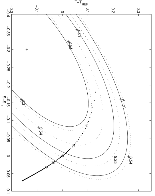
Figure 10: Comparing data on oblique corrections to theoretical predictions. Relative to the reference [$m_{t}=173.9$ GeV, $m_{H}=300$ GeV, $\alpha^{-1}(M_{Z})=128.9$], the cross shows the best experimental fit to $S$ and $T$; the solid ellipses are at the corresponding 68%, 90% and 95% confidence levels [29] for two degrees of freedom. The labels on both the solid and dotted ellipses indicate $\Delta\chi^{2}$ relative to the experimental best-fit point (cross). The heavy dotted curve shows how the predicted value of $S$ and $T$ in the Standard Model varies as the scalar mass $m_{\Phi}$ is varied by steps of 10 GeV (see text); lower masses are to the left. The value of $m_{\Phi}$ corresponding to the lowest $\chi^{2}$ (smallest dotted ellipse) is $\approx$ 80 GeV.

We then added the effects of the extra fermions on $S$ and $T$. The contribution of the singlet fermions to S was calculated numerically using the formalism described in [30]. The contribution to $T$ was found analytically [31, 32] by summing the vacuum-polarization diagrams containing the heavy and light mass-eigenstate fermions present in the model of interest. For example, in models containing weak-singlet partners for only the $t$ and $b$ quarks, we find that the contribution of the $t^{H}$, $t^{L}$, $b^{H}$ and $b^{L}$ states to the $T$ parameter is (in agreement with [7])

$$\alpha T\! - \!\alpha T_{H}={3\,G_{F}\over{8\,\pi^{2}\,\sqrt{2}}}\bigg{[}{m_{t}^{L}}^{2}\,c_{t}^{4}+{m_{b}^{L}}^{2}\,c_{b}^{4}+{m_{t}^{H}}^{2}\,s_{t}^{4}+{m_{b}^{H}}^{2}\,s_{b}^{4}$$

$$- 2\,{m_{t}^{L}}^{4}\,c_{t}^{2}\bigg{(}\,-\,{c_{t}^{2}\over{m_{t}^{L}}^{2}}\,+\,{c_{b}^{2}\over{{m_{t}^{L}}^{2}-{m_{b}^{L}}^{2}}}\,-\,{s_{t}^{2}\over{{m_{t}^{L}}^{2}-{m_{t}^{H}}^{2}}}\,+\,{s_{b}^{2}\over{{m_{t}^{L}}^{2}-{m_{b}^{H}}^{2}}}\bigg{)}\ln({m_{t}^{L}}^{2})$$

$$- 2\,{m_{b}^{L}}^{4}\,c_{b}^{2}\bigg{(}\,+\,{c_{t}^{2}\over{{m_{b}^{L}}^{2}-{m_{t}^{L}}^{2}}}\,-\,{c_{b}^{2}\over{m_{b}^{L}}^{2}}\,+\,{s_{t}^{2}\over{{m_{b}^{L}}^{2}-{m_{t}^{H}}^{2}}}\,-\,{s_{b}^{2}\over{{m_{b}^{L}}^{2}-{m_{b}^{H}}^{2}}}\bigg{)}\ln({m_{b}^{L}}^{2})$$

$$- 2\,{m_{t}^{H}}^{4}\,s_{t}^{2}\bigg{(}\,-\,{c_{t}^{2}\over{{m_{t}^{H}}^{2}-{m_{t}^{L}}^{2}}}\,+\,{c_{b}^{2}\over{{m_{t}^{H}}^{2}-{m_{b}^{L}}^{2}}}\,-\,{s_{t}^{2}\over{m_{t}^{H}}^{2}}\,+\,{s_{b}^{2}\over{{m_{t}^{H}}^{2}-{m_{b}^{H}}^{2}}}\bigg{)}\ln({m_{t}^{H}}^{2})$$

$$- 2\,{m_{b}^{H}}^{4}\,s_{b}^{2}\bigg{(}\,+\,{c_{t}^{2}\over{{m_{b}^{H}}^{2}-{m_{t}^{L}}^{2}}}\,-\,{c_{b}^{2}\over{{m_{b}^{H}}^{2}-{m_{b}^{L}}^{2}}}\,+\,{s_{t}^{2}\over{{m_{b}^{H}}^{2}-{m_{t}^{H}}^{2}}}\,-\,{s_{b}^{2}\over{m_{b}^{H}}^{2}}\bigg{)}\ln({m_{b}^{H}}^{2})\bigg{]}$$

where $T_{H}$ is the Higgs contribution, and $c_{f}$ ($s_{f}$) is an abbreviation for $\cos\phi_{f}$ ($\sin\phi_{f}$). To isolate the extra contribution caused by the presence of the weak-singlet partners for the $t$ and $b$ quarks, we must subtract off the amount which $t$ and $b$ contribute in the Standard Model [32]:

$$\alpha T\,-\,\alpha T_{H}={3\,G_{F}\over{8\,\pi^{2}\,\sqrt{2}}}\bigg{[}{m_{t}^{L}}^{2}\,+\,{m_{b}^{L}}^{2}\,-\,{2{m_{t}^{L}}^{2}{m_{b}^{L}}^{2}\over{{m_{t}^{L}}^{2}-{m_{b}^{L}}^{2}}}\ln\bigg{(}{{m_{t}^{L}}^{2}\over{m_{b}^{L}}^{2}}\bigg{)}\bigg{]}$$ (6.2)

Note that (6) correctly reduces to (6.2) in the limit where singlet and ordinary fermions do not mix ($\sin^{2}\phi_{t},\sin^{2}\phi_{b}\to 0$). From the form of equation (6), we see that experimental bounds on the magnitude of $T$ will constrain relatively heavy extra fermions to have small mixing angles.

To illustrate how oblique effects constrain non-standard fermions, we begin by including a weak-singlet partner only for the top quark; that is, we send $\sin^{2}\phi_{b}\to 0$ in equation (6). For a given scalar mass $m_{\Phi}$, we add to the Standard Model $S$ and $T$, the additional contribution caused by mixing of an ordinary and weak-singlet top quark. For the $T$ parameter, this extra contribution is the difference between expressions (6) and (6.2) with $\sin^{2}\phi_{b}=0$. By construction, for $s_{t}^{2}\rightarrow 0$ the new contributions to the S and T parameters both go to zero (i.e. $\delta S=\delta T=0$). When mixing is present ($s_{t}^{2}\neq 0$), one has $\delta S<0$ and $\delta T>0$, and the predicted values of $S$ and $T$ lie above the “best fit Higgs curve”

We deem “allowed” the values of $m_{t}^{H}$ and $\sin^{2}\phi_{t}$ for which the final values of $S$ and $T$ fall inside the dotted ellipse labeled $\Delta\chi^{2}$ = 5.25 – the 90% c.l. ellipse for the Standard Model alone. In other words, we require that the model including new physics agree with experiment at least as well as the Standard Model. This allows us to trace out a region of allowed heavy top mass and mixing for different values of $m_{\Phi}$, as illustrated in figure 11. Note that the presence of non-zero mixing of ordinary and singlet top quarks enables a heavier scalar to be consistent with the data.

As a complementary limit on $m_{t}^{H}$ and $\sin^{2}\phi_{t}$, we note that the discussion in section 4 requires

$$m^{H}_{t}\geq m^{L}_{t}\sqrt{1+1/\sin^{2}\phi_{t}}.$$ (6.3)

That is, for a given amount of mixing, the heavy top mass must lie above some minimum value. Combining these limits yields the allowed region in the mixing vs. mass space in figure 11. For example,

$${\rm For}\ \ m_{\phi}=100{\rm GeV},\ \ \ \ m_{t}^{H} \stackrel{{\scriptstyle>}}{{\sim}} 1450{\rm GeV}$$ (6.4)

$$\sin^{2}\phi_{t} \stackrel{{\scriptstyle<}}{{\sim}} .015$$

$${\rm For}\ \ m_{\phi}=350{\rm GeV},\ \ \ \ m_{t}^{H} \stackrel{{\scriptstyle>}}{{\sim}} 1040{\rm GeV}$$ (6.5)

$$\sin^{2}\phi_{t} \stackrel{{\scriptstyle<}}{{\sim}} .031$$

As illustrated in figure 11, if the scalar’s mass, $M_{\Phi}$, rises above 520 GeV, the regions of top mass and mixing allowed by oblique corrections by equation (6.3) cease to intersect; this provides an upper bound on the scalar mass.

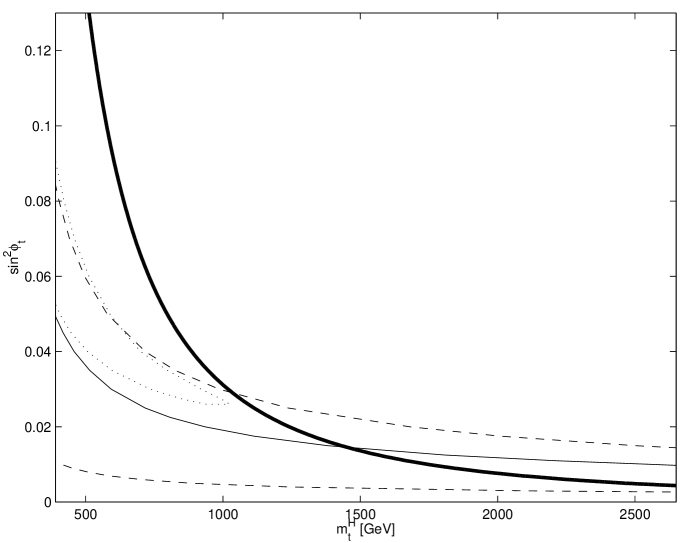
Figure 11: Lower bound on heavy top mass $m_{t}^{H}$ as a function of heavy top mixing $\sin^{2}\phi_{t}$. Based on the oblique corrections, for $m_{\Phi}$ = 100 GeV, the mass and mixing must fall below the solid curve; for $m_{\Phi}$ = 350 GeV, they must fall in the band between the dashed curves; for $m_{\Phi}$ = 520 GeV, they must lie within the dotted curve. The additional lower bound on $m_{t}^{H}$ 6.3 is represented by the heavy solid curve; the allowed region is to the right of this curve, leading to the constraints (6.4) and (6.5).

To apply oblique-correction constraints to our models, we need to include weak-singlet partners for quarks other than the top quark. Since these fermions contribute little to $S$ [27], we can illustrate the effects of including other singlet fermions by showing how they affect the $T$ parameter. First, we include the singlet partner for the $b$ quark, as in equation (6). We can interpret the result using figure 12, which shows the value of $T$ within the coupling-mass plane for the up-sector quarks. For reference, dotted nearly-vertical curves of constant heavy top mass $m_{t}^{H}$ are shown. The main contents of the figure are the three sets of curves labeled $\delta T$ = [0.3, 0.1, 0], where $\delta T$ is the contribution due to mixing between ordinary and singlet fermions. Within each set, the separate curves correspond to different values of the heavy b mass and mixing. The solid curve obtains for $m_{b}^{H}=5$ TeV and $\sin^{2}\phi_{b}=0.00090$; the dashed curve, for $m_{b}^{H}=5$ TeV and $\sin^{2}\phi_{b}=0.00040$; the doted curve, for $m_{b}^{H}=0.55$ TeV and $\sin^{2}\phi_{b}=0.00027$. Looking at the region where $m_{t}^{H}$ is of order a few TeV, we see that the influence of the b-quark is small. Including the effects of partners for the other fermions yields a generalized version of equation 6 and similar results. Thus the lower bounds on $m_{t}^{H}$ we found earlier by considering only mixing for the top quark will not be much altered by including mixing for the other quarks, as in our models A, B, and C.

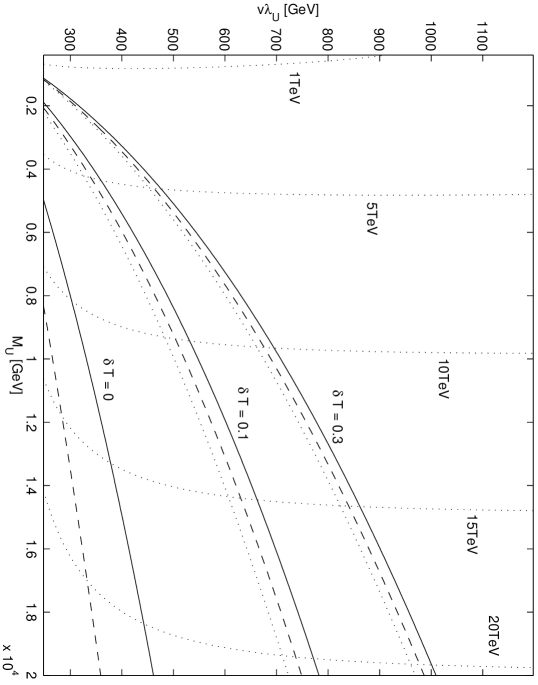
Figure 12: The effect of b-quark mixing on $T$. Contours of constant $\delta T$ are shown in the up-sector $M_{U}\,$v.s.$\,v\lambda_{U}$ parameter space. Three representative values ($\delta T$ = 0, 0.1, 0.3) are shown for several values of heavy b-quark mass and mixing. Solid curves correspond to $m^{H}_{b}=5$TeV and $\sin^{2}\phi_{b}=0.00090$ (equivalently, $M_{D}=5$TeV, $v\lambda_{D}=150$GeV). Dashed curves are $m^{H}_{b}=5$TeV and $\sin^{2}\phi_{b}=0.00040$ ($M_{D}=5$TeV, $v\lambda_{D}=100$GeV). Dotted curves are for $m^{H}_{b}=0.55$TeV and $\sin^{2}\phi_{b}=0.00027$ ($M_{D}=0.5$TeV, $v\lambda_{D}=10$GeV). The nearly-vertical dotted curves of constant $m_{t}^{H}$ are shown for reference.

7 Conclusions

Precision electroweak data constrains the mixing between the ordinary standard model fermions and new weak-singlet states to be small; our global fit to current data provides upper bounds on those mixing angles. Even when the mixing angles are small, it is possible for most of the exotic mass eigenstates which are largely weak-singlets to be light enough to be accessible to collider searches for new fermions. We have analyzed in detail a class of models in which flavor-symmetry breaking is conveyed to the ordinary fermions by soft symmetry-breaking mass terms connecting them to new weak-singlet fermions; such models have a natural GIM mechanism and a flavor structure that is stable under renormalization. By calculating the branching rates for the decays of the heavy mass-eigenstates (which are significantly influenced by their being primarily weak-singlet in nature) we have been able to adapt results from searches for new sequential fermions to further constrain our models. We find that direct searches at LEP II now imply that the heavy leptons $\ell^{H}$ must have masses in excess of 80-90 GeV; those limits are not sensitive to the precise values of the small mixing angles. Current Tevatron data indicates that heavy quark states $d^{H}$ and $s^{H}$ could be as light as about 140-150 GeV, while the mostly-weak-singlet $b^{H}$ must weigh at least 160-170 GeV. In addition, the new fermions’ contributions to the oblique corrections allow the scalar $\Phi$ to have a relatively large mass (up to about 500 GeV) while remaining consistent with the data. Oblique corrections also constrain the mixing and mass of the the heavy top state which is mostly weak-singlet; in particular, $m_{t}^{H}$ must be at least 1 TeV. Finally, we have indicated how our phenomenological results may be generalized to related models, including the dynamical top-seesaw theories.

Appendix A Appendix: Mixing effects on electroweak observables

This appendix contains the expressions for the leading-order (in mixing angles) changes to electroweak observables in the presence of fermion mixing. The expressions were derived using equations (2.16 – 2.19) and the general approach of reference [16].

$$\Delta\Gamma_{Z}/\Gamma^{SM}_{Z} = 0.603\,(\sin^{2}\phi_{e}+\sin^{2}\phi_{\mu})-0.072\,\sin^{2}\phi_{\tau}$$

$$- 0.3535\,(\sin^{2}\phi_{d}+\sin^{2}\phi_{s}+\sin^{2}\phi_{b})-0.287\,(\sin^{2}\phi_{u}+\sin^{2}\phi_{c})$$

$$\Delta\sigma_{h}/\sigma^{SM}_{h} = -1.409\,\sin^{2}\phi_{e}+0.736\,\sin^{2}\phi_{\mu}+0.072\,\sin^{2}\phi_{\tau}$$

$$- 0.1515\,(\sin^{2}\phi_{d}+\sin^{2}\phi_{s}+\sin^{2}\phi_{b})-0.124\,(\sin^{2}\phi_{u}+\sin^{2}\phi_{c})$$

$$\Delta A_{\tau}(P_{\tau})\,=\,\Delta A_{e}(P_{\tau})\,=\,\Delta A_{LR}\,=\,-0.5180\,\sin^{2}\phi_{e}+1.2870\,\sin^{2}\phi_{\mu}$$ (A.3)

$$\Delta R_{b}/R^{SM}_{b} = -0.0295\,(\sin^{2}\phi_{e}+\sin^{2}\phi_{\mu})+0.505\,(\sin^{2}\phi_{d}+\sin^{2}\phi_{s})$$ (A.4)

$$- 1.78\,\sin^{2}\phi_{b}+0.411\,(\sin^{2}\phi_{u}+\sin^{2}\phi_{c})$$

$$\Delta R_{c}/R^{SM}_{c} = 0.0605\,(\sin^{2}\phi_{e}+\sin^{2}\phi_{\mu})+0.505\,(\sin^{2}\phi_{d}+\sin^{2}\phi_{s}+\sin^{2}\phi_{b})$$ (A.5)

$$+ 0.411\,\sin^{2}\phi_{u}-1.999\,\sin^{2}\phi_{c}$$

$$\Delta A_{FB}^{b}=-0.3300\,\sin^{2}\phi_{e}+0.8500\,\sin^{2}\phi_{\mu}-0.0161\,\sin^{2}\phi_{b}$$ (A.6)

$$\Delta A_{FB}^{c}=-0.1785\,\sin^{2}\phi_{e}+0.6665\,\sin^{2}\phi_{\mu}-0.0875\,\sin^{2}\phi_{c}$$ (A.7)

$$\Delta{\cal{A}}_{b}=0.1052\,(\sin^{2}\phi_{e}+\sin^{2}\phi_{\mu})-0.1472\,\sin^{2}\phi_{b}$$ (A.8)

$$\Delta{\cal{A}}_{c}=0.5719\,(\sin^{2}\phi_{e}+\sin^{2}\phi_{\mu})-0.7997\,\sin^{2}\phi_{c}$$ (A.9)

$$\Delta Q_{W}(Cs)=72.7663\,\sin^{2}\phi_{e}-0.7239\,\sin^{2}\phi_{\mu}+211.0024\,\sin^{2}\phi_{d}-187.9988\,\sin^{2}\phi_{u}$$ (A.10)

$$\Delta Q_{W}(Tl)=111.396\,\sin^{2}\phi_{e}-4.920\,\sin^{2}\phi_{\mu}+327\,\sin^{2}\phi_{d}-285\,\sin^{2}\phi_{u}$$ (A.11)

$$\Delta R_{e}/R^{SM}_{e} = 2.275\,\sin^{2}\phi_{e}+0.130\,\sin^{2}\phi_{\mu}-0.505\,(\sin^{2}\phi_{d}+\sin^{2}\phi_{s}+\sin^{2}\phi_{b})$$ (A.12)

$$- 0.411\,(\sin^{2}\phi_{u}+\sin^{2}\phi_{c})$$

$$\Delta R_{\mu}/R^{SM}_{\mu} = 0.130\,\sin^{2}\phi_{e}+2.275\,\sin^{2}\phi_{\mu}-0.505\,(\sin^{2}\phi_{d}+\sin^{2}\phi_{s}+\sin^{2}\phi_{b})$$ (A.13)

$$- 0.411\,(\sin^{2}\phi_{u}+\sin^{2}\phi_{c})$$

$$\Delta R_{\tau}/R^{SM}_{\tau} = 0.130\,(\sin^{2}\phi_{e}+\sin^{2}\phi_{\mu})+2.145\,\sin^{2}\phi_{\tau}$$

$$- 0.505\,(\sin^{2}\phi_{d}+\sin^{2}\phi_{s}+\sin^{2}\phi_{b})-0.411\,(\sin^{2}\phi_{u}+\sin^{2}\phi_{c})$$

$$\Delta A_{FB}^{e}=-0.1230\,\sin^{2}\phi_{e}+0.3070\,\sin^{2}\phi_{\mu}$$ (A.15)

$$\Delta A_{FB}^{\mu}=0.0920\,(\sin^{2}\phi_{e}+\sin^{2}\phi_{\mu})$$ (A.16)

$$\Delta A_{FB}^{\tau}=0.0920\,\sin^{2}\phi_{e}+0.3070\,\sin^{2}\phi_{\mu}-0.2150\,\sin^{2}\phi_{\tau}$$ (A.17)

$$\Delta A_{FB}^{s}=-0.3300\,\sin^{2}\phi_{e}+0.8500\,\sin^{2}\phi_{\mu}-0.0161\,\sin^{2}\phi_{s}$$ (A.18)

$$\Delta M_{W}/M^{SM}_{W}=0.1065\,(\sin^{2}\phi_{e}+\sin^{2}\phi_{\mu})$$ (A.19)

$$\Delta g_{eV}(\nu e\rightarrow\nu e)=0.1720\,\sin^{2}\phi_{e}-0.3650\,\sin^{2}\phi_{\mu}$$ (A.20)

$$\Delta g_{eA}(\nu e\rightarrow\nu e)=0.5000\,\sin^{2}\phi_{e}-0.5060\,\sin^{2}\phi_{\mu}$$ (A.21)

$$\Delta g_{L}^{2}(\nu N\rightarrow\nu X)=0.1220\,\sin^{2}\phi_{e}+0.7260\,\sin^{2}\phi_{\mu}-0.4280\,\sin^{2}\phi_{d}-0.3445\,\sin^{2}\phi_{u}$$ (A.22)

$$\Delta g_{R}^{2}(\nu N\rightarrow\nu X)=-0.0425\,\sin^{2}\phi_{e}+0.0179\,\sin^{2}\phi_{\mu}$$ (A.23)

$$\Delta R_{\pi}/R^{SM}_{\pi}=-\sin^{2}\phi_{e}+\sin^{2}\phi_{\mu}\qquad{\rm where}\ R_{\pi}\equiv{\Gamma(\pi\to e\bar{\nu}_{e})\over{\Gamma(\pi\to\mu\bar{\nu}_{\mu})}}$$ (A.24)

$$\Delta R_{e\tau}/R^{SM}_{\tau}=\sin^{2}\phi_{\mu}-\sin^{2}\phi_{\tau}\qquad{\rm where}\ \ \ R_{e\tau}\equiv{\Gamma(\tau\to e\bar{\nu}_{e}\nu_{\tau})\over{\Gamma(\mu\to e\bar{\nu}_{e}\nu_{\mu})}}$$ (A.25)

$$\Delta R_{\mu\tau}/R^{SM}_{\mu\tau}=\sin^{2}\phi_{e}-\sin^{2}\phi_{\tau}\qquad{\rm where}\ \ \ R_{\mu\tau}\equiv{\Gamma(\tau\to\mu\bar{\nu}_{\mu}\nu_{\tau})\over{\Gamma(\mu\to e\bar{\nu}_{e}\nu_{\mu})}}$$ (A.26)

Appendix B Appendix: Details of heavy fermion decays

This appendix contains details relevant to the heavy fermion decays discussed in section 5.1.

At tree-level and neglecting final-state light fermion masses, the kinematic factors F(x,y) and G(x,y) referred to in the text have the following form:

$$F(x,y) = {1\over x^{2}}\{2\,x\,(2-x)+[3\,(x-1)+y^{2}]A(x,y)$$

$$+ [(x-1)^{2}(x+2)+3\,y^{2}(x-2)]B(x,y)\}$$

$$G(x,y) = {1\over x^{2}}\{x\,(4x-3)+[x\,(4-x)-3+y^{2}]A(x,y)$$

$$+ 2[(x-1)^{2}+y^{2}(2x-3)]B(x,y)\}$$

where A and B are given by

$$A(x,y)=\ln\bigg{[}1-{x\,(x-2)\over{(x-1)^{2}+y^{2}}}\bigg{]}$$ (B.3)

$$B(x,y)={1\over y}\,\bigg{[}\tan^{-1}\bigg{(}{1\over y}\bigg{)}-\tan^{-1}\bigg{(}{{1-x}\over y}\bigg{)}\bigg{]}$$ (B.4)

To check our general expressions for the decay rates, we evaluated their behavior in the limiting cases where the decaying heavy fermion is either much more massive or much less massive than the vector or scalar boson involved in its decay. Equations 5.1 and B for vector-boson decays yield asymptotic behavior

$$\!\Gamma(f_{i}^{H}\rightarrow f_{j}^{L}V)\,\stackrel{{\scriptstyle\scriptstyle m^{\scriptscriptstyle H}_{f_{i}}\gg M_{\scriptscriptstyle V}}}{{\longrightarrow}}\,{(c^{V}_{ij})^{2}\over{32\,\pi}}\,{{m^{H}_{f_{i}}}^{3}\over{M_{V}}^{2}}\bigg{(}1-{{M_{V}}^{2}\over{m^{H}_{f_{i}}}^{2}}\bigg{)}^{2}\,\bigg{(}1+2{{M_{V}}^{2}\over{m^{H}_{f_{i}}}^{2}}\bigg{)}$$ (B.5)

$$\Gamma(f_{i}^{H}\rightarrow f_{j}^{L}V\rightarrow f_{j}^{L}f_{k}^{L}f_{l}^{L})\,\stackrel{{\scriptstyle\scriptstyle m^{\scriptscriptstyle H}_{f_{i}}\ll M_{\scriptscriptstyle V}}}{{\longrightarrow}}$$ (B.6)

$${(c^{V}_{ij}\,c^{V}_{kl})^{2}\over{3\,\pi^{3}\,2^{9}}}{{m^{H}_{f_{i}}}^{5}\over M_{V}^{4}}\,\bigg{(}1\! + \!{3\over 5}\,{{m^{H}_{f_{i}}}^{2}\over M_{V}^{2}}\,+\,{2\over 5}\,{{m^{H}_{f_{i}}}^{4}\over M_{V}^{4}}\,+\,{2\over 7}\,{{m^{H}_{f_{i}}}^{6}\over M_{V}^{6}}\,+\cdots\bigg{)}$$

where V may be either Z or W. Equations 5.1 and B for scalar-boson decays yield

$$\Gamma(f_{i}^{H}\rightarrow f_{j}^{L}\Phi)\,\stackrel{{\scriptstyle\scriptstyle m^{\scriptscriptstyle H}_{f_{i}}\gg M_{\scriptscriptstyle\Phi}}}{{\longrightarrow}}\,{(c^{H}_{ij})^{2}\over{32\,\pi}}\,{{m^{H}_{f_{i}}}^{3}\over M_{\Phi}^{2}}\bigg{(}1-{M_{\Phi}^{2}\over{m^{H}_{f_{i}}}^{2}}\bigg{)}^{2}\\$$ (B.7)

$$\Gamma(f_{i}^{H}\rightarrow f_{j}^{L}\Phi\rightarrow f_{j}^{L}f_{k}^{L}f_{l}^{L})\,\stackrel{{\scriptstyle\scriptstyle m^{\scriptscriptstyle H}_{f_{i}}\ll M_{\scriptscriptstyle\Phi}}}{{\longrightarrow}}$$ (B.8)

$${(c^{H}_{ij}\,c^{H}_{kl})^{2}\over{3\,\pi^{3}\,2^{11}}}{{m^{H}_{f_{i}}}^{5}\over M_{\Phi}^{4}}\,\bigg{(}1 + {4\over 5}\,{{m^{H}_{f_{i}}}^{2}\over M_{\Phi}^{2}}\,+\,{3\over 5}\,{{m^{H}_{f_{i}}}^{4}\over M_{\Phi}^{4}}\,+\,{16\over 35}\,{{m^{H}_{f_{i}}}^{6}\over M_{\Phi}^{6}}\,+\cdots\bigg{)}\ .$$

Acknowledgments

The authors thank R.S. Chivukula, G. Burdman, C. Hoelbling, K. Lane, and K. Lynch for useful conversations. E.H.S. thanks the Aspen Center for Physics for hospitality during the completion of a portion of the work. E.H.S. acknowledges the support of an NSF Faculty Early Career Development (CAREER) award and an DOE Outstanding Junior Investigator award. This work was supported in part by the National Science Foundation under grant PHY-9501249, and by the Department of Energy under grant DE-FG02-91ER40676.

References

- [1] P. Langacker and D. London, Phys. Rev. D38 (1988) 886.
- [2] E. Nardi, E. Roulet, and D. Tommasini, Phys. Lett. B344 (1995) 225, hep-ph/9409310.
- [3] V. Barger, M.S. Berger, and R.J.N. Phillips, Phys. Rev. D52 (1995) 1663, hep-ph/9503204.
- [4] Particle Data Group, Euro. J. Physics C3 (1998) 1.
- [5] E.H. Simmons, Nucl. Phys. B324 (1989) 315.
- [6] B. Dobrescu and C.T. Hill, Phys. Rev. Lett. 81 (1998) 2634; R.S. Chivukula, B.A. Dobrescu, H. Georgi, and C.T. Hill, Phys.Rev. D59 (1999) 075003.
- [7] H. Collins, A. Grant, H. Georgi, HUTP-99/A043, hep-ph/9908330 (1999).
- [8] G. Burdman and N. Evans, Phys.Rev.D59 (1999) 115005.
- [9] The LEP Collaborations ALEPH, DELPHI, L3, OPAL, the LEP Electroweak Working Group and the SLD Heavy Flavour and Electroweak Groups, A Combination of Preliminary Electroweak Measurements and Constraints on the Standard Model, CERN-EP/99-15 (1999) 71pp.
- [10] OPAL Collaboration, K. Ackerstaff et al., Eur. Phys. J. C1 (1998) 45.
- [11] DELPHI Collaboration, P. Abreu et al., Eur. Phys. J. C8 (1999) 41.
- [12] The DØ Collaboration, S. Abachi et al., Phys. Rev. Lett. 79 (1997) 1203.
- [13] The CDF Collaboration, F. Abe et al., Phys. Rev. Lett. 80 (1998) 2779.
- [14] K. Chetyrkin, M. Misiak, and M. Mnz, Phys. Lett. B 400 (1997) 206; Erratum-ibid. B 425 (1998) 414; A. J. Buras, A. Kwiatkowski, and N. Pott, Phys. Lett. B 414 (1997) 157; Erratum-ibid. B 434 (1998) 459; A. J. Buras, A. Kwiatkowski, and N. Pott, Nucl. Phys. B517 (1998) 353.
- [15] CLEO Collaboration, M. S. Alam et. al., Phys. Rev. Lett. 74 (1995) 2885; ALEPH Collaboration, R.Barate et al., Phys. Lett. B 429 (1998) 169.
- [16] C.P. Burgess, S. Godfrey, H. Konig, D. London, and I. Maksymyk, Phys. Rev. D49 (1994) 6115.
- [17] LEP Electroweak Working Group Home Page, http://www.cern.ch/LEPEWWG/
- [18] W. Marciano and A. Sirlin, Phys. Rev. Lett. 71 (1993) 3639.
- [19] A. Pich and J. Silva, Phys. Rev. D52 (1995) 4006; W. Marciano and L. Sirlin, Phys. Rev. Lett. 61 (1988) 1815.
- [20] T.G. Rizzo, Phys. Rev. D22 (1980) 389; W.-Y. Keung and W.J. Marciano, Phys. Rev. D30 (1984) 248. See also, e.g., R.N. Cahn, Rep. Prog. Phys. 52 (1989) 389.
- [21] V. Barger, H. Baer, K. Hagiwara, and R.J.N. Phillips, Phys. Rev. D30 (1984) 947; I. Bigi, Y. Dokshitzer, V. Khoze, J. Khn, and P. Zervas, Phys. Lett. B 181 (1986) 157.
- [22] L3 Collaboration, CERN-EP/99-080 (1999), hep-ex/9909004.
- [23] F. del Aguila, G. L. Kane, and M. Quirs, Phys. Rev. Lett. 63 (1989) 942; M. Sher, hep-ph/9908238 v2 (1999).
- [24] A. Djouadi, Z. Phys. C 63 (1994) 317.
- [25] E. Laenen, J. Smith, and W.L. van Neerven, Phys. Lett. B 321 (1994) 254.
- [26] The DØ Collaboration, S. Abachi et al., Phys. Rev. D22 (1995) 4877.
- [27] M.E. Peskin and T.Takeuchi, Phys. Rev. D46 (1992) 381.
- [28] K. Haigwara et al., Z. Phys. C64 (1994) 559, hep-ph/9409380.
- [29] T. Takeuchi, W. Loinaz, and A.K. Grant, “Precision Tests of Electroweak Physics,” hep-ph/9904207.
- [30] M.E. Peskin and D.V. Schroeder, “An Introduction to Quantum Field Theory,” Addison-Wesley, 1995.
- [31] M. Veltman, Diagrammatica, Cambridge University Press, (1994) pp 157-162.
- [32] M. Veltman, Nucl. Phys. B123 (1977) 89.
- [33] R. S. Chivukula, N. Evans, BUHEP-99-15, hep-ph/9907414 (1999).