The static QCD potential in coordinate space with quark masses through two loops
Michael Melles
Paul Scherrer Institute, CH-5232 Villigen, PSI

Abstract

The potential between infinitely heavy quarks in a color singlet state is of fundamental importance in QCD. While the confining long distance part is inherently non-perturbative, the short-distance (Coulomb-like) regime is accessible through perturbative means. In this paper we present new results of the short distance potential in coordinate space with quark masses through two loops. The results are given in explicit form based on reconstructed solutions in momentum space in the Euclidean regime. Thus, a comparison with lattice results in the overlap region between the perturbative and non-perturbative regime is now possible with massive quarks. We also discuss the definition of the strong coupling based on the force between the static sources.

1 Introduction

The potential between two (infinitely) heavy color charges in a singlet state has been subject to theoretical investigations for more than twenty years [1, 2, 3, 4, 5]. In the non-perturbative regime it is expected to play a key role in the understanding of quark confinement and it is a major ingredient in the description of non-relativistically bound systems like quarkonia. In addition it is the basis for the definition of the lattice coupling as the potential is given by the vacuum expectation value of the Wilson loop.

In the perturbative regime it can be utilized to define a physically motivated strong coupling which automatically possesses welcome properties such as gauge invariance and decoupling of heavy flavors [6]. The potential can also be employed for a definition of the coupling from the force between the static sources [7]. The latter definition has the advantage that the $\beta$-function is unique in that no sign-change of the coupling occurs when entering the confinement regime [7]. Moreover, the heavy quark system is ideally suited to study the overlap region between the non-perturbative and perturbative treatments of QCD. This latter point is difficult to implement with massless dynamical fermions and can only be achieved in the coordinate representation.

A possibly very interesting application of the two loop mass corrections to the heavy quark potential is the effect of a massive charm loop in the $\overline{\mbox{MS}}$-bottom mass determination [8]. Using the physical $\Upsilon$-meson for this purpose, the effect of the mass shift $\delta m_{b}$ depends on $\langle\phi_{1s}|V_{F}(r,m)|\phi_{1s}\rangle$, where $\phi_{1s}$ denotes the 1s ground state wave function of the $\Upsilon$-meson and $V_{F}$ the massive fermionic corrections to the potential. The effect could be significant if the renormalization scale depends parametrically on $m_{c}$, as indicated by a BLM-analysis [8]. For a practical evaluation of these mass shifts one needs to have manageable expressions up to the required order in perturbation theory. The exact results of Ref. [9] are not suitable due to the remaining four Monte Carlo integrations. It might also be easier to perform the mass shift calculations in position space as only an integration over the relative distance $r$ would be required. In momentum space, one has an additional integral as each wave function depends on a different three-momentum ${\bf p}$.

In this paper we derive the static QCD-potential in position space with quark masses through two loops. We use the known results in momentum space [9] and derive the coordinate results through a Fourier transformation of reconstructed approximate analytical momentum space expressions. The latter step is necessary due to the complexity of the results of Ref. [9].

We begin, however, by recalling the definition of the potential through the manifestly gauge invariant vacuum expectation value of the Wilson loop. Fig. 1 displays the Wilson loop $W_{\Gamma}=\langle 0|\mbox{Tr}{\cal P}\exp\left(ig\oint_{\Gamma}dx_{\mu}A^{\mu}_{a}{\mbox{T}}^{a}\right)|0\rangle$ of spatial extension $r$ and large temporal extension $T$ with gluon exchanges indicated. The path-ordering is necessary due to the non-commutativity of the SU(3) generators $\mbox{T}^{a}$. In the perturbative analysis through two loops considered here, all spatial components of the gauge fields $A^{\mu}_{a}({\bf r},\pm T/2)$ can at most depend on a power of $\log T$ and are thus negligible here. Furthermore, $W_{\Gamma}\stackrel{{\scriptstyle T\to\infty}}{{\longrightarrow}}\exp\left(-iTE_{0}\right)$, where the ground state energy $E_{0}$ is identified with the potential $V$. Thus we arrive at the definition:

$$V(r,m)=-\lim_{T\to\infty}\frac{1}{iT}\log\langle 0|\mbox{Tr}{\cal P}\exp\left(ig\oint_{\Gamma}dx_{\mu}A^{\mu}_{a}{\mbox{T}^{a}}\right)|0\rangle$$ (1)

Writing the source term of the heavy charges, separated at the distance $r\equiv|{\bf r}-{\bf r}^{\prime}|$, as

$$J^{a}_{\mu}(x)=igv_{\mu}T^{a}\left[\delta({\bf x}-{\bf r})-\delta({\bf x}-{\bf r}^{\prime})\right]$$ (2)

and neglecting contributions connecting the spatial components, the perturbative potential is given by

$$V(r,m)=-\lim_{T\to\infty}\frac{1}{iT}\log\langle 0|\mbox{Tr}{\cal T}\exp\left(\int d^{4}xA^{a}_{\mu}(x)J^{\mu}_{a}(x)\right)|0\rangle$$ (3)

In the above equation $v_{\mu}=\delta_{\mu,0}$ due to the purely timelike nature of the sources. For the same reason the path-ordering is replaced by the time-ordering operator ${\cal T}$. Expanding Eq. 3 perturbatively we find the position space Feynman rules for the source-gluon vertex and the source propagator respectively: $igT^{a}v_{\mu}$ and $-i\theta(x_{0}-x_{0}^{\prime})\delta({\bf x}-{\bf x}^{\prime})$.

Figure 1: The Wilson-loop $\Gamma$ with large temporal extent ($T\longrightarrow\infty$) from which the position space potential is defined. Through two loops in four dimensions, gluons connecting the spatial source lines can be neglected.

The potential in momentum space is the Fourier transform of $V(r)$. It can be calculated directly in momentum space from the on-shell heavy quark anti-quark scattering amplitude (divided by i) at the physical momentum transfer q, projected onto the color singlet sector. The momentum space Feynman rule for the source propagator is identical to the one in HQET [10]: $\frac{1}{v\cdot k+i\varepsilon}$. For anti-sources, $v\longrightarrow-v$ is prescribed (or the time-ordering reversed). Fig. 2 summarizes the momentum space Feynman rules. In analogy to HQET, double lines denote the heavy source terms.

The potential can be used to define the effective charge $\alpha_{V}$ ( the so-called V-scheme) through:

$$V(Q,m)\equiv-4\pi C_{F}\frac{\alpha_{V}(Q,m)}{Q^{2}}\;\;\;,\;\;\;V(r,m)\equiv-C_{F}\frac{\alpha_{V}(r,m)}{r}$$ (4)

where $Q^{2}\equiv{\bf q}^{2}=-q^{2}$ and both expressions above are related through a Fourier-transform. The results for QCD-corrections including massless quarks have been calculated in Ref. [11], and in Ref. [12] an independent approach found a disagreement in the pure glue part of the original results. As both authors agree now on the correctness of [12], we use in momentum space:

$$\alpha_{V}(Q) = \alpha_{\overline{{\mbox{\tiny MS}}}}(\mu)\left(1+v_{1}(Q,\mu)\frac{\alpha_{\overline{{\mbox{\tiny MS}}}}(\mu)}{\pi}+v_{2}(Q,\mu)\frac{\alpha^{2}_{\overline{{\mbox{\tiny MS}}}}(\mu)}{\pi^{2}}\right)$$ (5)

with

$$v_{1}(Q,\mu) = \frac{1}{4}\left[\frac{31}{9}C_{A}-\frac{20}{9}T_{F}n_{f}+\beta_{0}\log\frac{\mu^{2}}{Q^{2}}\right]$$ (6)

$$v_{2}(Q,\mu) = \frac{1}{16}\left[\left(\frac{4343}{162}+4\pi-\frac{\pi^{2}}{4}+\frac{22}{3}\zeta_{3}\right)C_{A}^{2}-\left(\frac{1798}{81}+\frac{56}{3}\zeta_{3}\right)C_{A}T_{F}n_{f}\right.$$ (7)

$$-\left(\frac{55}{3}-16\zeta_{3}\right)C_{F}T_{F}n_{f}+\left(\frac{20}{9}T_{F}n_{f}\right)^{2}$$

$$\left.+\beta_{0}^{2}\log^{2}\frac{\mu^{2}}{Q^{2}}+\left(\beta_{1}+2\beta_{0}\left(\frac{31}{9}C_{A}-\frac{20}{9}T_{F}n_{f}\right)\right)\log\frac{\mu^{2}}{Q^{2}}\right]$$

where $\beta_{0}=\frac{11}{3}C_{A}-\frac{4}{3}T_{F}n_{f}$, $\beta_{1}=\frac{34}{3}C_{A}^{2}-\frac{20}{3}C_{A}T_{F}n_{f}-4C_{F}T_{F}n_{f}$ and $C_{A}=3$, $C_{F}=\frac{4}{3}$ and $T_{F}=\frac{1}{2}$ in QCD. The number of massless flavors is denoted by $n_{f}$. The $\beta$-function is here defined as

$$\beta(\alpha_{s}(\mu^{2}))=\frac{1}{\alpha_{s}(\mu^{2})}\frac{\partial\alpha_{s}(\mu^{2})}{\partial\log\mu^{2}}\equiv-\sum_{n=0}^{\infty}\beta_{n}\left(\frac{\alpha_{s}(\mu^{2})}{4\pi}\right)^{n+1}$$ (8)

For the case of massless quarks, the first two coefficients $\beta_{0}$ and $\beta_{1}$ are renormalization scheme invariant and the $\beta$-function is gauge invariant to all orders in minimally subtracted schemes [13].

Figure 2: The momentum space Feynman rules used in the calculation of Ref. [9]. The $i\varepsilon$-prescription is analogous to the conventional quark propagator. For anti-sources $v\longrightarrow-v$ must be used.

In coordinate space we have in the massless case [14, 15]:

$$\alpha_{V}(r) = \alpha_{\overline{{\mbox{\tiny MS}}}}(\mu)\left(1+v_{1}(r,\mu)\frac{\alpha_{\overline{{\mbox{\tiny MS}}}}(\mu)}{\pi}+v_{2}(r,\mu)\frac{\alpha^{2}_{\overline{{\mbox{\tiny MS}}}}(\mu)}{\pi^{2}}\right)$$ (9)

with

$$v_{1}(r,\mu) = \frac{1}{4}\left[\frac{31}{9}C_{A}-\frac{20}{9}T_{F}n_{f}+2\beta_{0}\log(\mu r^{\prime})\right]$$ (10)

$$v_{2}(r,\mu) = \frac{1}{16}\left[\left(\frac{4343}{162}+4\pi-\frac{\pi^{2}}{4}+\frac{22}{3}\zeta_{3}\right)C_{A}^{2}-\left(\frac{1798}{81}+\frac{56}{3}\zeta_{3}\right)C_{A}T_{F}n_{f}\right.$$ (11)

$$-\left(\frac{55}{3}-16\zeta_{3}\right)C_{F}T_{F}n_{f}+\left(\frac{20}{9}T_{F}n_{f}\right)^{2}+\beta_{0}^{2}\left(4\log^{2}(\mu r^{\prime})+\frac{\pi^{2}}{3}\right)$$

$$\left.+2\left(\beta_{1}+2\beta_{0}\left(\frac{31}{9}C_{A}-\frac{20}{9}T_{F}n_{f}\right)\right)\log(\mu r^{\prime})\right]$$

where $r^{\prime}\equiv r\exp(\gamma_{E})$.

From the renormalon point of view, possible power corrections in momentum space can at most be of the form:

$$V(Q)=-4\pi C_{F}\frac{\alpha_{\overline{{\mbox{\tiny MS}}}}(Q)}{Q^{2}}\left(1+...+const.\times\frac{\Lambda^{2}_{QCD}}{Q^{2}}+...\right)$$ (12)

which follows from Lorentz invariance (since $v.q=0$) and dimensional arguments [16]. In this connection it is interesting to note that there is a close connection between the potential and the pole mass. Both are affected by the same renormalon ambiguity and writing [16]:

$$m_{PS}(\mu_{f})\equiv m+\frac{1}{2}\int_{Q<\mu_{f}}\frac{d^{3}Q}{(2\pi)^{3}}V(Q)$$ (13)

the so-called potential subtracted mass $m_{PS}(\mu_{f})$, which depends linearly on the cutoff $\mu_{f}$, can be used as a less IR-sensitive mass parameter for threshold expansions than the pole mass $m$ [17].

In position space, however,

$$V(r)=-C_{F}\frac{\alpha_{\overline{{\mbox{\tiny MS}}}}(r)}{r}\left(1+...+const.\times\Lambda_{QCD}\;r+const^{\prime}\times\Lambda^{2}_{QCD}\;r^{2}+...\right)$$ (14)

and it is thus to be expected that the long-distance contributions to the coordinate space potential are parametrically larger than for the momentum space potential. Thus, the position space potential is likely to be more slowly convergent. This feature could be interesting when comparing the full lattice results with the perturbative solution at intermediate distances [18]. The form of the linear term in Eq. 14 is also motivating the consideration of the derivative of $V(r)$, i.e. the definition of the strong coupling from the force between the two heavy quarks [7].

Before considering the effects of massive quarks in the quantum corrections to the potential, a few general remarks are in order concerning the higher order perturbative behavior. The effective theory used for the calculation amounts to a non-local approach with $Q\sim Mv$, where $M$ denotes the heavy quark mass, i.e. where the gluons are always kept off-shell. Through power counting arguments one can see that through two loops only those gluons need to be considered. At the three loop level, however, on-shell gluon contributions of order $Q\sim Mv^{2}$ cannot be omitted and a treatment according to the standard definition would lead to an infrared divergent potential [19]. These ultra soft terms are expected to be canceled, however, by additional diagrams at that order. In particular, new diagrams connecting also the spatial components of the Wilson loop in Fig. 1 will contribute at three loops. In Ref. [20] it is indicated how the problem already shows up at the two loop level in three dimensions and in Ref. [19] an infrared save definition at higher orders is suggested. In four dimensions, however, and to the order we are working here no such problems occur and the definition 3 is infrared safe.

The paper is organized as follows. In section 2 we review the results of the mass corrections to the heavy quark potential in momentum space at the two loop order. From the physical Gell-Mann Low equation we reconstruct a simple analytical approximate expression for the one- and two-loop coefficients. These results are then used to obtain the position space potential in section 3. In section 4 we then discuss the effect of massive quarks on the force between two static sources and close with concluding remarks in section 5. Explicit results for the coupling definition through the force in coordinate space are given in the appendix, where we also discuss briefly the effect of mixed massless and massive quark loops at the two loop level.

2 Momentum space results

The Monte Carlo results of Ref. [9] can be used to obtain the two loop scale dependence of the static QCD potential in momentum space [6]. The difference to the conventional $\beta$-function in the Callan-Symanzik [21, 22] approach is that the physical quark anti-quark system is governed by the exchanged momentum and independent of the renormalization scale to each given order. Thus we follow the Gell-Mann Low approach and using a running $\overline{\mbox{MS}}$-mass $m(\mu)$ we have:

$$\alpha_{V}(Q,m(\mu)) = \alpha_{\overline{{\mbox{\tiny MS}}}}(\mu)\left(1+v_{1}(Q,m(\mu),\mu)\frac{\alpha_{\overline{{\mbox{\tiny MS}}}}(\mu)}{\pi}+v_{2}(Q,m(\mu),\mu)\frac{\alpha^{2}_{\overline{{\mbox{\tiny MS}}}}(\mu)}{\pi^{2}}\right)$$ (15)

where the massless limit of the coefficients $v_{1}$ and $v_{2}$ is given in Eqs. 6 and 7. The physical charge $\alpha_{V}(Q,m(\mu))$ cannot depend explicitly on the renormalization scale $\mu$ and the explicit $\mu$-dependence on the right-hand side of Eq. (15) cancels to the order we are working. Fig. 3 gives the Feynman diagrams for the fermionic contributions to the two-loop coefficient $v_{2}(Q,m(\mu),\mu)$. The mass-counterterm chosen for the Feynman diagram labeled $gse_{5}$ determines the mass-parameter which has to be used in the one-loop coefficient $v_{1}(Q,m(\mu),\mu)$. In Ref. [6] we considered the flavor-threshold dependence of heavy quarks and related the running mass to the pole mass which is renormalization-scale independent and gives explicit decoupling. This also provides a physical picture as well as a straightforward Abelian limit.

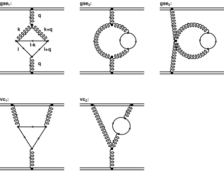
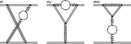
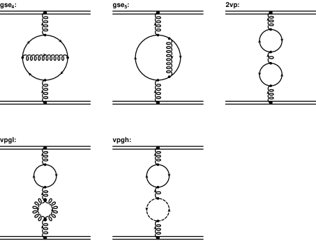
Figure 3: The two-loop massive fermionic corrections to the heavy quark potential in the Feynman-gauge (from [9]). Double lines denote the heavy quarks, single lines the “light” quarks with mass $m$. The first two rows contain diagrams with a typical non-Abelian topology. The middle line includes the infrared divergent “Abelian” Feynman diagrams. They contribute to the potential only in the non-Abelian theory due to color factors $\propto C_{F}C_{A}$. In addition, although each diagram is infrared divergent, their sum is infrared finite. The infrared finite Feynman diagrams with an Abelian topology plus the diagrams consisting of one-loop insertions with non-Abelian terms are shown in the last two rows.

The relation between the $\overline{\mbox{MS}}$ mass $m(\mu)$ and the pole mass $m$ is given by [29],

$$m(\mu)=m\left[1-C_{F}\frac{\alpha_{\overline{{\mbox{\tiny MS}}}}(\mu)}{\pi}\left(1+\frac{3}{2}\log\frac{\mu}{m}\right)\right],$$ (16)

Inserting Eq. (16) into Eq. (15) gives

$$\alpha_{V}(Q,m) = \alpha_{\overline{{\mbox{\tiny MS}}}}(\mu)\left[1+v_{1}(Q,m,\mu)\frac{\alpha_{\overline{{\mbox{\tiny MS}}}}(\mu)}{\pi}+\right.$$ (17)

$$\left.\left[v_{2}(Q,m,\mu)+\Delta_{m}(Q,m,\mu)\right]\frac{\alpha_{\overline{\mbox{\tiny MS}}}^{2}(\mu)}{\pi^{2}}\right]$$

where $\Delta_{m}(Q,m,\mu)$ denotes the contribution arising from $v_{1}$ when changing from the running mass to the pole mass: $v_{1}(Q,m(\mu),\mu)=v_{1}(Q,m,\mu)+\Delta_{m}(Q,m,\mu)\frac{\alpha_{\overline{{\mbox{\tiny MS}}}}(\mu)}{\pi}.$

The Gell-Mann Low function [23] for the $V$-scheme is defined as the total logarithmic derivative of the effective charge with respect to the physical momentum transfer scale $Q$:

$$\Psi_{V}\left(\frac{Q}{m}\right)\equiv\frac{d\alpha_{V}(Q,m)}{d\log Q}\equiv\sum^{\infty}_{i=0}-\psi_{V}^{(i)}\frac{\alpha_{V}^{i+2}(Q,m)}{\pi^{i+1}}\;,$$ (18)

where in the massless case the coefficients $\psi_{V}^{(0)}$ and $\psi_{V}^{(1)}$ are given by,

$$\psi_{V}^{(0)}\left(m=0\right) = \frac{11}{6}C_{A}-\frac{2}{3}T_{F}N_{F}=\frac{11}{2}-\frac{1}{3}N_{F}\;,$$ (19)

$$\psi_{V}^{(1)}\left(m=0\right) = \frac{17}{12}C_{A}^{2}-\frac{5}{6}C_{A}T_{F}N_{F}-\frac{1}{2}C_{F}T_{F}N_{F}=\frac{51}{4}-\frac{19}{12}N_{F}\;.$$ (20)

For the massive case all the mass effects are absorbed into a mass-dependent function $N_{F}$. In other words we write

$$\psi_{V}^{(0)}\left(\frac{Q}{m}\right) = \frac{11}{2}-\frac{1}{3}N_{F,V}^{(0)}\left(\frac{Q}{m}\right)$$ (21)

$$\psi_{V}^{(1)}\left(\frac{Q}{m}\right) = \frac{51}{4}-\frac{19}{12}N_{F,V}^{(1)}\left(\frac{Q}{m}\right)\;,$$ (22)

where the subscript $V$ indicates the scheme dependence of $N_{F,V}^{(0)}$ and $N_{F,V}^{(1)}$.

Taking the derivative of Eq. (17) with respect to $\log Q$ and re-expanding the result in $\alpha_{V}(Q,m)$ gives the following equations for the first two coefficients of $\Psi_{V}$:

$$\psi_{V}^{(0)}\left(\frac{Q}{m}\right) = -\frac{dv_{1}(Q,m,\mu)}{d\log Q}$$ (23)

$$\psi_{V}^{(1)}\left(\frac{Q}{m}\right) = -\frac{d[v_{2}(Q,m,\mu)+\Delta_{m}(Q,m,\mu)]}{d\log Q}+2v_{1}(Q,m,\mu)\frac{dv_{1}(Q,m,\mu)}{d\log Q}\;.$$ (24)

The argument $Q/m$ indicates that there is no renormalization-scale dependence in Eqs. (23) and (24). Rather, $\psi_{V}^{(0)}$ and $\psi_{V}^{(1)}$ are functions of the ratio of the physical momentum transfer $Q=\sqrt{-q^{2}}$ and the pole mass $m$ only. The expression for $\psi_{V}^{(0)}$ agrees with our result in Ref. [24]. In Eq. (24) the derivative of the $\Delta_{m}(Q,m,\mu)$-term comes from using the pole-mass instead of the MS mass whereas the remaining mass dependence in Eq. (24) is arbitrary in the sense that a different mass scheme is formally of higher order. In addition we note that the contribution $2v_{1}dv_{1}/d\log Q$ cancels the reducible contribution (labeled 2vp in Fig. 3) to $v_{2}$; it is thus sufficient to consider one quark flavor at a time for the two loop Gell-Mann Low function. In the appendix we describe how to treat the effect of massless quark loops (u,d and s) in mixed Feynman diagrams on the amplitude level as well as the case for two different mass flavor loops.

Because of the complexity of the integrals encountered in the evaluation [9] of the massive two-loop corrections to the heavy quark potential, the results were obtained numerically using the adaptive Monte Carlo integration program VEGAS [25]. Thus the derivative of the two-loop term $v_{2}$ was calculated numerically, whereas the other terms in Eqs. (23) and (24) were obtained analytically. The results are given in terms of the contribution to the effective number of flavors $N^{(0)}_{F,V}\left(\frac{Q}{m}\right)$ and $N^{(1)}_{F,V}\left(\frac{Q}{m}\right)$ in the $V$-scheme from a given quark with mass $m$ defined according to Eqs. (21) and (22) respectively. The Appelquist-Carazzone [26] theorem requires the decoupling of heavy masses at small momentum transfer for physical observables. Thus $N^{(1)}_{F,V}\left(\frac{Q}{m}\right)$ goes to zero for $Q/m\to 0$. The massless result $N_{F,V}^{(1)}\to 1$ is also be recovered for large scales.

The calculation presented in Ref. [9] required the evaluation of four-dimensional scalar integrals. The results in Ref. [6] are based on 50 iterations of the integration grid each comprising $10^{7}$ evaluations of the function which where needed to achieve adequate convergence. Even so, the Monte Carlo results still are not completely stable for small values of $Q/m$, especially in the light of the numerical differentiation required in Eq. (24). Nevertheless, accurate results can be obtained by fitting the numerical calculation to a suitable analytic function.

The one-loop contribution to the effective number of flavors $N_{F}$ follows from the standard formula for QED vacuum polarization. In Ref. [24] we used the simple representation in terms of a rational polynomial [30]:

$$N^{(0)}_{F,V}\left(\frac{Q}{m}\right)\approx\frac{1}{1+5.2\frac{m^{2}}{Q^{2}}}\equiv\frac{1}{1+a_{0}\frac{m^{2}}{Q^{2}}}$$ (25)

which displays decoupling for small scales and the correct massless limit at large scales. Similarly, the numerical results for the two-loop contribution can be fit to the form

$$N^{(1)}_{F,V}\left(\frac{Q}{m}\right)\approx\frac{a_{1}\displaystyle\frac{Q^{2}}{m^{2}}+a_{2}\displaystyle\frac{Q^{4}}{m^{4}}}{1+a_{3}\displaystyle\frac{Q^{2}}{m^{2}}+a_{2}\displaystyle\frac{Q^{4}}{m^{4}}}$$ (26)

The parameter values $a_{i}$ and the errors obtained from the fit to the numerical calculation in the $V$-scheme for QCD and QED are given in Ref. [6]. Similar decoupling forms have been used for interpolating the flavor dependence of the effective coupling in the momentum subtraction schemes (MOM) [31, 32].

In the case of QCD we obtain the following approximate form for the effective number of flavors for a given quark with pole-mass $m$:

$$N^{(1)}_{F,V}\left(\frac{Q}{m}\right)\approx\frac{\left(-0.571+0.221\displaystyle\frac{Q^{2}}{m^{2}}\right)\displaystyle\frac{Q^{2}}{m^{2}}}{1+1.326\displaystyle\frac{Q^{2}}{m^{2}}+0.221\displaystyle\frac{Q^{4}}{m^{4}}}$$ (27)

and for QED

$$N^{(1)}_{F,V}\left(\frac{Q}{m}\right)\approx\frac{\left(1.069+0.0133\displaystyle\frac{Q^{2}}{m^{2}}\right)\displaystyle\frac{Q^{2}}{m^{2}}}{1+0.402\displaystyle\frac{Q^{2}}{m^{2}}+0.0133\displaystyle\frac{Q^{4}}{m^{4}}}\;.$$ (28)

The results of our numerical calculation of $N_{F,V}^{(1)}$ in the $V$-scheme for QCD and QED are shown in Fig. 4. The decoupling of heavy quarks becomes manifest at small $Q/m$, and the massless limit is attained for large $Q/m$. The QCD form actually becomes negative at moderate values of $Q/m$, a novel feature of the anti-screening non-Abelian contributions. This property is also present in the (gauge dependent) MOM results. In contrast, in Abelian QED the two-loop contribution to the effective number of flavors becomes larger than 1 at intermediate values of $Q/m$. We also display the one-loop contribution $N^{(0)}_{F,V}\left(\frac{Q}{m}\right)$ which monotonically interpolates between the decoupling and massless limits. The solid curves displayed in Fig. 4 show that the parameterizations of Eq. (27) which we used for fitting the numerical results are quite accurate.

Figure 4: The numerical results for the gauge-invariant $N_{F,V}^{(1)}$ in QED (open circles) and QCD (triangles) with the best $\chi^{2}$ fits of Eqs. (28) and (27) superimposed respectively (from Ref. [6]). The dashed line shows the one-loop $N_{F,V}^{(0)}$ function of Eq. (25). For comparison we also show the gauge dependent two-loop result obtained in MOM schemes (dash-dot) [31, 32]. At large $\frac{Q}{m}$ the theory becomes effectively massless, and both schemes agree as expected. The figure also illustrates the decoupling of heavy quarks at small $\frac{Q}{m}$.

In Ref. [6] it was shown that the Abelian limit displayed in Fig. 4 agrees with the well known literature results [33, 34, 35] and that the full QCD result is independent of the renormalization scale. The very good agreement of the exact two loop calculation with the relatively simple fitting function for $N_{F,V}^{(1)}$ of Eq. 27 makes it possible to reconstruct an analytical approximate function for the full mass dependent two loop coefficient in the next section.

2.1 Reconstructing the momentum space potential

Starting from the general expression for the Gell-Mann Low function in Eq. 18 we can obtain $\alpha_{V}(Q,m)$ through integration over $\log Q$. Our goal is to reconstruct an analytical function for $\alpha_{V}(Q,m)$ in terms of $\alpha_{\overline{\mbox{\tiny MS}}}(\mu)$ based on the fitting parameters $a_{0}$ and $a_{1},a_{2},a_{3}$ from the approximate one- and two-loop solutions respectively. It should be clear that by analytical we mean an expression of known functions depending on $\{Q^{2},m^{2},\mu^{2},a_{0},a_{1},a_{2},a_{3}\}$ in the spacelike (Euclidean) region. It is understood that for a continuation into the timelike regime only the full function calculated in Ref. [9] can be used, not the approximate form we derive below. With this in mind we can write

$$\alpha_{V}(Q,m)-\alpha_{\overline{\mbox{\tiny MS}}}(\mu) = -\frac{\alpha^{2}_{\overline{\mbox{\tiny MS}}}(\mu)}{\pi}\left(\int\psi^{(0)}_{V}\;\;d\,\log Q+C^{(0)}\right)$$ (29)

$$-\frac{\alpha^{3}_{\overline{\mbox{\tiny MS}}}(\mu)}{\pi^{2}}\left(\int\left[\psi^{(1)}_{V}-2v_{1}\psi^{(0)}\right]d\,\log Q+C^{(1)}\right)$$

The integration constants $C^{(i)}$ can be functions of $m$ and $\mu$ and are fixed by requiring that the correct massless limit is obtained. We find for the corrections with one massive quark with pole-mass $m$:

$$v_{1}(Q,m,\mu) = \frac{31}{36}C_{A}-\frac{11}{12}C_{A}\log\frac{Q^{2}}{\mu^{2}}+\frac{T_{F}}{9}\left(-5+3\log\frac{Q^{2}+a_{0}m^{2}}{\mu^{2}}\right)$$

$$v_{2}(Q,m,\mu) = \frac{C^{2}_{A}}{16}\left(\frac{4343}{162}+4\pi^{2}-\frac{\pi^{4}}{4}+\frac{22}{3}\zeta_{3}+\frac{121}{9}\log^{2}\frac{Q^{2}}{\mu^{2}}-\frac{988}{27}\log\frac{Q^{2}}{\mu^{2}}\right)$$ (30)

$$+T_{F}\left[-\frac{C_{A}}{16}\left(\frac{1798}{81}+\frac{56}{3}\zeta_{3}\right)-\frac{C_{F}}{16}\left(\frac{55}{3}-16\zeta_{3}\right)+\frac{25}{81}T_{F}\right.$$

$$+\frac{19}{6}\left(\frac{1}{4}\log\frac{m^{4}+a_{3}m^{2}Q^{2}+a_{2}Q^{4}}{a_{2}\mu^{4}}+\frac{\frac{a_{3}}{4}-\frac{a_{1}}{2}}{\sqrt{a_{3}^{2}-4a_{2}}}\times\right.$$

$$\left.\log\frac{2a_{2}Q^{2}+(\sqrt{a_{3}^{2}-4a_{2}}+a_{3})m^{2}}{2a_{2}Q^{2}-(\sqrt{a_{3}^{2}-4a_{2}}-a_{3})m^{2}}\right)+\frac{55}{54}C_{A}\log\frac{Q^{2}}{\mu^{2}}+$$

$$\frac{31}{54}C_{A}\log\frac{Q^{2}+a_{0}m^{2}}{\mu^{2}}-\frac{10}{27}T_{F}\log\frac{Q^{2}+a_{0}m^{2}}{\mu^{2}}-\frac{11}{36}C_{A}\log^{2}\frac{Q^{2}}{\mu^{2}}$$

$$\left.-\frac{11}{18}C_{A}\log\frac{Q^{2}}{\mu^{2}}\log\frac{Q^{2}+a_{0}m^{2}}{Q\mu}+\frac{1}{9}T_{F}\log^{2}\frac{Q^{2}+a_{0}m^{2}}{\mu^{2}}\right]$$

In terms of the running mass in the $\overline{\mbox{MS}}$-scheme the solution reads:

$$v_{2}(Q,m(\mu),\mu)=v_{2}(Q,m,\mu)+\frac{1}{6}C_{F}T_{F}\frac{4+3\log\frac{\mu^{2}}{m^{2}}}{1+\frac{Q^{2}}{a_{0}m^{2}}}$$ (31)

The results are written in such a form that the limit $m\longrightarrow 0$ is obvious and can be seen to agree with Eq. 5. Eq. 31 can be directly compared to the exact calculation in Ref. [9]. The latter was obtained in the MS-scheme, so we must use

$$\mu_{\tiny{\mbox{MS}}}=\sqrt{\frac{e^{\gamma_{E}}}{4\pi}}\mu_{\overline{\tiny{\mbox{MS}}}}$$ (32)

Figure 5: The comparison between the exact results from Ref. [9] (open symbols) and the reconstructed solution in Eq. 31 (solid lines) for the bottom (triangles) and charm (circles) quarks. The absolute value of the fermionic contributions (proportional to $T_{F}$) times $\frac{1}{16\pi^{4}}$ is shown. The scale $\mu$ was chosen to coincide with the quark masses in the MS-scheme of Ref. [9]. It can clearly be seen that Eq. 31 is in good agreement with the full analytical result over all perturbative values of the momentum transfer $Q$ within the statistical Monte Carlo and fitting errors of a few percent in each case.

Fig. 5 shows the good agreement of approximate solution in Eq. 31 with the full result for different input parameters. The figure also displays the fact that the fitting parameters $a_{0},..,a_{3}$ of Ref. [6] are optimized for the flavor threshold region $Q\sim{\cal O}(m)$.

Figure 6: The momentum dependence of $\alpha_{V}(Q,m)$. We use $\mu=M_{Z}$, $\alpha_{\overline{\mbox{\tiny MS}}}(M_{Z})=0.12$ and $n_{f}=5$ throughout. The solid line is the massless result, while the two dashed lines on top of each other are massive results for the b-quark with the pole and $\overline{\mbox{MS}}$ mass.

In Fig. 6 the two loop $Q$-dependence of the physical $\alpha_{V}(Q,m)$ charge is compared with the massless calculation. In the massive result the bottom quark mass $m_{b}=4.5$GeV is used and it can be seen that the two massive results (pole and running mass) differ by several percent from the massless ($n_{f}=1$) calculation in the region $Q\sim m_{b}$. It should also be stressed that we display the full $Q$-behavior of $\alpha_{V}(Q,m)$ including constants, not just the running according to the Gell-Mann Low function.

3 Coordinate space results

In this section we will present results for the coordinate space potential based on the Fourier transform of Eq. 31. It should be emphasized that the Fourier transform of $\alpha_{V}(Q,m)$ in the strictly perturbative sense does not exist (Landau-pole) and that only the expanded coefficients can be used. This will be shown below. In general, we have the following relations:

$$V(r,m) = -C_{F}\frac{\alpha_{V}(r,m)}{r}=\int\frac{d^{3}Q}{(2\pi)^{3}}V(Q,m)\exp(i{\bf Qr})$$ (33)

$$= -4\pi C_{F}\int\frac{d^{3}Q}{(2\pi)^{3}}\frac{\alpha_{V}(Q,m)}{Q^{2}}\exp(i{\bf Qr})$$

$$= -\frac{2}{\pi}\;\frac{C_{F}}{r}\int^{\infty}_{0}\frac{dQ}{Q}\sin(Qr)\alpha_{V}(Q,m)$$

At fixed orders, there is no Landau-pole in Eq. 33 which can best be seen by inserting the expansion in Eq. 15 into Eq. 33:

$$V(r,m) = -\frac{2}{\pi}\;\frac{C_{F}\alpha_{\overline{\mbox{\tiny MS}}}(\mu)}{r}\int^{\infty}_{0}\frac{dQ}{Q}\sin(Qr)\left(1+v_{1}(Q,m,\mu)\frac{\alpha_{\overline{\mbox{\tiny MS}}}(\mu)}{\pi}\right.$$ (34)

$$+\left.v_{2}(Q,m,\mu)\left(\frac{\alpha_{\overline{\mbox{\tiny MS}}}(\mu)}{\pi}\right)^{2}\right)$$

It can easily be recognized that the first term in the series is just the Coulomb potential $V_{C}=-C_{F}\frac{\alpha_{\overline{\mbox{\tiny MS}}}(\mu)}{r}$. The loop corrections are then given by writing

$$\alpha_{V}(r,m)=\alpha_{\overline{\mbox{\tiny MS}}}(\mu)\left(1+v_{1}(r,m,\mu)\frac{\alpha_{\overline{\mbox{\tiny MS}}}(\mu)}{\pi}+v_{2}(r,m,\mu)\left(\frac{\alpha_{\overline{\mbox{\tiny MS}}}(\mu)}{\pi}\right)^{2}\right)$$ (35)

with

$$v_{1}(r,m,\mu) = \frac{C_{A}}{4}\left(\frac{31}{9}+\frac{22}{3}\left(\log(\mu\;r)+\gamma_{E}\right)\right)-\frac{5}{9}T_{F}$$ (36)

$$+\frac{T_{F}}{3}\left(\log\frac{a_{0}m^{2}}{\mu^{2}}+2\mbox{Ei}(1,\sqrt{a_{0}}\;m\;r)\right)$$

$$v_{2}(r,m,\mu) = \frac{C^{2}_{A}}{16}\left(\frac{4343}{162}+4\pi^{2}-\frac{\pi^{4}}{4}+\frac{22}{3}\zeta_{3}+\frac{121}{9}\left[4\left(\log(\mu\;r)+\gamma_{E}\right)^{2}+\frac{\pi^{2}}{3}\right]\right.$$ (37)

$$\left.+\frac{1976}{27}\left(\log(\mu\;r)+\gamma_{E}\right)\right)$$

$$+T_{F}\left[-\frac{C_{A}}{16}\left(\frac{1798}{81}+\frac{56}{3}\zeta_{3}\right)-\frac{C_{F}}{16}\left(\frac{55}{3}-16\zeta_{3}\right)+\frac{25}{81}T_{F}\right.$$

$$+\frac{19}{6}\left\{\frac{1}{4}\log\frac{(a_{3}+\sqrt{a_{3}^{2}-4a_{2}})m^{2}}{2a_{2}\mu^{2}}+\frac{1}{2}\mbox{Ei}\left(1,\sqrt{\frac{a_{3}+\sqrt{a_{3}^{2}-4a_{2}}}{2a_{2}}}\;m\;r\right)\right.$$

$$+\frac{1}{4}\log\frac{(a_{3}-\sqrt{a_{3}^{2}-4a_{2}})m^{2}}{2a_{2}\mu^{2}}+\frac{1}{2}\mbox{Ei}\left(1,\sqrt{\frac{a_{3}-\sqrt{a_{3}^{2}-4a_{2}}}{2a_{2}}}\;m\;r\right)$$

$$\left.+\frac{\frac{a_{3}}{4}-\frac{a_{1}}{2}}{\sqrt{a^{2}_{3}-4a_{2}}}\left(\log\frac{a_{3}+\sqrt{a_{3}^{2}-4a_{2}}}{a_{3}-\sqrt{a_{3}^{2}-4a_{2}}}+2\;\mbox{Ei}\left(1,\sqrt{a_{3}+\sqrt{a_{3}^{2}-4a_{2}}}\;m\;r\right)\right.\right.$$

$$\left.\left.-2\;\mbox{Ei}\left(1,\sqrt{a_{3}-\sqrt{a_{3}^{2}-4a_{2}}}\;m\;r\right)\right)\right\}-\frac{55}{27}C_{A}\left(\log(\mu\;r)+\gamma_{E}\right)$$

$$+\left(\frac{31}{54}C_{A}-\frac{10}{27}T_{F}\right)\left(\log\frac{a_{0}m^{2}}{\mu^{2}}+2\mbox{Ei}\left(1,\sqrt{a_{0}}\;m\;r\right)\right)-\frac{11}{36}C_{A}\left(\frac{\pi^{2}}{3}\right.$$

$$\left.\left.+4\left(\log(\mu\;r)+\gamma_{E}\right)^{2}\right)-\frac{11}{18}C_{A}\frac{2}{\pi}{\cal I}_{1}(r,m,\mu)+\frac{T_{F}}{9}\frac{2}{\pi}{\cal I}_{2}(r,m,\mu)\right]$$

where the integral representations are defined as follows:

$$\mbox{Ei}(1,x) \equiv \int^{\infty}_{x}\exp(-t)\frac{dt}{t}$$ (38)

$${\cal I}_{1}(r,m,\mu) \equiv \int^{\infty}_{0}\log\frac{Q^{2}+a_{0}m^{2}}{Q\mu}\log\frac{Q^{2}}{\mu^{2}}\sin(Q\;r)\frac{dQ}{Q}$$ (39)

$${\cal I}_{2}(r,m,\mu) \equiv \int^{\infty}_{0}\log^{2}\frac{Q^{2}+a_{0}m^{2}}{\mu^{2}}\sin(Q\;r)\frac{dQ}{Q}$$ (40)

Eqs. 38, 39 and 40 are readily calculable numerically, for instance with the mathematical package MATHEMATICA. Again, if one uses the $\overline{\mbox{MS}}$-running mass $m(\mu)$ instead of the above used pole mass $m$ the result must be modified in the following way:

$$v_{2}(r,m(\mu),\mu)=v_{2}(r,m,\mu)+\frac{1}{6}C_{F}T_{F}\left(4+3\log\frac{\mu^{2}}{m^{2}}\right)\left(1-\exp(-\sqrt{a_{0}}\;m\;r)\right)$$ (41)

Figure 7: The distance dependence of $\alpha_{V}(r,m)$ for the same parameters as in Fig. 6. $r$ is in GeV^-1 and $0.2\mbox{fm}\approx 1$GeV^-1.

Figure 8: The distance dependence of $\alpha_{V}(r,m)$ for different choices of the renormalization scale $\mu$. The solid line corresponds to $\mu=M_{Z}$ as in Fig. 7. The dash-dotted line to $\mu=\frac{1}{r}$ and the dashed line to the “natural choice” $\mu=\frac{1}{re^{\gamma_{E}}}$. The source separation $r$ is in GeV^-1.

The effect of the two loop mass effects in position space are depicted in Fig. 7 for the bottom quark with $m_{b}=4.5$GeV. The pole- and $\overline{\mbox{MS}}$-mass corrections are almost identical on the scale (dashed lines) and the effect grows with larger distances. Since in the renormalization group (RG) logarithms always enter as $\log(\mu r)+\gamma_{E}$, the “natural” choice is given by $\mu=\frac{1}{re^{\gamma_{E}}}$. In Ref. [27] it was shown that this scale almost identically reproduces the BLM-results [28] in the massless case, thus consistently reabsorbing the large RG-group effects. As in this case we also have to evaluate the two-loop running of the $\overline{\mbox{MS}}$-coupling using:

$$\alpha_{\overline{\mbox{\tiny MS}}}(\mu)=\frac{4\pi}{\beta_{0}\log\frac{\mu^{2}}{\Lambda^{2}_{QCD}}}\left(1-\frac{\beta_{1}}{\beta_{0}^{2}}\frac{\log\left(\log\frac{\mu^{2}}{\Lambda^{2}_{QCD}}\right)}{\log\frac{\mu^{2}}{\Lambda^{2}_{QCD}}}\right)$$ (42)

where we normalize the QCD-scale parameter $\Lambda_{QCD}$ such that $\alpha_{\overline{\mbox{\tiny MS}}}(M_{Z})=0.12$ which corresponds to $\Lambda_{QCD}=0.25$GeV and we keep $n_{f}=5$ fixed. Fig. 8 displays the effect of the various scale choices on $\alpha_{V}(r,m)$. Although the physical coupling $\alpha_{V}(r,m)$ has no renormalization scale dependence to the order we are working, the difference seen in Fig. 8 is due to uncanceled higher order terms and, in general, increases at larger distances. Substantial deviations can be seen for $\alpha_{V}(r,m)>0.2$.

Figure 9: The distance dependence of $V(r,m)$ with the same choices of the renormalization scale $\mu$ as in Fig. 8. The potential is given in units of GeV, $r$ in GeV^-1.

The potential is shown in Fig. 9 and one has to use the standard conversion factor $1\mbox{fm}^{-1}\approx 0.2$GeV in order to convert the distance to fm. Again, the scale dependence is due to higher order contributions.

Figure 10: The dependence of $\alpha_{V}(r,m)$ on the $\overline{\mbox{MS}}$ mass parameter $m(\mu)$. The figure keeps $r=0.1$ fm fixed. The diagram is displayed for the “natural choice” of the renormalization scale $\mu=\frac{1}{re^{\gamma_{E}}}$.

The mass dependence of $\alpha_{V}(r,m)$ is displayed in Fig. 10. We keep $r$ fixed at $0.1$ fm and vary the $\overline{\mbox{MS}}$-mass parameter between $0$ and $5$GeV. While perturbation theory might not be applicable for distances larger than $0.1$fm, the effect is significant and can amount to a few percent for $\overline{\mbox{MS}}$-masses up to $1$GeV for the physical charge $\alpha_{V}(r,m)$ compared to the massless result. For the bottom quark mass the effect is of order 10 % at $r=0.1$fm.

4 The force between two static sources

In this section we discuss the concept of defining the strong coupling from the force between two static color-singlet sources [7]. In coordinate space the force is simply given by:

$$F(r,m)=-\frac{\partial V(r,m)}{\partial r}\equiv-C_{F}\frac{\alpha_{F}(r,m)}{r^{2}}$$ (43)

For large distances there is no required sign change for $\alpha_{F}(r,m)$ and its accompanying $\beta$-function is unique. For the massless coupling we can simply write:

$$\alpha_{F}(r)=\alpha_{V}(r)\left(1-2\beta_{V}(\alpha_{V}(r))\right)$$ (44)

where $\beta_{V}$ denotes the massless $\beta$-function in the V-scheme. From Eq. 44 it follows directly that the massless relation between the $\alpha_{F}$-charge and the $\overline{\mbox{MS}}$-coupling to two loops is given by

$$\alpha_{F}(r)=\alpha_{\overline{\mbox{\tiny MS}}}(r^{\prime})\left(1+f_{1}\frac{\alpha_{\overline{\mbox{\tiny MS}}}(r^{\prime})}{\pi}+f_{2}\left(\frac{\alpha_{\overline{\mbox{\tiny MS}}}(r^{\prime})}{\pi}\right)^{2}\right)$$ (45)

where $r^{\prime}=r\exp(\gamma_{E})$ and the constants are given by

$$f_{1} = -\frac{35}{36}C_{A}+\frac{1}{9}T_{F}n_{f}$$ (46)

$$f_{2} = \frac{1}{16}\left[\left(-\frac{7513}{162}+\frac{229}{27}\pi^{2}-\frac{1}{4}\pi^{4}+\frac{22}{3}\zeta_{3}\right)C_{A}^{2}+\left(\frac{3410}{81}-\frac{88}{27}\pi^{2}-\frac{56}{3}\zeta_{3}\right)C_{A}T_{F}n_{f}\right.$$ (47)

$$\left.-\left(\frac{31}{3}-16\zeta_{3}\right)C_{F}T_{F}n_{f}-\left(\frac{560}{81}-\frac{16}{27}\pi^{2}\right)\left(T_{F}n_{f}\right)^{2}\right]$$

In general, the relation for the massive case is given by

$$\alpha_{F}(r,m) = -r^{2}\frac{\partial(\alpha_{V}(r,m)/r)}{\partial r}$$ (48)

$$= \alpha_{\overline{\mbox{\tiny MS}}}(\mu)\left(1+f_{1}(r,m,\mu)\frac{\alpha_{\overline{\mbox{\tiny MS}}}(\mu)}{\pi}+f_{2}(r,m,\mu)\left(\frac{\alpha_{\overline{\mbox{\tiny MS}}}(\mu)}{\pi}\right)^{2}\right)$$

at the two loop level. Explicit expressions for $f_{1}(r,m,\mu)$ and $f_{2}(r,m,\mu)$ are given in the appendix.

Figure 11: The position dependence of $\alpha_{F}(r,m)$ and the force $F$ for different choices of the renormalization scale $\mu$. The scale choice corresponding to the respective lines is the same as in Fig. 8. The force in the lower plot is in GeV², $r$ in GeV^-1.

The distance dependence of the perturbative coupling definition of $\alpha_{F}(r,m)$ is presented in Fig. 11 for the natural scale choice (dashed) and fixed $\mu=M_{Z}$ (solid). The former leads to a lower value of $\alpha_{F}(r,m)$ at larger distances. Overall, it can be seen that the coupling defined from the force is much smaller at a given source-separation $r$ than $\alpha_{V}(r,m)$ (and even smaller than $\alpha_{\overline{\mbox{\tiny MS}}}(\mu=\frac{1}{re^{\gamma_{E}}})$). Even at $r=0.2$ fm ($\equiv 1$GeV^-1) still seems to be acceptable from a perturbative point of view. This could make a comparison with lattice results very interesting. Overall, the renormalization scale dependence is also strong for $\alpha_{F}(r,m)$. The lower graph displays the force itself in units of [GeV²].

Figure 12: The dependence of $\alpha_{F}(r,m)$ on the $\overline{\mbox{MS}}$ mass parameter $\overline{m}$. The figure on the top keeps $r=0.1$ fm fixed while the one on the bottom has $r=0.2$ fm. Both diagrams are displayed to the “natural choice” of the renormalization scale $\mu=\frac{1}{re^{\gamma_{E}}}$. The effect of mass terms is clearly visible.

The mass dependence of $\alpha_{F}(r,m)$ is given in Fig. 12 analogously to Fig. 10 by varying the $\overline{\mbox{MS}}$-mass parameter between $0$ and $5$GeV and for two fixed values of $r$. The dependence on the mass terms is not as large for small $\overline{\mbox{MS}}$ in comparison to $\alpha_{V}(r,m)$, however, can still be a few percent. It can also be seen that the effect for the $\overline{\mbox{MS}}$ bottom quark mass is roughly 7% compared to the massless result at $r=0.1$fm, while it is about 10% at $r=0.2$fm.

5 Conclusions

We have calculated the coordinate space static QCD-potential through two loops with quark masses. The result is obtained by reconstructing the exact momentum space Monte Carlo results from Ref. [9] by analytically fitting the Gell-Mann Low function. The reconstructed results are in good (few percent) agreement with the fermionic results of the exact calculation. Based on these solutions we have obtained the Fourier transform in coordinate space and the force between the heavy quarks. The $\alpha_{V}(r,m)$ coupling itself grows quicker than $\alpha_{\overline{\mbox{\tiny MS}}}(\mu)$, which is mainly due to its larger value at $Q=M_{Z}$. The mass-dependence is strongest for small $\overline{\mbox{MS}}$ masses up to 1GeV at large distances (0.1fm), where the perturbative regime breaks down. At these distances the effect of keeping a massive charm or bottom quark can be a significant effect, although perturbation theory might not be trustworthy anymore at distances of order 0.1 fm. An important indicator of this fact is the strong renormalization scale dependence from uncanceled higher order terms which can lead to substantially different results.

For the corresponding definition of $\alpha_{F}(r,m)$ we find also a strong dependence on the mass terms. The effect is not as large for small $\overline{\mbox{MS}}$ masses, however can still be a few percent. At 0.2fm the effect is of order 10% for the bottom quark mass. The renormalization scale dependence from uncanceled higher order terms is also large for $\alpha_{F}(r,m)$. The overall smallness of this coupling parameter, however, indicates that it could serve as a suitable quantity to compare the perturbative and non-perturbative approaches even above scales of ${\cal O}(0.1$ fm).

In terms of practical applications, the relatively simple form of Eqs. 30 and 35 makes it possible to investigate the uncertainty of a massive charm contribution in the determination of the bottom quark mass [36].

Appendix

Explicit two loop results with quark masses for $\alpha_{F}(r,m)$

In this appendix we give the explicit expressions for the two loop results for the strong coupling parameter defined from the force between two static color singlet sources. The general definition is given in Eq. 48 and is given by:

$$f_{1}(r,m,\mu)=C_{A}\left(-\frac{35}{36}+\frac{11}{6}(\log(\mu\;r)+\gamma_{E})\right)+T_{F}\left[-\frac{5}{9}+\frac{2}{3}\exp\left(-\sqrt{a_{0}}\;m\;r\right)\right.$$

$$+\left.\frac{1}{3}\left(\log\frac{a_{0}m^{2}}{\mu^{2}}+2\;\mbox{Ei}\left(1,\sqrt{a_{0}}\;m\;r\right)\right)\right]$$ (49)

$$f_{2}(r,m,\mu)=\frac{C_{A}^{2}}{16}\left(-\frac{7513}{162}+\frac{229}{27}\pi^{2}-\frac{\pi^{4}}{4}+\frac{22}{3}\zeta_{3}-\frac{928}{27}\left(\log(\mu\;r)+\gamma_{E}\right)\right.$$

$$\left.+\frac{484}{9}\left(\log(\mu\;r)+\gamma_{E}\right)^{2}\right)$$

$$-T_{F}\left[\frac{19}{6}\left\{-\frac{1}{2}\left(\exp\left(-\sqrt{\frac{a_{3}+\sqrt{a_{3}^{2}-4a_{2}}}{2a_{2}}}\;m\;r\right)+\exp\left(-\sqrt{\frac{a_{3}-\sqrt{a_{3}^{2}-4a_{2}}}{2a_{2}}}\;m\;r\right)\right)\right.\right.$$

$$+\left.\frac{\frac{a_{3}}{2}-a_{1}}{\sqrt{a_{3}^{2}-4a_{2}}}\left(\exp\left(-\sqrt{a_{3}-\sqrt{a_{3}^{2}-4a_{2}}}\;m\;r\right)-\exp\left(-\sqrt{a_{3}+\sqrt{a_{3}^{2}-4a_{2}}}\;m\;r\right)\right)\right\}$$

$$-\frac{55}{27}C_{A}-\left(\frac{31}{27}C_{A}-\frac{20}{27}T_{F}\right)\exp\left(-\sqrt{a_{0}}\;m\;r\right)-\frac{22}{9}C_{A}\left(\log(\mu\;r)+\gamma_{E}\right)-\frac{11}{9}\frac{C_{A}}{\pi}\;r\;{\cal I}_{3}$$

$$+\frac{2}{9}\frac{T_{F}}{\pi}\;r\;{\cal I}_{4}-\left\{-\frac{C_{A}}{16}\left(\frac{1798}{81}+\frac{56}{3}\zeta_{3}\right)-\frac{C_{F}}{16}\left(\frac{55}{3}-16\zeta_{3}\right)+\frac{25}{81}T_{F}\right.$$

$$+\frac{19}{6}\left\{\frac{1}{4}\left(\log\frac{(a_{3}+\sqrt{a_{3}^{2}-4a_{2}})m^{2}}{2a_{2}\mu^{2}}+2\mbox{Ei}\left(1,\sqrt{\frac{a_{3}+\sqrt{a_{3}^{2}-4a_{2}}}{2a_{2}}}\;m\;r\right)\right.\right.$$

$$+\left.\log\frac{(a_{3}-\sqrt{a_{3}^{2}-4a_{2}})m^{2}}{2a_{2}\mu^{2}}+2\mbox{Ei}\left(1,\sqrt{\frac{a_{3}-\sqrt{a_{3}^{2}-4a_{2}}}{2a_{2}}}\;m\;r\right)\right)$$

$$+\frac{\frac{a_{3}}{4}-\frac{a_{1}}{2}}{\sqrt{a_{3}^{2}-4a_{2}}}\left(\log\frac{a_{3}+\sqrt{a_{3}^{2}-4a_{2}}}{a_{3}-\sqrt{a_{3}^{2}-4a_{2}}}+2\mbox{Ei}\left(1,\sqrt{a_{3}+\sqrt{a_{3}^{2}-4a_{2}}}\;m\;r\right)\right.$$

$$\left.\left.-2\mbox{Ei}\left(1,\sqrt{a_{3}+\sqrt{a_{3}^{2}-4a_{2}}}\;m\;r\right)\right)\right\}-\frac{55}{27}C_{A}(\log(\mu\;r)+\gamma_{E})$$

$$+\left(\frac{31}{54}C_{A}-\frac{10}{27}T_{F}\right)\left(\log\frac{a_{0}m^{2}}{\mu^{2}}+2\mbox{Ei}\left(1,\sqrt{a_{0}}\;m\;r\right)\right)$$

$$-\frac{11}{36}C_{A}\left(4\left(\log(\mu r)+\gamma_{E}\right)^{2}+\frac{\pi^{2}}{3}\right)\left.\left.-\frac{11}{9}\frac{C_{A}}{\pi}{\cal I}_{1}+\frac{2}{9}\frac{T_{F}}{\pi}{\cal I}_{2}\right\}\right]$$ (50)

where

$${\cal I}_{3}(r,m,\mu) \equiv \int^{\infty}_{0}\log\frac{Q^{2}+a_{0}m^{2}}{Q\mu}\log\frac{Q^{2}}{\mu^{2}}\cos(Q\;r)dQ$$ (51)

$${\cal I}_{4}(r,m,\mu) \equiv \int^{\infty}_{0}\log^{2}\frac{Q^{2}+a_{0}m^{2}}{\mu^{2}}\cos(Q\;r)dQ$$ (52)

For the running $\overline{\mbox{MS}}$-mass one needs to add the following contributions:

$$f_{2}(r,m(\mu),\mu) = f_{2}(r,m,\mu)-\frac{1}{6}C_{F}T_{F}\left(4+3\log\frac{\mu^{2}}{m^{2}}\right)\left(\sqrt{a_{0}}m\;r\;\exp\left(-\sqrt{a_{0}}\;m\;r\right)\right.$$ (53)

$$\left.-\left(1-\exp\left(-\sqrt{a_{0}}\;m\;r\right)\right)\right)$$

Mixed massive and massless fermionic contributions at the two loop level

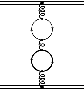
Figure 13: The Feynman diagram which can contain both massless and massive (thick line) quark loops or two flavors of different non-zero mass at the two loop level.

In this part of the appendix we briefly comment on the type of contribution depicted in Fig. 13. This diagram can contain the same flavor in both loops as well as different ones. In the former case, the contribution is already contained in the discussion above. In section 2.1 we demonstrated that for the Gell-Mann Low function only one flavor needs to be considered. On the level of the potential, however, we have also the latter case represented in Fig. 13.

In a practical situation, we can often set the masses of the three lightest quarks, u,d and s to zero. In this case the Feynman graph 13 contributes with a multiplicity factor two and we find the resulting expression:

$$2\times\mbox{Fig.13}_{0,m}\!\!\!\! = \!\!\!\!-2\frac{4\pi C_{F}}{Q^{2}}\left(\frac{31}{36}C_{A}-\frac{5}{9}T_{F}n_{f}+\frac{1}{4}\beta_{0}\log\frac{\mu^{2}}{Q^{2}}\right)\times$$ (54)

$$\!\!\!\!\left(\frac{31}{36}C_{A}-\frac{5}{9}T_{F}+\frac{11}{12}C_{A}\log\frac{\mu^{2}}{Q^{2}}-\frac{1}{3}T_{F}\log\frac{\mu^{2}}{Q^{2}+a_{0}m^{2}}\right)\frac{\alpha_{\overline{\tiny{\mbox{MS}}}}^{3}(\mu)}{\pi^{2}}$$

In the case of two non-zero and different quark loops we find analogously:

$$2\times\mbox{Fig.13}_{m,m^{\prime}}\!\!\!\! = \!\!\!\!-2\frac{4\pi C_{F}}{Q^{2}}\left(\frac{31}{36}C_{A}-\frac{5}{9}T_{F}+\frac{11}{12}C_{A}\log\frac{\mu^{2}}{Q^{2}}-\frac{1}{3}T_{F}\log\frac{\mu^{2}}{Q^{2}+a_{0}m^{2}}\right)\times$$ (55)

$$\!\!\!\!\left(\frac{31}{36}C_{A}-\frac{5}{9}T_{F}+\frac{11}{12}C_{A}\log\frac{\mu^{2}}{Q^{2}}-\frac{1}{3}T_{F}\log\frac{\mu^{2}}{Q^{2}+a_{0}{m^{\prime}}^{2}}\right)\frac{\alpha_{\overline{\tiny{\mbox{MS}}}}^{3}(\mu)}{\pi^{2}}$$

In the above expressions we used again the approximate one loop solution for the vacuum approximation. If desired, it can of course be substituted with the exact function containing more complicated expressions [24]. We also already divided by a factor $i$ to obtain the contribution to the potential.

References

• [1] L. Susskind, Coarse Grained QCD, edited by R. Balien and C.H. Llewellyn Smith (North-Holland, Amsterdam, 1977).
• [2] W. Fischler, Nucl. Phys. B129, 157 (1977).
• [3] T. Appelquist, M. Dine, I.J. Muzinich, Phys. Lett. B69, 231 (1977); Phys. Rev. D17, 2074 (1978).
• [4] F.L. Feinberg, Phys. Rev. Lett 39, 316 (1977); Phys. Rev. D17, 2659 (1978); S. Davis, F.L. Feinberg, Phys. Lett. B78, 90 (1978).
• [5] A. Billoire, Phys. Lett. B92, 343 (1980).
• [6] S.J. Brodsky, M. Melles, J. Rathsman, Phys.Rev. D60:096006, 1999.
• [7] G. Grunberg, Phys.Rev. D40, 680, 1989.
• [8] A.H. Hoang, A.V. Manohar, CERN-TH-99-357, Nov 1999. 7pp; hep-ph/9911461.
• [9] M. Melles, Phys.Rev.D58:114004,1998.
• [10] M. Neubert, Phys.Rept.245:259-396,1994.
• [11] M. Peter, Phys. Rev. Lett. 78, 602 (1997); Nucl. Phys. B 501, 471 (1997).
• [12] Y. Schröder, Phys.Lett. B447:321-326,1999 .
• [13] J. Collins, Renormalisation, Cambridge University Press, Cambridge, England, 1984.
• [14] Y. Schröder, contribution to QCD’99, Montepellier, France; hep-ph/9909520.
• [15] M. Jezabek, M. Peter, Y. Sumino, Phys.Lett. B428:352-358,1998.
• [16] M. Beneke, Phys.Rept. 317:1-142,1999.
• [17] M. Beneke, Phys.Lett. B434:115-125,1998.
• [18] G.S. Bali, Phys.Lett. B460:170-175,1999.
• [19] N. Brambilla, A. Pineda, J. Soto, A. Vairo, Phys.Rev. D60:091502,1999; CERN-TH-99-199, Jul 1999. 38pp.; hep-ph/9907240.
• [20] Y. Schröder, DESY-THESIS-1999-021, Jun 1999. 84pp.
• [21] C.G. Callan, Phys.Rev. D2:1541, 1970.
• [22] K. Symanzik, Comm.Math.Phys. 18:227, 1970.
• [23] M. Gell-Mann, F.E. Low, Phys.Rev. 95:1300, 1954.
• [24] S.J. Brodsky, M.S. Gill, M. Melles, J. Rathsman, Phys.Rev. D58:116006, 1998.
• [25] P. Lepage, VEGAS, an adaptive Monte Carlo integrator; freely available, Cornell University, 1995.
• [26] T. Appelquist, J. Carazzone, Phys.Rev. D11:2856, 1975.
• [27] M. Peter, Doctoral Thesis, Karlsruhe University, 1997.
• [28] S.J. Brodsky, G.P. Lepage, P.B. Mackenzie, Phys. Rev. D28:228, 1983.
• [29] R. Tarrach, Nucl.Phys. B183:384, 1981.
• [30] A.De Rujula, H. Georgi, Phys.Rev. D13:1296, 1976.
• [31] T. Yoshino, K. Hagiwara, Z.Phys. C24:185, 1984.
• [32] F. Jegerlehner, O.V. Tarasov, Nucl.Phys. B549:481-498,1999.
• [33] G. Källen, A. Sabry, Dan.Mat.Fys.Medd. 29, No.17, 1955.
• [34] R. Barbieri, E. Remiddi, Nuovo Cimento A13:99, 1973.
• [35] B.A. Kniehl, Nucl.Phys. B347:65, 1990.
• [36] A.H. Hoang, M. Melles, in preparation.