FISIST/1-2000/CFIF

hep-ph/0001264

Neutrino physics

E. Kh. Akhmedov
Centro de Física das Interacções Fundamentais (CFIF)

Departamento de Física, Instituto Superior Técnico
Av. Rovisco Pais, P-1049-001, Lisboa, Portugal

In the present lectures the following topics are considered: general properties of neutrinos, neutrino mass phenomenology (Dirac and Majorana masses), neutrino masses in the simplest extensions of the standard model (including the seesaw mechanism), neutrino oscillations in vacuum, neutrino oscillations in matter (the MSW effect) in 2- and 3-flavour schemes, implications of CP, T and CPT symmetries for neutrino oscillations, double beta decay, solar neutrino oscillations and the solar neutrino problem, and atmospheric neutrinos. We also give a short overview of the results of the accelerator and reactor neutrino experiments and of future projects. Finally, we discuss how the available experimental data on neutrino masses and lepton mixing can be summarized in the phenomenologically allowed forms of the neutrino mass matrix.

1 Introduction

In June of 1998 a very important event in neutrino physics occured – the Super-Kamiokande collaboration reported a strong evidence for neutrino oscillations in their atmospheric neutrino data [1]. This was not a thunderstorm in a clear sky: the evidence for oscillating neutrinos has been mounting during the last two decades in the solar neutrino experiments [2], and previous data on atmospheric neutrinos also gave indications in favour of neutrino oscillations [3]. In addition, the LSND Collaboration has reported an evidence for $\bar{\nu}_{\mu}\leftrightarrow\bar{\nu}_{e}$ and $\nu_{\mu}\leftrightarrow\nu_{e}$ oscillations in their accelerator neutrino experiment [4]. However, it was the Super-Kamiokande experiment that, for the first time, not only showed with a high statistics the deficit of the detected neutrino flux compared to expectations, but also demonstrated that this deficit depends on the neutrino pathlength and energy in the way it is expected to depend in the case of neutrino oscillations. Since neutrinos are massless in the standard model of electroweak interactions, the evidence for neutrino oscillations (and therefore for neutrino mass) is the first strong evidence for physics beyond the standard model.

Neutrino physics is a very active field now, both experimentally and theoretically. The Sudbury Neutrino Observatory (SNO) experiment was put into operation in 1999; it should add a very important information to our knowledge of solar neutrinos. The SNO experiment and the forthcoming Borexino experiment will complement the already existing data of Homestake, Gallex, SAGE, Kamiokande and Super-Kamiokande experiments and this will hopefully lead to the resolution of the long-standing solar neutrino problem. The first long baseline terrestrial neutrino experiment, K2K, has already started taking data, and several more experiments – KamLAND, MINOS, MiniBooNE and CERN – Gran Sasso experiments are either scheduled to start in a very near future or in advanced stage of planning. There are also very wide discussions of possible next generation long baseline experiments with muon storage rings [5]. All these experiments are designed to probe a wide range of the neutrino mass squared differences and lepton mixing angles, and possibly CP-violating effects in neutrino oscillations. They may also be able to test the fascinating possibility of matter enhancement of neutrino oscillations – the MSW effect [6].

On the theoretical side, there have been many analyses of the available experimental data and predictions for the forthcoming experiments made within various scenarios for neutrino properties, studies of neutrino-related processes in stars and supernovae, phenomenological studies of the allowed structures of neutrino mass matrices and developments of particle physics models capable of producing the requisite mass matrices.

Why are we so much interested in neutrinos? Neutrinos play a very important role in various branches of subatomic physics as well as in astrophysics and cosmology. The smallness of neutrino mass is very likely related to existence of new, yet unexplored mass scales in particle physics. These scales are so high that their direct experimental study may not ever be possible. Neutrinos can provide us with a very valuable, though indirect, information about these mass scales and the new physics related to these scales. In fact, they may even hold a clue to the general problem of the fermion mass generation.

There are intricate relationships between neutrino physics and nuclear physics. The existence of neutrinos was first theoretically suggested to explain apparent energy nonconservation and wrong spin-statistics relations in nuclear beta decay; inverse beta decay processes were used for the first experimental detections of reactor antineutrinos and solar neutrinos. The chiral nature of neutrinos, parity nonconservation and $V-A$ structure of weak interactions were also established in nuclear physics experiments [7]. Neutrino-nuclear reactions serve as a very clean probe of nuclear and nucleon structure; on the other hand, nuclear physics provides us with the knowledge of the reaction cross sections which is very important for calculating the solar neutrino fluxes and neutrino detection rates.

Neutrinos play a very important role in astrophysics and cosmology. They carry away up to $99\%$ of the energy released in the type II supernova explosions and therefore dominate the supernova energetics. Neutrino reactions play a crucial role in the mechanism of supernova explosions. Neutrinos are copiously produced in thermonuclear reactions which occur in the stellar interior and in particular in our sun. Solar neutrinos carry information about the core of the sun which is unaccessible to direct optical observations. The detection of solar neutrinos has confirmed the hypothesis that the sun is powered by thermonuclear reactions. At the same time, the sun and supernovae give us a possibility of studying neutrino properties over extremely long baselines and probe the neutrino mass differences as small as $10^{-5}$ eV or even smaller, beyond the reach of the terrestrial neutrino experiments.

The big bang nucleosynthesis depends sensitively on neutrino interactions and on the number of light neutrino species. Neutrinos of the mass $m_{\nu}\sim 1$ eV could constitute the so-called hot dark matter and may be important for galaxy formation. Neutrinos may also play an important role in baryogenesis: the observed excess of baryons over antibaryons in the universe may be related to decays of heavy Majorana neutrinos.

In the present lecture notes a number of issues pertaining to neutrino physics are considered. These include general properties of neutrinos, neutrino mass phenomenology, neutrino masses in the simplest extensions of the standard model (including the seesaw mechanism of neutrino mass generation), neutrino oscillations in vacuum, neutrino oscillations in matter (the MSW effect), implications of CP, T and CPT symmetries for neutrino oscillations, solar neutrino oscillations and the solar neutrino problem, and atmospheric neutrinos. We also give a short overview of the results of the accelerator and reactor neutrino experiments and of future projects. Finally, we discuss how the available experimental data on neutrino masses and lepton mixing can be summarized in the phenomenologically allowed forms of the neutrino mass matrix. Except for the simplest extensions of the standard models, we do not discuss the models of neutrino mass since they were covered in the lectures of K.S. Babu at this school [8] (see also [9] for recent reviews). Astrophysical implications are limited to the solar neutrino problem; other issues of neutrino astrophysics were discussed in the lectures of T.P. Walker [10], and additional information can be found, e.g. in [11, 12, 13]. We do not discuss neutrino electromagnetic properties and their implications because of the lack of space. Some material on these issues can be found in [14, 15, 16]. Informative reviews and monographs on neutrino physics include (but are not limited to) [14, 15, 17, 18, 19, 20].

2 General properties of neutrinos

What do we know about neutrinos? Neutrinos are electrically neutral particles of spin 1/2. There are at least three species (or flavours) of very light neutrinos, $\nu_{e}$, $\nu_{\mu}$ and $\nu_{\tau}$, which are left handed, and their antiparticles $\bar{\nu}_{e}$, $\bar{\nu}_{\mu}$ and $\bar{\nu}_{\tau}$, which are right handed. Electron-type neutrinos and antineutrinos are produced in nuclear $\beta^{\pm}$ decay,

$$A(Z,N)\to A(Z+1,N-1)+e^{-}+\bar{\nu}_{e}\,,$$

$$A(Z,N)\to A(Z-1,N+1)+e^{+}+\nu_{e}\,,$$ (1)

and in particular in the neutron decay process $n\to p+e^{-}+\bar{\nu}_{e}$. They are also produced in muon decays $\mu^{\pm}\to e^{\pm}+\bar{\nu}_{\mu}(\nu_{\mu})+\nu_{e}(\bar{\nu}_{e})$, and as a subdominant mode, in pion decays $\pi^{\pm}\to e^{\pm}+\nu_{e}(\bar{\nu}_{e})$ and in some other decays and reactions. The elementary processes responsible for the nuclear beta decays or pion decays are actually the quark transitions $u\to d+e^{+}+\nu_{e}$ and $d\to u+e^{-}+\bar{\nu}_{e}$. Muon neutrinos and antineutrinos are produced in muon decays, pion decays $\pi^{\pm}\to\mu^{\pm}+\nu_{\mu}(\bar{\nu}_{\mu})$ and some other processes. Neutrinos of the third type, tau, are expected to be produced in $\tau^{\pm}$ decays. They have not been experimentally detected yet , but there is no doubt in their existence. Neutrinos of each flavour participate in reactions in which the charged lepton of the corresponding type are involved; these reactions are mediated by $W^{\pm}$ bosons. Thus, these so-called charged current reactions involve the processes $W^{\pm}\to l_{a}^{\pm}+\nu_{a}(\bar{\nu}_{a})$ where $a=e,~{}\mu$ or $\tau$, or related processes. Neutrinos can also participate in neutral current reactions mediated by $Z^{0}$ bosons; these are elastic or quasielastic scattering processes and decays $Z^{0}\to\nu_{a}\bar{\nu}_{a}$.

The latter process allowed us to count the number of light neutrino species that have the usual electroweak interactions. Indeed, neutrinos from the $Z^{0}$ decays are not detected, and therefore the difference between the measured total width of the $Z^{0}$ boson and the sum of its partial widths of decay into quarks and charged leptons, the so-called invisible width, $\Gamma_{inv}=\Gamma_{tot}-\Gamma_{vis}=498\pm 4.2$ MeV, should be due to the decay into $\nu\bar{\nu}$ pairs. Taking into account that the partial width of $Z^{0}$ decay into one $\nu\bar{\nu}$ pair $\Gamma_{\nu\bar{\nu}}=166.9$ MeV one finds the number of the light active neutrino species [21]:

$$N_{\nu}=\frac{\Gamma_{inv}}{\Gamma_{\nu\bar{\nu}}}=2.994\pm 0.012\,,$$ (2)

in a very good agreement with the existence of the three neutrino flavours. There are also indirect limits on the number of light ($m<1$ MeV) neutrino species (including possible electroweak singlet, i.e. “sterile” neutrinos) coming from big bang nucleosynthesis:

$$N_{\nu}<3.3\,,$$ (3)

though this limit is less reliable than the laboratory one (2), and probably four neutrino species can still be tolerated [12].

Figure 1: Kurie plots for $m_{\nu}=0$ (solid line) and $m_{\nu}\neq 0$ (dashed line)

What do we know about the neutrino mass? Direct kinematic searches of neutrino mass produced only the upper limits [21]:

$$m_{\nu_{1}}<2.5~{}\mbox{eV at 95\% c.l. (Troitsk)}\,;<6~{}\mbox{eV at 95\% c.l. (Mainz)}\,;$$ (4)

$$m_{\nu_{2}}<170~{}\mbox{keV at 90\% c.l. (PSI};~{}\pi^{+}\to\mu^{+}+\nu_{\mu})\,;$$ (5)

$$m_{\nu_{3}}<18.2~{}\mbox{MeV at 95\% c.l. (ALEPH};~{}\tau^{-}\to 5\pi+\nu_{\tau})$$ (6)

Here $\nu_{1}$, $\nu_{2}$ and $\nu_{3}$ are the primary mass components of $\nu_{e}$, $\nu_{\mu}$ and $\nu_{\tau}$, respectively. The limits in eqs. (5) and (6) come from the comparison of the total energy release with the energy of decay products. The limits in eq. (4) are obtained from the tritium beta decay experiments and are based on the analyses of the so-called Kurie plot. The electron spectrum in the allowed $\beta$ decay is

$$N_{e}(E_{e})dE_{e} \propto F(Z,E_{e})\sqrt{E_{e}^{2}-m_{e}^{2}}\,E_{e}(E_{0}-E_{e})^{2}\,dE_{e}\,,\quad(m_{\nu}=0)\,;$$ (7)

$$N_{e}(E_{e})dE_{e} \propto F(Z,E_{e})\sqrt{E_{e}^{2}-m_{e}^{2}}\,E_{e}(E_{0}-E_{e})\sqrt{(E_{0}-E_{e})^{2}-m_{\nu}^{2}}\,dE_{e}\,,\quad(m_{\nu}\neq 0)\,.$$ (8)

Here $F(Z,E_{e})$ is the well known function which takes into account the interaction between the emitted electron and the nucleus in the final state and $E_{0}$ is the energy release. Thus, the shape of the $\beta$ spectrum should depend on whether or not neutrinos have a mass. It follows from these equations that the plot of the Kurie function $K(E_{e})\equiv[N_{e}(E_{e})/(F(Z,E_{e})p_{e}E_{e})]^{1/2}$ versus $E_{e}$ should be a straight line when $m_{\nu}=0$ but should have a different shape close to the endpoint of the spectrum when $m_{\nu}\neq 0$ (fig. 1). Analyses of the Kurie plots for beta decay of tritium which has a very low energy release give the results of eq. (4). However, all the experiments showed some excess of the number of electrons near the endpoint of the spectrum rather than a deficiency that is expected if $m_{\nu}\neq 0$. This excess is most likely due to unknown systematic effects. For this reason the conservative upper limit on the lightest neutrino mass recommended by the Particle Data Group [21] is

$$m_{1}<15~{}\mbox{eV}$$ (9)

rather than the limits in (4).

Are neutrinos Dirac particles (like quarks or charged leptons) or Majorana particles? In other words, can neutrinos be their own antiparticles? It is known experimentally that neutrinos emitted in $\beta^{-}$ decay (which we call electron antineutrinos) cannot be captured in reactions which are caused by electron neutrinos; for example, the reaction $\bar{\nu}_{e}+^{37}$Cl$\to^{37}$Ar$+e^{-}$ does not occur, whereas the reaction $\nu_{e}+^{37}$Cl$\to^{37}$Ar$+e^{-}$ does, and in fact was used in the first experiment to detect the solar neutrinos. Does this mean that neutrinos are different from antineutrinos, i.e. cannot be Majorana particles? Not necessarily. The reason is that the weak interactions that are responsible for neutrino interactions are chiral ($V-A$): in the Cl-Ar reaction mentioned above, only neutrinos of left handed chirality can be detected. The particles which we call $\bar{\nu}_{e}$ are right handed, i.e. have the “wrong chirality”, and so cannot participate in the Cl-Ar reaction (this is called “chiral prohibition”). If neutrinos are massive, the chirality (i.e. $1\pm\gamma_{5}$) is not a good quantum number, and an electron antineutrino which was produced right handed can develop a small left handed component, so that the reaction $\bar{\nu}_{e}+^{37}$Cl$\to^{37}$Ar$+e^{-}$ can become possible. However, the “wrong chirality” admixture is of the order $m_{\nu}/E$, i.e. extremely small due to the smallness of the neutrino mass compared to typical beta decay energies. Therefore the probability of the $\bar{\nu}_{e}+^{37}$Cl$\to^{37}$Ar$+e^{-}$ process should be suppressed by the factor $(m_{\nu}/E)^{2}$, which can be the reason for its non-observation.

Figure 2: Charged pion decay

On of the most outstanding manifestations of the chiral prohibition rule are the decays of charged pions. They also show that one should carefully discriminate between the chirality ($1\pm\gamma_{5}$) and helicity, which is the projection of the spin of the particle on its momentum. In the limit of massless fermions they coincide, but for massive fermions they do not (see Problem 1 in the next section). Let us assume that neutrinos are massless and consider the decay $\pi^{+}\to l^{+}+\nu_{l}$ of pions at rest, where $l^{+}$ is $\mu^{+}$ or $e^{+}$ and $\nu_{l}$ is the corresponding neutrino. The $V-A$ structure of weak interactions requires the emitted $\nu_{l}$ to be of left handed chirality. For $m_{\nu}=0$ this also means that it has the left handed (or negative) helicity with its spin antiparallel to its momentum. Conservation of total angular momentum then requires $l^{+}$ to be of negative helicity, too (see fig. 2). However, the $l^{+}$ are antiparticles, and due to the $V-A$ structure of weak interactions they must be produced in the states of right handed chirality. Therefore the amplitude of the process must be proportional to the admixture of right handed chirality in left handed (negative) helicity of the charged lepton, i.e. to its mass: $A(\pi^{+}\to l^{+}+\nu_{l})\propto m_{l}$. We therefore expect

$$R_{\pi}\equiv\frac{\Gamma(\pi^{+}\to e^{+}+\nu_{e})}{\Gamma(\pi^{+}\to\mu^{+}+\nu_{\mu})}=\left(\frac{m_{e}}{m_{\mu}}\right)^{2}\left(\frac{m_{\pi}^{2}-m_{e}}{m_{\pi}^{2}-m_{\mu}^{2}}\right)^{2}=1.28\times 10^{-4}\,.$$ (10)

where we have taken into account the difference of the phase space factors for the decays into $\mu^{+}$ and $e^{+}$. Experimentally we have

$$R_{\pi}=(1.230\pm 0.004)\times 10^{-4}\,,$$ (11)

in a very good agreement with the theoretical prediction; the 4% difference is actually due to the fact that (10) does not include radiation corrections.

Neutrinos are elusive particles, and neutrino experiments are very difficult. This is because the interactions of neutrinos are mediated by heavy $W^{\pm}$ and $Z^{0}$ bosons and so at low energies they are very weak. The mean free path of a 1 MeV neutrino in lead is about 1 light year! Therefore neutrino detection requires very large detectors and/or very intense neutrino beams.

What are the main sources of neutrinos? One of the strongest neutrino sources is our sun. It emits about $2\times 10^{38}$ electron neutrinos per second, leading to the neutrino flux at the surface of the earth of $\sim 6\times 10^{10}$ $cm^{-2}s^{-1}$ in the energy range $E\leq 0.42$ MeV and $\sim 5\times 10^{6}$ $cm^{-2}s^{-1}$ in the energy range 0.8 MeV $\buildrel<\over{{}_{\sim}}E\leq 15$ MeV. Nuclear power plants are a powerful source of electron antineutrinos. A 3 GW plant emits about $7.7\times 10^{20}$ $\bar{\nu}_{e}$ of the energy $\sim$ a few MeV per second and creates a flux of $\sim 6\times 10^{11}$ $cm^{-2}s^{-1}$ at 100 $m$. At remote locations the averaged $\bar{\nu}_{e}$ number density created by all nuclear power plants on the earth is about $10^{6}-10^{7}$ $cm^{-3}$. The relic neutrinos, i.e. the neutrinos left over from the early epochs of the evolution of the universe, have a number density of about 110 $cm^{-3}$ for each neutrino species and a black-body spectrum with the average energy of about $5\times 10^{-4}$ eV. Natural radioactivity of the earth results in the flux of $\sim 6\times 10^{6}$ $cm^{-2}s^{-1}$ (or number density of $\sim 2\times 10^{-4}$ $cm^{-3}$) of neutrinos of the energy $E\buildrel<\over{{}_{\sim}}1$ MeV. The flux of atmospheric neutrinos at the earth’s surface is $\sim 10^{-1}$ $cm^{-2}s^{-1}$. An important tool for studying neutrino properties are particle accelerators which produce neutrino beams of the energy ranging typically between 30 MeV and 30 GeV. Finally, a very rare and short-lived but yet a very important source of neutrinos are type II supernovae. They emit $\sim 6\times 10^{58}$ neutrinos and antineutrinos of all flavours over the time interval of about 10 $s$ and with the typical energies $E\buildrel<\over{{}_{\sim}}30$ MeV. Observation of the neutrino burst from the supernova 1987A allowed us to obtain important constraints on neutrino properties.

3 Neutrino mass phenomenology: Weyl, Dirac and Majorana neutrinos

A massless neutrino (or any other fermion) is described by a two-component Weyl spinor field. It has a certain chirality, $L$ or $R$. The chirality projector operators $P_{L,R}$ are defined as

$$P_{L}=\frac{1-\gamma_{5}}{2}\,,\quad\quad P_{R}=\frac{1+\gamma_{5}}{2}\,,$$ (12)

and have the following properties:

$$P_{L}^{2}=P_{L}\,,\quad P_{R}^{2}=P_{R}\,,\quad P_{L}P_{R}=P_{R}P_{L}=0\,,\quad P_{L}+P_{R}=1\,.$$ (13)

The terms “left handed” and “right handed” originate from the fact that for relativistic particles chirality almost coincides with helicity defined as the projection of the spin of the particle on its momentum. The corresponding projection operators are

$$P_{\pm}=\frac{1}{2}\left(1\mp\frac{\mbox{\boldmath$\sigma$}{\bf p}}{|\bf p|}\right)\,.$$ (14)

They satisfy relations similar to (13). For a free fermion, helicity is conserved but chirality in general is not; it is only conserved in the limit $m=0$ when it coincides with helicity. However, for relativistic particles chirality is nearly conserved and the description in terms of chiral states is useful.

Problem 1. Using plane wave solutions of the Dirac equation show that for positive energy solutions, in the limit $m=0$, eigenstates of L (R) chirality coincide with the eigenstates of negative (positive) helicity.

For our discussion we will need the particle - antiparticle conjugation operator $\hat{C}$. Its action on a fermion field $\psi$ is defined through

$$\hat{C}:\;\psi\to\psi^{c}=C\bar{\psi}^{T}\,,\quad\quad C=i\gamma_{2}\gamma_{0}\,.$$ (15)

The matrix $C$ has the properties

$$C^{\dagger}=C^{T}=C^{-1}=-C\,,\quad\quad C\gamma_{\mu}C^{-1}=-\gamma_{\mu}^{T}\,.$$ (16)

Some useful relations based on these properties are

$$(\psi^{c})^{c}=\psi\,,\quad\overline{\psi^{c}}=\psi^{T}C\,,\quad\overline{\psi_{1}}\psi_{2}^{c}=\overline{\psi_{2}^{c}}\psi_{1}\,,\quad\overline{\psi_{1}}A\psi_{2}=\overline{\psi_{2}^{c}}(CA^{T}C^{-1})\psi_{1}^{c}\,,$$ (17)

where $\psi$, $\psi_{1}$, $\psi_{2}$ are 4-component fermion fields and $A$ is an arbitrary $4\times 4$ matrix. Using the commutation properties of the Dirac $\gamma$ matrices it is easy to see that, acting on a chiral field, $\hat{C}$ flips its chirality:

$$\hat{C}:\;\psi_{L}\to(\psi_{L})^{c}=(\psi^{c})_{R}\,,\quad\quad\psi_{R}\to(\psi_{R})^{c}=(\psi^{c})_{L}\,,$$ (18)

i.e. the antiparticle of a left handed fermion is right handed.

Problem 2. Prove eqs. (17) and (18).

The particle - antiparticle conjugation operation $\hat{C}$ must not be confused with the charge conjugation operation C which, by definition, flips all the charge-like quantum numbers of a field (electric charge, baryon number, lepton number, etc.) but leaves all the other quantum numbers (e.g., chirality) intact. In particular, charge conjugation would take a left handed neutrino into a left handed antineutrino that does not exist, which is a consequence of the C-noninvariance of weak interactions. At the same time, particle - antiparticle conjugation converts a left handed neutrino into right handed antineutrino which does exist and is the antiparticle of the left handed neutrino.

We are now ready to discuss the Dirac and Majorana mass terms. For a massive fermion, the mass term in the Lagrangian has the form

$$-{\cal L}_{m}=m\bar{\psi}\psi=\overline{(\psi_{L}+\psi_{R})}(\psi_{L}+\psi_{R})=\overline{\psi_{L}}\psi_{R}+\overline{\psi_{R}}\psi_{L}\,,$$ (19)

Thus, the mass terms couple the left handed and right handed components of the fermion field, and therefore a massive field must have both components:

$$\psi=\psi_{L}+\psi_{R}\,.$$ (20)

Now, there are essentially two possibilities. First, the right handed component of a massive field can be completely independent of the left handed one; in this case we have a Dirac field. Second, the right handed field can be just a $\hat{C}$ - conjugate of the left handed one: $\psi_{R}=(\psi_{L})^{c}=(\psi^{c})_{R}$, or

$$\psi=\psi_{L}+\eta(\psi^{c})_{R}=\psi_{L}+\eta(\psi_{L})^{c}\,.$$ (21)

where we have included the phase factor $\eta=e^{i\varphi}$ with an arbitrary phase $\varphi$. In this case we have a Majorana field; one can construct it with just one Weyl field. From (21) it immediately follows that the $\hat{C}$ - conjugate field coincides with itself up to a phase factor:

$$\psi^{c}=\eta^{*}\psi\,.$$ (22)

This means that particles described by Majorana fields are genuinely neutral, i.e. coincide with their antiparticles. Thus, Majorana particles are fermionic analogs of photons and $\pi^{0}$ mesons. To construct a massive Dirac field, one needs two independent 2-component Weyl fields, $\psi_{L}$ and $\psi_{R}$; together with their $\hat{C}$-conjugates, $(\psi_{L})^{c}=\psi^{c}_{\,R}$ and $(\psi_{R})^{c}=\psi^{c}_{\,L}$, this gives four degrees of freedom. In contrast with this, a Majorana fermion has only two degrees of freedom, $\psi_{L}$ and $(\psi_{L})^{c}=\psi^{c}_{\,R}$.

For massive fermions, particle - antiparticle conjugation $\hat{C}$ and charge conjugation C coincide. For Dirac fermions we have

$$\hat{C}: \psi=\psi_{L}+\psi_{R}\to(\psi)^{c}=(\psi_{L})^{c}+(\psi_{R})^{c}=(\psi^{c})_{R}+(\psi^{c})_{L}\,,$$

$${\rm C}: \psi=\psi_{L}+\psi_{R}\to\tilde{\psi}=\tilde{\psi}_{L}+\tilde{\psi}_{R}\equiv(\psi^{c})_{L}+(\psi^{c})_{R}\,,$$ (23)

where tilde means charge conjugation. For Majorana neutrinos, both particle - antiparticle conjugation and charge conjugation leave the field unchanged because it does not have any charges . As we have already pointed out, particle - antiparticle and charge conjugations are not equivalent when acting on chiral fields.

For $n$ fermion species (flavours), the Majorana mass term can be written as

$$-{\cal L}_{m}=\frac{1}{2}\left[\overline{(\psi_{L})^{c}}M\psi_{L}+\overline{\psi_{L}}M^{\dagger}(\psi_{L})^{c}\right]=\frac{1}{2}\left[\psi_{L}^{T}CM\psi_{L}+\overline{\psi_{L}}CM^{\dagger}\overline{\psi_{L}}^{T}\right]=\frac{1}{2}\left[\psi_{L}^{T}CM\psi_{L}+h.c.\right]\,,$$ (24)

where $\psi=(\psi_{1},...,\psi_{n})^{T}$ is a vector in the flavour space and $M$ is a $n\times n$ matrix. Using the anticommutation property of the fermion fields and eq. (16), it is easy to show that the matrix $M$ must be symmetric: $M_{ij}=M_{ji}$. It is interesting to note that in classical field theory it would be antisymmetric, $M_{ij}=-M_{ji}$. This, in particular, means that in the case of just one neutrino species the Majorana mass vanishes identically in classical field theory. It is, therefore, an essentially quantum quantity. Kinematically, Dirac and Majorana masses are indistinguishable: they lead to the same relation between energy, momentum and mass of the particle, $E=\sqrt{{\bf p}^{2}+m^{2}}$.

From eq. (24) a very important difference between the Dirac and Majorana mass terms follows. The Dirac mass terms $\bar{\psi}\psi$ are invariant with respect to the $U(1)$ transformations

$$\psi\to e^{i\alpha}\psi\,,\quad\quad\bar{\psi}\to\bar{\psi}e^{-i\alpha}\,,$$ (25)

i.e. they conserve the corresponding charges (electric charge, lepton or baryon number, etc.). It follows from (24) that the Majorana mass terms break all the charges that the field $\psi$ has by two units. This, in particular, means that, since the electric charge is exactly conserved, no charged particle can have Majorana mass. Therefore, out of all known fermions, only neutrinos can be Majorana particles. If neutrinos have Majorana masses, the total lepton number is not conserved, while it is conserved if neutrinos are Dirac particles.

4 Neutrino masses in the standard model and slightly beyond

In the standard model of electroweak interactions, all quarks and charged fermions get their masses through the Yukawa couplings with the Higgs field $H=(H^{+},\,H^{0})^{T}$:

$$-{\cal L}_{Y}=h^{u}_{ij}\overline{Q}_{Li}u_{Rj}\tilde{H}+h^{d}_{ij}\overline{Q}_{Li}d_{Rj}H+f^{e}_{ij}\overline{l}_{Li}e_{Rj}H+h.c.$$ (26)

where $Q_{Li}$ and $l_{Li}$ are left handed quark and lepton doublets, $u_{Ri}$, $d_{Ri}$ and $e_{Ri}$ are $SU(2)_{L}$ - singlet right-handed fields of up-type quarks, down-type quarks and charged leptons respectively, $\tilde{H}\equiv i\tau_{2}H^{*}$, $\tau_{a}$ being the isospin Pauli matrices, and $i,\,j$ are the generation indices. After the electroweak symmetry is broken by a nonzero vacuum expectation value (VEV) $v$ of the Higgs field, the Yukawa terms in (26) yield the mass matrices of quarks and charged leptons

$$(m_{u})_{ij}=h^{u}_{ij}v\,,\quad(m_{d})_{ij}=h^{d}_{ij}v\,,\quad(m_{e})_{ij}=f^{e}_{ij}v\,.$$ (27)

Neutrinos are massless in the minimal standard model. They cannot have Dirac masses because there are no $SU(2)_{L}$ - singlet (“sterile”) right-handed neutrinos $\nu_{R}$ in the standard model. Can neutrinos have Majorana masses? The answer is no. The reason for this is rather subtle, and it is worth discussing it in some detail.

The Majorana mass term should be of the form $\nu_{L}^{T}C\nu_{L}$ [see eq. (24)]. Since $\nu_{L}$ has the weak isospin projection $I_{3}=1/2$, the Majorana mass term has $I_{3}=1$, i.e. it is a component of the isotriplet operator $l^{T}C\,i\tau_{2}\mbox{\boldmath$\tau$}\,l\sim(3,\,-2)$. Therefore, in order to introduce the Majorana mass in a gauge invariant way so as not to spoil the renormalizability of the standard model, one would need an isotriplet Higgs field $\mbox{\boldmath$\Delta$}\sim(3,\,2)$:

$$-{\cal L}_{Yuk}^{\Delta}=f_{\Delta}(l^{T}C\,i\tau_{2}\mbox{\boldmath$\tau$}\,l)\mbox{\boldmath$\Delta$}+h.c.$$ (28)

Problem 3. Show that for any SU(2) spinor $\chi$, $\chi^{T}i\tau_{2}$ has the same transformation properties as $\chi^{\dagger}$, and in particular that both $\chi_{1}^{\dagger}\chi_{2}$ and $\chi_{1}^{T}i\tau_{2}\chi_{2}$ are invariants while $\chi_{1}^{\dagger}\mbox{\boldmath$\tau$}\chi_{2}$ and $\chi_{1}^{T}i\tau_{2}\mbox{\boldmath$\tau$}\chi_{2}$ transform as vectors. Hint: use the property $\tau_{2}\mbox{\boldmath$\tau$}^{T}\tau_{2}=-\mbox{\boldmath$\tau$}$ of the Pauli matrices.

When the electrically neutral component of $\Delta$ develops a VEV, Majorana neutrino mass is generated. However, such a Higgs does not exist in the standard model. Can one construct a composite triplet Higgs operator out of two Higgs doublets? Yes, the operator $H^{T}i\tau_{2}\mbox{\boldmath$\tau$}\,H\sim(3,\,2)$, i.e. has the correct quantum numbers. However, the term $(l^{T}C\,i\tau_{2}\mbox{\boldmath$\tau$}\,l)(H^{T}i\tau_{2}\mbox{\boldmath$\tau$}\,H)$ has the dimension $d=5$, i.e. it cannot enter in the Lagrangian of a renormalizable model at the fundamental level. Can the operator

$$\frac{f}{M}(l^{T}C\,i\tau_{2}\mbox{\boldmath$\tau$}\,l)(H^{T}i\tau_{2}\mbox{\boldmath$\tau$}\,H)$$ (29)

be generated as an effective operator at some higher loop level? If so, it would produce the Majorana mass term for neutrinos $m_{L}\simeq fv^{2}/M$ when the Higgs field develops a nonvanishing VEV, with $M$ being the characteristic mass scale of the particles in the loop. In principle, this is possible. However, in the standard model this does not happen because the total lepton number $L$ (more precisely, the difference of the baryon and lepton numbers $B-L$) is exactly conserved.

Let us discuss this point in more detail. In the standard model, lepton and baryon numbers are conserved at the perturbative level due to accidental symmetries of the Lagrangian. These symmetries are called accidental because they are not imposed on the Lagrangian but are just the consequence of the particle content of the standard model, its gauge invariance, renormalizability and Lorentz invariance. Indeed, consider, for example, the lepton number violating operators $ll$ where for simplicity the isospin structure has been suppressed. Such operators have isotriplet and isosinglet components: $(2,-1)\otimes(2,-1)\sim(3,-2)\oplus(1,-2)$, both of them with hypercharge $-2$. Thus, we need a hypercharge 2 field (or product of the fields) to obtain a gauge invariant expression. One can, e.g., try $\bar{e}_{R}\,ll$ which is the gauge invariant $\Delta L=1$ operator. However it is a product of three fermion fields and therefore is neither Lorentz invariant nor renormalizable. The lepton number violating ($\Delta L=2$) operator in eq. (29) is both gauge and Lorentz invariant, but, as we have already mentioned, it is a $d=5$ nonrenormalizable operator. One can construct, e.g., a baryon number and lepton number violating ($\Delta B=\Delta L=1$) gauge and Lorentz invariant operator

$$\varepsilon_{\alpha\beta\gamma}(u_{R}^{\alpha\,T}Cd_{R}^{\beta})(u_{R}^{\gamma\,T}Ce_{R})\,,$$ (30)

where $\alpha,\beta,\gamma$ are the $SU(3)_{c}$ indices; however it is a $d=6$ nonrenormalizable operator. Similarly, one can consider all other possible $L$- and $B$-violating operators that can be constructed with the standard-model fields and make sure that all of them either violate gauge or Lorentz invariance, or are nonrenormalizable. Therefore $L$ and $B$ are automatic symmetries of the standard model at the perturbative level.

Nonperturbatively, both $B$ and $L$ are violated by the electroweak sphalerons since these symmetries are anomalous. This violation is tiny and of no practical consequences at low energy and temperatures but may be very important, e.g., in the early universe [23]. The triangle anomalies of the baryon and lepton number currents are equal to each other in the standard model, so that $B-L$ is anomaly free and therefore conserved exactly. Since the operators of the type (29) which could produce Majorana mass terms for neutrinos break not only $L$ but also $B-L$ by two units, they cannot be induced in the standard model even nonperturbatively. Thus, neutrinos are exactly massless in the minimal standard model.

It is interesting to note that if the lepton number (or $B-L$) conservation was not exact, neutrino Majorana mass term could be generated even in the standard model framework. It has been speculated that quantum gravity should respect only gauge symmetries while violating all the global symmetries, such as baryon or lepton numbers. If so, it could induce the operators of the type (29) in the standard model with the mass scale $M$ of the order of the Planck mass $M_{\rm Pl}\simeq 1.2\times 10^{19}$ GeV [24]. This would give neutrino Majorana masses $m\sim v^{2}/M_{\rm Pl}\sim 10^{-5}$ eV, which is exactly of the right order of magnitude to account for the solar neutrino deficiency through the vacuum neutrino oscillations.

How can we extend the standard model so as to accommodate nonzero neutrino mass? One can either extend the Higgs content of the model, or the fermion content, or both, or enlarge the gauge group (which also requires extended particle content). One possibility would be to introduce the isotriplet Higgs field $\Delta$ discussed above. However, such a theory would not be very attractive. The VEV $u$ of the triplet Higgs would modify the masses of the $W$ and $Z$ bosons at the tree level, and in order not to run into a contradiction with the experimental value of the parameter $\rho=m_{W}^{2}/\cos^{2}\theta_{W}m_{Z}^{2}$ it should be $\buildrel<\over{{}_{\sim}}$ a few GeV. The Yukawa coupling (28) conserves the lepton number provided that one assigns the lepton charge $-2$ to the isotriplet Higgs. If the Higgs potential is also $L$-conserving, the VEV $u$ would break the lepton number spontaneously and therefore would give rise to the corresponding massless neutral Goldstone boson $J$ which is called “triplet Majoron” [25] (in fact, due to the electroweak symmetry breaking, the Majoron is a linear combination of the isodublet and isotriplet fields with the dominant triplet contribution). In this case even more stringent constraint on the VEV of the triplet Higgs results from astrophysics, $u<5$ keV. Such small a value of $u$ means that the massive counterpart of the Majoron, $\rho$, should be very light and can be produced in the decays $Z^{0}\to J+\rho$. Such a decay would add to the invisible width of the $Z^{0}$ boson a quantity which is equal to the width of decay into two extra neutrino species, in sharp contradiction with eq. (2). Therefore the triplet Majoron model is ruled out now. If one allows the $L$-breaking terms in the Higgs potential (e.g., $\mu(H^{T}i\tau_{2}\mbox{\boldmath$\tau$}\,H)\mbox{\boldmath$\Delta$}^{\dagger}+h.c.)$, lepton number would be broken explicitly and no Majoron appears. However, in the standard model, it is highly unnatural to have the triplet Higgs VEV $u\ll v$ – there is no symmetry or dynamical mechanism to protect it, and its expected value is $u\sim v$, which would lead to a grossly wrong value of the $\rho$ parameter.

It is interesting to note that isotriplet Higgs fields may be quite natural in the framework of extended gauge theories. For example, the Higgs content of the most popular version of the left-right symmetric theories [26] based on the gauge group $SU(2)_{L}\times SU(2)_{R}\times U(1)_{B-L}$ includes a bi-doublet $\Phi$, which gives the usual Dirac masses $m_{D}$ of fermions, and the fields $\mbox{\boldmath$\Delta$}_{L}$ and $\mbox{\boldmath$\Delta$}_{R}$ which are triplets of $SU(2)_{L}$ and $SU(2)_{R}$ respectively. Their VEVs $u_{L}$ and $u_{R}$ produce the Majorana mass terms for the left-handed and right-handed neutrinos, $\nu_{L}$ and $\nu_{R}$. The VEV $u_{R}$ determines the mass scale at which parity is spontaneously broken, and is expected to be very large, thereby explaining non-observation of the right-handed ($V+A$) interactions at low energies. Right handed neutrinos are also very heavy in this model, while the masses of $\nu_{L}$ are naturally very small due to the seesaw mechanism [27]: $m_{L}\sim m_{D}^{2}/M_{R}$ (we shall discuss this mechanism in detail in sec. 6). The minimization of the Higgs potential leads to $u_{L}\sim v^{2}/u_{R}$, i.e. the smallness of $u_{L}$ is a natural consequence of the largeness of $u_{R}$, and a kind of the seesaw mechanism for the Higgs VEVs operates.

Another possible extension of the standard model is just to add three $SU(2)_{L}$ singlet neutrinos $\nu_{R}$, one per fermion generation. In a sense, this is natural since it restores the quark-lepton symmetry: in the minimal standard model all left handed (isodoublet) quarks and charged leptons have right handed (isosinglet) counterparts, while neutrinos do not .

Right handed neutrinos can have the usual Yukawa couplings to lepton doublets. Since they have zero isospin and are electrically neutral, their hypercharge is also zero, i.e. they are electroweak singlets. Therefore they can have “bare” Majorana mass terms which are invariant with respect to $SU(2)_{L}\times U(1)_{Y}$. The part of the Lagrangian that is relevant for the lepton mass generation is therefore

$$-{\cal L}_{Y+M}=f^{e}_{ij}\overline{l}_{Li}e_{Rj}H+f^{\nu}_{ij}\,\overline{l}_{Li}\nu_{Rj}\,\tilde{H}+\frac{1}{2}M_{ij}\,\nu_{Ri}^{T}C\nu_{Rj}+h.c.$$ (31)

The second term here yields the Dirac neutrino mass matrix $(m_{D})_{ij}=f^{\nu}_{ij}v$. If one assigns the lepton charge $L=+1$ to all the $\nu_{R}$ fields, the first two terms on the r.h.s. of eq. (31) conserve the total lepton number $L$ [although not the individual lepton numbers, or lepton “flavours” $L_{i}$ ($i=e,\mu,\tau$)]. However, the third term breaks $L$ by two units. Alternatively, if one assigns zero lepton charge to $\nu_{R}$, the third term in (31) conserves $L$, but then the second term breaks it. Therefore the introduction of $\nu_{R}$ in the standard model leads to a qualitatively new situation: lepton number is no longer an automatic symmetry of the Lagrangian following from gauge and Lorentz invariance and renormalizability.

Since $\nu_{R}$ are electroweak singlets, they do not contribute to the electroweak anomaly, and their number is not fixed by the requirement of the anomaly cancellation. In particular, their number need not coincide with the number of generations $N_{g}$: it may as well be smaller or even larger than $N_{g}$. There are, however, astrophysical and cosmological constraints on their number that depend on their masses and mixing parameters [10, 11, 12].

Problem 4. Assuming that there are two right-handed neutrinos per fermion generation and that the Majorana mass terms are absent, write down the most general neutrino mass term and analyze it. What would be the neutrino mass spectrum in this case? What would happen if there were instead two right-handed charged leptons per fermion generation?

5 General Dirac + Majorana case

We shall consider now the most general neutrino mass term for the case of $n$ species of left handed and right handed neutrinos. It includes not only the Dirac mass $m_{D}$ and Majorana mass $m_{R}$ for $\nu_{R}$ but also the Majorana mass $m_{L}$ for left handed neutrinos. The neutrino mass term can be written as

$$-{\cal L}_{m}=\frac{1}{2}\nu_{L}^{T}\,C\,m_{L}\,\nu_{L}+{\overline{\nu}_{L}}\,m_{D}^{*}\,\nu_{R}+\frac{1}{2}\nu_{R}^{T}\,C\,m_{R}^{*}\,\nu_{R}+h.c.=\frac{1}{2}\,n_{L}^{T}\,C{\cal M}\,n_{L}+h.c.\,.$$ (32)

Here $n_{L}=(\nu_{L},\,(\nu_{R})^{c})=(\nu_{L},\,\nu^{c}_{\,L})$ is the vector of $2n$ left handed fields (which we have written here as a line rather than column to save space), $m_{L}$ and $m_{R}$ are complex symmetric $n\times n$ matrices, $m_{D}$ is a complex $n\times n$ matrix, and we have introduced the Dirac and right handed Majorana mass matrices through their complex conjugates for simplicity of the further notation. The matrix ${\cal M}$ has the form

$${\cal M}=\left(\begin{array}[]{cc}m_{L}&m_{D}\\ m_{D}^{T}&m_{R}\end{array}\right)\,,$$ (33)

and in deriving eq. (32) we have used the relations

$$(\nu_{R}^{T}\,Cm^{*}\,\nu_{R})^{\dagger}=(\nu^{c})_{L}^{T}\,Cm\,(\nu^{c})_{L}\,,\quad\overline{\nu_{R}}\,m\,\nu_{L}=(\nu^{c})_{L}^{T}\,C\,m\,\nu_{L}=\nu_{L}^{T}\,C\,m^{T}\,(\nu^{c})_{L}\,.$$ (34)

Problem 5. Prove these relations using properties (16) and (17) of the matrix $C$.

It is instructive to consider first the simple one-generation case in which $m_{L}$, $m_{R}$ and $m_{D}$ are just numbers, and ${\cal M}$ is a $2\times 2$ matrix. For simplicity we shall assume all the mass parameters to be real. The matrix ${\cal M}$ can be diagonalized by the transformation $U^{T}{\cal M}U={\cal M}_{d}$ where $U$ is an orthogonal matrix and ${\cal M}_{d}=diag(m_{1},\,m_{2})$. We introduce the fields $\chi_{L}$ through $n_{L}=U\chi_{L}$, or

$$n_{L}=\left(\begin{array}[]{c}\nu_{L}\\ \nu^{c}_{\,L}\end{array}\right)=\left(\begin{array}[]{cc}\cos\theta&\sin\theta\\ -\sin\theta&\cos\theta\end{array}\right)\left(\begin{array}[]{c}\chi_{1L}\\ \chi_{2L}\end{array}\right)\,.$$ (35)

Here $\chi_{1L}$ and $\chi_{2L}$ are the left handed components of neutrino mass eigenstates. The mixing angle $\theta$ is given by

$$\tan 2\theta=\frac{2m_{D}}{m_{R}-m_{L}}\,,$$ (36)

and the neutrino mass eigenvalues are

$$m_{1,2}=\frac{m_{R}+m_{L}}{2}\mp\sqrt{\left(\frac{m_{R}-m_{L}}{2}\right)^{2}+m_{D}^{2}}\,.$$ (37)

They are real but can be of either sign. The mass term can now be rewritten as

$$-{\cal L}_{m} = \frac{1}{2}\,n_{L}^{T}\,C{\cal M}\,n_{L}+h.c.=\frac{1}{2}\,\chi_{L}^{T}\,C{\cal M}_{d}\,\chi_{L}+h.c.$$ (38)

$$= \frac{1}{2}(m_{1}\,\chi_{1L}^{T}\,C\,\chi_{1L}+m_{2}\,\chi_{2L}^{T}\,C\,\chi_{2L})+h.c.=\frac{1}{2}(\,|m_{1}|\,\overline{\chi}_{1}\chi_{1}+|m_{2}|\,\overline{\chi}_{2}\chi_{2}\,)\,.$$

Here we have defined

$$\chi_{1}=\chi_{1L}+\eta_{1}(\chi_{1L})^{c}\,,\quad\quad\chi_{2}=\chi_{2L}+\eta_{2}(\chi_{2L})^{c}\,.$$ (39)

with $\eta_{1,2}=1$ or $-1$ for $m_{1,2}>0$ or $<0$ respectively. It follows immediately from eq. (39) that the mass eigenstates $\chi_{1}$ and $\chi_{2}$ are Majorana neutrinos. The relative signs of the mass eigenvalues ($\eta_{1}$ and $\eta_{2}$) determine the relative CP parities of $\chi_{1}$ and $\chi_{2}$; physical masses $|m_{1}|$ and $|m_{2}|$ are positive, as they should. The fact that the mass eigenstates in the case of the most general Dirac + Majorana mass term are Majorana particles should not be surprising. We have four neutrino degrees of freedom, $\nu_{L}$, $\nu_{R}$ and their $\hat{C}$- conjugates $(\nu_{L})^{c}=\nu^{c}_{\,R}$ and $(\nu_{R})^{c}=\nu^{c}_{\,L}$. The mass matrix has two different eigenvalues, so there are two massive neutrino fields. Each of them corresponds to two degrees of freedom, therefore they have to be Majorana particles. Analogously, in the case of $n$ generations, the most general mass term (32) leads to $2n$ massive Majorana neutrinos.

It is instructive to consider some limiting cases. In the limit of no Majorana masses ($m_{L}=m_{R}=0$), pure Dirac case has to be recovered. In this case the mass matrix (33) has the form

$${\cal M}=\left(\begin{array}[]{cc}0&m\\ m&0\end{array}\right)\,.$$ (40)

This matrix corresponds to a conserved lepton number $L_{\nu_{L}}-L_{\nu^{c}_{\,L}}=L_{\nu_{L}}+L_{\nu_{R}}$ which can be identified with the total lepton number $L$. Thus, the lepton number is conserved in this limiting case, as expected. Let us now check that the usual Dirac mass term is recovered.

The matrix ${\cal M}$ in (40) is diagonalized by the rotation (35) with $\theta=45^{\circ}$, and its eigenvalues are $-m$ and $m$. This means that we have two Majorana neutrinos that have the same mass, opposite CP parities and are maximally mixed. We now want to demonstrate that this is equivalent to having one Dirac neutrino of mass $m$. We have $\eta_{2}=-\eta_{1}=1$; from eqs. (35) and (39) it then follows $\chi_{1}+\chi_{2}=\sqrt{2}(\nu_{L}+\nu_{R})$, $\chi_{1}-\chi_{2}=-\sqrt{2}(\nu^{c}_{\,L}+\nu^{c}_{\,R})=-(\chi_{1}+\chi_{2})^{c}$. This gives

$$\frac{1}{2}\,m\,(\overline{\chi}_{1}\chi_{1}+\overline{\chi}_{2}\chi_{2})=\frac{1}{4}\,m\,[\overline{(\chi_{1}+\chi_{2})}(\chi_{1}+\chi_{2})+[\overline{(\chi_{1}-\chi_{2})}(\chi_{1}-\chi_{2})]=m\,\bar{\nu}_{D}\nu_{D}\,,$$ (41)

where

$$\nu_{D}\equiv\nu_{L}+\nu_{R}\,.$$ (42)

The counting of the degrees of freedom also shows that we must have a Dirac neutrino in this case – there are four degrees of freedom and just one physical mass. Thus, two maximally mixed degenerate Majorana neutrinos of opposite CP parities merge to form a Dirac neutrino. It is easy to see that in this case their contributions into the probability amplitude of the neutrinoless double beta decay $2\beta 0\nu$ (which is only possible for Majorana neutrinos) exactly cancel, see eq. (126) in sec. 9.

If the Majorana mass parameters $m_{L}$ and $m_{R}$ do not vanish but are small compared to $m_{D}$, the resulting pair of Majorana neutrinos will be quasi-degenerate with almost maximal mixing and opposite CP parities. The physical neutrino masses in this case are $|m_{1,2}|\simeq m_{D}\pm(m_{L}+m_{R})/2$. Such a pair in many respects behaves as a Dirac neutrino and therefore sometimes is called a “quasi-Dirac neutrino”. In particular, its contribution to the $2\beta 0\nu$ decay amplitude (126) is proportional to the mass difference $(m_{L}+m_{R})/2$ which is much smaller than the mass of each component.

6 Seesaw mechanism of neutrino mass generation

The natural mass scale in the standard model is the electroweak scale which is of the order of $v\simeq 174$ GeV. The smallness of, e.g., the electron mass $m_{e}\simeq 0.511$ MeV is not explained; however, it is easily accommodated in the standard model through the proper choice of the corresponding Yukawa coupling, $f_{e}\simeq 3\times 10^{-6}$. At the same time, similar explanation of the smallness of the electron neutrino mass, $m_{\nu_{e}}\buildrel<\over{{}_{\sim}}5$ eV, would require the Yukawa coupling $f_{\nu_{e}}\buildrel<\over{{}_{\sim}}3\times 10^{-11}$. Does this pose any problem? If we are willing to accept a very small Yukawa coupling of the electron, why should not we accept small neutrino Yukawa couplings as well? After all, $10^{-11}$ may be as good (or as bad) as $10^{-6}$.

The problem is that, except for neutrinos, the masses of all the fermions in each of the three generations are within 1 - 2 orders of magnitude of each other. The inclusion of neutrinos leads to huge disparities of the fermion masses within each generation. Therefore, if a future more complete theory explains why there is a large mass hierarchy between generations, it would still remain to be explained why neutrinos are so light compared to the other fermions of the same generation.

The seesaw mechanism [27] provides a very simple and attractive explanation of the smallness of neutrino mass. It relates the smallness of $m_{\nu}$ with the existence of very large mass scales. Although the seesaw mechanism is most natural in the framework of the grand unified theories (such as $SO(10)$) or left-right symmetric models, it also operates in the standard model extended to include the right handed (“sterile”) neutrinos $\nu_{R}$. This is the model discussed in the end of sec. 4, and the relevant part of the Lagrangian is given by eq. (31). We shall now consider the seesaw mechanism in some detail.

The most general mass term for $n$ generations of left handed and right handed neutrinos is written in eq. (32) with the mass matrix given in eq. (33). Notice that in the standard model there is no Majorana mass term for left handed neutrinos since there are no triplet Higgs scalars; however, $m_{L}$ is different from zero in some extensions of the standard model, so we shall keep it for generality. The right handed neutrino $\nu_{R}$ is an electroweak singlet and so its mass is not protected by the electroweak symmetry. One can therefore expect it to be very large, possibly at the Planck scale or at some intermediate scale $M_{I}\sim\sqrt{vM_{\rm Pl}}\sim 10^{10}-10^{12}$ GeV which may be relevant for the physics of parity breaking.

Let us first consider the limit $m_{L}\ll m_{D}\ll m_{R}$ of the simple one-generation case discussed in the previous section. In this limit

$$\theta\simeq\frac{m_{D}}{m_{R}}\ll 1\,,\quad\quad m_{1}\simeq m_{L}-\frac{m_{D}^{2}}{m_{R}}\,,\quad\quad m_{2}\simeq m_{R}\,,$$ (43)

$$\chi_{1}\simeq\nu_{L}+\eta_{1}(\nu_{L})^{c}\,,\quad\quad\chi_{2}\simeq(\nu_{R})^{c}+\eta_{2}\nu_{R}\,.$$ (44)

Thus we have a very light Majorana mass eigenstate $\chi_{1}$ predominantly composed of $\nu_{L}$ and a heavy eigenstate $\chi_{2}$ mainly composed of $\nu_{R}$. The admixture of the singlet neutrino state $\nu_{R}$ in $\chi_{1}$ and that of the usual neutrinos $\nu_{L}$ in $\chi_{2}$ are of the order of $m_{D}/m_{R}$. As follows from eq. (43), it is $\nu_{R}$ being heavy that makes $\nu_{L}$ light .

Consider now the full $n$-generation case. We want to block-diagonalize the matrix ${\cal M}$ in eq. (35) so as to decouple light and heavy neutrino degrees of freedom:

$$n_{L}=U\chi_{L}\,,\quad\quad U^{T}{\cal M}\,U\,=\,U^{T}\left(\begin{array}[]{cc}m_{L}&m_{D}\\ m_{D}^{T}&M_{R}\end{array}\right)\,U\,=\,\left(\begin{array}[]{cc}\tilde{m}_{L}&0\\ 0&\tilde{M}_{R}\end{array}\right)\,,$$ (45)

where $U$ is a unitary $2n\times 2n$ matrix, and we have changed the notation $m_{R}\to M_{R}$. We shall be looking for the matrix $U$ of the form

$$U=\left(\begin{array}[]{cc}1&\rho\\ -\rho^{\dagger}&1\end{array}\right)\,,\quad\quad U^{\dagger}U=1+{\cal O}(\rho^{2})\,,$$ (46)

where the elements are $n\times n$ matrices, and $\rho$ will be treated as a perturbation. We shall neglect for simplicity possible CP violation in the leptonic sector and take $m_{L}$, $m_{D}$ and $M_{R}$ to be real matrices (effects of CP violation in neutrino oscillations will be discussed in sec. 7.3). The matrix $\rho$ can then also be chosen to be real. Block-diagonalization of ${\cal M}$ gives

$$\rho\simeq m_{D}M_{R}^{-1}\,,\quad\quad\tilde{m}_{L}\simeq m_{L}-m_{D}M_{R}^{-1}m_{D}^{T}\,,\quad\quad~{}\tilde{M}_{R}\simeq M_{R}\,.$$ (47)

These relations generalize those of eq. (43) to the case of $n$ generations. The diagonalization of the effective mass matrix $\tilde{m}_{L}$ yields $n$ light Majorana neutrinos which are predominantly composed of the usual (“active”) neutrinos $\nu_{L}$ with very small ($\sim m_{D}/M_{R}$) admixture of “sterile” neutrinos $\nu_{R}$; diagonalization of $\tilde{M}_{R}$ produces $n$ heavy Majorana neutrinos which are mainly composed of $\nu_{R}$. It is important that the active neutrinos get Majorana masses $\tilde{m}_{L}$ even if they have no “direct” masses, i.e. $m_{L}=0$, as it is in the standard model. The masses of active neutrinos are then of the order of $m_{D}^{2}/M_{R}$. Generation of the effective Majorana mass of light neutrinos is diagrammatically illustrated in fig. 3. It is interesting that with the largest Dirac mass eigenvalue of the order of the electroweak scale, $m_{D}\sim 200$ GeV, the right handed scale $M_{R}\sim 10^{15}$ GeV which is close to the typical GUT scales, and assuming that the direct mass term $m_{L}\buildrel<\over{{}_{\sim}}m_{D}^{2}/M_{R}$, one obtains the mass of the heaviest of the light neutrinos $m_{\nu}\sim(10^{-2}-10^{-1})$ eV, which is just of the right order of magnitude for the neutrino oscillation solution of the atmospheric neutrino anomaly.

Figure 3: Seesaw mechanism of $m_{L}$ generation

Problem 6. Perform the approximate block diagonalization of the matrix ${\cal M}$ and verify eq. (47).

As was pointed out before, in general the number $k$ of “sterile” neutrino species need not coincide with the number $n$ of the “active” ones. The seesaw mechanism works when $k\neq n$ as well, and the formulas of eqs. (45) - (47) are still valid. The difference is that now the matrices $m_{D}$ and $\rho$ are rectangular $n\times k$ matrices ($n$ lines, $k$ columns) rather than square matrices. The matrices $m_{L}$ and $M_{R}$ are square matrices of dimension $n\times n$ and $k\times k$ respectively; the same is true for the unit matrices in the left upper and right lower corners of the matrix $U$ in (46).

In deriving eq. (47) we have assumed that the matrix $\rho$ can be considered as a small parameter, i.e. that $M_{R}\gg m_{D}$. In what sense one can consider one matrix to be much larger than another? Does that mean that we have to require that all the elements of $M_{R}$ be much larger than all the elements of $m_{D}$? Obviously, this is not correct. One can, for example, consider the matrix ${\cal M}$ in the basis of $\nu_{R}$ in which $M_{R}$ has been diagonalized; in this case all off-diagonal elements of $M_{R}$ are zero and yet the seesaw approximation works perfectly well. On the contrary, if one chooses the matrix $M_{R}$ with all its elements equal to each other, the standard seesaw mechanism fails, no matter how large the elements of $M_{R}$. This is just because $det(M_{R})=0$ in this case, so that the matrix $M_{R}^{-1}$ does not exist. The true criterion of the applicability of the seesaw approximation is that all eigenvalues of $M_{R}$ be large compared to all eigenvalues of $m_{D}$.

Problem 7. Consider the seesaw mechanism for three $\nu_{L}$ and three $\nu_{R}$ species in the case when one of the eigenvalues of $M_{R}$ is zero. What will be the neutrino mass spectrum in this case? Hint: go to the $\nu_{R}$ basis where $M_{R}$ is diagonal and include the line and the column that contain zero eigenvalue into a redefined matrix $m_{L}$.

7 Neutrino oscillations in vacuum

Neutrino oscillations are the most sensitive probe of neutrino mass. Solar and supernova neutrino experiments may be able to discover the neutrino mass as small as $10^{-5}$ eV or even smaller, far beyond the reach of the direct kinematic search experiments. The idea of neutrino oscillations was first introduced by Pontecorvo [28]. The essence of this effect is very simple, and examples of the oscillation phenomena can be found in nearly every textbook on quantum mechanics. Consider, for example, a two-level quantum system. If the system is in one of its stationary states $|\Psi_{i}\rangle$ (eigenstates of the Hamiltonian), it will remain in this state, and the time evolution of the wave function is very simple – it just picks up a phase factor: $|\Psi_{i}(t)\rangle=e^{-iE_{i}t}|\Psi_{i}(0)\rangle$. If, however, a state is prepared which is not one of the eigenstates of the Hamiltonian of the system, the probability to find the system in this state will oscillate in time with the frequency $\omega_{21}=E_{2}-E_{1}$ where $E_{1}$ and $E_{2}$ are the eigenenergies of the system.

In the case of neutrino oscillations, neutrinos are produced by the charged-current weak interactions and therefore are weak-eigenstate neutrinos $\nu_{e}$, $\nu_{\mu}$ or $\nu_{\tau}$. However, the neutrino mass matrix in this (flavour) basis is in general not diagonal. This means that the mass eigenstate neutrinos $\nu_{1}$, $\nu_{2}$ and $\nu_{3}$ (the states that diagonalize the neutrino mass matrix, i.e. the free propagation eigenstates) are in general different from the flavour eigenstates. Therefore the probability of finding a neutrino created in a given flavour state to be in the same state (or any other flavour state) oscillates with time.

We shall consider neutrino oscillations in the case of Dirac neutrino mass term and then will comment on the Majorana and Dirac + Majorana cases. The part of the Lagrangian that describes the lepton masses and charged current interactions is

$$-{\cal L}_{W+m}=\frac{g}{\sqrt{2}}\,\overline{e}_{aL}^{\prime}\,\gamma^{\mu}\,\nu_{aL}^{\prime}\,W^{-}_{\mu}+(m_{l})_{ab}\overline{e}_{aL}^{\prime}e_{bR}^{\prime}+(m_{D})_{ab}\,\overline{\nu}_{aL}^{\prime}\nu_{bR}^{\prime}+h.c.$$ (48)

Here the primes are used to denote the flavour eigenstate fields. It follows from this expression that the individual lepton flavours $L_{e}$, $L_{\mu}$ and $L_{\tau}$ are not conserved when the Dirac neutrino mass term is present, but the total lepton number $L=L_{e}+L_{\mu}+L_{\tau}$ is still conserved.

The mass matrix of charged leptons $m_{l}$ and the neutrino mass matrix $m_{D}$ are general complex matrices which can be diagonalized by bi-unitary transformations. Let us write

$$e_{L}^{\prime}=V_{L}\,e_{L}\,,\quad\quad e_{R}^{\prime}=V_{R}\,e_{R}\,\quad\quad\nu_{L}^{\prime}=U_{L}\,\nu_{L}\,,\quad\quad\nu_{R}^{\prime}=U_{R}\,\nu_{R}\,,$$ (49)

and choose the unitary matrices $V_{L}$, $V_{R}$, $U_{L}$ and $U_{R}$ so that they diagonalize the mass matrices of charged leptons and neutrinos:

$$V_{L}^{\dagger}\,m_{l}\,V_{R}=(m_{l})_{diag}\,,\quad\quad U_{L}^{\dagger}\,m_{D}\,U_{R}=(m_{D})_{diag}\,.$$ (50)

The “unprimed” fields $e_{iL}$, $e_{iR}$, $\nu_{iL}$ and $\nu_{iR}$ are then the components of the Dirac mass eigenstate fields $e_{i}=e_{iL}+e_{iR}$ and $\nu_{i}=\nu_{iL}+\nu_{iR}$. The Lagrangian in eq. (48) can be written in the mass eigenstate basis as

$$-{\cal L}_{W+m}=\frac{g}{\sqrt{2}}\,\overline{e_{i}}\,\gamma^{\mu}\,(V_{L}^{\dagger}U_{L})_{ij}\,\nu_{Lj}\,W^{-}_{\mu}+m_{li}\overline{e}_{Li}e_{Ri}+m_{Di}\,\overline{\nu}_{Li}\nu_{Ri}+h.c.\,,$$ (51)

where $m_{li}$ are the charged lepton masses and $m_{Di}$ are the neutrino masses. The matrix $U=V_{L}^{\dagger}U_{L}$ is called the lepton mixing matrix, or Maki-Nakagawa-Sakata (MNS) matrix [29]. It is the leptonic analog of the CKM mixing matrix. It relates a neutrino flavour eigenstate $|\nu^{\prime}_{a}\rangle$ produced or absorbed alongside with the corresponding charged lepton, to the mass eigenstates $|\nu_{i}\rangle$:

$$|\nu^{\prime}_{a}\rangle=U^{*}_{ai}\,|\nu_{i}\rangle\,,$$ (52)

In what follows, to simplify the notation we shall omit the primes and distinguish between the flavour and mass eigenstates just by using the indices from the beginning of the Latin alphabet for the former and from its middle for the latter. Assume that at a time $t=0$ the flavour eigenstate $|\nu_{a}\rangle$ was produced. What is the probability to find the neutrino in a state $|\nu_{b}\rangle$ at a later time $t$? Time evolution of the flavour eigenstates is not simple, therefore it is more convenient to follow the evolution of the system in the mass eigenstate basis (we shall discuss evolution in the flavour basis in sec. 8). The initial state at $t=0$ is $|\nu(0)\rangle=|\nu_{a}\rangle=U^{*}_{aj}|\nu_{j}\rangle$; the neutrino state at a later time $t$ is then

$$|\nu(t)\rangle=U^{*}_{aj}\,e^{-iE_{j}t}|\nu_{j}\rangle\,.$$ (53)

The probability amplitude of finding the neutrino at the time $t$ in a flavour state $|\nu_{b}\rangle$ is

$$A(\nu_{a}\to\nu_{b};\,t)=\langle\nu_{b}|\nu(t)\rangle=U^{*}_{aj}\,e^{-iE_{j}t}\,\langle\nu_{b}|\nu_{j}\rangle=U_{bi}U^{*}_{aj}\,e^{-iE_{j}t}\,\langle\nu_{i}|\nu_{j}\rangle=U_{bj}\,e^{-iE_{j}t}\,U^{*}_{aj}\,.$$ (54)

As usual, the sum over all intermediate states $j$ is implied. The last expression here has a very simple physical meaning. The factor $U^{*}_{aj}=U^{\dagger}_{ja}$ is the amplitude of transformation of the initial flavour eigenstate neutrino $\nu_{a}$ into a mass eigenstate one $\nu_{j}$; the factor $e^{-iE_{j}t}$ is just the propagator describing the time evolution of the mass eigenstate neutrino $\nu_{j}$ in the energy representation, and finally the factor $U_{bj}$ converts the time-evolved mass eigenstate $\nu_{j}$ into the flavour eigenstate $\nu_{b}$. The neutrino oscillation probability, i.e. the probability of the transformation of a flavour eigenstate neutrino $\nu_{a}$ into another one $\nu_{b}$, is then

$$P(\nu_{a}\to\nu_{b};\,t)=|A(\nu_{a}\to\nu_{b};\,t)|^{2}=|U_{bj}\,e^{-iE_{j}t}\,U^{*}_{aj}|^{2}\,.$$ (55)

We have discussed neutrino oscillations in the case of Dirac neutrinos. What happens if neutrinos have a Majorana mass term rather than the Dirac one? Eq. (48) now has to be modified: the term $(m_{D})_{ab}\,\overline{\nu}_{aL}^{\prime}\nu_{bR}^{\prime}+h.c.$ has to be replaced by $(m_{M})_{ab}\,\overline{\nu_{aL}^{c}}^{\prime}\nu_{bR}^{\prime}+h.c.=(m_{M})_{ab}\,\nu_{aL}^{\prime T}\,C\,\nu_{bR}^{\prime}+h.c.$ This mass term breaks not only the individual lepton flavours but also the total lepton number. The symmetric Majorana mass matrix $(m_{M})_{ab}$ is diagonalized by the transformation $U_{L}^{T}\,m_{M}\,U_{L}=(m_{M})_{diag}$, so one can again use the field transformations (49). Therefore the structure of the charged current interactions is the same as in the case of the Dirac neutrinos, and the diagonalization of the neutrino mass matrix in the case of the $n$ fermion generations again gives $n$ mass eigenstates. Thus the oscillation probabilities in the case of the Majorana mass term are the same as in the case of the Dirac mass term. This, in particular, means that one cannot distinguish between Dirac and Majorana neutrinos by studying neutrino oscillations. Essentially, this is because the total lepton number is not violated by the neutrino flavour oscillations.

The situation is different in the case when the neutrino mass term is of the most general Dirac + Majorana (D + M) form (which, like in the pure Dirac case, requires the existence of the electroweak singlet neutrinos $\nu_{R}$). In particular, in the case of $n$ $\nu_{L}$ and $n$ $\nu_{R}$ species, the neutrino mass matrix has the dimension $2n\times 2n$, leading to $2n$ massive Majorana neutrino states. The total lepton number conservation is violated by the Majorana mass term. Unlike in the pure Dirac and pure Majorana cases, in this D + M case one can have a new type of neutrino oscillations: in addition to the usual flavour oscillations $\nu_{a}\to\nu_{b}$, oscillations into “sterile” states, $\nu_{a}\to\nu^{c}_{b}$, can occur. These oscillations violate the total lepton number $L$. Thus, the D + M case can in principle be distinguished from the pure Dirac and Majorana cases in neutrino oscillations experiments. For more detailed discussion of the D + M case see, e.g., [18].

7.1 2 flavour case

Let us now consider neutrino oscillations in a simple case of just two neutrino species, $\nu_{e}$ and $\nu_{\mu}$. The lepton mixing matrix $U$ can be written as

$$U=\left(\begin{array}[]{cc}c&s\\ -s&c\end{array}\right)\,,$$ (56)

where $c=\cos\theta_{0}$, $s=\sin\theta_{0}$, $\theta_{0}$ being the mixing angle. The neutrino mass and flavour eigenstates are therefore related through

$$|\nu_{e}\rangle = c\,|\nu_{1}\rangle+s\,|\nu_{2}\rangle\,,$$

$$|\nu_{\mu}\rangle = \!\!\!\!-s\,|\nu_{1}\rangle+c\,|\nu_{2}\rangle\,.$$ (57)

Substituting (56) into (55) and taking into account that for relativistic neutrinos of the momentum $p$,

$$E_{i}=\sqrt{p^{2}+m_{i}^{2}}\simeq p+\frac{m_{i}^{2}}{2p}\simeq p+\frac{m_{i}^{2}}{2E}\,,$$ (58)

we find the transition probabilities

$$P(\nu_{e}\to\nu_{\mu};\,t)=P(\nu_{\mu}\to\nu_{e};\,t)=\sin^{2}2\theta_{0}\,\sin^{2}\left(\frac{\Delta m^{2}}{4E}t\right)\,.$$ (59)

Here $\Delta m^{2}=m_{2}^{2}-m_{1}^{2}$. The survival probabilities are $P(\nu_{e}\to\nu_{e};\,t)=P(\nu_{\mu}\to\nu_{\mu};\,t)=1-P(\nu_{e}\to\nu_{e};\,t)$. It is convenient to rewrite the transition probability in terms of the distance $L$ travelled by neutrinos. For relativistic neutrinos $L\simeq t$, and one has

$$P(\nu_{e}\to\nu_{\mu};\,L)=\sin^{2}2\theta_{0}\,\sin^{2}\left(\pi\frac{L}{l_{osc}}\right)\,,$$ (60)

where $l_{osc}$ is the oscillation length defined as

$$l_{osc}=\frac{4\pi E}{\Delta m^{2}}\,\simeq\,2.48\;m\,\frac{E\,\mbox{(MeV)}}{\Delta m^{2}\,(\mbox{eV}^{2})}=\,2.48\;km\,\frac{E\,\mbox{(GeV)}}{\Delta m^{2}\,(\mbox{eV}^{2})}$$ (61)

It is equal to the distance between any two closest minima or maxima of the transition probability (see fig. 4). Notice that $l_{osc}$ is inversely proportional to the energy difference of the neutrino mass eigenstates: $l_{osc}=2\pi/(E_{2}-E_{1})$. Another convenient form of the expression for the transition probability is

$$P(\nu_{e}\to\nu_{\mu};\,L)=\sin^{2}2\theta_{0}\,\sin^{2}\left(1.27\Delta m^{2}\frac{L}{E}\right)\,,$$ (62)

where $L$ is in $m$ and $E$ in MeV or $L$ is in $km$ and $E$ in GeV.

Figure 4: Pattern of two–flavor neutrino oscillations (neutrino energy $\omega$, distance $z$). From [13].

Let us discuss the probability of neutrino oscillations (60) (see fig. 4). It has two factors. The first one ($\sin^{2}2\theta_{0}$) does not depend on the distance travelled by neutrinos; it describes the amplitude (or depth) of the neutrino oscillations. The amplitude is maximal (equal to one) when the mixing angle $\theta_{0}=45^{\circ}$, which corresponds to maximal mixing. When $\theta_{0}$ is close to zero or $90^{\circ}$, flavour eigenstates are nearly aligned with mass eigenstates, which corresponds to small mixing. In this case the oscillation amplitude is small. The second factor oscillates with time or distance $L$ travelled by neutrinos. The phase of the sine (the oscillation phase) is proportional to the energy difference of the mass eigenstates $\Delta m^{2}/2E$ and to the distance $L$. In order to have an appreciable transition probability, it is not enough to have large mixing: in addition, the oscillation phase should be not too small. When the oscillation phase is very large, the transition probability undergoes fast oscillations. Averaging over small energy intervals corresponding to the finite energy resolution of the detector, or over small variations of the distance between the neutrino production and detection points corresponding to the finite sizes of the neutrino source and detector, results then in averaging out the neutrino oscillations. The observed transition probability in this case is

$$\overline{P(\nu_{e}\to\nu_{\mu})}=\overline{P(\nu_{\mu}\to\nu_{e})}=\frac{1}{2}\,\sin^{2}2\theta_{0}\,.$$ (63)

In our discussion we have been assuming that the initially produced neutrino state has a certain momentum. Since it is a mixture of different mass eigenstates, its energy is not well defined in this case. We then consider the time evolution of the neutrino state. Alternatively, one could assume that the neutrino is produced in a state of a certain energy but not well defined momentum, and consider the evolution of the neutrino system in space. For relativistic neutrinos the result will be the same. Which description is more correct? Does the initially produced state have a certain energy or a certain momentum? In general, since the production process takes finite time and is localized in space, neither neutrino energy nor momentum is well defined; moreover, the transition probability depends on both the neutrino production and detection processes. Fortunately, for relativistic neutrinos these subtleties are unimportant, and the simple description in terms of the states with certain momentum or energy gives the correct answer .

7.2 3 flavour case

Consider now the case of three neutrino flavours. The neutrino flavour eigenstate and mass eigenstate fields are related through

$$\left(\begin{array}[]{c}\nu_{eL}\\ \nu_{\mu L}\\ \nu_{\tau L}\end{array}\right)=\left(\begin{array}[]{ccc}U_{e1}&U_{e2}&U_{e3}\\ U_{\mu 1}&U_{\mu 2}&U_{\mu 3}\\ U_{\tau 1}&U_{\tau 2}&U_{\tau 3}\end{array}\right)\left(\begin{array}[]{c}\nu_{1L}\\ \nu_{2L}\\ \nu_{3L}\end{array}\right)\,.$$ (64)

In general, in the case of Dirac neutrinos the lepton mixing matrix $U$ in (64) depends on three mixing angles $\theta_{12}$, $\theta_{13}$ and $\theta_{23}$ and one CP-violating phase $\delta$ (in the case of Majorana neutrinos there are two additional, so-called Majorana phases, see discussions in sections 7.3 and 8.4). It is convenient to use the parametrization of the matrix $U$ which coincides with the standard parametrization of the quark mixing matrix [21]:

$$U=\left(\begin{array}[]{ccc}c_{12}\,c_{13}&s_{12}\,c_{13}&s_{13}\,e^{-i\delta}\\ -s_{12}\,c_{23}-c_{12}\,s_{23}\,s_{13}\,e^{i\delta}&c_{12}\,c_{23}-s_{12}\,s_{23}\,s_{13}\,e^{i\delta}&s_{23}\,c_{13}\\ s_{12}\,s_{23}-c_{12}\,c_{23}\,s_{13}\,e^{i\delta}&-c_{12}\,s_{23}-s_{12}\,c_{23}\,s_{13}\,e^{i\delta}&c_{23}\,c_{13}\end{array}\right)\,.$$ (65)

Here $c_{ij}=\cos\theta_{ij}$, $s_{ij}=\sin\theta_{ij}$. The probabilities of oscillations between various flavour states are given by the general expression (55). Unlike in the two-flavour case, they in general do not have a simple form. There are, however, several practically important limiting cases in which one can obtain very simple approximate expressions for the oscillation probabilities in terms of the 2-flavour ones. Assume first that the neutrino mass squared differences $\Delta m_{ij}^{2}=m_{i}^{2}-m_{j}^{2}$ have a hierarchy

$$|\Delta m_{21}^{2}|\ll|\Delta m_{31}^{2}|\simeq|\Delta m_{32}^{2}|\,.$$ (66)

This means that either $m_{1}\ll(\buildrel<\over{{}_{\sim}})\,m_{2}\ll m_{3}$ (direct hierarchy) or $m_{3}\ll m_{1}\approx m_{2}$ (inverted mass hierarchy). These cases are of practical interest since the solar neutrino data indicate that one needs a small mass squared difference $\Delta m_{\odot}^{2}\sim 10^{-5}$ eV² for the solution of the solar neutrino problem through the matter-enhanced neutrino oscillations (or $\Delta m_{\odot}^{2}\sim 10^{-10}$ eV² for the vacuum oscillations solution) whereas the explanation of the atmospheric neutrino experiments through the neutrino oscillations requires $\Delta m_{atm}^{2}\sim 10^{-3}$ eV², much larger than $\Delta m_{\odot}^{2}$. Consider first the oscillations over the baselines $L$ for which

$$\frac{\Delta m_{21}^{2}}{2E}L\ll 1\,.$$ (67)

This case is relevant for atmospheric, reactor and accelerator neutrino experiments. It follows from (67) that the oscillations due to the small mass difference $\Delta m_{21}^{2}$ are effectively frozen in this case, and one can consider the limit $\Delta m_{21}^{2}\to 0$. The probability of $\nu_{a}\to\nu_{b}$ oscillations then takes a very simple form:

$$P(\nu_{a}\to\nu_{b};\,L)=4|U_{a3}|^{2}\,|U_{b3}|^{2}\,\sin^{2}\left(\frac{\Delta m_{31}^{2}}{4E}\,L\right)\,.$$ (68)

It resembles the 2-flavour oscillation probability. The probabilities of oscillations between $\nu_{e}$, $\nu_{\mu}$ and $\nu_{\tau}$ are

$$P(\nu_{e}\to\nu_{\mu};\,L)=4|U_{e3}|^{2}\,|U_{\mu 3}|^{2}\,\sin^{2}\left(\frac{\Delta m_{31}^{2}}{4E}\,L\right)=s_{23}^{2}\,\sin^{2}2\theta_{13}\,\sin^{2}\left(\frac{\Delta m_{31}^{2}}{4E}\,L\right)\,,$$ (69)

$$P(\nu_{e}\to\nu_{\tau};\,L)=4|U_{e3}|^{2}\,|U_{\tau 3}|^{2}\,\sin^{2}\left(\frac{\Delta m_{31}^{2}}{4E}\,L\right)=c_{23}^{2}\,\sin^{2}2\theta_{13}\,\sin^{2}\left(\frac{\Delta m_{31}^{2}}{4E}\,L\right)\,,$$ (70)

$$P(\nu_{\mu}\to\nu_{\tau};\,L)=4|U_{\mu 3}|^{2}\,|U_{\tau 3}|^{2}\,\sin^{2}\left(\frac{\Delta m_{31}^{2}}{4E}\,L\right)=c_{13}^{4}\,\sin^{2}2\theta_{23}\,\sin^{2}\left(\frac{\Delta m_{31}^{2}}{4E}\,L\right)\,,$$ (71)

with $P(\nu_{b}\to\nu_{a};\,L)=P(\nu_{a}\to\nu_{b};\,L)$. They depend only on the elements of the third column of the lepton mixing matrix $U$ and one mass squared difference. The survival probability for electron neutrinos takes a particularly simple form

$$P(\nu_{e}\to\nu_{e};\,L)=1-\sin^{2}2\theta_{13}\,\sin^{2}\left(\frac{\Delta m_{31}^{2}}{4E}\,L\right)\,,$$ (72)

i.e. it coincides with the $\nu_{e}$ survival probability in the 2-flavour case with the mass squared difference $\Delta m^{2}=\Delta m_{31}^{2}$ and mixing angle $\theta_{0}=\theta_{13}$.

Consider now another limiting case, which is relevant for the solar neutrino oscillations and also for very long baseline reactor experiments (such as KamLAND, see sec. 12). We shall be again assuming the hierarchy (66) and in addition

$$\frac{\Delta m_{31}^{2}}{2E}L\simeq\frac{\Delta m_{32}^{2}}{2E}L\gg 1\,.$$ (73)

whereas the condition (67) is no longer necessary. In this case the oscillations due to the mass squared differences $\Delta m_{31}$ and $\Delta m_{32}$ are very fast and lead to an averaged effect; the $\nu_{e}$ survival probability is then

$$P(\nu_{e}\to\nu_{e})\simeq c_{13}^{4}P+s_{13}^{4}\,,$$ (74)

where $P$ is the $\nu_{e}$ survival probability in the 2-flavour case with the mass squared difference $\Delta m^{2}=\Delta m_{21}^{2}$ and mixing angle $\theta_{0}=\theta_{12}$. In the case of neutrino oscillations in vacuum one has

$$P=1-\sin^{2}2\theta_{12}\,\sin^{2}\left(\frac{\Delta m_{21}^{2}}{4E}\,L\right)\,.$$ (75)

Finally, consider the limit $U_{e3}=0$ (the results will be also approximately valid for $|U_{e3}|\ll 1$). In this case one obtains

$$P(\nu_{e}\to\nu_{\mu};\,L)=c_{23}^{2}\sin^{2}2\theta_{12}\,\sin^{2}\Delta_{21}\,,$$ (76)

$$P(\nu_{e}\to\nu_{\tau};\,L)=s_{23}^{2}\sin^{2}2\theta_{12}\,\sin^{2}\Delta_{21}\,,$$ (77)

$$P(\nu_{\mu}\to\nu_{\tau};\,L)=\sin^{2}2\theta_{23}\,(-s_{12}^{2}\,c_{12}^{2}\sin^{2}\Delta_{21}+s_{12}^{2}\,\sin^{2}\Delta_{31}+c_{12}^{2}\sin^{2}\Delta_{32})\,,$$ (78)

where $\Delta_{ij}\equiv(\Delta m_{ij}^{2}/4E)L$, and no assumption about the hierarchy of the mass squared differences has been made. Notice that the limiting cases that we have discussed here are not mutually excluding, i.e. have some overlap with each other.

In general, when considering the propagation of solar neutrinos in the sun or in the earth, one should take into account matter effects on neutrino oscillations. The same is true for the terrestrial atmospheric and long baseline accelerator neutrino oscillation experiments in which the neutrino trajectories or their significant portions go through the matter of the earth. Matter effects on $\nu_{\mu}\leftrightarrow\nu_{\tau}$ oscillations are relatively small (they vanish in the 2-flavour approximation), but they may be quite appreciable for $\nu_{e}\leftrightarrow\nu_{\mu}$ and $\nu_{e}\leftrightarrow\nu_{\tau}$ oscillations. We shall discuss these effects in sec. 8. As we shall see, eq. (74) remains valid in the case of neutrino oscillations in matter as well, but the two-flavour probability (75) has to be modified. Eqs. (69) - (71), (72) and (76) - (78) are also modified in the case of neutrino oscillations in matter (see sec. 8.4).

Problem 8. Assuming that conditions (66) and (67) are satisfied derive eq. (68).

Problem 9. Derive eqs. (74) - (75) assuming (66) and (73).

Problem 10. Assuming $U_{e3}=0$ derive eqs. (76) - (78).

Problem 11. Imagine a world described by the standard model supplemented by three right handed neutrinos $\nu_{R}$, but in which the charged leptons are massless (Yukawa couplings $f_{ij}^{e}$ in eq. (31) vanish). Will neutrinos oscillate in such a world?

Problem 12. Do neutrinos produced in the decay $Z^{0}\to\nu\bar{\nu}$ oscillate? (When you come to an answer, compare it with that in [31]).

7.3 Implications of CP, T and CPT symmetries

We shall now consider the consequences of CP, T and CPT symmetries for neutrino oscillations. As we discussed in sec. 3, charge conjugation operation C is not well defined for neutrinos as it would convert a left handed neutrino into a non-existent left handed antineutrino. CP, however, is well defined: it converts a left handed neutrino $\nu_{L}$ into a right handed antineutrino which is the antiparticle of $\nu_{L}$. Thus, CP essentially acts as the particle - antiparticle conjugation. If CP is conserved, the probabilities of oscillations between particles and their antiparticles coincide:

$${\rm CP:}\quad\quad\quad P(\nu_{a}\to\nu_{b};\,t)=P(\bar{\nu}_{a}\to\bar{\nu}_{b};\,t)\,.$$ (79)

In quantum field theory, the same field operator that annihilates a particle also creates its antiparticle, whereas its Hermitean conjugate does the opposite. Therefore the action of the particle – antiparticle conjugation on the lepton mixing matrix $U$ amounts to $U\to U^{*}$. This means that CP is only conserved in the leptonic sector if the mixing matrix $U$ is real or can be made real by a rephasing of the lepton fields.

In general, a unitary $n\times n$ matrix depends on $n(n-1)/2$ angles and $n(n+1)/2$ phases. In the Dirac case, $2n-1$ phases can be removed by a proper rephasing of the left handed fields, leaving $n(n+1)/2-(2n-1)=(n-1)(n-2)/2$ physical phases (the rephasing of the left handed field leaves the lepton mass terms unchanged since the phases can be absorbed into the corresponding rephasing of the right-handed fields). Thus, in the Dirac case CP non-conservation is only possible in the case of $n\geq 3$ generations. In the Majorana case there is less freedom to rephase the fields since the Majorana mass terms are of the form $\nu_{L}\nu_{L}+h.c.$ rather than of the form $\bar{\nu}_{R}\nu_{L}+h.c.$ and so the phases of neutrino fields cannot be absorbed. Therefore in the Majorana case only $n$ phases can be removed, leaving $n(n+1)/2-n=n(n-1)/2$ physical phases. Out of these phases, $(n-1)(n-2)/2$ are the usual, Dirac-type phases while the remaining $n-1$ are specific for the Majorana case, so called Majorana phases. Majorana phases do not lead to any observable effects for neutrino oscillations [32], and we shall not consider them here.

CPT transformation can be considered as a combined action of CP, which results in the interchange between paricles and antiparticles, and time reversal, which interchanges the initial and final states. Therefore under CPT transformation the oscillation probability $P(\nu_{a}\to\nu_{b};\,t)$ goes into $P(\bar{\nu}_{b}\to\bar{\nu}_{a};\,t)$. One the other hand, from eq. (54) it follows that the CPT transformation $U\to U^{*}$, $t\to-t$ transforms the oscillation amplitude $A(\nu_{a}\to\nu_{b};\,t)$ into its complex conjugate. Therefore the oscillation probabilities are invariant with respect to CPT, i.e. the following equality holds:

$${\rm CPT:}\quad\quad\quad P(\nu_{a}\to\nu_{b};\,t)=P(\bar{\nu}_{b}\to\bar{\nu}_{a};\,t)\,.$$ (80)

CPT invariance implies, in particular, that the survival probabilities for neutrinos and antineutrinos are the same: $P(\nu_{a}\to\nu_{a};\,t)=P(\bar{\nu}_{a}\to\bar{\nu}_{a};\,t)$.

Finally, time reversal T interchanges the initial and final states, so if T is conserved one has

$${\rm T:}\quad\quad\quad P(\nu_{a}\to\nu_{b};\,t)=P(\nu_{b}\to\nu_{a};\,t)\,.$$ (81)

From CPT invariance it follows that CP conservation is equivalent to T conservation; indeed, it is easy to see that (79) and (80) lead to (81).

Let us now consider effects of CP-violation on neutrino oscillations. If CP is not conserved, the oscillation probabilities for neutrinos are different from those for antineutrinos. As we pointed out before, this is only possible if the lepton mixing matrix $U$ is essentially complex, i.e. has unremovable phases. For three lepton generations, there is only one such phase $\delta$, and so there should be only one CP-odd oscillation asymmetry. Let us denote the CP-odd asymmetries as

$$\Delta P_{ab}\equiv P(\nu_{a}\to\nu_{b};\,t)-P(\bar{\nu}_{a}\to\bar{\nu}_{b};\,t)\,.$$ (82)

From CPT invariance one finds $\Delta P_{ab}=-\Delta P_{ba}$. Using the parametrization (65) of the mixing matrix $U$ it is not difficult to find

$$\Delta P_{e\mu}=\Delta P_{\mu\tau}=\Delta P_{\tau e}=4s_{12}\,c_{12}\,s_{13}\,c_{13}^{2}\,s_{23}\,c_{23}\,\sin\delta\quad\quad\quad\quad\quad\quad\quad\quad\quad\quad\quad$$

$$\times\left[\sin\left(\frac{\Delta m_{12}^{2}}{2E}t\right)+\sin\left(\frac{\Delta m_{23}^{2}}{2E}t\right)+\sin\left(\frac{\Delta m_{31}^{2}}{2E}t\right)\right]\,.$$ (83)

Problem 13. Derive eq. (83) using parametrization (65) and unitarity property of the lepton mixing matrix $U$.

This expression has several interesting features. First, as expected, it vanishes in the limit $\delta=0$. Second, it vanishes if any of the mixing angles $\theta_{12}$, $\theta_{13}$ or $\theta_{23}$ is zero or $90^{\circ}$. In particular, oscillation probabilities (76)-(78) obtained in the limit $\theta_{13}=0$ are CP-symmetric. Third, since the mass squared differences satisfy the relation $\Delta m_{12}^{2}+\Delta m_{23}^{2}+\Delta m_{31}^{2}=0$, the CP-odd asymmetry (83) vanishes if even one of $\Delta m_{ij}^{2}$ is zero. We have already encountered this situation – the transition probabilities (68) - (72). derived in the limit $\Delta m_{21}^{2}=0$ depend only on the absolute values of $U_{ai}$ and are therefore CP-invariant. The relation between $\Delta m_{ij}^{2}$ also means that in the limit of the small arguments of the sines (small oscillation phases) in eq. (83) the probability asymmetry is cubic (more precisely, tri-linear) in small phases rather than linear. Another important difference between the usual oscillation probabilities and the CP-odd asymmetry (83) is that while the former contain squared sines of the oscillation phases and therefore oscillate near non-zero average values, the latter is linear in these sines and so oscillates around zero. This means that in the case of very large oscillation phases, when the averaging regime sets in, the CP-odd asymmetry of neutrino oscillations averages to zero. It is for this reason that the oscillation probability (74) is CP-invariant.

It follows from the above discussion that the experimental observation of CP violation effect in neutrino oscillations is a very difficult task. The CP-odd probability asymmetry is suppressed if any one of the three lepton mixing angles is small, and we know from the CHOOZ reactor neutrino experiment that the mixing angle $\theta_{13}$ is small (see sec. 12 below for a discussion of the reactor and accelerator data). The atmospheric neutrino experiments indicate that the mixing angle $\theta_{23}$ is rather large, but the value of $\theta_{12}$ is largely unknown: the present solar neutrino data allow both large and small values for this mixing angle. The hierarchy (66) of the mass squared differences which follows from the solar and atmospheric neutrino observations further hinders experimental searches of CP violation in the neutrino oscillation experiments. In addition, matter effects on neutrino oscillations may mimic CP violation and so make the searches of the genuine CP violation even more difficult (see sec. 8.4). Still, the presently allowed values of neutrino parameters do not exclude a possibility of observation of CP violation effects in the future neutrino experiments. Discovering CP-nonconservation in the leptonic sector would be of great importance, so the goal is worth pursuing.

Problem 14. Using CPT invariance and the unitarity condition $P(\nu_{e}\to\nu_{e})+P(\nu_{e}\to\nu_{\mu})+P(\nu_{e}\to\nu_{\tau})=1$ (and similar conditions for $\nu_{\mu}$ and $\nu_{\tau}$) show that there is only one independent CP-odd oscillation asymmetry in the case of three neutrino flavours.

Problem 15. Apply the same approach to the four-flavour case and find the number of independent CP-odd oscillation asymmetries in that case. Compare it with the number of the physical Dirac-type phases in the mixing matrix $U$ in the case of four generations.

8 Neutrino oscillations in matter

Neutrino oscillations in matter may differ from the oscillations in vacuum in a very significant way. The most striking manifestation of the matter effects on neutrino oscillations is the resonance enhancement of the oscillation probability – the Mikheyev - Smirnov - Wolfenstein (MSW) effect [6, 33]. In vacuum, the oscillation probability cannot exceed $\sin^{2}2\theta_{0}$, and for small mixing angles it is always small. Matter can enhance neutrino mixing, and the probabilities of neutrino oscillations in matter can be large (close to unity) even if the mixing angle in vacuum is very small. Matter enhanced neutrino oscillations provide a very elegant solution of the solar neutrino problem; matter effects on oscillations of solar and atmospheric neutrinos inside the earth can be quite important. Neutrino oscillations in supernovae and in the early universe may also be strongly affected by matter.

How does the matter affect neutrino propagation? Neutrinos can be absorbed by the matter constituents, or scattered off them, changing their momentum and energy. However the probabilities of these processes, being proportional to the square of the Fermi constant $G_{F}$, are typically very small. Neutrinos can also experience forward scattering, an elastic scattering in which their momentum is not changed. This process is coherent, and it creates mean potentials $V_{a}$ for neutrinos which are proportional to the number densities of the scatterers. These potentials are of the first order in $G_{F}$, but one could still expect them to be too small and of no practical interest. This expectation, however, would be wrong. To assess the importance of matter effects on neutrino oscillations, one has to compare the matter-induced potentials of neutrinos $V_{a}$ with the characteristic neutrino kinetic energy differences $\Delta m^{2}/2E$. Although the potentials $V_{a}$ are typically very small, so are $\Delta m^{2}/2E$; if $V_{a}$ are comparable to or larger than $\Delta m^{2}/2E$, matter can strongly affect neutrino oscillations.

8.1 Evolution equation

We shall now consider neutrino oscillations in matter in some detail. Neutrinos of all three flavours – $\nu_{e}$, $\nu_{\mu}$ and $\nu_{\tau}$ – interact with the electrons, protons and neutrons of matter through neutral current (NC) interaction mediated by $Z^{0}$ bosons. Electron neutrinos in addition have charged current (CC) interactions with the electrons of the medium, which are mediated by the $W^{\pm}$ exchange (see fig. 5).

Figure 5: Neutrino scattering diagrams

Let us consider the CC interactions. At low neutrino energies, they are described by the effective Hamiltonian

$$H_{CC}=\frac{G_{F}}{\sqrt{2}}\,[\bar{e}\gamma_{\mu}(1-\gamma_{5})\nu_{e}][\bar{\nu}_{e}\gamma^{\mu}(1-\gamma_{5})e]=\frac{G_{F}}{\sqrt{2}}\,[\bar{e}\gamma_{\mu}(1-\gamma_{5})e][\bar{\nu}_{e}\gamma^{\mu}(1-\gamma_{5})\nu_{e}]\,,$$ (84)

where we have used the Fierz transformation. In order to obtain the coherent forward scattering contribution to the energy of $\nu_{e}$ in matter (i.e. the matter-induced potential for $\nu_{e}$) we fix the variables corresponding to $\nu_{e}$ and integrate over all the variables that correspond to the electron:

$$H_{eff}(\nu_{e})=\langle H_{CC}\rangle_{electron}\equiv\bar{\nu}_{e}V_{e}\nu_{e}\,.$$ (85)

Furthermore, we have

$$\langle\bar{e}\gamma_{0}e\rangle=\langle e^{\dagger}e\rangle=N_{e}\,,\quad\quad\langle\bar{e}\mbox{\boldmath$\gamma$}e\rangle=\langle{\bf v}_{e}\rangle\,,\quad\langle\bar{e}\gamma_{0}\gamma_{5}e\rangle=\langle\frac{\mbox{\boldmath$\sigma$}_{e}{\bf p}_{e}}{E_{e}}\rangle\,,\quad\langle\bar{e}\mbox{\boldmath$\gamma$}\gamma_{5}e\rangle=\langle\mbox{\boldmath$\sigma$}_{e}\rangle\,,$$ (86)

where $N_{e}$ is the electron number density. For unpolarized medium of zero total momentum only the first term survives, and we obtain

$$(V_{e})_{CC}\equiv V_{CC}=\sqrt{2}\,G_{F}N_{e}\,.$$ (87)

Analogously, one can find the NC contributions $V_{NC}$ to the matter-induced neutrino potentials. Since NC interaction are flavour independent, these contributions are the same for neutrinos of all three flavours. In an electrically neutral medium, the number densities of protons and electrons coincide, and the corresponding contributions to $V_{NC}$ cancel. The direct calculation of the contribution due to the NC scattering of neutrinos off neutrons gives $(V_{a})_{NC}=-G_{F}N_{n}/\sqrt{2}$, where $N_{n}$ is the neutron number density. Together with eq. (87) this gives

$$V_{e}=\sqrt{2}\,G_{F}\,\left(N_{e}-\frac{N_{n}}{2}\right)\,,\quad\quad V_{\mu}=V_{\tau}=\sqrt{2}\,G_{F}\,\left(-\frac{N_{n}}{2}\right)\,.$$ (88)

For antineutrinos, one has to replace $V_{a}\to-V_{a}$.

Let us now consider the evolution of a system of oscillating neutrinos in matter. In vacuum, the evolution is most easily followed in the mass eigenstate basis. In matter it is more convenient to do that in the flavour basis because the effective potentials of neutrinos are diagonal in this basis. Consider first the two-flavour case. As usual, we write $\nu_{fl}=U\nu_{m}$ where $\nu_{fl}$ and $\nu_{m}$ are two-component vectors of neutrino fields in the flavour and mass eigenstate bases and the matrix $U$ is given by eq. (56). In the absence of matter, the evolution equation in the mass eigenstate basis is $i(d/dt)|\nu_{m}\rangle=H_{m}|\nu_{m}\rangle$, where $H_{m}=diag(E_{1},\,E_{2})$. This gives the evolution equation in the flavour basis: $i(d/dt)|\nu_{fl}\rangle=H_{fl}|\nu_{fl}\rangle=UH_{m}U^{\dagger}|\nu_{fl}\rangle$. For relativistic neutrinos $E_{i}\simeq p+m_{i}^{2}/2E$, and we thus obtain

$$i\frac{d}{dt}\left(\begin{array}[]{c}\nu_{e}\\ \nu_{\mu}\end{array}\right)=\left(\begin{array}[]{cc}\left(p+\frac{m_{1}^{2}+m_{2}^{2}}{4E}\right)-\frac{\Delta m^{2}}{4E}\cos 2\theta_{0}&\frac{\Delta m^{2}}{4E}\sin 2\theta_{0}\\ \frac{\Delta m^{2}}{4E}\sin 2\theta_{0}&\left(p+\frac{m_{1}^{2}+m_{2}^{2}}{4E}\right)+\frac{\Delta m^{2}}{4E}\cos 2\theta_{0}\end{array}\right)\left(\begin{array}[]{c}\nu_{e}\\ \nu_{\mu}\end{array}\right)\,.$$ (89)

Here $\nu_{e}$ and $\nu_{\mu}$ stand for time dependent amplitudes of finding the electron and muon neutrino respectively. The expressions in the brackets in the diagonal elements of the effective Hamiltonian in eq. (89) coincide. They can only modify the common phase of the neutrino states and therefore have no effect on neutrino oscillations which depend on the phase differences. For this reason one can omit these terms. The evolution equation describing neutrino oscillations in vacuum in the flavour basis then takes the form

$$i\frac{d}{dt}\left(\begin{array}[]{c}\nu_{e}\\ \nu_{\mu}\end{array}\right)=\left(\begin{array}[]{cc}-\frac{\Delta m^{2}}{4E}\cos 2\theta_{0}&\frac{\Delta m^{2}}{4E}\sin 2\theta_{0}\\ \frac{\Delta m^{2}}{4E}\sin 2\theta_{0}&\frac{\Delta m^{2}}{4E}\cos 2\theta_{0}\end{array}\right)\left(\begin{array}[]{c}\nu_{e}\\ \nu_{\mu}\end{array}\right)\,.$$ (90)

We now proceed to derive the neutrino evolution equation in matter. To do that, one has to add the matter-induced potentials $V_{e}$ and $V_{\mu}$ to the diagonal elements of the effective Hamiltonian $H_{fl}$ in eq. (90). Notice that $V_{e}$ and $V_{\mu}$ contain a common term due to NC interactions. As we already know, such common terms in the diagonal elements are of no consequence for neutrino oscillations; we can therefore omit them . This gives

$$i\frac{d}{dt}\left(\begin{array}[]{c}\nu_{e}\\ \nu_{\mu}\end{array}\right)=\left(\begin{array}[]{lc}-\frac{\Delta m^{2}}{4E}\cos 2\theta_{0}+\sqrt{2}\,G_{F}N_{e}{}{}&\frac{\Delta m^{2}}{4E}\sin 2\theta_{0}\\ ~{}~{}~{}\frac{\Delta m^{2}}{4E}\sin 2\theta_{0}&\frac{\Delta m^{2}}{4E}\cos 2\theta_{0}\end{array}\right)\left(\begin{array}[]{c}\nu_{e}\\ \nu_{\mu}\end{array}\right)\,.$$ (91)

This is the evolution equation which describes $\nu_{e}\leftrightarrow\nu_{\mu}$ oscillations in matter. The equation for $\nu_{e}\leftrightarrow\nu_{\tau}$ oscillations has the same form. In the two-flavour approximation, $\nu_{\mu}\leftrightarrow\nu_{\tau}$ oscillations are not modified in matter since $V_{\mu}=V_{\tau}$; however, in the full 3-flavour framework matter does influence the $\nu_{\mu}\leftrightarrow\nu_{\tau}$ oscillations because of the mixing with $\nu_{e}$, see sec. 8.4.

8.2 Constant density case

Let us now consider the evolution equation (91). In general, the electron number density $N_{e}$ depends on the coordinate along the neutrino trajectory or, in our description in eq. (91), on $t$. We shall first consider a simple case of constant matter density and chemical composition, i.e. $N_{e}=const$. Diagonalization of the effective Hamiltonian in (91) gives the following neutrino eigenstates in matter:

$$\nu_{A} = \nu_{e}\,\cos\theta+\nu_{\mu}\,\sin\theta\,,$$

$$\nu_{B} = \!\!\!\!-\nu_{e}\,\sin\theta+\nu_{\mu}\,\cos\theta\,,$$ (92)

where the mixing angle $\theta$ is given by

$$\tan 2\theta=\frac{\frac{\Delta m^{2}}{2E}\sin 2\theta_{0}}{\frac{\Delta m^{2}}{2E}\cos 2\theta_{0}-\sqrt{2}\,G_{F}\,N_{e}}\,.$$ (93)

It is different from the vacuum mixing angle $\theta_{0}$ and therefore the matter eigenstates $\nu_{A}$ and $\nu_{B}$ do not coincide with mass eigenstates $\nu_{1}$ and $\nu_{2}$. The difference of neutrino eigenenergies in matter is

$$E_{A}-E_{B}=\sqrt{\left(\frac{\Delta m^{2}}{2E}\cos 2\theta_{0}-\sqrt{2}\,G_{F}\,N_{e}\right)^{2}+\left(\frac{\Delta m^{2}}{2E}\right)^{2}\sin^{2}2\theta_{0}}\;.$$ (94)

It is now easy to find the probability of $\nu_{e}\leftrightarrow\nu_{\mu}$ oscillations in matter:

$$P(\nu_{e}\to\nu_{\mu};\,L)=\sin^{2}2\theta\,\sin^{2}\left(\pi\frac{L}{l_{m}}\right)\,,$$ (95)

where

$$l_{m}=\frac{2\pi}{E_{A}-E_{B}}=\frac{2\pi}{\sqrt{\left(\frac{\Delta m^{2}}{2E}\cos 2\theta_{0}-\sqrt{2}\,G_{F}\,N_{e}\right)^{2}+\left(\frac{\Delta m^{2}}{2E}\right)^{2}\sin^{2}2\theta_{0}}}\,.$$ (96)

It has exactly the same form as the probability of oscillations in vacuum (60), except that the vacuum mixing angle $\theta_{0}$ and oscillation length $\l_{osc}$ are replaced by those in matter, $\theta$ and $\l_{m}$. In the limit of zero matter density $\theta=\theta_{0}$, $l_{m}=l_{osc}$, and the vacuum oscillation probability is recovered.

The oscillation amplitude

$$\sin^{2}2\theta=\frac{\left(\frac{\Delta m^{2}}{2E}\right)^{2}\sin^{2}2\theta_{0}}{\left(\frac{\Delta m^{2}}{2E}\cos 2\theta_{0}-\sqrt{2}\,G_{F}\,N_{e}\right)^{2}+\left(\frac{\Delta m^{2}}{2E}\right)^{2}\sin^{2}2\theta_{0}}\,$$ (97)

has a typical resonance form, with the maximum value $\sin^{2}2\theta=1$ achieved when the condition

$$\sqrt{2}\,G_{F}\,N_{e}=\frac{\Delta m^{2}}{2E}\cos 2\theta_{0}$$ (98)

is satisfied. It is called the MSW resonance condition. From (93) or (97) it follows that when (98) is fulfilled, mixing in matter is maximal ($\theta=45^{\circ}$), independently from the vacuum mixing angle $\theta_{0}$. Thus, the probability of neutrino flavour transition in matter can be large even if the vacuum mixing angle is very small!

For the resonance enhancement of neutrino oscillations in matter to be possible, the r.h.s. of (98) must be positive:

$$\Delta m^{2}\cos 2\theta_{0}=(m_{2}^{2}-m_{1}^{2})(\cos^{2}\theta_{0}-\sin^{2}\theta_{0})>0\,,$$ (99)

i.e. if $\nu_{2}$ is heavier than $\nu_{1}$, one needs $\cos^{2}\theta_{0}>\sin^{2}\theta_{0}$, and vice versa. It follows from eq. (57) that the condition (99) is equivalent to the requirement that of the two mass eigenstates $\nu_{1}$ and $\nu_{2}$, the lower-mass one have a larger $\nu_{e}$ component. If one chooses the convention $\cos 2\theta_{0}>0$, (as is usually done) then (99) reduces to $\Delta m^{2}\equiv\Delta m_{21}^{2}>0$. The resonance condition for antineutrinos is then $\Delta m^{2}<0$. Therefore, for a given sign of $\Delta m^{2}$, either neutrinos or antineutrinos (but not both) can experience the resonantly enhanced oscillations in matter.

8.3 Adiabatic approximation

Let us now discuss the realistic case of matter of varying density. Typically, one deals with situations when a beam of non-monochromatic neutrinos (i.e. neutrinos with some energy distribution) propagates in a medium with certain density profile. If $\Delta m^{2}$ is of the right order of magnitude, then for any value of the matter density (or a significant portion of them) there is a value of neutrino energy for which the resonance condition (98) is satisfied. Conversely, every value (or a significant portion of the values) of neutrino energy $E$ “finds” a value of the matter density for which the resonance condition (98) is satisfied. If the neutrino beam is monochromatic (as, e.g., in the case of the solar ⁷Be neutrinos), the resonance enhancement of neutrino oscillations is still possible if the corresponding resonance density is within the density range of the matter in which neutrinos propagate. Thus, the MSW resonance condition does not involve any fine tuning.

In general, for oscillations in a matter of an arbitrary non-uniform density, the evolution equation (91) does not allow an analytic solution and has to be solved numerically. However, there is an important particular case in which one can get an illuminating approximate analytic solution. This is the case of slowly (adiabatically) varying matter density.

We shall start with a semi-quantitative discussion. Consider electron neutrinos born in a matter of a very high density, far above the MSW resonance one (e.g., in the core of the sun). We shall assume that the matter density is monotonically decreasing along the neutrino trajectory. From eq. (93) it follows that the mixing angle in matter at the neutrino production point $\theta_{i}\simeq 90^{\circ}$, which means that the neutrino mixing is strongly suppressed by matter. As neutrinos propagate towards the regions of smaller density, their mixing increases (mixing angle $\theta$ decreases); it becomes maximal at the resonance point, where $\theta=45^{\circ}$. As neutrinos propagate further towards smaller densities, their mixing angle continues decreasing; it reaches the value $\theta_{f}=\theta_{0}$ at densities $N_{e}\ll(N_{e})_{MSW}$, where $(N_{e})_{MSW}$ is the resonance value of the electron number density given by eq. (98). From eq. (92) it follows that at the production point, where $\theta\simeq 90^{\circ}$, the produced $\nu_{e}$ almost coincide with the matter eigenstate neutrinos $\nu_{B}$. If the matter density changes slowly enough (adiabatically) along the neutrino path, the neutrino system has enough time to “adjust” itself to the changing external conditions. In this case the transitions between the matter eigenstates $\nu_{A}$ and $\nu_{B}$ are exponentially suppressed. This means that if the system was initially in the eigenstate $\nu_{B}$, it will remain in the same eigenstate. However, the flavour composition of this eigenstate changes as neutrino propagates in matter because the mixing angle $\theta$ that determines this composition is the function of matter density. Since at the final point of neutrino evolution $\theta\simeq\theta_{0}$, eq. (92) tells us that the matter eigenstate neutrino $\nu_{B}$ at this point has the component of originally produced $\nu_{e}$ with the weight $\sin^{2}\theta_{0}$ and the component of $\nu_{\mu}$ with the weight $\cos^{2}\theta_{0}$, i.e. the transition probability is

$$P(\nu_{e}\to\nu_{\mu})=\cos^{2}\theta_{0}\,.$$ (100)

This means that in the case of small vacuum mixing angle, one can have almost complete adiabatic conversion of $\nu_{e}$ to $\nu_{\mu}$!

Figure 6: Neutrino energy levels in matter vs electron number density $N_{e}$. Dashed line – in the absence of mixing, solid line – with mixing.

This is illustrated by fig. 6 which shows the energy levels of $\nu_{A}$ and $\nu_{B}$ along with those in the absence of mixing (i.e. of $\nu_{e}$ and $\nu_{\mu}$) as the function of the electron number density. In the absence of mixing the energy levels cross at the MSW resonance point, but with nonvanishing mixing the levels “repel” each other, and the avoided level crossing results. If the probability of the transition between the two matter eigenstates is small, neutrinos produced as $\nu_{e}$ at high densities and propagating towards smaller densities follow the upper ($\nu_{B}$) branch and end up on the level that corresponds to $\nu_{\mu}$ at small $N_{e}$. This resonance conversion is similar to the well known Landau - Zener phenomenon in atomic and molecular physics.

The expression (100) for the conversion probability looks paradoxical: the smaller the vacuum mixing angle, the larger the probability that the initially produced $\nu_{e}$ will be converted into $\nu_{\mu}$ or vice versa. Does this mean that in the limit of vanishing $\theta_{0}$ one can still have strong neutrino conversion? The answer, of course, is no. The reason is simple: if $\theta_{0}$ becomes too small, the adiabaticity of the conversion gets broken, and eq. (100) ceases to be valid. Similar situation takes place in the case of neutrino oscillations in a matter of constant density: if the MSW resonance condition is satisfied, the oscillation amplitude $\sin^{2}2\theta_{0}=1$, no matter how small $\theta_{0}$; however, in the limit $\theta_{0}\to 0$ the phase of the second $\sin^{2}$ factor in eq. (95) vanishes, and no oscillations occur.

We shall now turn to a more quantitative description of the neutrino conversion in the adiabatic regime, which will also allow us to establish the domain of applicability of the adiabatic approximation. At any instant of time, the effective Hamiltonian $H_{fl}(t)$, which is given by the matrix on the r.h.s. of eq. (91), can be diagonalized by a unitary transformation

$$\nu_{fl}=\tilde{U}(t)\nu\,,\quad\quad\tilde{U}(t)^{\dagger}H_{fl}(t)\tilde{U}(t)=\tilde{H}_{d}(t)=diag(E_{A}(t),\,E_{B}(t))\,.$$ (101)

Here $\nu=(\nu_{A}(t),\,\nu_{B}(t))^{T}$ is the vector of the instantaneous matter eigenstates, $E_{A}(t)$ and $E_{B}(t)$ are instantaneous eigenvalues of $H_{fl}(t)$, and the matrix $\tilde{U}(t)$ has the form (56) except that the vacuum mixing angle $\theta_{0}$ has to be replaced by the mixing angle $\theta(t)$ given by eq. (93) with $N_{e}=N_{e}(t)$. The evolution equation in the basis of the instantaneous eigenstates can therefore be written as $i(d/dt)\nu=[\tilde{H}_{d}-i\tilde{U}^{\dagger}(d\tilde{U}/dt)]\nu$, or

$$i\frac{d}{dt}\left(\begin{array}[]{c}\nu_{A}\\ \nu_{B}\end{array}\right)=\left(\begin{array}[]{cc}E_{A}(t)&-i\dot{\theta}(t)\\ i\dot{\theta}(t)&E_{B}(t)\end{array}\right)\left(\begin{array}[]{c}\nu_{A}\\ \nu_{B}\end{array}\right)\,,$$ (102)

where $\dot{\theta}\equiv d\theta/dt$. Notice that the effective Hamiltonian in this basis is not diagonal since the mixing angle $\theta$ is not constant, i.e. the matter eigenstate basis changes with time. If the off-diagonal terms are small, i.e. $|\dot{\theta}|\ll|E_{A}-E_{B}|$, the transitions between the instantaneous eigenstates $\nu_{A}$ and $\nu_{B}$ are suppressed. This corresponds to the adiabatic approximation. The adiabaticity condition can be written as

$$\gamma^{-1}\equiv\frac{2|\dot{\theta}|}{|E_{A}-E_{B}|}=\frac{\sin 2\theta_{0}\frac{\Delta m^{2}}{2E}}{|E_{A}-E_{B}|^{3}}\,|\dot{V}_{CC}|\ll 1\,,$$ (103)

where $E_{A}-E_{B}$ and $V_{CC}$ are given by eqs. (94) and (87) respectively. The parameter $\gamma$ is called the adiabaticity parameter. In the adiabatic limit, the effective Hamiltonian in (102) is diagonal, and time evolution of the matter eigenstates is very simple – they just receive phase factors.

Suppose that at a time $t=t_{i}$ the electron neutrino was born:

$$\nu(t_{i})=\nu_{e}=\cos\theta_{i}\,\nu_{A}+\sin\theta_{i}\,\nu_{B}\,.$$ (104)

Then, in the adiabatic approximation, at a time $t_{f}$ we have

$$\nu(t_{f})=\cos\theta_{i}\,e^{-i\int_{t_{i}}^{t_{f}}E_{A}(t^{\prime})dt^{\prime}}\,\nu_{A}+\sin\theta_{i}\,e^{-i\int_{t_{i}}^{t_{f}}E_{B}(t^{\prime})dt^{\prime}}\,\nu_{B}\,.$$ (105)

Taking into account that at $t=t_{f}$ the mixing angle $\theta(t_{f})\equiv\theta_{f}$ is different from $\theta_{i}$, one then finds

$$P(\nu_{e}\to\nu_{\mu})=\frac{1}{2}-\frac{1}{2}\cos 2\theta_{i}\cos 2\theta_{f}-\frac{1}{2}\sin 2\theta_{i}\sin 2\theta_{f}\cos\Phi\,,$$ (106)

where

$$\Phi=\int_{t_{i}}^{t_{f}}(E_{A}-E_{B})dt^{\prime}\,.$$ (107)

The second term in eq. (106) is a smooth function of $t_{f}$, while the third term oscillates with time. If the matter density at the neutrino production point is far above the MSW resonance one, then $\sin 2\theta_{i}\simeq 0$ and the third term is strongly suppressed. In this case the non-oscillatory neutrino conversion takes place, with the probability $P(\nu_{e}\to\nu_{\mu})=\cos^{2}\theta_{f}$. If, in addition, the final point of neutrino evolution corresponds to a very low matter density, $\theta_{f}=\theta_{0}$ and eq. (100) is recovered. Notice that eq. (106) is symmetric with respect to the interchange of the initial and final evolution points $t_{i}\leftrightarrow t_{f}$.

One can readily generalize this analysis to include possible transitions between the matter eigenstates $\nu_{A}$ and $\nu_{B}$ due to the violation of the adiabaticity. Let $P^{\prime}$ be the probability that the $\nu_{A}\leftrightarrow\nu_{B}$ transitions have occured in the course of the evolution of the neutrino system (“hopping probability”). Then

$$\overline{P(\nu_{e}\to\nu_{\mu})}\simeq\frac{1}{2}-\frac{1}{2}\cos 2\theta_{i}\cos 2\theta_{f}(1-2P^{\prime})\,,$$ (108)

where we have omitted oscillating terms which average to zero. In the case of very small vacuum mixing angle and $(N_{e})_{f}\ll(N_{E})_{MSW}\ll(N_{e})_{i}$ (or $(N_{e})_{i}\ll(N_{E})_{MSW}\ll(N_{e})_{f}$), it reduces to a very simple expression

$$\overline{P(\nu_{e}\to\nu_{\mu})}\simeq 1-P^{\prime}\,.$$ (109)

In the Landau-Zener approximation the hopping probability $P^{\prime}$ can be written as

$$P^{\prime}\simeq e^{-\frac{\pi}{2}\gamma_{r}}\,,$$ (110)

where $\gamma_{r}$ is the adiabaticity parameter taken at the MSW resonance point. In the adiabatic limit, $\gamma_{r}\gg 1$, one has $P^{\prime}\simeq 0$ and eq. (106) is recovered. In the non-adiabatic limit $\gamma_{r}\ll 1$, $P^{\prime}\simeq 1$, and the survival and transition probabilities interchange; in that case the transition probability is small when $\theta_{0}$ is small. It should be noted that in the extreme non-adiabatic limit eq. (110) for the hopping probability is not quite correct and more accurate expressions should be used. It is important that the transition probability can be quite sizable even if the adiabaticity parameter is not very large: for $\gamma_{r}\simeq 1$ it can be as large as about 80%, and one can, e.g., consider the condition $\gamma_{r}>3$ (which can result in as large transition probabilities as 99%) as the adiabaticity criterion.

Let us now discuss the adiabaticity condition (103) in more detail. Since the difference of the eigenenergies reaches its minimum equal to $(\Delta m^{2}/2E)\sin 2\theta_{0}$ at the MSW resonance (see eqs. (94) and (98) and fig. 6), the adiabaticity is worst at the resonance. If the adiabaticity condition at the resonance is satisfied, it will then also be satisfied away from it . The adiabaticity parameter at the MSW resonance is

$$\gamma_{r}=\left(\frac{\Delta m^{2}}{2E}\sin 2\theta_{0}\right)^{2}\frac{1}{|\dot{V}_{CC}|_{res}}=\frac{\sin^{2}2\theta_{0}}{\cos 2\theta_{0}}\frac{\Delta m^{2}}{2E}\,L_{\rho}\,,$$ (111)

where $L_{\rho}=|\dot{V}_{CC}/V_{CC}|_{res}^{-1}=|\dot{N}_{e}/N_{e}|_{res}^{-1}$ is the density scale height at the resonance, i.e. the characteristic distance over which the electron number density varies significantly in the resonance region.

The adiabaticity condition has a simple physical meaning. Let us define the resonance width at half height $\Delta r$ as the spatial width of the region where the amplitude of neutrino oscillations in matter $\sin^{2}2\theta\geq 1/2$. It is easy to obtain

$$\Delta r\simeq 2\tan 2\theta_{0}\,L_{\rho}$$ (112)

From (96) we find that the oscillation length at the resonance is $(l_{m})_{res}=2\pi/|E_{A}-E_{B}|_{res}=(4\pi E/\Delta m^{2})/\sin 2\theta_{0}$. Therefore the adiabaticity parameter at the resonance (111) can be written as

$$\gamma_{r}=\pi\frac{\Delta r}{(l_{m})_{res}}\,,$$ (113)

i.e. the adiabaticity condition $\gamma_{r}>3$ is just the condition that at least one oscillation length fit into the resonance region.

As follows from (98) and (111), both the MSW resonance condition and the adiabaticity parameter at the resonance $\gamma_{r}$ depend on neutrino energy. Therefore the efficiency of the matter-enhanced neutrino flavour conversion is energy dependent. This should have important consequences, for example, for solar or supernova neutrinos, leading to characteristic distortions of the energy spectra of detected neutrinos.

Figure 7: Averaged survival probability vs $E/\Delta m^{2}$ in the case of neutrino oscillations in a matter of monotonically decreasing density. Solid line - small $\theta_{0}$, dashed line – large $\theta_{0}$.

For neutrino oscillations in a matter of density which decreases monotonically along the neutrino path (e.g., for neutrino oscillations in the sun), the average neutrino survival probability $P_{S}$ is schematically shown in fig. (7). It has a typical “bathtub” shape. In the case of small vacuum mixing angle, the low energy edge of the curve corresponds to no suppression (resonance density exceeds the maximal available matter density $(N_{e})_{max}$ – there is no MSW resonance). The steep decrease of $P_{S}$ corresponds to the value of $E/\Delta m^{2}$ at which the MSW resonance condition (98) is satisfied at $N_{e}=(N_{e})_{max}$. The bottom of the suppression bathtub corresponds to the adiabatic regime, whereas the slow increase of $P_{S}$ at higher energies is due to the loss of adiabaticity. The high energy edge of the suppression curve corresponds to the non-adiabatic regime. In the case of larger vacuum mixing angles, the suppression curve shows a similar behavior, but with smaller amplitudes of changes of the survival probability $P_{S}$ and a wider adiabatic region.

It should be noted that the fulfillment of the adiabaticity condition (103) is not, in general, sufficient for the strong flavour conversion to take place: in addition, one has to require that the total width (column density) $d$ of the matter traversed by neutrinos be large enough. If matter density changes slowly along the neutrino trajectory, the scale height $L_{\rho}$ is large, and so the adiabaticity parameter $\gamma_{r}$ and the resonance width $\Delta r$ given by eqs. (111) and (112) can formally be very large, too; however, in reality the resonance width cannot exceed the total width of the matter slab traversed by neutrinos. For the transition probability to be appreciable, the column density $d$ must satisfy [34]

$$d\equiv\int_{t_{i}}^{t_{f}}N_{e}\,dt^{\prime}\buildrel>\over{{}_{\sim}}\frac{1}{G_{F}\tan 2\theta_{0}}\,.$$ (114)

Problem 16. Derive eq. (106).

Problem 17. Derive eq. (112) for the MSW resonance width.

Problem 18. Assuming that the $\nu_{A}\leftrightarrow\nu_{B}$ transitions occur (with probability $P^{\prime}$) in a narrow region around the MSW resonance and that the change of the oscillation phases in that region is small, derive the non-adiabatic analog of eq. (106). Show that upon averaging of the oscillating terms eq. (108) is obtained.

8.4 3 flavour case

The evolution equation describing neutrino oscillations in matter in the case of three neutrino flavours $\nu_{e}$, $\nu_{\mu}$ and $\nu_{\tau}$ is

$$i\frac{d}{dt}\left(\begin{array}[]{c}\nu_{e}\\ \nu_{\mu}\\ \nu_{\tau}\end{array}\right)=\left[\frac{1}{2E}U\left(\begin{array}[]{ccc}m_{1}^{2}&0&0\\ 0&m_{2}^{2}&0\\ 0&0&m_{3}^{2}\end{array}\right)U^{\dagger}+\left(\begin{array}[]{ccc}V_{CC}&~{}0&~{}~{}~{}0\\ 0&~{}0&~{}~{}~{}0\\ 0&~{}0&~{}~{}~{}0\end{array}\right)\right]\left(\begin{array}[]{c}\nu_{e}\\ \nu_{\mu}\\ \nu_{\tau}\end{array}\right)\,.$$ (115)

Here $U$ is the 3-flavour vacuum mixing matrix defined in eq. (64) or (65), and $V_{CC}$ was defined in eq. (87). In general, it is rather difficult to study this equation analytically, even in the adiabatic approximation. There are, however, several important particular cases when the evolution of the 3-flavour neutrino system can be approximately expressed through the 2-flavour amplitudes. One such case is the case of the hierarchical mass squared differences (66). It is of particular interest because this is exactly the type of the hierarchy which is suggested by the solar and atmospheric neutrino experiments. We shall now discuss this case in some detail.

The mixing matrix $U$ in the three-flavour case can in general be written as (see, e.g., [35])

$$U=V_{23}W_{13}V_{12}D\equiv VD\,,$$ (116)

where

$$V_{12}=\left(\begin{array}[]{ccc}c_{12}&s_{12}&0\\ -s_{12}&c_{12}&0\\ 0&0&1\end{array}\right)\,,\quad W_{13}=\left(\begin{array}[]{ccc}c_{13}&0&s_{13}\,e^{-i\delta}\\ 0&1&0\\ -s_{13}\,e^{i\delta}&0&c_{13}\end{array}\right)\,,\quad V_{23}=\left(\begin{array}[]{ccc}1&0&0\\ 0&c_{23}&s_{23}\\ 0&-s_{23}&c_{23}\end{array}\right)\,,\quad$$ (117)

and $D=diag(e^{-i\varphi_{1}},\,1,\,e^{-i\varphi_{2}})$. The phase $\delta$ in $W_{13}$ is the usual Dirac-type CP violating phase, whereas the phases $\varphi_{1}$ and $\varphi_{2}$ are present only in the Majorana case. It immediately follows from eq. (115) that the Majorana phases have no effect on neutrino oscillations, and therefore one can omit the factor $D$ and write $U=V$. In this case the matrix $U$ defined in (116) coincides with the one in (65).

We shall first consider the case (67) which is relevant for atmospheric, reactor and accelerator neutrino experiments. Subtracting the term $m_{1}^{2}$ from all the diagonal elements of the matrix $M^{2}=diag(m_{1}^{2},\,m_{2}^{2},\,m_{3}^{2})$ and neglecting $\Delta m_{21}^{2}$ compared to $\Delta m_{31}^{2}$ we get $M^{2}\to\tilde{M}^{2}=diag(0,\,0,\,\Delta m_{31}^{2})$. The new matrix $\tilde{M}^{2}$ commutes with the rotation matrix $V_{12}$, so the evolution equation (115) can be rewritten as $i(d/dt)\nu=[V_{23}W_{13}(\tilde{M}^{2}/2E)W_{13}^{\dagger}V_{23}^{\dagger}+V]\nu$, where $V$ is the second matrix on the r.h.s. of eq. (115): $V=diag(V_{CC},\,0,\,0)$. Since $V$ commutes with $V_{23}$, it is convenient to go into a new basis defined through $\nu=V_{23}\tilde{\nu}$. The evolution equation in this basis is

$$i\frac{d}{dt}\left(\begin{array}[]{c}\tilde{\nu}_{1}\\ \tilde{\nu}_{2}\\ \tilde{\nu}_{3}\end{array}\right)=\left(\begin{array}[]{ccc}\frac{\Delta m_{31}^{2}}{2E}s_{13}^{2}+V_{CC}&0&\frac{\Delta m_{31}^{2}}{2E}s_{13}c_{13}\\ 0&0&0\\ \frac{\Delta m_{31}^{2}}{2E}s_{13}c_{13}&0&\frac{\Delta m_{31}^{2}}{2E}c_{13}^{2}\\ \end{array}\right)\left(\begin{array}[]{c}\tilde{\nu}_{1}\\ \tilde{\nu}_{2}\\ \tilde{\nu}_{3}\end{array}\right)\,,$$ (118)

i.e. the problem is reduced to a 2-flavour problem of oscillations between $\tilde{\nu}_{1}=\nu_{e}$ and $\tilde{\nu}_{3}=s_{23}\,\nu_{\mu}+c_{23}\,\nu_{\tau}$. These oscillations are governed by the large mass squared difference $\Delta m_{31}^{2}$ and mixing angle $\theta_{13}$. The CP-violating phase $\delta$ is unobservable in the limit $\Delta m_{21}^{2}=0$ and so we have omitted it. It is convenient to subtract the term $(\Delta m_{31}^{2}/2E+V_{CC})/2$ from all the diagonal elements of the effective Hamiltonian in eq. (118), so as to make the Hamiltonian of the two-flavour system $(\tilde{\nu}_{1},\,\tilde{\nu}_{3})$ traceless. The two-flavour evolution equation then takes the form

$$i\frac{d}{dt}\left(\begin{array}[]{c}\tilde{\nu}_{1}\\ \tilde{\nu}_{3}\end{array}\right)=\left(\begin{array}[]{ll}-\frac{\Delta m_{31}^{2}}{4E}\cos 2\theta_{13}+\frac{V_{CC}}{2}&~{}~{}\frac{\Delta m_{31}^{2}}{4E}\sin 2\theta_{13}\\ ~{}~{}\frac{\Delta m_{31}^{2}}{4E}\sin 2\theta_{13}&~{}~{}\frac{\Delta m_{31}^{2}}{4E}\cos 2\theta_{13}-\frac{V_{CC}}{2}\\ \end{array}\right)\left(\begin{array}[]{c}\tilde{\nu}_{1}\\ \tilde{\nu}_{3}\end{array}\right)\,.$$ (119)

For an arbitrary initial state $\tilde{\nu}(t_{0})$ the solution at a time $t$ can be written as $\tilde{\nu}(t)=S(t,t_{0})\tilde{\nu}(0)$, where $S(t,t_{0})$ is the evolution matrix that corresponds to the effective Hamiltonian in eq. (119). The unitary $2\times 2$ matrix $S(t,t_{0})$ can be parametrized as

$$S(t,t_{0})=Z-i\mbox{\boldmath$\tau$}{\bf W}\,,$$ (120)

where $\tau$ are the Pauli matrices in the $(\tilde{\nu}_{1},\tilde{\nu}_{3})$ space, and the real parameters $Z$ and ${\bf W}=(W_{1},\,W_{2},\,W_{3})$ satisfy $Z^{2}+{\bf W}^{2}=1$. The matrix $S(t,t_{0})$ can be found for any matter density profile using the standard techniques developed for the 2-flavour neutrino oscillations. In particular, for long-baseline accelerator experiments, neutrino path goes through the mantle of the earth where to a very good approximation the matter density can be considered to be constant. In this case the parameters $Z$ and ${\bf W}$ can be trivially found. For the atmospheric neutrino oscillations, in the case of neutrinos traversing both the mantle and the core of the earth, simple analytic expressions for the parameters $Z$ and ${\bf W}$ can be obtained in the step-function approximation to the density profile of the earth [36]. With known $Z$ and ${\bf W}$ it is easy to calculate the probabilities of neutrino oscillations:

$$\!\!\!\!P(\nu_{e}\leftrightarrow\nu_{\mu})=s_{23}^{2}\,P_{2}\,,\quad\quad\quad P(\nu_{e}\leftrightarrow\nu_{\tau})=c_{23}^{2}\,P_{2}\,,\quad$$ (121)

$$P(\nu_{\mu}\to\nu_{\tau})=s_{23}^{2}\,c_{23}^{2}[2-P_{2}-2(Z\cos\Phi+W_{3}\sin\Phi)]\,,$$ (122)

where

$$\Phi=\frac{1}{2}\int_{t_{0}}^{t}\left(\frac{\Delta m_{31}^{2}}{2E}+V_{CC}\right)dt^{\prime}\,,\quad\quad P_{2}=W_{1}^{2}+W_{2}^{2}\,,$$ (123)

$P_{2}$ being the probability of the $\tilde{\nu}_{1}\leftrightarrow\tilde{\nu}_{3}$ transitions described by eq. (119). It is not difficult to take into account corrections due to nonvanishing $\Delta m_{21}^{2}$ [37] – one just has to add the term $(-\Delta m_{21}^{2}/E)$ to the integrand in eq. (123). Eqs. (121) - (123) generalize the results (69) - (71) to the case of neutrino oscillations in matter.

Problem 19. Derive eqs. (121) - (123). For the case of neutrino oscillations in a matter of constant density, find explicit formulas for the parameters $Z$ and ${\bf W}$. Show that in the limit of vanishing matter density eqs. (69) - (71) are recovered.

In the limiting case (73) which is relevant for the solar neutrino oscillations, and assuming, as before, the hierarchy (66), one finds that the $\nu_{e}$ survival probability is again given by eq. (74). However in the presence of matter the two-flavour survival probability $P$ in this expression is no longer given by eq. (75); it has to be calculated from the 2-flavour evolution equation in matter of the type (91) governed by the mass squared difference $\Delta m^{2}=\Delta m_{21}^{2}$ and mixing angle $\theta_{0}=\theta_{12}$, except that the matter-induced potential for neutrinos $V_{CC}$ must be replaced by the effective one $V_{eff}=c_{13}^{2}\,V_{CC}$ [38].

Problem 20. Assuming that $\Delta m_{31}^{2}/2E\simeq\Delta m_{32}^{2}/2E\gg\Delta m_{21}^{2}/2E\sim V_{CC}$, $(\Delta m_{31}^{2}/2E)L\gg 1$, derive eq. (74) in the case of neutrino oscillations in matter and show that the survival probability $P$ in it has to be found from the 2-flavour evolution equation with $V_{eff}=c_{13}^{2}\,V_{CC}$. Hint: consider neutrino evolution in the basis $\nu^{\prime}=V_{13}^{\dagger}V_{23}^{\dagger}\nu$ and take into account that the evolution of the state $\nu_{3}^{\prime}$ decouples.

Problem 21. Derive expressions for 3-flavour oscillation probabilities in terms of the relevant 2-flavour evolution matrix in the case $U_{e3}=0$. Find explicit formulas for the case of the oscillations in a matter of constant density. Show that in the limit of vanishing density eqs. (76)-(78) are recovered.

As we have already discussed, matter affects neutrino and antineutrino oscillations differently: for $\cos 2\theta_{0}>0$ and $\Delta m^{2}>0$, it can enhance oscillations of neutrinos but always suppresses oscillations of antineutrinos, whereas in the case $\Delta m^{2}<0$ the situation is opposite. This means that even in the absence of the CP-violating phase $\delta$ in the mixing matrix (65), the probabilities of neutrino oscillations are different from those of antineutrino oscillations, i.e. matter induces the CP violating effects. This is because the usual matter is itself CP (and also C and CPT) asymmetric since it consists of particles and not of antiparticles, or in general not of equal number of particles and antiparticles. This CP violation is, however, “macroscopic” rather than microscopic; although it may be useful for experimental searches of matter effects on neutrino oscillations, it does not say anything about the CP violation in the leptonic sector at the fundamental level. Thus, matter effects can mimic the true CP violation and therefore may make it difficult to disentangle the genuine CP violation from the macroscopic one in the long baseline neutrino oscillation experiments [39].

There is, however, a circumstance that may in principle facilitate experimental searches of the genuine CP violation in the leptonic sector. In vacuum, CP-odd and T-odd asymmetries of the neutrino oscillation probabilities coincide; they both depend on the same CP- and T-violating parameter $\delta$. For neutrino oscillations in a medium, CP is violated by the matter but T in general is not: it is only violated if the matter density profile is T-asymmetric, i.e. asymmetric with respect to the interchange of the positions of the neutrino source and detector. A matter with T-symmetric density profile (and in particular, a matter of constant density) does not induce any T violation, and an experimental observation of a T violating asymmetry $P(\nu_{a}\to\nu_{b})-P(\nu_{b}\to\nu_{a})$ in such a matter would directly measure the fundamental T (and CP) violating phase $\delta$.

Matter effects on propagating neutrinos are not limited to the MSW effect discussed in this section. Matter can also modify significantly neutrino decays in the case of unstable neutrinos [40], and neutrino spin and spin-flavour precession in magnetic fields [41]. In particular, the spin-flavour precession (simultaneous change of neutrino chirality and flavour due to interaction of neutrino flavour-off-diagonal magnetic moments with magnetic fields) can be resonantly enhanced in matter; this phenomenon is similar to the MSW effect. Neutrino oscillations in matter can also be amplified even if the neutrino mixing angles both in vacuum and in matter are small, i.e. if there is no MSW effect (no level crossing). This is possible if the change of matter density along the neutrino path and the change of the oscillation phase are “synchronized” in a certain way [42, 43, 44, 37]. In this case the oscillation probability can be strongly enhanced due to a cumulative build-up effect [42, 43]. This phenomenon is of the same nature as the parametric resonance in mechanical or electromagnetic oscillations. It has been discovered recently that this parametric enhancement of neutrino oscillations can lead to observable effects in the oscillations of atmospheric [44, 37] and solar [45, 36] neutrinos in the earth.

9 Double beta decay

In some cases when the ordinary beta decay processes (1) are energetically forbidden, the double beta decay processes, in which a nucleus $A(Z,N)$ is converted into an isobar with the electric charge differing by two units, may be allowed:

$$A(Z,N)\to A(Z\pm 2,N\mp 2)+2e^{\mp}+2\bar{\nu}_{e}(2\nu_{e})\,.$$ (124)

In such decays two neutrons of the nucleus are simultaneously converted into two protons, or vice versa. At the fundamental (quark) level, these are transitions of two $d$ quarks into two $u$ quarks or vice versa (see fig. 8a). Double beta decays are processes of the second order in weak interactions, and the corresponding decay rates are very low: typical lifetimes of the nuclei with respect to the $2\beta$ decay are $T\buildrel>\over{{}_{\sim}}10^{19}$ years. The processes (124) are called $2\beta 2\nu$ decays. Two-neutrino double beta decays with the emission of two electrons ($2\beta^{-}$) were experimentally observed for a number of isotopes with the half-lives in the range $10^{19}-10^{21}$ years; there are very few candidate nuclei for $2\beta^{+}$ decay, and the experimental observation of this process is difficult because of the very small energy release ($Q$ values).

If the lepton number is not conserved, the electron neutrino or antineutrino emitted in one of the elementary beta decay processes forming the $2\beta$ decay can be absorbed in another (fig. 8b), leading to the neutrinoless double beta decay ($2\beta 0\nu$):

$$A(Z,N)\to A(Z\pm 2,N\mp 2)+2e^{\mp}\,.$$ (125)

Such processes would have a very clear experimental signature: since the recoil energy of a daughter nucleus is negligibly small, the sum of the energies of the two electrons or positrons in the final state should be equal to the total energy release, i.e. should be represented by a discrete energy line. Therefore $2\beta 0\nu$ decays could serve as a sensitive probe of the lepton number violation. In some extended models exotic modes of $2\beta 0\nu$ decay are possible, e.g. decays with Majoron emission. In this case the sum of the energies of two electrons or positrons is not a discrete line, but their spectrum is expected to be different from that with no Majoron emission [46].

Figure 8: $2\beta$ decay

Neutrinoless $2\beta$ decays break not only the lepton number; since the absorbed $\nu_{e}$ or $\bar{\nu}_{e}$ has a “wrong” chirality, $2\beta 0\nu$ decays also break chirality conservation (this is another example of the chiral prohibition rule). Therefore $2\beta 0\nu$ decay is only possible if neutrinos have nonzero Majorana mass. Indeed, if $2\beta 0\nu$ decay is mediated by the standard weak interactions, the amplitude of the process is proportional to neutrino mass (fig. 8b):

$$A(2\beta 0\nu)\propto\sum_{i}U_{ei}^{2}\,m_{i}\equiv\langle m_{\nu_{e}}\rangle_{eff}\,.$$ (126)

Notice that this expression contains $U_{ei}^{2}$ rather than $|U_{ei}|^{2}$. If CP is conserved in the leptonic sector, the mixing matrix $U_{ai}^{2}$ can always be made real; however in this case the mass parameters $m_{i}$ in (126) (eigenvalues of the neutrino mass matrix) can be of either sign, their relative signs being related to the relative CP parities of neutrinos. This means that in general significant cancellations between various contributions to the sum in (126) are possible. As we discussed in sec. 5, a pair of Majorana neutrinos with equal physical masses $|m_{i}|$, opposite CP parities and maximal mixing is equivalent to a Dirac neutrino. It is easy to see that such a pair does not contribute to the amplitude in (126). Analogously, the contribution of a quasi-Dirac neutrino is strongly suppressed.

Naively, one could expect that the rates of $2\beta 0\nu$ decays to be much higher than those of $2\beta 2\nu$ decays because the final state in $2\beta 0\nu$ decays contains fewer particles than that of $2\beta 2\nu$ decays. In reality the situation is more complicated – the rates of $2\beta 0\nu$ decay are strongly suppressed by a very small factor $\langle m_{\nu_{e}}\rangle_{eff}^{2}/E_{0}^{2}$, where $E_{0}$ ($\sim$ a few MeV) is the typical energy release in $2\beta$ decay. Neutrinoless double beta decay was searched for experimentally but up to now have not been discovered. The experiments allowed to put the upper bound on the effective Majorana neutrino mass, the best limit coming from the Heidelberg – Moscow experiment on $2\beta$ decay of ⁷⁶Ge [46]:

$$\langle m_{\nu_{e}}\rangle_{eff}<0.2-0.6~{}\mbox{eV}\,,$$ (127)

depending on the value of the nuclear matrix element which is not precisely known. If the $2\beta 0\nu$ decay is discovered, it will be possible to infer the value of the effective Majorana neutrino mass $\langle m_{\nu_{e}}\rangle_{eff}$. As follows from (126), this would give the lower limit on the mass of the heaviest neutrino.

In extended gauge models such as the left right symmetric (LR) or SUSY models, additional mechanisms of $2\beta 0\nu$ decay are possible. For the LR models a typical diagram is shown in fig. 8c. It appears that no Majorana mass $m_{L}$ of $\nu_{L}$ is necessary in this case, i.e. $2\beta 0\nu$ decay can occur even if $m_{L}=0$. This, however, is incorrect: in all extended models in which $2\beta 0\nu$ decay occurs, the Majorana masses of $\nu_{L}$ are different from zero. In particular, in the LR models in which the diagram 8c exists, the seesaw mechanism operates and so $m_{L}\neq 0$. It can be shown in a model-independent way that $2\beta 0\nu$ decay always means $m_{L}\neq 0$ [47].

10 The solar neutrino problem

It is generally believed that the stellar energy is provided by thermonuclear reactions. For so called main sequence stars (to which our sun belongs), the main result of these reactions is a fusion of hydrogen into helium:

$$4p+2e^{-}={\rm{}^{4}He}+2\nu_{e}+26.73~{}\mbox{MeV}\,.$$ (128)

The main reaction chain in which the fusion process (128) occurs in the sun is the $pp$ cycle (fig. 10), whereas the carbon-nitrogen-oxygen (CNO) cycle is responsible for less than 2% of solar energy. Neutrinos are emitted in six reactions of the solar $pp$ cycle (Table 1). They are produced in nuclear beta decay or electron capture reactions, and their energy spectra are well known (see fig. 10). Three of these reactions – $pep$ and the electron capture into two different final states of ⁷Be – produce monochromatic $\nu_{e}$ lines, whereas the neutrinos born in the other three reactions have continuous energy spectra. The fluxes of the solar $\nu_{e}$ are calculated in the framework of the standard solar models. These models are based on the assumptions of local hydrostatic equilibrium, thermonuclear nature of solar energy, energy transfer in the sun by radiation and convection and the requirement that the present values of the solar radius, mass, luminosity and He/H ratio be reproduced as a result of the solar evolution. There are about 20 different solar models developed during the last decade by more than ten different groups of authors, all based on the above mentioned principles. All these models except one agree with each other well (see fig. 12). A number of recent models also took into account diffusion of helium and heavy elements. These models were able to reproduce with a very high accuracy the solar sound velocities inferred from the helioseismological measurements [48]. This gives further credibility to the standard solar models.

Table 1: Solar neutrino production in the $pp$ chains (from ref. [13]).

Name Reaction $\langle E_{\nu}\rangle$ $E_{\nu}^{\rm max}$ Fractional [MeV] [MeV] solar flux $pp$ $p+p\to{\rm D}+e^{+}+\nu_{e}$ 0.26 0.42 0.909 $pep$ $p+e^{-}+p\to{\rm D}+\nu_{e}$ 1.44 — $2\times 10^{-3}$ $hep$ ${\rm{}^{3}He}+p\to{\rm{}^{4}He}+e^{+}+\nu_{e}$ 9.62 18.77 $2\times 10^{-8}$ ${\rm{}^{7}Be}$ ${\rm{}^{7}Be}+e^{-}\to{\rm{}^{7}Li}+\nu_{e}$ (90%) 0.86 — 0.074 (10%) 0.38 — ${\rm{}^{8}B}$ ${\rm{}^{8}B}\to{\rm{}^{8}Be}^{\ast}+e^{+}+\nu_{e}$ 6.71 $\approx$ 15 $8.6\times 10^{-5}$

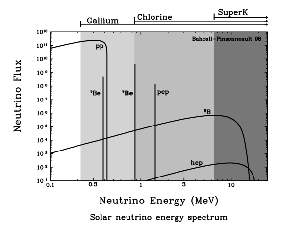
Figure 9: Energy generation in the Sun via the $pp$ chains (from ref. [18]).

Figure 10: Solar neutrino spectrum and thresholds of solar neutrino experiments as indicated above the figure (from ref. [48]).

The calculated fluxes of different components of the solar $\nu_{e}$ flux depend not only on the general principles laid in the basis of the standard solar models, but also on a number of input parameters, such as the solar opacity and various nuclear cross sections. These parameters are known to a varying degree of accuracy [48]. The flux of the most abundant $pp$ neutrinos is closely related to the well known luminosity of the sun, and therefore has a very small uncertainty, $\sim 1\%$. On the other hand, the flux of the energetic ⁸B neutrinos has a relatively large uncertainty, $\sim 20\%$. The flux of the most energetic $hep$ neutrinos is the least certain one – it is only known to an accuracy of 1 - 2 orders of magnitude. Fortunately, this flux is very small, and its contribution to the detection rates of solar neutrinos is practically negligible. It can, however, affect the high energy part of the solar neutrino spectrum.

The solar neutrinos have been detected in five solar neutrino experiments. Historically, the first one was the Homestake experiment of Davis and his collaborators. It is based on the reaction

$$\nu_{e}+{\rm{}^{37}Cl}\to{\rm{}^{37}Ar}+e^{-}\,.$$ (129)

The radioactive argon atoms produced in this reaction are extracted using chemical methods and counted in proportional counters. The energy threshold of reaction (129) is 0.814 MeV, so only the ⁸B and ⁷Be and $pep$ neutrinos are detected in the Homestake experiment, the largest contribution coming from the ⁸B neutrinos (see figs. 10 and 12). Radiochemical techniques are also used in two other solar neutrino experiments – SAGE and Gallex, in which the reaction

$$\nu_{e}+{\rm{}^{71}Ga}\to{\rm{}^{71}Ge}+e^{-}\,.$$ (130)

is employed. The energy threshold of this reaction is 0.234 MeV, and so the gallium experiments can also detect the lowest energy $pp$ neutrinos. Since the flux of the $pp$ neutrinos is very large, they are expected to give the main contribution to the event rates in the SAGE and Gallex detectors (fig. 12). The remaining two experiments – Kamiokande and its up-scaled version Super-Kamiokande – are the water Cherenkov detectors and use the neutrino-electron scattering reaction

$$\nu_{a}+e^{-}\to\nu_{a}+e^{-}\,.$$ (131)

to detect solar neutrinos. This reaction has zero physical threshold, but one has to introduce energy cuts to suppress the background. In the Kamiokande experiment solar neutrinos with the energies $E>7.5$ MeV were detected, whereas the threshold used by Super-Kamiokande is at present 5.5 MeV. With these energy cuts, the Kamiokande and Super-Kamiokande detection rates are only sensitive to the ⁸B component of the solar neutrino flux. Reaction (131) has a very interesting feature – for neutrino energies $E\gg m_{e}$ the angular distribution of the recoil electrons is forward-peaked, i.e. it points in the direction of the momentum of the incoming neutrino. The angular distributions of neutrinos detected in the Kamiokande and Super-Kamiokande experiments have a prominent peak at $180^{\circ}$ from the direction to the sun, which is a beautiful proof of the solar origin of these neutrinos. The origin of the neutrinos detected in the radiochemical experiments is unknown, and our belief that they come from the sun is based on the fact that no other sources of sufficient strength and energy are known.

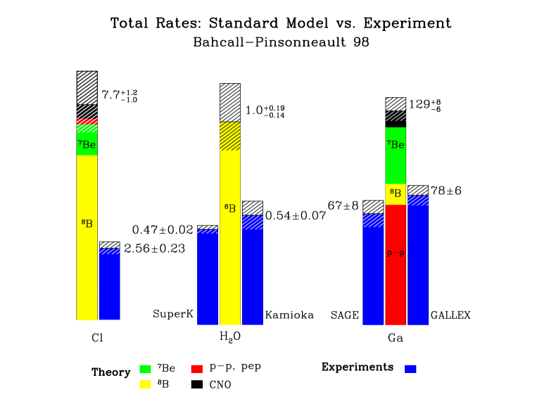
Figure 11: Predictions of standard solar models since 1988. The ⁷Be and ⁸B fluxes are normalized to the predictions of the BP98 model. The rectangular box defines the 3$\sigma$ error range of the BP98 model. The best-fit ⁷Be flux is negative (from ref. [49]).

Figure 12: Solar neutrino measurements and theoretical flux predictions. For Cl and Ga experiments, the units are SNU (1 SNU = $10^{-36}$ captures per target atom per second); for H₂O experiments, the ratio data/exp. is shown. From ref. [48].

In all five solar neutrino experiments, fewer neutrinos than expected were detected, the degree of deficiency being different in the experiments of different types (fig. 12). This is the essence of the solar neutrino problem. The observed deficiency of solar neutrinos could be due to an insufficient knowledge of solar physics or an error in some input parameters (astrophysical solution), or due to experiment-related errors (such as miscalculated detection efficiency or cross section), or due to some unknown neutrino physics (particle physics solution of the solar neutrino problem). As we have already discussed, the standard solar models are well grounded, agree with each other and with helioseismological observations. All the solar neutrino experiments but one (Homestake) have been calibrated, and their experimental responses were found to be in a very good agreement with expectations. The argon extraction efficiency of the Homestake detector was also checked by doping it with a known small number of radioactive argon atoms, but no calibration has been carried out since no artificial source of neutrinos with a suitable energy spectrum exists.

The solar neutrino problem is not just the problem of the deficit of the observed neutrino flux: results of different experiments seem to be inconsistent with each other. In the absence of new neutrino physics, the energy spectra of the various components of the solar neutrino flux are given by the standard nuclear physics and well known, and only the total fluxes of these components may be different from those predicted by the standard solar models. One can then infer the flux of ⁸B neutrinos directly from the Kamiokande or Super-Kamiokande data, and use this flux to find the corresponding contribution to the Homestake detection rate. This contribution turns out to be larger than the total detection rate, so the best-fit contribution of the ⁷Be neutrinos to the Homestake detection rate is negative! In fact, if one assumes that the solar neutrino spectra are undistorted, one can demonstrate the existence of the solar neutrino problem without using any information about solar physics except the solar luminosity constraint, or even without this constraint, i.e. in a solar-model independent way. Therefore the probability of the astrophysical solution of the solar neutrino problem is very low.

Alternatively, one could assume that the observed deficit of solar neutrinos is due to some unknown experimental errors. However, in this case it is not sufficient to assume that one of the solar neutrino experiments is wrong; one would have to assume that the experiments of at least two different types (chlorine, gallium and water Cherenkov) are wrong, which is very unlikely. The remaining possibility is that the spectra of solar neutrinos are distorted, which requires new neutrino physics.

There are several possible particle-physics solutions of the solar neutrino problem, the most natural one being neutrino oscillations (for an alternative solution related to nonzero neutrino magnetic moments, see e.g. [16]). The neutrino oscillation solution has become even more plausible after the strong evidence for atmospheric neutrino oscillations was reported by the Super-Kamiokande Collaboration. Neutrino oscillations can convert a fraction of solar $\nu_{e}$ into $\nu_{\mu}$ or $\nu_{\tau}$ (or their combination). Since the energy of solar neutrinos is smaller than the masses of muons and tauons, these $\nu_{\mu}$ or $\nu_{\tau}$ cannot be detected in the CC reactions of the type (129) or (130) and therefore are invisible in the chlorine and gallium experiments. They can scatter on electrons through the NC interactions and therefore should contribute to the detection rate in water Cherenkov detectors. However, the cross section of the NC channel of reaction (131) is about a factor of 6 smaller than that of the CC channel, and so the deficit of the neutrino flux observed in the Kamiokande and Super-Kamiokande experiments can be explained. The probabilities of neutrino oscillations depend on neutrino energy, and the distortion of the energy spectra of the experimentally detected solar neutrinos, which is necessary to reconcile the data of different experiments, is readily obtained.

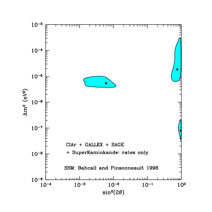
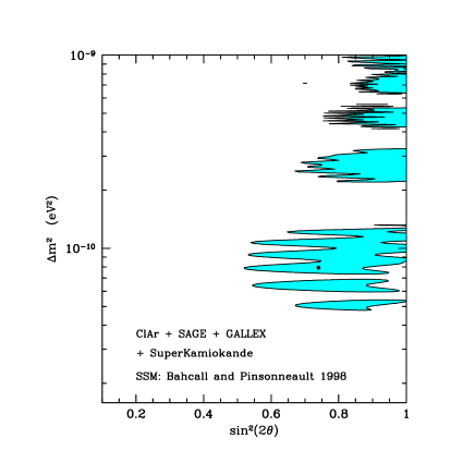
Figure 13: Left panel: Allowed regions (99 % c.l.) for the MSW solutions of the solar neutrino problem for 2-flavour oscillations of $\nu_{e}$ into active neutrinos (only rates included). Right panel: The same for the VO solution. From ref. [50].

The oscillations of solar neutrinos inside the sun can be strongly enhanced due to the MSW effect which we discussed in sec. 8, and the solar data can be fitted even with a very small vacuum mixing angle. Solar matter can also influence neutrino oscillations if the vacuum mixing angle is not small. The allowed values of the neutrino oscillation parameters $\sin^{2}2\theta_{0}$ and $\Delta m^{2}$ which fit the detection rates in the chlorine, gallium and water Cherenkov experiments in the 2-flavour scheme are shown in fig. 13 for matter enhanced (left panel) and vacuum (right panel) oscillations of $\nu_{e}$ into active neutrinos. In the case of the matter enhanced oscillations, there are three allowed ranges of the parameters corresponding to the small mixing angle (SMA), large mixing angle (LMA) and low $\Delta m^{2}$ (LOW) MSW solutions [50, 51]. The LOW solution has a very low probability and only exists at 99% c.l.. The vacuum oscillation (VO) solution corresponds to very small values of $\Delta m^{2}$, for which the neutrino oscillation length (61) for typical solar neutrino energies ($\sim$ a few MeV) is comparable to the distance between the sun and the earth. This solution is also known as “just so” oscillation solution. For $\nu_{e}\to\nu_{sterile}$ oscillations, there is only the SMA solution with the allowed region of parameters similar to that for oscillations into active neutrinos.

Solar neutrinos detected during night travel some distance inside the earth on their way to the detector, and their oscillations can be affected by the matter of the earth. In particular, a fraction of $\nu_{\mu}$ or $\nu_{\tau}$ produced as a result of the solar $\nu_{e}$ oscillations can be reconverted into $\nu_{e}$ by oscillations enhanced by the matter of the earth. This earth “regeneration” (or day/night) effect can be appreciable in the case of the LMA solution, but is expected to be very small in the case of the SMA solution. The day/night effects (and in general, the zenith angle dependence of the neutrino signal) can in principle be observed in real-time experiments, such as Super-Kamiokande.

In the case of the MSW solutions of the solar neutrino problem the neutrino state arriving at the earth is an incoherent superposition of the mass eigenstates $\nu_{1}$ and $\nu_{2}$ (see Problem 23 below). The probability $P_{SE}$ of finding a solar $\nu_{e}$ after it traverses the earth depends on the average $\nu_{e}$ survival probability in the sun $\bar{P}_{S}$:

$$P_{SE}=\bar{P}_{S}+\frac{1-2\bar{P}_{S}}{\cos 2\theta_{0}}\,(P_{2e}-\sin^{2}\theta_{0})\,.$$ (132)

Here $P_{2e}=P(\nu_{2}\to\nu_{e})$ is the probability of oscillations of the second mass eigenstate into electron neutrino inside the earth. It follows from this expression that the sign of the night-day asymmetry $(N-D)/(N+D)$ depends on whether $\bar{P}_{S}$ is larger or smaller than 1/2. For the LMA solution, $\bar{P}_{S}<1/2$, and the night-day asymmetry is expected to be positive. For the SMA solution, $\bar{P}_{S}$ for the Super-Kamiokande experiment is close to 1/2, and therefore the expected day/night effect is small. It can in principle be of either sign. The value measured in the Super-Kamiokande experiment is [52]

$$\frac{N}{D}-1=0.067\pm 0.033\,(stat.)\pm 0.013\,(syst.)\,,$$ (133)

i.e. shows an excess of the night-time flux at about 2$\sigma$. The zenith angle event dependence measured by the Super-Kamiokande shows a rather flat distribution of the excess of events over different night-time zenith angle bins. This is rather typical for the LMA solution whereas for the SMA solution one normally expects the excess (or deficiency) to be concentrated in the vertical upward bin with zenith angles $\theta$ in the range $-1<\cos\theta<-0.8$. Thus, the night-time zenith angle dependence and the overall night-day asymmetry (133) favour the LMA solution of the solar neutrino problem.

As we discussed before, oscillations of solar neutrinos in the 3-flavour scheme can be described through the effective two-flavour $\nu_{e}$ survival probability (see eq. (74) and Problem 20). For a recent detailed analysis of the solar neutrino oscillations in the 3-flavour framework, see [53].

Problem 22. Discuss effects of the solar and earth’s matter on the oscillations of solar neutrinos in the case of VO solution. Take into account that the matter densities $\rho_{sun}$ and $\rho_{earth}$ vary in the ranges 0 – 150 and 2.7 – 12.5 $g/cm^{3}$ respectively.

Problem 23. Show that in the case of the MSW solutions the solar neutrino flux arriving at the earth can be considered as an incoherent superposition of the neutrino mass eigenstates $\nu_{1}$ and $\nu_{2}$. Hint: consider the relative phase between $\nu_{1}$ and $\nu_{2}$ states acquired by neutrinos on their way from the sun to the earth. Assume that the energy resolution of the neutrino detector $\Delta E\buildrel>\over{{}_{\sim}}100$ keV.

Problem 24. Derive equation (132) for the probability of finding a solar $\nu_{e}$ after it crosses the earth during night. Hint: use the results of the previous problem.

Figure 14: Recoil electron energy spectrum in the Super-Kamiokande experiment along with typical predictions of SMA, LMA and VO solutions (from ref. [52]).

As we have already discussed, neutrino oscillations (both in matter and in vacuum) depend on neutrino energy and therefore should result in certain distortions of the spectrum of the detected solar neutrinos. One can obtain an information on the spectrum of incoming neutrinos by measuring the recoil electron spectrum in the reaction (131). This spectrum has been measured in the Super-Kamiokande experiment, and the results (along with the typical predictions of the LMA, SMA and VO solutions) are shown in fig. (14). In the absence of the neutrino spectrum distortion, the ratio of measured/expected electron spectrum presented in this figure should be a horizontal line. The characteristic feature of the measured spectrum is an excess of events in the region of high energies. The experimental errors are still too large to allow a clean discrimination between different solutions of the solar neutrino problem; however, the spectrum favours VO over the other solutions. Another possible explanation of the excess of the high energy events is that the flux of the highest-energy $hep$ neutrinos has been underestimated by about a factor of 20. Since the $hep$ flux is very poorly known, this is still a possibility.

At present, the situation with the solar neutrino data is somewhat confusing: different pieces of the data favour different solutions of the solar neutrino problem. The total rates are better fitted within the SMA solution, the night/day ratio prefers the LMA solution, and the electron recoil spectrum in Super-Kamiokande favours the VO solution. Clearly, more data are needed to clear the situation up. Fortunately, two new experiments which can potentially resolve the problem are now under way or will soon be put into operation. The SNO (Sudbury Neutrino Observatory) experiment has started taking data, and its first results are expected some time during 2000. The Borexino experiment is scheduled to start data taking in 2001.

The SNO detector consists of 1000 tons of heavy water, and it detects solar neutrinos in three different channels:

$$\nu_{e}+d\to p+p+e^{-}\quad\quad({\rm CC}),~{}~{}E_{min}=1.44~{}{\rm MeV}\,,$$ (134)

$$\nu_{a}+d\to p+n+\nu_{a}\quad\quad({\rm NC}),~{}~{}E_{min}=2.23~{}{\rm MeV}\,,$$ (135)

and $\nu_{a}e$ scattering process (131) which can proceed through both CC and NC channels. The CC reaction (134) is very well suited for measuring the solar neutrino spectrum. Unlike in the case of $\nu_{a}e$ scattering (131) in which the energy of incoming neutrino is shared between two light particles in the final state, the final state of the reaction (134) contains only one light particle – electron, and a heavy $2p$ system whose kinetic energy is very small. Therefore by measuring the electron energy one can directly measure the spectrum of the solar neutrinos. Detecting the solar neutrino spectrum would be of great importance since any deviation from the spectrum predicted by the nuclear beta decay would be a “smoking gun” signature of new neutrino physics.

The cross section of the NC reaction (135) is the same for neutrinos of all three flavours, and therefore oscillations between $\nu_{e}$ and $\nu_{\mu}$ or $\nu_{\tau}$ would not change the NC detection rate in the SNO experiment. On the other hand, these oscillations would deplete the solar $\nu_{e}$ flux, reducing the CC event rate. Therefore the CC/NC ratio is a sensitive probe of neutrino flavour oscillations. If solar $\nu_{e}$ oscillate into electroweak singlet (sterile) neutrinos, both CC and NC event rates will be suppressed.

The Borexino experiment will detect solar neutrinos through the $\nu_{a}e$ scattering with a very low energy threshold, and will be able to detect the ⁷Be neutrino line. Different solutions of the solar neutrino problem predict different degree of suppression of ⁷Be neutrinos, and their detection could help discriminate between these solutions. Observation of the ⁷Be neutrino line would be especially important in the case of the VO solution. Due to the eccentricity of the earth’s orbit the distance between the sun and the earth varies by about 3.5% during the year, and this should lead to varying oscillation phase (and therefore varying solar neutrino signal) in the case of vacuum neutrino oscillations. This seasonal variation can in principle be separated from the trivial 7% variation due to the $1/L^{2}$ law which is not related to neutrino oscillations. However, the oscillation phase depends on neutrino energy [see (59)], and integration over significant energy intervals may make it difficult to observe the seasonal variations of the solar neutrino flux due to the VO. The ⁷Be neutrinos are monochromatic, which should facilitate the observation of the seasonal variations. The oscillation phase in (59) depends on the ratio $L/E$, therefore for neutrinos with continuous spectrum VO should lead to seasonal variations of the spectrum distortion which are correlated with the seasonal variations of the flux [54]. Such variations would be a clear signature of the VO solution.

Although up to now the sensitivities of the solar neutrino experiments have been insufficient to allow a clear-cut discrimination between different solutions of the solar neutrino problem, one can hope that the combined data of the currently operating and forthcoming experiments will allow to finally resolve the solar neutrino problem.

11 Atmospheric neutrinos

Atmospheric neutrinos are electron and muon neutrinos and their antineutrinos which are produced in the hadronic showers induced by primary cosmic rays in the earth’s atmosphere. The main mechanism of production of the atmospheric neutrinos is given by the following chain of reactions:

$$\begin{array}[]{lllll}p(\alpha,...)+Air&\rightarrow&\pi^{\pm}(K^{\pm})&+&X\\ &&\pi^{\pm}(K^{\pm})&\rightarrow&\mu^{\pm}+\nu_{\mu}(\bar{\nu}_{\mu})\\ &&&&\mu^{\pm}\rightarrow e^{\pm}+\nu_{e}(\bar{\nu}_{e})+\bar{\nu}_{\mu}(\nu_{\mu})\end{array}$$ (136)

Atmospheric neutrinos can be observed directly in large mass underground detectors predominantly by means of their CC interactions:

$$\nu_{e}(\bar{\nu}_{e})+A\rightarrow e^{-}(e^{+})+X\,,$$

$$\nu_{\mu}(\bar{\nu}_{\mu})+A\rightarrow\mu^{-}(\mu^{+})+X\,.$$ (137)

Naively, from the reaction chain (136) one would expect to have two atmospheric muon neutrinos or antineutrinos for every electron neutrino or antineutrino. In reality, the situation is more complicated: one should take into account the differences in the lifetimes of $\pi^{\pm}$, $K^{\pm}$ and $\mu^{\pm}$ as well as the differences in their spectra. Also, although the reaction chain (136) is the dominant source of atmospheric neutrinos, it is not the only one. Calculations of the atmospheric neutrino fluxes predict the $\nu_{\mu}/\nu_{e}$ ratio that depends on neutrino energy and the zenith angle of neutrino trajectory, approaching 2 for low energy neutrinos and horizontal trajectories but exceeding this value for higher energy neutrinos and for trajectories close to vertical.

Accurate calculation of the atmospheric neutrino fluxes is a difficult job which includes such ingredients as spectra and chemical composition of cosmic rays (including geomagnetic effects and solar activity), cross sections of $\pi$ and $K$ production off the nuclear targets, Monte Carlo simulation of hadronic cascades in the atmosphere and the calculation of neutrino spectra including muon polarization effects. Each step introduces some uncertainty in the calculation. The overall uncertainty of the calculated atmospheric neutrino fluxes is rather large, and the total fluxes calculated by different authors differ by as much as 20 – 30%. At the same time, the ratio of the muon to electron neutrino fluxes is fairly insensitive to the above uncertainties, and different calculations yield the ratios of muon-like to electron-like contained events which agree to about 5%. This ratio has been measured in a number of experiments, and the Kamiokande and IMB Collaborations reported smaller than expected ratio in their contained events, with the double ratio $R(\mu/e)\equiv[(\nu_{\mu}+\bar{\nu}_{\mu})/(\nu_{e}+\bar{\nu}_{e}]_{data}/[(\nu_{\mu}+\bar{\nu}_{\mu})/(\nu_{e}+\bar{\nu}_{e})]_{MC}\simeq 0.6$ where MC stands for Monte Carlo simulations. The discrepancy between the observed and predicted atmospheric neutrino fluxes was called the atmospheric neutrino anomaly. The existence of this anomaly was subsequently confirmed by Soudan 2, MACRO and Super-Kamiokande experiments. Most remarkably, the Super-Kamiokande (SK) Collaboration obtained a very convincing evidence for the up-down asymmetry and zenith-angle dependent deficiency of the flux of muon neutrinos, which has been interpreted as an evidence for neutrino oscillations. We shall now discuss the SK data and their interpretation.

The SK detector is a 50 kt water Cherenkov detector (22.5 kt fiducial volume) which is overseen by more than 13,000 photomultiplier tubes. The charged leptons born in the CC interactions of neutrinos produce the rings of the Cherenkov light in the detector which are observed by the phototubes. Muons can be distinguished from electrons since their Cherenkov rings are sharp whereas those produced by electrons are diffuse. The SK Collaboration subdivided their atmospheric neutrino events into several groups, depending on the energy of the charged leptons produced. Fully contained (FC) events are those for which the neutrino interaction vertex is located inside the detector and all final state particles do not get out of it. FC events are further subdivided into sub-GeV (visible energy $<1.33$ GeV) and multi-GeV (visible energy $>1.33$ GeV) events. Partially contained (PC) events are those for which the produced muon exits the inner detector volume (only muons are penetrating enough). The average energy of a neutrino producing a PC event in SK is $\sim 15$ GeV. Muon neutrinos can also be detected indirectly by observing the muons that they have produced in the material surrounding the detector. To reduce the background from atmospheric muons, only upward–going neutrino-induced muons are usually considered. A rough estimate of the energy spectrum of the upward–going muons has been obtained dividing them in two categories, passing (or through-going) and stopping muons. The latter, which stop inside the detector, correspond to the average parent neutrino energy $\sim 10$ GeV, whereas for the through-going muons the average neutrino energy is $\sim 100$ GeV.

The measurements of the double ratio $R(\mu/e)$ for contained events at SK (848 live days) give [3]

$$R=0.68\pm 0.02\,(stat.)\pm 0.05\,(syst.)\quad\mbox{(sub-GeV)}\,,$$

$$R=0.68\pm 0.04\,(stat.)\pm 0.08\,(syst.)\quad\mbox{(multi-GeV)}\,.$$ (138)

The value of $R$ for sub-GeV events is different from unity (to which it should be equal in no-oscillation case) by $5.9\sigma$.

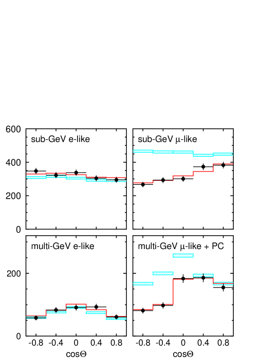
Figure 15: Zenith angle distributions for sub-GeV and multi-GeV e-like and $\mu$-like events at SK. The bars show the (no-oscillations) Monte Carlo predictions; the lines show the predictions for $\nu_{\mu}\leftrightarrow\nu_{\tau}$ oscillations with the best-fit parameters $\Delta m^{2}=3.5\times 10^{-3}$ eV², $\sin^{2}2\theta=1.0$. From [55].

We shall now discuss the zenith angle distributions of the atmospheric neutrino events. It should be remembered that the zenith angle distributions of the charged leptons which are experimentally measured do not coincide with those of their parent neutrinos: for multi-GeV neutrinos the average angle between the momenta of neutrinos and charged leptons is about $17^{\circ}$, whereas for sub-GeV neutrinos it is close to $60^{\circ}$. This is properly taken into account in MC simulations. For PC events and upward going muons the correlation between the directions of momenta of muons and parent neutrinos is much better. The distances $L$ traveled by neutrinos before they reach the detector vary in a wide range: for vertically downward going neutrinos (neutrino zenith angle $\theta_{\nu}=0$) $L\sim 15$ km; for horizontal neutrino trajectories ($\theta_{\nu}=90^{\circ}$) $L\sim 500$ km; the vertically up-going neutrinos ($\theta_{\nu}=180^{\circ}$) cross the earth along its diameter and for them $L\sim 13,000$ km.

In fig. 15 the zenith angle distributions of the SK e-like and $\mu$-like events are shown separately for sub-GeV and multi-GeV contained events. The data correspond to 736 live days. (By the time these lecture notes were being written, the results for 848 live days of data taking had been reported, but no high-quality figures for zenith angle distributions were publicly available). One can see that for e-like events, the measured zenith angle distributions agree very well with the MC predictions (shown by bars), both in the sub-GeV and multi-GeV samples, while for $\mu$-like events both samples show zenith-angle dependent deficiency of event numbers compared to expectations. The deficit of muon neutrinos is stronger for upward going neutrinos which have larger pathlengths. In the multi-GeV sample, there is practically no deficit of events caused by muon neutrinos coming from the upper hemisphere ($\cos\theta>0$), whereas in the sub-GeV sample, all $\mu$-like events exhibit a deficit which decreases with $\cos\theta$. This pattern is perfectly consistent with oscillations $\nu_{\mu}\leftrightarrow\nu_{\tau}$ or $\nu_{\mu}\leftrightarrow\nu_{s}$ where $\nu_{s}$ is a sterile neutrino. Muon neutrinos responsible for the multi-GeV sample are depleted by the oscillations when their pathlength is large enough; the depletion becomes less pronounced as the pathlength decreases ($\cos\theta$ increases); for neutrinos coming from the upper hemisphere, the pathlengths are too short and there are practically no oscillations. Neutrinos responsible for the sub-GeV $\mu$-like events have smaller energies, and so their oscillation lengths are smaller; therefore even neutrinos coming from the upper hemisphere experience sizeable depletion due to the oscillations. For up-going sub-GeV neutrinos the oscillation length is much smaller than the pathlength and they experience averaged oscillations. The solid line in fig. 15 obtained with the $\nu_{\mu}\leftrightarrow\nu_{\tau}$ oscillation parameters in the 2-flavour scheme $\Delta m^{2}=3.5\times 10^{-3}$ eV², $\sin^{2}2\theta=1.0$ gives an excellent fit of the data.

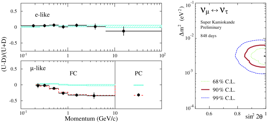
Figure 16: Left panel: up-down asymmetry vs event momentum for single ring e-like and $\mu$-like events in SK. Right panel: SK allowed regions for oscillations parameters for $\nu_{\mu}\leftrightarrow\nu_{\tau}$ channel in 2-flavour scheme (FC + PC single ring events). From [3].

An informative parameter characterizing the distortion of the zenith angle distribution is the up-down asymmetry $A$, where up corresponds to the events with $\cos\theta<-0.2$ and down to those with $\cos\theta>0.2$. The flux of atmospheric neutrinos is expected to be nearly up-down symmetric for neutrino energies $E\buildrel>\over{{}_{\sim}}1$ GeV, with minor deviations coming from geomagnetic effects which are well understood and can be accurately taken into account. In particular, at the geographical location of the SK detector small positive asymmetry is expected. Any significant deviation of the up-down asymmetry of neutrino induced events from the asymmetry due to the geomagnetic effects is an indication of neutrino oscillations or some other new neutrino physics. The asymmetry measured for the SK multi-GeV $\mu$-like events is [3]

$$A=\frac{U-D}{U+D}=-0.32\pm 0.04\,(stat.)\pm 0.01\,(syst.)\,,$$ (139)

i.e. is negative and differs from zero by almost $8\sigma$! The dependence of the asymmetries for e-like FC and $\mu$-like FC+PC events on the event momentum is shown in fig. 16 (left panel). One can see that for e-like events $A\simeq 0$ for all momenta. At the same time, for $\mu$-like events the asymmetry is close to zero at low momenta and decreases with momentum. This is easily understood in terms of the $\nu_{\mu}$ oscillations. For very small momenta, the oscillation length is small and both up-going and down-going neutrino fluxes are depleted by oscillations to about the same extent; in addition, loose correlation between the directions of the momenta of the charged lepton and of its patent neutrino tends to smear out the asymmetry at low energies. With increasing momentum the oscillation length increases, and the pathlength of down-going neutrinos becomes too small for oscillations to develop. The right panel of fig. 16 gives the allowed values of the oscillation parameters following from the SK FC and PC event data. The best fit corresponds to $\Delta m^{2}=3.1\times 10^{-3}$ eV², $\sin^{2}2\theta=0.99$ and has a very good $\chi^{2}/d.o.f.=55/67$. In this analysis the poorly known overall normalization factor of the neutrino flux was considered as a free parameter, and the best fit was achieved with 5% upward renormalization of the flux of Honda et al. [56]. The above value of $\chi^{2}$ should be compared with that of the no-oscillation hypothesis: $\chi^{2}/d.o.f.=177/69$, which is a very poor fit.

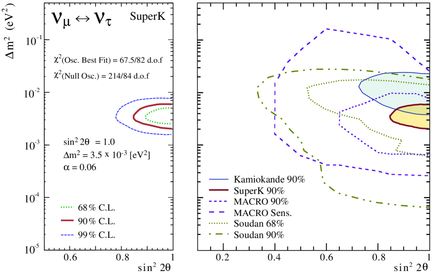
Figure 17: Left panel: SK allowed regions of oscillation parameters for $\nu_{\mu}\leftrightarrow\nu_{\tau}$ channel in 2-flavour scheme (FC + PC single ring events + upward through-going + upward stopping events). Right panel: comparison of allowed values of oscillation parameters obtained in different experiments. From [3].

The SK data show evidence for neutrino oscillations not only in their FC and PC $\mu$-like events: upward stopping and upward through-going events also demonstrate zenith angle dependent deficiency of muon neutrinos consistent with neutrino oscillations, although the statistics for up-going muons is lower than that for contained events. Fig. 17 (left panel) summarizes the allowed region for 2-flavour neutrino oscillations obtained from the combined analysis of the SK FC and PC single ring events (848 live days), upward through-going (923 live days) and upward stopping events (902 live days). The best fit ($\chi^{2}/d.o.f=67.5/82$) was obtained for $\Delta m^{2}=3.5\times 10^{-3}$ eV², $\sin^{2}2\theta=1.0$ and the upward 6% renormalization of the flux of Honda et al. The no-oscillation fit gives $\chi^{2}/d.o.f.=214/84$. The right panel gives the comparison of the allowed regions obtained in different atmospheric neutrino experiments. The evidence for neutrino oscillations is very impressive.

Are neutrino oscillations that are responsible for the depletion of the $\nu_{\mu}$ flux $\nu_{\mu}\leftrightarrow\nu_{\tau}$ or $\nu_{\mu}\leftrightarrow\nu_{s}$? For contained events, the oscillation probabilities in these two channels are nearly the same and the data can be fitted equally well in both cases, with very similar allowed ranges of the oscillation parameters. However, for higher energy upward going events there are important differences between these two cases. In the 2-flavour scheme, $\nu_{\mu}\leftrightarrow\nu_{\tau}$ oscillations are not affected by matter because the interactions of $\nu_{\mu}$ and $\nu_{\tau}$ with matter are identical. However, sterile neutrinos do not interact with matter at all, and therefore the $\nu_{\mu}\leftrightarrow\nu_{s}$ oscillations are affected by the matter-induced potential $V_{\mu}-V_{s}=V_{\mu}$. At low energies, the kinetic energy difference $\Delta m^{2}/2E$ dominates over $V_{\mu}$, and the earth’s matter effects are unimportant. They become important at higher energies, when $\Delta m^{2}/2E\sim V_{\mu}$; at very high energies, when $\Delta m^{2}/2E\ll V_{\mu}$, matter strongly suppresses neutrino oscillations both in $\nu_{\mu}\leftrightarrow\nu_{s}$ and $\bar{\nu}_{\mu}\leftrightarrow\bar{\nu}_{s}$ channels (see eq. (97) where $N_{e}$ has to be replaced by $\mp N_{n}/2$ for these oscillation channels). Therefore the oscillations of high energy neutrinos travelling significant distances in the earth should be strongly suppressed in this case.

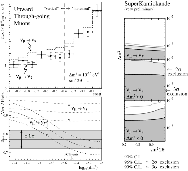
Figure 18: Left top panel: Zenith angle distribution of upward through-going events at SK. The dashed and short-dashed histograms show the $\nu_{\mu}\leftrightarrow\nu_{\tau}$ and $\nu_{\mu}\leftrightarrow\nu_{s}$ solutions respectively. Left bottom: Vertical/Horizontal ratio for upward through-going muons along with the predictions of $\nu_{\mu}\leftrightarrow\nu_{\tau}$ and $\nu_{\mu}\leftrightarrow\nu_{s}$ oscillation scenarios. Right panel: Exclusion regions obtained from Up/Down ratio for energetic PC sample ($E_{vis}>5$ GeV, $\langle E\rangle\sim 25$ GeV) and Vertical/Horizontal ratio for upward through-going events. From [3].

Fig. 18 (upper left panel) shows the zenith angle distribution of the upward through-going events ($\langle E\rangle\sim 100$ GeV) along with the predictions of $\nu_{\mu}\leftrightarrow\nu_{\tau}$ and $\nu_{\mu}\leftrightarrow\nu_{s}$ scenarios with parameters obtained from the fits of contained events. It can be seen that the $\nu_{\mu}\leftrightarrow\nu_{\tau}$ oscillation channel describes the “vertical” ($\cos\theta<-0.4$) events better than the $\nu_{\mu}\leftrightarrow\nu_{s}$ channel. For horizontal and nearly horizontal events ($-0.4<\cos\theta<0$) both scenarios give similar predictions since the neutrinos do not travel inside the earth or travel only small distances there. This is further illustrated by the left bottom panel of fig. 18 in which the Vertical/Horizontal event ratio is plotted. The excluded ranges of the oscillation parameters for various oscillation channels are shown in the right panel of fig. 18. One can conclude that the $\nu_{\mu}\leftrightarrow\nu_{s}$ oscillations are currently disfavoured at the $2\sigma$ level, although not yet completely ruled out as a possible solution of the atmospheric neutrino problem.

Another way to discriminate between $\nu_{\mu}\leftrightarrow\nu_{\tau}$ and $\nu_{\mu}\leftrightarrow\nu_{s}$ as the two possible main channels of the atmospheric neutrino oscillations is through the detection of single pions produced in the NC reactions $\nu N\to\nu N\pi^{0}$. Sterile neutrinos do not participate in these reactions and therefore $\nu_{\mu}\leftrightarrow\nu_{s}$ oscillations would deplete the number of the observed $\pi^{0}$’s. Unfortunately, cross sections of these NC reactions are only known with large uncertainties, and at the moment a clear discrimination between the $\nu_{\mu}\leftrightarrow\nu_{\tau}$ and $\nu_{\mu}\leftrightarrow\nu_{s}$ oscillations of atmospheric neutrinos through the detection of single neutral pions does not seem to be possible. The situation may change in the near future, however, as the K2K Collaboration is planning to perform high statistics measurements of neutrino interactions in their near detector.

Can $\nu_{\mu}\leftrightarrow\nu_{e}$ oscillations be responsible for the observed anomalies in the atmospheric neutrino data? The answer is no, at least not as the dominant channel. Explaining the data requires oscillations with large mixing equal or close to the maximal one; $\nu_{\mu}\leftrightarrow\nu_{e}$ oscillations would then certainly lead to a significant distortion of the zenith angle distributions of the e-like contained events, contrary to observations. In addition, for $\Delta m^{2}$ in the range $\sim 10^{-3}$ eV² which is required by the atmospheric neutrino data, $\nu_{\mu}\leftrightarrow\nu_{e}$ oscillations are severely restricted by the CHOOZ reactor antineutrino experiment, which excludes these oscillations as the main channel of the atmospheric neutrino oscillations (see sec. 12).

However, $\nu_{\mu}\leftrightarrow\nu_{e}$ and $\nu_{e}\leftrightarrow\nu_{\tau}$ can be present as subdominant channels of the oscillations of atmospheric neutrinos. This may lead to interesting matter effects on oscillations of neutrinos crossing the earth on their way to the detector. Matter can strongly affect $\nu_{e}\leftrightarrow\nu_{\mu,\tau}$ and $\bar{\nu}_{e}\leftrightarrow\bar{\nu}_{\mu,\tau}$ oscillations leading to an enhancement of the oscillation probabilities for neutrinos and suppression for antineutrinos or vice versa, depending on the sign of the corresponding mass squared difference. For certain neutrino energies, one can expect an enhancement due to the MSW effect in the mantle or in the core of the earth. In addition, there can be a specific enhancement effect, different from the MSW one, due to a cumulative build-up of the transition probability for neutrinos crossing the earth’s mantle, core and then again mantle (parametric resonance [42, 43, 44, 37]). The matter enhancement effects are expected to take place in a relatively narrow range of neutrino energies, and it is rather difficult to observe them experimentally. Yet the possibility of the observation of matter effects on oscillations of atmospheric neutrinos is very exciting.

Since three neutrino flavours are known to exist, oscillations of atmospheric neutrinos should in general be considered in the full 3-flavour framework (assuming that no sterile neutrinos take part in these oscillations). As follows from the analyses of solar and atmospheric neutrino data, there should be two distinct mass squared difference scales in the three neutrino framework, $\Delta m^{2}_{atm}\sim 10^{-3}\,\mbox{eV}^{2}$ and $\Delta m^{2}_{\odot}\buildrel<\over{{}_{\sim}}10^{-4}\,\mbox{eV}^{2}$. The hierarchy $\Delta m^{2}_{atm}\gg\Delta m_{\odot}^{2}$ means that one of the three neutrino mass eigenstates (which we denote $\nu_{3}$) is separated by the larger mass gap from the other two. The neutrino mass squared differences thus satisfy $|\Delta m_{31}|^{2}\simeq|\Delta m_{32}|^{2}\gg|\Delta m_{21}|^{2}$. We know already that $\nu_{\mu}\leftrightarrow\nu_{\tau}$ should be the main channel of oscillations whereas $\nu_{e}\leftrightarrow\nu_{\mu,\tau}$ oscillations can only be present as the subdominant channels. In the 3-flavour framework this means that the element $|U_{e3}|$ of the lepton mixing matrix (64) is small. The smallness of $|U_{e3}|$ means that the $\nu_{\mu}\leftrightarrow\nu_{\tau}$ and $\nu_{\mu}\leftrightarrow\nu_{e}$ oscillations approximately decouple, and the 2-flavour analysis gives a good first approximation. In terms of the parametrization (65) of the lepton mixing matrix, the mixing angle describing the main channel of the atmospheric neutrino oscillations is $\theta_{23}$, and its best-fit value following from the SK data is $45^{\circ}$. This fact and the smallness of $|U_{e3}|=s_{13}$ mean that the mass eigenstate $\nu_{3}$ mainly consists of the flavour eigenstates $\nu_{\mu}$ and $\nu_{\tau}$ with approximately equal weights, while the admixture of $\nu_{e}$ to this state is small or zero.

Can one observe true 3-flavour effects in the atmospheric neutrino oscillations? In principle, yes. Although in the 2-flavour scheme $\nu_{\mu}\leftrightarrow\nu_{\tau}$ oscillations are not affected by matter, in the full 3-flavour approach these oscillations are modified by matter because of the mixing with $\nu_{e}$. These matter effects are, however, rather small because of the smallness of $|U_{e3}|$. Three-flavour effects can also lead to interesting phenomena in the subdominant $\nu_{\mu}\leftrightarrow\nu_{e}$ and $\nu_{e}\leftrightarrow\nu_{\tau}$ oscillations. To see this, let us consider the fluxes $F_{\mu}$ and $F_{e}$ of atmospheric $\nu_{\mu}$ and $\nu_{e}$ in the presence of oscillations. As we discussed in sec. 8.4, in the case of the hierarchy $|\Delta m_{31}|^{2}\simeq|\Delta m_{32}|^{2}\gg|\Delta m_{21}|^{2}$ the oscillation probabilities in the 3-flavour scheme simplify significantly and can be expressed through the evolution matrix of the effective 2-flavour problem. Using eqs. (119) - (123) one can express $F_{\mu}$ and $F_{e}$ through the corresponding no-oscillation fluxes $F_{\mu}^{0}$ and $F_{e}^{0}$ as

$$F_{e}=F_{e}^{0}\left[1+P_{2}(rs_{23}^{2}-1)\right]\,,$$ (140)

$$F_{\mu}=F_{\mu}^{0}\left[1-s_{23}^{4}\left(1-\frac{1}{rs_{23}^{2}}\right)P_{2}+2s_{23}^{2}c_{23}^{2}\left(Z\cos\Phi+W_{3}\sin\Phi-1\right)\right],$$ (141)

where $r(E,\theta_{\nu})=F_{\mu}^{0}(E,\theta_{\nu})/F_{e}^{0}(E,\theta_{\nu})$. It is interesting that the subdominant $\nu_{e}\leftrightarrow\nu_{\mu,\tau}$ oscillations may lead either to an excess or to a deficiency of e-like events depending on the values of $r$ and $s_{23}$. Indeed, the effect of oscillations on the electron neutrino flux is proportional to the factor $(rs_{23}^{2}-1)$. If one assumes $r=2$, there will be an excess of e-like events for $\theta_{23}>45^{\circ}$ and a deficiency for $\theta_{23}<45^{\circ}$. The SK best fit is $\theta_{23}=45^{\circ}$; for this value of $\theta_{23}$ there would be no deviation from the prediction for $r=2$. However, for upward going neutrinos in the multi-GeV range $r$ is typically 3 – 3.5 rather than 2, so there should be an excess of e-like events for $\theta_{23}\buildrel>\over{{}_{\sim}}33^{\circ}$ and a deficiency for $\theta_{23}\buildrel<\over{{}_{\sim}}33^{\circ}$. Thus, the distortions of the zenith angle distributions of the e-like events due to the subdominant $\nu_{e}\leftrightarrow\nu_{\mu,\tau}$ oscillations should depend on the value of the mixing angle $\theta_{23}$ governing the dominant $\nu_{\mu}\leftrightarrow\nu_{\tau}$ oscillation channel. However, these distortions are expected to be small because of the smallness of $|U_{e3}|$ (notice that the probability $P_{2}$ in (140) and (141) vanishes in the limit $U_{e3}\to 0$). For recent analyses of the SK atmospheric neutrino data in the 3-flavour framework, see [57, 37].

If the solution of the solar neutrino problem is the LMA MSW effect, $\Delta m_{21}^{2}$ can be as large as $\sim 10^{-4}$ eV² and its influence of the atmospheric neutrino oscillations cannot be neglected. In that case eqs. (140) and (141) have to be modified. It was shown in [58] that in this case the subdominant oscillations can lead to a negative up-down asymmetry of e-like events at relatively large momenta. If the trend of slightly decreasing with momentum asymmetry of the e-like events which can be seen in the left top panel of fig. 16 is of physical origin and not just due to statistical fluctuations, it can be explained by relatively large $\Delta m_{21}^{2}$.

Are the standard neutrino oscillations the sole possible explanation of the observed atmospheric neutrino anomalies? In principle, other explanations are possible. Those include exotic types of neutrino oscillations – matter-induced oscillations due to flavour-changing interactions of neutrinos with medium [59], oscillations due to small violations of the Lorentz or CPT invariance or of the gravitational equivalence principle [60], and also neutrino decay [61]. Exotic oscillations lead to periodic variations of the $\nu_{\mu}$ survival probability with the oscillation lengths $l_{osc}\propto E^{-n}$ where $n=0$ in the case of flavour-changing neutrino interactions or violation of CPT invariance, and $n=1$ for oscillations due to the violations of the Lorentz invariance or equivalence principle. This has to be contrasted with $n=-1$ in the case of the standard neutrino oscillations. The energy dependence of the oscillation length can be tested in the atmospheric neutrino experiments as the energies of detected neutrinos span more than 3 orders of magnitude. The analysis was performed in [62], and the authors found that the fit of the atmospheric neutrino data assuming oscillations with $l_{osc}\propto E^{-n}$ gives $n=-0.9\pm 0.4$ at 90% c.l.. This clearly favours the standard oscillations over the exotic ones. In contrast to this, the neutrino decay mechanism fits the SK data quite well, the quality of the fit being as good as the one for the standard neutrino oscillations [63]. However, the assumed neutrino decay mode (into a sterile neutrino and a Majoron) requires particle physics models which look less appealing than those that provide neutrino masses required for the standard neutrino oscillations.

Problem 25. Using eqs. (119) - (123) of sec. 8.4 derive expressions (140) and (141) for the atmospheric $\nu_{e}$ and $\nu_{\mu}$ fluxes in the presence of oscillations in the case of the hierarchy $|\Delta m_{31}|^{2}|\simeq\Delta m_{32}|^{2}\gg|\Delta m_{21}|^{2}$.

12 Reactor and accelerator neutrino experiments

In reactor neutrino experiments oscillations of electron antineutrinos into another neutrino species are searched for by studying possible depletion of the $\bar{\nu}_{e}$ flux beyond the usual geometrical one [64, 65]. These are the disappearance experiments, because the energies of the reactor $\bar{\nu}_{e}$’s ($\langle E\rangle\simeq$ 3 MeV) are too small to allow the detection of muon or tauon antineutrinos in CC experiments. Small $\bar{\nu}_{e}$ energy makes the reactor neutrino experiments sensitive to oscillations with rather small values of $\Delta m^{2}$.

         

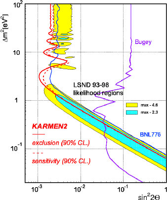
Figure 19: Left panel: CHOOZ exclusion region for $\bar{\nu}_{e}\to\bar{\nu}_{x}$ oscillations. The region to the right of the curves are excluded. Shaded areas correspond to the Kamiokande allowed region for atmospheric $\nu_{\mu}\to\nu_{e}$ oscillations [66]. Right panel: LSND allowed region for $\bar{\nu}_{\mu}\to\bar{\nu}_{e}$ oscillations (shaded areas) along with KARMEN, BNL776 and Bugey exclusion regions [65].

Up to now, no evidence for neutrino oscillations has been found in the reactor neutrino experiments, which allowed to exclude certain regions in the neutrino parameter space. The best constraints were obtained by the CHOOZ experiment in France [66] (see fig. 19). As follows from eq. (72), in the case of the hierarchy $\Delta m_{31}^{2}\simeq\Delta m_{32}^{2}\gg\Delta m_{21}^{2}$, the survival probability of $\nu_{e}$ (which by CPT invariance is equal to that of $\bar{\nu}_{e}$) in the 3-flavour scheme has a simple form which coincides with that in the two-flavour framework. Therefore the excluded regions obtained in the 2-flavour analysis apply to the 3-flavour case as well, with the identification $\Delta m^{2}=\Delta m_{31}^{2}\simeq\Delta m_{32}^{2}$, $\sin^{2}2\theta=\sin^{2}2\theta_{13}$. For the values of $\Delta m_{31}^{2}\equiv\Delta m_{atm}^{2}$ in the Super-Kamiokande allowed region $(2-6)\cdot 10^{-3}$ eV², the CHOOZ results give the following constraint on the element $U_{e3}$ of the lepton mixing matrix: $|U_{e3}|^{2}(1-|U_{e3}|^{2})<0.045-0.02$, i.e. $|U_{e3}|$ is either small or close to unity. The latter possibility is excluded by solar and atmospheric neutrino observations, and one finally obtains

$$\sin^{2}\theta_{13}\equiv|U_{e3}|^{2}\leq(0.047-0.02)\,\quad{\rm for}\quad\Delta m_{31}^{2}=(2-6)\cdot 10^{-3}~{}{\rm eV}^{2}\,.$$ (142)

This is the most stringent constraint on $|U_{e3}|$ to date.

Presently, a long baseline reactor experiment KamLAND is under construction in Japan. This will be a large liquid scintillator detector experiment using the former Kamiokande site. KamLAND will detect electron antineutrinos coming from several Japanese power reactors at an average distance of about 180 km. KamLAND is scheduled to start taking data in 2001 and will be sensitive to values of $\Delta m^{2}$ as low as $4\times 10^{-6}$ eV², i.e. in the range relevant for the solar neutrino oscillations! It is expected to be able to probe the LMA solution of the solar neutrino problem (see fig. 20). It may also be able to directly detect solar ⁸B and ⁷Be neutrinos after its liquid scintillator has been purified to ultra high purity level by recirculating through purification [67].

         

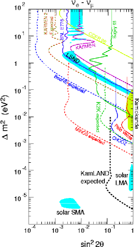
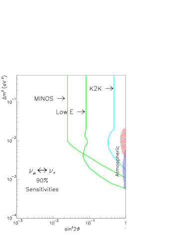
Figure 20: Left panel: results of the present and sensitivities of future $\nu_{e}\leftrightarrow\nu_{\mu}$ oscillations searches (90% c.l.) [67]. Right panel: sensitivities of MINOS and K2K long baseline experiments [68].

In the 3-flavour framework, the oscillations due to the large $\Delta m_{atm}^{2}\sim 3\times 10^{-3}$ eV² should be in the averaging regime in the KamLAND experiment and therefore the $\bar{\nu}_{e}$ survival probability should be described by eqs. (74) and (75) rather than by (72). In the case of SMA, LMA and VO solutions of the solar neutrino problem the $\bar{\nu}_{e}$ survival probability at KamLAND is then just $P(\bar{\nu}_{e}\to\bar{\nu}_{e})\simeq c_{13}^{4}$, i.e. the mixing angle $\theta_{13}$ is directly measured. The CHOOZ data allow $c_{13}^{4}\buildrel>\over{{}_{\sim}}0.90$ for $\Delta m_{atm}^{2}$ in the SK range. In the case of the LMA solution, $P(\bar{\nu}_{e}\to\bar{\nu}_{e})_{\small 3fl}\simeq c_{13}^{4}P(\bar{\nu}_{e}\to\bar{\nu}_{e})_{\small 2fl}$ where $P(\bar{\nu}_{e}\to\bar{\nu}_{e})_{\small 2fl}$ is the usual 2-flavour survival probability (75). Thus, in this case the 2-flavour analysis is modified by a non-vanishing $\theta_{13}$.

There have been a number of accelerator experiments looking for neutrino oscillations. In all but one no evidence for oscillations was found and constraints on oscillation parameters were obtained [65, 68]. The LSND Collaboration have obtained an evidence for $\bar{\nu}_{\mu}\to\bar{\nu}_{e}$ and $\nu_{\mu}\to\nu_{e}$ oscillations [4]. The LSND result is the only indication for neutrino oscillations that is a signal and not a deficiency. The KARMEN experiment is looking for neutrino oscillations in $\bar{\nu}_{\mu}\to\bar{\nu}_{e}$ channel. No evidence for oscillations has been obtained, and part of the LSND allowed region has been excluded. In fig. 19 (right panel) the results from LSND and KARMEN experiments are shown along with the relevant constraints from the BNL776 and Bugey experiments. One can see that the only domain of the LSND allowed region which is presently not excluded is a narrow strip with $\sin^{2}2\theta\simeq 1.5\times 10^{-3}-4\times 10^{-2}$ and $\Delta m^{2}\simeq 0.2-2$ eV².

The existing neutrino anomalies (solar neutrino problem, atmospheric neutrino anomaly and the LSND result), if all interpreted in terms of neutrino oscillations, require three different scales of mass squared differences: $\Delta m^{2}_{\odot}\buildrel<\over{{}_{\sim}}10^{-4}$ eV², $\Delta m^{2}_{atm}\sim 10^{-3}$ eV² and $\Delta m^{2}_{\rm LSND}\buildrel>\over{{}_{\sim}}0.2$ eV². This is only possible with four (or more) light neutrino species. The fourth light neutrino cannot be just the 4th generation neutrino similar to $\nu_{e}$, $\nu_{\mu}$ and $\nu_{\tau}$ because this would be in conflict with the experimentally measured width of $Z^{0}$ boson [see eq. (2)]. It can only be an electroweak singlet (sterile) neutrino. Therefore the LSND result, if correct, would imply the existence of a light sterile neutrino.

Out of all experimental evidences for neutrino oscillations, the LSND result is the only one that has not yet been confirmed by other experiments. It is therefore very important to have it independently checked. This will be done by the MiniBooNE (first phase of BooNE) experiment at Fermilab. MiniBooNE will be capable of observing both $\nu_{\mu}\to\nu_{e}$ appearance and $\nu_{\mu}$ disappearance. If the LSND signal is due to $\nu_{\mu}\to\nu_{e}$ oscillations, MiniBooNE is expected to detect an excess of $\sim$1500 $\nu_{e}$ events during its first year of operation, establishing the oscillation signal at $\sim 8\sigma$ level (see fig. 20). If this happens, the second detector will be installed, with the goal to accurately measure the oscillation parameters. MiniBooNE will begin taking data in 2002.

A number of long baseline accelerator neutrino experiments have been proposed to date. They are designed to independently test the oscillation interpretation of the results of the atmospheric neutrino experiments, accurately measure the oscillation parameters and to (possibly) identify the oscillation channel. The first of these experiments, K2K (KEK to Super-Kamiokande) already started taking data in 1999. It has a baseline of 250 km and is looking for $\nu_{\mu}$ disappearance. K2K should be able to test practically the whole region of oscillation parameters allowed by the SK atmospheric neutrino data except perhaps the lowest-$\Delta m^{2}$ part of it (see fig. 20). Two other long baseline projects, NuMI - MINOS (Fermilab to Soudan mine in the US) and CNGS (CERN to Gran Sasso in Europe), each with the baseline of about 730 km, will be sensitive to smaller values of $\Delta m^{2}$ and should be able to test the whole allowed region of SK (fig. 20). MINOS will look for $\nu_{\mu}$ disappearance and spectrum distortions due to $\nu_{\mu}\to\nu_{x}$ oscillations. It may run in three different energy regimes – high, medium and low energy. MINOS is scheduled to start data taking in the end of 2002. CERN to Gran Sasso will be an appearance experiment looking specifically for $\nu_{\mu}\to\nu_{\tau}$ oscillations. It will also probe $\nu_{\mu}\to\nu_{e}$ appearance. At the moment, two detectors have been approved for participation in the experiment – OPERA and ICANOE. The whole project was approved in December of 1999 and the data taking is planned to begin on May 15, 2005 [5].

Among widely discussed now future projects are neutrino factories – muon storage rings producing intense beams of high energy neutrinos. In addition to high statistics studies of neutrino interactions, experiments at neutrino factories should be capable of measuring neutrino oscillation parameters with high precision and probing the subdominant neutrino oscillation channels, matter effects and CP violation effects in neutrino oscillations [69].

13 Phenomenological neutrino mass matrices

The information on neutrino masses and lepton mixing obtained in solar and atmospheric the neutrino experiments can be summarized as follows:

$${\rm SMA:}\quad\quad \Delta m_{\odot}^{2}\simeq(4-10)\cdot 10^{-6}~{}{\rm eV}^{2}\,,\quad\quad \sin^{2}2\theta_{\odot}\simeq(0.1-1.0)\cdot 10^{-2}$$

$${\rm LMA:}\quad\quad \Delta m_{\odot}^{2}\simeq(2-20)\cdot 10^{-5}~{}{\rm eV}^{2}\,,\quad\quad \sin^{2}2\theta_{\odot}\simeq 0.65-0.97$$

$${\rm VO:}\quad\quad ~{}~{}\Delta m_{\odot}^{2}\simeq(0.5-5)\cdot 10^{-10}~{}{\rm eV}^{2}\,,\quad\quad \sin^{2}2\theta_{\odot}\simeq 0.6-1.0$$

$${\rm Atm:}\quad\quad ~{}\Delta m_{atm}^{2}\simeq(2-6)\cdot 10^{-3}~{}{\rm eV}^{2}\,,\quad\quad \sin^{2}2\theta_{atm}\simeq 0.82-1.0$$ (143)

In the 3-flavour framework (neglecting the LSND result), $\Delta m_{\odot}$ has to be identified with $\Delta m_{21}^{2}$, $\Delta m_{atm}$ with $\Delta m_{31}^{2}\simeq\Delta m_{32}^{2}$, $\theta_{\odot}$ with $\theta_{12}$, and $\theta_{atm}$ with $\theta_{23}$. The 2-flavour analysis gives a good first approximation to the results of the 3-flavour studies [53, 57] because the mixing angle $\theta_{13}$ is constrained to be rather small by the CHOOZ data (142).

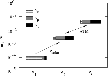
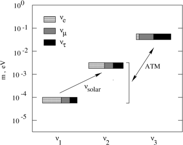
Figure 21: 3-flavour schemes of neutrino masses and mixing. Solutions of the solar neutrino problem are SMA (left panel) and LMA right panel) [70]

A very concise and illuminating way of summarizing the neutrino data is to present the neutrino mass eigenstates graphically as rectangles of unit area, the position of which on the vertical scale reflects their mass whereas the areas of differently marked parts are equal to $|U_{ai}|^{2}$, i.e. to the weights with which the $a$th flavor eigenstate is present in the $i$th mass eigenstate [70]. In the 3-flavour framework, the present-day data allow three main possibilities corresponding to the three main solutions of the solar neutrino problem. They are shown in fig. 21 and in fig. 22 (left panel). The schemes have different contributions of $\nu_{e}$, $\nu_{\mu}$ and $\nu_{\tau}$ in the two low-lying mass eigenstates. The weight of $\nu_{e}$ in the mass eigenstate $\nu_{3}$ which is separated from $\nu_{1}$ and $\nu_{2}$ by a large mass gap is $|U_{e3}|^{2}$; it is either small or zero. The weights of $\nu_{\mu}$ and $\nu_{\tau}$ within each mass eigenstate are approximately equal to each other as a consequence of $\theta_{23}\simeq 45^{\circ}$ and $|U_{e3}|^{2}=s_{13}^{2}\ll 1$. This, in particular, means that the solar neutrinos oscillate into an almost equal superposition of $\nu_{\mu}$ and $\nu_{\tau}$, independently of the type of the solution of the solar neutrino problem (SMA, LMA, LOW or VO). The scheme of the left panel of fig. 21 corresponds to single large mixing, whereas those of the right panel of fig. 21 and left panel of fig. 22 describe bi-large or bi-maximal (in the case $U_{e3}=0$) mixing. The 3-flavour schemes of figs 21 and 22 correspond to the so-called normal neutrino mass hierarchy, $m_{1}\ll m_{2}\ll m_{3}$. In addition, there are schemes (not shown in the figures) in which the position of the mass eigenstate $\nu_{3}$ and of the pair ($\nu_{1},\nu_{2}$) are interchanged (inverted mass hierarchy, $m_{3}\ll m_{1}\simeq m_{2}$). The present-day data do not discriminate between the normal and inverted hierarchies; such a discrimination may become possible in future if the earth’s matter effects in atmospheric or long baseline $\nu_{e}\leftrightarrow\nu_{\mu}$ or $\nu_{e}\leftrightarrow\nu_{\tau}$ oscillations are observed.

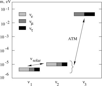
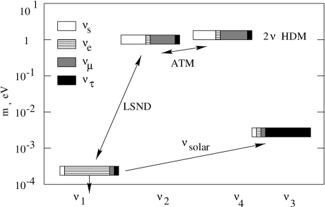
Figure 22: Schemes of neutrino masses and mixing. Left panel: 3-flavour scheme with the VO solution of the solar neutrino problem. Right panel: SMA solution in the 4-flavour scheme [70].

The normal and inverted neutrino mass hierarchies discussed above do not exhaust all possible schemes of 3-flavour neutrino mass schemes. Since neutrino oscillation experiments only allow the determination of neutrino mass squared differences and not of the masses themselves, it is also possible that neutrinos are quasi-degenerate in mass, and only their mass squared differences satisfy the hierarchies shown in figs. 21 and 22. Direct neutrino mass measurements allow the average neutrino mass as large as a few eV (provided that the $2\beta 0\nu$ constraint (127) is satisfied). In that case neutrinos could constitute a significant fraction of the dark matter of the universe (hot dark matter).

If the LSND result is correct, there should be at least four light neutrino species. Four-flavour neutrino schemes can be analyzed similarly to the 3-flavour case. The data allow essentially two schemes. In each of these schemes there are two pairs of nearly degenerate mass eigenstates separated by large $\Delta m_{LSND}^{2}$. The mass splittings between the components of the quasi-degenerate pairs are $\Delta m_{\odot}^{2}$ and $\Delta m_{atm}^{2}$. An example of a 4-flavour scheme is shown in fig. 22 (right panel). More detailed discussions of the 4-flavour schemes can be found in [71].

Table 2: Zeroth order form of the neutrino mass matrix for double and single maximal mixing. A  – normal mass hierarchy, B – inverted hierarchy, C – quasi-degenerate neutrinos. From [72].

		double	single
	$m_{diag}$	maximal	maximal
		mixing	mixing
A	Diag[0,0,1]	$\left[\matrix{0&0&0\cr 0&1/2&-1/2\cr 0&-1/2&1/2}\right]$	$\left[\matrix{0&0&0\cr 0&1/2&-1/2\cr 0&-1/2&1/2}\right]$
B1	Diag[1,-1,0]	$\left[\matrix{0&1/\sqrt{2}&1/\sqrt{2}\cr 1/\sqrt{2}&0&0\cr 1/\sqrt{2}&0&0}\right]$	$\left[\matrix{1&0&0\cr 0&-1/2&-1/2\cr 0&-1/2&-1/2}\right]$
B2	Diag[1,1,0]	$\left[\matrix{1&0&0\cr 0&1/2&1/2\cr 0&1/2&1/2}\right]$	$\left[\matrix{1&0&0\cr 0&1/2&1/2\cr 0&1/2&1/2}\right]$
C0	Diag[1,1,1]	$\left[\matrix{1&0&0\cr 0&1&0\cr 0&0&1}\right]$	$\left[\matrix{1&0&0\cr 0&1&0\cr 0&0&1}\right]$
C1	Diag[-1,1,1]	$\left[\matrix{0&-1/\sqrt{2}&-1/\sqrt{2}\cr-1/\sqrt{2}&1/2&-1/2\cr-1/\sqrt{2}&-1/2&1/2}\right]$	$\left[\matrix{-1&0&0\cr 0&1&0\cr 0&0&1}\right]$
C2	Diag[1,-1,1]	$\left[\matrix{0&1/\sqrt{2}&1/\sqrt{2}\cr 1/\sqrt{2}&1/2&-1/2\cr 1/\sqrt{2}&-1/2&1/2}\right]$	$\left[\matrix{1&0&0\cr 0&0&-1\cr 0&-1&0}\right]$
C3	Diag[1,1,-1]	$\left[\matrix{1&0&0\cr 0&0&1\cr 0&1&0}\right]$	$\left[\matrix{1&0&0\cr 0&0&1\cr 0&1&0}\right]$

The experimental information on the neutrino masses and lepton mixing angles allows one to reconstruct the phenomenologically allowed forms of the neutrino mass matrix. This can be done by inverting the relation $(m_{L})_{diag}=diag(m_{1},\,m_{2},\,m_{3})=U^{T}m_{L}\,U$. The detailed structure of the neutrino mass matrix $m_{L}$ is not yet known since some of the neutrino parameters are still rather uncertain. However, one can derive the zeroth-approximation structures (textures) of the neutrino mass matrices just using the already known gross features of neutrino spectrum and mixing angles. In particular, in the zeroth approximation one can assume $m_{1}=m_{2}$, $s_{13}=0$, $\theta_{23}=45^{\circ}$. Some of the neutrino mass matrix textures that can be obtained in this way are summarized in Table 2 taken from [72]. Notice that these textures are defined only up to the trivial sign changes due to the rephasing of the neutrino fields.

In realistic models, zeros in neutrino mass textures must be filled with small elements and in addition the large entries can be perturbed by small corrections. The small entries of the neutrino mass matrices should satisfy certain constraints; one of them follows from the requirement that for the LMA and SMA MSW solutions of the solar neutrino problem the lower-lying of the mass eigenstates $\nu_{1}$ and $\nu_{2}$ have a larger $\nu_{e}$ component. As was discussed in sec. 8, if this condition is not satisfied, the MSW resonance is only possible for antineutrinos and not for neutrinos. This requirement on the small entries of the neutrino mass matrices disfavours the inverted mass hierarchy and quasi-degenerate neutrinos and favours the normal mass hierarchy [73].

The neutrino mass matrix textures can provide us with a hint of the symmetries or dynamics underlying the theory of neutrino mass. With the forthcoming data from future neutrino experiments, it may eventually become possible to unravel the mechanism of the neutrino mass generation, which may hold the clue to the general fermion mass problem.

We live in a very fascinating time for neutrino physics. It is very likely that in a few years from now new solar and long baseline neutrino experiments will bring us an important knowledge about neutrinos allowing to answer many questions and solving the solar neutrino problem. Neutrinos may also bring us new surprises, as they did many times in the past.

References

- [1] Super-Kamiokande Collaboration, Y. Fukuda et al., Phys. Rev. Lett. 81 (1998) 1562; ibid. 82 (1999) 2644; ibid. 82 (1999) 5194; hep-ex/9908049.
- [2] For a recent review see, e.g., Y. Suzuki, Talk at the XIX International Symposium on Lepton and Photon Intaractions at High Energies, Stanford University, August 914, 1999.
- [3] For a recent review see, e.g., W.A. Mann, Talk at the XIX International Symposium on Lepton and Photon Intaractions at High Energies, Stanford University, August 914, 1999; hep-ex/9912007.
- [4] LSND Collaboration, C. Athanassopoulos et al., Phys. Rev. Lett. 81 (1998) 1774; Phys. Rev. C 58 (1998) 2489.
- [5] For numerous links to various solar, atmospheric, reactor, accelerator and other neutrino experiments see the Neutrino Oscillation Industry Web page maintained by M. Goodman, http://www.hep.anl.gov/ndk/hypertext/nu_industry.html
- [6] L. Wolfenstein, Phys. Rev. D17 (1978) 2369; S.P. Mikheyev, A. Yu. Smirnov, Sov. J. Nucl. Phys. 42 (1985) 913.
- [7] For history of neutrino physics see, e.g., P. Ramond, hep-ph/9809401; S.M. Bilenky, hep-ph/9710251, hep-ph/9908335; W.C. Haxton, B.R. Holstein, hep-ph/9905257; M. Nakagawa, hep-ph/9902413.
- [8] K.S. Babu, lectures at this school, to be published in the Proceedings.
- [9] A.Yu. Smirnov, hep-ph/9901208; R.N. Mohapatra, hep-ph/9910365; J.W.F. Valle, hep-ph/9907222.
- [10] T.P. Walker, lectures at this school, to be published in the Proceedings.
- [11] G.G. Raffelt, Stars as Laboratories for Fundamental Physics, Chicago Univ. Press, 1996; hep-ph/9902271; hep-ph/9903472.
- [12] S. Sarkar, Rep. Prog. Phys.59 (1996) 1493; hep-ph/9602260.
- [13] G.G. Raffelt, W. Rodejohann, Lectures given at 4th National Summer School for German-speaking Graduate Students of Theoretical Physics, Saalburg, Germany, 31 Aug - 11 Sep 1998, hep-ph/9912397.
- [14] S.M. Bilenky, S.T. Petcov, Rev. Mod. Phys. 59 (1987) 671; Erratum: ibid. 61 (1989) 169.
- [15] P.B. Pal, R.N. Mohapatra, Massive Neutrinos in Physics and Astrophysics, World Scientific, Singapore, 1991.
- [16] E.Kh. Akhmedov, hep-ph/9705451; J. Pulido, Phys. Rep. 211 (1992) 167.
- [17] G. Gelmini, E. Roulet, Rep. Prog. Phys. 58 (1995) 1207, hep-ph/9412278.
- [18] S.M. Bilenky, C. Giunti, W. Grimus, Prog. Part. Nucl. Phys. 43 (1999) 1.
- [19] C.W. Kim, A. Pevsner, Neutrinos in Physics and Astrophysics, Harwood Academic, 1993.
- [20] F. Boehm, P. Vogel, Physics of Massive Neutrinos, Cambridge Univ. Press, 1992.
- [21] Particle Data Group, C. Caso et al., Eur. Phys. J. C3 (1998) 1.
- [22] B. Kayser, Phys. Rev. D30 (1984) 1023.
- [23] V.A. Rubakov, M.E. Shaposhnikov, Phys. Usp. 39 (1996) 461; hep-ph/9603208.
- [24] S. Weinberg, Phys. Rev. Lett. 43 (1979) 1566; R. Barbieri, J. Ellis, M.K. Gaillard, Phys. Lett. B90 (1980) 249; E. Akhmedov, Z. Berezhiani, G. Senjanovic, Phys. Rev. Lett. 69 (1992) 3013.
- [25] G.B. Gelmini, M. Roncadelli, Phys. Lett. B99 (1981) 411.
- [26] J.C. Pati, A. Salam, Phys. Rev. D10 (1974) 275; R.N. Mohapatra, J.C. Pati, Phys. Rev. D11 (1975) 2558; G. Senjanović, R.N. Mohapatra, Phys. Rev. D12 (1975) 1502.
- [27] M. Gell-Mann, P. Ramond and R. Slansky, in Supergravity, ed. by P. van Nieuwenhuizen and D. Z. Freedman (North Holland, Amsterdam, 1979), p. 315; T. Yanagida, in Proc. of the Workshop on the Unified Theory and Baryon Number in the Universe, ed. by O. Sawada and A. Sugamoto (KEK report 79-18, 1979), p.95, Tsukuba, Japan; R.N. Mohapatra and G. Senjanović, Phys. Rev. Lett. 44 (1980) 912.
- [28] B. Pontecorvo, Sov. Phys. JETP 6 (1958) 429; Sov. Phys. JETP 7 (1958) 172.
- [29] Z. Maki, M. Nakagawa, S. Sakata, Progr. Theor. Phys. 28 (1962) 870.
- [30] S.P. Mikheyev, A.Yu. Smirnov, Sov. Phys. Usp. 30 (1987) 759; Prog. Part. Nucl. Phys. 23 (1989) 41.
- [31] A.Yu. Smirnov, G.T. Zatsepin, Mod. Phys. Lett. A7 (1992) 1272.
- [32] S.M. Bilenky, J. Hošek, S.T. Petcov, Phys. Lett. B94 (1989) 495; I.Yu. Kobzarev et al., Sov. J. Nucl. Phys. 32 (1980) 823; M. Doi it et al., Phys. Lett. B102 (1981) 323; P. Langacker et al., Nucl. Phys. B282 (1987) 589.
- [33] For reviews see, e.g., [30, 18] and T.K. Kuo, J. Pantaleone, Rev. Mod. Phys. 61 (1989) 937.
- [34] C. Lunardini, A.Yu. Smirnov, in preparation.
- [35] C. Giunti, C.W. Kim, M. Monteno, Nucl. Phys. B521 (1998) 3.
- [36] E.Kh. Akhmedov, Nucl. Phys. B538 (1999) 25.
- [37] E.Kh. Akhmedov et al., Nucl. Phys. B542 (1999) 3.
- [38] C.-S. Lim, preprint BNL-39675, 1987.
- [39] For recent discussion of CP violation in neutrino oscillations see, e.g., A. De Rújula, M. B. Gavela and P. Hernández, Nucl. Phys. B547 (1999) 21; K. Dick et al., Nucl. Phys. B562 (1999) 29-56; M. Tanimoto, Phys. Lett. B462 (1999) 115; A. Donini et al., hep-ph/9909254; M. Koike, J. Sato, hep-ph/9909469.
- [40] Z.G. Berezhiani, M.I. Vysotsky, Phys. Lett. B199 (1987) 281; Z.G. Berezhiani, A.Yu. Smirnov, Phys. Lett. B220 (1989) 279.
- [41] L.B. Okun, M.B. Voloshin, M.I. Vysotsky, Sov. Phys. JETP 64 (1986) 446, Erratum: ibid. 65 (1987) 209; C.-S. Lim, W.J. Marciano, Phys. Rev. D37 (1988) 1368; E.Kh. Akhmedov, Phys. Lett. B213 (1988) 64.
- [42] V.K. Ermilova, V.A. Tsarev, V.A. Chechin, Short Notices of the Lebedev Institute 5 (1986) 26.
- [43] E. Kh. Akhmedov, Yad. Fiz. 47 (1988) 475.
- [44] Q.Y. Liu, A. Yu. Smirnov, Nucl. Phys. B524 (1998) 505; Q.Y. Liu, S.P. Mikheyev, A. Yu. Smirnov, Phys. Lett. B440 (1998) 319.
- [45] S.T. Petcov, Phys. Lett. B434 (1998) 321.
- [46] Heidelberg-Moscow Collaboration, L. Baudis et al., Phys. Rev. Lett. 83 (1999) 41; H.V. Klapdor-Kleingrothaus, Int. J. Mod. Phys. 13 (1998) 3953.
- [47] J. Schechter, J.W.F. Valle, Phys. Rev. D25 (1982) 2951.
- [48] J.N. Bahcall’s home page, http://www.sns.ias.edu/jnb/
- [49] J.N. Bahcall, astro-ph/9808162.
- [50] J.N. Bahcall, P.I. Krastev, A.Yu. Smirnov, Phys. Rev. D58 (1998) 096016.
- [51] M. C. Gonzalez-Garcia, P. C. de Holanda, C. Peña-Garay, J. W. F. Valle, hep-ph/9906469.
- [52] Y. Totsuka, Invited talk given at the XV Int. Conf. Particle and Nuclei (PANIC99), Uppsala, Sweden, June 10-19, 1999.
- [53] G. Fogli et al., hep-ph/9912231; M.C. Gonzalez-Garcia, C. Peña-Garay, hep-ph/0001129.
- [54] S.P. Mikheyev, A.Yu. Smirnov, Phys. Lett. B429 (1998) 343.
- [55] K. Scholberg, hep-ex/9905016.
- [56] M. Honda et al., Phys. Rev. D52 (1995) 4985.
- [57] G.L. Fogli et al., Phys. Rev. D59 (1999) 033001, hep-ph/9808205; hep-ph/9904465.
- [58] O.L.G. Peres, A.Yu. Smirnov, Phys. Lett. B456 (1999) 204.
- [59] M.C. Gonzalez-Garcia et al., Phys. Rev. Lett. 82 (1999) 3202.
- [60] S. Coleman, S.L. Glashow, Phys. Lett. B405 (1997) 249; S.L. Glashow et al., Phys. Rev. D56 (1997) 2433; S. Coleman and S.L. Glashow, Phys. Rev. D59 (1999) 116008; M. Gasperini, Phys. Rev. D38 (1988) 2635; Phys. Rev. D39 (1989) 3606.
- [61] V. Barger et al., Phys. Rev. Lett. 82 (1999) 2640.
- [62] G.L. Fogli et al., Phys.Rev. D60 (1999) 053006.
- [63] V. Barger et al., Phys. Lett. B462 (1999) 109.
- [64] G. Gratta, hep-ex/9905011.
- [65] L. DiLella, hep-ex/9912010.
- [66] CHOOZ Collaboration, M. Apollonio et al., hep-ex/9907037.
- [67] A. Suzuki, Talk given at 8th International Workshop on Neutrino Telescopes, Venice, Italy, February 23 - 26, 1999.
- [68] J. Conrad, hep-ex/9811009.
- [69] For discussions of neutrino oscillation experiments at muon storage rings see, e.g., A. De Rújula, M. B. Gavela and P. Hernández, ref. [39]; M. Campanelli, A. Bueno and A. Rubbia, hep-ph/9905240; V. Barger, S. Geer and K. Whisnant, hep-ph/9906487; O. Yasuda, hep-ph/9910428; I. Mocioiu and R. Shrock, hep-ph/9910554; V. Barger, S. Geer, R. Raja and K. Whisnant, hep-ph/9911524. M. Freund et al., hep-ph/9912457.
- [70] A.Yu. Smirnov, Invited talk at 34th Rencontres de Moriond: Electroweak Interactions and Unified Theories, Les Arcs, France, March 13-20, 1999; hep-ph/9907296.
- [71] For recent discussions of neutrino mass and mixing schemes and data analyses in the 4-flavour framework, see e.g. C. Giunti, hep-ph/9909395; D. Dooling et al., hep-ph/9908513; C. Giunti, M.C. Gonzalez-Garcia, C. Peña-Garay, hep-ph/0001101.
- [72] G. Altarelli, F. Feruglio, hep-ph/9905536.
- [73] E.Kh. Akhmedov, Phys. Lett. B467 (1999) 95.