TAUP 2616-99
BNL - NT-99/11

A Pomeron Approach to Hadron-Nucleus and Nucleus-Nucleus “Soft” Interactions at High Energy

Abstract

We formulate a generalization of the Glauber formalism for hadron-nucleus and nucleus-nucleus collisions based on the Pomeron approach to high energy interactions. Our treatment is based on two physical assumptions ( i.e. two small parameters ) : (i) that only sufficiently small distances contribute to the Pomeron structure; and (ii) the triple Pomeron vertex $G_{3P}/g_{P-N}\,\ll\,1$ (where $g_{P-N}$ is the Pomeron-nucleon vertex) is small. A systematic method is developed for calculating the total, elastic and diffractive dissociation cross sections as well as the survival probability of large rapidity gap processes and inclusive observables, both for hadron - nucleus and nucleus-nucleus collisions. Our approach suggests saturation of the density of the produced hadrons in nucleus-nucleus collisions, the value of the saturation density turns out to be large and depends on the number of nucleons in the lightest nucleus.

1 Introduction

Although QCD is believed to be the microscopic theory of strong interactions it has led to little progress in the theoretical understanding of ”soft” interactions at high energies. At present we only have a phenomenological description of such processes where the main postulate of this description is the Pomeron - a Reggeon with a trajectory intercept $\alpha_{P}(0)$ close to unity,

$$\alpha_{P}(t)\,=\,\alpha_{P}(0)\,+\,\alpha^{\prime}_{P}(0)|t|\,\,;\,\,\,\,\,\,\,\alpha_{P}(0)=1+\Delta,\,\,;\,\,\,\,\,\,\Delta\,\,\ll\,\,1\,\,.$$ (1.1)

We have two comments on the Pomeron hypothesis:

1. The first one is negative. There is a paucity of ideas and/or examples of how a Reggeon such as the Pomeron can be justified theoretically. As far as we know, the only theoretical model, where the Pomeron appears naturally, is a 2 + 1 dimensional QCD [1] which can hardly be considered as a good approximation to reality. The entity closest to the Pomeron, which follows from perturbative QCD (pQCD) is the BFKL Pomeron [2]. In the following, when dealing with ”soft” interactions, we shall also refer to the BFKL Pomeron, but only with regard to the general structure of pQCD approach at high energy.

2. The second comment is positive. In spite of all theoretical uncertainties the Pomeron has been at the heart of high energy phenomenology over the past three decades, providing a good description of all available experimental data [4],[5], [6]. Consequently, we cannot ignore the Pomeron hypothesis as well as the numerous attempts to find a selfconsistent approach based on this postulate.

Even if we accept the Pomeron hypothesis, there still remains a lot of hard work to find the high energy scattering amplitude that includes the Pomeron exchanges, as well as the interactions between

Pomerons. The goal of this paper is to find a solution to this problem for hadron-nucleus and nucleus-nucleus high energy collisions. Our approach is based on two main ideas: (i) a new sufficiently hard scale for the Pomeron structure and (ii) a specific parameter ($\kappa_{A}$) for the Pomeron interaction with a nucleus suggested by Schwimmer [7] many years ago,

$$\kappa_{A}\,\,=\,\,A\,\cdot\,\frac{g_{PN}\,G_{3P}}{\pi R^{2}_{A}}\,\,\cdot\,\,\frac{1}{\Delta}\{\,(\,\frac{s}{s_{0}}\,)^{\Delta}\,\,-\,\,1\,\}\,\,,$$ (1.2)

where $g_{PN}$ is the Pomeron-nucleon vertex, $G_{3P}$ is the triple Pomeron vertex and $\Delta$ is defined in Eq. (1.1). $A$ and $R_{A}$ are the atomic number and the radius of a nucleus, which are defined by

$$R_{A}=A^{\frac{2}{3}}\cdot 17GeV^{-2}.$$ (1.3)

1.1 A new scale for the Pomeron structure

Our key assumption is a new scale for the Pomeron structure, i.e. a sufficiently large mean transverse momentum of partons in the Pomeron ( $<p_{t}>\,\geq\,1\,GeV$ ). We list, first, the experimental and phenomenological observations that support our point of view (see also Ref.[8]):

1. Experimental elasting scattering data can be fitted using a very small value for the slope of the Pomeron trajectory ( see Refs. [4],  [5],  [6], [9] ): $\alpha_{P}^{\prime}=0.25GeV^{-2}\,\ll\,\alpha_{R}^{\prime}=1GeV^{-2}$, here $\alpha_{R}^{\prime}$ is the slope of the Reggeon trajectory ( see Eq. (1.1) );

2. The experimental $\frac{d\sigma}{dt}$ slope of single diffraction dissociation, with final state secondary hadron system with a large mass, is approximately two times smaller than the slope for the elastic scattering. The description of the diffractive dissociation processes is closely connected to the triple Pomeron vertex, $G_{3P}$ ( see Fig. 1 ). A small slope leads to a small proper size of this vertex. As a first approximation we can assign a zero slope to the triple Pomeron vertex, as this provides a reasonable description of the experimental single diffractive dissociation data.

   

   Figure 1: $G_{3P}$ and the diffractive dissociation process.

3. The HERA data [10] on diffractive photoproduction of J/$\Psi$ and deep inelastic scattering ( DIS), show that the $t$- slope for elastic diffractive dissociation ( $\gamma^{*}+p\,\,\rightarrow\,\,J/\Psi+p$ ) is larger than the $t$-slope for the inelastic channel ( $\gamma^{*}+p\,\,\rightarrow\,\,J/\Psi+N^{*}$, where $N^{*}$ is the nucleon exitation ). These data provide direct experimental support for the idea that there are two typical scales for the size inside a hadron, namely, the distance between quarks and the proper size of the constituent quarks in the Additive Quark Model( AQM )[11]. In the AQM the size of the constituent quark is closely related to the typical transverse momentum of partons in the Pomeron.

4. The main idea of the AQM that gluons inside a hadron are confined in a volume of a smaller radius ( $R_{G}\,\approx\,0.1fm\,\ll\,R_{h}\,\approx\,1\,fm$ ), is a working hypothesis which is included in the standard Pomeron phenomenology that describes the experimental data [4].

5. The HERA experimental data [9] have confirmed the theoretical expectation [12] that the density of partons in a hadron at low $x$ reaches a high value. In high density QCD we expect that a new saturation scale appears [12]. This saturation scale means that the average transverse momentum of a parton becomes large in the region of high density and, therefore, it confirms our assumption regarding a new scale associated with the Pomeron.

The consequence of assuming a new hard scale in the Pomeron leads to:

• The Pomeron exchange as well as all vertices for the Pomeron-Pomeron interaction, can be viewed as delta functions in impact parameter ( $b_{t}$ ) representation. Indeed, based on our assumption, we can neglect both $\alpha^{\prime}_{P}(0)$ and the proper size of all Pomeron-Pomeron vertices, and consider the Green’s function for the Pomeron exchange, as well as the vertices, as constants in momentum representation, or in other words, as delta functions in $b_{t}$-representation:

  $$P(s,b_{t})\,\,=\,\,i\,\,\delta^{(2)}(\vec{b}_{t})\,(\,\frac{s}{s_{0}}\,)^{\Delta}\,\,;$$ (1.4)

  $$G_{3P}(b_{t})\,\,=\,\,\,G_{3P}(0)\,\delta^{(2)}(\vec{b}_{t})\,\,;\,\,\,\,\,\,G_{4P}(b_{t})\,\,=\,\,\,G_{4P}(0)\,\delta^{(2)}(\vec{b}_{t})$$ . (1.5)

  Consequently, in our approach, all the $b_{t}$ dependence is concentrated in the Pomeron - hadron vertices which depend on the size of a hadron. We use the simplest Gaussian parametrization for the Pomeron-Nucleus vertex, i.e.:

  $$g_{PA}(b_{t})\,\,\,=\,\,\,A\,\frac{g_{PN}}{\pi R^{2}_{A}}\,\,\exp\left(-\frac{b^{2}_{t}}{R^{2}_{A}}\right)\,\,,$$ (1.6)

  where the notation is the same as in Eq. (1.2). Combining Eq. (1.6) with Eq. (1.4) one can obtain that for nucleus ($A_{1}$) - nucleus ($A_{2}$) scattering, the single Pomeron exchange has the form ( at fixed $b_{t}$ ):

  $$\int\,\,d^{2}\,b^{\prime}_{t}\,\,\int\,d^{2}\,b"_{t}\,g_{PA_{1}}(b^{\prime}_{t})\,\,P(s,{\vec{b^{\prime}}}_{t}-{\vec{b"}}_{t})\,\,g_{PA_{2}}({\vec{b}}_{t}-{\vec{b"}}_{t})\,\,=$$ (1.7)

  $$\,\,\frac{g^{2}_{PN}\,\cdot A_{1}\,\cdot\,A_{2}}{\pi R^{2}_{A_{1}}\,\cdot\,\pi R^{2}_{A_{2}}}\,\,\cdot\,\,\int\,d^{2}\,b^{\prime}_{t}\,\,\exp\left(-\frac{b^{\prime 2}_{t}}{R^{2}_{A_{1}}}\right)\,\cdot\,\left(\,\frac{s}{s_{0}}\,\right)^{\Delta}\,\cdot\,\exp\left(-\frac{({\vec{b}}_{t}-{\vec{b^{\prime}}}_{t})^{2}}{R^{2}_{A_{2}}}\right)\,\,$$

  $$=\,\,\frac{g^{2}_{PN}\,\cdot A_{1}\,\cdot\,A_{2}}{\pi(R^{2}_{A_{1}}\,+\,R^{2}_{A_{2}})}\,\cdot\,\left(\,\frac{s}{s_{0}}\,\right)^{\Delta}\,\cdot\,\exp\left(-\frac{b^{2}_{t}}{R^{2}_{A_{1}}\,+\,R^{2}_{A_{2}}}\right)\,\,.$$

• We can use pQCD to estimate the values for the vertices of the Pomeron-Pomeron interactions, since the typical scale ( the Pomeron radius ) is small. Simply counting the number of $\alpha_{S}$ in the pQCD diagrams gives ( see Refs. [2] [8] [12] [14] )

  $$g_{PN}\,\,\propto\,\,\,\alpha_{S}\,\,;\,\,\,\,\,\,\,\,\,\Delta\,\,\,\propto\,\,\,\alpha_{S}N_{c}\,\,;$$ (1.8)

  $$G_{3P}\,\,\,\propto\,\,\,\alpha_{S}^{2}N_{c}\,\,;\,\,\,\,\,\,\,\,\,G_{4p}\,\,\,\,\propto\,\,\,\alpha_{S}^{2}\,\,.$$ (1.9)

  To select the vertices of the Pomeron-Pomeron interaction we use the main principle of the large $N_{c}$ ( number of colours ) approximation, that has been formulated by Veneziano et al. [15]. We sum separately in each topological configuration the leading $N_{c}$ diagrams, considering $N_{c}\alpha_{S}\,\,\approx\,1$, while $\alpha_{S}\,\,\ll\,\,1$. Applying these rules to Eq. (1.8) and Eq. (1.9) we see that we can take into account only the triple Pomeron interaction and neglect more complicated vertices.

1.2 The order parameter $\mathbf{\kappa_{A}}$

The problem of summing all triple Pomeron interactions looks hopeless without an additional small parameter that aids us in classifying the numerous Reggeon diagrams, which describe Pomeron interactions ( see Ref, [16] for details ). Such a parameter is $\kappa_{A}$ given by Eq. (1.2) and suggested by Schwimmer[7] more than thirty years ago,

$$\kappa_{A}\,\,=\,\,A\,\cdot\,\frac{g_{PN}\,G_{3P}}{\pi R^{2}_{A}}\,\,\cdot\,\,\frac{1}{\Delta}\{\,(\,\frac{s}{s_{0}}\,)^{\Delta}\,\,-\,\,1\,\}\,\,.$$ (1.10)

To clarify the meaning of $\kappa_{A}$ we calculate the cross section for diffractive dissociation of an incoming hadron in the region of large mass for the hadron-nucleus collision. This process is illustrated in Fig. 1, where the incoming hadron is shown at the bottom of the diagram. Using Eq. (1.4) and Eq. (1.5), the cross section can be written as:

$$\sigma^{SD}(h+A\,\rightarrow\,M+A)\, = \,\int^{Y}_{0}\,dy\,\int\,d^{2}\,b_{t}\,\int\,d^{2}\,b^{\prime}_{t}g^{2}_{PA}(b^{2}_{t})\,g_{PN}((\vec{b}_{t}-\vec{b^{\prime}}_{t})^{2})\,\,G_{3P}\,\,e^{2\,\Delta(Y-y)\,+\,\Delta\,y}\,$$ (1.11)

$$= \,\frac{A^{2}}{\left(\pi R^{2}_{A}\right)^{2}}\,g^{3}_{PN}\,G_{3P}e^{2\,\Delta\,Y}\,\int^{Y}_{0}\,d\,y\,e^{-\,\Delta\,y}\,$$

$$= \,\frac{A\,g^{2}_{PN}}{\pi R^{2}_{A}}\,e^{\Delta\,Y}\cdot\,\frac{A\,g_{PN}\,G_{3P}}{\pi R^{2}_{A}}\,\frac{1}{\Delta}\,\{\,e^{\Delta\,Y}\,\,-\,\,1\,\}$$

$$= \,\frac{A\,g^{2}_{PN}}{\pi R^{2}_{A}}\,e^{\Delta\,Y}\,\cdot\,\kappa_{A}\,\,=\,\,g_{PN}\,g_{PA}\left(b_{t}=0\right)P(Y)\,\cdot\,\kappa_{A}\,\,,$$

where Eq. (1.6) was used and we introduce the notation: $Y=ln(s/s_{0})$, $y=\,ln(M^{2}/s_{0})$ and $P\left(Y\right)=e^{\Delta\,Y}$. From Eq. (1.11) we see that the parameter $\kappa_{A}$ now indicates how large or small the cross section of diffractive dissociation is, in comparison with the total cross section given by Pomeron exchange ( see Eq. (1.7) ). The principle idea of the selection rules for Reggeon diagrams is to sum all diagrams of the order $\kappa^{n}_{A}$, neglecting the diagrams that are proportional to $g^{2n}_{PN}$ or $\kappa^{n}_{N}$. In other words, we consider the following set of parameters:

$$\kappa_{A}\,\,\approx\,\,1\,\,;\,\,\,\,\,\,\,\,\,\,\kappa_{N}\,\,\ll\,\,1\,\,;\,\,\,\,\,\,\,\,\,\,\frac{\gamma}{g_{PN}}\,\cdot\,\kappa_{N}\,\,\ll\,\,1\,\,.$$ (1.12)

Below we show how this set of parameters helps, and the type of selection rules it leads to, both for hadron-nucleus and nucleus-nucleus interaction. Eq. (1.12) only holds for the case of heavy nuclei with $A\,\,\gg\,\,1$. We consider the experimental fact that $G_{3P}/(g_{PN}\cdot\Delta)$ is rather small ($\approx$ 1/4 - 1/8), which follows from measurements of $\sigma_{el}(pp)$ and $\sigma^{SD}(pp)$, as supportive for our approach ( see also section 2.6 for details ).

1.3 The Glauber-Gribov Approach

As we have mentioned, the main goal of this paper is to find a natural generalization of Glauber-Gribov approach[17][18] to hadron - nucleus and nucleus-nucleus interaction at high energies. In this subsection we recall the Glauber-Gribov approach for the nucleus - nucleus interaction (see Fig. 2 ).

Fig. 2-a	Fig. 2-b

Figure 2: Nucleus - Nucleus scattering: The Glauber-Gribov approach (Fig.2-a) and the first corrections (Fig.2-b) to the Glauber-Gribov approach. Figures are taken fron Ref. [18].

Fig. 2-a shows that in the Glauber-Gribov approach we view a nucleus as a collection of almost free nucleons which could interact elastically and/or inelastically with a nucleon in another nucleus. In this approach the

unitarity constraint

$$2\,Im\,a_{el}(s,b_{t})\,\,\,=\,\,|a_{el}(s,b_{t})|^{2}\,\,\,+\,\,\,G_{in}(s,b_{t})\,\,,$$ (1.13)

has a simple solution

$$a_{el}(s,b_{t})\,\, = \,\,i\,\left(\,1\,\,-\,\,\exp\left(-\,\frac{\Omega(s,b_{t})}{2}\right)\,\right)\,\,;$$ (1.14)

$$G_{in}(s,b_{t})\,\, = \,\,1\,\,\,-\,\,\,\exp\left(-\Omega(s,b_{t})\right)\,\,,$$ (1.15)

assuming that the elastic amplitude $a_{el}(s,b_{t})$ is pure imaginary at high energy. In Eq. (1.13) $G_{in}(s,b_{t})$ denotes the contribution of all inelastic processes. The advantages of the Glauber-Gribov approach is that we can express the cross section of a nucleon-nucleon interaction in terms of an arbitrary real function $\Omega(s,b_{t})$, which is known as opacity. Indeed, we can use Eq. (1.7) for rewriting the opacity in in the form:

$$\Omega^{A_{1}-A_{2}}(s,b_{t})\,\,=\,\,A_{1}\times A_{2}\times\sigma^{N-N}_{tot}(s)\int S(|\vec{b}_{t}-\vec{b^{\prime}}_{t})\,\,\cdot\,\,S(b^{\prime}t)\,d^{2}b\,d^{2}b^{\prime}\,,$$ (1.16)

where $\sigma^{N-N}_{tot}(s)$ is the total cross section of the nucleon-nucleon interaction and $S(b_{t})$ is the distribution of nucleons in a nucleus $S(b_{t})=\int dz\rho(z,b_{t})$ where $\rho(z,b_{t})$ is the nucleon density in a nucleus. In Eq. (1.7) we used a Gaussian parametrization for $S(b_{t})$ to simplify our calculations. Formulae given by Eq. (1.14) and Eq. (1.15) with $\Omega$ defined in Eq. (1.16) have been studied in detail two decades ago [18, 19, 20, 21, 22, 23, 24, 25, 26, 27, 28, 29, 30, 31, 32] and they provide the first natural estimates for all observables in hadron-nucleus and nucleus - nucleus collisions. Using the AGK cutting rules [32], we can often reduce the number of Reggeon diagrams and simplify our calculation. A well known example of such a simplification is the inclusive cross section which can be described by a single diagram of Fig.3 instead of the whole series shown in Fig.2.

Figure 3: Single inclusive cross section for Nucleus - Nucleus scattering in the Glauber-Gribov approach.

The corresponding cross-section is

$$\frac{d\sigma(A_{1}-A_{2})}{dy}\,\,\,=\,\,\,A_{1}\times A_{2}\times\frac{d\sigma(N-N)}{dy}\,\,.$$ (1.17)

Eq. (1.17) is our point of reference for all further calculations. We will show that the interaction between Pomerons, that have been neglected in the Glauber-Gribov approach, change the result of Eq. (1.17) drastically reducing the A-dependence to

$$\frac{d\sigma(A_{1}-A_{2})}{dy}\,\,\,=\,\,\,A^{\frac{2}{3}}_{1}\times A^{\frac{2}{3}}_{2}\times\frac{d\sigma(N-N)}{dy}\,\,.$$ (1.18)

Fig.2-a shows that in the Glauber-Gribov approach we have neglected the intermediate processes of diffraction dissociation ( see Fig.2-b). In this paper we will take them into account replacing diffractive processes by large mass diffraction described by the triple Pomeron vertex ( see Fig.4 ).

1.4 Motivation and structure of the paper

Our primary goal in this paper is to solve the problem of high energy behaviour within the Pomeron framework. We are hopeful that our phenomenological approach will provide information as to what one can expect to learn from high energy soft interactions. We will concern ourselves here only with the problem of hadron-nucleus and nucleus-nucleus scattering. In these cases we have an additional simplification as we are dealing with systems with a high density of partons. We trust that matching our approach to that of QCD for high parton density systems [12] will provide a bridge between the microscopic theory and the physics of large cross sections.

Our second motivation is a practical one. RHIC is due to start operating shortly and we believe that it will be much easier to understand new phenomena such as quark-gluon plasma production, or the observation of the saturation scale if a reliable phenomenological model of the ”soft’ nucleus-nucleus interaction is available. Our approach is just a natural generalization of the Glauber-Gribov [17][18] approach for the nucleus-nucleus interaction, where we take into account not only the rescattering of the fastest partons, as was done in the Glauber-Gribov approach, but also the interaction of all partons with the target and the projectile.

The structure of the paper is the following: In the next section we consider the hadron-nucleus interaction. The high energy amplitude for this reaction has been calculated by Schwimmer [7] but we recall the result of this calculation which we will need for the nucleus-nucleus collision. We then calculate the diffraction dissociation cross section as well as the survival probability for the hadron-nucleus reaction. The main properties of the inclusive production are discussed. At the end of the section we present a phenomenological application to exemplify the values that we are dealing with. The content of this section is not completely new and many properties of hadron-nucleus interaction have been studied for decades ( see Refs.[18, 19, 20, 21, 22, 23, 24, 25, 26, 27, 28, 29, 30, 31] ). However, the equation for the diffraction dissociation processes as well as the calculation of the survival probability of the large rapidity gap processes are described for the first time.

The third section is the key section of this paper. In it we develop our technique for dealing with nucleus-nucleus scattering at high energy. We present the analytic formulas, as well as phenomenological estimates, for the total ion-ion cross sections at high energy, their elastic and diffractive dissociation cross sections and an estimate of the survival probability for large rapidity gap processes. In section four our results are summarized and discussed in light of the new experiments at RHIC.

2 The Hadron - nucleus interaction

2.1 Selection rules for Reggeon diagrams

In this subsection we demonstrate that Eq. (1.12) leads to a selection rule: the main contribution to the hadron-nucleus amplitude given by the ”fan” diagrams of Fig. 4 with the incoming hadron in the handle of this fan.

Figure 4: ”Fan” Pomeron diagrams.

As has been shown in Eqs.( 1.13), ( 1.14) and ( 1.15) we can introduce an arbitrary real function for the opacity $\Omega(s,b_{t})$. This function is very convenient since we can use it to rewrite all observables, i.e.:

$$\sigma_{tot}\,\, = \,\,2\,\int\,d^{2}\,b_{t}\,\,\left(\,1\,\,-\,\,\exp\left(-\,\frac{\Omega(s,b_{t})}{2}\right)\,\right)\,\,;$$ (2.1)

$$\sigma_{el}\,\, = \,\,\int\,d^{2}b_{t}\,\left(\,1\,\,-\,\exp\left(-\,\frac{\Omega(s,b_{t})}{2}\right)\,\right)^{2}\,\,;$$ (2.2)

$$\sigma_{in}\,\, = \,\,\int\,d^{2}\,b_{t}\,\left(\,1\,\,\,-\,\,\,\exp\left(-\Omega(s,b_{t})\right)\,\right)\,\,;$$ (2.3)

$$\frac{d\sigma_{el}}{dt}\,\, = \,\,\pi\,|f(s,t)|^{2}\,\,;\,\,\,\,\,\,\sigma_{tot}\,\,=\,\,4\,\pi\,\,f(s,0)\,\,;$$ (2.4)

$$f(s,t=-q^{2})\,\, = \,\,\frac{1}{2\pi}\,\,\int\,\,d^{2}b_{t}\,\,e^{i{\mathbf{\vec{q}\,\cdot\,\vec{b}_{t}}}}\,\,a_{el}(s,b_{t})\,\,.$$ (2.5)

We now calculate the contributions of the Reggeon diagrams to the opacity $\Omega$. Neglecting the triple Pomeron vertex $G_{3p}$ we have only a single Pomeron exchange given by Eq. (1.7) with $A_{1}=1$.

$$\Omega(Y,b_{t})\,\,=\,\,\frac{g^{2}_{PN}\,\cdot\,A}{\pi\,R^{2}_{A}}\,\cdot\,e^{\Delta\,Y}\,\exp\left(-\,\frac{b^{2}_{t}}{R^{2}_{A}}\right)\,\,,$$ (2.6)

where we take the integral over $b^{\prime}_{t}$ in Eq. (1.7) and neglect the value of $R_{N}$ as it is much smaller then $R_{A}$. Substituting Eq. (2.6) into Eq. (1.14) and Eq. (1.15) we obtain the Glauber formula for the hadron-nucleus interaction [17, 18] . At first order with respect to $G_{3P}$ we have two ”fan” diagrams of the type of Fig. 1 with diffraction of the incoming hadron or nucleus. It is easy to evaluate both these diagrams using Eq. (1.11). It turns out that their contributions to $\Omega$ are

$$\Omega(h+A\,\rightarrow\,M+A)\,\, = \,\,-\,\,g_{PN}(b_{t}-b^{\prime}_{t})\,g_{PA}(b_{t})e^{\Delta\,Y}\,\,\kappa_{A}(b_{t})\,\,;$$

$$\Omega(h+A\,\rightarrow\,h+M)\,\, = \,\,-\,\,g_{PN}(b_{t}-b^{\prime}_{t})\,g_{PA}(b_{t})e^{\Delta\,Y}\,\,\kappa_{N}(b_{t}-b^{\prime}_{t})\,\,,$$ (2.7)

where $\kappa_{A,N}(b_{t})\,\,=\,\,\kappa_{A,N}\,exp(-\frac{-b^{2}_{t}}{R^{2}_{A,N}})$. Accordingly to the rules of Eq. (1.12) we neglect $\Omega(h+A\,\rightarrow\,h+M)$ and, therefore, at this order we have only a ”fan” diagram with two Pomerons attached to the nucleus. We have more diagrams of order $G^{2}_{3P}$ ( see Fig.5 where both up and bottom lines could be incoming nucleus ).

Figure 5: ”Fan” diagrams of order $G^{2}_{3P}$ with and without loops.

The ”fan” diagram, in which three Pomerons attach to the nucleus ( the second diagram of Fig.5 ) has a contribution to $\Omega$ which is equal to

$$\Omega_{fan}(G^{2}_{3P})\,\,=\,\,g_{PN}\,g_{PA}(b_{t})e^{\Delta\,Y}\,\kappa^{2}_{A}(b_{t})\,\,;$$ (2.8)

while all other diagrams are much smaller since:

1. The ”fan” diagrams, where three Pomerons are attached to the hadron, are proportional to $g_{PN}\,g_{PA}(b_{t})e^{\Delta\,Y}\kappa^{2}_{N}(b_{t}-b^{\prime}_{t})$ and, therefore, this diagram gives a much smaller contribution than Eq. (2.8).

2. The diagrams, in which two Pomerons are attached to the hadron and two Pomerons are attached to the nucleus, also have a tree-like structure. However, its contribution is of the order of $g_{PN}\,g_{PA}(b_{t})e^{\Delta\,Y}\kappa_{N}\,\kappa_{A}$ which is smaller than the contribution of Eq. (2.8).

3. The loop diagram ( the first in Fig.5 ) is proportional to $g_{PN}\,g_{PA}(b_{t})e^{\Delta\,Y}\kappa^{2}_{N}$ and can be neglected.

Repeating this procedure for higher order of $G_{3P}$ we will obtain the selection rules that have been mentioned above, namely, only ”fan” diagrams of Fig.  4 contribute to the value of the opacity $\Omega$.

2.2 The Hadron-nucleus amplitude at high energy

To calculate the hadron-nucleus amplitude we have to sum the ”fan” diagrams of Fig. 6.

Figure 6: Hadron-Nucleus amplitude at high energy.

It is easy to sum “fan” diagrams using the equation shown in Fig. 7.

Figure 7: The graphic equation for the hadron-nucleus amplitude.

This equation has a simple analytic form:

$$S\left(Y,b_{t}\right)\,\,=\,\,g_{PA}\left(b_{t}\right)\,e^{\Delta Y}\,-\,G_{3P}\cdot\int_{0}^{Y}e^{\Delta\left(Y-y\right)}\cdot S^{2}\left(y,b_{t}\right)dy\,\,,$$ (2.9)

where $\Omega(Y,b_{t})\,\,=\,\,g_{PN}\,S(Y,b_{t})$. Taking the derivative with respect to $Y$ and using Eq. (2.9) we obtain a simple differential equation

$$\frac{dS\left(y,b,b^{\prime}\right)}{dY}=\Delta\cdot S\left(y,b_{t}\right)-G_{3P}\,\cdot\,S^{2}\left(Y,b_{t}\right)\,\,,$$ (2.10)

with initial conditions which follows directly from Eq. (2.9):

$$S\left(Y=0,b_{t}\right)\,\,\,=\,\,\,g_{PA}\left(b_{t}\right)\,\,.$$ (2.11)

Rewriting Eq. (2.10) in the form ($\gamma=G_{3P}/\Delta$):

$$\frac{dS\left(Y,b_{t}\right)}{\Delta\cdot dY}=S\left(y,b_{t}\right)-\gamma\cdot S^{2}\left(Y,b_{t}\right),$$ (2.12)

we obtain the solution to Eq. (2.12) and Eq. (2.11)

$$S\left(Y,b_{t}\right)=\frac{e^{\Delta Y}\,g_{PA}\left(b_{t}\right)}{g_{PA}\left(b_{t}\right)\cdot\gamma\cdot\left(e^{\Delta Y}-1\right)+1}\,\,=\,\,\frac{e^{\Delta Y}\,g_{PA}\left(b_{t}\right)}{\kappa_{A}\left(Y,b_{t}\right)\,\,+\,\,1}.$$ (2.13)

Finally,

$$\Omega_{fan}\left(Y,b_{t}\right)\,\,=\,\,g_{PN}\,\,S\left(Y,b_{t}\right)\,\,=\,\,\frac{e^{\Delta Y}\,g_{PN}\,\,g_{PA}\left(b_{t}\right)}{\kappa_{A}\left(Y,b_{t}\right)\,\,+\,\,1}.$$ (2.14)

2.3 Single diffraction dissociation

In this subsection we derive the equation for the diffractive dissociation cross section of the incoming hadron. The general formula for the diffractive cross section can be obtained directly from Eq. (1.14) and Eq. (1.15) and it is

$$\sigma^{SD}(h+A\,\rightarrow\,M+A)\,\,=\,\,\int\,d^{2}b_{t}\,e^{-\Omega(s,b_{t})}\,D(Y,y,b_{t})\,\,,$$ (2.15)

where $D(Y,y,b_{t})$ is the cross section for diffraction dissociation of the ”fan” diagram at fixed $b_{t}$. Here, $Y=ln(s/s_{0})$ and $Y-y=ln(M^{2}/s_{0})$. For the function $D(Y,y,b_{t})$ we can write the equation which is shown in Fig.8

Figure 8: Pictorial form of the equation for function $D(Y,y,b_{t})$.

This equation generates all diagrams that contribute to the function $D$, but before doing so we comment on each term of the equation separately:

1. We want to calculate the function $D\left(Y,y,b_{t}\right)$ on the l.h.s. of the equation. This function is a cross-section for the single diffractive dissociation generated by ”fan” diagrams , with the gap in rapidity from 0 to $y$ and production of particles in the rapidity interval (Y, y) with $Y-y=lnM^{2}$.

2. The first term on the r.h.s. of the equation, is our simplest diagram of Fig.1 where we substitute the full amplitude $S(y,b_{t})$ for the ”fan” diagrams (see Eq. (2.9) and Fig.6 ) instead of the two Pomerons which are attached to the nucleus. The coefficient 2 comes from the AGK cutting rules [32] since in the upper part of the diagram we have the cut Pomeron. In our equation this term plays the role of the initial condition and we obtain the full series of the diagrams for the diffractive cross section by iterating this term in the equation.

3. The second term on the r.h.s. is written with the help of our function, $D\left(y^{\prime},y,b_{t}\right)$. The coefficient 4 arises due to (i) we have a cut Pomeron in the upper part of diagram and (ii) there are two possible types of this diagram, which we can get by interchanging $S\left(y,b_{t}\right)$ and $D\left(Y,y,b_{t}\right)$.

4. The third term on the r.h.s. describes the possibility of having a diffractive production from more than one Pomeron. The coefficient 2 from the cut Pomeron is cancelled by the coefficient 1/2, due to the symmetric form of the diagram ( we have $D^{2}\left(y^{\prime},y,b_{t}\right)$ in it ) giving an overall coefficient of 1.

In writing the equation we have used the AGK cutting rules. We follow Refs.[32] and [33] which establish the relation between different production processes including diffractive dissociation. It is easy to see that the iteration of the equation of Fig.8 yields a series for the diagram for diffractive production shown in Fig.9.

Figure 9: The first terms obtained from the iteration of the equation of Fig.8.

This equation can be written in the form:

$$D\left(Y,y,b_{t}\right) = 2\cdot g_{PN}\cdot G_{3P}\cdot e^{\Delta\left(Y-y\right)}\cdot S_{\downarrow}^{2}\left(y,b_{t}\right)$$ (2.16)

$$- -4\cdot g_{P-p}\cdot G_{3P}\int^{Y}_{y}dy^{\prime}\,e^{\Delta\left(y-y^{\prime}\right)}\cdot S\left(y^{\prime},b_{t}\right)\cdot D\left(y^{\prime},y,b_{t}\right)$$

$$+ g_{PN}\cdot G_{3P}\int_{y}^{Y}\,d\,y^{\prime}\,e^{\Delta\left(Y-y^{\prime}\right)}\cdot D\left(y^{\prime},y,b_{t}\right)\cdot\int_{y}^{y^{\prime}}\,d\,y"\,D\left(y^{\prime},y"\right)\,\,.$$

We introduce a new function, $SD\left(Y,y,b_{t}\right)$, which is the cross section of the single diffraction of the incoming hadron in the hadron system with mass (M) smaller than $\ln(M^{2}/s_{0})\,\leq\,Y-y$

$$SD\left(Y,y,b_{t}\right)\,\,=\,\,\int_{y}^{Y}\,d\,y^{\prime}S\left(Y,y^{\prime},b_{t}\right)\,\,,$$ (2.17)

with the initial condition

$$SD\left(Y,Y,b_{t}\right)=0\,\,.$$ (2.18)

Integrating Eq. (2.16) we obtain an equation for $SD\left(Y,y,b_{t}\right)$

$$SD\left(Y,y,b_{t}\right) = 2\cdot g_{PN}\cdot G_{3P}\cdot\int_{y}^{Y}\,d\,y^{\prime}\,\,S^{2}\left(y^{\prime},b_{t}\right)\cdot e^{\Delta\left(Y-y^{\prime}\right)}$$ (2.19)

$$- 4\cdot g_{PN}\cdot G_{3P}\int_{y}^{Y}\,d\,y^{\prime}\,\,e^{\Delta\left(Y-y^{\prime}\right)}\cdot S\left(y^{\prime},b_{t}\right)\cdot SD\left(y^{\prime},y,b_{t}\right)$$

$$+ g_{PN}\cdot G_{3P}\int_{y}^{Y}\,d\,y^{\prime}\,\,e^{\Delta\left(Y-y^{\prime}\right)}\cdot SD\left(y^{\prime},y,b_{t}\right)^{2}\,\,.$$

The derivative of Eq. (2.19) with respect to $Y$ gives

$$\frac{dSD\left(Y,y,b_{t}\right)}{d\Delta Y} = SD\left(Y,y,b_{t}\right)\,\,+g_{PN}\cdot\gamma\cdot\left(\,2\,S\left(Y,b_{t}\right)\,\,-\,\,SD\left(Y,y,b_{t}\right)\,\right)^{2}$$ (2.20)

$$- 2\,\cdot g_{PN}\cdot\gamma\cdot S^{2}\left(Y,b_{t}\right)\,\,,$$

where $\gamma=G_{3P}/\Delta$.

Subtracting Eq. (2.12) for $S$ in Eq. (2.20) we obtain

$$\frac{dF\left(Y,y,b_{t}\right)}{\Delta\cdot dY}\,\,=\,\,F\left(Y,y,b_{t}\right)\,\,-\,\,\gamma F^{2}\left(Y,y,b_{t}\right)\,\,,$$ (2.21)

where the function $F$ is defined as

$$F\left(Y,y,b_{t}\right)\,\,=\,\,g_{PN}\,T\left(Y,y,b_{t}\right)\,\,=\,\,g_{PN}\,\,\cdot\,\,\{\,2\,S\left(Y,y,b_{t}\right)\,\,\,-\,\,SD\left(Y,y,b_{t}\right)\,\}\,\,.$$ (2.22)

We obtain for $F$ the same equation as for $S$, however there is a difference in the initial and boundary conditions, which are

$$F(Y,Y,b_{t})\,\, = \,\,2\,g_{PN}\,S(Y,b_{t})\,\,=\,\,2\,\,\frac{g_{PN}\,g_{PA}(b_{t})\,\,e^{\Delta\,Y}}{\kappa_{A}(Y,b_{t})\,+\,1}\,\,;$$ (2.23)

$$F(Y,0)\,\, = \,\,2\,\frac{g_{PN}\,g_{PA}(b_{t})\,\,e^{\Delta\,Y}}{2\,\kappa_{A}(Y,b_{t})\,+\,1}\,\,.\,\,$$ (2.24)

To understand Eq. (2.24) we need to recall that $F(Y,0)$ denotes the total inelastic cross section $F(Y,0,b_{t})=\sigma_{in}(Y,b_{t})$ due to the unitarity constraint of Eq. (1.13). On the other hand we can calculate the inelastic cross section using the AGK cutting rules which lead to $\sigma_{in}(Y,b_{t})=2S(Y,2\,\kappa_{A})$.

The solution of Eq. (2.22) with the initial and boundary conditions of Eq. (2.23) and Eq. (2.24) is

$$F(Y,y.b_{t})\,\,\,=\,\,\,2\,\frac{g_{PN}\,g_{PA}(b_{t})e^{\Delta\,Y}}{2\,\kappa_{A}(Y,b_{t})-\kappa_{A}(y,b_{t})\,\,+\,\,1}\,\,.$$ (2.25)

Using Eq. (2.22) we can find the function $SD\left(Y,y,b_{t}\right)$ defined in Eq. (2.17)

$$SD\left(Y,y,b_{t}\right)\,\,=\,\,\frac{g_{PN}\,e^{\Delta Y}\,\,\cdot\,\{\,\kappa_{A}(Y,b_{t})\,\,-\,\,\kappa_{A}(y,b_{t})\,\}}{\{\,2\,\kappa_{A}(Y,b_{t})\,\,-\,\,\kappa_{A}(y,b_{t})\,\}\,\,\{\,\kappa_{A}(Y,b_{t})\,\,+\,\,1\,\}}\,\,.$$ (2.26)

¿From Eq. (2.25) and Eq. (2.15) we can obtain the total ( integrated over mass ) cross section for single diffraction production:

$$\sigma^{SD}\left(Y\right)\, =$$ (2.27)

$$\int\,d^{2}\,b_{t}\,e^{-\Omega_{fan}\left(Y.b_{t}\right)}\,\,SD\left(Y,0,b_{t}\right)\,\,=\,\,\int\,d^{2}\,b_{t}\,\,\{\,2\,g_{PN}\,S\left(Y,b_{t}\right)\,\,-\,\,F\left(Y,0,b_{t}\right)\,\}\,e^{-\Omega_{fan}\left(Y,b_{t}\right)}.$$

Using Eq. (2.25) we can also calculate $D\left(Y,y,b_{t}\right)$ in Eq. (2.15), which is equal to

$$D\left(Y,y,b_{t}\right)\,\,=\,\,2\,\frac{g^{2}_{PA}\left(b_{t}\right)\,\cdot\,g_{PN}\,\cdot\,G_{3P}\,\cdot\,e^{\Delta\,(Y+y)}}{\{\,2\,\kappa_{A}\left(Y,b_{t}\right)\,\,-\,\,\kappa_{A}\left(y,b_{t}\right)\,\,+\,\,1\,\}^{2}}\,\,.$$ (2.28)

Eq. (2.27) and Eq. (2.28) solve the problem of single diffractive cross section in our approach.

2.4 Survival Probability of Large Rapidity Gaps

A large rapidity gap (LRG) process, is any process in which no particles are produced in sufficiently large rapidity region [34]. The simplest example of such process is the production of two large transverse momentum jets with LRG between them ($\Delta y=|y_{1}-y_{2}|\,\,\gg\,\,1$ ) in back-to-back kinematics ( $\vec{p}_{t1}\,\sim\,-\vec{p}_{t2}$ ):

$$p\,\,+\,\,p\,\,\,\longrightarrow$$ (2.29)

$$M_{1}\{hadrons\,\,+\,\,jet_{1}\left((y_{1},\vec{p}_{t1}\right)\,\}\,\,+\,\,[LRG(\Delta y)]\,\,+\,\,M_{2}\{hadrons\,\,+\,\,jet_{2}\left((y_{1},\vec{p}_{t1}\right)\,\}.$$

We believe that the exchange of colourless ”hard” Pomeron is the only way to describe this production making it a unique source for experimental information regarding pQCD at high energies. Assuming factorization [35], the cross section for this reaction can be written as

$$\sigma_{jet}\,\,=\,\,f\left(\Delta y,y_{1}+y_{2},p_{t1},p_{t2}\right)=F^{\left(1\right)}_{p}\left(x^{1},p_{t1}\right)\cdot F^{\left(2\right)}_{p}\left(x^{2},p_{t2}\right)\cdot\sigma_{hard}\left(p_{t1},x^{1}x^{2}s\right)\,\,,$$ (2.30)

where $F^{\left(i\right)}_{p}$ is the probability to find a parton with $x^{i}=\frac{2p_{ti}}{\sqrt{s}}e^{y_{i}}$ in the proton and $\sigma_{hard}$ denotes the cross-section of the ”hard”parton-parton interaction at sufficiently high energies. This ”hard” process is due to the exchange of a ”hard” Pomeron. We need to multiply Eq. (2.30) by the damping factor $<|S|^{2}>$ to obtain the correct answer for the LRG cross section. This factor $<|S|^{2}>$, gives a probability that no partons with $x>x^{1}$ from one proton, and no partons with $x<x^{2}$ from the other proton will interact with each other inelastically. Therefore Eq. (2.30) should be rewritten in the following form:

$$f\left(\Delta y,y=y_{1}+y_{2},p_{t1},p_{t2}\right)=<|S|^{2}>\cdot f\left({Eq.~{}(\ref{SP2})}\right)\,\,.$$ (2.31)

This damping factor $<|S|^{2}>$, which is called survival probability of the LRG gap processes [34], has been calculated in eikonal-type models [36] for hadron - hadron collisions. We proceed to calculate $<|S|^{2}>$ for a hadron - nucleus collision in our approach, which allows us to go beyond the eikonal - type models.

The general formula for the cross section of LRG processes is

$$\sigma^{LRG}\,\,\,=\,\,\,\int\,d^{2}\,b_{t}\,e^{-\Omega_{fan}(Y,b_{t})}\,\,L\left(Y,y_{1},y_{2},b_{t}\right)\,\,,$$ (2.32)

where $L\left(Y,y_{1},y_{2},b_{t}\right)$ is the cross section of LRG processes induced by ”fan” diagrams. We need to calculate the ”fan” diagrams of Fig.10 to estimate $L\left(Y,b_{t}\right)$.

Figure 10: The Survival probability diagram.

We now consider Fig. 10 . The upper part of this diagram, from rapidity $y_{2}$ to rapidity $Y$, is our usual function $G_{PN}\cdot S(Y-y_{2})$ but without $g_{PA}(b_{t})$. We introduce the function $R(Y-y_{2},z)\,\,\equiv\,\,S(Y-y_{2},g_{PA}(b_{t})\,\rightarrow\,z)$ , which is a generating function for the number of Pomerons at rapidity $y_{2}$ in the diagrams of Fig.10. This means that the functions $C(Y-y_{2})$ in series

$$R(Y-y_{2},z)\,\,=\,\,\sum\,C_{n}(Y-y_{2})\,z^{n}$$ (2.33)

can be interpreted as the probability to have $n$ Pomerons at rapidity $y_{2}$. To obtain the cross section of LRG processes from the function $R(Y-y_{2},z)$ we need to do four things:

1. We have to insert the ”hard” cross section of Eq. (2.30) in all Pomeron lines at rapidity $y_{2}$. That means that we have to change $z^{n}\,\rightarrow\,n\,z^{n-1}\,\sigma_{jet}$.

2. To describe the absence of particle production in the interval $\Delta y=y_{1}-y_{2}$ we should replace $\gamma\,\rightarrow\,\,2\gamma$ in the function $R$. As we have mentioned above, these rules are a direct consequence of the AGK cutting rules. Recall, that the factor $\Omega$ in Eq. (2.29) can also be derived from the eikonal formula for the total cross section, making this substitution.

3. To generate Pomerons at rapidity $y_{1}$ we should replace $z$ in Eq. (2.33) by

   $$z\,\,\longrightarrow\,\,S\left(y_{2}-y_{1},2\gamma,z\right)\,\,.$$ (2.34)

   This replacement produces the generating function at the rapidity $y_{1}$ and the argument $2\gamma$ in Eq. (2.34), reflecting the fact that none of the Pomerons created in the interval from $y_{2}$ to $y_{1}$, can be the source of the particle production.

4. Finally, we substitute $S\left(y_{1},g_{PA}(b_{t})\right)$ for $z$, since below rapidity $y_{1}$ we have normal “fan” diagrams for every Pomeron at rapidity level $y_{1}$.

The resulting formula is

$$L\left(Y,y_{1},y_{2},b_{t}\right)\,\, =$$

$$\left(\left(\frac{dR\left(y-y_{2},z,2\gamma\right)}{dz}\right)_{z=R\left(y_{2}-y_{1},z,2\gamma\right)}\right)_{z=S\left(y_{1},b_{t}\gamma\right)}\cdot\sigma_{jet}\cdot S\left(y_{1},b_{t},\gamma\right)\,\,,$$

which can be rewritten in the form

$$L\left(Y,y_{1},y_{2},b_{t}\right)\,\, =$$

$$\sigma_{jet}\frac{g_{PN}\cdot g_{PA}(b_{t})e^{\Delta\left(Y-y_{2}+y_{1}\right)}}{\left(\kappa_{A}(y_{1},b_{t})+1\right)}\cdot\frac{\left(2\,\kappa_{A}(y_{2},b_{t})\,-\,\kappa_{A}(y_{1},b_{t})+1\right)^{2}}{\left(2\,\kappa_{A}(Y,b_{t})-\kappa_{A}(y_{1},b_{t})+1\right)^{2}}\,\,.$$

To find the survival probability of the LRG we need to divide Eq. (2.29) by the inclusive cross section for di-jet production. We will show in the next subsection that this cross section is

$$\sigma_{incl}\left(Y,y_{1},y_{2},b_{t}\right)=\sigma_{jet}\frac{g_{PN}\cdot g_{PA}(b_{t})e^{\Delta\left(y-y_{2}+y_{1}\right)}}{\left(\kappa_{A}(y_{1},b_{t})+1\right)}\,\,.$$ (2.37)

Finally, we obtain for the survival probability of a LRG process the following formula

$$<|S^{2}\left(Y,y_{1},y_{2}\right)|>\,\,=\,\,\frac{\int\,d^{2}\,b_{t}\,e^{-\Omega_{fan}(Y,b_{t})}\,\,L\left(Y,y_{1},y_{2},b_{t}\right)\,\,,}{\int\,d^{2}\,b^{\prime}_{t}\,d^{2}\,b_{t}\,\,\sigma_{incl}\left(Y,y_{1},y_{2},b_{t},b^{\prime}_{t}\right)}\,\,.$$ (2.38)

2.5 Inclusive production

In this subsection we discuss the inclusive production of particles for hadron-nucleus interactions at high energy. It is well known that for inclusive production we have a number of very useful sum rules which follow from the AGK cutting rules [32][33]. These sum rules simplify our calculations, reducing them to estimates of several Mueller diagrams [37].

2.5.1 Single inclusive cross section

The single inclusive cross section can be described by one Mueller diagram [37] shown in Fig.11.

Figure 11: The Mueller diagram for single inclusive cross section.

Recall, that the diagram of Fig.11 is what remains after the AGK cancellation in a system of Reggeon diagrams which includes ”fan” diagrams in the entire region of rapidity ($Y$) and their eikonal repetition. The final result is

$$\frac{d\sigma(h+A)}{dy}\,\,\,=\,\,\,\int\,d^{2}b_{t}\,g_{PN}\,a^{P}_{P}\,e^{\Delta(Y-y)}\,S\left(y,b_{t}\right)\,\,=\,\,\int\,d^{2}b_{t}\,g_{PN}\,a^{P}_{P}\,g_{PA}(b_{t})\frac{e^{\Delta Y}}{\left(\kappa_{A}(y,b_{t})+1\right)}\,\,,$$ (2.39)

where $a^{P}_{P}$ denotes the vertex of emission from the Pomeron.

2.5.2 Rapidity correlations

For the double inclusive cross section, the only diagrams that survive the AGK cancellation are shown in Fig.12 and their contributions are

$$\frac{d^{2}\sigma}{dy_{1}\,dy_{2}}\,\,\, = \int\,\,d^{2}\,b_{t}\cdot$$ (2.41)

$$\cdot g^{2}_{PN}\,(a^{P}_{P})^{2}\,\,e^{\,\Delta\,(\,2\,Y-y_{1}-y_{2}\,)}S\left(y_{1},b_{t}\right)\,\,S\left(y_{2},b_{t}\right)$$

$$+ g_{PN}\,\,(a^{P}_{P})^{2}\,\,e^{\Delta(\,Y-y_{2})}\,S\left(y_{2},b_{t}\right)\,$$ (2.42)

$$+ 2g_{PN}\,\,(a^{P}_{P})^{2}\,\,\gamma\{\,e^{\Delta(\,2Y-y_{1}-y_{2}\,)}\,\,-\,\,e^{\Delta(\,Y-y_{2}\,)}\,\}S\left(y_{1},b_{t}\right)\,\,S\left(y_{2},b_{t}\right).$$ (2.43)

The rapidity correlation function is defined as

$$R(y_{1},y_{2})\,\,\,=\,\,\,\frac{\frac{1}{\sigma_{tot}}\frac{d^{2}\sigma}{dy_{1}\,dy_{2}}}{\frac{1}{\sigma_{tot}}\frac{d\sigma}{dy_{1}}\,\,\,\frac{1}{\sigma_{tot}}\frac{d\sigma}{dy_{2}}}\,\,\,-\,\,\,1\,\,.$$ (2.44)

Note that correlation function $R$ is not equal to zero. In the case of the Glauber approach the second term in Eq. (2.41) ( see Eq. (2.42) ) cancels with 1 in Eq. (2.44) and only the first term ( Eq. (2.41) ) remains to generate a correlation function. In our approach we do not have such a cancellation and there are many correlations in the ”fan” diagrams alone, without Glauber rescatterings. We present our numerical estimates for the correlation function in the next subsection.

Figure 12: The Mueller diagram for double inclusive cross section.

2.6 Numerical estimates

Proton - proton interaction: We first estimate phenomenologically the vertices of the Pomeron-Pomeron and the Pomeron-proton interactions using data from total, elastic and diffractive cross sections for high energy proton-proton collisions. Our goal is to describe proton-proton scattering using a phenomenological model as close as possible, to one Pomeron exchange which successfully described the hadron data [4]. However, we also want to include the experimental data on diffractive production which cannot be described in the one Pomeron exchange model. This is the reason why we decided to include ”fan” Pomeron diagrams of Eq. (2.14) in the proton-proton interaction. It is difficult to justify apriori such an approach, but developing such a model will allows us to extract the values of parameters for nucleon-nucleon interaction which we need to estimate the hadron-nucleus interaction. For the Pomeron-proton vertex we use Eq. (1.6) with $A\,=\,1$ and we describe the the total cross section using the following generalization of Eq. (2.14):

$$\sigma_{tot}\,\,\,=\,\,\,\,\,\int\,d^{2}\,b_{t}\,\int\,\,d^{2}\,b^{\prime}_{t}\,\,\frac{g_{PN}(b_{t})\,g_{PN}(b^{\prime}_{t})\,e^{\Delta\,Y}}{\kappa_{N}(Y,b_{t})\,\,+\,\,1}\,\,.$$ (2.45)

We introduce similar modifications in Eq. (2.1) - Eq. (2.3), as well as in Eq. (2.27) and Eq. (2.28). Fitting the experimental data we obtain the following set of parameters:

1. $R^{2}_{N}\,\,=\,\,25\,\,GeV^{-2}$  .

2. $g^{2}_{PN}(b_{t}=0)\,\,=\,\,70\,\,GeV^{-2}$  .

3. $\gamma\,\,=\,\,0.14\,g_{PN}(b_{t}=0)\,\,=\,\,1.19\,\,GeV^{1}$  .

4. $\Delta\,\,=\,\,0.07$.

Fig. 13 shows our fit compared to the experimental data, where the survival probability for the case of p-p interaction was calculated using the eikonal approach. The results are reasonable for a first attempt.

Fig. 13-a	Fig.13-b
Fig. 13-c	Fig.13-d

Figure 13: Total ( Fig.13-a ), elastic ( Fig.13-b ), diffractive dissociation ( Fig.13-c ) cross sections and the survival probability of LRG processes ( Fig.13-d ) for proton - proton scattering.

Proton - nucleus interaction: Using the parameters mentioned above, we calculate the total cross sections for the hadron-nucleus interaction at high energies. (see Fig.14 ).

Fig. 14-a	Fig.14-b
Fig. 14-c	Fig.14-d

Figure 14: Total proton - Nucleus cross sections for Ne ( Fig.14-a ), Mo ( Fig.14-b ), Au ( Fig.14-c ) and A=300( Fig.14-d ).

The corresponding elastic cross sections are shown in Fig.15.

Fig. 15-a	Fig.15-b
Fig. 15-c	Fig.15-d

Figure 15: Elastic cross sections for Ne ( Fig.15-a ), Mo ( Fig.15-b ), Au ( Fig.15-c ) and A=300( Fig.15-d ) for proton - Nucleus scattering.

In Fig.16 we present the total diffractive production cross section as a function of energy. The single diffractive dissociation cross section, Eq. (2.28), is presented in Fig.17 at fixed rapidity, $Y=\ln\left(S/S_{0}\right)$, $\sqrt{S}=2000$ $GeV$ and $\sqrt{S_{0}}=1$ $GeV$ , where $S$ denotes the center mass energy squared, as a function of the rapidity gap, $y=\ln\left(s/s_{0}\right)$, from $0$ to $15.2$, which corresponds to $\sqrt{s}=1-2000$ $GeV$ and $\sqrt{s_{0}}=1$ $GeV$.

Fig. 16-a	Fig.16-b
Fig. 16-c	Fig.16-d

Figure 16: Total diffractive production cross section as a function of energy for Ne ( Fig.16-a ), Mo ( Fig.16-b ), Au ( Fig.16-c ) and A=300( Fig.16-d ) for proton - Nucleus scattering.

Fig. 17-a	Fig.17-b
Fig. 17-c	Fig.17-d

Figure 17: Single diffractive dissociation cross section at fixed rapidity, $Y=\ln\left(S/S_{0}\right)$, $\sqrt{S}=2000$ $GeV$ and $\sqrt{S_{0}}=1$ $GeV$ , as a function of rapidity gap, $y=\ln\left(s/s_{0}\right)$, from $0$ to $15.2$ for $\sqrt{s}=1-2000$ $GeV$ and $\sqrt{s_{0}}=1$ $GeV$, for Ne ( Fig.17-a ), Mo ( Fig.17-b ), Au ( Fig.17-c ) and A=300( Fig.17-d ) for proton - Nucleus scattering.

In Fig. 18 we show our estimates for survival probabilities of large rapidity gaps for a jet produced in the interval of rapidity 10-12.5, as a function of energy.

Fig. 18-a	Fig.18-b
Fig. 18-c	Fig.18-d

Figure 18: Survival probability for Ne ( Fig.18-a ), Mo ( Fig.18-b ), Au ( Fig.18-c )and A=300( Fig.18-d ) for the fixed jet produced in the interval of rapidity 10-12.5 for proton - Nucleus scattering.

Estimates for single inclusive cross section, $N=\sigma_{incl}$/$\sigma_{total}$ are given in Fig. 19 as a function of rapidity, $y$=$0$-$15.2$. The value of the correlation function in Fig. 20, is calculated for the fixed value of rapidity $y_{2}=10$ as a function of $y_{1}$ from $10$ to $15.2$ for the fixed energy $\sqrt{s}=2000$ $GeV$.

Fig. 19-a	Fig.19-b
Fig. 19-c	Fig.19-d

Figure 19: Density of produced hadrons for Ne ( Fig.19-a ), Mo ( Fig.19-b ), Au ( Fig.19-c ) and A=300( Fig.19-d ) as a function of rapidity, $Y$, from $0$ to $15.2$, for proton - Nucleus scattering.

Fig. 20-a	Fig.20-b
Fig. 20-c	Fig.20-d

Figure 20: Correlation function for Ne ( Fig.20-a ), Mo ( Fig.20-b ), Au ( Fig.20-c ) and A=300( Fig.20-d ) for the fixed value of rapidity $y_{2}=10$ as a function of $y_{1}$ from $10$ to $15.2$, for the fixed rapidity $Y=\ln\left(S/S_{0}\right)$, $S=2000$ $GeV$ and $S_{0}=1$ $GeV$ for proton - Nucleus scattering.

3 Nucleus  -   Nucleus interaction

3.1 Classification and selection rules for Reggeon diagrams

Describing the nucleus-nucleus interaction is much more difficult than the description of hadron-nucleus scattering. In Fig. 21 one can see four topological classes of Reggeon diagrams, which are second order in $G_{3p}$, the triple Pomeron coupling. In general, they cannot be reduced to ”fan” diagrams, as can be seen for the first diagram, which we shall call a ”net” diagram.

Using our main parameter $\kappa_{A}$, the rules of our selection are well defined as we have discussed in section 2.1. Complications arise as we have two parameters:$\kappa_{A_{1}}$ and $\kappa_{A_{2}}$. The general type of diagram that we select is the diagram which gives a contribution of the order of $g_{P-A_{1}}g_{P-A_{2}}\cdot e^{\Delta Y}\cdot\kappa^{n}_{A_{1}}\cdot\kappa^{m}_{A_{2}}$. This means that we do not consider only diagrams with Pomeron loops. The whole structure of the diagrams looks rather complicated and, we hope, that summing all of them will yield a new example of high energy behaviour which is a natural generalization of the Glauber approach. Unfortunately, our new approach is quite different and more difficult than a simple summation of ”fan” diagrams. As an instructive example, of how rich the system of the diagrams is, we show in Fig. 22 the ”net” diagrams of order $G^{3}_{3p}$.

Figure 21: The Pomeron diagrams for nucleus-nucleus interaction of order $G^{2}_{3p}$.

Figure 22: The “net” Pomeron diagrams for nucleus-nucleus intereaction of order $G^{3}_{3p}$.

Figure 23: The “fan” Pomeron diagrams for nucleus-nucleus intereaction of order $G^{3}_{3p}$.

3.2 An instructive example: the $\mathbf{G^{2}_{3P}}$ - order Pomeron diagrams

In order to demonstrate both the technique of calculation and the classification of the diagrams, using our general approach, we consider the ”net” diagrams of order $G^{3}_{3P}$, shown in Fig. 22. In Fig. 22 we have :

1. Four diagrams with the same structure as the first diagram and their total contribution to the amplitude is

   $$4g_{1}^{2}\cdot g_{2}^{3}\cdot e^{\Delta y}\cdot\gamma^{3}\cdot\left(\frac{e^{3\Delta y}-2e^{2\Delta y}+e^{\Delta y}}{2}-\Delta^{2}e^{\Delta y}\int_{0}^{y}e^{\Delta y^{\prime}}y^{\prime}dy^{\prime}\right)\,\,.$$ (3.1)

2. Two diagrams with the same structure as the second diagram, their total contribution to the amplitude is

   $$2g_{1}^{2}\cdot g_{2}^{3}\cdot e^{\Delta y}\cdot\gamma^{3}\cdot\left(e^{\Delta y}-e^{2\Delta y}+\Delta^{2}e^{\Delta y}\int_{0}^{y}e^{\Delta y^{\prime}}y^{\prime}dy^{\prime}+e^{\Delta y}\Delta y\right)\,\,.$$ (3.2)

3. Two diagrams with the same structure as the third diagram and their total contribution to the amplitude is

   $$2g_{1}^{2}\cdot g_{2}^{3}\cdot e^{\Delta y}\cdot\gamma^{3}\cdot\left(\frac{e^{3\Delta y}-4e^{2\Delta y}+3e^{\Delta y}}{2}+e^{\Delta y}\Delta y\right)\,\,.$$ (3.3)

4. Two diagrams with the same structure as the fourth diagram, their total contribution to the amplitude is

   $$2g_{1}^{2}\cdot g_{2}^{3}\cdot e^{\Delta y}\cdot\gamma^{3}\cdot\left(e^{\Delta y}-e^{2\Delta y}+\Delta^{2}e^{\Delta y}\int_{0}^{y}e^{\Delta y^{\prime}}y^{\prime}dy^{\prime}+e^{\Delta y}\Delta y\right)\,\,.$$ (3.4)

5. Two diagrams with the same structure as the fifth diagram, their total contribution to the amplitude is

   $$2g_{1}^{2}\cdot g_{2}^{3}\cdot e^{\Delta y}\cdot\gamma^{3}\cdot\left(\frac{e^{2\Delta y}-1}{2}-e^{\Delta y}\Delta y\right)\,\,.$$ (3.5)

Summing all contributions given by Eq. (3.1) - Eq. (3.5) we obtain

$$-g_{1}^{2}\cdot g_{2}^{3}\cdot e^{\Delta y}\cdot\gamma^{3}\cdot\left(3e^{3\Delta y}-11e^{2\Delta y}+9e^{\Delta y}-1+4\Delta e^{\Delta y}y\right)\,\,,$$ (3.6)

where the minus sign in front reflects the odd number of Pomeron loops in the diagrams. Eq. (3.6) looks rather complicated. The key observation is that adding four digrams of ”fan tree” type ( see the fourth diagram in Fig.20 for the $G^{3}_{3P}$- order and Fig. 24 for the general structure of these diagrams ) we obtain a very simple formula. Indeed, the four diagrams of the ”fan tree” type give the contribution:

$$-g_{1}^{2}\cdot g_{2}^{3}\cdot e^{\Delta y}\cdot\gamma^{3}\cdot\left(2e^{2\Delta y}-2-4e^{\Delta y}\Delta y\right)\,\,,$$ (3.7)

which leads to sum

$$\sum\left(\,Fig.20-1\,\,-\,\,Fig.20-5\,\right)\,\,+\,\,4\cdot Fig.20-4\,\,=\,\,3\cdot g_{1}^{2}\cdot g_{2}^{3}\cdot e^{\Delta y}\cdot\gamma^{3}\cdot\left(e^{\Delta y}-1\right)^{3}\,\,.$$ (3.8)

We, therefore, obtain the result in a very compact form. On the other hand the ”fan tree” diagrams have a very simple form and their contribution can be calculated easily just by using the simple formula ( see Eq. (2.13) ) for the ”fan” diagrams.

To obtain the complete contribution of order $G^{2}_{3P}$ we have to add to Eq. (3.8) the contributions of the ”fan” diagrams of the type given in Fig. 23 and subtract the contribution of Fig.20-4 diagrams. The contribution of the ”fan” diagrams with ”fan” looking down consists of two terms:

1. One diagram of Fig.21-1 which leads to

   $$\frac{1}{3}g_{1}\cdot g_{2}^{4}\cdot e^{\Delta y}\cdot\gamma^{3}\cdot\left(e^{\Delta y}-1\right)^{3}\,\,.$$ (3.9)

2. Four diagrams of Fig.21-2, which give

   $$\frac{4}{3!}g_{1}\cdot g_{2}^{4}\cdot e^{\Delta y}\cdot\gamma^{3}\cdot\left(e^{\Delta y}-1\right)^{3}\,\,.$$ (3.10)

The total contribution of these diagrams is

$$-g_{1}\cdot g_{2}^{4}\cdot e^{\Delta y}\cdot\gamma^{3}\cdot\left(e^{\Delta y}-1\right)^{3}\,\,.$$ (3.11)

Summing Eq. (3.8) and Eq. (3.11) we obtains a beautiful result :

$$All\,\,\,\,contributions\,\,\,of\,\,\,\,G^{3}_{3P}\,\,-\,\,order\,\,+\,\,4\cdot Fig.\,\,20-4\,\,\, =$$

$$- g_{1}\cdot g_{2}\cdot e^{\Delta y}\cdot\gamma^{3}\cdot\left(e^{\Delta y}-1\right)^{3}\left(g_{1}+g_{2}\right)^{3}\,\,.$$

From Eq. (3.2) one can see that we can easily obtain the answer if we calculate the ”fan tree” diagrams of Fig. 24 separately.

Figure 24: The general structure of the ”fan tree” diagrams.

3.3 Sum of the Pomeron diagrams: general approach

Based on the above example we have formulated a general algorithm: to the order of $G^{n}_{3P}$ the answer is

$$(-1)^{n}\,\,g_{1}\cdot g_{2}\cdot e^{\Delta y}\cdot\gamma^{3}\cdot\left(e^{\Delta y}-1\right)^{3}\left(g_{1}+g_{2}\right)^{n}\,\, -$$

$$- \sum^{n}_{k=1}\,\,C_{k}\left(``fan\,\,\,tree"\,\,diagrams;G^{n}_{3P},Y\right)\,\,g^{k}_{1}\,g^{n-k}_{2}\,\,,$$

where the contributions of the ”fan tree” diagrams have to be evaluated. First, we discuss why we get such a simple first term in Eq. (3.3). In the simplest example of the diagrams in Fig. 21 one can see that if we integrate the ”fan tree” diagram of Fig. 21-5 over the position of the upper $G_{3P}$ ( $y_{1}$ ) we will get the contribution of the ”net” diagram of Fig. 21-4, for the region of integration $y_{1}<y_{2}$. However, this construction yields only one of the diagrams in Fig. 21-4. We can put it differently, that by integrating the diagrams in Fig. 21-4 over $y_{1}$ and $y_{2}$ without any restriction, we obtain a factor $\left(\frac{1}{\Delta}\{\,e^{\Delta\,\,Y}\,\,-\,\,1\,\}\,\right)^{2}$. i.e., we include two diagrams of Fig. 21-5 instead of one. Therefore, to obtain the correct answer we have to subtract one diagram of Fig. 21-4.

Before formulating the rules as to what number of ”fan tree” diagrams we need to subtract, let us consider in more detail the contribution of these diagrams (see Fig. 24 ). Replacing each line in the upper and low ”fan” in Fig. 24 by the full ”fan” diagram function of Eq. (2.13), we obtain the explicit expression for the sum of these diagrams:

$$\Phi\left(y,b,b^{\prime}\right) = G_{3P}^{2}\int_{0}^{y}\frac{g_{1}^{2}\cdot e^{2\Delta\left(y-y_{1}\right)}\cdot e^{\Delta\left(y_{1}-y_{2}\right)}}{\left(g_{1}\gamma\left(e^{\Delta\left(y-y_{1}\right)}-1\right)+1\right)^{2}}dy_{1}\cdot\int_{0}^{y_{1}}\frac{g_{2}^{2}\cdot e^{2\Delta y_{2}}}{\left(g_{2}\gamma\left(e^{\Delta y_{2}}+1\right)+1\right)^{2}}dy_{2}$$ (3.14)

$$= g_{1}\cdot g_{2}\sum_{n=1,m=1}A_{n+1,m+1}\left(G_{3P},y\right)\cdot g_{1}^{n}\cdot g_{2}^{m},$$

where

$$g_{1}=\frac{g_{0,1}}{\pi R_{1}^{2}}exp\left(\frac{-b^{2}}{R_{1}^{2}}\right)\,\,\,;\,\,\,\,\,\,g_{2}=\frac{g_{0,2}}{\pi R_{2}^{2}}exp\left(\frac{-b^{\prime 2}}{R_{2}^{2}}\right)\,\,.$$ (3.15)

Integrating over $b$ and $b^{\prime}$ we have

$$\Phi\left(y\right) = G_{3P}^{2}\cdot R_{1}^{2}\cdot e^{\Delta y}\cdot\pi^{2}\cdot R_{2}^{2}\cdot\int_{0}^{y}e^{\Delta\left(y-y_{1}\right)}dy_{1}\cdot\int_{0}^{y_{1}}e^{\Delta y_{2}}\cdot dy_{2}\cdot$$ (3.16)

$$\cdot\int_{0}^{\hat{g_{1}}}\frac{x\cdot dx}{\left(x\gamma\left(e^{\Delta\left(y-y_{1}\right)}-1\right)+1\right)^{2}}\cdot\int_{0}^{\hat{g_{2}}}\frac{y\cdot dy}{\left(y\gamma\left(e^{\Delta y_{2}}-1\right)+1\right)^{2}}\,\,.$$

The final expression for this diagram is

$$\Phi\left(y\right) = G_{3P}^{2}\cdot R_{1}^{2}\cdot e^{\Delta y}\cdot\pi^{2}\cdot R_{2}^{2}\cdot\int_{0}^{y}e^{\Delta\left(y-y_{1}\right)}dy_{1}\cdot\int_{0}^{y_{1}}e^{\Delta y_{2}}\cdot dy_{2}\cdot$$ (3.17)

$$\cdot\left(-\frac{\hat{g_{1}}\gamma\left(e^{\Delta\left(y-y_{1}\right)}-1\right)}{\hat{g_{1}}\gamma\left(e^{\Delta\left(y-y_{1}\right)}-1\right)+1}+Ln\left[\hat{g_{1}}\gamma\left(e^{\Delta\left(y-y_{1}\right)}-1\right)+1\right]\right)\cdot$$

$$\cdot\left(-\frac{\hat{g_{2}}\gamma\left(e^{\Delta y_{2}}-1\right)}{\hat{g_{2}}\gamma\left(e^{\Delta y_{2}}-1\right)+1}+Ln\left[\hat{g_{2}}\gamma\left(e^{\Delta y_{2}}-1\right)+1\right]\right)\,\,,$$

where

$$\hat{g_{i}}=\frac{g_{0,i}}{\pi R_{2}^{i}}\,\,.$$

There are several important properties of the ”fan tree” diagrams, which we will use below:

1. These diagrams, in contrast to the ”net” diagrams, yield a term, which is proportional to $e^{\Delta y}$. The coefficient in front of this term is $1$ to all orders of $G_{3P}$.

2. The first term in the expansion of these diagrams is proportional to the $G_{3P}^{2}\cdot g_{1}^{2}\cdot g_{2}^{2}$. ”Fan” diagrams also have a term $e^{\Delta y}$, but only have one of the vertices $g_{1}$ or $g_{2}$ to the first power, for all orders of $G_{3P}$.

3. As has been stated above, to obtain a compact expression for the sum of the diagrams in the nucleus-nucleus amplitude at high energy to all orders of $G_{3P}$ we need to add a definite number of ”fan tree” diagrams of the same order.

We now begin our calculation of the amplitude using these properties of the ”fan tree” diagrams.

First of all, we introduce a function, which contains all the ”fan” diagrams, all the ”net” diagrams and part of the ”fan tree” diagrams, namely, those contained in the first term in Eq. (3.3):

$$F_{1}\left(y,b,b^{\prime}\right)=\frac{g_{1}\cdot g_{2}\cdot e^{\Delta y}}{\left(g_{1}+g_{2}\right)\gamma\left(e^{\Delta y}-1\right)+1}\,\,.$$ (3.18)

the term of order $\gamma^{3}$ in Eq. (3.18) is Eq. (3.2). To find the second term in Eq. (3.3) we expand Eq. (3.18) with respect to the powers of $\gamma$:

1. To first order in $\gamma$ we have:

   $$-g_{1}\cdot g_{2}\cdot e^{\Delta y}\cdot\gamma\cdot\left(g_{1}+g_{2}\right)\left(e^{\Delta y}-1\right)\,\,.$$ (3.19)

   This is the first contribution from the ”fan” diagrams, Fig. 21.

2. Second order in $\gamma$ has the form

   $$2\cdot g_{1}\cdot g_{2}\cdot e^{\Delta y}\cdot\gamma^{2}\cdot\left(g_{1}+g_{2}\right)^{2}\left(e^{\Delta y}-1\right)^{2}\,\,.$$ (3.20)

   One can see that this term which is proportional to $2\gamma^{2}g_{1}^{2}\cdot g_{2}^{2}\cdot e^{\Delta y}$ in Eq. (3.20) has the same structure as a term of the same order in the ”fan tree” diagram in the total amplitude. The difference is only in the value of the numerical coefficient: in the amplitude this term has coefficient $1$ instead of the $2$ in Eq. (3.20). Therefore, using the properties of the ”tree” diagrams we can conclude, that to obtain the exact coefficient $1$ we must subtract from this term the first term of the expansion Eq. (3.14), namely, $g_{1}^{2}\cdot g_{2}^{2}\cdot A_{2,2}\left(G_{3P},y\right)$, which also has a coefficient $1$.

3. The third order in $\gamma$ is

   $$-g_{1}\cdot g_{2}\cdot e^{\Delta y}\cdot\gamma^{3}\cdot\left(e^{\Delta y}-1\right)^{3}\left(g_{1}+g_{2}\right)^{3}.$$ (3.21)

   In order to obtain a coefficient $1$, we subtract from this term the second term of the expansion Eq. (3.3) multiplied by 2,

   $$2\cdot\left(g_{1}^{2}\cdot g_{2}^{3}\cdot A_{2,3}+g_{1}^{3}\cdot g_{2}^{2}\cdot A_{3,2}\right)\,\,.$$ (3.22)

   This gives us four diagrams of the required order.

Conforming this expansion we find that the number of “fan tree” diagrams of order $g_{1}^{n}\cdot g_{2}^{m}\cdot\gamma^{n+m-2}$ which we have to subtract is equal to

$$\frac{\left(n+m-2\right)!}{\left(n-1\right)!\left(m-1\right)!}-1\,\,.$$ (3.23)

This means that the function to be subtracted is equal to

$$F_{2}\left(y,b,b^{\prime}\right)=g_{1}\cdot g_{2}\sum_{n=1,m=1}\left(\frac{\left(n+m\right)!}{n!m!}-1\right)\cdot A_{n+1,m+1}\cdot g_{1}^{n}\cdot g_{2}^{m}\,\,.$$ (3.24)

Using Eq. (3.14), we obtain

$$F_{2}\left(y,b,b^{\prime}\right) = 2\cdot G_{3P}^{2}\cdot g_{1}^{2}\cdot g_{2}^{2}\cdot e^{\Delta y}\cdot\int_{0}^{y}e^{\Delta\left(y-y_{1}\right)}dy_{1}\cdot\int_{0}^{y_{1}}e^{\Delta y_{2}}\cdot dy_{2}\cdot$$ (3.25)

$$\frac{1}{\left(g_{1}\gamma\left(e^{\Delta\left(y-y_{1}\right)}-1\right)+g_{2}\gamma\left(e^{\Delta y_{2}}-1\right)+1\right)^{3}}-\Phi\left(y,b,b^{\prime}\right)\,\,.$$

Finally, the two particle irreducible set of Pomeron diagrams which gives us the opacity $\Omega(s,b_{t})$ ( see Eq. (1.14) and Eq. (1.15) ) is equal to

$$\Omega(s,b_{t})\,\,=\,\,\int\,d^{2}b\,\,\,F\left(y,b,|\vec{b}_{t}-\vec{b}|\right)\,\,,$$ (3.26)

where

$$F\left(y,b,b^{\prime}\right)\, = \,F_{1}\left(y,b,b^{\prime}\right)\,\,-\,\,F_{2}\left(y,b,b^{\prime}\right)\,\,=$$ (3.27)

$$= \Phi_{1}\left(y,b,b^{\prime}\right)\,\,+\,\,\Phi_{2}\left(y,b,b^{\prime}\right)\,\,-\,\,\Phi_{3}\left(y,b,b^{\prime}\right)\,\,,$$

$$\Phi_{1}\left(y,b,b^{\prime}\right) = F_{1}\left(y,b,b^{\prime}\right)=\frac{g_{1}\cdot g_{2}\cdot e^{\Delta y}}{\left(g_{1}+g_{2}\right)\gamma\left(e^{\Delta y}-1\right)+1}\,\,,$$ (3.28)

$$\Phi_{2}\left(y,b,b^{\prime}\right) = \Phi\left(y,b,b^{\prime}\right)\,\,$$

$$= +G_{3P}^{2}\int_{0}^{y}\frac{g_{1}^{2}\cdot e^{2\Delta\left(y-y_{1}\right)}\cdot e^{\Delta\left(y_{1}-y_{2}\right)}}{\left(g_{1}\gamma\left(e^{\Delta\left(y-y_{1}\right)}-1\right)+1\right)^{2}}dy_{1}\cdot\int_{0}^{y_{1}}\frac{g_{2}^{2}\cdot e^{2\Delta y_{2}}}{\left(g_{2}\gamma\left(e^{\Delta y_{2}}+1\right)+1\right)^{2}}dy_{2}\,\,,$$

$$\Phi_{3}\left(y,b,b^{\prime}\right) = 2\cdot G_{3P}^{2}\cdot g_{1}^{2}\cdot g_{2}^{2}\cdot e^{\Delta y}\cdot\int_{0}^{y}e^{\Delta\left(y-y_{1}\right)}dy_{1}\cdot\int_{0}^{y_{1}}e^{\Delta y_{2}}\cdot dy_{2}\cdot$$

$$\frac{1}{\left(g_{1}\gamma\left(e^{\Delta\left(y-y_{1}\right)}-1\right)+g_{2}\gamma\left(e^{\Delta y_{2}}-1\right)+1\right)^{3}}\,\,.$$

3.4 The Ultra high energy asymptote

The asymptotic form at ultra high energy of the opacity $\Omega$ originates in Eq. (3.27) from the difference between the second and the third terms in this equation. To our surprise this asymptotic behaviour is just the exchange of the Pomeron but with an intercept which is two times smaller than the intercept of the input Pomeron:

$$F\left(y,b,b^{\prime}\right)_{asymp}=\frac{\sqrt{2}}{2^{3}}\cdot\frac{\sqrt{g_{1}\,\,g_{2}}}{\gamma}\cdot e^{\frac{\Delta}{2}\cdot y}\,\,.$$ (3.31)

The opacity $\Omega(s,b_{t})$ is equal to

$$\Omega_{asymp}\left(s,b_{t}\right)\,\,=\,\,\int\,d^{2}bF_{asymp}\left(y,b,b^{\prime}\right)\,\,=\,\,\frac{\sqrt{2}}{2^{2}}\cdot\frac{\,g_{0}}{\gamma}\cdot e^{\frac{\Delta}{2}\,y}\,\cdot\,\frac{A^{\frac{5}{6}}_{1}\,\cdot\,A^{\frac{5}{6}}_{2}}{A^{\frac{1}{3}}_{1}\,+\,A^{\frac{1}{3}}_{2}}\,\cdot\,\exp^{-\frac{b^{2}_{t}}{2(R^{2}_{1}+R^{2}_{2}}}\,\,.$$ (3.32)

Using the general formulae of Eq. (2.1) - Eq. (2.5) and Eq. (3.32) we can calculate the asymptotic behaviour of the total and elastic cross sections in the kinematic region where the opacity $\Omega$ is small ( $\Omega\,\leq 1$ ). These calculations lead to

$$\sigma_{tot}^{asymp}(y)\,\, = \,\,2\,\int\,d^{2}b_{t}\,\Omega_{asymp}(y,b_{t})\,\,\longrightarrow\,\,A^{\frac{5}{6}}_{1}\,\times\,A^{\frac{5}{6}}_{2}\,\times\,e^{\frac{\Delta}{2}\,y}\,\,,$$ (3.33)

$$\sigma_{el}^{asymp}(y)\,\, = \,\,\int\,d^{2}b_{t}\,\Omega^{2}_{asymp}(y,b_{t})\,\,\longrightarrow\,\,\frac{A^{\frac{5}{3}}_{1}\,\times{\cal A}^{\frac{5}{3}}_{2}}{A^{\frac{2}{3}}_{1}\,+\,A^{\frac{2}{3}}_{2}}\,\times e^{\Delta\,y}\,\,.$$ (3.34)

We will discuss below how to calculate processes of diffraction dissociation in our approach, but for the sake of completeness we present here the result of the asymptotic behaviour of the diffractive cross section at ultra high energy. It turns out that this cross section is

$$\sigma^{SD}_{asymp}\,\,\,\propto\,\,\,\frac{\Delta\,\,g_{0}}{\gamma}\,\times\,\left(A_{1}\,\,+\,\,A_{2}\right)\,\times\,e^{\frac{\Delta}{2}\,y}\,\,.$$ (3.35)

It should be stressed that Eq. (3.35) is quite different from what we expect if the asymptote is a real Pomeron exchange with a different intercept. Let us recall that in the single Pomeron exchange model

$$\sigma^{SD}_{asymp}\,\,\,\propto\,\,\,\sigma^{asymp}_{el}\,\,\propto\,\,e^{2\,\Delta_{P}\,y}\,\,.$$

Figure 25: The Mueller diagram for the inclusive cross section in our approach for a nucleus-nucleus collision.

The formula for the inclusive cross section in the kinematic region of sufficiently small $\Omega$ is also quite different from the single Pomeron exchange (see Fig.(25) ). Indeed, from Fig.(25) one can see that the single inclusive cross section results from the sum of ”fan” ( or better to say ”tree fan” ) diagrams. Therefore, the density of produced particles in a unit of rapidity

$$\rho\equiv\frac{d\sigma^{asymp}_{incl}/dy_{c}}{\sigma^{asymp}_{tot}}$$

has an asymptotic limit

$$\rho\,\,\,\propto\,\,\,A^{-\frac{1}{6}}_{1}\cdot A^{-\frac{1}{6}}_{2}\cdot e^{-\,\Delta_{P}\,y}\,\,\,\longrightarrow\,\,\,0\,\,.$$ (3.36)

Therefore, we can conclude, that the Pomeron interaction with both nuclei leads to a small number of particles produced in the central rapidity region. This is the most striking difference of the resulting effective Pomeron from the input Pomeron, which has a uniform distribution of particles in rapidity.

It is also interesting to note, that in our amplitude the second term has a stronger energy dependence, in spite of the fact, that each diagram in this term has a weaker energy dependence, than each diagram of the same order in the first term. This means, that the sum of the diagrams with the weak energy dependence grows with energy faster, than the sum of the diagrams with a stronger energy dependence.

3.5 What energy is asymptotic?

As has been mentioned, the three terms in Eq. (3.27) have different asymptotic behaviour. At ultra high energy the last two terms dominate and they provide the leading asymptotic behaviour that we have discussed in the previous section. To estimate the value of energy that we can consider to be ultra high, so that we can safely apply our asymptotic formulae of Eq. (3.31) - Eq. (3.36), we calculate the three terms of Eq. (3.27) separately, namely,

$$\sigma_{1} = 2\int d^{2}bd^{2}b^{\prime}\cdot\Phi_{1}\left(y,b,b^{\prime}\right)\,\,,$$ (3.37)

$$\sigma_{2} = 2\int d^{2}bd^{2}b^{\prime}\cdot\Phi_{2}\left(y,b,b^{\prime}\right)\,\,,$$ (3.38)

$$\sigma_{3} = 2\int d^{2}bd^{2}b^{\prime}\cdot\Phi_{3}\left(y,b,b^{\prime}\right)\,\,,$$ (3.39)

where the total cross section at small $\Omega$ is equal to

$$\sigma_{tot}=\sigma_{1}+\sigma_{2}-\sigma_{3}\,\,.$$ (3.40)

Fig.26-a	Fig.26-b
Fig.26-c	Fig.26-d

Figure 26: The Energy dependence of the first ( Fig.26-a ),the second ( Fig.26-b ) and the third ( Fig.26-c ) terms of Eq. (3.40) as well as the value of the total cross section ( Fig.26-d ).

The result of the calculation is given in Fig.(26) where the parameters of section 2.6 were used for the proton-proton interaction. One can see from Fig.(26) that in a range of energy, up to the Tevatron energies, the first term is much larger than the other two. Therefore, we can conclude:

• That ultra high energies, where our asymptotic answer is valid, are above of the Tevatron energies, and we will only be able to see the characteristic features of the real asymptote at the LHC.

• We can take into account only the first term for all numerical estimates for the RHIC energies as well as for all energies below the Tevatron energy. This is the reason for only taking the first term in the following numerical estimates.

3.6 Total and elastic cross sections

To calculate total and elastic cross sections we have to use the general formulae of Eq. (2.1) and Eq. (2.2) with the opacity $\Omega(s,b_{t})$ defined in Eq. (3.32) through the function $F(y,b,b^{\prime})$ given in Eq. (3.27). The results of these calculation are shown in Fig.(27).

$\mathbf{\sigma_{tot}}$ for $\mathbf{A_{1}=20}$,$\mathbf{A_{2}=100}$	$\mathbf{\sigma_{el}}$ for $\mathbf{A_{1}=20}$,$\mathbf{A_{2}=100}$
$\mathbf{\sigma_{tot}}$ for $\mathbf{A_{1}=200}$,$\mathbf{A_{2}=100}$	$\mathbf{\sigma_{el}}$ for $\mathbf{A_{1}=200}$,$\mathbf{A_{2}=100}$
$\mathbf{\sigma_{tot}}$ for $\mathbf{A_{1}=200}$,$\mathbf{A_{2}=300}$	$\mathbf{\sigma_{el}}$ for $\mathbf{A_{1}=200}$,$\mathbf{A_{2}=300}$

Figure 27: Total and elastic $A_{1}-A_{2}$ cross sections versus energy.

3.7 Diffractive dissociation processes

We start the discussion of the diffractive cross section for nucleus-nucleus interaction by rewriting the formula for the amplitude in terms of the function $S(y,b_{t})$ which describes the sum of the ”fan” diagrams ( see Eq. (2.13) ). We introduce two such functions: $S_{\uparrow}$ and $S_{\downarrow}$ which sum the ”fan” diagrams with up and down looking ”fans”, respectively. Using these functions we rewrite our amplitude as

$$F\left(y,b,b^{\prime}\right)=g_{1}\cdot g_{2}\cdot e^{\Delta y}\cdot S_{\uparrow}\cdot S_{\downarrow}\cdot\sum_{n=0}^{n=\infty}\left(1-S_{\downarrow}\right)^{n}\left(1-S_{\uparrow}\right)^{n}\,\,.$$ (3.41)

This is a very convenient representation of the amplitude, because, we can use the AGK cutting rules [32] and reduce the problem of finding the diffractive cross section to the problem of the diffractive cross section for hadron-nucleus interaction that has been solved in section 2.3. To see this, we rewrite the amplitude in the form:

$$F\left(y,b,b^{\prime}\right)=g_{1}\cdot g_{2}\cdot e^{\Delta y}\cdot S_{\uparrow}\cdot\sum_{n=0}^{n=\infty}\left(1-S_{\uparrow}\right)^{n}\sum_{m=0}^{m=n}C_{n}^{m}\left(-1\right)^{m}S_{\downarrow}^{m+1}\,\,.$$ (3.42)

This sum can be rewritten in terms of the amplitude for single diffraction dissociation. We calculate the diffraction dissociation of the nucleus $A_{2}$. In this case we notice that the cut of $S_{\downarrow}$ leads to a multiparticle production process or to the diffractive dissociation of the nucleus $A_{1}$ and , therefore, it does not contribute to the process of interest. Finally, we obtain

$$F^{SD}_{\uparrow}\left(y,b,b^{\prime}\right) = g_{1}\cdot g_{2}\cdot e^{\Delta y}\cdot S_{\uparrow}\cdot\sum_{n=0}^{n=\infty}\left(1-S_{\uparrow}\right)^{n}\sum_{m=0}^{m=n}C_{n}^{m}\left(-1\right)^{m}\cdot$$ (3.43)

$$\cdot \left(\sum_{k=1}^{k=m+1}\cdot\left(2S_{\downarrow}\right)^{m-k+1}\left(-S_{\downarrow}^{SD}\right)^{k}\frac{\left(m+1\right)!}{k!\left(m-k+1\right)}\cdot\left(-1\right)^{m}\right)\,\,.$$

The function $S_{\downarrow}^{SD}$ differs from $D(y,y_{1},b_{t})$ of Eq. (2.28) only by some factors, namely,

$$S^{SD}_{\downarrow}\left(y,y_{1}\right)=2\frac{g_{1}\cdot G_{3P}\cdot e^{\Delta y_{1}}}{\left(g_{1}\cdot\gamma\cdot\left(2e^{\Delta y}-e^{\Delta y_{1}}-1\right)+1\right)^{2}}\,\,.$$ (3.44)

After simple algebra, we reduce Eq. (3.44) to

$$F^{SD}_{\downarrow}\left(y,b,b^{\prime}\right) = g_{1}\cdot g_{2}\cdot e^{\Delta y}\cdot S_{\uparrow}\cdot\sum_{n=0}^{n=\infty}\left(1-S_{\uparrow}\right)\sum_{m=0}^{m=n}C_{n}^{m}\left(-1\right)^{m}\cdot$$ (3.45)

$$\cdot \left(\sum_{k=1}^{k=m+1}\cdot\left(2S_{\downarrow}\right)^{m-k+1}\left(-S_{\downarrow}^{SD}\right)^{k}\frac{\left(m+1\right)!}{k!\left(m-k+1\right)}\cdot\left(-1\right)^{m}+\left(2S_{\downarrow}\right)^{m+1}-\left(2S_{\downarrow}\right)^{m+1}\right)$$

$$= -\frac{g_{1}\left(b-b^{\prime}\right)\cdot g_{2}\left(b^{\prime}\right)\cdot e^{\Delta y}\cdot\left(2S_{\downarrow}-S_{\downarrow}^{SD}\right)S_{\uparrow}}{1-\left(1-S_{\uparrow}\right)\left(1+2S_{\downarrow}-S_{\downarrow}^{SD}\right)}$$

$$+ \frac{g_{1}\left(b-b^{\prime}\right)\cdot g_{2}\left(b^{\prime}\right)\cdot e^{\Delta y}\cdot S_{\downarrow}\cdot S_{\uparrow}}{1-\left(1-S_{\uparrow}\right)\left(1-2S_{\downarrow}\right)}\,\,.$$

Using Eq. (3.26) and Eq. (3.45) , we can obtain a simple expression for the cross section of the single diffractive production:

$$\sigma^{SD}=\int d^{2}b_{t}\cdot\left(F^{SD}_{\uparrow}\left(y,b_{t}\right)+F^{SD}_{\downarrow}\left(y,b_{t}\right)\right)e^{-\Omega\left(y,b_{t}\right)}\,\,.$$ (3.46)

We can also obtain a simple formula for the total cross section of diffractive dissociation directly using the unitarity constraint of Eq. (2.22) which leads to

$$F^{DD}\left(y,b,b^{\prime}\right) = \,2\,\frac{g_{1}\cdot g_{2}\cdot e^{\Delta\,y}}{\left(\,g_{1}\,+\,g_{2}\right)\,\gamma\,\left(e^{\Delta\,y}\,-\,1\right)\,\,+\,\,1}$$ (3.47)

$$- 2\,\frac{g_{1}\cdot g_{2}\cdot e^{\Delta\,y}}{2\,\left(\,g_{1}\,+\,g_{2}\right)\,\gamma\,\left(e^{\Delta\,y}\,-\,1\right)\,\,+\,\,1}\,\,.$$

Eq. (3.47) leads to the total cross section of diffraction dissociation:

$$\sigma^{DD}\,\,\,=\,\,\,\int\,d^{2}b_{t}\,\,F^{DD}\,\,e^{-\Omega(y,b_{t})}\,\,.$$ (3.48)

The calculations were performed for $A_{1}-A_{2}$ interaction with ($A_{1}=20$) - ($A_{2}=100$), ($A_{1}=200$) - ($A_{2}=100$), ($A_{1}=200$) - ($A_{2}=300$). The results for the total diffractive dissociation cross sections are shown in Fig.28. The single diffractive dissociation in Fig.29, is calculated as a function of rapidity gap y for a fixed rapidity $Y=\ln S/S_{0}$ for the $\sqrt{S}=2000$ GeV and $\sqrt{S_{0}}=1GeV$. All parameters were taken to be the same as for the elastic and total cross sections calculations.

$\mathbf{\sigma^{DD}}$ for $\mathbf{A_{1}=20}$,$\mathbf{A_{2}=100}$	$\mathbf{\sigma^{DD}}$ for $\mathbf{A_{1}=200}$,$\mathbf{A_{2}=100}$
$\mathbf{\sigma^{DD}}$ for $\mathbf{A_{1}=200}$,$\mathbf{A_{2}=300}$

Figure 28: The total diffractive dissociaton $A_{1}-A_{2}$ cross sections as a function of energy.

$\mathbf{\sigma^{SD}}$ for $\mathbf{A_{1}=20}$,$\mathbf{A_{2}=100}$	$\mathbf{\sigma^{SD}}$ for $\mathbf{A_{1}=200}$,$\mathbf{A_{2}=100}$
$\mathbf{\sigma^{SD}}$ for $\mathbf{A_{1}=200}$,$\mathbf{A_{2}=300}$

Figure 29: The single diffractive dissociaton $A_{1}-A_{2}$ cross sections as a function of rapidity gap y for a fixed rapidity $Y=\ln S/S_{0}$ for the $\sqrt{S}=2000$ GeV and $\sqrt{S_{0}}=1$ GeV.

3.8 Survival probability of Large Rapidity Gaps

We can calculate the survival probability of the LRG processes using the expression for the scattering amplitude in the form of Eq. (3.41) which we rewrite as

$$F\left(y,b,b^{\prime}\right)\,\,=\,\,g_{1}\cdot g_{2}\cdot e^{\Delta y}\cdot\sum_{n=0}^{n=\infty}\sum_{m=0}^{m=n}C^{n}_{m}\left(-S_{\downarrow}\right)^{m+1}\sum_{k=0}^{k=n}C^{n}_{k}\left(-S_{\uparrow}\right)^{k+1}\,\,.$$ (3.49)

Substituting the function $S^{SP}_{\downarrow}$ instead of one of $S_{\downarrow}$ in Eq. (3.49) we obtain the survival probability for a process of di-jet production which can be accompanied by hadrons with rapidities which are smaller than $y_{2}$. The function $S^{SP}_{\downarrow}$ differs from $L(y,y_{1},y_{2},b_{t})$, found in Eq. (2.37), by some factors,

$$S_{\downarrow}^{SP} =$$

$$\sigma_{jet} \frac{e^{-\Delta\left(y_{2}-y_{1}\right)}}{\left(g_{1}\cdot\gamma\cdot\left(e^{\Delta y_{1}}-1\right)+1\right)}\cdot\frac{\left(g_{1}\cdot\gamma\cdot\left(2e^{\Delta y_{2}}-e^{\Delta y_{1}}-1\right)+1\right)^{2}}{\left(g_{1}\cdot\gamma\cdot\left(2e^{\Delta y}-e^{\Delta y_{1}}-1\right)+1\right)^{2}}\,\,.$$

Replacing one of the $S_{\downarrow}$ by $S_{\downarrow}^{SP}$ and performing the explicit summation over all the indices, we obtain:

$$F^{SP}_{\downarrow}\left(y,b,b^{\prime}\right) = g_{1}\cdot g_{2}\cdot e^{\Delta y}\cdot\frac{S_{\downarrow}^{SP}\cdot\left(S_{\uparrow}S_{\downarrow}\right)}{S_{\uparrow}+S_{\downarrow}-S_{\uparrow}S_{\downarrow}}$$ (3.51)

$$= g_{1}\cdot g_{2}\cdot e^{\Delta y}\cdot S_{\downarrow}^{SP}\cdot\frac{\left(g_{1}\gamma\left(e^{\Delta y}-1\right)+1\right)\left(g_{2}\gamma\left(e^{\Delta y}-1\right)+1\right)}{\left(\left(g_{1}\,+\,g_{2}\right)\,\gamma\,\left(e^{\Delta y}\,-\,1\,\right)\,+\,1\right)^{2}}.$$ (3.52)

The total cross section for the two particle irreducible diagrams is a sum of two terms $F^{SP}=F^{SP}_{\downarrow}\,\,+\,\,F^{SP}_{\uparrow}$ which is equal to

$$F^{SP}\left(y,b,b^{\prime}\right) = g_{1}\cdot g_{2}\cdot e^{\Delta y}\cdot\left(S_{\downarrow}^{SP}+S_{\uparrow}^{SP}\right)$$ (3.53)

$$\cdot \frac{\left(g_{1}\gamma\left(e^{\Delta y}-1\right)+1\right)\left(g_{2}\gamma\left(e^{\Delta y}-1\right)+1\right)}{\left(\left(g_{1}+g_{2}\right)\gamma\left(e^{\Delta y}-1\right)+1\right)^{2}}\,\,,$$

where $S_{\downarrow}^{SP}$ is given by Eq. (3.8) and

$$S_{\uparrow}^{SP} =$$

$$\sigma_{jet}\frac{e^{-\Delta\left(y_{2}-y_{1}\right)}}{\left(g_{2}\cdot\gamma\cdot\left(e^{\Delta\left(y-y_{2}\right)}-1\right)+1\right)}\cdot\frac{\left(g_{2}\cdot\gamma\cdot\left(2e^{\Delta\left(y-y_{1}\right)}-e^{\Delta\left(y-y_{2}\right)}-1\right)+1\right)^{2}}{\left(g_{2}\cdot\gamma\cdot\left(2e^{\Delta y}-e^{\Delta\left(y-y_{2}\right)}-1\right)+1\right)^{2}}\,\,.$$

For the calculation of the survival probability we also need the expression for the inclusive process in the case of nucleus-nucleus interactions.

Figure 30: The Mueller diagram for the inclusive process for a A-A interaction.

The Mueller diagram for the inclusive cross section is given in Fig.30 and the analytic expression is

$$F^{incl}\left(y,b,b^{\prime}\right)=\sigma_{jet}\cdot\frac{g_{1}\cdot g_{2}\cdot e^{\Delta\left(y-y_{2}+y_{1}\right)}}{\left(g_{1}\gamma\left(e^{\Delta y_{1}}-1\right)+1\right)\cdot\left(g_{2}\gamma\left(e^{\Delta\left(y-y_{2}\right)}-1\right)+1\right)}\,\,.$$ (3.55)

Finally, from Eq. (2.32) we obtain

$$<|S\left(y,y_{1},y_{2}\right)|^{2}>\,\,=\,\,\frac{\int d^{2}b\cdot F^{SP}\left(y,b\right)\cdot e^{-\Omega\left(y,b\right)}}{\int d^{2}bd^{2}b^{\prime}\cdot F^{incl}\left(y,b,b^{\prime}\right)}\,\,,$$ (3.56)

where $\Omega$ is defined by Eq. (3.26). Using Eq. (3.56) we performed calculations with ($A_{1}=20$) - ($A_{2}=100$), ($A_{1}=200$) - ($A_{2}=100$),($A_{1}=200$) - ($A_{2}=300$), for di-jet production in the rapidity interval 10-12.5. The result of the calculation is given in Fig.31 as a survival probability versus energy.

$\mathbf{<|S^{2}|>}$ for $\mathbf{A_{1}=20}$,$\mathbf{A_{2}=100}$	$\mathbf{<|S^{2}|>}$ for $\mathbf{A_{1}=200}$,$\mathbf{A_{2}=100}$
$\mathbf{<|S^{2}|>}$ for $\mathbf{A_{1}=200}$,$\mathbf{A_{2}=300}$

Figure 31: The Survival probability for di-jet production in the rapidity interval $10-12.5$ versus energy in $A_{1}-A_{2}$ interaction.

One can see in Fig.31 that the value of the survival probability turns out to be rather small.

3.9 Inclusive production

In this subsection we repeat the calculation, that has been performed for hadron-nucleus collision in section 2.5.

3.9.1 Single inclusive cross section

The Mueller diagram is shown in Fig. 30. This diagram leads to a simple formula

$$\frac{d\sigma(A_{1}+A_{2})}{dy_{c}} = \int\,\,d^{2}b\,\,d^{2}b^{\prime}\,\,a^{P}_{P}\,\,S_{A_{1}}\left(y-y_{c},b\right)\,\cdot\,S_{A_{2}}\left(y_{c},b^{\prime}\right)$$

$$= a^{P}_{P}\,\,\int\,\,d^{2}b\,\,d^{2}b^{\prime}\,\,\frac{g_{P-A_{1}}(b)\,g_{P-A_{2}}(b^{\prime})\,\,e^{\Delta\,\,y}}{\left(\,\kappa_{A_{1}}\left(y-y_{c},b\right)\,\,+\,\,1\,\right)\,\left(\,\kappa_{A_{2}}\left(y_{c},b\right)\,\,+\,\,1\,\right)}\,\,.$$

Integrating this equation over $y_{c}$ and dividing by the $\sigma_{tot}$ we obtain the multiplicity N of the produced hadrons in A-A interaction, where the results are shown in Fig.32 for the cases of interactions of Ne-Mo, Mo-Au, Au-A=300.

$\mathbf{N}$ for $\mathbf{A_{1}=20}$,$\mathbf{A_{2}=100}$	$\mathbf{N}$ for $\mathbf{A_{1}=200}$,$\mathbf{A_{2}=100}$
$\mathbf{N}$ for $\mathbf{A_{1}=200}$,$\mathbf{A_{2}=300}$

Figure 32: The multiplicity of produced hadrons for Ne-Mo, Mo-Au, Au-A=300 in $A_{1}-A_{2}$ interaction.

It is interesting to note that the density of produced hadrons in the central rapidity region at high energy has a very simple relation to the density in nucleon-nucleon collision:

$$\frac{\frac{d\sigma(A_{1}+A_{2})}{dy_{c}}}{\sigma_{tot}(A_{1}+A_{2})}\,\,\longrightarrow|_{y\gg 1}\,\,\frac{g^{2}_{P-N}}{\gamma}\,\frac{A^{\frac{2}{3}}_{2}\,\cdot\,\ln A^{\frac{1}{3}}_{1}\cdot\ln A_{2}^{\frac{1}{3}}}{\left(1\,\,+\,\,\left(\frac{A_{1}}{A_{2}}\right)^{\frac{1}{3}}\right)\,}\,\,\frac{\frac{d\sigma(N+N)}{dy_{c}}}{\sigma_{tot}(N+N)}\,\,.$$ (3.58)

where we assumed

$$R_{A}^{2}\approx R_{N}^{2}\cdot A^{\frac{2}{3}}$$ (3.59)

and

$$A_{2}>A_{1}.$$ (3.60)

3.9.2 Rapidity correlations

Fig.33 shows the Mueller diagrams for the double inclusive cross section which can be written analytically as

$$\frac{d^{2}\sigma(A_{1}+A_{2})}{dy_{1}\,dy_{2}} = (a^{P}_{P})^{2}\int\,\,d^{2}b\,\,d^{2}b^{\prime}\cdot$$ (3.62)

$$\cdot e^{\Delta(y_{2}-y_{1})}\,S_{A_{1}}\left(y-y_{2},b\right)\,S_{A_{2}}\left(y_{1},b^{\prime}\right)$$

$$+ S_{A_{1}}\left(y-y_{2},b\right)\,\,S_{A_{1}}\left(y_{2},b^{\prime}\right)\,\,S_{A_{2}}\left(y-y_{1},b\right)\,\int\,\,d^{2}b^{\prime\prime}\,\,S_{A_{2}}\left(y_{1},b^{\prime\prime}\right)\,$$ (3.63)

$$+ G_{3P}\,\int^{y}_{y_{2}}\,dy^{\prime}e^{\Delta(2y^{\prime}-y_{1}-y_{2})}\,\,S_{A_{1}}\left(y-y^{\prime},b\right)\,\,S_{A_{2}}\left(y_{2},b^{\prime}\right)\,\,S_{A_{2}}\left(y_{1},b^{\prime}\right)$$ (3.64)

$$+ G_{3P}\,\int^{y_{1}}_{0}\,dy^{\prime}e^{\Delta(y_{1}+y_{2}-2y^{\prime})}S_{A_{2}}\left(y^{\prime},b^{\prime}\right)S_{A_{1}}\left(y-y_{2},b\right)S_{A_{1}}\left(y-y_{1},b\right)\,,$$ (3.65)

where each term of Eq. (3.62) - Eq. (3.65) corresponds to Fig. 33-1 - Fig. 33-4. The asymptotic behaviour for the double inclusive cross section is:

$$\frac{d^{2}\sigma(A_{1}+A_{2})}{dy_{1}\,dy_{2}} = \frac{(a^{P}_{P})^{2}}{\gamma^{2}}\left(R^{2}_{A_{1}}R^{2}_{A_{2}}\right)\,\,\ln^{2}A_{1}^{\frac{1}{3}}\,\,\ln^{2}A_{2}^{\frac{1}{3}}\,\,.$$ (3.66)

Figure 33: The Mueller diagram for the double inclusive process in an $A_{1}-A_{2}$ interaction.

4 Conclusions

In this paper we found a natural generalization of the Glauber approach to hadron-nucleus and nucleus-nucleus collisions. It has been known for three decades [17, 18] that such a generalization requires finding a theoretical way to take the triple Pomeron interaction into account or, in other words, to include the diffractive dissociation processes. In the framework of the Pomeron approach, this problem was solved here using two main physical ideas, or more precisely two small phenomenological parameters:

1. Typical distances for the Pomeron structure which are sufficiently small, justify using the pQCD approach for the evaluation of different types of the Pomeron interaction.

2. A small value of the triple Pomeron vertex ($G_{3P}/g_{P-N}\,\ll\,1$) which allows us to use the following set of parameters in summing the Pomeron diagrams:

   $$\gamma\,\,=\,\,\frac{G_{3P}}{\Delta}\,\,\ll\,\,1\,\,,\,\,\,\,\,\,\,\,\,\,\,\,\gamma\,\times A^{\frac{1}{3}}\,\,\approx\,\,1\,\,.$$

Based on these parameters we were able to formulate the selection rules for the Pomeron diagrams and sum them. This lead to a significant generalization of the oversimplified eikonal type model for shadowing corrections without losing the advantages of such models. In this approach we calculated diffractive dissociation processes and survival probability of the large rapidity gap processes, and calculated the shadowing (screening) corrections for a large class of the ”soft” interaction processes at high energies.

The physics of our generalization is very simple. In the parton model, the Glauber (eikonal) approach takes into account only the interaction of the fastest parton with the target. In our approach, we consider the interactions of all partons both with the target and with the projectile, if the last is a heavy nucleus. We are successful in finding a simple closed expression for such types of interaction making use of the fact that the nucleus is a dense parton system.

Our main results are:

1. We have generalized the Glauber approach for the nucleus-nucleus interaction at high energies.

2. We show that the asymptote of the two particle irreducible diagrams leads to the exchange of an effective Pomeron with an intercept which is two times smaller than the intercept of the input Pomeron.

3. We show that the asymptotic behaviour for nucleus-nucleus collision starts at sufficiently high energies ( higher than the Tevatron ).

4. A systematic approach to diffractive dissociation has been developed both for hadron-nucleus and nucleus-nucleus collisions.

5. Our approach leads to saturation of the rapidity density of produced hadrons

   $$\frac{\frac{d\sigma(A_{1}+A_{2})}{dy_{c}}}{\sigma_{tot}(A_{1}+A_{2})}\,\,\longrightarrow|_{y\gg 1}\,\,\frac{g^{2}_{P-N}}{\gamma}\,\frac{A^{\frac{2}{3}}_{2}\cdot\ln A^{\frac{1}{3}}_{1}\cdot\ln A_{2}^{\frac{1}{3}}}{\left(1\,\,+\,\,\left(\frac{A_{1}}{A_{2}}\right)^{\frac{1}{3}}\right)\,}\,\,\frac{\frac{d\sigma(N+N)}{dy_{c}}}{\sigma_{tot}(N+N)}\,\,.$$ (4.67)

   This prediction is quite different from the Glauber-Gribov result given in Eq. (1.17). In particular, Eq. (4.67) predicts that the multiplicity for nucleus - nucleus collisions $<N>(A_{1}-A_{2})=A^{\frac{2}{3}}_{1}<N>(N-N)$ where $A_{1}<A_{2}$, while Eq. (1.17) leads to $<N>(A_{1}-A_{2})=A_{1}\cdot A^{\frac{2}{3}}_{2}$. We predict the same dependence also for central collisions.

   On the other hand, the prediction of Eq. (4.67) is quite different from the predictions of the high density QCD approach [12]. Indeed, the high density QCD approach leads to a formula which is very similar to Eq. (4.67), but due to the integration over the transverse momentum of the emitted partons the extra factor $Q^{2}_{s}$ appears in front of the equation. In particular, it turns out that $<N>(A_{1}-A_{2})\,\propto A^{\frac{2}{3}}_{1}\cdot Q^{2}_{s}(s,A)\cdot<N>(N-N)$. $Q^{2}_{s}(s,A)$ is the saturation scale which increases with $A$ and energy squared $s$. We expect that $Q^{2}_{s}(s,A)$ grows with $A$ ( at least $Q^{2}_{s}\,\propto A^{\frac{1}{3}}$ [12] but it could even be proportional to $A^{\frac{2}{3}}$ [38] ), and ,therefore, high density QCD predicts $<N>(A_{1}-A_{2})\,\propto\,A^{\frac{2}{3}}_{1}\times\left(A^{\frac{1}{3}}_{2}\,\div\,A^{\frac{2}{3}}_{2}\right)$, where $A_{2}>A_{1}$.

6. The survival probability of the LRG processes has been calculated both for the hadron-nucleus and the nucleus-nucleus collision.

7. The theoretical solution to the nucleus-nucleus interaction can serve as guiding light for a theoretical approach to the dense parton system.

8. The numerical estimates which we have made, serve as a basis for run of the mill physics estimates. Hence, results found at the next generation of accelerators such as RHIC and LHC, should be compared to our estimates to determine if there are any unusual features.

The most important corrections to our approach stem from the enhanced diagram ( see Fig.34 ).

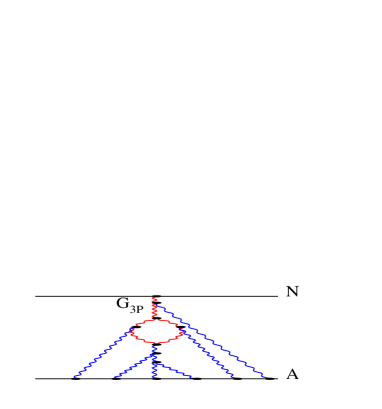
“Fan” diagrams	First enhanced diagram

Figure 34: The first correction to our approach.

Direct calculation of the ratio

$$\frac{Enhanced\,\,\,\,diagram}{``Fan"\,\,\,\,diagram}\,\,\,\,\Longrightarrow|_{s\rightarrow\infty}\frac{G^{2}_{3P}}{2\,\alpha^{\prime}_{P}}\,\,y^{2}$$ (4.68)

shows that in our approach we have achieved reasonable accuracy only for sufficiently small values of the triple Pomeron vertex. In pQCD (see Eq. (1.8) and Eq. (1.9) ) one can see that the ratio of Eq. (4.68) is proportional to $\alpha^{2}_{S}y^{2}$, and, therefore, it appears that we can neglect the contribution of the enhanced diagram in the wide region of energy $y=\ln s<1/\alpha_{S}$. However, the numerical parameters of our fit (see section 2.6 ) gives $G^{2}_{3P}$/$2\,\alpha^{\prime}_{P}$ $\,\,\approx\,\,1$.

References

- [1] D. Yu. Ivanov et al., Phys. Rev. D58 (1998) 074010, hep-ph/9804443.
- [2] E.A. Kuraev, L.N. Lipatov and V.S. Fadin, Sov. Phys. JETP 45 (1977) 199 ; Ya.Ya. Balitskii and L.V. Lipatov:Sov. J. Nucl. Phys. 28 (1978)822; L.N. Lipatov: Sov. Phys. JETP 63 (1986) 904.
- [3] V.S. Fadin and L.N. Lipatov, Phys. Lett. B429 (1998) 127; M. Ciafaloni and G. Camici, Phys. Lett. B412 (1997) 396; M. Ciafaloni, Phys. Lett. B429 (191998) 363; M. Ciafaloni and G. Camici, Phys. Lett. B430 (1998) 349; D.A. Ross, Phys. Lett. B431 (1998) 161; Yu.V. Kovchegov and A.H. Mueller, Phys. Lett. B439 (1998) 428; E.Levin, Nucl. Phys. B545 (1999) 481,hep-ph/9806228 ; N. Armesto, J. Bartels and M.A. Braun, Phys. Lett. B442 (1998) 459,hep-ph/9808340; G.P. Salam,JHEP 9807 (1998) 19.
- [4] A. Donnachie and P.V. Landshoff, Nucl. Phys. B244 (1984) 322, Nucl. Phys. B267 (1986) 690, Phys. Lett. B296 (1992) 227, Z. Phys. C61 (1994) 139.
- [5] K.G. Boreskov, A. Capella, A.B. Kaidalov and J. Tran Thanh Van,Phys. Rev. D47, 919 (1993); A.B. Kaidalov, L.A. Ponomarev and K.A. Ter–Martirosyan, Sov.J.Nucl.Phys. 44,(1986) 486; A. Capella, J. Kaplan and J. Tran Thanh Van, Nucl Phys. B105 (1976) 333.
- [6] E. Gotsman,E. Levin and U. Maor, Phys. Lett. B452 (1999) 287, Phys. Rev. D49 (1994) 4321, Phys. Lett. B304 (1993) 199, Z. Phys. C57 (1993) 672.
- [7] A. Schwimmer, Nucl. Phys. B94 (1975) 445.
- [8] E. Levin, Phys. Rev. D49 (1994) 4469.
-
[9]
A.M. Cooper-Sarkar, R.C.E. Devenish and A. De
Roeck: Int.J.Mod.Phys. A13, (1998) 3385;
H.Abramowicz and A. Caldwell: HERA Collider Physics DESY-98-192, hep-ex/9903037, Rev. Mod. Phys. (in press ). -
[10]
H1 Collaboration: S. Aid et al., Nucl. Phys. B472 (1996) 3;
ZEUS Collaboration: M. Derrick et al., Phys. Lett. B350 (1996) 120. -
[11]
E.M. Levin and L.L. Frankfurt, JETP Letters 3 (1965) 652;
H.J. Lipkin and F. Scheck, Phys. Rev. Lett. 16 (1966) 71;
J.J.J. Kokkedee, The Quark Model , NY, W.A. Benjamin, 1969. -
[12]
L. V. Gribov,
E. M. Levin and M. G. Ryskin, Phys.Rep. 100, 1 (1983);
A.H. Mueller and J. Qiu, Nucl. Phys. B268, 427 (1986);
E.M. Levin and M.G. Ryskin, Phys. Rept. 189 (1990) 267;
E. Laenen and E. Levin, Ann. Rev. Nucl. Part. 44 (1994) 199 and references therein;
L. McLerran and R. Venugopalan, Phys. Rev. D49 (1994) 2233,3352, D50 (1994) 2225, D53 (1996) 458, D59 (1999) 094002;
A.L. Ayala, M.B. Gay Ducati and E.M. Levin, Nucl. Phys. B493, 305 (1997), B510, 355 (1998);
Yu. Kovchegov, Phys.Rev.D54 (1996) 5463; D55 (1997) 5445; D60 (1999) 034008;
A.H. Mueller, CU - TP - 941, hep-ph/9906322, CU - TP - 937, hep-ph/9904404. -
[13]
E. Gotsman,E. Levin and U. Maor, Nucl. Phys. B493 (1997)
354; Phys. Lett. B 425(1998) 369;
E. Gotsman, E. Levin, U. Maor and E. Naftali, Nucl. Phys. B539,
(1999) 535;
A.H. Mueller, Small and Diffraction Scattering, DIS’98, eds. Ch. Coremans and R. Roosen, WS,1998, Parton Saturation at Small and in Large Nuclei, CU-TP-937-99, hep-ph/9904404;
K. Golec-Biernat and M. Wüsthoff, Phys. Rev. D59 (1999) 014017, Saturation in Diffractive Deep Inelastic Scattering, DTP-99-20,hep-ph/9903358. -
[14]
J. Bartels, Z. Phys. C60 (1993) 471; Phys. Lett. B298 (1992) 589;
E.M. Levin, M.G. Ryskin and A.G. Shuvaev, Nucl. Phys. B387 (1992) 204. -
[15]
G. Veneziano, Phys. Lett. B52 (1974) 220, Nucl. Phys. B74 (1974) 365;
G. Marchesini and G. Veneziano, Phys. Lett. B56 (1975) 271;
M.Ciafaloni,G. Marchesini and G. Veneziano, Nucl. Phys. B98 (1975) 308. - [16] For Reggeon Field Theory (RFT), see, for instance, Regge Theory of Low- Hadronic Interaction, edited by L. Caneschi, Current Physics Sources and Comments Series ( North-Holland, Amsterdam, 1989 ),
-
[17]
R.J. Glauber,Lectures in Theoretical Physics. Ed. W.E. Britten
N.Y., Int.Publ. 1959,v.1,p.315.
V.N. Gribov,JETP 56(1969) 892, 57 (1969) 1306. - [18] A. Capella, A. Kaidalov and J. Tran Thanh Van, Heavy Ion Phys. 9 (1999) 169, hep-ph/9903244 and references therein.
- [19] A. Capella, U. Sukhatme, C-I Tan anf J. Tran Tranh Van, Phys. Rept. 236 (1994) 225 and references therein.
- [20] A.B. Kaidalov, Nucl. Phys. A525 (19991) 39.
- [21] K.G. Boreskov and A.B. Kaidalov, Acta Phys. Plon. B20 (1989) 397; Sov. J. Nucl. Phys. 48 (1988) 357.
- [22] G.A. Winbow, Phys. Rev. Lett. 40 (1978) 619; Phys. Rev. D15 (1977) 303.
- [23] Moshe Moshe, Phys. Rept. 37 (1978) 255 and references therein.
- [24] J. H. Weis, Acta Phys. Plon. B7 (1976) 851.
- [25] L. Caneschi, A. Schwimmer and R. Jengo, Nucl. Phys. B108 (1976) 82.
- [26] E. M. Levin, M.G. Ryskin and N.N. Nikolaev,Z. Phys. C5 ( 1980) 285.
- [27] O.V. Kancheli, JETP Letters 18 (1973) 274.
- [28] E.M. Levin and M. G. Ryskin, JETP Letters 18 (1973) 654; Sov. J. Nucl. Phys. 19 (1974) 669; 20 (1974) 519; 21 (1975) 396.
- [29] J. Koplik and A.H. Mueller,Phys. Let. B58 (1975) 166; Phys. Rev. D12 (1975) 3638.
- [30] A. Capella and A. Krzywicki, Phys. Let. B67 (1977) 331.
-
[31]
A.B. Kaidalov and K. A. Ter Martirosyan, Phys. Let. B117
(1982)
247;
A.B. Kaidalov, K. A. Ter Martirosyan and Yu. M. Shabelsky,Sov. J. Nucl. Phys. 43 (1986) 822. - [32] V.A. Abramovsky, V.N. Gribov and O.V. Kancheli, Sov. J. Nucl. Phys. 18 (1974) 308.
- [33] J. Bartels and M.G. Ryskin, Z.Phys. C76 (1997) 241 and references therein.
- [34] J.D. Bjorken, Int. J. Mod. Phys. A7 ( 1992 ) 4189; Phys. Rev. D47 ( 1993 ) 101.
- [35] J.C. Collins, D.E. Soper and G. Sterman: Nucl. Phys. B308 (1988) 833.
-
[36]
E. Levin, A.D. Martin and M.G. Ryskin, J. Phys. G25 (1999)
1507 and references therein;
A.Rostovtsev, M.G.Ryskin, Phys.Lett. B390 (1997) 375;
E. Gotsman, E. Levin and U. Maor, “The survival probability of large rapidity gaps in a three channel model” hep-ph/9902294, Phys.Rev. D ( in press ), Phys. Lett. B438 (1998) 229, Nucl. Phys. B493 (1997) 354, Phys. Lett. B309 (1993) 199;
R.S.Fletcher, Phys. Lett. B320 (1994) 373. - [37] A.H. Mueller, Phys.Rev. D2 (1970) 2963, D4 (1971) 150.
- [38] Yu. V. Kovchegov, hep-ph/9905214; E. Levin and K. Tuchin, hep-ph/9908317.