UAB-FT-482

KA-TP-2-2000

LC-TH-2000-013

hep-ph/0001254

January 2000

ABSTRACT

We review the one-loop corrections to the partial decay width of sbottom-quark into a top quark and a chargino for the parameter space relevant to the TESLA $e^{+}e^{-}$ linear collider. We present the results available in the literature for the QCD and the Yukawa coupling corrections in a unified framework. In this way a direct comparison of the size of the various corrections is possible.

1 Introduction

Scalar quarks (the SUSY partners of quarks) could be produced at appreciable rates at the TESLA collider. A large amount of work is already avaliable concerning the phenomenology and the radiative corrections of the scalar fermion sector relevant for the linear collider (see e.g. [1, 2, 3, 4, 6, 5, 7, 8] and references therein). With the experimental precision expected at TESLA it will be become necessary to include also the quantum corrections in the theoretical investigations. The largest radiative corrections for the squark sector of the MSSM are associated with the strong interaction. Such QCD corrections have been investigated for the production cross-section [3] and for several other squark observables [4, 6, 5]. However, the electroweak (EW) corrections can also be sizeable and are in general not negligible. This applies in particular to the squarks of the third generation, owing to the large Yukawa couplings of the fermions

$$\lambda_{t}\equiv{h_{t}\over g}={m_{t}\over\sqrt{2}\,M_{W}\,\sin{\beta}}\;\;\;\;\;,\;\;\;\;\;\lambda_{b}\equiv{h_{b}\over g}={m_{b}\over\sqrt{2}\,M_{W}\,\cos{\beta}}\,,$$ (1)

where $\tan\beta$ is the ratio between the vacuum expectation values of the two Higgs bosons doublets, $\tan\beta=v_{2}/v_{1}$. The Yukawa couplings (1) determine the strength of the interactions between quarks and Higgs particles, squarks and higgsinos (the SUSY partners of the quarks and Higgs particles respectively), and part of the interactions between the squarks and Higgs bosons. However, in the case of squarks there are additional interactions originating from the breaking of SUSY, the so-called soft-SUSY-breaking trilinear terms. Although these terms are bounded by the condition that the vacua do not break charge and color, they can be large enough to provide large quantum corrections. Recently, the Yukawa corrections to the production cross-section [7] have received attention.

We have computed the leading electroweak corrections to the partial decay width of a bottom squark into a top quark and a chargino $\Gamma(\tilde{b}\to t\chi^{-})$ [8]. The reasons to choose this concrete channel are at least twofold. First of all it is a process of special interest. The third generation squarks can be the lightest sfermions of the model, owing to the large Yukawa couplings that make their mass decrease when one assumes a common sfermion mass scale at a unification scale, according to the Renormalization Group evolution. Secondly, the third generation squarks are most likely to develop large EW corrections, owing to their large couplings to the Higgs sector. Of course, the neutral channels ($\tilde{t}\to t\chi^{0}$ and $\tilde{b}\to b\chi^{0}$) are equally interesting.

A key point in the computation of observables with $R$-odd external particles is that it is no longer possible to separate between SUSY and non-SUSY corrections. This means that, when making the appropriate renormalization, both the $R$-even and $R$-odd sectors of the theory have to be renormalized. Hence, for the computation of the decay process mentioned above we should perform the renormalization of all the neutralino-chargino sector, together with the gauge and the Higgs sector, which is a rather voluminous task. We have therefore chosen a scenario that allows a simplified treatment: If we assume that the gaugino soft-SUSY-breaking masses are much larger than the higgsino mass parameter $|\mu|$ then we can treat the $\chi^{-}$ appearing in the process as a purely higgsino particle; in this way we can avoid to deal with all the plethora of gauge and gaugino particles in the electroweak sector. Of course this is only a first approximation, but it is already sufficient to demonstrate the importance of the corrections, before performing the full computation. This specification to the leading Yukawa terms is meaningful only in the higgsino approximation, where the soft-SUSY-breaking gaugino masses have to fulfill the relation

$$M^{\prime},M\gg\{|\mu|,M_{W}\}\,\,,$$

with the lightest chargino as pure higgsino, that is

$$\chi^{-}_{1}={\tilde{h}^{-}}\,\,,\,\,m_{\chi^{-}_{1}}\simeq|\mu|\,\,,\,\,\chi^{-}_{2}=\tilde{w}^{-}\,\,,\,\,m_{\chi^{-}_{2}}\simeq M\,\,.$$ (2)

2 Tree-level relations

The tree-level Lagrangian for the top-sbottom-chargino interactions reads

$${\cal L}_{t{\tilde{b}}\chi}=-g\,{\tilde{b}}^{*}_{a}\bar{\chi}^{+}_{i}(A_{+}^{ai}P_{L}+\epsilon_{i}\,A_{-}^{ai}P_{R})t+{\rm h.c.}\,,$$ (3)

where $\epsilon_{i}$ is the sign of the ith chargino eigenvalue $M_{i}\,(i=1,2$ with $|M_{1}|<|M_{2}|$) in the real matrix representation, and the coupling matrices are denoted by

$$A_{+}^{ai}=R_{1a}V_{i1}-\lambda_{b}R_{2a}V_{i2}\,,\ \ \ \ A_{-}^{ai}=-R_{1a}\lambda_{t}U_{i2}\,.$$ (4)

The explicit appearance of the Yukawa couplings (1) in the Lagrangian above requires both the introduction of top and bottom quark mass counterterms (in the on-shell scheme) and also a suitable prescription for the renormalization of $\tan\beta$. We denote by $m_{\tilde{b}_{a}}\,(a=1,2)$, with $m_{\tilde{b}_{1}}<m_{\tilde{b}_{2}}$, the two sbottom mass eigenvalues. The sbottom mixing angle $\theta_{\tilde{b}}$ is defined by the transformation relating the weak-interaction (${\tilde{b}}^{\prime}_{a}={\tilde{b}}_{L},{\tilde{b}}_{R}$) and the mass eigenstate (${\tilde{b}}_{a}={\tilde{b}}_{1},{\tilde{b}}_{2}$) squark bases:

$${\tilde{b}}^{\prime}_{a}=R_{ab}\,{\tilde{b}}_{b}\,\,;\,\,\,\,R=\left(\begin{array}[]{cc}\cos\theta_{\tilde{b}}&-\sin\theta_{\tilde{b}}\\ \sin\theta_{\tilde{b}}&\cos\theta_{\tilde{b}}\end{array}\right)\,;$$ (5)

$R$ is the matrix appearing in eq. (4). By this basis transformation, the sbottom mass matrix,

$${\cal M}_{\tilde{b}}^{2}=\left(\begin{array}[]{cc}M_{\tilde{b}_{L}}^{2}+m_{b}^{2}+\cos{2\beta}(-{1\over 2}+{1\over 3}\,s_{W}^{2})\,M_{Z}^{2}&m_{b}\,(A_{b}-\mu\tan\beta)\\ m_{b}\,(A_{b}-\mu\tan\beta)&M_{\tilde{b}_{R}}^{2}+m_{b}^{2}-{1\over 3}\,\cos{2\beta}\,s_{W}^{2}\,M_{Z}^{2}\,,\end{array}\right)\,,$$ (6)

becomes diagonal: $R^{\dagger}\,{\cal M}_{\tilde{b}}^{2}\,R={\rm diag}\left\{m_{\tilde{b}_{2}}^{2},m_{\tilde{b}_{1}}^{2}\right\}\,.$

Our aim is to compute the radiative corrections in an on-shell renormalization scheme; hence, the input parameters are physical observables (i.e. the physical masses $m_{\tilde{b}_{2}},m_{\tilde{b}_{1}}$, …) rather than formal parameters in the Lagrangian (i.e. the soft-SUSY-breaking parameters $M_{\tilde{b}_{L}}^{2},A_{b}$, … in eq. (6)). Specifically, we use the following set of independent parameters for the squark sector:

$$(m_{\tilde{b}_{1}},m_{\tilde{b}_{2}},\theta_{\tilde{b}},m_{\tilde{t}_{1}},\theta_{\tilde{t}})\,.$$ (7)

The value of the other stop mass $m_{\tilde{t}_{2}}$ is then determined by $SU(2)_{L}$ gauge invariance. For the numerical study, we shall use a range of bottom-squark masses $300-350\mbox{ GeV}$, relevant for a $\sqrt{s}=800\mbox{ GeV}$ $e^{+}e^{-}$ linear collider. The sbottom and stop trilinear soft-SUSY-breaking terms $A_{b}$ and $A_{t}$ are fixed at the tree-level by the previous parameters as follows:

$$A_{b}=\mu\,\tan\beta+{m_{\tilde{b}_{2}}^{2}-m_{\tilde{b}_{1}}^{2}\over 2\,m_{b}}\,\sin{2\,\theta_{\tilde{b}}}\,;\ \ \ \ A_{t}=\mu\,\cot\beta+{m_{\tilde{t}_{2}}^{2}-m_{\tilde{t}_{1}}^{2}\over 2\,m_{t}}\,\sin{2\,\theta_{\tilde{t}}}\,.$$ (8)

We impose the approximate (necessary) condition

$$A_{q}^{2}<3\,(m_{\tilde{t}}^{2}+m_{\tilde{b}}^{2}+M_{H}^{2}+\mu^{2})\,,$$ (9)

where $m_{\tilde{q}}$ is of the order of the average squark masses for $\tilde{q}=\tilde{t},\tilde{b}$, to avoid colour-breaking minima in the MSSM Higgs potential [12]. Of course the relation (8) receives one-loop corrections. However, since these parameters do not enter the tree-level expressions, these effects translate into two-loop corrections to the process under study. The bound (9) translates into a stringent constrain to the sbottom-quark mixing angle for moderate and large values of $\tan\beta\mbox{ \raisebox{-4.0pt}{${\stackrel{{\scriptstyle\textstyle>}}{{\sim}}}$} }10$: with an approximate limit $|\mu|\mbox{ \raisebox{-4.0pt}{${\stackrel{{\scriptstyle\textstyle>}}{{\sim}}}$} }80\mbox{ GeV}$ from the negative output of the chargino search at LEP, the condition (9) can only be satisfied by a cancellation of the two terms in (8) which is easily spoiled when $\theta_{\tilde{b}}$ is varied. The right hand side of eq. (9) is not rigorous; so we will present results also when this bound is not satisfied, but we will clearly mark these regions. With the use of the bound (9) also the squark-squark-Higgs-boson couplings are restricted. This is a welcome feature, since these couplings can in general be very large, eventually spoiling perturbativity.

It is clear that the radiative corrections to the process $\tilde{b}_{a}\rightarrow t\,\chi^{-}_{i}$ will only be of practical interest in the region where it also has a large tree-level branching ratio. There are several channels ($\tilde{b}_{a}\to b\tilde{g}$, $\tilde{b}_{a}\rightarrow b\,\chi^{0}_{\alpha}$, $\tilde{b}_{2}\rightarrow\tilde{b}_{1}h^{0}$, …) that contribute to the sbottom-quark decay width. The gluino channel, if kinematically avaliable, saturates the total width, so in order to have an appreciable branching ratio $\tilde{b}_{a}\rightarrow t\,\chi^{-}_{i}$ we start out assuming that the gluino is much heavier than the squarks $m_{\tilde{g}}>m_{\tilde{b}_{a}}$, $a$=1, 2. Neutralino masses, on the other hand, are related to chargino masses; thus, no additional conditions can be imposed on this side.

Let us define the branching ratio for the decay under investigation:

$$BR_{0}(\tilde{b}_{a}\rightarrow t\,\chi^{-}_{1})={\Gamma_{0}(\tilde{b}_{a}\rightarrow\chi^{-}_{1}\,t)\over\Gamma_{0}^{T}(\tilde{b}_{a})}\,\,,$$ (10)

where $\Gamma_{0}^{T}(\tilde{b}_{a})$ is the total $\tilde{b}_{a}$ decay width. This branching ratio is maximized in a scenario where the lightest chargino is higgsino-dominated and $\tan\beta$  is of low–moderate value. For large $\tan\beta\mbox{ \raisebox{-4.0pt}{${\stackrel{{\scriptstyle\textstyle>}}{{\sim}}}$} }40$, $\Gamma_{0}^{T}$ is dominated by the neutral higgsino contribution.

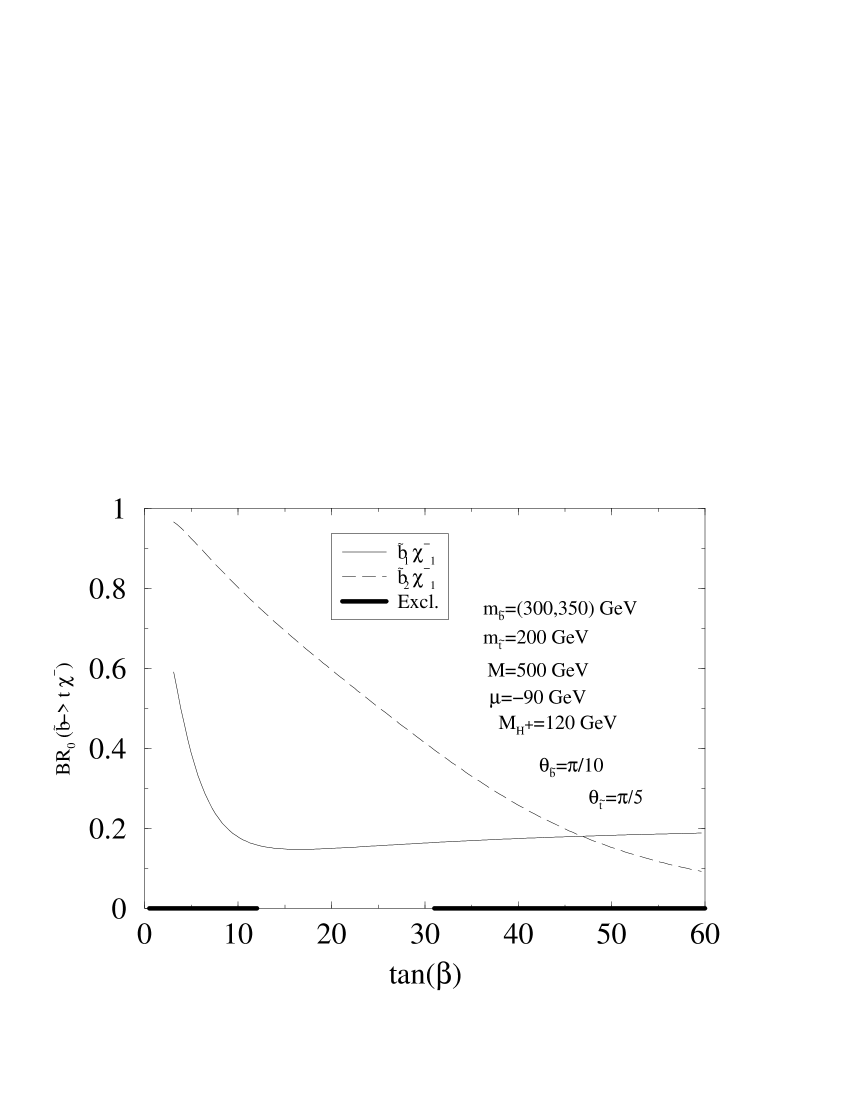
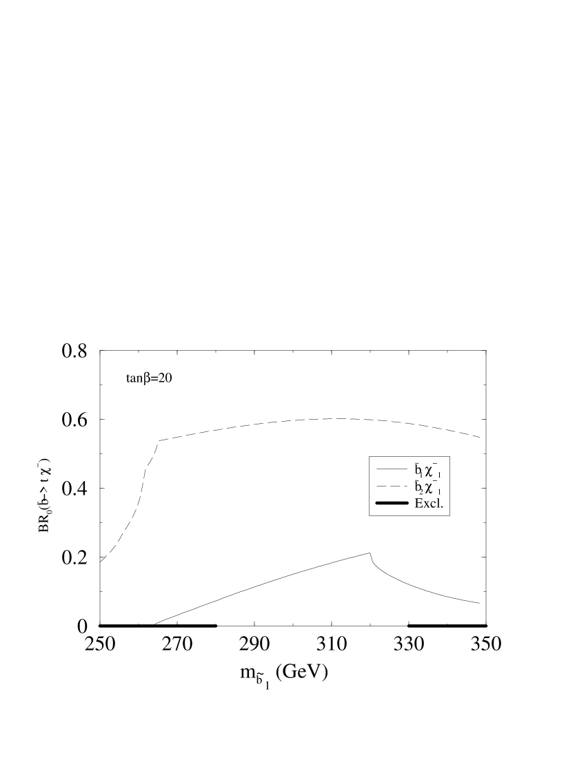
(a)	(b)
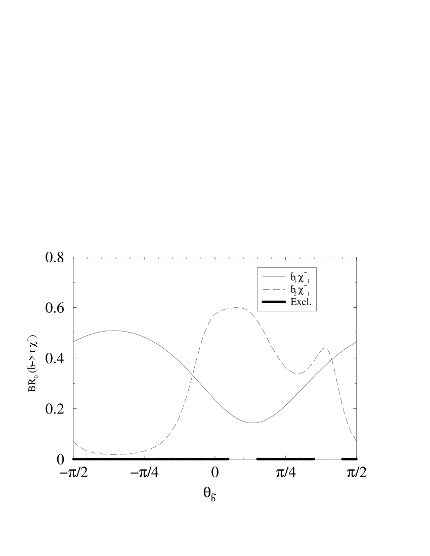
(c)

Figure 1: (a) The branching ratio of  $\tilde{b}_{a}\rightarrow\chi_{1}^{-}\,t$  as a function of $\tan\beta$ for the various decays $a=1,2$ with $m_{\tilde{b}_{1}}<m_{\tilde{b}_{2}}$; (b) As in (a), but as a function of $m_{\tilde{b}_{1}}$; (c) As in (a), but as a function of $\theta_{\tilde{b}}$. The marked parts of the abscissa in both figures are excluded by the condition (9). The fixed parameters for (a) and (b) are given in the frame.

Figure 1 displays the value of the branching ratio (10) as a function of $\tan\beta$, $m_{\tilde{b}_{1}}$ and $\theta_{\tilde{b}}$, for given values of the other parameters. It can be seen that low $\tan\beta$  values enhance the branching ratio. From now on we will concentrate in the region of $\tan\beta\simeq 20$; with this typical value the branching ratio still is appreciably high, whereas the electroweak corrections can be enhanced by means of the bottom Yukawa coupling (1). In Fig. 1(b) we can see the thresholds for opening the Higgs channels, namely $\tilde{b}_{2}\rightarrow\tilde{b}_{1}\,h^{0}$ (at the left end of the figure) and $\tilde{b}_{1}\rightarrow\tilde{t}_{1}\,H^{-}$ (at its right end). When these channels are open, they tend to decrease the branching ratio (10) to undetectable small values. The large decay width into Higgs bosons results from large values for the $A$ parameters (8) in these kinematical region. Of course one could fix the input parameters (7) in such a way that $A_{\{t,b\}}$ are small in one of these regions (say at $m_{\tilde{b}_{1}}$ light), but at the price of making them large at its central value and even larger at the other end. This effect is also seen in Fig. 1(c), as the $A$ parameters are related to the angle trough (8). Note that the allowed range of $\theta_{\tilde{b}}$ is rather narrow, so that the physical bottom squark mass eigenstates basically coincide with the left- and right-handed chiral electroweak eigenstates.

3 One-loop corrections

The QCD one-loop corrections were originally computed in Refs.[6, 5]. Our QCD results presented here were computed independently and are in full agreement with those of [6, 5]. We include them in our discussion, for comparison with the residual ones, within the same scenario in which we computed the Yukawa part. The Yukawa corrections were first presented in [8]. The full analytical results of the corrections can be found in [6, 5, 8]. The QCD corrections contain all the gluon and gluino exchange diagrams, together with the soft and hard gluon bremsstrahlung, and the Yukawa corrections contain the diagrams in which Higgs bosons and higgsinos are exchanged. We use the on-shell renormalization scheme with the input parameters described in (7). The renormalization of the $\tan\beta$ parameter (necessary for the weak corrections) is fixed in such a way that the decay width $\Gamma(H^{+}\to\tau^{+}\nu_{\tau})$ does not receive quantum corrections [9]. The $\mu$ parameter is renormalized in analogy to fermion mass renormalization, since in our approximation it is the mass of the chargino involved in the decay. The bottom-squark mixing angle has to be renormalized as well. At variance with the other parameters appearing in our process, it is still not clear how this angle could be measured. Hence we treat $\theta_{\tilde{b}}$ as a formal parameter and impose as a renormalization condition that it is not shifted by loop corrections from the mixed $\tilde{b}_{1}\tilde{b}_{2}$ self-energy [8].

The quantity under study will be the relative one-loop correction defined as:

$$\delta^{ai}=\frac{\Gamma(\tilde{b}_{a}\to t\chi^{-}_{i})-\Gamma_{0}(\tilde{b}_{a}\to t\chi^{-}_{i})}{\Gamma_{0}(\tilde{b}_{a}\to t\chi^{-}_{i})}\,\,.$$ (11)

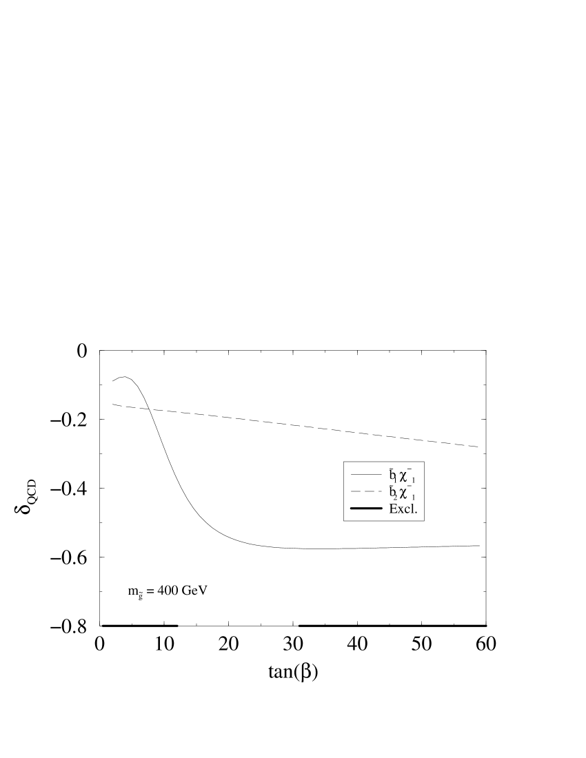
(a) (b)

Figure 2: The correction $\delta^{ai}_{QCD}$ to the decay width $\tilde{b}_{a}\rightarrow t\,\chi^{-}$ as a function of (a) $\tan\beta$  and (b) the higgsino mass parameter $\mu$. Set of inputs as in Fig. 1.

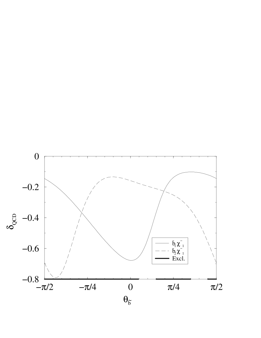
Figure 3: The correction $\delta^{ai}_{QCD}$ as a function of $\theta_{\tilde{b}}$. Inputs as in Fig. 1.

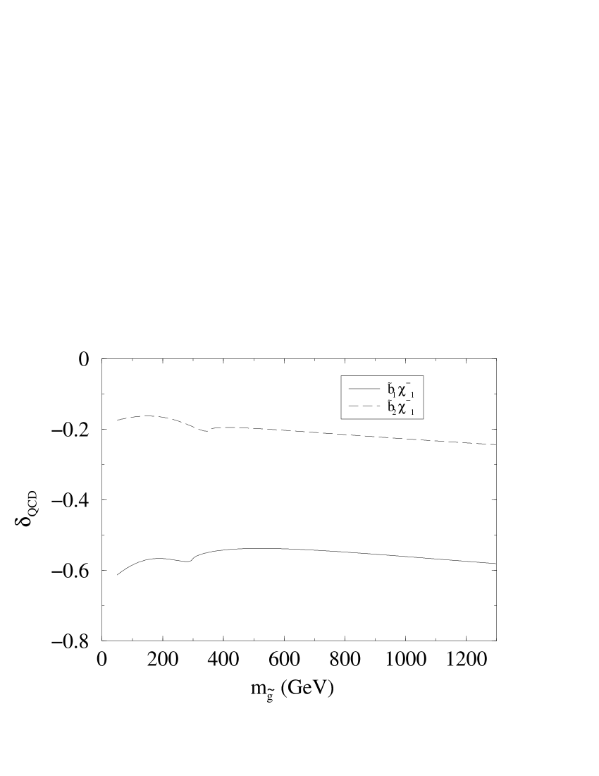
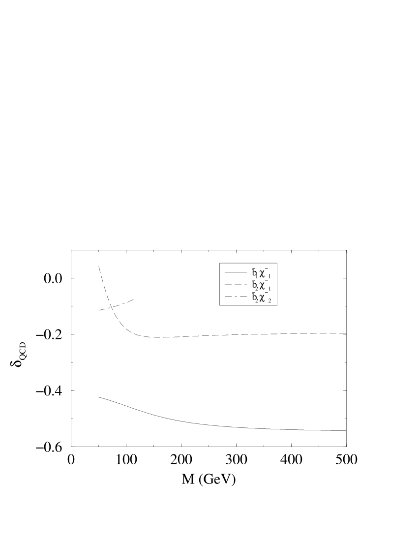
(a) (b)

Figure 4: The correction $\delta^{ai}_{QCD}$ as a function of (a) the gluino mass $m_{\tilde{g}}$  and (b) the gaugino mass parameter $M$. Set of inputs as in Fig. 1.

We start with the QCD corrections shown in Figs. 2-4. For the numerical evaluation we use $\alpha_{s}(m_{\tilde{b}_{a}})$, using the one-loop MSSM $\beta$-function, but, for the $m_{\tilde{b}_{a}}$ we use, it is basically the 4-flavour SM $\beta$-function, as the scale is almost always below the threshold of coloured SUSY particles (and top quark). In Fig. 2 we can see the evolution with $\tan\beta$  and $\mu$, which are the most interesting cases. The corrections are large ($>10\%$) and vary slowly for large values of $\tan\beta$ ($\mbox{ \raisebox{-4.0pt}{${\stackrel{{\scriptstyle\textstyle>}}{{\sim}}}$} }20$). We remark that for $\mu<-120\,\mbox{ GeV}$ and $\tan\beta>20$ the corrections can be very large near the phase space limit of the lightest sbottom decay. However, this effect has nothing to do with the phase space exhaustion, but rather with the presence of a dynamical factor which goes to the denominator of $\delta$ in eq. (11). That factor is fixed by the structure of the interaction Lagrangian of the sbottom decay into charginos and top; for the parameters in Fig. 2, it turns out to vanish nearly at the phase space limit in the case of the lightest sbottom ($\tilde{b}_{1}$) decay. However, this is not so either for the heaviest sbottom ($\tilde{b}_{2}$) or for $\mu>120\,\mbox{ GeV}$ as it is patent in the same figure. The different evolution that exhibit the corrections of the two sbottoms has more relation with the electroweak nature of the process than with the purely QCD loops. For small angles $\theta_{\tilde{b}}$ and $\theta_{\tilde{t}}$ the squarks are nearly chiral, namely

$$\tilde{b}_{1}\simeq\tilde{b}_{R}\,\,\,\,,\,\,\,\tilde{b}_{2}\simeq\tilde{b}_{L}\,\,\,\,,\,\,\,\tilde{t}_{1}\simeq\tilde{t}_{R}\,\,\,\,,\,\,\,\tilde{t}_{2}\simeq\tilde{t}_{L}\,\,\,,$$ (12)

and thus their very different couplings to charginos translate into very different behaviours of (11) with $\tan\beta$  and $\mu$. In fact, the sbottom mixing angle plays a crucial role, as seen in Fig. 3; we also see, however, that its value is highly constrained by the condition (9). We should also comment on the effect of the gaugino mass parameter $M$ and the gluino mass in Fig. 4. The gluino evolution is rather flat once the pseudo-thresholds of $\tilde{b}_{a}\rightarrow b\,\tilde{g}$ are passed; thus, even if the gluino were much heavier than the squarks it would have an effect on the sbottom decay while at the same time it would prevent the otherwise dominant decay $\tilde{b}_{a}\to b\tilde{g}$. The correction is saturated for the gaugino mass parameter $M\mbox{ \raisebox{-4.0pt}{${\stackrel{{\scriptstyle\textstyle>}}{{\sim}}}$} }200\mbox{ GeV}$. Therefore the effects computed here can be compared with the ones obtained in the higgsino approximation discussed below. Finally, we point out the possible existence of non-decoupling effects in the QCD part. In [6] it is shown that there exist a non-decoupling effect at large gluino masses, however this effect is numerically small and is not the one reflected in Fig. 4(a). The origin of the effect is related to the breaking of SUSY, specifically to the fact that the chargino coupling has a renormalization group evolution which is different to that of the gauge coupling in a non-SUSY world, the difference being sensitive to the splitting among the various SUSY scales – e.g. the scales of the squark and gluino masses.

The other parameters of the model present a rather mild effect on the corrections for squark masses in the ballpark of several hundreds of GeV. In summary the QCD corrections on the decay $\tilde{b}_{a}\rightarrow t\,\chi^{-}_{i}$ are large ($\simeq-20\%$ for $\tilde{b}_{2}$, $\simeq-60\%$ for $\tilde{b}_{1}$) and negative for values of the parameter space relevant to TESLA energies, with a higgsino-like chargino and moderate or large values of $\tan\beta$.

We now turn to the discussion of the Yukawa corrections where also non-decoupling effects may come into play. They have a different origin as compared to the pure QCD ones but they are also triggered by SUSY-breaking and can be numerically important. We remind that, in the computation of the Yukawa corrections, the higgsino approximation, eq. (2), was used, and so only the lightest chargino is avaliable for the decay. In the relevant large $\tan\beta$ segment under consideration, namely

$$20\mbox{ \raisebox{-4.0pt}{${\stackrel{{\scriptstyle\textstyle<}}{{\sim}}}$} }\tan\beta\mbox{ \raisebox{-4.0pt}{${\stackrel{{\scriptstyle\textstyle<}}{{\sim}}}$} }40\,,$$ (13)

the bottom quark Yukawa coupling $\lambda_{b}$ is comparable to the top quark Yukawa coupling $\lambda_{t}$. Even though the extreme interval $40<\tan\beta<60$ can be tolerated by perturbation theory, we shall confine ourselves to the moderate range (13). This is necessary to preserve the condition (9) for the typical set of sparticle masses used in our analysis.

(a)	(b)

Figure 5: (a) The SUSY-EW corrections (11) as a function of $m_{\tilde{t}_{1}}$; (b) As in (a), but as a function of $m_{\tilde{b}_{1}}$. Rest of inputs as in Fig. 1.

(a)	(b)

Figure 6: (a) Evolution of the SUSY-EW corrections as a function of the sbottom mixing angle, ${\theta}_{\tilde{b}}$, within its allowed range; (b) As in (a), but as a function of the stop mixing angle, ${\theta}_{\tilde{t}}$. Remaining inputs are as in Fig. 1.

(a)	(b)

Figure 7: (a) The SUSY-EW correction as a function of $\tan\beta$; (b) As in (a), but as a function of $\mu$. Rest of inputs and notation as in Fig. 1.

The corresponding corrections $\delta^{ai}$ (11) are shown in Figs. 5(a) and 5(b) as a function of the lightest stop and sbottom masses, respectively. The precise value of the lightest stop mass is an important parameter to determine the corrections to the lightest sbottom decay width. On the other hand the lightest sbottom mass does not play a major role for the corrections, aside from the presence of various thresholds. The allowed range for the sbottom and stop mixing angles is conditioned by the upper bound on the trilinear couplings and is obtained from eqs. (8) and (9). In the physical $\theta_{\tilde{b}}$ range, the variation of the correction (11) is shown in Fig. 6(a). The large values of the corrections far away from the allowed region (9) are due to the large values of the soft-SUSY-breaking trilinear coupling $A_{b}$ (8). On the other hand, the permitted range for the stop mixing angle $\theta_{\tilde{t}}$ is much larger, and we have plotted the corrections within the allowed region in Fig. 6(b). Note that the sign of the quantum effects for the lightest sbottom decay width changes within the domain of variation of $\theta_{\tilde{t}}$. Finally, we display the evolution of the SUSY-EW effects as a function of $\tan\beta$ (Fig. 7(a)) and of $\mu$ (Fig. 7(b)) within the region of compatibility with the constraint (9).

A few words are in order to explain the origin of the leading electroweak effects. One could expect that they come from the well-known large $\tan\beta$ enhancement stemming from the chargino-stop corrections to the bottom mass (see e.g. Ref. [9]). Nonetheless this is only partially true, since in the present case the remaining contributions can be sizeable enough. One can also think on the SUSY counterpart of the bottom mass counterterm corrections, that is, the finite contributions to the sbottom wave function renormalization constants [8], as an additional leading contribution. Both of these effects are of non-decoupling nature. However the addition of these two kind of contributions does not account for the total behaviour in all of the parameter space. To be more precise, in the region of the parameter space that we have dwelled upon the bottom mass contribution is seen to be dominant only for the lightest sbottom decay and for the lowest values of $\tan\beta$ in the range (13). This is indeed the case in Fig. 6(b) where $\tan\beta=20$ and therefore the bottom mass effect modulates the electroweak correction in this process and $\delta^{11}$ becomes essentially an odd function of the stop mixing angle. This fact is easily understood since, as noted above, sbottoms are nearly chiral – eq. (12) – and the $\tilde{b}_{R}$ is the only one with couples with $\lambda_{b}$ – eq. (4). On the other hand, from Fig. 7(a) it is obvious that the (approximate) linear behaviour with $\tan\beta$ expected from bottom mass renormalization becomes completely distorted by the rest of the contributions, especially in the high $\tan\beta$ end. In short, the final electroweak correction cannot be simply ascribed to a single renormalization source but to the full Yukawa-coupling combined yield.

In general the SUSY-EW corrections to $\Gamma(\tilde{b}_{a}\rightarrow t\,\chi^{-}_{i})$ are smaller than the QCD corrections. The reason why the electroweak corrections are smaller is in part due to the condition (9) restricting our analysis within the $\tan\beta$ interval (13). From Figs. 6 and 7(a) it is clear that outside this interval the SUSY-EW contributions could be much higher and with the same or opposite sign as the QCD effects, depending on the choice of the sign of the mixing angles. Moreover, since we have focused our analysis to sbottom masses accessible to TESLA, again the theoretical bound (9) severely restricts the maximum value of the trilinear couplings and this prevents the electroweak corrections from being larger. This cannot be cured by assuming larger values of $\mu$, because $\mu$ directly controls the value of the (higgsino-like) chargino mass, in the final state in the decay under study.

4 Conclusions

In summary, the MSSM corrections to squark decays into charginos can be significant and therefore must be included in any reliable analysis. The main corrections arise from the strongly interacting sector of the theory (i.e. the one involving gluons and gluinos), but also non-negligible effects may appear from the electroweak sector (characterized by chargino-neutralino exchange) at large (or very small) values of $\tan\beta$. In both cases non-decoupling effects related to the breaking of SUSY may be involved, but it is in the electroweak part where they can be numerically more sizeable. However, for sparticle masses of a few hundred $GeV$ a reliable estimate of the correction requires the calculation of the QCD and also of the complete Yukawa-coupling electroweak contribution. The QCD corrections are negative in most of the MSSM parameter space accessible to TESLA. They are of the order

$$\delta_{QCD}(\tilde{b}_{1}\rightarrow t\,\chi^{-}_{1}) \simeq -60\%$$

$$\delta_{QCD}(\tilde{b}_{2}\rightarrow t\,\chi^{-}_{1}) \simeq -20\%$$

for a wide range of the parameter space (Fig. 2). In certain corners of this space, though, they vary in a wide range of values. EW corrections can be of both signs. Our renormalization prescription uses the mixing angle between squarks as an input parameter. This prescription forces the physical region to be confined within a narrow range when we require compatibility with the non-existence of colour breaking vacua. Within this restricted region the typical corrections vary in the range (Figs. 6, 7)

$$\delta_{EW}(\tilde{b}_{1}\rightarrow t\,\chi^{-}_{1}) \simeq +25\%\mbox{ to }-15\%$$

$$\delta_{EW}(\tilde{b}_{2}\rightarrow t\,\chi^{-}_{1}) \simeq +5\%\mbox{ to }-5\%\,\,,$$

However we must recall that these limits are not rigorous. In the edge of such regions we find the largest EW contributions. We stress that for these decays it is not possible to narrow down the bulk of the electroweak corrections to just some simple-structured leading terms.

The present study has an impact on the determination of squark parameters at TESLA. The squark masses used in it would be available already for TESLA running at a center of mass energy of $800\mbox{ GeV}$. The large corrections found from both the QCD and the EW (Yukawa) sector, make this calculation necessary, not only for prospects of precision measurements in the sbottom-chargino-neutralino sectors, but also for a reliable first determination of their parameters.

References

-
[1]
A. Bartl et al., Z. Phys. C76 (1997) 549,
hep-ph/9701336;
H. Eberl, S. Kraml, W. Majerotto, A. Bartl, W. Porod, hep-ph/9909378;
M. Berggren, R. Keranen, H. Nowak, A. Sopczak, hep-ph/9911345. -
[2]
A. Bartl, et al.,
Phys. Lett. B435 (1998) 118, hep-ph/9804265;
ibid. B460 (1999) 157,
hep-ph/9904417;
A. Djouadi, J.L. Kneur, G. Moultaka, hep-ph/9903218. - [3] H. Eberl, A. Bartl, W. Majerotto, Nucl. Phys. B472 (1996) 481, hep-ph/9603206.
-
[4]
A. Bartl et al., Phys. Lett. B373 (1996) 117,
hep-ph/9508283;
A. Djouadi, W. Hollik, C. Junger, Phys. Rev. D54 (1996) 5629, hep-ph/9605340;
W. Beenakker, R. Hopker, T. Plehn, P. M. Zerwas, Z. Phys. C75 (1997) 349, hep-ph/9610313;
A. Arhrib, A. Djouadi, W. Hollik, C. Jünger, Phys. Rev. D57 (1998) 5860, hep-ph/9702426;
A. Bartl et al., Phys. Lett. B419 (1998) 243, hep-ph/9710286; Phys. Rev. D59 (1999) 115007. - [5] S. Kraml, H. Eberl, A. Bartl, W. Majerotto, W. Porod, Phys. Lett. B 386 (1996) 175, hep-ph/9605412.
- [6] A. Djouadi, W. Hollik, C. Jünger, Phys. Rev. D 55 (1997) 6975, hep-ph/9609419.
- [7] H. Eberl, S. Kraml, W. Majerotto, JHEP 05 (1999) 016, hep-ph/9903413.
- [8] J. Guasch, W. Hollik, J. Solà, Phys. Lett. B437 (1998) 88, hep-ph/9802329.
- [9] J.A. Coarasa, D. Garcia, J Guasch, R.A. Jiménez, J. Solà, Eur. Phys. J. C2 (1998) 373.
- [10] J. Guasch, J. Solà, Z. Phys. C 74 (1997) 337, hep-ph/9603441.
- [11] J. Guasch, Ph.D. Thesis, Universitat Autònoma de Barcelona, 1999, hep-ph/9906517.
-
[12]
J.M. Frère, D.R.T. Jones, S. Raby, Nucl. Phys.
B 222 (1983) 11;
M. Claudson, L. Hall, I. Hinchliffe, Nucl. Phys. B 228 (1983) 501;
C. Kounnas, A.B. Lahanas, D.V. Nanopoulos, M. Quirós, Nucl. Phys. B 236 (1984) 438;
J.F. Gunion, H.E. Haber, M. Sher, Nucl. Phys. B 306 (1988) 1. - [13] T. Plehn, W. Beenakker, in Quantum Effects in the Minimal Supersymmetric Standard Model, Barcelona, Spain, 9-13 Sep 1997, World Scientific, ed. Joan Solà, pg. 244.