Anomaly Mediated SUSY Breaking at the LHC

Frank E. Paige^a and James Wells^b

^aPhysics Department, Brookhaven National Laboratory, Upton, NY 11973

^bPhysics Department, University of California, Davis, CA 95616

Anomaly Mediated SUSY Breaking models are reviewed. Possible signatures at the LHC for one case of the minimal realistic model are examined.

Introduction

The signatures for SUSY at the LHC depend very much on the SUSY masses, which presumably result from spontaneous SUSY breaking. It is not possible to break SUSY spontaneously using just the MSSM fields; instead one must do so in a hidden sector and then communicate the breaking through some interaction. In supergravity models, the communication is through gravity. In gauge mediated models it is through gauge interactions; the gravitino is then very light and can play an important role. Simple examples of both have been discussed previously. A third possibility is that the hidden sector does not have the right structure to provide masses through either mechanism; then the leading contributions come from a combination of gravity and anomalies. This is known as Anomaly Mediated SUSY Breaking (AMSB), and it predicts a different pattern of masses and signatures.

Anomaly-Mediated Supersymmetry Breaking

In the supersymmetric standard model there exist AMSB contributions to the soft mass parameters that arise via the superconformal anomaly [1, 2]. The effect can be understood by recognizing several important features of supersymmetric theories. First, supersymmetry breaking can be represented by a chiral superfield $\Phi=1+m_{3/2}\theta^{2}$ which also acts as a compensator for super-Weyl transformations. Treating $\Phi$ as a spurion, one can transform a theory into a super-conformally invariant theory. Even if a theory is superconformal at the outset (i.e., no dimensionful couplings), the spurion $\Phi$ is employed since the quantum field theory requires a regulator that implies scale dependence (Pauli-Villars mass, renormalization scale in dimensional reduction, etc.). To preserve scale invariance the renormalization scale parameter $\mu$ in a quantum theory then becomes $\mu/\sqrt{\Phi^{\dagger}\Phi}$. It is the dependence of the regulator on $\Phi$ that induces supersymmetry breaking contributions to the scalars and gauginos.

The anomaly induced masses can be derived straightforwardly for the scalar masses. The Kähler kinetic terms depend on wave function renormalization as in the following superfield operator,

$$\int d^{2}\theta d^{2}\bar{\theta}Z_{Q}\left(\frac{\mu}{\sqrt{\Phi^{\dagger}\Phi}}\right)Q^{\dagger}Q.$$ (1)

Taylor expanding $Z$ around $\mu$ and projecting out the $FF^{\dagger}$ terms yields a supersymmetry breaking mass for the scalar field $\tilde{Q}$:

$$m_{\tilde{Q}}^{2}=-\frac{1}{4}\frac{d^{2}\ln Z_{Q}}{d(\ln\mu)^{2}}m^{2}_{3/2}=-\frac{1}{4}\left(\frac{\partial\gamma_{Q}}{\partial g}\beta_{g}+\frac{\partial\gamma_{Q}}{\partial y}\beta_{y}\right)m_{3/2}^{2}.$$ (2)

Similar calculations can be done for the gauginos and the $A$ terms:

$$M_{i} = -\frac{g_{i}^{2}}{2}\frac{dg_{i}^{-2}}{d\ln\mu}m_{3/2}=\frac{\beta_{g_{i}}}{g_{i}}m_{3/2},$$ (3)

$$A_{y} = \frac{1}{2}\sum_{a}\frac{d\ln Z_{Q_{a}}}{d\ln\mu}m_{3/2}=-\frac{\beta_{y}}{y}m_{3/2}$$ (4)

where the sum over $a$ includes all fields associated with the Yukawa coupling $y$ in the superpotential.

There are several important characteristics of the AMSB spectrum to note. First, the equations for the supersymmetry breaking contributions are scale invariant. That is, the value of the soft masses at any scale is obtained by simply plugging in the gauge couplings and Yukawa couplings at that scale into the above formulas. Second, the masses are related to the gravitino mass by a one loop suppression. In AMSB $M_{i}\sim m_{3/2}\alpha_{i}/4\pi$, whereas in SUGRA $M_{i}\sim m_{3/2}$. While the AMSB contributions are always present in a theory independent of how supersymmetry breaking is accomplished, they may be highly suppressed compared to standard hidden sector models. Therefore, for AMSB to be the primary source of scalar masses, one needs to assume or arrange that supersymmetry breaking is not directly communicated from a hidden sector. This can be accomplished, for example, by assuming supersymmetry breaking on a distant brane [1]. Finally, the squared masses of the sleptons are negative (tachyonic) because $\beta_{g}>0$ for $U(1)$ and $SU(2)$ gauge groups. This problem rules out the simplest AMSB model based solely on eqs. 2-4.

Given the tachyonic slepton problem, it might seem most rational to view AMSB as a good idea that did not quite work out. However, there are many reasons to reflect more carefully on AMSB. As already mentioned above, AMSB contributions to scalar masses are always present if supersymmetry is broken. Soft masses in the MSSM come for free, whereas in all other successful theories of supersymmetry breaking a communication mechanism must be detailed. In particle, hidden sector models require singlets to give the gauginos an acceptable mass. In AMSB, singlets are not necessary. Also, there may be small variations on the AMSB idea that can produce a realistic spectrum and can have important phenomenological consequences. This is our motivation for writing this note.

Two realistic minimal models of AMSB: mAMSB and DAMSB

As we discussed in the introduction, the pure AMSB model gives negative squared masses for the sleptons, thus breaking electromagnetic gauge invariance, so some additional contributions must be included. The simplest assumption that solves this problem is to add at the GUT scale a single universal scalar mass $m_{0}^{2}$ to all the sfermions’ squared masses. We will call this model mAMSB. The description and many phenomenological implications of this model are given in Refs. [3, 4]. The parameters of the model after the usual radiative electroweak symmetry breaking are then

$$m_{0},\quad m_{3/2},\quad\tan\beta,\quad\mathop{\rm sgn}\mu=\pm.$$

This model has been implemented in ISAJET 7.48 [5]; a pre-release version of ISAJET has been used to generate the events for this analysis.

For this note the AMSB parameters were chosen to be

$$m_{0}=200\,{\rm GeV},\quad m_{3/2}=35\,{\rm TeV},\quad\tan\beta=3,\quad\mathop{\rm sgn}\mu=+$$

For this choice of parameters the slepton squared masses are positive at the weak scale, but they are still negative at the GUT scale. This means that charge and color might be broken (CCB) at high temperatures in the early universe. However, at these high energies there are also large finite temperature effects on the mass, which are positive (symmetry restoration occurs at higher $T$). In fact, a large class of SUSY models with CCB minima naturally fall into the correct SM minimum when you carefully follow the evolution of the theory from high T to today. If CCB minima are excluded at all scales, then the value of $m_{0}$ must be substantially larger, so the sleptons must be quite heavy.

The masses from ISAJET 7.48 for this point are listed in Table 1. The mass spectrum has some similarity to that for SUGRA Point 5 studied previously [6, 7]: the gluino and squark masses are similar, and the decays ${\tilde{\chi}}_{2}^{0}\to{\tilde{\ell}}\ell$ and ${\tilde{\chi}}_{2}^{0}\to{\tilde{\chi}_{1}^{0}}h$ are allowed. Thus, many of the techniques developed for Point 5 are applicable here. But there are also important differences. In particular, the ${\tilde{\chi}}_{1}^{\pm}$ is nearly degenerate with the ${\tilde{\chi}_{1}^{0}}$, not with the ${\tilde{\chi}}_{2}^{0}$. The mass splitting between the lightest chargino and the lightest neutralino must be calculated as the difference between the lightest eigenvalues of the full one-loop neutralino and chargino mass matrices. The mass splitting is always above $m_{\pi^{\pm}}$, thereby allowing the two-body decays $\chi^{\pm}_{1}\to\chi^{0}_{1}+\pi^{\pm}$ [3, 8]. Decay lifetimes of $\chi^{\pm}$ are always less than 10 cm over mAMSB parameter space, and are often less than 1 cm.

Another unique feature of the spectrum is the near degeneracy of the $\tilde{\ell}_{L}$ and $\tilde{\ell}_{R}$ sleptons. The mass splitting is [3]

$$m^{2}_{{\tilde{\ell}}_{L}}-m^{2}_{{\tilde{\ell}}_{R}}\simeq 0.037\left(-m^{2}_{Z}\cos 2\beta+M^{2}_{2}\ln\frac{m_{{\tilde{\ell}}_{R}}}{m_{Z}}\right).$$ (5)

There is no symmetry requiring this degeneracy, but rather it is an astonishing accident and prediction of the mAMSB model.

It is instructive to compare the masses from ISAJET with those calculated in Ref.  to provide weak-scale input to ISAJET. These masses are listed in the right hand side of Table 1. Since the agreement is clearly adequate for the purposes of the present study, no attempt has been made to understand or resolve the differences. It is clear, however, that if SUSY is discovered at the LHC and if masses or combinations of masses are measured with the expected precision, then more work is needed to compare the LHC results with theoretical models in a sufficiently reliable way.

Table 1: Masses of the SUSY particles, in GeV, for the mAMSB model with $m_{0}=200\,{\rm GeV}$, $m_{3/2}=35\,{\rm TeV}$, $\tan\beta=3$, and $\mathop{\rm sgn}\mu=+$ from ISAJET (left side) and from Ref.  (right side) using the ISAJET sign conventions.

Sparticle	mass	Sparticle	mass	Sparticle	mass	Sparticle	mass
$\widetilde{g}$	815			$\widetilde{g}$	852
$\widetilde{\chi}_{1}^{\pm}$	101	$\widetilde{\chi}_{2}^{\pm}$	658	$\widetilde{\chi}_{1}^{\pm}$	98	$\widetilde{\chi}_{2}^{\pm}$	535
$\widetilde{\chi}_{1}^{0}$	101	$\widetilde{\chi}_{2}^{0}$	322	$\widetilde{\chi}_{1}^{0}$	98	$\widetilde{\chi}_{2}^{0}$	316
$\widetilde{\chi}_{3}^{0}$	652	$\widetilde{\chi}_{4}^{0}$	657	$\widetilde{\chi}_{3}^{0}$	529	$\widetilde{\chi}_{4}^{0}$	534
$\widetilde{u}_{L}$	754	$\widetilde{u}_{R}$	758	$\widetilde{u}_{L}$	760	$\widetilde{u}_{R}$	814
$\widetilde{d}_{L}$	757	$\widetilde{d}_{R}$	763	$\widetilde{d}_{L}$	764	$\widetilde{d}_{R}$	819
$\widetilde{t}_{1}$	516	$\widetilde{t}_{2}$	745	$\widetilde{t}_{1}$	647	$\widetilde{t}_{2}$	778
$\widetilde{b}_{1}$	670	$\widetilde{b}_{2}$	763	$\widetilde{b}_{1}$	740	$\widetilde{b}_{2}$	819
$\widetilde{e}_{L}$	155	$\widetilde{e}_{R}$	153	$\widetilde{e}_{L}$	161	$\widetilde{e}_{R}$	159
$\widetilde{\nu}_{e}$	137	$\widetilde{\nu}_{\tau}$	137	$\widetilde{\nu}_{e}$	144	$\widetilde{\nu}_{\tau}$	144
$\widetilde{\tau}_{1}$	140	$\widetilde{\tau}_{2}$	166	$\widetilde{\tau}_{1}$	152	$\widetilde{\tau}_{2}$	167
$h^{0}$	107	$H^{0}$	699	$h^{0}$	98	$H^{0}$	572
$A^{0}$	697	$H^{\pm}$	701	$A^{0}$	569	$H^{\pm}$	575

Another variation on AMSB is deflected AMSB (DAMSB). The idea is based on Ref. [9] who demonstrated that realistic sparticle spectrums with non-tachyonic sleptons can be induced if a light modulus field $X$ (SM singlet) is coupled to heavy, non-singlet vector-like messenger fields $\Psi_{i}$ and $\bar{\Psi}_{i}$:

$$W_{\rm mess}=\lambda_{\Psi}X\Psi_{i}\bar{\Psi}_{i}.$$

To ensure gauge coupling unification we identify $\Psi_{i}$ and $\bar{\Psi}_{i}$ as $5+\bar{5}$ representations of $SU(5)$. When the messengers are integrated out at some scale $M_{0}$, the beta functions do not match the AMSB masses, and the masses are deflected from the AMSB renormalization group trajectory. The subsequent evolution of the masses below $M_{0}$ induces positive mass squared for the sleptons, and a reasonable spectrum can result. Although there may be additional significant parameters associated with the generation of the $\mu$ and $B_{\mu}$ term in the model, we assume for this discussion that they do not affect the spectra of the MSSM fields. The values of $\mu$ and $B_{\mu}$ are then obtained by requiring that the conditions for EWSB work out properly.

The parameters of DAMSB are

$$m_{3/2},\quad n,\quad M_{0},\quad\tan\beta,\quad\mathop{\rm sgn}\mu=\pm$$

where $n$ is the number of $5+\bar{5}$ messenger multiplets, and $M_{0}$ is the scale at which the messengers are integrated out. Practically, the spectrum is obtained by imposing the boundary conditions at $M_{0}$, and then using SUSY soft mass renormalization group equations to evolve these masses down to the weak scale. Expressions for the boundary conditions can be found in Refs. [9, 10], and details on how to generate the low-energy spectrum are given in . The resulting spectrum of superpartners is substantially different from that of mAMSB. The most characteristic feature of the DAMSB spectrum is the near proximity of all superpartner masses. In Table 2 we show the spectrum of a model with $n=5$, $M_{0}=10^{15}\,{\rm GeV}$, and $\tan\beta=4$ as given in [10]. The LSP is the lightest neutralino, which is a Higgsino. (Actually, the LSP is the fermionic component of the modulus $X$, but the decay of $\chi_{1}^{0}$ to it is much greater than collider time scales.) All the gauginos and squarks are between $300\,{\rm GeV}$ and $500\,{\rm GeV}$, while the sleptons and higgsinos are a bit lighter ($\sim 150\,{\rm GeV}$ to $\sim 250\,{\rm GeV}$) in this case.

Table 2: Masses of the SUSY particles, in GeV, for the DAMSB model with $n=5$, $M_{0}=10^{15}\,{\rm GeV}$, and $\tan\beta=4$ from Ref. .

Sparticle	mass	Sparticle	mass
$\widetilde{g}$	500
$\widetilde{\chi}_{1}^{\pm}$	145	$\widetilde{\chi}_{2}^{\pm}$	481
$\widetilde{\chi}_{1}^{0}$	136	$\widetilde{\chi}_{2}^{0}$	152
$\widetilde{\chi}_{3}^{0}$	462	$\widetilde{\chi}_{4}^{0}$	483
$\widetilde{u}_{L}$	432	$\widetilde{u}_{R}$	384
$\widetilde{d}_{L}$	439	$\widetilde{d}_{R}$	371
$\widetilde{t}_{1}$	306	$\widetilde{t}_{2}$	454
$\widetilde{b}_{1}$	371	$\widetilde{b}_{2}$	406
$\widetilde{e}_{L}$	257	$\widetilde{e}_{R}$	190
$\widetilde{\nu}_{e}$	246	$\widetilde{\nu}_{\tau}$	246
$\widetilde{\tau}_{1}$	190	$\widetilde{\tau}_{2}$	257
$h^{0}$	98	$H^{0}$	297
$A^{0}$	293	$H^{\pm}$	303

In summary, we have outlined two interesting directions to pursue in modifying AMSB to make a realistic spectrum. The first direction we call mAMSB, and is constructed by adding a common scalar mass to the sfermions at the GUT scale to solve the negative squared slepton mass problem of pure AMSB. The other direction that we outlined is deflected anomaly mediation that is based on throwing the scalar masses off the pure AMSB renormalization group trajectory by integrating out heavy messenger states coupled to a modulus. The spectra of the two approaches are significantly different, and we should expect the LHC signatures to be different as well. In this note, we study the mAMSB carefully in a few observables to demonstrate how it is distinctive from other, standard approaches to supersymmetry breaking, such as mSUGRA and GMSB.

LHC studies of the example mAMSB model point

We now turn to a study of the example mAMSB spectra presented in Table 1. A sample of $10^{5}$ signal events was generated; since the total signal cross section is $16\,{\rm nb}$, this corresponds to an integrated LHC luminosity of $6\,{\rm fb^{-1}}$. All distributions shown in this note are normalized to $10\,{\rm fb^{-1}}$, corresponding to one year at low luminosity at the LHC. Events were selected by requiring

• At least four jets with $p_{T}>100,50,50,50\,{\rm GeV}$;

• $\hbox to0.0pt{\hbox to7.95831pt{\hfil/\hfil}\hss}E_{T}>\min(100\,{\rm GeV},0.2M_{\rm eff})$;

• Transverse sphericity $S_{T}>0.2$;

• $M_{\rm eff}>600\,{\rm GeV}$;

where the “effective mass” $M_{\rm eff}$ is given by the scalar sum of the missing $E_{T}$ and the $p_{T}$’s of the four hardest jets,

$$M_{\rm eff}=\hbox to0.0pt{\hbox to7.95831pt{\hfil/\hfil}\hss}E_{T}+p_{T,1}+p_{T,2}+p_{T,3}+p_{T,4}.$$

Standard model backgrounds from gluon and light quark jets, $t\bar{t}$, $W+{\rm jets}$, $Z+{\rm jets}$, and $WW$ have also been generated, generally with much less equivalent luminosity. The $M_{\rm eff}$ distributions for the signal and the sum of all backgrounds with all except the last cut are shown in Figure 1. The ISAJET IDENT codes for the SUSY events contributing to this plot are also shown. It is clear from this plot that the Standard Model backgrounds are small with these cuts, as would be expected from previous studies [6, 7].

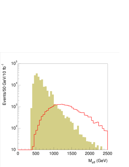
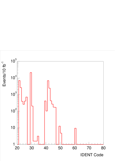
Figure 1: Left: Effective mass distribution for signal (curve) and Standard Model background (shaded). Right: ISAJET IDENT codes for all produced particles contributing to $M_{\rm eff}$ distribution after cuts. The dominant contributions are ${\tilde{q}}_{L}$ (21–26), ${\tilde{g}}$ (29), and ${\tilde{q}}_{R}$ (41–46).

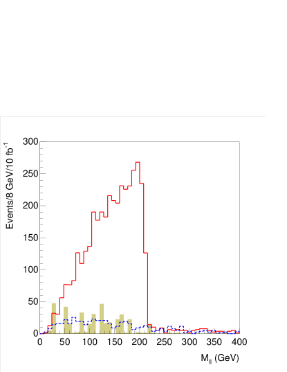
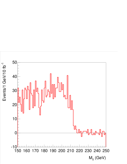
Figure 2: Mass distribution for opposite sign dileptons. Left: Distributions for same flavor signal (solid curve), opposite flavor signal (dashed curve), and Standard Model same flavor background (shaded). Right: $e^{+}e^{-}+\mu^{+}\mu^{-}-e^{\pm}\mu^{\mp}$ distribution for signal on a finer scale.

The mass distribution for $\ell^{+}\ell^{-}$ pairs with the same and opposite flavor is shown in Figure 2. The opposite-flavor distribution is small, and there is a clear endpoint in the same-flavor distribution at

$$M_{\ell\ell}^{\rm max}=\sqrt{(M_{{\tilde{\chi}}_{2}^{0}}^{2}-M_{{\tilde{\ell}}}^{2})(M_{{\tilde{\ell}}}^{2}-M_{\tilde{\chi}_{1}^{0}}^{2})\over M_{{\tilde{\ell}}}^{2}}=213.6,215.3\,{\rm GeV}$$

corresponding to the endpoints for the decays ${\tilde{\chi}}_{2}^{0}\to{\tilde{\ell}}_{L,R}^{\pm}\ell^{\mp}\to{\tilde{\chi}_{1}^{0}}\ell^{+}\ell^{-}$. This is similar to what is seen in SUGRA Point 5, but in that case only one slepton contributes. It is clear from the $e^{+}e^{-}+\mu^{+}\mu^{-}-e^{\pm}\mu^{\mp}$ dilepton distribution with finer bins shown in the same figure that the endpoints for ${\tilde{\ell}}_{R}$ and ${\tilde{\ell}}_{L}$ cannot be resolved with the expected ATLAS dilepton mass resolution. More work is needed to see if the presence of two different endpoints could be inferred from the shape of the edge of the dilepton distribution.

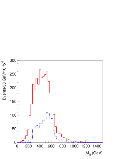
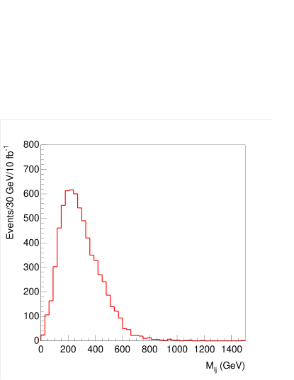
Figure 3: Mass distribution for $e^{+}e^{-}+\mu^{+}\mu^{-}-e^{\pm}\mu^{\mp}$ events combined with one of the two hardest jets. Left: $\ell^{+}\ell^{-}j$ mass distribution (solid) and same with $M_{\ell\ell}>175\,{\rm GeV}$ (dashed). Right: $\ell^{\pm}j$ mass distribution for the one of the two hardest jets that gives the smaller $\ell\ell j$ mass.

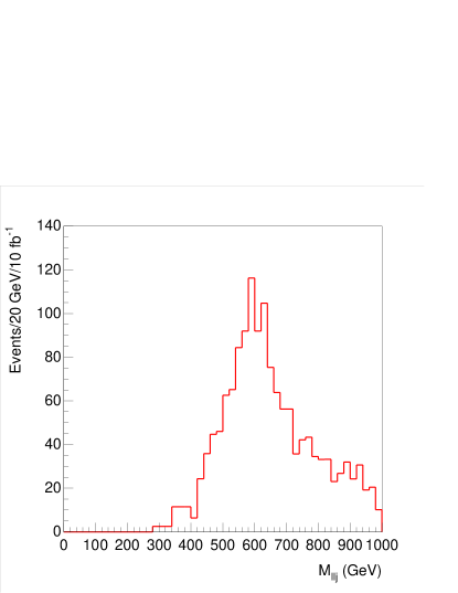
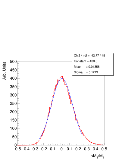
Figure 4: Left: Lower edge from larger $\ell\ell j$ mass combining $e^{+}e^{-}+\mu^{+}\mu^{-}-e^{\pm}\mu^{\mp}$ with one of the two hardest jets. Right: Model-independent fit for ${\tilde{\chi}_{1}^{0}}$ mass.

Since the main source for ${\tilde{\chi}}_{2}^{0}$ is ${\tilde{q}}_{R}\to{\tilde{\chi}}_{2}^{0}q$, information on the squark masses can be obtained by combining the leptons from ${\tilde{\chi}}_{2}^{0}\to{\tilde{\ell}}\ell$ decays with one of the two hardest jets in the event, since the hardest jets are generally products of the squark decays. Figure 3 shows the distribution for the smaller of the two $\ell^{+}\ell^{-}j$ masses formed with the two leptons and each of the two hardest jets in the event. The dashed curve in this figure shows the same distribution for $M_{\ell\ell}>175\,{\rm GeV}$, for which the backgrounds are smaller. Both distributions should have endpoints at the kinematic limit for ${\tilde{q}}_{R}\to{\tilde{\chi}}_{2}^{0}\to{\tilde{\ell}}\ell\to{\tilde{\chi}_{1}^{0}}\ell\ell$,

$$\left[{(M^{2}_{{\tilde{q}}_{R}}-M^{2}_{{\tilde{\chi}}_{2}^{0}})(M^{2}_{{\tilde{\chi}}_{2}^{0}}-M^{2}_{{\tilde{\chi}_{1}^{0}}})\over M^{2}_{{\tilde{\chi}}_{2}^{0}}}\right]^{1/2}=652.9\,{\rm GeV}.$$

Figure 3 also shows the $\ell^{\pm}j$ mass distribution formed with each of the two leptons combined with the jet that gives the smaller of the two $\ell\ell j$ masses. This should have a 3-body endpoint at

$$\left[{(M^{2}_{{\tilde{q}}_{R}}-M^{2}_{{\tilde{\chi}}_{2}^{0}})(M^{2}_{{\tilde{\chi}}_{2}^{0}}-M^{2}_{{\tilde{\ell}}})\over M^{2}_{{\tilde{\chi}}_{2}^{0}}}\right]^{1/2}=605.4\,{\rm GeV}.$$

The branching ratio for ${\tilde{b}}_{1}\to{\tilde{\chi}}_{2}^{0}b$ is very small, so the same distributions with $b$-tagged jets contain only a handful of events and cannot be used to determine the ${\tilde{b}}_{1}$ mass.

The decay chain ${\tilde{q}}_{R}\to{\tilde{\chi}}_{2}^{0}q\to{\tilde{\ell}}_{L,R}^{\pm}\ell^{\mp}q\to{\tilde{\chi}_{1}^{0}}\ell^{+}\ell^{-}q$ also implies a lower limit on the $\ell\ell q$ mass for a given limit on $z=\cos\theta^{*}$ or equivalently on the $\ell\ell$ mass. For $z>0$ (or equivalently $M_{\ell\ell}>M_{\ell\ell}^{\rm max}/\sqrt{2}$) this lower limit is

$$\begin{array}[]{lcl}(M_{\ell\ell q}^{\rm min})^{2}&=&\frac{1}{4M_{2}^{2}M_{e}^{2}}\times\\ &&\Biggl{[}-M_{1}^{2}M_{2}^{4}+3M_{1}^{2}M_{2}^{2}M_{e}^{2}-M_{2}^{4}M_{e}^{2}-M_{2}^{2}M_{e}^{4}-M_{1}^{2}M_{2}^{2}M_{q}^{2}-\\ &&\quad M_{1}^{2}M_{e}^{2}M_{q}^{2}+3M_{2}^{2}M_{e}^{2}M_{q}^{2}-M_{e}^{4}M_{q}^{2}+(M_{2}^{2}-M_{q}^{2})\times\\ &&\quad\sqrt{(M_{1}^{4}+M_{e}^{4})(M_{2}^{2}+M_{e}^{2})^{2}+2M_{1}^{2}M_{e}^{2}(M_{2}^{4}-6M_{2}^{2}M_{e}^{2}+M_{e}^{4})}\Biggr{]}\\ M_{\ell\ell q}^{\rm min}&=&376.6\,{\rm GeV}\end{array}$$

where $M_{q}$, $M_{2}$, $M_{e}$, and $M_{1}$ are the (average) squark, ${\tilde{\chi}}_{2}^{0}$, (average) slepton, and ${\tilde{\chi}_{1}^{0}}$ masses. To determine this lower edge, the larger of the two $\ell\ell j$ masses formed from two opposite-sign leptons and one of the two hardest jets is plotted in Figure 4. An endpoint at about the right value can clearly be seen.

The $\ell^{+}\ell^{-}$, $\ell^{+}\ell^{-}q$, $\ell^{\pm}q$, and lower $\ell^{+}\ell^{-}q$ edges provide four constraints on the four masses involved. Since the cross sections are similar to those for SUGRA Point 5, we take the errors at high luminosity to be negligible on the $\ell^{+}\ell^{-}$ edge, 1% on the $\ell^{+}\ell^{-}q$ and $\ell^{\pm}q$ upper edges, and 2% on the $\ell^{+}\ell^{-}q$ lower edge. Random masses were generated within $\pm 50\%$ of their nominal values, and the $\chi^{2}$ for the four measurements with these errors were used to determine the probability for each set of masses. The resulting distribution for the ${\tilde{\chi}_{1}^{0}}$ mass, also shown in Figure 4, has a width of $\pm 11.7\%$, about the same as for Point 5; the errors for the other masses are also comparable. Of course, the masses being measured in this case are different: for example the squark mass is the average of the ${\tilde{q}}_{R}$ rather than the ${\tilde{q}}_{L}$ masses.

Figure 5: Lepton multiplicity with a hadronic $\tau$ veto. Solid: AMSB model. Dashed: Same but with $M_{1}\leftrightarrow M_{2}$.

The leptons from ${\tilde{\chi}}_{1}^{\pm}\to{\tilde{\chi}_{1}^{0}}\ell^{\pm}\nu$ are very soft. This implies that the rate for events with one or three leptons or for two leptons with opposite flavor are all suppressed. Figure 5 shows as a solid histogram the multiplicity of leptons with $p_{T}>10\,{\rm GeV}$ and $|\eta|<2.5$ for the AMSB signal with a veto on hadronic $\tau$ decays. The same figure shows the distribution for a model with the same weak-scale mass parameters except that the gaugino masses $M_{1}$ and $M_{2}$ are interchanged. This model has a wino ${\tilde{\chi}}_{1}^{\pm}$ approximately degenerate with the ${\tilde{\chi}}_{2}^{0}$ rather than with the ${\tilde{\chi}_{1}^{0}}$. Clearly the AMSB model has a much smaller rate for single leptons and a somewhat smaller rate for three leptons; these rates can be used to distinguish AMSB and SUGRA-like models.

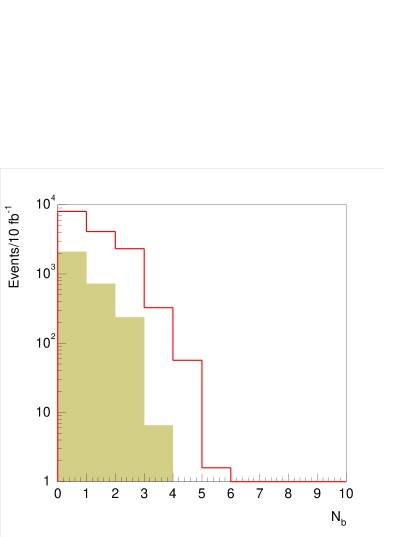
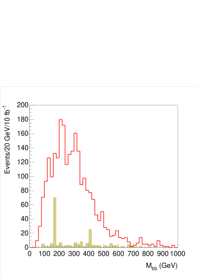
Figure 6: Left: Multiplicity of $b$ jets for signal (curve) and Standard Model background (shaded). Right: Smallest mass for pairs of $b$ jets for signal (curve) and Standard Model background (shaded). Both plots have $M_{\rm eff}>1200\,{\rm GeV}$ in addition to the standard cuts and include a $b$ tagging efficiency $\epsilon_{b}=60\%$.

While the decay ${\tilde{\chi}}_{2}^{0}\to{\tilde{\chi}_{1}^{0}}h$ is kinematically allowed, the branching ratio is only about 0.03%. Other sources of $h$ in SUSY events are also quite small, so in contrast to SUGRA Point 5 there is no strong $h\to b\bar{b}$ signal. However, there is a fairly large branching ratio for ${\tilde{g}}\to{\tilde{b}}\bar{b},{\tilde{t}}\bar{t}$ with ${\tilde{b}}\to{\tilde{\chi}_{1}^{0}}b$, ${\tilde{t}}\to\chi_{1}^{+}b$, giving two hard $b$ jets and hence structure in the $M_{bb}$ distribution. For this analysis $b$ jets were tagged by assuming that any $B$ hadron with $p_{T,B}>10\,{\rm GeV}$ and $|\eta_{B}|<2$ is tagged with an efficiency $\epsilon_{B}=60\%$; the jet with the smallest

$$R=\sqrt{(\Delta\eta)^{2}+(\Delta\phi)^{2}}$$

was then taken to be $b$ jets. The two hardest jets generally come from the squarks. To reconstruct ${\tilde{g}}\to{\tilde{b}}\bar{b}$ one of the two hardest jets, tagged as a $b$, was combined with any remaining jet, also tagged as a $b$. In addition to the standard multijet and $\hbox to0.0pt{\hbox to7.95831pt{\hfil/\hfil}\hss}E_{T}$ cuts, a cut $M_{\rm eff}>1200\,{\rm GeV}$ was made to reduce the Standard Model background. The resulting distributions for the $b$ jet multiplicity and for the smallest $bb$ dijet mass are shown in Figure 6. The dijet mass should have an endpoint at the kinematic limit for ${\tilde{g}}\to{\tilde{b}}_{1}\bar{b}\to{\tilde{\chi}_{1}^{0}}b\bar{b}$,

$$M_{bb}^{\rm max}=\sqrt{(M_{{\tilde{g}}}^{2}-M_{{\tilde{b}}}^{2})(M_{{\tilde{b}}}^{2}-M_{\tilde{\chi}_{1}^{0}}^{2})\over M_{{\tilde{b}}}^{2}}=418.7\,{\rm GeV}.$$

While the figure is roughly consistent with this, the endpoint is not very sharp; more work is needed to assign an error and to understand the high mass tail. There should also be a $b\bar{t}$ endpoint resulting from ${\tilde{g}}\to{\tilde{t}}\bar{t}$, ${\tilde{t}}\to{\tilde{\chi}}_{1}^{+}b$, with $M_{{\tilde{\chi}}_{1}^{+}}\approx M_{\tilde{\chi}_{1}^{0}}$ and essentially invisible. Of course $m_{t}$ has to be kept in the formula. This would be an apparent strong flavor violation in gluino decays and so quite characteristic of these models. Reconstructing the top is more complicated, so this has not yet been studied.

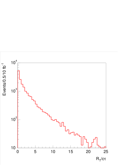
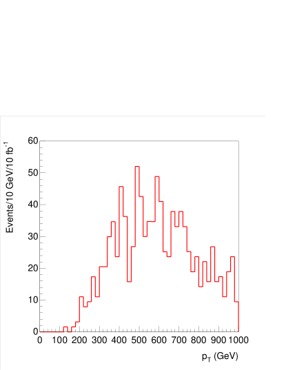
Figure 7: Left: Radial track length distributions for ${\tilde{\chi}}_{1}^{\pm}$ in the barrel region, $|\eta|<1$. Right: $p$ distribution for ${\tilde{\chi}}_{1}^{\pm}$ with $R_{T}>10c\tau$.

The splitting between the ${\tilde{\chi}}_{1}^{\pm}$ and ${\tilde{\chi}_{1}^{0}}$ is very small in AMSB models. ISAJET gives a splitting of $0.189\,{\rm GeV}$ for this point and $c\tau=2.8\,{\rm cm}$, with the dominant decay being the two-body mode ${\tilde{\chi}}_{1}^{\pm}\to{\tilde{\chi}_{1}^{0}}\pi$ via a virtual $W$. Ref.  gives a somewhat smaller value of $\mu$ and so a smaller splitting. The lifetime is of course quite sensitive to the exact splitting. Since the pion or electron is soft and so difficult to reconstruct, it seems better to look for the tail of long-lived winos. The signature is an isolated stiff track in a fraction of the events that ends in the tracking volume and produces no signal in the calorimeter or muon system. Figure 7 shows the radial track length $R_{T}$ distribution in units of $c\tau$ for winos with $|\eta|<1$ and the (generated) momentum distribution for those with $R_{T}>10c\tau$. Note that the ATLAS detector has three layers of pixels with very low occupancy at radii of 4, 11, and 14 cm and four double layers of silicon strips between 30 and 50 cm. It seems likely that the background for tracks that end after the pixel layers would be small.

It is instructive to compare this signature to that for GMSB models with an NLSP slepton. Both models predict long-lived charged particles with $\beta<1$. In the GMSB models, two NLSP sleptons occur in every SUSY event, and they decay into a hard $e$’s, $\mu$’s, or $\tau$’s plus nearly massless ${\tilde{G}}$’s. In the AMSB models, only a fraction of the SUSY events contain long-lived charged tracks, and these decay into a soft pion or electron plus an invisible particle. A detailed tracking simulation should be done for both cases.

Acknowledgement: This work was supported in part by the U.S. Department of Energy under Contract DE-AC02-98CH10886. We also acknowledge the support of the Les Houches Physics Center, where part of this work was done.

References

- [1] L. Randall and R. Sundrum, hep-th/9810155.
- [2] G.F. Giudice, M.A. Luty, H. Murayama and R. Rattazzi, JHEP 12, 027 (1998) hep-ph/9810442.
- [3] T. Gherghetta, G.F. Giudice, and J.D. Wells, hep-ph/9904378.
- [4] J. L. Feng and T. Moroi, hep-ph/9907319.
- [5] H. Baer, F.E. Paige, S.D. Protopescu, X. Tata, hep-ph/9810440.
- [6] I. Hinchliffe, F.E. Paige, M.D. Shapiro, J. Soderqvist, and W. Yao, Phys. Rev. D55, 5520-5540 (1997).
- [7] ATLAS Collaboration, ATLAS Detector and Physics Performance Technical Design Report, CERN/LHCC/99-15.
- [8] J.L. Feng, T. Moroi, L. Randall, M. Strassler and S. Su, Phys. Rev. Lett. 83, 1731 (1999) hep-ph/9904250.
- [9] A. Pomarol and R. Rattazzi, JHEP 05, 013 (1999) hep-ph/9903448.
- [10] R. Rattazzi, A. Strumia, J.D. Wells, hep-ph/9912390.