Abstract

Properties of mesons are investigated within the Nambu–Jona-Lasinio model. We include meson-loop corrections, which are generated via a systematic $1/N_{c}$-expansion in next-to-leading order. We show that our scheme is consistent with chiral symmetry, in particular with the Goldstone theorem and the Gell-Mann Oakes Renner relation. The numerical part focuses on the pion and the $\rho$-meson sector. For the latter the $1/N_{c}$-corrections are crucial in order to include the dominant $\rho\rightarrow\pi\pi$-decay channel, while the leading-order approximation only contains unphysical $q\bar{q}$-decay channels. We show that a satisfactory description of the pion electromagnetic form factor can be obtained. Similarities and differences to hadronic models are discussed.

1 Introduction

The understanding of hadron properties in the vacuum as well as in hot or dense matter is one of the central tasks of present-day nuclear physics. In principle, all properties of strongly interacting particles should be derived from QCD. However, at least in the low-energy regime, where perturbation theory is not applicable, this is presently limited to a rather small number of observables which can be studied on the lattice, while more complex processes have to be described within model calculations.

So far the best descriptions of hadronic spectra, decays and scattering processes are obtained within phenomenological hadronic models. For instance the pion electromagnetic form factor in the time-like region can be reproduced rather well within a simple vector dominance model with a dressed $\rho$-meson which is constructed by coupling a bare $\rho$-meson to a two-pion intermediate state [1, 2]. Models of this type have been successfully extended to investigate medium modifications of vector mesons and to calculate dilepton production rates in hot and dense hadronic matter [3].

In this situation one might ask how the phenomenologially successful hadronic models emerge from the underlying quark structure and the symmetry properties of QCD. Since this question cannot be answered at present from first principles it has to be addressed within quark models. For light hadrons chiral symmetry and its spontaneous breaking in the physical vacuum through instantons plays the decisive role in describing the two-point correlators [4] with confinement being much less important. This feature is captured by the Nambu–Jona-Lasinio(NJL) model in which the four-fermion interactions can be viewed as being induced by instantons.

The study of hadrons within the NJL model has of course a long history. In fact, mesons of various quantum numbers have already been discussed in the original papers by Nambu and Jona-Lasinio [5] and by many authors thereafter (for reviews see [6, 7, 8]). Most of these works correspond to a leading-order approximation in $1/N_{c}$, the inverse number of colors. In this scheme quark masses are calculated in mean-field approximation and mesons are constructed as correlated quark-antiquark states. With the appropriate choice of parameters chiral symmetry, which is an (approximate) symmetry of the model Lagrangian, is spontaneously broken in the vacuum and pions emerge as (nearly) massless Goldstone bosons. While this is clearly one of the successes of the model, the description of other mesons is more problematic. One reason is the fact that the NJL model does not confine quarks. As a consequence a meson can decay into free constituent quarks if its mass is larger than twice the constituent quark mass $m$. Hence, for a typical value of $m\sim$ 300 MeV, the $\rho$-meson with a mass of 770 MeV, for instance, would be unstable against decay into quarks. On the other hand the physical decay channel of the $\rho$-meson into two pions is not included in the standard approximation. Hence, even if a large constituent quark mass is chosen in order to suppress the unphysical decays into quarks, one obtains a poor description of the $\rho$-meson propagator and related observables, like the pion electromagnetic form factor.

This and other reasons have motivated several authors to go beyond the standard approximation scheme and to include mesonic fluctuations. In Ref. [9] a quark-antiquark $\rho$-meson is coupled via a quark triangle to a two-pion state. Also higher-order corrections to the quark self-energy [10] and to the quark condensate [11] have been investigated. However, as the most important feature of the NJL model is chiral symmetry, one should use an approximation scheme which conserves the symmetry properties, to ensure the existence of massless Goldstone bosons.

Two slightly different symmetry conserving approximation schemes are discussed in Refs. [12] and [13]. The authors of Ref. [13] use an expansion in $1/N_{c}$ in order to include mesonic fluctuations and calculate the changes of $f_{\pi}$ and of the quark condensate $\langle{\bar{\psi}\psi}\rangle$ in a low-momentum expansion for the incoming state. In Ref. [12] a correction term to the quark self-energy is included in the gap equation. In a perturbative scheme this term would be of order $1/N_{c}$ but, as the modified gap equation is solved self-consistently, arbitrary orders in $1/N_{c}$ are generated. The authors find a consistent scheme to describe mesons and show the validity of the Goldstone theorem and the Goldberger-Treiman relation in that scheme. Based on this model various authors have investigated the effect of meson-loop corrections on the pion electromagnetic form factor [14] and on $\pi$-$\pi$ scattering in the vector [15] and the scalar channel [16]. However, since the numerical calculation of the multi-loop diagrams, which have to be evaluated, is rather involved, in these references the exact expressions are approximated by low-momentum expansions.

In the present paper we calculate the $\rho$-meson self energy in a strict expansion up to next-to-leading order without any approximations. Within the same scheme we have recently studied the influence of mesonic fluctuations on the pion propagator [17]. This was mainly motivated by recent works by Kleinert and Van den Bossche [18], who claim that chiral symmetry is not spontaneously broken in the NJL model as a result of strong mesonic fluctuations. In Ref. [17] we argue that because of the non-renormalizability of the NJL model new divergences and hence new cutoff parameters emerge if one includes meson loops. Following Refs. [12] and [13] we regularize the meson loops by an independent cutoff parameter $\Lambda_{M}$. The results are, of course, strongly dependent on this parameter. Whereas for moderate values of $\Lambda_{M}$ the pion properties change only quantitatively strong instabilities are encountered for larger values of $\Lambda_{M}$, which might be a hint for an instability of the spontaneously broken vacuum state.

In Ref. [17] we restricted ourselves to calculate the pion mass $m_{\pi}$, the pion decay constant $f_{\pi}$ and the quark condensate $\langle{\bar{\psi}\psi}\rangle$. Since these quantities can already be fitted without meson-loop corrections (i.e. $\Lambda_{M}$ = 0) one has to look at other observables in order to fix $\Lambda_{M}$. Obviously the spectral function of the $\rho$-meson is particularly suited, as it cannot be described realistically without taking into account pion loops. In the present article all parameters of the NJL model will be fixed by fitting $\rho$-meson properties simultaneously with $f_{\pi}$ and $\langle{\bar{\psi}\psi}\rangle$. The important result is that such a fit can indeed be achieved with a constituent quark mass which is large enough such that the unphysical $q\bar{q}$-threshold opens above the $\rho$-meson peak. Since the constituent quark mass is not an independent input parameter this was not clear a priori.

The paper is organized as follows. In Sec. 2 we present the scheme for describing mesons in next-to-leading order in $1/N_{c}$. The consistency of this scheme with the Goldstone theorem and with the Gell-Mann Oakes Renner relation will be shown in Sec. 3. In Sec. 4 we perform a low-momentum expansion of the effective meson vertices and discuss the relation to hadronic models. The numerical results will be presented in Sec. 5. For several values of $\Lambda_{M}$ we fix a subset of the model parameters by fitting quantities in the pion sector. Then we determine the remaining parameters, in particular $\Lambda_{M}$, in the $\rho$-meson sector. Finally, conclusions are drawn in Sec. 6.

2 The NJL model in leading order and next-to-leading order in $1/N_{c}$

We consider the following NJL-type Lagrangian:

$${\cal L}\;=\;\bar{\psi}(i\partial{\hskip-5.69054pt}/-m_{0})\psi\;+\;g_{s}\,[(\bar{\psi}\psi)^{2}+(\bar{\psi}i\gamma_{5}{\vec{\tau}}\psi)^{2}]\;-\;g_{v}\,[(\bar{\psi}\gamma^{\mu}{\vec{\tau}}\psi)^{2}+(\bar{\psi}\gamma^{\mu}\gamma_{5}{\vec{\tau}}\psi)^{2}]\,.$$ (1)

Here $\psi$ is a quark field with $N_{f}$ = 2 flavors and $N_{c}$ colors, while $g_{s}$ and $g_{v}$ are dimensionful coupling constants of the order $1/N_{c}$. In order to establish the counting scheme, the number of colors has been treated as variable, but all numerical calculations will be done with the physical value, $N_{c}$ = 3.

In most publications the NJL model has been treated in leading order in $1/N_{c}$. In terms of many-body theory this corresponds to a (Bogoliubov) Hartree approximation for the quark propagator and to a random phase approximation (RPA) for describing mesonic excitations. Diagrammatically this is shown in Fig. 1. The selfconsistent solution of the Dyson equation shown in the upper part of Fig. 1 leads to a momentum independent quark self energy and therefore only gives a correction to the constituent quark mass:

$$m\;=\;m_{0}\;+\;2ig_{s}\ 4N_{c}N_{f}\int\frac{d^{4}p}{(2\pi)^{4}}{m\over{p^{2}-m^{2}+i\epsilon}}~{}.$$ (2)

Usually one refers to this equation as the gap equation. For sufficiently large couplings $g_{s}$ it allows for a finite constituent quark mass $m$ even in the chiral limit, i.e. for $m_{0}$ = 0. In the mean-field approximation this solution minimizes the ground-state energy. Since $g_{s}$ is of order $1/N_{c}$ the constituent quark mass $m$, and hence the quark propagator $S(p)=(p/-m)^{-1}$ are of the order unity.

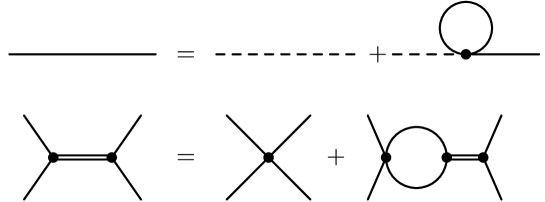
Figure 1: (Upper part) The Dyson equation for the quark propagator in the Hartree approximation (solid lines). The dashed lines denote the bare quark propagator. (Lower part) The Bethe-Salpeter equation for the meson propagator in the RPA (double line). Again, the single solid lines indicate quark propagators in the Hartree approximation.

Mesons are described via a Bethe-Salpeter equation, as shown in the lower part of Fig. 1. Since this is all standard we only list the results, which are needed later on. First we define the quark-antiquark polarization functions

$$\Pi_{M}(q)\;=\;-i\int\frac{d^{4}p}{(2\pi)^{4}}{\rm Tr}[\,\Gamma_{M}\,iS(p+{q\over 2})\,\Gamma_{M}\,iS(p-{q\over 2})\,]\;,$$ (3)

with $M=\sigma,\pi,\rho,a_{1}$ and $\Gamma_{\sigma}=1\!\!1$, $\Gamma_{\pi}^{k}=i\gamma_{5}\tau^{k}$, $\Gamma_{\rho}^{\mu\,k}=\gamma^{\mu}\tau^{k}$ and $\Gamma_{a_{1}}^{\mu\,k}=\gamma^{\mu}\gamma_{5}\tau^{k}$. Here “${\rm Tr}$” denotes a trace in color, flavor and Dirac space. $\Pi_{M}$ is diagrammatically shown in Fig. 3. Iterating the scalar (pseudoscalar) part of the four-fermion interaction one obtains for the sigma meson (pion):

$$D_{\sigma}(q)\;=\;\frac{-2g_{s}}{1-2g_{s}\Pi_{\sigma}(q)}\;,\qquad D_{\pi}^{ab}(q)\;\equiv\;D_{\pi}(q)\,\delta_{ab}\;=\;\frac{-2g_{s}}{1-2g_{s}\Pi_{\pi}(q)}\,\delta_{ab}\;.$$ (4)

Here $a$ and $b$ are isospin indices and we have used the notation $\Pi_{\pi}^{ab}(q)\equiv\Pi_{\pi}(q)\,\delta_{ab}$.

In the vector channel this can be done in a similar way. Using the transverse structure of the polarization loop in the vector channel,

$$\Pi_{\rho}^{\mu\nu,ab}(q)\;=\;\Pi_{\rho}(q)\,T^{\mu\nu}\,\delta_{ab}\;;\qquad T^{\mu\nu}=(-g^{\mu\nu}+\frac{q^{\mu}q^{\nu}}{q^{2}})\;,$$ (5)

one obtains for the $\rho$-meson

$$D_{\rho}^{\mu\nu,ab}(q)\;\equiv\;D_{\rho}(q)\;T^{\mu\nu}\;\delta_{ab}\;=\;\frac{-2g_{v}}{1-2g_{v}\Pi_{\rho}(q)}\,T^{\mu\nu}\;\delta_{ab}\;.$$ (6)

Analogously, the $a_{1}$ can be constructed from the transverse part of the axial polarization function $\Pi_{a_{1}}$. As discussed e.g. in Ref. [19] $\Pi_{a_{1}}^{\mu\nu}$ also contains a longitudinal part which contributes to the pion. Although there is no conceptional problem to include this mixing we will neglect it in the present paper in order to keep the structure of the model as simple as possible.

It follows from Eqs. (3) - (6) that the functions $D_{M}(q)$ are of order $1/N_{c}$. Their explicit forms are given in App. B. For simplicity we will call them “propagators”, although strictly speaking, they should be interpreted as the product of a renormalized meson propagator with a squared quark-meson coupling constant. The latter is given by the inverse residue of the function $D_{M}(q)$, while the pole position determines the meson mass:

$$D_{M}^{-1}(q)|_{q^{2}=m_{M}^{2(0)}}\;=\;0\;,\qquad g_{Mqq}^{-2(0)}\;=\;\frac{d\Pi_{M}(q)}{dq^{2}}|_{q^{2}=m_{M}^{2(0)}}\;.$$ (7)

We have used the superscript $(0)$ to indicate that $m_{M}^{2(0)}$ and $g_{Mqq}^{-2(0)}$ are leading-order quantities in $1/N_{c}$. One easily verifies that they are of order unity and $1/\sqrt{N_{c}}$, respectively. With the help of the gap equation, Eq. (2), one can show that the pion is massless in the chiral limit, demonstrating the consistency of the scheme with chiral symmetry [5].

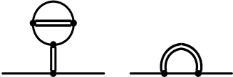
Figure 2: The $1/N_{c}$-corrections to the quark self-energy.

We now turn to the corrections in next-to-leading order in $1/N_{c}$. The correction terms to the quark self-energy are shown in Fig. 2. In these diagrams the quark lines and the double lines correspond to quark propagators in the Hartree approximation (order unity) and to meson propagators in the RPA (order $1/N_{c}$), respectively. Both diagrams are therefore of order $1/N_{c}$.

The $1/N_{c}$-corrected mesonic polarization diagrams read

$${\tilde{\Pi}}_{M}(q)\;=\;\Pi_{M}(q)\;+\;\sum_{k=a,b,c,d}\;\delta\Pi_{M}^{(k)}(q)\;.$$ (8)

The four correction terms $\delta\Pi_{M}^{(a)}$ - $\delta\Pi_{M}^{(d)}$ together with the leading-order term $\Pi_{M}$ are shown in Fig. 3. Again the lines in this figure correspond to Hartree quarks and RPA mesons. Besides the RPA meson propagators the main building blocks are quark triangle and box diagrams, which are shown in Fig. 4. The triangle diagrams entering into $\delta\Pi_{M}^{(a)}$ and $\delta\Pi_{M}^{(d)}$ can be interpreted as effective three-meson vertices. For external mesons $M_{1}$, $M_{2}$ and $M_{3}$ they are given by

$$-i\Gamma_{M_{1},M_{2},M_{3}}(q,p) = -\int\frac{d^{4}k}{(2\pi)^{4}}\Big{\{}{\rm Tr}[\Gamma_{M_{1}}iS(k)\Gamma_{M_{2}}iS(k-p)\Gamma_{M_{3}}iS(k+q)]$$ (9)

$$\hskip 51.21504pt+{\rm Tr}[\Gamma_{M_{1}}iS(k-q)\Gamma_{M_{3}}iS(k+p)\Gamma_{M_{2}}iS(k)]\Big{\}}~{},$$

with the operators $\Gamma_{M}$ as defined below Eq. (3). We have summed over both possible orientations of the quark loop.

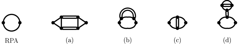
Figure 3: Contributions to the mesonic polarization function in leading (RPA) and next-to-leading order in $1/N_{c}$.

The quark box diagrams are effective four-meson vertices and are needed for the evaluation of $\delta\Pi_{M}^{(b)}$ and $\delta\Pi_{M}^{(c)}$. If one again sums over both orientations of the quark loop they are given by

$$-i\Gamma_{M_{1},M_{2},M_{3},M_{4}}(p_{1},p_{2},p_{3})\phantom{\int\frac{d^{4}k}{(2\pi)^{4}}}$$ (10)

$$= \int\frac{d^{4}k}{(2\pi)^{4}}\Big{(}{\rm Tr}[\Gamma_{M_{1}}iS(k)\Gamma_{M_{2}}iS(k-p_{2})\Gamma_{M_{3}}iS(k-p_{2}-p_{3})\Gamma_{M_{4}}iS(k+p_{1})]$$

$$\hskip 36.98866pt+{\rm Tr}[\Gamma_{M_{1}}iS(k-p_{1})\Gamma_{M_{4}}iS(k+p_{2}+p_{3})\Gamma_{M_{3}}iS(k+p_{2})\Gamma_{M_{2}}iS(k)]\Big{)}~{}.$$

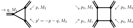
Figure 4: (Left) The quark triangle vertex $-i\Gamma_{M_{1},M_{2},M_{3}}(q,p)$. (Right) The quark box vertex $-i\Gamma_{M_{1},M_{2},M_{3},M_{4}}(p_{1},p_{2},p_{3})$.

The polarization diagrams $\delta\Pi_{M}^{(a)}$ - $\delta\Pi_{M}^{(d)}$ contain several loops. However, with the help of the definitions given above they can be written in a relatively compact form:

$$\delta\Pi^{(a)}_{M}(q) \;=\; \phantom{-}\frac{i}{2}\int\frac{d^{4}p}{(2\pi)^{4}}\sum_{M_{1}M_{2}}\Gamma_{M,M_{1},M_{2}}(q,p)\,D_{M_{1}}(p)\,\Gamma_{M,M_{1},M_{2}}(-q,-p)\,D_{M_{2}}(-p-q)\;,$$

$$\delta\Pi^{(b)}_{M}(q) \;=\; -i\,\int\frac{d^{4}p}{(2\pi)^{4}}\hskip 8.53581pt\sum_{M_{1}}\;\Gamma_{M,M_{1},M_{1},M}(q,p,-p)\,D_{M_{1}}(p)\;,$$

$$\delta\Pi^{(c)}_{M}(q) \;=\; -\frac{i}{2}\int\frac{d^{4}p}{(2\pi)^{4}}\hskip 7.11317pt\sum_{M_{1}}\;\Gamma_{M,M_{1},M,M_{1}}(q,p,-q)\,D_{M_{1}}(p)\;,$$

$$\delta\Pi^{(d)}_{M}(q) \;=\; \frac{i}{2}\;\Gamma_{M,M,\sigma}(q,-q)\,D_{\sigma}(0)\;\int\frac{d^{4}p}{(2\pi)^{4}}\hskip 8.53581pt\sum_{M_{1}}\;\Gamma_{M_{1},M_{1},\sigma}(p,-p)\,D_{M_{1}}(p)\;.$$ (11)

Note that for $\delta\Pi^{(c)}_{M}$ and $\delta\Pi^{(d)}_{M}$ one has to include a symmetry factor of $1/2$, because otherwise the sum over the two orientations of the quark propagators, which is contained in the definitions of the quark triangle vertex (Eq. (9)) and of the quark box vertex (Eq. (10)) would lead to double counting. Similarly in $\delta\Pi^{(a)}_{M}$ we had to correct for the fact that the exchange of $M_{1}$ and $M_{2}$ leads to identical diagrams.

For the evaluation of Eq. (11) we have to proceed in two steps. In the first step we calculate the intermediate RPA meson-propagators. Simultaneously we can calculate the quark triangles and box diagrams. One is then left with a meson loop which has to be evaluated in a second step.

The various sums are, in principle, over all quantum numbers of the intermediate mesons. Of course, many combinations vanish, e.g. because of isospin conservation. In fact, the expression for $\delta\Pi^{(d)}_{M}(q)$ should contain a sum over the quantum numbers of both intermediate mesons. However, one can easily verify that the meson which connects the two quark triangles has to be a sigma meson in order to give a non-vanishing contribution.

As we have mentioned earlier, the main focus of the present paper is on the $\rho$-meson. In this case the most important contribution comes from the two-pion intermediate state in diagram $\delta\Pi^{(a)}_{M}$. Other contributions to this diagram, i.e $\pi a_{1}$, $\rho\sigma$, $\rho\rho$ and $a_{1}a_{1}$ intermediate states, are much less important since the corresponding decay channels open far above the $\rho$-meson mass and - in the NJL model - also above the unphysical two-quark threshold. Hence, from a purely phenomenological point of view, it should be sufficient to restrict the sums in Eq. (11) to intermediate pions. However, in order to stay consistent with chiral symmetry, we have to include intermediate sigma mesons as well. On the other hand, vector- and axial-vector mesons can be neglected without violating chiral symmetry. Since this leads to an appreciable simplification of the numerics we have restricted the intermediate degrees of freedom to scalar and pseudoscalar mesons in the present paper. Of course, in order to describe a $\rho$-meson, we have to take vector couplings at the external vertices of the diagrams shown in Fig. 3.

In analogy to Eqs. (4) and (6) the corrected meson propagators are given by

$${\tilde{D}}_{M}(q)\;=\;\frac{-2g_{M}}{1-2g_{M}{\tilde{\Pi}}_{M}(q)}\;,$$ (12)

with $g_{M}=g_{s}$ for $\sigma$ and $\pi$ and $g_{M}=g_{v}$ for $\rho$ and $a_{1}$. Since our scheme corresponds to a $1/N_{c}$-expansion of the polarization diagrams and hence of the inverse meson propagators, the ${\tilde{D}}_{M}$ contains terms of arbitrary orders in $1/N_{c}$.

The corrected meson masses are again defined by the pole positions of the propagators:

$$\tilde{D}_{M}^{-1}(q)|_{q^{2}=m_{M}^{2}}\;=\;0\;.$$ (13)

As we will show in the next section our scheme is consistent with the Goldstone theorem, i.e. in the chiral limit it leads to massless pions. Note, however, that because of its implicit definition $m_{M}$ contains terms of arbitrary orders in $1/N_{c}$, although we start from a strict expansion of the inverse meson propagator up to next-to-leading order. This will be important in the context of the Gell-Mann Oakes Renner relation.

Finally we should comment on Ref. [12], where the authors introduce $1/N_{c}$-corrections in a slightly different way. In that scheme a correction term to the quark self-energy is self-consistently included in the gap equation. This leads to a modified quark mass as compared to the ’Hartree mass’. Mesons are described by iterating the polarization diagrams $\Pi_{M}$, $\delta\Pi_{M}^{(a)}$, $\delta\Pi_{M}^{(b)}$ and $\delta\Pi_{M}^{(c)}$, but using the modified quarks for constructing RPA mesons as well as quark triangle- and box diagrams. Since the $1/N_{c}$-correction terms are iterated in the gap equation, all diagrams contain terms of arbitrary orders in $1/N_{c}$. However, if one performs a strict $1/N_{c}$-expansion of the mesonic polarization diagrams one exactly recovers our scheme of describing mesons [12].

Both schemes, the one introduced in Ref. [12] and the strict $1/N_{c}$-expansion, are consistent with chiral symmetry. In particular, they lead to massless pions in the chiral limit. However, because of the modified gap equation, in the scheme of Ref. [12] the RPA pions are not massless in the chiral limit, but tachyonic. Therefore this model is not very well suited for calculating the $\rho$-meson self-energy, which is mainly determined by intermediate RPA pions. For this reason we prefer the strict $1/N_{c}$-expansion scheme, in which both RPA- and $1/N_{c}$-corrected pions are massless in the chiral limit. Still there remains the problem that $m_{\pi}\neq m_{\pi}^{(0)}$, if we go away from the chiral limit, but at least for our final parameter set the difference is only about 10%. This will be discussed in more detail in Sec. 5.

3 Consistency with chiral symmetry

Before discussing the numerical details we wish to show that the scheme introduced in the previous section is consistent with chiral symmetry. We begin with the Goldstone theorem and then show the consistency of the scheme with the Gell-Mann Oakes Renner relation. This is not an entirely academic exercise. Since most of the integrals which have to be evaluated are divergent and hence must be regularized one has to ensure that the various symmetry relations are not destroyed by the regularization. To this end, it is important to know how these relations formally emerge.

The validity of the Goldstone theorem in our scheme has already been proven by Dmitrašinović et al. [12] and we only summarize the main steps which are relevant for our later discussion. One has to show that, in the chiral limit, the inverse pion propagator vanishes at zero momentum,

$$2g_{s}\,{\tilde{\Pi}}_{\pi}(0)\;=\;1\qquad{\rm for}\quad m_{0}\;=\;0.$$ (14)

As before we use the notation ${\tilde{\Pi}}^{ab}_{\pi}=\delta_{ab}{\tilde{\Pi}}_{\pi}$. Restricting the calculation to the chiral limit and to zero momentum simplifies the expressions considerably and Eq. (14) can be proven analytically. Since the Goldstone theorem is fulfilled in leading order, i.e. $2g_{s}\,\Pi_{\pi}(0)$ = 1 for $m_{0}$ = 0, we only need to show that the contributions of the correction terms add up to zero:

$$\sum_{k=a,b,c,d}\;\delta\Pi_{\pi}^{(k)}(0)\;=\;0\qquad{\rm for}\quad m_{0}\;=\;0.$$ (15)

Let us begin with diagram $\delta\Pi_{\pi}^{(a)}$. As mentioned above, we neglect the $\rho$ and $a_{1}$ subspace for intermediate mesons. Then one can easily see that the external pion can only couple to a $\pi\sigma$ intermediate state. Evaluating the trace in Eq. (9) for zero external momentum one gets for the corresponding triangle diagram:

$$\Gamma_{\pi,\pi,\sigma}^{ab}(0,p)=-\delta_{ab}\ 4N_{c}N_{f}\ 2m\ I(p)~{},$$ (16)

with $a$ and $b$ being isospin indices and the elementary integral

$$I(p)=\int\frac{d^{4}k}{(2\pi)^{4}}\frac{1}{(k^{2}-m^{2}+i\varepsilon)((k+p)^{2}-m^{2}+i\varepsilon)}\;.$$ (17)

Inserting this into Eq. (11) we find

$$\delta\Pi_{\pi}^{(a)\,ab}(0)\;=\;i\delta_{ab}\int\frac{d^{4}p}{(2\pi)^{4}}(4N_{c}N_{f}I(p))^{2}4m^{2}\ D_{\sigma}(p)\ D_{\pi}(p)\;.$$ (18)

Now the essential step is to realize that the product of the RPA sigma- and pion propagators can be converted into a difference [12],

$$D_{\sigma}(p)\ D_{\pi}(p)=i\,\frac{D_{\sigma}(p)-D_{\pi}(p)}{4N_{c}N_{f}\ 2m^{2}\ I(p)}\;,$$ (19)

to finally obtain

$$\delta\Pi_{\pi}^{(a)\,ab}(0)=-\delta_{ab}\;4N_{c}N_{f}\int\frac{d^{4}p}{(2\pi)^{4}}2I(p)\Big{\{}D_{\sigma}(p)-D_{\pi}(p)\Big{\}}\;.$$ (20)

The next two diagrams can be evaluated straightforwardly. One finds:

$$\delta\Pi_{\pi}^{(b)\,ab}(0) = -\delta_{ab}\;4N_{c}N_{f}\int\frac{d^{4}p}{(2\pi)^{4}}\Big{\{}D_{\sigma}(p)\ \big{(}I(p)+I(0)-(p^{2}-4m^{2})\ K(p)\big{)}$$

$$\hskip 99.58464pt+D_{\pi}(p)\ \big{(}3I(p)\hskip 5.69046pt+\;3I(0)\hskip 11.38092pt-\;\;3p^{2}\ K(p)\big{)}\;\Big{\}}\;,$$

$$\delta\Pi_{\pi}^{(c)\,ab}(0) = -\delta_{ab}\;4N_{c}N_{f}\int\frac{d^{4}p}{(2\pi)^{4}}I(p)\Big{\{}-D_{\sigma}(p)-D_{\pi}(p)\Big{\}}\;.$$ (21)

The elementary integral $K(p)$ is of the same type as the integral $I(p)$ and is defined in App. A. Finally we have to calculate $\delta\Pi_{\pi}^{(d)}(0)$. According to Eq. (11), it can be written in the form

$$\delta\Pi_{\pi}^{(d)\,ab}(0)\;=\;-i\Gamma^{ab}_{\pi,\pi,\sigma}(0,0)\,D_{\sigma}(0)\,\Delta\;,$$ (22)

with

$$\Delta = \frac{1}{2}\int\frac{d^{4}p}{(2\pi)^{4}}\sum_{M}(-iD_{M}(p))(-i\Gamma_{M,M,\sigma}(p,-p))$$ (23)

$$= 4N_{c}N_{f}\ m\int\frac{d^{4}p}{(2\pi)^{4}}{\Big{\{}}\ D_{\sigma}(p)\ (2\ I(p)+I(0)-(p^{2}-4m^{2})\ K(p))$$

$$\hskip 93.89418pt+D_{\pi}(p)\ (\;3I(0)\;-\;3p^{2}\ K(p)\;)\hskip 71.13188pt{\Big{\}}}~{}.$$

Evaluating $D_{\sigma}(0)$ in the chiral limit and comparing the result with Eq. (16) one finds that the product of the first two factors in Eq. (22) is simply $\delta_{ab}/m$, i.e. one gets

$$\delta\Pi_{\pi}^{(d)\,ab}(0)=\delta_{ab}\,\frac{\Delta}{m}~{}.$$ (24)

With these results one can easily check that Eq. (15) indeed holds in our scheme.

Of course, most of the integrals we have to deal with are divergent and have to be regularized. Therefore one has to make sure that all steps which lead to Eq. (15) remain valid in the regularized model. One important observation is that the cancellations occur already on the level of the $p$-integrand, i.e. before performing the meson-loop integral. This means that there is no restriction on the regularization of this loop. We also do not need to perform the various quark loop integrals explicitly but can make use of several relations between them. For instance, in order to arrive at Eq. (24) we need the similar structure of quark triangle $\Gamma_{\pi,\pi,\sigma}(0,0)$ and the inverse RPA propagator $D_{\sigma}(0)^{-1}$. Therefore all quark loops, i.e. RPA polarizations, triangles and box diagrams should be consistently regularized within the same scheme, whereas the meson loops can be regularized independently.

Going away from the chiral limit the pion gets a finite mass. To lowest order in the current quark mass it is given by the Gell-Mann Oakes Renner (GOR) relation,

$$m_{\pi}^{2}\,f_{\pi}^{2}\;=\;-m_{0}\,\langle{\bar{\psi}\psi}\rangle\;.$$ (25)

Our scheme is consistent with this relation up to next-to-leading order in $1/N_{c}$. Expanding both sides of Eq. (25) we get

$$m_{\pi}^{2(0)}f_{\pi}^{2(0)}\;+\;m_{\pi}^{2(0)}\delta f_{\pi}^{2}\;+\;\delta m_{\pi}^{2}f_{\pi}^{2(0)}=-m_{0}\,\Big{(}\langle{\bar{\psi}\psi}\rangle^{(0)}+\delta\langle{\bar{\psi}\psi}\rangle\Big{)}\;.$$ (26)

Here $m_{\pi}^{2(0)}$ denotes the leading-order contribution to the squared pion mass, while $\delta m_{\pi}^{2}$ is the next-to-leading order contribution. For $f_{\pi}^{2}$ and $\langle{\bar{\psi}\psi}\rangle$ we introduce similar notations. Since the GOR relation holds only in lowest order in $m_{0}$, Eq. (26) corresponds to a double expansion: $m_{\pi}^{2}$ has to be calculated in linear order in $m_{0}$, $f_{\pi}^{2}$ and $\langle{\bar{\psi}\psi}\rangle$ in the chiral limit.

The quark condensate is given by

$$\langle{\bar{\psi}\psi}\rangle\;=\;-i\int\frac{d^{4}p}{(2\pi)^{4}}Tr{\tilde{S}}(p)\;,$$ (27)

with the $1/N_{c}$-corrected quark propagator

$${\tilde{S}}(p)\;=\;S(p)\;+\;S(p)\,(\Sigma^{(a)}\;+\;\Sigma^{(b)}(p))\,S(p)\;.$$ (28)

Here $S(p)$ is the Hartree propagator and $\Sigma^{(a)}$ and $\Sigma^{(b)}$ are the self energy corrections shown in Fig. 2. Since we are interested in a strict $1/N_{c}$ expansion, it should not be iterated. The r.h.s. of Eq. (27) can be easily evaluated and one obtains

$$\langle{\bar{\psi}\psi}\rangle^{(0)}+\delta\langle{\bar{\psi}\psi}\rangle\;=\;-\frac{m-m_{0}}{2g_{s}}\;-\;\frac{D_{\sigma}(0)\,\Delta}{2g_{s}}\;,$$ (29)

with $\Delta$ as defined in Eq. (23).

The pion decay constant $f_{\pi}$ is calculated from the one-pion to vacuum axial vector matrix element. Basically this corresponds to evaluating the mesonic polarization diagrams, Fig. 3, coupled to an external axial current and to a pion. This leads to expressions similar to Eqs. (3) and (11), but with one external vertex equal to $\gamma^{\mu}\gamma_{5}\frac{\tau^{a}}{2}$, corresponding to the axial current, and the second external vertex equal to $g_{\pi qq}i\gamma_{5}\tau^{b}$, corresponding to the pion. Here the $1/N_{c}$-corrected pion-quark coupling constant is defined as

$$g_{\pi qq}^{-2}\;=\;g_{\pi qq}^{-2(0)}\;+\;\delta g_{\pi qq}^{-2}\;=\;\frac{d{\tilde{\Pi}}_{\pi}(q)}{dq^{2}}|_{q^{2}=m_{\pi}^{2}}\;,$$ (30)

analogously to Eq. (7). Now we take the divergence of the axial current and then use the axial Ward identity

$$\gamma_{5}\,p\!\!\!/\;=\;2m\gamma_{5}\,+\gamma_{5}\,S^{-1}(k+p)\,+S^{-1}(k)\,\gamma_{5}$$ (31)

to simplify the expressions [12]. One finds:

$$f_{\pi}\;=\;g_{\pi qq}\;\Big{(}\;\frac{{\tilde{\Pi}}_{\pi}(q)-{\tilde{\Pi}}_{\pi}(0)}{q^{2}}\,m\;+\;\frac{\Pi_{\pi}(q)-\Pi_{\pi}(0)}{q^{2}}\,D_{\sigma}(0)\,\Delta\;\Big{)}\Big{|}_{q^{2}=m_{\pi}^{2}}\;.$$ (32)

In the chiral limit, $q^{2}=m_{\pi}^{2}\rightarrow 0$, Eqs. (7) and (30) can be employed to replace the difference ratios on the r.h.s. by pion-quark coupling constants. When we square this result and only keep the leading order and the next-to-leading order in $1/N_{c}$ to finally obtain:

$$f_{\pi}^{2(0)}\;+\;\delta f_{\pi}^{2}\;=\;m^{2}\,g_{\pi qq}^{-2(0)}\;+\;\Big{(}\,m^{2}\,\delta g_{\pi qq}^{-2}\;+\;2m\,D_{\sigma}(0)\,\Delta\,g_{\pi qq}^{-2(0)}\,\Big{)}~{}.$$ (33)

For the pion mass we start from Eqs. (12) and (13) and expand the inverse pion propagator around $q^{2}=0$:

$$1\;-\;2g_{s}\,{\tilde{\Pi}}_{\pi}(0)\;-\;2g_{s}\,\Big{(}\frac{d}{dq^{2}}\,{\tilde{\Pi}}_{\pi}(q)\Big{)}\Big{|}_{q^{2}=0}\,m_{\pi}^{2}\;+\;{\cal O}(m_{\pi}^{4})\;=\;0\;.$$ (34)

To find $m_{\pi}^{2}$ in lowest non-vanishing order in $m_{0}$ we have to expand $1-2g_{s}{\tilde{\Pi}}_{\pi}(0)$ up to linear order in $m_{0}$, while the derivative has to be calculated in the chiral limit, where it can be identified with the inverse squared pion-quark coupling constant, Eq. (30). The result can be written in the form

$$m_{\pi}^{2}\;=\;\frac{m_{0}}{m}\,\frac{g^{2}_{\pi qq}}{2g_{s}}\;\Big{(}\,1\,-\,\frac{D_{\sigma}(0)\Delta}{m}\,\Big{)}\;+\;{\cal O}(m_{0}^{2})\;.$$ (35)

Finally one has to expand this equation in powers of $1/N_{c}$. This amounts to expanding $g_{\pi qq}^{2}$, which is the only term in Eq. (35) which is not of a definite order in $1/N_{c}$. One gets:

$$m_{\pi}^{2(0)}\;+\;\delta m_{\pi}^{2}\;=\;m_{0}\,\frac{m}{2g_{s}}\,\frac{g^{2(0)}_{\pi qq}}{m^{2}}\;-\;m_{0}\,\frac{m}{2g_{s}}\,\frac{g^{2(0)}_{\pi qq}}{m^{2}}\Big{(}\,g_{\pi qq}^{2(0)}\,\delta g_{\pi qq}^{-2}\,+\,\frac{D_{\sigma}(0)\Delta}{m}\,\Big{)}\;.$$ (36)

It can be seen immediately that the leading-order term is exactly equal to $-m_{0}\langle{\bar{\psi}\psi}\rangle^{(0)}/f_{\pi}^{2(0)}$, as required by the GOR relation. Moreover, combining Eqs. (29) for $m_{0}$ = 0, (33) and (36) one finds that the GOR relation in next-to-leading order, Eq. (26), holds in our scheme.

However, one should emphasize that this result is obtained by a strict $1/N_{c}$-expansion of the various properties which enter into the GOR relation and of the GOR relation itself. If one takes $f_{\pi}$ and $m_{\pi}$ as they result from Eqs. (32) and (35) and inserts them into the l.h.s. of Eq. (25) one will in general find deviations from the r.h.s. which are due to higher-order terms in $1/N_{c}$. In this sense one can take the violation of the GOR relation as a measure for the importance of these higher-order terms [17].

4 Relation to hadronic models

This section discusses an approximation to our scheme which points out the relation to hadronic models. In order to suppress the quark effects in the present model, it is suggestive to assume that the constituent quark mass is very large as compared to the relevant meson momenta. This assumption leads to an effective zero momentum approximation, i.e. the quark vertices are taken at zero incoming momentum (“static limit”). In order to preserve chiral symmetry we then have to approximate the RPA-meson propagators consistently. This amounts to replacing the function $I(p)$ in the RPA polarization functions by $I(0)$. The latter can be related to the leading-order pion decay constant in this approximation. The RPA-meson propagators then take the form of free boson propagators:

$$D^{(0)}_{M}(q)=\frac{g^{2(0)}_{Mqq}}{q^{2}-m^{(0)2}_{M}}~{},$$ (37)

with

$$m_{\pi}^{2(0)}=\frac{m_{0}m}{2g_{s}f_{\pi}^{2(0)}}~{},\qquad m_{\rho}^{2(0)}=\frac{3m^{2}}{4g_{v}f_{\pi}^{2(0)}}~{},\qquad m_{\sigma}^{2(0)}=m_{\pi}^{2(0)}+4m^{2}~{},\quad m_{a_{1}}^{2(0)}=m_{\rho}^{2(0)}+6m^{2}~{},$$ (38)

and

$$g^{2(0)}_{\pi qq}\;=\;g^{2(0)}_{\sigma qq}\;=\;\frac{2}{3}g^{2(0)}_{\rho qq}\;=\;\frac{2}{3}g^{2(0)}_{a_{1}qq}\;=\;\frac{m^{2}}{f_{\pi}^{2(0)}}\;.$$ (39)

Next we expand the quark triangles and box diagrams to first order in the external momenta. In this way one obtains a hadronic model with effective meson-meson coupling constants. Let us, for example, look at the $\rho$-meson self-energy which is generated as an approximation to the $1/N_{c}$-corrected NJL model. As the $\rho\rho\sigma$- and the $\rho\rho\sigma\sigma$-vertex vanish in this approximation, we are left with a pion loop diagram, which is generated from the diagram shown in Fig. 2(a), and a pion tadpole diagram, which arises from the sum of the diagrams in Fig. 2(b) and (c). These are exactly the diagrams which are calculated in standard hadronic descriptions for the $\rho$-meson in vacuum, e.g. [2, 20].

In hadronic models one is also interested in the coupling of a bare $\rho$-meson to a photon, which is e.g. needed to calculate the pion electromagnetic form factor via vector-meson dominance. In the NJL model the bare $\rho$-meson corresponds to the RPA meson and its coupling to a photon is basically given by the RPA polarization loop in the vector channel. If we now perform the same low-momentum approximations as for the RPA-meson propagators we find that the vertex is given by $-i(e/g_{\rho\pi\pi})q^{2}g_{\mu\nu}$ which exactly corresponds to the $\gamma\rho$ vertex in the vector dominance model of Kroll, Lee and Zumino [21].

For the effective $\rho\pi\pi$ coupling constant we obtain

$$g^{2}_{\rho\pi\pi}=6g^{2(0)}_{\pi qq}=6\frac{m^{2}}{f^{(0)2}_{\pi}}~{}.$$ (40)

This result can be used to estimate the importance of quark effects. If we take the commonly used value of about 6 for $g_{\rho\pi\pi}$ in hadronic models we obtain for the constituent quark mass

$$m\approx\sqrt{6}f^{(0)}_{\pi}~{}.$$ (41)

As will be seen in the next section the leading-order pion decay constant is larger but not much larger than the $1/N_{c}$-corrected quantity. If we take $f_{\pi}^{(0)}\sim$ 100-150 MeV, we find that the constituent quark mass should be about 250-350 MeV, which is obviously in contradiction to our original assumption of very heavy quarks . Thus we would expect that this approximation does not describe the full model very well. This point will be discussed in more detail in the next section.

Similar to the $\rho$-meson one can perform approximations to the $1/N_{c}$-corrected self-energies of the other mesons. The authors of Ref. [22] have used effective meson-meson coupling constants generated from this approximation to the NJL quark loops in a linear sigma model calculation for in-medium pion properties. It is nice to see that a consistent approximation to the $1/N_{c}$-corrected NJL model naturally generates an effective one loop approximation to the linear sigma model in the $\pi-\sigma$ sector.

A slightly different approximation to the NJL model has been performed in ref. [15], where instead of a low-momentum expansion, the vertices are evaluated for on-shell intermediate mesons. However, at least for processes dominated by intermediate pions this gives very similar results to those obtained with the low-momentum expansion.

5 Numerical results

In this section we present numerical results for the self-energy of the $\rho$-meson and related quantities, such as the electromagnetic form factor of the pion and $\pi$-$\pi$ phase shifts in the vector channel. Before we begin with the explicit calculation we have to come back to the regularization. As discussed in Sec. 3, all quark loops, i.e. the RPA polarization diagrams, the quark triangles and the quark box diagrams should be regularized in the same way in order to preserve chiral symmetry. We use a Pauli-Villars-regularization with two regulator masses ${\sqrt{m^{2}+\Lambda_{q}^{2}}}$ and ${\sqrt{m^{2}+2\Lambda_{q}^{2}}}$. As before, $m$ denotes the constituent quark mass and $\Lambda_{q}$ is the cutoff parameter. The regularization of the meson loop (integration over $d^{4}p$ in eq. (11)) is not constrained by chiral symmetry and independent from the quark loop regularization. For practical reasons we choose a three-dimensional cutoff $\Lambda_{M}$ in momentum space. In order to get a well-defined result we work in the rest frame of the $1/N_{c}$-improved meson. The same regularization scheme was already used in Ref. [17].

With the additional meson cutoff $\Lambda_{M}$ there are five parameters: the current quark mass $m_{0}$, the two coupling constants $g_{s}$ and $g_{v}$, the quark-loop cutoff $\Lambda_{q}$ and the meson-loop cutoff $\Lambda_{M}$. For a given value of $\Lambda_{M}$, the current quark mass $m_{0}$, the scalar coupling constant $g_{s}$ and the cutoff $\Lambda_{q}$ can be fixed by fitting the pion mass $m_{\pi}$, the pion decay constant $f_{\pi}$ and the quark condensate $\langle{\bar{\psi}\psi}\rangle$ to their empirical values. Then we can try to determine the two remaining parameters, i.e. the vector coupling constant $g_{v}$ and the meson cutoff $\Lambda_{M}$, by fitting the pion electromagnetic form factor in the time-like region, which is related, via vector meson dominance, to the $\rho$-meson propagator (see below). Roughly speaking this amounts to fitting the $\rho$-meson mass and its width. The $\rho$-meson mass is most sensitive to the coupling constant $g_{v}$. Since in the present article we neglect possible $\rho$ and $a_{1}$ meson intermediate states, the value of $g_{v}$ does not influence the observables in the pion sector, $m_{\pi},f{\pi}$ and $\langle{\bar{\psi}\psi}\rangle$. Hence for given $\Lambda_{M}$ we can try to fit these observables together with the $\rho$-meson mass. Finally, we determine $\Lambda_{M}$ by comparing the resulting pion electromagnetic form factor with the experimental data.

However, this procedure contains a problem: For $m_{0}\neq 0$ the corrected pion mass $m_{\pi}$ is always larger than the RPA pion mass $m_{\pi}^{(0)}$. Hence, if we perform a fit for the $1/N_{c}$-improved pion mass, the masses of the RPA pions, which enter into the intermediate states, e.g. in diagram Fig. 3(a), are too small, i.e. the value of the threshold energy for the decay of the $\rho$-meson into two pions is too small. Therefore, since we are mainly interested in the $\rho$-meson in this article, we adjust $m_{\pi}^{(0)}$, rather than $m_{\pi}$ to the physical pion mass. Here we make use of the fact that the pion mass is very sensitive to the current quark mass $m_{0}$ whereas the two other observables we want to fit, $f_{\pi}$ and $\langle{\bar{\psi}\psi}\rangle$, depend only weakly on $m_{0}$.

Five parameter sets (corresponding to five different meson cutoff values $\Lambda_{M}$) are listed in Table 1, together with the constituent quark mass $m$, the values of $m_{\pi}$, $f_{\pi}$ and $\langle{\bar{\psi}\psi}\rangle$ and the corresponding leading-order quantities. As outlined above, $\Lambda_{q}$, $m_{0}$ and $g_{s}$ have been obtained by fitting $m_{\pi}^{(0)}$, $f_{\pi}$ and $\langle{\bar{\psi}\psi}\rangle$ to the empirical values. For the quark condensate this is not known very precisely, but the absolute value is probably below 2(260 MeV)³. (This corresponds roughly to the upper limit extracted in ref. [23] from sum rules at a renormalization scale of 1 GeV. Recent lattice results are $\langle{\bar{\psi}\psi}\rangle$ = -2($(231\pm 4\pm 8\pm 6)$ MeV)³ [24].) It turns out that we can only stay below this limit, if the meson cutoff is not too large ($\Lambda_{M}\lesssim$ 700 MeV). This is related to the fact that the constituent quark mass and hence the absolute value of the leading-order condensate $\langle{\bar{\psi}\psi}\rangle^{(0)}$ increases with $\Lambda_{M}$ if we keep $f_{\pi}$ constant.

Table 1 also displays the ratio $-m_{0}\langle{\bar{\psi}\psi}\rangle/m_{\pi}^{2}f_{\pi}^{2}$, which would be equal to 1 if the GOR relation was exactly fulfilled. Note that for all parameter sets given in the table the deviations are less than 10% (for $\Lambda_{M}\leq$ 600 MeV even less than 3%), indicating that higher-order corrections in $1/N_{c}$ are small.

$\Lambda_{M}$ / MeV	0.	300.	500.	600.	700.
$\Lambda_{q}$ / MeV	800.	800.	800.	820.	852.
$m_{0}$ / MeV	6.13	6.40	6.77	6.70	6.54
$g_{s}\Lambda_{q}^{2}$	2.90	3.07	3.49	3.70	4.16
$g_{v}$ / $g_{s}$	–	–	1.0	1.6	2.4
$m$ / MeV	260.	304.	396.	446.	550.
$m_{\pi}^{(0)}$ / MeV	140.0	140.0	140.0	140.0	140.0
$m_{\pi}$ / MeV	140.0	143.8	149.6	153.2	158.1
$f_{\pi}^{(0)}$ / MeV	93.6	100.6	111.1	117.0	126.0
$f_{\pi}$ / MeV	93.6	93.1	93.0	93.1	93.4
$\langle{\bar{\psi}\psi}\rangle^{(0)}$ / MeV3	-2(241.1)3	-2(249.3)3	-2(261.2)3	-2(271.3)3	-2(287.2)3
$\langle{\bar{\psi}\psi}\rangle$ / MeV3	-2(241.1)3	-2(241.7)3	-2(244.1)3	-2(249.5)3	-2(261.4)3
$\langle{r_{\pi}^{2}}\rangle^{1/2}$ / fm	–	–	0.59	0.61	0.66
-$m_{0}\langle{\bar{\psi}\psi}\rangle/m_{\pi}^{2}f_{\pi}^{2}$	1.001	1.007	1.018	1.023	1.072

Table 1: The model parameters ($\Lambda_{M}$, $\Lambda_{q}$, $m_{0}$, $g_{s}$ and $g_{v}$) and the resulting values of $m_{\pi}$, $f_{\pi}$ and $\langle{\bar{\psi}\psi}\rangle$ (together with the corresponding leading-order quantities), the constituent quark mass $m$ and the charge radius of the pion $\langle{r_{\pi}^{2}}\rangle^{1/2}$. The ratio $-m_{0}\langle{\bar{\psi}\psi}\rangle/m_{\pi}^{2}f_{\pi}^{2}$, is also given.

We now turn to the $\rho$-meson channel. According to Eq. (8), the polarization function of the $\rho$-meson is a sum of the RPA polarization loop and the four $1/N_{c}$-correction terms, as shown in Fig. 3:

$${\tilde{\Pi}}_{\rho}^{\mu\nu,ab}(q)\;=\;\Pi_{\rho}^{\mu\nu,ab}(q)\;+\;\sum_{k=a,b,c,d}\;\delta\Pi_{\rho}^{(k)\;\mu\nu,ab}(q)\;.$$ (42)

Because of vector current conservation, the polarization function has to be transverse, i.e.

$$q_{\mu}\,{\tilde{\Pi}}_{\rho}^{\mu\nu,ab}(q)\;=\;q_{\nu}\,{\tilde{\Pi}}_{\rho}^{\mu\nu,ab}(q)\;=\;0\;.$$ (43)

For our scheme it can be shown with the help of Ward identities that these relations hold, if we assume that the regularization preserves this property. This is the case for the Pauli-Villars regularization scheme, which was employed to regularize the RPA part ${\Pi}_{\rho}$. Together with Lorentz covariance this leads to Eq. (5) for the tensor structure of ${\Pi}_{\rho}$. On the other hand, since we use a three-dimensional sharp cutoff for the regularization of the meson loops, the $1/N_{c}$-correction terms are in general not transverse. However, as mentioned above, we work in the rest frame of the $\rho$-meson, i.e. ${\vec{q}}$ = 0. In this particular case Eq. (43) is not affected by the cutoff and the entire function ${\tilde{\Pi}}_{\rho}$ can be written in the form of Eq. (5):

$${\tilde{\Pi}}_{\rho}^{\mu\nu,ab}(q)\;=\;{\tilde{\Pi}}_{\rho}(q)\,T^{\mu\nu}\,\delta_{ab}\;=\;\Big{(}\Pi_{\rho}(q)\;+\;\sum_{k=a,b,c,d}\;\delta\Pi_{\rho}^{(k)}(q)\Big{)}\,T^{\mu\nu}\,\delta_{ab}\;,$$ (44)

i.e. instead of evaluating all tensor components separately we only need to calculate the scalar functions $\Pi_{\rho}=-1/3\,g_{\mu\nu}\,\Pi_{\rho}^{\mu\nu}$ and $\delta\Pi_{\rho}^{(k)}=-1/3\,g_{\mu\nu}\,\delta\Pi_{\rho}^{(k)\,\mu\nu}$.

A second consequence of vector current conservation is, that the polarization function should vanish for $q^{2}=0$. For the $1/N_{c}$-correction terms this is violated by the sharp cutoff. We cure this problem by performing a subtraction:

$$\sum_{k=a,b,c,d}\;\delta\Pi_{\rho}^{(k)}(q)\;\longrightarrow\;\sum_{k=a,b,c,d}\;\Big{(}\delta\Pi_{\rho}^{(k)}(q)\;-\;\delta\Pi_{\rho}^{(k)}(0)\Big{)}\;.$$ (45)

Note, however, that already at the RPA level a subtraction is required, although the RPA part is regularized by Pauli-Villars. This is due to a rather general problem which is discussed in detail in App. B.

As mentioned above, we want to fix the remaining two model parameters, i.e. $g_{v}$ and $\Lambda_{M}$, by fitting the pion electromagnetic form factor, $F_{\pi}(q)$, in the time-like region, which is dominated by the $\rho$-meson. The diagrams we include in our calculations are shown in Fig. 5. The two diagrams in the upper part correspond to the standard NJL description of the form factor [25] if the full $\rho$-meson propagator (curly line) is replaced by the RPA one. Hence, the first improvement is the use of the $1/N_{c}$-corrected $\rho$-meson propagator in our model. Since, in the standard scheme, the photon couples to the $\rho$-meson via a quark-antiquark polarization loop, in our scheme we should also take into account the $1/N_{c}$-corrections to the polarization diagram for consistency. This leads to the diagrams in the lower part of Fig. 5. On the other hand the external pions are taken to be RPA pions (i.e. mass $m_{\pi}^{(0)}$ and pion-quark-quark coupling constant $g_{\pi qq}^{(0)}$). This is more consistent with the fact that the $\rho$-meson is also dressed by RPA pions and, as discussed above, we have fitted $m_{\pi}^{(0)}$ to the experimental value.

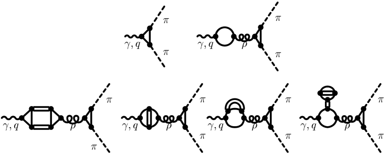
Figure 5: Contributions to the pion electromagnetic form factor. Note that the propagator denoted by the curly line corresponds to the $1/N_{c}$-corrected $rho$-meson, while the double lines indicate RPA pions and sigmas.

Evaluating the diagrams of Fig. 5 we obtain for the form factor

$$|F_{\pi}(q)|^{2}=\frac{1}{2}\,\Big{|}\,g_{\pi qq}^{(0)2}f(p,p^{\prime})\,\Big{(}1-{\tilde{\Pi}}_{\rho}(q){\tilde{D}}_{\rho}(q)\Big{)}\,\Big{|}^{2}~{},$$ (46)

where $p$ and $p^{\prime}$ are the four-momenta of the external pions and $f(p,p^{\prime})$ is a scalar function appearing in the $\pi\pi\rho$-vertex function (see App. C). For the form factor it has to be evaluated for on-shell pions, i.e. $p^{2}=p^{\prime 2}=m_{\pi}^{2}$ and $p\cdot p^{\prime}=q^{2}/2-m_{\pi}^{2}$. From its explicit form, which is given in App. C, one can show that $g_{\pi qq}^{(0)2}f(p,p^{\prime})=\sqrt{2}$ for $q^{2}=0$. Since the $\rho$-meson self energy ${\tilde{\Pi}}_{\rho}$ vanishes at this point, we find $F_{\pi}(0)=1$, as it should be.

Figure 6: The pion electromagnetic form factor (left panel) and the $\pi\pi$-phase shifts in the vector-isovector channel (right panel) for different meson cutoff parameters, $\Lambda_{M}=500$ MeV (dashed), $\Lambda_{M}=600$ MeV (solid) and $\Lambda_{M}=700$ MeV (dotted). The data points are taken from refs. [26] and [30], respectively.

The numerical results for $|F_{\pi}|^{2}$ as a function of the center-of-mass energy squared are displayed in the left panel of Fig. 6, together with the experimental data [26]. The various curves correspond to different values of the meson cutoff $\Lambda_{M}$. For the other parameters the values listed in Table 1 are taken. The vector coupling constant $g_{v}$ is chosen such that the maximum of the form factor is at the correct position. Roughly speaking this corresponds to fitting the mass of the (dressed) $\rho$-meson. We only show the results for $\Lambda_{M}\geq$ 500 MeV. For lower meson cutoffs the unphysical quark-antiquark decay threshold of the $\rho$-meson is below the maximum of the form factor and makes a comparison not very meaningful.

For $\Lambda_{M}$ = 500 MeV (dashed line) the quark-antiquark threshold is at $s$ = 0.63 GeV², causing a cusp in the form factor slightly above the maximum. Because of the sub-threshold attraction in the $\rho$-meson channel the form factor drops very steeply below the cusp, leading to a poor description of the data above the maximum. In addition, also at the rising edge of the peak, where threshold effects are less important, we see that the width of the form factor is underestimated by the calculation, i.e. $\Lambda_{M}$ is too small. On the other hand, a meson cutoff of 700 MeV (dotted line) is already too large. In particular, the height of the maximum is underestimated. With $\Lambda_{M}$ = 600 MeV (solid line) we obtain the best description of the data. Since we assumed exact isospin symmetry in our model we can, of course, not reproduce the detailed structure of the form factor around 0.61 GeV², which is due to $\rho$-$\omega$-mixing. The high-energy part above the peak is somewhat underestimated, mainly due to the $q\bar{q}$-threshold at $s$ = 0.80 GeV². Probably the fit can be somewhat improved if we take a slightly larger meson cutoff, but we are not interested in fine-tuning here. In addition, it is to be expected that the inclusion of $\rho$- and $a_{1}$ intermediate states will improve the high-energy behavior.

A closely related quantity is the charge radius of the pion, which is defined as

$$\langle{r_{\pi}^{2}}\rangle\;=\;6\,\frac{dF_{\pi}}{dq^{2}}\Big{|}_{q^{2}=0}\;.$$ (47)

Results for $\Lambda_{M}$ = 500, 600 and 700 MeV are listed in Table 1. All of them are close to the experimental value, $\langle{r_{\pi}^{2}}\rangle^{1/2}$ = (0.663 $\pm$ 0.006) fm [27]. For $\Lambda_{M}$ = 700 MeV we find perfect agreement. On the other hand, a simple pole ansatz for the form factor leads to $\langle{r_{\pi}^{2}}\rangle^{1/2}=\sqrt{6}/m_{\rho}$ = 0.63 fm [28], which is of the same quality as our results. Obviously, at $q^{2}$ = 0 we are not very sensitive to the details of the $\rho$-meson peak, while other effects which are not included in our model might start to play a role. Therefore the pion charge radius is certainly not very well suited for fixing our model parameters.

One can also look at the $\pi\pi$-phase shifts in the vector-isovector channel. We include the diagrams shown in Fig. 7, i.e. the s-channel $\rho$-meson exchange and the direct $\pi\pi$-scattering via a quark box diagram. The latter has to be projected onto spin and isospin 1, which is a standard procedure. (For example, the analogous projection onto spin and isospin 0 can be found in Refs. [22, 29].) Our results, together with the empirical data [30], are displayed in the right panel of Fig. 6. Since the main contribution comes from the s-channel $\rho$-meson exchange, they more or less confirm our findings for the form factor: below the $\rho$-meson peak the best fit of the data is obtained with $\Lambda_{M}$ = 600 MeV while, at higher energies, where $q\bar{q}$-threshold effects start to play a role, the data are better described with $\Lambda_{M}$ = 700 MeV.

Figure 7: Diagrams contributing to the $\pi\pi$-scattering amplitude: Quark box diagram (left) and s-channel $\rho$-meson exchange (right).

Finally, we wish to compare the results of the full $1/N_{c}$-corrected NJL model with the static limit, i.e. the approximation introduced in Sec. 4. As pointed out, this approximation corresponds to a purely hadronic description where all quark effects are suppressed. For instance, taking the static limit of the diagrams shown in Fig. 5, we exactly recover the diagrams which contribute to the pion electromagnetic form factor in the hadronic model of ref. [31]. On the other hand, we already estimated that quark effects should not be negligible, i.e. we expect the static limit not to be a good approximation to the exact NJL calculations. In fact, if we take the parameters of our best fit to the pion electromagnetic form factor ($\Lambda_{M}$ = 600 MeV) and insert the corresponding values for $m$ and $f_{\pi}^{(0)}$ (see Table 1) into Eq. (40) we find $g_{\rho\pi\pi}$ = 9.3, which is considerably larger than the value of $\sim 6$, typically needed in hadronic models to describe the data.

Figure 8: The imaginary part of the $1/N_{c}$-corrected $\rho$-meson propagator. The solid line represents the full calculation while the dashed line denotes the static limit.

Fig. 8 displays the imaginary part of the $\rho$-meson propagator for $\Lambda_{M}$ = 600 MeV. The solid line indicates the result of an exact treatment of our model. Since the parameters have been fitted to the pion electromagnetic form factor, the maximum is close to the empirical $\rho$-meson mass of 770 MeV. The cusp at $\sqrt{s}$ = 892 MeV is again a $q\bar{q}$-threshold effect. The corresponding result in the static limit is displayed by the dashed line. Of course there is no $q\bar{q}$-threshold in this approximation. Obviously the peak is much broader and shifted to higher energies.

For a better understanding of this behavior we also compare the real- and imaginary parts of the corresponding $\rho$-meson self-energies (Fig. 9). Obviously, the differences seen in Fig. 8 are mainly due to the real part which is much more attractive in the exact NJL calculation than in the static limit, while the imaginary parts are not very different up to $\sqrt{s}\sim$ 800 MeV. Note that, in this region, the imaginary part exclusively results from the $\rho\rightarrow\pi\pi$ process, i.e. quarks do not show up as unphysical decay channels. The differences to the static limit, both in the real- and in the imaginary part, come about by the fact, that the quarks cause a non-trivial momentum dependence of the intermediate meson propagators and of the effective meson-meson vertices. For instance, the quark triangles do not exactly behave as point-like three-meson vertices. This might be viewed as “physical quark effects” in contrast to the unphysical $q\bar{q}$-decays at higher energies. However, the momentum dependence of any quark loop below the $q\bar{q}$-threshold is related to the imaginary part above the threshold via dispersion relations. In that sense any difference to the static limit could be interpreted as an unphysical effect and one might ask whether “physical quark effects” exist at all. Of course, this fundamental question is far beyond the scope of our paper and can probably not be answered without understanding the mechanism of quark confinement itself. On the other hand, at sufficiently low energies ($\mathrel{\raise 1.29167pt\hbox{$<$\kern-7.5pt\lower 4.30554pt\hbox{$\sim$}}}$ 400 MeV) the exact self energy of the $\rho$ meson does indeed almost coincide with the static limit. Here one can nicely see, how a hadronic model, which incorporates chiral symmetry, emerges naturally from the underlying quark structure once the many-body theory is carried to a sufficient degree of sophistication.

Figure 9: The real part (left) and the imaginary part (right) of the $1/N_{c}$-corrected $\rho$-meson self-energy, multiplied by $-2g_{v}$. The solid line represents the full calculation, while the dashed line indicates the static limit.

6 Conclusions

We have investigated meson properties within the Nambu–Jona-Lasinio model, including meson-loop corrections, which are generated via a systematic $1/N_{c}$-expansion of the self energy in next-to-leading order. We have shown that such a scheme is consistent with chiral symmetry, leading to massless pions in the chiral limit. For non-vanishing current quark masses the pion mass is consistent with the Gell-Mann Oakes Renner relation if one carefully expands both sides of the relation up to next-to-leading order in $1/N_{c}$.

The relative importance of the $1/N_{c}$-corrections is controlled by a parameter $\Lambda_{M}$, which cuts off the three-momenta of the meson loops. One of the main goals of the present article was to determine the value of $\Lambda_{M}$, together with the other parameters of the model. To that end we have performed a fit of the quark condensate $\langle{\bar{\psi}\psi}\rangle$ and the pion decay constant $f_{\pi}$, together with the pion electromagnetic form factor $F_{\pi}$ in the time-like region. The latter more or less amounts to fitting the mass and the width of the $\rho$-meson. Here the meson loops are absolutely crucial in order to include the dominant $\rho\rightarrow\pi\pi$-decay channel, while the leading-order approximation contains only unphysical $q\bar{q}$-decay channels. Of course, a priori it was not clear to what extent these unphysical decay modes, which are an unavoidable consequence of the missing confinement mechanism in the NJL model, are still present in the region of the $\rho$-meson peak.

It turns out that a reasonable fit of the above observables can be achieved with $\Lambda_{M}$ = 600 MeV. For the constituent quark mass we find $m$ = 446 MeV. Hence the unphysical $q\bar{q}$-decay channel opens at 892 MeV, about 120 MeV above the maximum of the $\rho$-meson peak. Our result is also interesting in the context of Ref. [17] where we have reported on the existence of instabilities in the pion sector for very large values of $\Lambda_{M}$. However, with $\Lambda_{M}$ = 600 MeV, as determined by our parameter fit, we are far away from this region. In fact, we find only moderate changes in the pion and quark sector: $f_{\pi}$ and $\langle{\bar{\psi}\psi}\rangle$ are lowered by about 20% by the meson loop corrections, while the pion mass is increased by about 10%. This also indicates that our scheme converges rapidly and higher-order terms in the $1/N_{c}$-expansion are small.

We have discussed that a hadronic model can be derived from our model if one takes the so-called static limit. Basically, this corresponds to a low-momentum approximation to the quark loops. In this way one can study the importance of quark effects, which are present in the exact model because of lack of confinement, but absent in the static limit. At higher energies we find for the $\rho$-meson rather large differences between the exact propagator and the static limit, whereas at sufficiently low energies ($\mathrel{\raise 1.29167pt\hbox{$<$\kern-7.5pt\lower 4.30554pt\hbox{$\sim$}}}$ 400 MeV) the exact calculation and the static limit almost coincide. This implies that in the low-energy region the unphysical quark effects are suppressed and demonstrates that a hadronic model with realistic parameters indeed emerges from the underlying quark structure. It is likely that the quark threshold and hence the unphysical effects from continuum $\bar{q}q$ decay can be pushed to even higher energies once intermediate $\rho$-and $a_{1}$ meson states are included. Given the successful vacuum description of the $\rho$ meson, as presented in the present paper, it will be interesting to extend the calculation to finite temperature to asses medium modifications in the presence of a thermal heat bath. Because of spontaneous chiral symmetry breaking and its restoration at high temperature this implies a simultaneous treatment of the $a_{1}$ meson. Work in this direction is in progress.

Appendix A Definition of elementary integrals

It is possible to reduce the expressions for the quark loops to some elementary integrals [32], see App. B and C. In this section we give the definitions of these integrals.

$$I_{1}=\int\frac{d^{4}k}{(2\pi)^{4}}\frac{1}{k^{2}-m^{2}+i\varepsilon}~{},$$ (48)

$$I(p)=\int\frac{d^{4}k}{(2\pi)^{4}}\frac{1}{(k^{2}-m^{2}+i\varepsilon)((k+p)^{2}-m^{2}+i\varepsilon)}~{},$$ (49)

$$K(p)=\int\frac{d^{4}k}{(2\pi)^{4}}\frac{1}{(k^{2}-m^{2}+i\varepsilon)^{2}((k+p)^{2}-m^{2}+i\varepsilon)}~{},$$ (50)

$$M(p_{1},p_{2})=\int\frac{d^{4}k}{(2\pi)^{4}}\frac{1}{(k^{2}-m^{2}+i\varepsilon)(k_{1}^{2}-m^{2}+i\varepsilon)(k_{2}^{2}-m^{2}+i\varepsilon)}~{},$$ (51)

$$L(p_{1},p_{2},p_{3})=\int\frac{d^{4}k}{(2\pi)^{4}}\frac{1}{(k^{2}-m^{2}+i\varepsilon)(k_{1}^{2}-m^{2}+i\varepsilon)(k_{2}^{2}-m^{2}+i\varepsilon)(k_{3}^{2}-m^{2}+i\varepsilon)}~{},$$ (52)

$$p_{1}^{\mu}M_{1}(p_{1},p_{2})+p_{2}^{\mu}M_{1}(p_{2},p_{1})=\int\frac{d^{4}k}{(2\pi)^{4}}\frac{k^{\mu}}{(k^{2}-m^{2}+i\varepsilon)(k_{1}^{2}-m^{2}+i\varepsilon)(k_{2}^{2}-m^{2}+i\varepsilon)},$$ (53)

with $k_{i}=k+p_{i}$. The function $M_{1}(p_{1},p_{2})$ can be expressed in terms of the other integrals:

$$M_{1}(p_{1},p_{2})=\frac{p_{1}\!\cdot\!p_{2}\ I(p_{1})-p_{2}^{2}\ I(p_{2})+(p_{2}^{2}-p_{1}\!\cdot\!p_{2})\ I(p_{1}-p_{2})+p_{2}^{2}\ (p_{1}^{2}-p_{1}\!\cdot\!p_{2})\ M(p_{1},p_{2})}{2\;((p_{1}\!\cdot\!p_{2})^{2}\,-\,p_{1}^{2}\,p_{2}^{2})}~{},$$ (54)

All integrals in Eqs. (48) to (53), are understood to be regularized. In our model we use Pauli-Villars regularization with two regulators, i.e. we replace

$$\int\frac{d^{4}k}{(2\pi)^{4}}f(k;m)\;\longrightarrow\;\int\frac{d^{4}k}{(2\pi)^{4}}\sum_{j=0}^{2}c_{j}\,f(k;\mu_{j})~{},$$ (55)

with

$$\mu_{j}^{2}\;=\;m^{2}\;+\;j\,\Lambda_{q}^{2}~{};\qquad c_{0}=1,\quad c_{1}=-2,\quad c_{2}=1~{}.$$ (56)

One then gets the following relatively simple analytic expressions for the integrals $I_{1}$, $I(p)$ and $K(p)$:

$$I_{1}=\frac{-i}{16\pi^{2}}\sum_{j}c_{j}\,\mu_{j}^{2}\ln(\mu_{j}^{2})$$ (57)

$$I(p)=\frac{-i}{16\pi^{2}}\sum_{j}c_{j}\,\Big{(}x_{j1}\ln(x_{j1})+x_{j2}\ln(-x_{j2})+x_{j1}\ln(-p^{2}x_{j1})+x_{j2}\ln(p^{2}x_{j2})\Big{)}$$ (58)

$$I(p=0)=\frac{-i}{16\pi^{2}}\sum_{j}c_{j}\,\ln(\mu_{j}^{2})$$ (59)

$$K(p)=\frac{-i}{16\pi^{2}}\sum_{j}c_{j}\,\frac{1}{2p^{2}(x_{j1}-x_{j2})}\Big{(}-\ln(x_{j1})-\ln(-x_{j1})+\ln(x_{j2})+\ln(-x_{j2})\Big{)}~{},$$ (60)

with

$$x_{j1,2}={1\over 2}\pm{1\over 2}\sqrt{1-{4\mu_{j}^{2}\over p^{2}}}\;.$$ (61)

An analytic expression for the three-point function (Eq. 51) can be found in Refs. [33] and [34]. In certain kinematical regions the four-point function (eq. 52) is also known analytically [33, 34].

Appendix B RPA propagators

Using the definitions given in the previous section the gap equation (Eq. (2)) takes the form

$$m\;=\;m_{0}+2ig_{s}\ 4N_{c}N_{f}\ m\ I_{1}\;.$$ (62)

Similarly one can evaluate the quark-antiquark polarization diagrams (Eq. (3)) and calculate the RPA meson propagators. The results read:

$$D_{\sigma}(p) = \frac{-2g_{s}}{{m_{0}\over m}+2ig_{s}\ 2N_{c}N_{f}\ (p^{2}-4m^{2})\ I(p)}~{},$$ (63)

$$D_{\pi}(p) = \frac{-2g_{s}}{{m_{0}\over m}+2ig_{s}\ 2N_{c}N_{f}\ p^{2}\ I(p)}~{},$$ (64)

$$D_{\rho}(p) = \frac{-2g_{v}}{1+2ig_{v}\ {4\over 3}N_{c}N_{f}\ (-2m^{2}\ I(0)+(p^{2}+2m^{2})\ I(p))}~{},$$ (65)

$$D_{a_{1}}(p) = \frac{-2g_{v}}{1+2ig_{v}\ {4\over 3}N_{c}N_{f}\ (-2m^{2}\ I(0)+(p^{2}-4m^{2})\ I(p))}~{}.$$ (66)

We should comment on the $\rho$- and the $a_{1}$-propagator. A straight-forward evaluation of the vector polarization diagrams gives

$$\Pi_{\rho}(p)=-i{4\over 3}N_{c}N_{f}\ (-2I_{1}+(p^{2}+2m^{2})\ I(p))~{}.$$ (67)

Because of vector current conservation this function should vanish for $p^{2}$ = 0. This is only true if

$$m^{2}\,I(0)\;=\;I_{1}~{},$$ (68)

which is not the case if we regularize $I(p)$ and $I_{1}$ as described in App. A. This corresponds to the standard form of Pauli-Villars regularization in the NJL model [7]. Alternatively one could perform the replacement Eq. (55) for the entire polarization loop. In fact, this is more in the original sense of Pauli-Villars regularization [35]. Then the factor $m^{2}$ in Eq. (67) should be replaced by a factor $\mu_{j}^{2}$ inside the sum over regulators and one can easily show that Eq. (68) holds (see Eqs. (57) and (59)). However, this scheme would lead to even more severe problems: From the gap equation (Eq. 62) we conclude that $iI_{1}$ should be positive. On the other hand the pion decay constant in the chiral limit and in leading order in $1/N_{c}$ is given by [7]

$$f_{\pi}^{2(0)}\;=\;-2iN_{c}N_{f}\ m^{2}\ I(0)~{}.$$ (69)

which implies that $im^{2}I(0)$ should be negative. So irrespective of the regularization scheme Eq. (68) cannot be fulfilled if we want to get reasonable results for $m$ and $f_{\pi}^{(0)}$ at the same time. Therefore we choose the standard form of Pauli-Villars regularization in the NJL-model [7] and replace the term $I_{1}$ in Eq. (67) by hand by $m^{2}\ I(0)$. This leads to the $\rho$-meson propagator as given in Eq. (65). For consistency the $a_{1}$ has been treated in the analogous way.

Appendix C Explicit expressions for the meson-meson vertices

In this section we list the explicit formulae for the meson-meson vertices. We restrict ourselves to those combinations which are needed for the calculations presented in this article.

We begin with the three-meson vertices $\Gamma_{M_{1},M_{2},M_{3}}(q,p)$ (see Fig. 4):

$$-i\Gamma_{\sigma,\sigma,\sigma}(q,p) = i2mN\Big{(}I(p^{\prime})+I(q)+I(p)+(4m^{2}-\frac{1}{2}(p^{\prime 2}+p^{2}+q^{2}))M(p,-q)\Big{)}~{},$$

$$-i\Gamma^{ab}_{\pi,\pi,\sigma}(q,p) = i2mN\delta_{ab}\Big{(}I(p^{\prime})+p\!\cdot\!qM(p,-q)\Big{)}~{},$$

$$-i\Gamma^{\mu\lambda,ab}_{\rho,\rho,\sigma}(q,p) = \delta_{ab}h(q,p)\Big{(}g^{\mu\lambda}-\frac{p^{2}\,q^{\mu}q^{\lambda}\;+\;q^{2}\,p^{\mu}p^{\lambda}\;-\;p\!\cdot\!q\,(p^{\mu}q^{\lambda}+q^{\mu}p^{\lambda})}{p^{2}q^{2}\;-\;(p\!\cdot\!q)^{2}}\Big{)}~{},$$

$$h(q,p) = imN\Big{(}I(q)+I(p)-2I(p^{\prime})+(4m^{2}-2p\!\cdot\!q-p^{\prime 2})M(p,-q)\Big{)}~{},$$

$$-i\Gamma_{\pi,\pi,\rho}^{\mu,abc}(q,p) = \varepsilon_{abc}\Big{(}q^{\mu}f(q,p)-p^{\mu}f(p,q)\Big{)}~{},$$

$$f(q,p) = N\Big{(}-I(q)+p^{2}M(p,-q)+2p\!\cdot\!qM_{1}(q,-p)\Big{)}~{},$$ (70)

with $p^{\prime}=-p-q$ and $N=4N_{c}N_{f}$.

For the four-meson vertices we only need to consider the special cases needed for the diagrams (b) and (c) in Fig. 3:

$$-i\Gamma_{\sigma,\sigma,\sigma,\sigma}(q,p,-q) = -N\Big{\{}\frac{I(p-q)+I(p+q)}{2}+4m^{2}\ (M(p,q)+M(p,-q))$$

$$\hskip 28.45274pt+2\big{(}m^{2}\ (4m^{2}-p^{2}-q^{2})-\frac{p^{2}q^{2}}{4}\big{)}\ L(p,-q,p-q)\Big{\}}$$

$$-i\Gamma_{\sigma,\sigma,\sigma,\sigma}(q,p,-p) = -N\Big{\{}I(p+q)+I(0)+4m^{2}\big{(}K(p)+K(q)+2M(p,-q)\big{)}$$

$$\hskip 28.45274pt+2p\!\cdot\!qM(p,-q)-q^{2}K(q)-p^{2}K(p)$$

$$\hskip 28.45274pt+m^{2}\big{(}16m^{2}-4p^{2}-4q^{2}+\frac{p^{2}q^{2}}{m^{2}}\big{)}L(p,-q,0)\Big{\}}$$

$$-i\Gamma_{\sigma,\pi,\sigma,\pi}^{ab}(q,p,-q) = \delta_{ab}N\Big{\{}I(p+q)+I(p-q)+p^{2}(4m^{2}-q^{2})L(p,-q,p-q)\Big{\}}$$

$$-i\Gamma_{\sigma,\pi,\pi,\sigma}^{ab}(q,p,-p) = \delta_{ab}N\Big{\{}-I(p+q)-I(0)-(4m^{2}-q^{2})(K(q)-p^{2}L(p,-q,0))$$

$$\hskip 28.45274pt+p^{2}K(p)-2p\!\cdot\!q\ M(p,-q)\Big{\}}$$

$$-i\Gamma_{\pi,\pi,\pi,\pi}^{abcd}(q,p,-q) = -N\kappa_{abcd}\Big{\{}I(p+q)+I(p-q)-p^{2}q^{2}L(p,-q,p-q)\Big{\}}$$

$$-i\Gamma_{\pi,\pi,\pi,\pi}^{abcd}(q,p,-p) = -N\kappa_{abcd}\Big{\{}I(p+q)+I(0)-p^{2}K(p)$$

$$\hskip 48.36958pt-q^{2}K(q)+2p\!\cdot\!qM(p,-q)+p^{2}q^{2}L(p,-q,0)\Big{\}}$$

$$-i\Gamma_{\rho,\sigma,\rho,\sigma}^{ab}(q,p,-q) = -2\delta_{ab}N\Big{\{}I(p+q)+I(p-q)+2I(q)-p\!\cdot\!q(M(p,-q)-M(p,q))$$

$$\hskip 42.67912pt+(4m^{2}-2p^{2})(M(p,q)+M(p,-q))$$

$$\hskip 42.67912pt+m^{2}(8m^{2}-6p^{2}+4q^{2}+\frac{p^{4}-(p\!\cdot\!q)^{2}}{m^{2}})L(p,-q,p-q)\Big{\}}$$

$$-i\Gamma_{\rho,\sigma,\sigma,\rho}^{ab}(q,p,-q) = -2\delta_{ab}N\Big{\{}-I(p+q)-I(0)+(p^{2}-4m^{2})K(p)$$

$$\hskip 42.67912pt+(q^{2}+2m^{2})K(q)+(4m^{2}-2p\!\cdot\!q)M(p,-q)$$

$$\hskip 42.67912pt+m^{2}(8m^{2}-2p^{2}+4q^{2}-\frac{p^{2}q^{2}}{m^{2}})L(p,-q,0)\Big{\}}$$

$$-i\Gamma_{\rho,\pi,\rho,\pi}^{abcd}(q,p,-q) = 2N\kappa_{abcd}\Big{\{}-I(p+q)-I(p-q)-2I(q)$$

$$\hskip 42.67912pt+2p^{2}(M(p,q)+M(p,-q))+p\!\cdot\!q(M(p,-q)-M(p,q))$$

$$\hskip 42.67912pt+(2m^{2}p^{2}-p^{4}+(p\!\cdot\!q)^{2})L(p,-q,p-q)\Big{\}}$$

$$-i\Gamma_{\rho,\pi,\pi,\rho}^{abcd}(q,p,-q) = 2N\kappa_{abcd}\Big{\{}I(p+q)+I(0)-p^{2}K(p)-(q^{2}+2m^{2})K(q)$$ (71)

$$\hskip 42.67912pt+2p\!\cdot\!qM(p,-q)+p^{2}(2m^{2}+q^{2})L(p,-q,0)\Big{\}}~{},$$

with $\Gamma_{\rho,M,M,\rho}(q,p,-q)=g_{\mu\nu}\Gamma_{\rho,M,M,\rho}^{\mu\nu}(q,p,-q),\Gamma_{\rho,M,\rho,M}(q,p,-p)=g_{\mu\nu}\Gamma_{\rho,M,\rho,M}^{\mu\nu}(q,p,-p)$ and $\kappa_{abcd}=\delta_{ab}\delta_{cd}+\delta_{ad}\delta_{bc}-\delta_{ac}\delta_{bd}$.

References

-
[1]
G.E. Brown, Nucl. Phys. A 446 (1985) 12c;
G.E. Brown, M. Rho, W. Weise, Nucl. Phys. A 454 (1986) 669. - [2] M. Herrmann, B. Friman and W. Nörenberg, Nucl. Phys. A 560 (1993) 411.
- [3] R. Rapp and J. Wambach, preprint hep-ph/9909229, to be published in Adv. Nucl Phys..
- [4] T. Schäfer and E.V. Shuryak, Rev. Mod. Phys. 70 (1998) 323.
- [5] Y. Nambu and G. Jona-Lasinio, Phys. Rev. 122 (1961) 345; 124 (1961) 246.
- [6] U. Vogl and W. Weise, Progr. Part. and Nucl. Phys. 27 (1991) 195.
- [7] S.P. Klevansky, Rev. Mod. Phys. 64 (1992) 3.
- [8] T. Hatsuda and T. Kunihiro, Phys. Rep. 247 (1994) 221.
- [9] S. Krewald, K. Nakayama and J. Speth, Phys. Lett. B 272 (1991) 190.
- [10] E. Quack and S.P. Klevansky, Phys. Rev. C 49 (1994) 3283.
- [11] D. Blaschke, Yu.L. Kalinovsky, G. Röpke, S. Schmidt and M.K. Volkov, Phys. Rev. C 53 (1996) 2394.
- [12] V. Dmitrašinovic̀, H.-J. Schulze, R. Tegen and R.H. Lemmer, Ann. Phys. (NY) 238 (1995) 332.
- [13] E.N. Nikolov, W. Broniowski, C.V. Christov, G. Ripka and K. Goeke, Nucl. Phys. A 608 (1996) 411.
- [14] R.H. Lemmer and R. Tegen, Nucl. Phys. A 593 (1995) 315.
- [15] Y.B. He, J. Hüfner, S.P. Klevansky and P. Rehberg, Nucl. Phys. A 630 (1998) 719.
- [16] M. Huang, P. Zhuang and W. Chao, preprints hep-ph/9906468; hep-ph/9903304.
- [17] M. Oertel, M. Buballa and J. Wambach, preprint hep-ph/9908475.
- [18] H. Kleinert and B. Van den Bossche, preprints hep-ph/9907274; hep-ph/9908284.
- [19] S. Klimt, M. Lutz, U. Vogl and W. Weise, Nucl. Phys. A 516 (1990) 429.
- [20] G. Chanfray and P. Schuck, Nucl. Phys. A 555 (1993) 329.
- [21] N.M. Kroll, T.D. Lee and B. Zumino, Phys. Rev. 157 (1967) 1376.
- [22] D. Davesne, Y.J. Zhang and G. Chanfray, preprint nucl-th/9909032.
- [23] H.G. Dosch and S. Narison, Phys. Lett. B 417 (1998) 173.
- [24] L. Giusti, F. Rapuano, M. Talevi and A. Vladikas, Nucl. Phys. B 538 (1999) 249.
- [25] M. Lutz and W. Weise, Nucl. Phys. A 518 (1990) 156.
- [26] L.M. Barkov et al., Nucl. Phys. B 256 (1985) 365; S.R. Amendolia et al., Phys. Lett. B 138 (1984) 454.
- [27] S.R. Amendolia et al., Nucl. Phys. B 277 (1986) 168.
- [28] R.K. Bhaduri, Models of the Nucleon, Addison-Wesley, Redwood City, California 1988.
- [29] V. Bernard, U.-G. Meißner, A.H. Blin, B. Hiller, Phys. Lett. B 253 (1991) 443
- [30] C.D. Frogatt, J.L. Petersen, Nucl. Phys. B 129 (1977) 89
- [31] F. Klingl, N. Kaiser and W. Weise, Z. Phys. A 356 (1996) 193.
- [32] G. Passarino, M. Veltman, Nucl. Phys. B 160 (1979) 151.
- [33] G.J. van Oldenborgh, J.A.M. Vermaseren, Z. Phys. C 46 (1990) 425.
- [34] G. t’Hooft, M. Veltman, Nucl. Phys. B 153 (1979) 365.
- [35] C. Itzykson and J.-B. Zuber, Quantum Field Theory, McGraw-Hill, New York 1980.