Particle Interferometry from 40 MeV to 40 TeV

Abstract

Recent developments are summarized in the theory of Bose–Einstein and Fermi–Dirac correlations, with emphasis on the necessity of a simultaneous analysis of particle spectra and quantum statistical correlations for a detailed reconstruction of the space-time picture of particle emission. The reviewed topics are as follows: basics and formalism of quantum-statistical correlations, model-independent analysis of short-range correlations, Coulomb wave-function corrections and the core/halo picture for $n$-particle Bose–Einstein correlations, the graph rules to calculate these correlations even with partial coherence in the core; particle interferometry in e⁺e^- collisions including the Andersson–Hofmann model; the invariant Buda–Lund particle interferometry; the Buda–Lund, the Bertsch–Pratt and Yano–Koonin–Podgoretskii parameterizations, the Buda–Lund hydro model and its applications to ($\pi$/K) + p and Pb + Pb collisions at CERN SPS, and to low energy heavy ion collisions; the binary source formalism and the related oscillations in the two-particle Bose–Einstein and Fermi–Dirac correlation functions; the experimental signs of expanding rings of fire and shells of fire in particle and heavy ion physics and their similarity to planetary nebulae in stellar astronomy; the signal of partial restoration of the axial $U_{A}(1)$ symmetry restoration in the two-pion Bose–Einstein correlation function; the back-to-back correlations of bosons with in-medium mass modifications; and the analytic solution of the pion-laser model.

“Imagination is more important than knowledge.”

A. Einstein

1 Introduction

Although the concept of Bose–Einstein [1, 2] or intensity interferometry was discovered in particle and nuclear physics more than 30 years ago [3, 4], some basic questions in the field are still unanswered, namely, what the form of the Bose–Einstein correlation functions is, and what this form means. However, even if the ultimate understanding of the effect is still lacking, the level of sophistication in the theoretical descriptions and the level of sophistication in the experimental studies of Bose–Einstein correlations and particle interferometry has increased drastically, particularly in the field of heavy ion physics [5].

1.1 W-mass determination and particle interferometry

The study of Bose–Einstein correlations is interesting in its own right, but it should be noted that consequences may spill over into other fields of research, that are seemingly unrelated. Such is the topic of the W-mass determination at LEP2, a top priority research in high energy physics. It turned out that the non-perturbative Bose–Einstein correlations between the pions from decaying W⁺W^- pairs could be responsible for the presently largest systematic errors in W-mass determination at LEP2 [6, 7]. Hence, the theoretical understanding and the experimental control of Bose–Einstein correlations at LEP2 is essential to make a precision measurement of the W mass, which in turn may carry information via radiative corrections about the value of the Higgs mass or signals of new physics beyond the Standard Model.

1.2 Quark–gluon plasma and particle interferometry

Heavy ion physics is the physics of colliding atomic nuclei. At the presently largest energies, the aim of heavy ion physics is to study the sub-nuclear degrees of freedom by successfully creating and identifying the quark–gluon plasma (QGP). This presently only hypothetical phase of matter would consist of freely moving quarks and gluons, over a volume which is macroscopical relative to the characteristic 1 fm size of hadrons.

Theoretically proposed signals of the expected phase transition from hot hadronic matter to QGP were tested till now by fixed target experiments. At AGS, Brookhaven, collisions were made with nuclei as big as ¹⁹⁷Au accelerated to14.5 AGeV bombarding energy. At CERN SPS, collisions were made with 60 and 200 AGeV beams of ¹⁶O nuclei, 200 AGeV beams of ³²S nuclei, 40 and 158 AGeV beams of ²⁰⁸Pb nuclei [5]. The really heavy projectile runs were made relatively recently, the data are being published and the implications of the new measurements are explored theoretically, with claims of a possible QGP production at CERN SPS Pb + Pb reactions, however, without a clear-cut experimental proof of the identification of the new phase [5]. Both at CERN and at BNL, new collider experiments are planned and being constructed. The Relativistic Heavy Ion Collider (RHIC) at Brookhaven will collide $100+100$ AGeV ¹⁹⁷Au nuclei, which yields about 40 TeV total energy in the center of mass frame. RHIC started to deliver its first results in 2000. The construction stage of the RHIC accelerator rings was declared to be complete by the US Department of Energy on August 14, 1999, during a NATO Advanced Study Institute in Nijmegen, The Netherlands, where the material of this review paper has been presented. The forthcoming Large Hadron Collider (LHC) at CERN is scheduled to start in 2005. LHC will collide nuclei up to ²⁰⁸Pb with 2.76 + 2.76 ATeV bombarding energy, yielding a total energy of 1150 TeV in the center of mass frame. The status quo has been summarized recently in Refs [8, 9, 10, 11, 12, 13].

At such large bombarding energies, the sub-nuclear structure of matter is expected to determine the outcome of the experiments. However, the observed single particle spectra and two-particle correlations indicated rather simple dependences on the transverse mass of the produced particles [14, 15], that had a natural explanation in terms of hydrodynamical parameterizations. Although hydrodynamical type of models are also able to fit the final hadronic abundances, spectra and correlations, [9] these models are not able to describe the ignition part of the process, thus their predictions are dependent on the assumed initial state. The hydro models come in two classes: i) hydro parameterizations, that attempt to parameterize the flow, temperature and density distributions on or around the freeze-out hypersurface [16, 17, 18, 19, 20, 21, 22, 23, 24] by fitting the observed particle spectra and correlations, for example [19, 25, 28, 29, 30], but without solving the time-dependent (relativistic) hydrodynamical equations. The class ii) comes in the form of hydrodynamical solutions, that assume an equation of state and an initial condition, and follow the time evolution of the hydrodynamical system until a freeze-out hypersurface. These are better substantiated but more difficult to fit calculations, than class i) type of parameterizations. The exact hydro solutions are obtained either in analytical forms, [31, 32, 33, 34, 35, 36, 37, 38, 39, 40], or from numerical solutions, see for example Refs [41, 42, 43, 44]. An even more substantiated approach is hydrodynamical approach with continuous emission of particles, which takes into account the small sizes of heavy ion reactions as compared to the mean free path of the particles [45]. Such a continuous emission of hadrons during the time evolution of the hot and dense hadronic matter is supported by microscopic simulations [46].

In principle, the exact hydrodynamical solutions can be utilized in a time-reversed form: after fixing the parameters to describe the measured particle spectra and correlations at the time when the particles are produced, the hydro code can be followed backwards in time, and one may learn about the initial condition [47] in a given reaction: was it a QGP or a conventional hadron gas initial state?

1.3 Basics of quantum statistical correlations

Essentially, intensity correlations appear due to the Bose–Einstein or Fermi–Dirac symmetrization of the two-particle final states of identical bosons or fermions, in short, due to quantum statistics.

The simplest derivation is as follows: suppose that a particle pair is observed, one with momentum $k_{1}$ the other with momentum $k_{2}$. The amplitude has to be symmetrized over the unobservable variables, in particular over the points of emissions $x_{1}$ and $x_{2}$. If Coulomb, strong or other final-state interactions can be neglected, the amplitude of such a final state is proportional to

$$A_{12}\propto\frac{1}{\sqrt{2}}\,\,[\,{\rm e}^{ik_{1}x_{1}+ik_{2}x_{2}}\pm{\rm e}^{ik_{1}x_{2}+ik_{2}x_{1}}\,],$$ (1)

where $+$ sign stands for bosons, $-$ for fermions. If the particles are emitted in an incoherent manner, the observable two-particle spectrum is proportional to

$$N_{2}(k_{1},k_{2})\propto\int dx_{1}\rho(x_{1})\int dx_{2}\rho(x_{2})\,\,|A_{12}|^{2}$$ (2)

and the resulting two-particle intensity correlation function is

$$C_{2}(k_{1},k_{2})=\frac{N_{2}(k_{1},k_{2})}{N_{1}(k_{1})N_{2}(k_{2})}\,=1\pm|\tilde{\rho}(k_{1}-k_{2})|^{2}$$ (3)

that carries information about the Fourier-transformed space-time distribution of the particle emission

$$\tilde{\rho}(q)=\int dx\,\,{\rm e}^{iqx}\,\,\rho(x)$$ (4)

as a function of the relative momentum $q=k_{1}-k_{2}$.

As compared to the idealized case when quantum-statistical correlations are negligible (or neglected), Bose–Einstein or Fermi–Dirac correlations modify the momentum distribution of the hadron pairs in the final state by a weight factor $\langle 1\pm\rm\cos[(k_{1}-k_{2})\cdot(x_{1}-x_{2})]\rangle$.

1.4 Correlations between particle and heavy ion physics

In case of pions, that are produced abundantly in relativistic heavy ion experiments, Bose–Einstein symmetrization results in an enhancement of correlations of pion pairs with small relative momentum, and the correlation function carries information about the space-time distribution of pion production points. This in turn is expected to be sensitive to the formation of a transient quark–gluon plasma stage [48].

In particle physics, reshuffling or modification of the momentum of pions in the fully hadronic decays of the W⁺W^- pairs happens due to the Bose–Einstein symmetrization of the full final stage, that includes symmetrization of pions with similar momentum from different W-s. As a consequence of this quantum interference of pions, a systematic error as big as 100 MeV may be introduced to the W-mass determination from reconstruction of the invariant masses of $(\rm q\overline{\rm q})$ systems in 4-jet events [6, 7]. It is very difficult to handle the quantum interference of pions from the W⁺ and W^- jets with Monte-Carlo simulations, perturbative calculations and other conventional methods of high energy physics.

Unexpectedly, a number of recent experimental results arose suggesting that the Bose–Einstein correlations and the soft components of the single-particle spectra in high energy collisions of elementary particles show similar features to the same observables in high energy heavy ion physics [49, 50, 51, 52].

These striking similarities of multi-dimensional Bose–Einstein correlations and particle spectra in high energy particle and heavy ion physics have no fully explored dynamical explanation yet. This review intends to give a brief introduction to various sub-fields of particle interferometry, highlighting those phenomena that may have applications or analogies in various different type of reactions. The search for such analogies inspired a study of non-relativistic heavy ion reactions in the 30 – 80 AMeV energy domain and a search for new exact analytic solutions of fireball hydrodynamics, reviewed briefly for a comparison.

As some of the sections are mathematically more advanced, and other sections deal directly with data analysis, I attempted to formulate the various sections so that they be self-standing as much as possible, and be of interest for both the experimentally and the theoretically motivated readers.

2 Formalism

The basic properties of the Bose–Einstein $n$-particle correlation functions (BECF-s) can be summarized as follows, using only the generic aspects of their derivation.

The $n$-particle Bose–Einstein correlation function is defined as

$$C_{n}({\bf{k}}_{1},\cdots,{\bf{k}}_{n})={\displaystyle{\phantom{|}}N_{n}({\bf{k}}_{1},\cdots,{\bf{k}}_{n})\over\displaystyle{\phantom{|}}N_{1}({\bf{k}}_{1})\cdots N_{1}({\bf{k}}_{n})},$$ (5)

where $N_{n}({\bf{k}}_{1},\cdots,{\bf{k}}_{n})$ is the $n$-particle inclusive invariant momentum distribution, while

$$N_{n}({\bf{k}}_{1},\cdots,{\bf{k}}_{n})=\frac{1}{\sigma}E_{{\bf{k}}_{1}}\cdots E_{{\bf{k}}_{n}}\frac{d^{3n}\sigma}{d{{\bf{k}}}_{1}\cdots d{{\bf{k}}}_{n}}$$ (6)

is the invariant $n$-particle inclusive momentum distribution. It is quite remarkable that the complicated object of Eq. (5) carries quantum mechanical information on the phase-space distribution of particle production as well as on possible partial coherence of the source, can be expressed in a relatively simple, straight-forward manner both in the analytically solvable pion-laser model of Refs [53, 54, 55, 56] as well as in the generic boosted-current formalism of Gyulassy, Padula and collaborators [57, 58, 59] as

$$C_{n}({\bf{k}}_{1},\cdots,{\bf{k}}_{n})={\displaystyle{\phantom{|}}\sum_{\sigma^{(n)}}\prod_{i=1}^{n}G({\bf{k}}_{i},{\bf{k}}_{\sigma_{i}})\over\displaystyle{\phantom{|}}\prod_{i=1}^{n}G({\bf{k}}_{i},{\bf{k}}_{i})},$$ (7)

where $\sigma^{(n)}$ stands for the set of permutations of indices $(1,2,\cdots,n)$ and $\sigma_{i}$ denotes the element replacing element $i$ in a given permutation from the set of $\sigma^{(n)}$, and, regardless of the details of the two different derivations,

$$G({\bf{k}}_{i},{\bf{k}}_{j})=\sqrt{E_{{\bf{k}}_{i}}E_{{\bf{k}}_{j}}}\langle a^{\dagger}({\bf{k}}_{i})a({\bf{k}}_{j})\rangle$$ (8)

stands for the expectation value of $a^{\dagger}({\bf{k}}_{i})a({\bf{k}}_{j})$. The operator $a^{\dagger}({{\bf{k}}})$ creates while operator $a({{\bf{k}}})$ annihilates a boson with momentum ${{\bf{k}}}$. The quantity $G({\bf{k}}_{i},{\bf{k}}_{j})$ corresponds to the first order correlation function in the terminology of quantum optics. In the boosted-current formalism, the derivation of Eq. (7) is based on the assumptions that i) the bosons are emitted from a semi-classical source, where currents are strong enough so that the recoils due to radiation can be neglected, ii) the source corresponds to an incoherent random ensemble of such currents, as given in a boost-invariant formulation in Ref. [58], and iii) that the particles propagate as free plane waves after their production. Possible correlated production of pairs of particles is neglected here. Note also the recent clarification of the proper normalization of the two-particle Bose–Einstein correlations [60].

A formally similar result is obtained when particle production happens in a correlated manner, generalizing the results of Refs [54, 55, 56, 61, 62]. Namely, the $n$-particle exclusive invariant momentum distributions of the pion-laser model read as

$$N_{n}^{(n)}({\bf{k}}_{1},\cdots,{\bf{k}}_{n})=\sum_{\sigma^{(n)}}\prod_{i=1}^{n}G_{1}({\bf{k}}_{i},{\bf{k}}_{\sigma_{i}}),$$ (9)

with

$$G_{1}({\bf{k}}_{i}{\bf{k}}_{j})=\sqrt{E_{{\bf{k}}_{i}}E_{{\bf{k}}_{j}}}\mbox{Tr}\{\hat{\rho}_{1}a^{\dagger}({\bf{k}}_{i})a({\bf{k}}_{j})\},$$ (10)

where $\hat{\rho}_{1}$ is the single-particle density matrix in the limit when higher-order Bose–Einstein correlations are negligible. Q.H. Zhang has shown [62], that the $n$-particle inclusive spectrum has a similar structure:

$$N_{n}({\bf{k}}_{1},\cdots,{\bf{k}}_{n}) = \sum_{\sigma^{(n)}}\prod_{i=1}^{n}G({\bf{k}}_{i},{\bf{k}}_{\sigma_{i}})\,,$$ (11)

$$G({\bf{k}}_{i},{\bf{k}}_{j}) = \sum_{n=1}^{\infty}G_{n}({\bf{k}}_{i},{\bf{k}}_{j})\,.$$ (12)

This result, valid only if the density of pions is below a critical value [56], was obtained if the multiplicity distribution was assumed to be a Poissonian one in the rare gas limit. The formula of Eq. (12) has been generalized by Q.H. Zhang in Ref. [63] to the case when the multiplicity distribution in the rare gas limit is arbitrary.

The functions $G_{n}({\bf{k}}_{i},{\bf{k}}_{j})$ can be considered as representatives of order $n$ symmetrization effects in exclusive events where the multiplicity is fixed to $n$, see Refs [53, 54, 55, 56] for more detailed definitions. The function $G({\bf{k}}_{i},{\bf{k}}_{j})$ can be considered as the expectation value of $a^{\dagger}({\bf{k}}_{i})a({\bf{k}}_{j})$ in an inclusive sample of events, and this building block includes all the higher-order symmetrization effects. In the relativistic Wigner function formalism, in the plane wave approximation $G({\bf{k}}_{1},{\bf{k}}_{2})$ can be rewritten as

$$G({\bf{k}}_{1},{\bf{k}}_{2}) \equiv \tilde{S}(q_{12},K_{12})\,=\,\int d^{4}x\,S(x,K_{12})\,\exp(iq_{12}\cdot x)\,,$$ (13)

$$K_{12} = 0.5(k_{1}+k_{2})\,,$$ (14)

$$q_{12} = k_{1}-k_{2}\,,$$ (15)

where a four-vector notation is introduced, $k=(E_{{\bf{k}}},{\bf{k}})$, and the energy of quanta with mass $m$ is given by $E_{{\bf{k}}}=\sqrt{m^{2}+{\bf{k}}^{2}}$, the mass-shell constraint. Notation $a\cdot b$ stands for the inner product of four-vectors. In the following, the relative momentum four-vector shall be denoted also as $\Delta k=q=(q_{0},q_{x},q_{y},q_{z})=(q_{0},{{\bf{q}}})$, the invariant relative momentum is $Q=\sqrt{-q\cdot q}$.

The covariant Wigner transform of the source density matrix, $S(x,{{\bf{k}}})$ is a quantum-mechanical analogue of the classical probability that a boson is produced at a given $(x,k)$ point in the phase-space, where $x=(t,{{\bf{r}}})=(t,r_{x},r_{y},r_{z})$. The quantity $S(x,K_{12})$ corresponds to the off-shell extrapolation of $S(x,{{\bf{k}}})$, as $K_{12}^{0}\neq\sqrt{m^{2}+{\bf K}_{12}^{2}}$. Fortunately, Bose–Einstein correlations are non-vanishing at small values of the relative momentum $q$, where $K_{12}^{0}\simeq E_{{\bf K}_{12}}$. Due to the mass-shell constraints, $G$ depends only on 6 independent momentum components.

For the two-particle Bose–Einstein correlation function, Eqs (7,8,13) yield the following representation:

$$C_{2}({{\bf{k}}}_{1},{{\bf{k}}}_{2})=1+\frac{|\tilde{S}(q_{12},K_{12})|^{2}}{\tilde{S}(0,{{\bf{k}}}_{1})\,\tilde{S}(0,{{\bf{k}}}_{2})}.$$ (16)

Due to the unknown off-shell behavior of the Wigner functions, it is rather difficult to evaluate this quantity from first principles, in a general case.

When comparing model results to data, two kind of simplifying approximations are frequently made:

i) The on-shell approximation can be used for developing Bose–Einstein afterburners to Monte-Carlo event generators, where only the on-shell part of the phase-space is modeled. In this approximation, Eq. (16) is evaluated with the on-shell mean momentum, $\tilde{K}=(\sqrt{m^{2}+{\bf K}_{12}^{2}},{\bf K}_{12})$. This on-shell approximation was used e.g. in Ref. [64] to sample $S(x,\tilde{K})$ from the single-particle phase-space distribution given by Monte-Carlo event generators, and to calculate the corresponding Bose–Einstein correlation functions in a numerically efficient manner. The method yields a straightforward technique for the inclusion of Coulomb and strong final-state interactions as well, see e.g. Ref. [64].

ii) The smoothness approximation can be used when describing Bose–Einstein correlations from a theoretically parameterized model, e.g. from a hydrodynamical calculation. In this case, the analytic continuation of $S(x,{{\bf{k}}})$ to the off-shell values of $K$ is providing a value for the off-shell Wigner function $S(x,K_{12})$. However, in the normalization of Eq. (16), the product of two on-shell Wigner functions appear. In the smoothness approximation, one evaluates this product as a leading order Taylor series in $q$ of the exact expression $\tilde{S}(0,{\bf K}-{{\bf{q}}}/2)S(0,{\bf K}+{{\bf{q}}}/2)$. The resulting formula,

$$C_{2}({{\bf{k}}}_{1},{{\bf{k}}}_{2})=1+\frac{|\tilde{S}(q_{12},K_{12})|^{2}}{|\tilde{S}(0,K_{12})|^{2}},$$ (17)

relates the two-particle Bose–Einstein correlation function to the Fourier-transformed off-shell Wigner function $S(x,K)$. This provides an efficient analytic or numeric method to calculate the BECF from sources with known functional forms. The correction terms to the smoothness approximation of Eq. (17) are given in Ref. [23]. These corrections are generally on the 5% level for thermal like momentum distributions.

3 Model-Independent Analysis of Short-Range Correlations

Can one model-independently characterize the shape of two-particle correlation functions? Let us attempt to answer this question on the level of statistical analysis, without theoretical assumptions on the thermal or non-thermal nature of the particle emitting source. In this approach, the usual theoretical assumptions are not made, neither on the presence or the negligibility of Coulomb and other final-state interactions, nor on the presence or the negligibility of a coherent component in the source, nor on the presence or the negligibility of higher-order quantum statistical symmetrization effects, nor on the presence or the negligibility of dynamical effects (e.g. fractal structure of gluon-jets) on the short-range part of the correlation functions. The presentation follows the lines of Ref. [65]. The reviewed method is really model-independent, and it can be applied not only to Bose–Einstein correlation functions but to every experimentally determined function, which features the properties i) and ii) listed below.

The following experimental properties are assumed:

i) The measured function tends to a constant for large values of the relative momentum.

ii) The measured function has a non-trivial structure at a certain value of its argument.

The location of the non-trivial structure in the correlation function is assumed for simplicity to be close to $Q=0$.

The properties i) and ii) are well satisfied by e.g. the conventionally used two-particle Bose–Einstein correlation functions. For a critical review on the non-ideal features of short-range correlations, (e.g. non-Gaussian shapes in multi-dimensional Bose–Einstein correlation studies), we recommend Ref. [66].

The core/halo intercept parameter $\lambda_{*}$ is defined as the extrapolated value of the two-particle correlation function at $Q=0$, see Section 5 for greater details. It turns out that $\lambda_{*}$ is an important physical observable, related to the degree of partial restoration of $U_{A}(1)$ symmetry in hot and dense hadronic matter [67, 68], as reviewed in Section 15.

Various non-ideal effects due to detector resolution, binning, particle mis-identification, resonance decays, details of the Coulomb and strong final-state interactions etc. may influence this parameter of the fit. One should also mention, that if all of these difficulties are corrected for by the experiment, the extrapolated intercept parameter $\lambda_{*}$ for like-sign charged bosons is (usually) not larger, than unity as a consequence of quantum statistics for chaotic sources, even with a possible admixture of a coherent component. However, final-state interactions, fractal branching processes of gluon jets, or the appearance of one-mode or two-mode squeezed states [69, 70] in the particle emitting source might provide arbitrarily large values for the intercept parameter.

A really model-independent approach is to expand the measured correlation functions in an abstract Hilbert space of functions. It is reasonable to formulate such an expansion so that already the first term in the series be as close to the measured data points as possible. This can be achieved if one identifies [65, 71] the approximate shape (e.g. the approximate Gaussian or the exponential shape) of the correlation function with the abstract measure $\mu(t)dt$ in the abstract Hilbert-space ${\cal H}$. The orthonormality of the basis functions $\phi_{n}(t)$ in ${\cal H}$ can be utilized to guarantee the convergence of these kind of expansions, see Refs [65, 71] for greater details.

3.1 Laguerre expansion and exponential shapes

If in a zeroth order approximation the correlation function has an exponential shape, then it is an efficient method to apply the Laguerre expansion, as a special case of the general formulation of Refs [65, 71]:

$$C_{2}(Q)\! = \!{\cal N}\left\{1+\lambda_{L}\exp(-QR_{L})\left[1+c_{1}L_{1}(QR_{L})+\frac{c_{2}}{2!}L_{2}(QR_{L})+...\right]\right\}.$$

In this and the next subsection, $Q$ stands symbolically for any, experimentally chosen, one dimensional relative momentum variable. The fit parameters are the scale parameters ${\cal N}$, $\lambda_{L}$, $R_{L}$ and the expansion coefficients $c_{1}$, $c_{2}$, … . The $n$th order Laguerre polynomials are defined as

$$L_{n}(t) = \exp(t)\frac{d^{n}}{dt^{n}}t^{n}\exp(-t),$$ (19)

they form a complete orthogonal basis for an exponential measure as

$$\delta_{n,m} \propto \int_{0}^{\infty}dt\,\exp(-t)L_{n}(t)L_{m}(t).$$ (20)

The first few Laguerre polynomials are explicitly given as

$$L_{0}(t) = 1,$$ (21)

$$L_{1}(t) = t-1,$$ (22)

$$L_{2}(t) = t^{2}-4t+2,\,...\,.$$ (23)

As the Laguerre polynomials are non-vanishing at the origin, $C(Q=0)\neq 1+\lambda_{L}$. The physically significant core/halo intercept parameter $\lambda_{*}$ can be obtained from the parameter $\lambda_{L}$ of the Laguerre expansion as

$$\lambda_{*} = \lambda_{L}[1-c_{1}+c_{2}-...].$$ (24)

3.2 Edgeworth expansion and Gaussian shapes

If, in a zeroth-order approximation, the correlation function has a Gaussian shape, then the general form given in Ref. [72] takes the particular form of the Edgeworth expansion [71, 72, 73] as:

$$C(Q) = {\cal N}\left\{1+\lambda_{E}\exp(-Q^{2}R_{E}^{2})\right.\times$$ (25)

$$\left.\left[1+\frac{\kappa_{3}}{3!}H_{3}(\sqrt{2}QR_{E})+\frac{\kappa_{4}}{4!}H_{4}(\sqrt{2}QR_{E})+...\right]\right\}.$$

The fit parameters are the scale parameters ${\cal N}$, $\lambda_{E}$, $R_{E}$, and the expansion coefficients $\kappa_{3}$, $\kappa_{4}$, … that coincide with the cumulants of rank 3, 4, … of the correlation function. The Hermite polynomials are defined as

$$H_{n}(t) = \exp(t^{2}/2)\left(-\frac{d}{dt}\right)^{n}\exp(-t^{2}/2),$$ (26)

they form a complete orthogonal basis for a Gaussian measure as

$$\delta_{n,m} \propto \int_{-\infty}^{\infty}dt\,\exp(-t^{2}/2)H_{n}(t)H_{m}(t).$$ (27)

The first few Hermite polynomials are listed as

$$H_{1}(t) = t,$$ (28)

$$H_{2}(t) = t^{2}-1,$$ (29)

$$H_{3}(t) = t^{3}-3t,$$ (30)

$$H_{4}(t) = t^{4}-6t^{2}+3,\,...\,$$ (31)

The physically significant core/halo intercept parameter $\lambda_{*}$ can be obtained from the Edgeworth fit of Eq. (25) as

$$\lambda_{*} = \lambda_{E}\left[1+\frac{\kappa_{4}}{8}+...\right].$$ (32)

This expansion technique was applied in the conference contributions [71, 72] to the AFS minimum bias and 2-jet events to characterize successfully the deviation of data from a Gaussian shape. It was also successfully applied to characterize the non-Gaussian nature of the correlation function in two-dimensions in case of the preliminary E802 data in Ref. [71], and it was recently applied to characterize the non-Gaussian nature of the three-dimensional two-pion BECF in e${}^{+}+$ e^- reactions at LEP1 [52].

Figure 1 indicates the ability of the Laguerre expansions to characterize two well-known, non-Gaussian correlation functions [65]: the second-order short-range correlation function $D^{s}_{2}(Q)$ as determined by the UA1 and the NA22 experiments [74, 75]. The convergence criteria of the Laguerre and the Edgeworth expansions is given in Ref. [65].

Fig. 1.: Laguerre expansion of NA22 and UA1 short-range correlations $D_{2}^{s}$ is shown by the solid line. Dashed line stands for the best exponential fit, which clearly underestimates the strength of the measured points at low values of the squared invariant momentum difference $Q^{2}=-(k_{1}-k_{2})^{2}$. (Note the logarithmic horizontal and vertical scales.)

Table 1.: Laguerre fits to UA1 and NA22 two-particle correlations

	UA1	NA22
${\cal N}$	1.355 $\pm$ 0.003	0.95 $\pm$ 0.01
$\lambda_{L}$	1.23 $\pm$ 0.07	1.37 $\pm$ 0.10
$R_{L}$ [fm]	2.44 $\pm$ 0.12	1.35 $\pm$ 0.14
$c_{1}$	0.52 $\pm$ 0.03	0.63 $\pm$ 0.06
$c_{2}$	0.45 $\pm$ 0.04	0.44 $\pm$ 0.06
$\chi^{2}/NDF$	41.2/41 = 1.01	20.0/34 = 0.59

From Table 1 the core/halo model intercept parameter is obtained as $\lambda_{*}=1.14\pm 0.10$ (UA1) and $\lambda_{*}=1.11\pm 0.17$ (NA22). As both of these values are within errors equal to unity, the maximum of the possible value of the intercept parameter $\lambda_{*}$ in a fully chaotic source, we conclude that either there are other than Bose–Einstein short-range correlations observed by both collaborations, or the full halo of long lived resonances is resolved in case of this measurement [76, 77, 78, 79].

If the two-particle BECF can be factorized as a product of (two or more) functions of one variable each, then the Laguerre and the Edgeworth expansions can be applied to the multiplicative factors — functions of one variable, each. This method was applied recently to study the non-Gaussian features of multi-dimensional Bose–Einstein correlation functions e.g. in Refs [52, 72]. The full, non-factorized form of two-dimensional Edgeworth expansion and the interpretation of its parameters is described in the handbook on mathematical statistics by Kendall and Stuart [80].

4 Coulomb Wave Corrections for Higher-Order Correlations

The short-range part of the two- and multi-particle correlation function of charged particles is strongly effected by Coulomb interactions. Even in the non-relativistic case, the $n$-body Coulomb scattering problem is solvable exactly only for the $n=2$ case, the full 3-body Coulomb wave-function is unknown. However, when studying higher-order Bose–Einstein correlations and e.g. searching for the onset of (partial) coherence in the source, it is desired that the Coulomb-induced correlations be removed from the data.

Fig. 2.: Coulomb wave-function correction factor and generalized Gamow correction factor for 5-particle correlation functions, for a Gaussian source with $R_{G}=5$ fm

In any given frame, the boost-invariant decomposition of Eq. (13) can be rewritten into the following, seemingly not invariant form:

$$G({\bf{k}}_{1},{\bf{k}}_{2}) = \int d^{3}{\bf x}\,\,S_{{\bf K}_{12}}({\bf x})\,\,\exp(i{\bf q}_{12}{\bf x}),$$ (33)

$$S_{{\bf K}_{12}}({\bf x}) = \int dt\,\exp(-i{\mbox{\boldmath$\beta$}}_{K_{12}}{\bf q}_{12}t)\,\,S({\bf x},t,K_{12}),$$ (34)

$${\mbox{\boldmath$\beta$}}_{K_{12}} = ({\bf k}_{1}+{\bf{k}}_{2})/(E_{1}+E_{2}).$$ (35)

Note that the relative source function $S_{{\bf K}_{12}}({\bf x})$ reduces to a simple time integral over the source function $S(x,K)$ in the frame where the mean momentum of the pair (hence the pair velocity ${\mbox{\boldmath$\beta$}}_{K_{12}}$) vanishes.

Based on a Poisson cluster picture, the effect of multi-particle Coulomb final-state interactions on higher-order intensity correlations is determined in general in Ref. [81], with the help of a scattering wave function which is a solution of the $n$-body Coulomb Schrödinger equation in (a large part of) the asymptotic region of the $n$-body configuration space.

If $n$ particles are emitted with similar momenta, so that their $n$-particle Bose–Einstein correlation functions may be non-trivial, Eqs (33–35) form the basis for evaluation of the Coulomb and strong final-state interaction effects on the observables for any given cluster of particles, assuming that the relative motion of the particles is non-relativistic within the cluster, see Ref. [81]. The Coulomb correction factor $K^{-1}$ can be integrated for arbitrary large number of particles and for any kind of model source, by replacing the plane wave approximation with the approximate $n$-body Coulomb wave-function. In the limit of vanishing source sizes, the generalization of the Gamow penetration factor was obtained to the correlation function of arbitrary large number of particles [81]. In particular, Coulomb effects on the $n$-particle Bose–Einstein correlation functions of similarly charged particles were studied for Gaussian effective sources, for $n=3$ in Ref. [82] and for $n=4$ and 5 in Ref. [81]. For the typical $R=1$ fm effective source sizes of the elementary particle reactions, the generalized $n$-body Gamow penetration factor gave rather precise estimates of the Coulomb correction (within 5% from the Coulomb-wave correction). In contrast, for typical effective source sizes observed in high energy heavy ion reactions, Fig. 2 indicates that the new Coulomb wave-function integration method allows for a removal of a systematic error as big as 100% from higher-order multi-particle Bose–Einstein correlation functions. See Ref. [81] for greater details.

5 Core/Halo Picture of Bose–Einstein Correlations

The core/halo model [76, 83, 84, 85, 86] deals with the consequences of a phenomenological situation, when the boson source can be considered to be a superposition of a central core surrounded by an extended halo. In the forthcoming sections, final-state interactions are neglected, we assume that the data are corrected for final-state Coulomb (and possibly strong) interactions.

Bose–Einstein correlations are measured at small relative momenta of particle pairs. In order to reliably separate the near-by tracks of particle pairs in the region of the Bose enhancement, each experiment imposes a cut-off $Q_{\rm min}$, the minimum value of the resolvable relative momentum. The value of this cut-off may vary slightly from experiment to experiment, but such a cut-off exists in each measurement.

In the core/halo model, the following assumptions are made:

Assumption 0: The emission function does not have a no-scale, power-law-like structure. This possibility was discussed and related to intermittency and effective power-law shapes of the two-particle Bose–Einstein correlation functions in Ref. [79].

Assumption 1: The bosons are emitted either from a central part or from the surrounding halo. Their emission functions are indicated by $S_{c}(x,{\bf k})$ and $S_{h}(x,{\bf k})$, respectively. According to this assumption, the complete emission function can be written as

$$S(x,{\bf k})=S_{c}(x,{\bf k})+S_{h}(x,{\bf k}),$$ (36)

and $S(x,{\bf k})$ is normalized to the mean multiplicity, $\int d^{4}x{\displaystyle\phantom{|}(d{\bf k}/E)}S(x,{\bf k})\,=\,\langle n\rangle$.

Assumption 2: The emission function that characterizes the halo is assumed to change on a scale $R_{h}$ that is larger than $R_{\rm max}\approx\hbar/Q_{\rm min}$, the maximum length-scale resolvable [76] by the intensity interferometry microscope. The smaller central core of size $R_{c}$ is assumed to be resolvable,

$$R_{h}>R_{\rm max}>R_{c}\,.$$ (37)

This inequality is assumed to be satisfied by all characteristic scales in the halo and in the central part, e.g. in case the side, out or longitudinal components [48, 87] of the correlation function are not identical.

Assumption 3: The core fraction $f_{c}({\bf k})=N_{c}({\bf k})/N_{1}({\bf k})$ varies slowly on the relative momentum scale given by the correlator of the core [85].

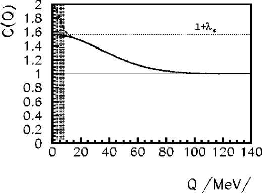
Fig. 3.: The shape of the BECF is illustrated for a source containing a core and a large halo. The contribution from the halo is restricted to the shaded area, while the shape of the BECF outside this interval is determined completely by the contribution of the core. If the resolution for a given experiment is restricted to $Q>10$ MeV, then an effective and momentum dependent intercept parameter, $\lambda_{*}(y,m_{t})$ will be measured, which can be combined with the measured momentum distribution to determine the the momentum distribution of the particles emitted directly from the core.

The emission function of the core and the halo are normalized as

$$\int d^{4}x{\displaystyle\phantom{|}d{\bf k}\over\displaystyle E}S_{c}(x,{\bf k})\,=\,\langle n\rangle_{c} \int d^{4}x{\displaystyle\phantom{|}d{\bf k}\over\displaystyle E}S_{h}(x,{\bf k})\,=\,\langle n\rangle_{h}.$$ and (38)

One finds [76, 85] that

$$N_{1}({\bf k})\,=\,N_{c}({\bf k})+N_{h}({\bf k}) \langle n\rangle\,=\,\langle n\rangle_{c}+\langle n\rangle_{h}.$$ and (39)

Note that in principle the core as well as the halo part of the emission function could be decomposed into more detailed contributions, e.g.

$$\vspace*{-6pt}S_{h}(x,{\bf k}) = \sum_{r=\omega,\eta,\eta^{\prime},K^{0}_{S}}S^{(r)}_{\rm halo}(x,{\bf k}).\vspace*{-6pt}$$ (40)

In case of pions and NA44 acceptance, the $\omega$ mesons were shown to contribute to the halo, Ref. [78]. For the present considerations, this separation is indifferent, as the halo is defined with respect to $Q_{\rm min}$, the experimental two-track resolution. For example, if $Q_{\rm min}=10-15$ MeV, the decay products of the $\omega$ resonances can be taken as parts of the halo [78]. If future experimental resolution decreases below $5$ MeV and the error bars on the measurable part of the correlation function decrease significantly in the $Q<\hbar/\Gamma_{\omega}=8$ MeV region, the decay products of the $\omega$ resonances will contribute to the resolvable core, see Refs [76, 78] for greater details.

If Assumption 3 is also satisfied by some experimental data set, then Eq. (16) yields a particularly simple form of the two-particle Bose–Einstein correlation function:

$$C_{2}({\bf k}_{1},{\bf k}_{2}) = 1+\lambda_{*}({\bf K}){\displaystyle\phantom{|}\mid\tilde{S}_{c}({\Delta k},{\bf K})\mid^{2}\over\displaystyle\tilde{S}_{c}(0,{\bf k}_{1})\tilde{S}_{c}(0,{\bf k}_{2})},$$ (41)

$$\simeq \,1+\lambda_{*}({\bf K}){\displaystyle\phantom{|}\mid\tilde{S}_{c}({\Delta k},{K})\mid^{2}\over\displaystyle|\tilde{S}_{c}(0,{K})|^{2}},$$ (42)

where mean and the relative momentum four-vectors are defined as

$$K=0.5(k_{1}+k_{2}),\qquad\Delta k=k_{1}-k_{2},$$ (43)

with $K=(K^{0},{\bf K})$ and $\Delta k=(\Delta k^{0},{\bf\Delta k})$, and the effective intercept parameter $\lambda_{*}({\bf K})$ is given as

$$\lambda_{*}({\bf K})=\left[N_{c}({\bf K})/N_{1}({\bf K})\right]^{2}.$$ (44)

As emphasized in Ref. [76], this effective intercept parameter $\lambda_{*}$ shall in general depend on the mean momentum of the observed boson pair, which within the errors of $Q_{\rm min}$ coincides with any of the on-shell four-momentum $k_{1}$ or $k_{2}$. Note that $\lambda_{*}\neq\lambda_{xct}=1$, the latter being the exact intercept parameter at $Q=0$ MeV. The core/halo model is summarized in Fig. 3, see Ref. [76] for further details. The core/halo model correlation function is compared to the so-called “model-independent”, Gaussian approximation of Refs [22, 23, 13] and to the full correlation function in Fig. 4, see appendix of Ref. [18] and that of Ref. [77] for further details.

The measured two-particle BECF is determined for $\mid{\bf\Delta k}\mid>Q_{\rm min}\approx 10$ MeV/c, and any structure within the $\mid{\bf\Delta k}\mid<Q_{\rm min}$ region is not resolved. However, the $(c,h)$ and $(h,h)$ type boson pairs create a narrow peak in the BECF exactly in this $\Delta k$ region according to Eq. (36), which cannot be resolved according to Assumption 2.

The general form of the BECF of systems with large halo, Eq. (42), coincides with the most frequently applied phenomenological parameterizations of the BECF in high energy heavy ion as well as in high energy particle reactions [89]. Previously, this form has received a lot of criticism from the theoretical side, claiming that it is in disagreement with quantum statistics [90] or that the $\lambda$ parameter is just a kind of fudge parameter, “a measure of our ignorance”. In the core/halo picture, Eq. (42) is derived with a standard inclusion of quantum statistical effects. Reactions including e${}^{+}+$ e^- annihilations, lepton–hadron and hadron–hadron reactions, nucleon–nucleus and nucleus–nucleus collisions are phenomenologically well described [89] by a core/halo picture.

Fig. 4.: Comparison of the full correlation function (full line) to the core/halo model approximation (dashed line) and to the “model-independent” Gaussian approximation (dotted line)

5.1 Partial coherence and higher-order correlations

In earlier studies of the core/halo model [76, 85] it was assumed that $S_{c}(x,p)$ describes a fully incoherent (thermal) source. In Ref. [86] an additional assumption was also made:

Assumption 4: A part of the core may emit bosons in a coherent manner:

$$S_{c}(x,{\bf{k}})=S_{c}^{p}(x,{\bf{k}})+S_{c}^{i}(x,{\bf{k}}),$$ (45)

where upper index $p$ stands for coherent component (which leads to partial coherence), upper index $i$ stands for incoherent component of the source.

The invariant spectrum is given by

$$N({\bf{k}})=\int d^{4}xS(x,{\bf{k}})=N_{c}({\bf{k}})+N_{h}({\bf{k}})$$ (46)

and the core contribution is a sum:

$$N_{c}({\bf{k}})=\int d^{4}xS_{c}(x,{\bf{k}})=N_{c}^{p}({\bf{k}})+N_{c}^{i}({\bf{k}}).$$ (47)

One can introduce the momentum dependent core fractions $f_{c}({\bf{k}})$ and partially coherent fractions $p({\bf{k}})$ as

$$f_{c}({\bf{k}}) = N_{c}({\bf{k}})/N({\bf{k}}),$$ (48)

$$p_{c}({\bf{k}}) = N_{c}^{p}({\bf{k}})/N_{c}({\bf{k}}).$$ (49)

Hence the halo and the incoherent fractions $f_{h},p_{i}$ are

$$f_{h}({\bf{k}}) = N_{h}({\bf{k}})/N({\bf{k}})=1-f_{c}({\bf{k}}),$$ (50)

$$f_{i}({\bf{k}}) = N_{c}^{i}({\bf{k}})/N_{c}({\bf{k}})=1-p_{c}({\bf{k}}).$$ (51)

5.2 Strength of the $n$-particle correlations

We denote the $n$-particle correlation function of Eq. (5) as

$$C_{n}(1,2,...,n) = C_{n}({\bf{k}}_{1},{\bf{k}}_{2},...,{\bf{k}}_{n})\,=\,\frac{N_{n}(1,2,...,n)}{N_{1}(1)N_{1}(2)...N_{1}(n)},$$ (52)

where a symbolic notation for ${\bf{k}}_{i}$ is introduced, only the index of ${\bf{k}}$ is written out in the argument. In the forthcoming, we shall apply this notation consistently for the arguments of various functions of the momenta, i.e. $f({\bf{k}}_{i},{\bf{k}}_{j},...,{\bf{k}}_{m})$ is symbolically denoted by $f(i,j,...,m)$.

The strength of the $n$-particle correlation function (extrapolated from a finite resolution measurement to zero relative momentum for each pair) is denoted by $C_{n}(0)$, given [86] by the following simple formula,

$$C_{n}(0)=1+\sum_{j=2}^{n}{\left({}^{\displaystyle\phantom{|}n}_{\displaystyle\phantom{|}j}\right)}\alpha_{j}f_{c}^{j}\left[(1-p_{c})^{j}+jp_{c}(1-p_{c})^{j-1}\right].$$ (53)

Here, $\alpha_{j}$ indicates the number of permutations, that completely mix exactly $j$ non-identical elements. There are $\left({}^{n}_{j}\right)$ different ways to choose $j$ different elements from among $n$ different elements. Since all the $n!$ permutations can be written as a sum over the fully mixing permutations, the counting rule yields a recurrence relation for $\alpha_{j}$, Refs [85, 86]:

$$\alpha_{n} = n!-\sum_{j=0}^{n-1}{\left({}^{\displaystyle\phantom{|}n}_{\displaystyle\phantom{|}j}\right)}\alpha_{j},$$ (54)

$$\alpha_{0} = 1.$$ (55)

The first few values of $\alpha_{j}$ are given as

$$\alpha_{1}=0,\quad\alpha_{2}=1,\quad\alpha_{3}=2,\quad\alpha_{4}=9,\quad\alpha_{5}=44,\quad\alpha_{6}=265,$$ (56)

the first few intercept parameters, $\lambda_{*,n}=C_{n}(0)-1$, are given as

$$\lambda_{*,2} = f_{c}^{2}[(1-p_{c})^{2}+2p_{c}(1-p_{c})],$$ (57)

$$\lambda_{*,3} = 3f_{c}^{2}[(1-p_{c})^{2}+2p_{c}(1-p_{c})]$$ (58)

$$\qquad+2f_{c}^{3}[(1-p_{c})^{3}+3p_{c}(1-p_{c})^{2}],$$

$$\lambda_{*,4} = 6f_{c}^{2}[(1-p_{c})^{2}+2p_{c}(1-p_{c})]$$ (59)

$$\qquad+8f_{c}^{3}[(1-p_{c})^{3}+3p_{c}(1-p_{c})^{2}]$$

$$\qquad+9f_{c}^{4}[(1-p_{c})^{4}+4p_{c}(1-p_{c})^{3}],$$

$$\lambda_{*,5} = 10f_{c}^{2}[(1-p_{c})^{2}+2p_{c}(1-p_{c})]$$ (60)

$$\qquad+20f_{c}^{3}[(1-p_{c})^{3}+3p_{c}(1-p_{c})^{2}]$$

$$\qquad+45f_{c}^{4}[(1-p_{c})^{4}+4p_{c}(1-p_{c})^{3}]$$

$$\qquad+44f_{c}^{5}[(1-p_{c})^{5}+5p_{c}(1-p_{c})^{4}].$$

In general, terms proportional to $f_{c}^{j}$ in the incoherent case shall pick up an additional factor $[(1-p_{c})^{j}+jp_{c}(1-p_{c})^{j-1}]$ in case the core has a coherent component [85, 86]. This extra factor means that either all $j$ particles must come from the incoherent part of the core, or one of them must come from the coherent, the remaining $j-1$ particles from the incoherent part. If two or more particles come from the coherent component of the core, the contribution to intensity correlations vanishes as the intensity correlator for two coherent particles is zero [88].

If the coherent component is present, one can introduce the normalized incoherent and partially coherent core fractions as

$$\tilde{s}_{c}^{i}(j,k) = {\tilde{S}^{i}_{c}(j,k)\over\tilde{S}^{i}_{c}(j,j)},$$ (61)

$$\tilde{s}_{c}^{p}(j,k) = {\tilde{S}^{p}_{c}(j,k)\over\tilde{S}^{p}_{c}(j,j)}.$$ (62)

In the partially coherent core/halo picture, one obtains the following closed form for the order $n$ Bose–Einstein correlation functions [86]:

$$C_{n}(1,...,n)\! = \!1+\sum_{j=2}^{n}\sum_{m_{1}...m_{j}=1}^{\hbox{}\,\,\,n\,\,\,_{\prime}}\sum_{\rho^{(j)}}\left\{\prod_{k=1}^{j}f_{c}(m_{k})[1-p_{c}(m_{k})]\,\,\tilde{s}^{i}_{c}(m_{k},m_{\rho_{k}})\right.$$ (63)

$$\hbox{}\left.+\sum_{l=1}^{j}f_{c}(m_{l})p_{c}(m_{l})\,\,\tilde{s}^{p}_{c}(m_{l},m_{\rho_{l}})\!\prod_{k=1,k\neq l}^{j}\!\!f_{c}(m_{k})[1-p_{c}(m_{k})]\,\tilde{s}^{i}_{c}(m_{k},m_{\rho_{k}})\right\}.$$

Here, $\rho^{(j)}$ stands for the set of permutations that completely mix exactly $j$ elements, $\rho_{i}$ stands for the permuted value of index $i$ in one of these permutations. By definition, $\rho_{i}\neq i$ for all $i=1,2,...,j$. The notation $\Sigma^{\prime}$ indicates summation for different values of indexes, $m_{i}\neq m_{l}$ for all $i,l$ pairs. The expression Eq. (63) contains two (momentum dependent) phases in the Fourier-transformed, normalized source distributions: one denoted by $\phi^{i}({\bf{k}}_{m},{\bf{k}}_{n})$ in the Fourier-transformed normalized incoherent core emission function, $\tilde{s}_{c}^{i}({\bf{k}}_{m},{\bf{k}}_{n})$ and another independent phase denoted by $\phi^{c}({\bf{k}}_{m},{\bf{k}}_{n})$ is present in the the Fourier-transformed normalized coherent core emission function, $\tilde{s}_{c}^{p}({\bf{k}}_{m},{\bf{k}}_{n})$. One can write

$$\tilde{s}_{c}^{i}({\bf{k}}_{m},{\bf{k}}_{n}) = |\tilde{s}_{c}^{i}({\bf{k}}_{m},{\bf{k}}_{n})|\exp[i\phi^{i}({\bf{k}}_{m},{\bf{k}}_{n})],$$ (64)

$$\tilde{s}_{c}^{p}({\bf{k}}_{m},{\bf{k}}_{n}) = |\tilde{s}_{c}^{p}({\bf{k}}_{m},{\bf{k}}_{n})|\exp[i\phi^{p}({\bf{k}}_{m},{\bf{k}}_{n})].$$ (65)

The shape of both the coherent and the incoherent components is arbitrary, but corresponds to the space-time distribution of particle production. If the variances of the core are finite, the emission functions can be parameterized by Gaussians, for the sake of simplicity [78]. If the core distributions have power-law-like tails, like in case of the Lorentzian distribution [18], then the Fourier-transformed emission functions correspond to exponentials or to power-law structures. For completeness, we list these possibilities below:

$$|\tilde{s}_{c}^{i}({\bf{k}}_{m},{\bf{k}}_{n})|^{2} = \exp(-R_{i}^{2}Q_{mn}^{2})\qquad\!\mbox{\rm or}$$ (66)

$$|\tilde{s}_{c}^{i}({\bf{k}}_{m},{\bf{k}}_{n})|^{2} = \exp(-R_{i}Q_{mn})\qquad\mbox{\rm or}$$ (67)

$$|\tilde{s}_{c}^{i}({\bf{k}}_{m},{\bf{k}}_{n})|^{2} = a_{i}(R_{i}Q_{mn})^{b_{i}}\qquad\ \ \mbox{\rm etc ... , }$$ (68)

$$|\tilde{s}_{c}^{p}({\bf{k}}_{m},{\bf{k}}_{n})|^{2} = \exp(-R_{p}^{2}Q_{ij}^{2})\qquad\ \ \!\mbox{\rm or}$$ (69)

$$|\tilde{s}_{c}^{p}({\bf{k}}_{m},{\bf{k}}_{n})|^{2} = \exp(-R_{p}Q_{mn})\qquad\mbox{\rm or}$$ (70)

$$|\tilde{s}_{c}^{p}({\bf{k}}_{m},{\bf{k}}_{n})|^{2} = a_{p}(R_{p}Q_{mn})^{b_{p}}\qquad\ \ \!\mbox{\rm etc ... }.$$ (71)

In the above equations, subscripts $i$ and $p$ index the parameters belonging to the incoherent or to the partially coherent components of the core, and $Q_{mn}$ stands for certain experimentally defined relative momentum component determined from ${\bf{k}}_{m}$ and ${\bf{k}}_{n}$.

A straightforward counting yields that in the limiting case when all momenta are equal, the simple formula of Eq. (53) follows from the shape of the $n$-particle Bose–Einstein correlation functions of Eq. (63), as $\tilde{s}^{i}_{c}(i,i)=\tilde{s}^{p}_{c}(i,i)=1$.

5.3 Graph rules

Graph rules were derived for the evaluation of the $n$-particle correlation function $C_{n}({\bf{k}}_{1},...,{\bf{k}}_{n})$ in Ref. [86]. Graphs contributing to the $n$ = 2 and 3 case are shown in Fig. 5, the case of $n=4$ is shown in Fig. 6.

Fig. 5.: Graphs determining the second and the third order correlation function for partially coherent core/halo sources

Circles can be either open or full. Each circle carries one label (e.g. $j$) standing for a particle with momentum ${\bf{k}}_{j}$. Full circles represent the incoherent core component by a factor $f_{c}(j)[1-p_{c}(j)]$, whereas open circles correspond to the coherent component of the core, a factor of $f_{c}(j)p_{c}(j)$.

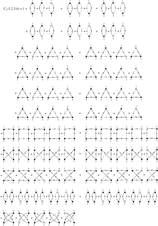
Fig. 6.: Graphs determining the fourth order correlation function for partially coherent core/halo sources

For the $n$-particle correlation function, all possible $j$-tuples of particles have to be found. Such $j$-tuples can be chosen in ${\left({}^{n}_{j}\right)}$ different manner. In a $j$-tuple, either each circle is filled, or the circle with index $k$ is open and the other $j-1$ circle is filled, which gives $j+1$ different possibilities. All the permutations that fully mix either $j=2$ or 3, …, or $n$ different elements have to be taken into account for each choice of filling the circles. The number of different fully mixing permutations that permute the elements $i_{1},...,i_{j}$ is given by $\alpha_{j}$ and can be determined from the recurrence of Eq. (54).

Lines, that connect a pair of circles (or vertexes) $(i,j)$ stand for factors that depend both on ${\bf{k}}_{i}$ and ${\bf{k}}_{j}$. Full lines represent incoherent–incoherent particle pairs, and corresponds to a factor of $\tilde{s}_{c}^{i}(i,j)$. Dashed lines correspond to incoherent-coherent pairs, and carry a factor of $\tilde{s}_{c}^{p}(i,j)$. The lines are oriented, they point from circle $i$ to circle $j$, corresponding to the given permutation, that replaces element $j$ by element $i$. Dashed lines start from an open circle and point to a full circle.

All graphs contribute to the order $n$ correlation function, that are in agreement with the above rules. The result corresponds to the fully mixing permutations of all possible $j$-tuples $(j=2,...,n)$ chosen in all possible manner from elements $(1,2,...,n)$.

Each graph adds one term to the correlation function, given by the product of all the factors represented by the circles and lines of the graph. Note that the directions of the arrows matter. The correlation function $C(1,...,n)$ is given by 1 plus the sum of all the graphs.

Note that for the $n$-particle cumulant correlation function, $n$ circles, representing the $n$ particles, should be connected in all possible manner corresponding only to the fully mixing permutations of elements $(1,...,n)$. Disconnected graphs do not contribute to the cumulant correlation functions, as they correspond to permutations, that either do not mix all of the $n$ elements or can be built up from two or more independent permutations of certain sub-samples of elements $(1,2,...,n)$.

5.4 Application to three-particle correlation data

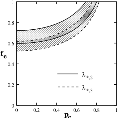
Fig. 7.: Allowed regions for possible values of the core fraction $f_{c}$ and the partially coherent fraction $p_{c}$ are evaluated on the two standard deviation level from the intercept parameter of the second and the third order BE correlation functions, $\lambda_{2,*}$ and $\lambda_{3,*}$

In the CERN SPS S + Pb reactions, the strength of the two- and three-particle correlation functions was determined experimentally by the NA44 Collaboration as $\lambda_{*,2}=0.44\pm 0.04$ in Ref. [15] and by $\lambda_{*,3}=1.35\pm 0.12\pm 0.09$, Ref. [91]. Note that the value of $\lambda_{*,3}$ was determined with the help of the Coulomb 3-particle wave-function integration method of Ref. [82], reviewed in Section 4, because the estimatebased only on the 3-body Gamow penetration factor introduced unacceptably large systematic errors to the three-particle Bose–Einstein correlation function.

The two experimental values, $\lambda_{*,2}$ and $\lambda_{*,3}$ can be fitted with the two theoretical parameters $f_{c}$ and $p_{c}$, as done in Ref. [86]. Figure 7 illustrates the 2 $\sigma$ contour plots in the $(f_{c},p_{c})$ plane, obtained using the published value of $\lambda_{*,2}=0.44\pm 0.04$ and the preliminary value of $\lambda_{*,3}=1.35\pm 0.12$. A range of $(f_{c},p_{c})$ values is found to describe simultaneously the strength of the two-particle and the three-particle correlation functions within two standard deviations from these values. Thus neither the fully chaotic, nor the partially coherent source picture can be excluded at this level of precision.

Table 2.: Strength of higher-order correlation functions for various core fractions and partially coherent fractions allowed by NA44 2- and 3-particle correlation data

$f_{c}$	$p_{c}$	$\lambda_{*,2}$	$\lambda_{*,3}$	$\lambda_{*,4}$	$\lambda_{*,5}$
0.60	0.00	0.36	1.51	5.05	17.17
0.70	0.50	0.37	1.45	4.25	11.87
1.00	0.75	0.44	1.63	4.33	10.47

Cramer and Kadija pointed out, that for higher values of $n$ the difference between a partially coherent source and between the fully incoherent particle source with an unresolvable component (halo or mis-identified particles) will become larger and larger [92]. Indeed, similar values can be obtained for the strength of the second and third order correlation function, if the source is assumed to be fully incoherent $(f_{c}=0.6,p_{c}=0)$ or if the source has no halo but a partially coherent component $(f_{c}=1,p_{c}=0.75)$, but the strength of the 5th order correlation function is almost a factor of 2 larger in the former case, as can be seen from Table 2. Precision measurements of 4th and 5th order correlations are necessary to determine the value of the degree of partial coherence in the pion source.

6 Particle Interferometry in e${}^{+}+$ e^- Reactions

The hadronic production in e⁺e^- annihilations is usually considered to be a basically coherent process and therefore no Bose–Einstein effect was expected, whereas hadronic reactions should be of a more chaotic nature giving rise to a sizable effect. It was even argued that the strong ordering in rapidity, preventing neighboring $\pi^{-}\pi^{-}$ or $\pi^{+}\pi^{+}$ pairs, would drastically reduce the effect [93]. Therefore it was a surprise when G. Goldhaber at the Lisbon Conference in 1981 [94] presented data which showed that correlations between identical particles in e⁺e^- annihilations were very similar in size and shape to those seen in hadronic reactions, see the review paper Ref. [89] for further details.

6.1 The Andersson–Hofmann model

The Bose–Einstein correlation effect, a priori unexpected for a coherent process, has been given an explanation within the Lund string model by B. Andersson and W. Hofmann [95]. The space-time structure of an e⁺e^- annihilation is shown for the Lund string model [96] in Fig. 8. The probability for a particular final state is given by the expression

$${\rm Prob.}\sim{\rm phasespace}\cdot\exp(-bA),$$ (72)

where $A$ is the space-time area spanned by the string before it breaks and $b$ is a parameter. The classical string action is given by $S=\kappa A$, where $\kappa$ is the string tension. It is natural to interpret the result in Eq. (72) as resulting from an imaginary part of the action such that

$$S=(\kappa+ib/2)A,$$ (73)

and an amplitude $M$ given by

$$M\sim\exp(iS),$$ (74)

which implies

$${\rm Prob.}\sim\mid M\mid^{2}\sim\exp(-bA).$$ (75)

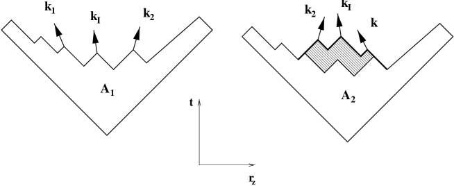
Fig. 8.: Andersson–Hofmann interpretation of Bose–Einstein correlations in the Lund string model. $A_{1,2}$ denotes the space-time area of a color field enclosed by the quark loop in e⁺e^- annihilation. Two particles 1 and 2 are separated by the intermediate system $I$. When the particles 1 and 2 are identical, the configuration in the left side is indistinguishable from that of the right side, and their amplitudes for production must be added. The probability of production will depend on the difference in area $\Delta A=A_{1}-A_{2}$, shown as the hatched area.

Final states with two identical particles are indistinguishable and can be obtained in different ways. Suppose that the two particles indicated as 1 and 2 in Fig. 8 are identical, then the hadron state in the left panel can be considered as being the same as that in the right panel (where 1 and 2 are interchanged). The amplitude should, for bosons, be the sum of two terms

$$M\sim\exp[i(\kappa+ib/2)A_{1}]+\exp[i(\kappa+ib/2)A_{2}]\,,$$ (76)

where $A_{1}$ and $A_{2}$ are the two string areas, giving a probability proportional to

$$\mid M\mid^{2}\sim[\exp(-bA_{1})+\exp(-bA_{2})]\cdot\left[1+{\cos(\kappa\Delta A)\over\cosh(b\Delta A/2)}\right]$$ (77)

with $\Delta A\equiv A_{1}-A_{2}$. The magnitudes of $\kappa$ and $b$ are known from phenomenological studies. The energy per unit length of the string is given by $\kappa\approx 1$ GeV/fm, and $b$ describes the breaking of the string at a constant rate per unit area, $b/\kappa^{2}\approx 0.7$ GeV^-2 [96]. The difference in space-time area $\Delta A$ is marked as the hatched area in Fig. 8. It can be expressed by the $(t,r_{z})$ components $(E,k)$ of the four-momenta of the two identical particles 1 and 2, and the intermediate system $I$:

$$\Delta A=[E_{2}k_{1}-E_{1}k_{2}+E_{I}(k_{1}-k_{2})-k_{I}(E_{1}-E_{2})]/\kappa^{2}\,.$$ (78)

To take into account also the component transverse to the string a small additional term is needed. The change in area $\Delta A$ is Lorentz invariant to boosts along the string direction and is furthermore approximately proportional to $Q=\sqrt{-(k_{1}-k_{2})^{2}}$.

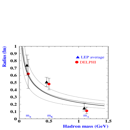
Fig. 9.: Mass dependence of the length of homogeneity in e⁺e^- annihilation at LEP

The interference pattern between the amplitudes will be dominated by the phase change of $\Delta\Phi=\kappa\Delta A$. It leads to a Bose–Einstein correlation which, as a function of the four-momentum transfer, reproduces the data well but shows a steeper dependence at small $Q$ than a Gaussian function. A comparison to TPC data confirmed the existence of such a steeper than Gaussian dependence on $Q$, although the statistics at the small $Q$-values did not allow a firm conclusion [89, 97].

Recently, the interest for multi-dimensional analysis of Bose–Einstein correlations increased also in the particle physics community, see Ref. [66] for a critical review of the present status.

I would like to highlight three interesting features: i) The effect seems to depend on the transverse momentum of the produced pion pairs, decreasing effective radii were observed for increasing transverse mass [51, 52]. This effect is also seen in the LUBOEI algorithm of JETSET, although no intrinsic momentum-dependent scale is plugged into the algorithm [98]. ii) The three-dimensional Bose–Einstein correlations of L3 indicate a non-Gaussian structure [52]. iii) The effective source sizes of heavier particles (K, $\Lambda$) were measured recently [99], based on spin statistics developed by Alexander and Lipkin [100]. The measured source sizes show a clear decrease with increasing particle masses. The latter effect was explained by Alexander, Cohen and Levin [101] by arguments based on the Heisenberg uncertainty relation, and independently with the help of virial theorem applied for a QCD motivated confining potential. See Fig. 9, reproduced from Ref. [102]. Note that a similar decrease was predicted in Ref. [103], which would depend not on the mass, but on the transverse mass of the particles, if the particle production happens so that the position of the emission is very strongly correlated with the momentum of the emitted particle [103]. So, it would be timely to check whether the effect depends on the particle mass, or on the transverse mass. Although the side radius components indicate such a decrease in case of pions, similar measurements for kaons and $\Lambda$-s would be indispensable to clarify the origin of the observed behavior.

The question arises: can the effects i)–iii) be explained in a unified framework, that characterizes the hadronization process in e⁺e^- annihilation? An explanation of the rather small effective size of the source of the $\Lambda$-s seems to be a challenge for the Lund string model.

The three-dimensional analysis of the NA22 data on h + p reactions indicated a strong decrease of all the characteristic radii with increasing values of transverse momenta of the pair in the NA22 experiment [49]. A decrease of the effective source sizes with increasing values of the transverse mass for a given kind of particle is seen in heavy ion collisions, similarly to effect i) in particle physics. The property iii), the decrease of the effective source size with the increase of the mass of the particle is seen in heavy ion physics and is explained in terms of hydrodynamical expansion, similarly to the explanation of effect i), see Figs 15 and 16 in Section 12. Can one give a unified explanation of these similarities between results of particle interferometry in e${}^{+}+$ e^-, h + p and heavy ion physics? We do not yet know the answer to this question.

7 Invariant Buda–Lund Particle Interferometry

The $n$-particle Bose–Einstein correlation function of Eq. (5) is defined as the ratio of the $n$-particle invariant momentum momentum distribution divided by an $n$-fold product of the single-particle invariant momentum distributions. Hence these correlation functions are boost-invariant.

The invariant Buda–Lund parameterization (or BL in short) deals with a boost-invariant, multi-dimensional characterization of the building blocks $\langle a_{{\bf k}_{1}}^{\dagger}a_{{\bf k}_{2}}\rangle$ of arbitrary high order Bose–Einstein correlation functions, based on Eqs (8,13). The BL parameterization was developed by the Buda–Lund Collaboration in Refs [18, 20].

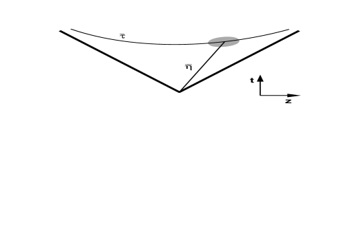
Fig. 10.: Space-time picture of particle emission for a given fixed mean momentum of the pair. The mean value of the proper-time and the space-time rapidity distributions is denoted by ${\overline{\tau}}$ and ${\overline{\eta}}$. As the rapidity of the produced particles changes from the target rapidity to the projectile rapidity the $[{\overline{\tau}}(y),{\overline{\eta}}(y)]$ variables scan the surface of mean particle production in the $(t,r_{z})$ plane.

The essential part of the BL is an invariant decomposition of the relative momentum $q$ in the $\exp(iq\cdot\Delta x)$ factor into a temporal, a longitudinal and two transverse relative momentum components. This decomposition is obtained with the help of a time-like vector in the coordinate space, that characterizes the center of particle emission in space-time, see Fig. 10.

Although the BL parameterization was introduced in Ref. [18] for high energy heavy ion reactions, it can be used for other physical situations as well, where a dominant direction of an approximate boost-invariant expansion of the particle emitting source can be identified and taken as the longitudinal direction $r_{z}$. For example, such a direction is the thrust axis of single jets or of back-to-back two-jet events in case of high energy particle physics. For longitudinally almost boost-invariant systems, it is advantageous to introduce the boost invariant variable $\tau$ and the space-time rapidity $\eta$,

$$\tau = \sqrt{t^{2}-r_{z}^{2}},$$ (79)

$$\eta = 0.5\log\left[(t+r_{z})/(t-r_{z})\right].$$ (80)

Similarly, in momentum space one introduces the transverse mass $m_{t}$ and the rapidity $y$ as

$$m_{t} = \sqrt{E^{2}-p_{z}^{2}},$$ (81)

$$y = 0.5\log\left[(E+p_{z})/(E-p_{z})\right].$$ (82)

The source of particles is characterized in the boost invariant variables $\tau$, $m_{t}$ and $\eta-y$. For systems that are only approximately boost-invariant, the emission function may also depend on the deviation from mid-rapidity, $y_{0}$. The scale on which the approximate boost-invariance breaks down is denoted by $\Delta\eta$, a parameter that is related to the width of the rapidity distribution.

The correlation function is defined with the help of the Wigner function formalism, Eq. (13), the intercept parameter $\lambda_{*}$ is introduced in the core/halo picture of Eq. (42). The case of $n=2$ particles and a chaotic core with $p_{c}=0$ was discussed in Ref. [18]. In the following, we evaluate the building block for arbitrary high order Bose–Einstein correlation functions. We assume for simplicity that the core is fully incoherent, $p_{c}(j)=0$ in Eq. (63). A further simplification is obtained if we assume that the emission function of Eqs (13,42) factorizes as a product of an effective proper-time distribution, a space-time rapidity distribution and a transverse coordinate distribution [104, 18]:

$$S_{c}(x,K)d^{4}x = H_{*}(\tau)G_{*}(\eta)I_{*}(r_{x},r_{y})\,d\tau\,{\overline{\tau}}d\eta dr_{x}dr_{y}.$$ (83)

The subscript $*$ stands for a dependence on the mean momentum $K$, the mid-rapidity $y_{0}$ and the scale of violation of boost-invariance $\Delta\eta$, using the symbolic notation $f_{*}\equiv f[K,y_{0},\Delta\eta]$. The function $H_{*}(\tau)$ stands for such an effective proper-time distribution (that includes, by definition, an extra factor $\tau$ from the Jacobian $d^{4}x=d\tau\,\tau\,d\eta,dr_{x}dr_{y}$, in order to relate the two-particle Bose–Einstein correlation function to a Fourier transformation of a distribution function in $\tau$). The effective space-time rapidity distribution is denoted by $G_{*}(\eta)$, while the effective transverse distribution is denoted by $I_{*}(r_{x},r_{y})$. In Eq. (83), the mean value of the proper-time ${\overline{\tau}}$ is factored out, to keep the distribution functions dimensionless. Such a pattern of particle production is visualized in Fig. 10.

In case of hydrodynamical models, as well as in case of a decaying Lund strings [104, 20], production of particles with a given momentum rapidity $y$ is limited to a narrow region in space-time around ${\overline{\eta}}$ and ${\overline{\tau}}$. If the sizes of the effective source are sufficiently small (if the Bose–Einstein correlation function is sufficiently broad), the $\exp(iq\cdot\Delta x)$ factor of the Fourier transformation is decomposed in the shaded region in Fig. 10 as

$$\exp[i(q^{0}\Delta t-q_{z}\Delta r_{z})] \simeq \exp[i(Q_{=}\Delta\tau-Q_{\parallel}{\overline{\tau}}\Delta\eta)],$$ (84)

$$\exp[-i(q_{x}\Delta r_{x}+iq_{y}\Delta r_{y})] \equiv \exp[-i(Q_{:}\Delta r_{:}+Q_{..}\Delta r_{..})].$$ (85)

The invariant temporal, parallel, sideward, outward (and perpendicular) relative momentum components are defined, respectively, as

$$Q_{=} = q_{0}\cosh[{\overline{\eta}}]-q_{z}\sinh[{\overline{\eta}}],$$ (86)

$$Q_{\parallel} = q_{z}\cosh[{\overline{\eta}}]-q_{0}\sinh[{\overline{\eta}}],$$ (87)

$$Q_{..} = (q_{x}K_{y}-q_{y}K_{x})/\sqrt{K_{x}^{2}+K_{y}^{2}},$$ (88)

$$Q_{:} = (q_{x}K_{x}+q_{y}K_{y})/\sqrt{K_{x}^{2}+K_{y}^{2}},$$ (89)

$$Q_{\perp} = \sqrt{q_{x}^{2}+q_{y}^{2}}=\sqrt{Q_{:}^{2}+Q_{..}^{2}}.$$ (90)

The time-like normal-vector ${\overline{n}}$ indicates an invariant direction of the source in coordinate space [18]. It is parameterized as ${\overline{n}}^{\mu}=(\cosh[{\overline{\eta}}],0,0,\sinh[{\overline{\eta}}])$, where ${\overline{\eta}}$ is a mean space-time rapidity [18, 27, 20]. The parameter ${\overline{\eta}}$ is one of the fitted parameters in the BL type of decomposition of the relative momenta. The above equations are invariant, they can be evaluated in any frame. To simplify the presentation, in the following we evaluate $q$ and ${\overline{\eta}}$ in the LCMS. The acronym LCMS stands for the Longitudinal Center of Mass System, where the mean momentum of a particle pair has vanishing longitudinal component, $K_{z}=0.5(k_{1,z}+k_{2,z})=0.$ In this frame, introduced in Ref. [104], ${\bf K}$ is orthogonal to the beam axis, and the time-like information on the duration of the particle emission couples to the out direction. The rapidity of the LCMS frame can be easily found from the measurement of the momentum vectors of the particles. As ${\overline{\eta}}$ is from now on a space-time rapidity measured in the LCMS frame, it is invariant to longitudinal boosts: ${\overline{\eta}}^{\prime}=({\overline{\eta}}-y)-(0-y)={\overline{\eta}}$.

The symbolic notation for the side direction is two dots side by side as in $Q_{..}$. The remaining transverse direction, the out direction was indexed as in $Q_{:}$, in an attempt to help to distinguish the zeroth component of the relative momentum $Q_{0}$ from the out component of the relative momentum $Q_{:}\equiv Q_{o}=Q_{\rm out}$, $Q_{0}\neq Q_{o}$. Hence $K_{:}=|{\bf K}_{\perp}|$ and $K_{..}=0$. The geometrical idea behind this notation is explained in details in Ref. [27].

The perpendicular (or transverse) component of the relative momentum is denoted by $Q_{\perp}$. By definition, $Q_{..}$, $Q_{:}$ and $Q_{\perp}$ are invariants to longitudinal boosts, and $Q^{2}=-q\cdot q=Q_{..}^{2}+Q_{:}^{2}+Q_{||}^{2}-Q_{=}^{2}$.

With the help of the small source size (or large relative momentum) expansion of Eq. (84), the amplitude $\tilde{s}_{c}(1,2)=\tilde{s}_{c}^{i}(1,2)$ that determines the arbitrary order Bose–Einstein correlation functions in Eq. (63) can be written as follows:

$$\tilde{s}^{i}_{c}(1,2)=\frac{\tilde{H}_{*}(Q_{=})\tilde{G}_{*}(Q_{\parallel})\tilde{I}_{*}(Q_{:},\,Q_{..})}{\tilde{H}_{*}(0)\tilde{G}_{*}(0)\tilde{I}_{*}(0,0)}.$$ (91)

This expression and Eq. (63) yield a general, invariant, multi-dimensional Buda–Lund parameterization of order $n$ Bose–Einstein correlation functions, valid for all $n$. The Fourier-transformed distributions are defined as

$$\tilde{H}_{*}(Q_{=}) = \int_{0}^{\infty}d\tau\exp(iQ_{=}\tau)H_{*}(\tau),$$ (92)

$$\tilde{G}_{*}(Q_{\parallel}) = \int_{-\infty}^{\infty}d\eta\exp(-iQ_{\parallel}{\overline{\tau}}\eta)G_{*}(\eta),$$ (93)

$$\tilde{I}_{*}(Q_{:},Q_{..}) = \int_{-\infty}^{\infty}dr_{:}\int_{-\infty}^{\infty}dr_{..}\exp(-iQ_{:}r_{:}-iQ_{..}r_{..})I_{*}(r_{:},r_{..}).$$ (94)

As a particular case of Eqs (91,63) for $n=2$ and $p_{c}(j)=0$, the two-particle BECF can be written into a factorized Buda–Lund form as

$$C({\bf k}_{1},{\bf k}_{2}) = 1+\lambda_{*}(K){\displaystyle\phantom{|}|\tilde{H}_{*}(Q_{=})|^{2}\over\displaystyle|\tilde{H}_{*}(0)|^{2}}\,{\displaystyle\phantom{|}|\tilde{G}_{*}(Q_{\parallel})|^{2}\over\displaystyle|\tilde{G}_{*}(0)|^{2}}\,{\displaystyle\phantom{|}|\tilde{I}_{*}(Q_{:},\,Q_{..})|^{2}\over\displaystyle|\tilde{I}_{*}(0,0)|^{2}}.$$ (95)

Thus, the BL results are rather generic. For example, BL parameterization may in particular limiting cases yield the power-law, the exponential, the double-Gaussian, the Gaussian, or the less familiar oscillating forms of Eq. (128), see also Ref. [27]. The Edgeworth, the Laguerre or other similarly constructed low-momentum expansions [65] can be applied to any of the factors of one variable in Eq. (95) to characterize these unknown shapes in a really model-independent manner, relying only on the convergence properties of expansions in terms of complete orthonormal sets of functions [65].

In a Gaussian approximation and assuming that $R_{:}=R_{..}=R_{\perp}$, the Buda–Lund form of the Bose–Einstein correlation function reads as follows:

$${C_{2}({\bf k}_{1},{\bf k}_{2})=}{1}{+}\lambda_{*}\,{\exp\left(-R^{2}_{=}Q^{2}_{=}-R^{2}_{\parallel}Q^{2}_{\parallel}-R_{\perp}^{2}Q_{\perp}^{2}\right)},$$ (96)

where the 5 fit parameters are $\lambda_{*}$, $R_{=}$, $R_{\parallel}$, $R_{\perp}$ and the value of ${\overline{\eta}}$ that enters the definitions of $Q_{=}$ and $Q_{\parallel}$ in Eqs (86,87). The fit parameter $R_{=}$ reads as $R$-time-like, and this variable measures a width of the proper-time distribution $H_{*}$. The fit parameter $R_{\parallel}$ reads as $R$-parallel, it measures an invariant length parallel to the direction of the expansion. The fit parameter $R_{\perp}$ reads as $R$-perpendicular or $R$-perp. For cylindrically symmetric sources, $R_{\perp}$ measures a transversal rms radius of the particle emitting source.

The BL radius parameters characterize the lengths of homogeneity [105] in a longitudinally boost-invariant manner. The lengths of homogeneity are generally smaller than the momentum-integrated, total extension of the source, they measure a region in space and time, where particle pairs with a given mean momentum ${\bf K}$ are emitted from.

The following Edgeworth expansion can be utilized to characterize non-Gaussian multidimensional Bose–Einstein correlation functions, in a longitudinally boost-invariant manner:

$$C_{2}({\bf k}_{1},{\bf k}_{2}) = 1+\lambda_{E}\exp(-Q_{=}^{2}R_{=}^{2}-Q_{||}^{2}R_{||}^{2}-Q_{\perp}^{2}R_{\perp}^{2})\times$$ (97)

$$\left[1+\frac{\kappa_{3=}}{3!}H_{3}(\sqrt{2}Q_{=}R_{=})+\frac{\kappa_{4=}}{4!}H_{4}(\sqrt{2}Q_{=}R_{=})+...\right]\times$$

$$\left[1+\frac{\kappa_{3||}}{3!}H_{3}(\sqrt{2}Q_{||}R_{||})+\frac{\kappa_{4||}}{4!}H_{4}(\sqrt{2}Q_{||}R_{||})+...\right]\times$$

$$\left[1+\frac{\kappa_{3\perp}}{3!}H_{3}(\sqrt{2}Q_{\perp}R_{\perp})+\frac{\kappa_{4\perp}}{4!}H_{4}(\sqrt{2}Q_{\perp}R_{\perp})+...\right].$$

This yields $5$ free scale parameters for cylindrically symmetric, longitudinally expanding sources, and three series of shape parameters. The scale parameters are $\lambda_{E}$, $R_{=}$, $R_{\parallel}$, $R_{\perp}$ and ${\overline{\eta}}$, that characterize the effective source at a given mean momentum, by giving the vertical scale of the correlations, the invariant temporal, longitudinal and transverse extensions of the source and its invariant direction, which is the space-time rapidity of the effective source in the LCMS frame (the frame where $k_{1,z}+k_{2,z}=0$,  [104]). The three series of shape parameters are $\kappa_{3=}$,$\kappa_{4=}$, … , $\kappa_{3||}$, $\kappa_{4||}$, … , $\kappa_{3\perp}$, $\kappa_{4\perp}$, … . Each of these parameters may depend on the mean momentum ${\bf{K}}$.

A multi-dimensional Laguerre or a mixed Edgeworth–Laguerre expansion can be introduced in a similar manner by replacing the Edgeworth expansion in Eq. (97) by a Laguerre one in any of the principal directions.

In Eqs (97,96), the spatial information about the source distribution in $(r_{x},r_{y})$ was combined to a single perp radius parameter $R_{\perp}$. In a more general Gaussian form, suitable for studying rings of fire and opacity effects, the Buda–Lund  invariant BECF can be denoted as

$$C_{2}({\bf k}_{1},{\bf k}_{2})=1+\lambda_{*}\exp\left(-R_{=}^{2}Q_{=}^{2}-R^{2}_{\parallel}Q^{2}_{\parallel}-R_{..}^{2}Q_{..}^{2}-R_{:}^{2}Q_{:}^{2}\right).$$ (98)

The 6 fit parameters are $\lambda_{*}$, $R_{=}$, $R_{\parallel}$, $R_{..}$, $R_{:}$ and ${\overline{\eta}}$, all are in principle functions of $({\bf K},y_{0},\Delta\eta)$. Note that this equation is identical to Eq. (44) of Ref. [18], rewritten into the new, symbolic notation of the Lorentz-invariant directional decomposition.

The above equation may be relevant for a study of expanding shells, or rings of fire, as discussed first in Ref. [18]. We shall argue, based on a simultaneous analysis of particle spectra and correlations, and on recently found exact solutions of non-relativistic fireball hydrodynamics [39] that an expanding, spherical shell of fire is formed protons in 30 AMeV ⁴⁰Ar + ¹⁹⁷Au reactions, and that a two-dimensional, expanding ring of fire is formed in the transverse plane in NA22 h + p reactions at CERN SPS. The experimental signatures for the formation of these patterns will be discussed in Section 11.

Opacity effects, as suggested recently by H. Heiselberg [106], also require the distinction between $R_{..}$ and $R_{:}$. The lack of transparency in the source may result in an effective source function, that looks like a crescent in the side-out reference frame [106]. When integrated over the direction of the mean momentum, the effective source looks like a ring of fire in the $(r_{x},r_{y})$ frame.

The price of the invariant decomposition of the basic building blocks of any order Bose–Einstein correlation functions in the BL parameterization is that the correlation functions cannot be directly binned in the BL variables, as these can determined after the parameter ${\overline{\eta}}$ is fitted to the data — so the correlation function has to be binned first in some directly measurable relative momentum components, e.g. the (side, out, long) relative momenta in the LCMS frame, as discussed in the next subsection. After fitting ${\overline{\eta}}$ in an arbitrary frame, the BECF can be re-binned into the BL form.

7.1 Gaussian parameterizations of BE Correlations

We briefly summarize here the Bertsch–Pratt and the Yano–Koonin parameterization of the Bose–Einstein correlation functions, to point out some of their advantages as well as drawbacks and to form a basis for comparison.

7.1.1 The Bertsch–Pratt parameterization

The Bertsch–Pratt (BP) parameterization of Bose–Einstein correlation functions is one of the oldest, widely used multi-dimensional decomposition, called also as the side–out–longitudinal decomposition [48, 87].

This directional decomposition was devised to extract the contribution of a long duration of particle emission from an evaporating Quark–Gluon Plasma, as expected in the mixture of a hadronic and a QGP phase if the re-hadronization phase transition is a strong first order transition.

The BP parameterization in a compact form reads as

$$C_{2}({\bf k}_{1},{\bf k}_{2}) = 1+\lambda\exp\left[-R_{s}^{2}Q_{s}^{2}-R_{o}^{2}Q_{o}^{2}-R_{l}^{2}Q_{l}^{2}-2R_{ol}^{2}Q_{l}Q_{o}\right].$$ (99)

Here index $o$ stands for out (and not the temporal direction), $s$ for side and $l$ for longitudinal. The out–longitudinal cross-term was introduced by Chapman, Scotto and Heinz in Refs [22, 23] — this term is non-vanishing for axially symmetric systems, if the source is not fully boost-invariant, or if the measurement is made not at mid-rapidity. In a more detailed form, the mean momentum dependence of the various components is shown as

$$C_{2}({\bf k}_{1},{\bf k}_{2}) = 1+\lambda({\bf K})\exp\left[-R_{s}^{2}({\bf K})Q_{s}^{2}({\bf K})-R_{o}^{2}({\bf K})Q_{o}^{2}({\bf K})\right.$$ (100)

$$\hskip 56.9055pt\left.-R_{l}^{2}({\bf K})Q_{l}^{2}-2R_{ol}^{2}({\bf K})Q_{l}Q_{o}({\bf K})\right]\,,$$

where the mean and the relative momenta are defined as

$${\bf K} = 0.5({\bf k}_{1}+{\bf k}_{2}),$$ (101)

$${\bf\Delta k} = {\bf k}_{1}-{\bf k}_{2},$$ (102)

$$Q_{l} = k_{z,1}-k_{z,2},$$ (103)

$$Q_{o} = Q_{o}({\bf K})\,=\,{\bf\Delta k}\cdot{\bf K}/|{\bf K}|,$$ (104)

$$Q_{s} = Q_{s}({\bf K})\,=\,|{\bf\Delta k}\times{\bf K}|/|{\bf K}|.$$ (105)

It is emphasized that the BP radius parameters are also measuring lengths of homogeneity [105]. Not only the radius parameters but also the decomposition of the relative momentum to the side and the out components depends on the (direction of) mean momentum ${\bf K}$.

In an arbitrary frame, Gaussian radius parameters can be defined, and sometimes they are also referred to as BP radii, when the spatial components of the relative momentum vector are taken as independent variables. The BP radii reflect space-time variances [22, 23] of the core [78] of the particle emission, if a Gaussian approximation to the core is warranted:

$$C_{2}({\bf k}_{1},{\bf k}_{2}) = 1+\lambda_{*}({\bf K})\,\exp\left(-R^{2}_{i,j}({\bf K}){\bf\Delta k}_{i}{\bf\Delta k}_{j}\right),$$ (106)

$$\lambda_{*}({\bf K}) = [N_{\bf c}({\bf K})/N({\bf K})]^{2},$$ (107)

$$R_{i,j}^{2}({\bf K}) = \langle\underline{x}_{i}\underline{x}_{j}\rangle_{\bf c}-\langle\underline{x}_{i}\rangle_{\bf c}\langle\underline{x}_{j}\rangle_{\bf c},$$ (108)

$$\underline{x}_{i} = x_{i}-\beta_{i}t,$$ (109)

$$\langle f(x,{\bf k})\rangle_{\bf c} = \int d^{4}xf(x,{\bf k})S_{\bf c}(x,{\bf k})/\int d^{4}xS_{\bf c}(x,{\bf k}),$$ (110)

where $S_{\bf c}(x,{\bf k})$ is the emission function that characterizes the central core and subscripts $i$ or $j$ stand for $x$, $y$ or $z$, i.e. any of the spatial directions in the frame of the analysis. This method is frequently called as “model-independent” formulation, because the applied Gaussian approximation is independent of the functional form of the emission function $S_{(}x,{\bf k})$ [13]. In the literature, this result is often over-stated, it is claimed that such a Taylor expansion would provide a general “proof” that multi-dimensional Bose–Einstein correlation functions must be Gaussians. Although the “proof” is indeed not depending on the exact shape of $S(x,K)$, it relies on a second order Taylor expansion of the shape of the correlation function around its exact value at $Q=0$. At this point not only the derivatives of the correlation function are unmeasurable, but the very value of the correlation function $C_{2}(0)$ is unmeasurable as well, see Figs 4 and 3 for graphical illustration. For exponential or for power-law type correlations, the building block $\tilde{S}_{c}(q,K)$ of the correlation function is not analytic at $Q=0$, so a Taylor expansion cannot be applied in their case. For the oscillatory type of correlation functions, the Gaussian provides a good approximation in the experimentally unresolvable low $Q$ domain, but it misses the structure of oscillations at large values of $Q$, which appear because $S(x,K)$ has more than one maxima, like a source distribution of a binary star. Thus, the exact shapes of multi-dimensional BECF-s cannot be determined a priori and in case of non-Gaussian correlators one has to evaluate more (but still not fully) model-independent relationships, for example Eqs (13,63,91), which are valid for broader than Gaussian classes of correlation functions.

Note that the tails of the emission function are typically dominated by the halo of long-lived resonances $S_{h}(x,{\bf k})$ and even a small admixture of e.g. $\eta$ and $\eta^{\prime}$ mesons increases drastically the space-time variances of particle production, and makes the interpretation of the BP radii in terms of space-time variances of the total emission function $S=S_{c}+S_{h}$ unreliable both qualitatively and quantitatively, as pointed out already in Ref. [78].

In the Longitudinal Center of Mass System (LCMS, Ref. [104]), the BP radii have a particularly simple form [104], if the coupling between the $r_{x}$ and the $t$ coordinates is also negligible, $\langle\tilde{r}_{x}\tilde{t}\rangle=\langle\tilde{r}_{x}\rangle\langle\tilde{t}\rangle$:

$$R_{s}^{2}({\bf K}) = \langle\tilde{r}_{y}^{2}\rangle_{\bf c}\,,$$ (111)

$$R_{o}^{2}({\bf K}) = \langle\tilde{r}_{x}^{2}\rangle_{\bf c}+\beta_{t}^{2}\langle\tilde{t}^{2}\rangle_{\bf c}\,,$$ (112)

$$R_{l}^{2}({\bf K}) = \langle\tilde{r}_{z}^{2}\rangle_{\bf c}\,,$$ (113)

$$R_{ol}^{2}({\bf K}) = \langle\tilde{r}_{z}(\tilde{r}_{x}-\beta_{t}\tilde{t})\rangle_{\bf c}\,,$$ (114)

where $\tilde{x}=x-\langle x\rangle$. Although this method cannot be applied to characterize non-Gaussian correlation functions, the the above form has a number of advantages:it is straightforward to obtain and it is easy to implement for a numerical evaluation of the BP radii of Gaussian correlation functions [13].

In the LCMS frame, information on the duration of the particle emission couples only to the out direction. This is one of the advantages of the LCMS frame. Using the BP, the time distribution enters the out radius component as well as the out-long cross-term. Other possible cross-terms were shown to vanish for cylindrically symmetric sources [22, 23].

For completeness, we give the relationship between the invariant BL radii and the BP radii measured in the LCMS, if the BL forms are given in the Gaussian approximation of Eq. (98):

$$R_{s}^{2} = R_{..}^{2},$$ (115)

$$R_{o}^{2} = R_{:}^{2}+\beta_{t}^{2}[\cosh^{2}({\overline{\eta}})R_{=}^{2}+\sinh^{2}({\overline{\eta}})R_{\parallel}^{2}],$$ (116)

$$R_{ol}^{2} = -\beta_{t}\sinh({\overline{\eta}})\cosh({\overline{\eta}})(R_{=}^{2}+R_{\parallel}^{2}),$$ (117)

$$R_{l}^{2} = \cosh^{2}({\overline{\eta}})R_{\parallel}^{2}+\sinh^{2}({\overline{\eta}})R_{=}^{2},$$ (118)

where the dependence of the fit parameters on the value of the mean momentum, ${\bf K}$ is suppressed. The advantage of the BP parameterization is that there are no kinematic constraints between the side, out and long components of the relative momenta, hence the BP radii are not too difficult to determine experimentally. A drawback is that the BP radii are not invariant, they depend on the frame where they are evaluated. The BP radii transform as a well-defined mixture of the invariant temporal, longitudinal and transverse BL radii, given e.g. in Ref. [18].

7.1.2 The Yano–Koonin–Podgoretskii parameterization

A covariant parameterization of two-particle correlations has been worked out for non-expanding sources by Yano, Koonin and Podgoretskii (YKP) [107, 108]. This parameterization was recently applied to expanding sources by the Regensburg group [109, 110], by allowing the YKP radius and velocity parameters be momentum dependent:

$$C_{2}({\bf k}_{1},{\bf k}_{2}) = 1+\exp\left[-R_{\perp}^{2}({\bf K})q_{\perp}^{2}-R_{\parallel}^{2}({\bf K})(q_{z}^{2}-q_{0}^{2})\right.$$ (119)

$$\hskip 56.9055pt\left.-\left(R_{0}^{2}({\bf K})+R_{\parallel}^{2}({\bf K})\right)\left(q\cdot U({\bf K})\right)^{2}\right],$$

where the fit parameter $U({\bf K})$ is interpreted [109, 110] as a four-velocity of a fluid-element [111]. (Note that in YKP index $0$ refers to the time-like components). This generalized YKP parameterization was introduced to create a diagonal Gaussian form in the “rest frame of a fluid-element”.

This form has an advantage as compared to the BP parameterization: the three extracted YKP radius parameters, $R_{\perp}$, $R_{\parallel}$ and $R_{0}$ are invariant, independent of the frame where the analysis is performed, while $U^{\mu}$ transforms as a four-vector. The price one has to pay for this advantage is that the kinematic region may become rather small in the $q_{0}$, $q_{l}$, $q_{\perp}$ space, where the parameters are to be fitted, as follows from the inequalities $Q^{2}=-q\cdot q\geq 0$ and $q^{2}_{0}\geq 0$:

$$0\leq q_{0}^{2}\leq q_{z}^{2}+q_{\perp}^{2},$$ (120)

and the narrowing of the regions in $q^{2}_{0}-q_{z}^{2}$ with decreasing $q_{\perp}$ makes the experimental determination of the YKP parameters difficult, especially when the analysis is performed far from the LCMS rapidities [or more precisely from the frame where $U^{\mu}=(1,0,0,0)$ ].

Theoretical problems with the YKP parameterization are explained as follows. a) The YKP radii contain components proportional to ${1/\beta_{t}}$, which lead to divergent terms for particles with very low $p_{t}$ [109, 110]. b) The YKP fit parameters are not even defined for all Gaussian sources [109, 110]. Especially, for opaque sources, for expanding shells, or for rings of fire with $\langle\tilde{r}_{x}^{2}\rangle<\langle\tilde{r}_{y}^{2}\rangle$ the algebraic relations defining the YKP “velocity” parameter become ill-defined and result in imaginary values of the YKP “velocity”, [109, 110]. c) The YKP “flow velocity” $U^{\mu}({\bf K})$ is defined in terms of space-time variances at fixed mean momentum of the particle pairs [109, 110], corresponding to a weighted average of particle coordinates. In contrast, the local flow velocity $u^{\mu}(x)$ is defined as a local average of particle momenta. Hence, in general $U^{\mu}({\bf{K}})\neq u^{\mu}(x)$, and the interpretation of the YKP parameter $U^{\mu}({\bf K})$ as a local flow velocity of a fluid does not correspond to the principles of kinetic theory.

8 Hydrodynamical Parameterization à la Buda–Lund (BL-H)

The Buda–Lund hydro parameterization (BL-H) was invented in the same paper as the BL parameterization of the Bose–Einstein correlation functions [18], but in principle the general BL forms of the correlation function do not depend on the hydrodynamical ansatz (BL-H). The BL form of the correlation function can be evaluated for any, non-thermalized expanding sources, e.g.  for the Lund string model also.

The BL-H assumes, that the core emission function is characterized with a locally thermalized, volume-emitting source:

$$S_{c}(x,{\bf k})\,d^{4}x = {\displaystyle\phantom{|}g\over\displaystyle(2\pi)^{3}}\,\,{k^{\mu}d^{4}\Sigma_{\mu}(x)\over\displaystyle\exp\left({\displaystyle\phantom{|}u^{\mu}(x)k_{\mu}\over\displaystyle T(x)}-{\displaystyle\phantom{|}\mu(x)\over\displaystyle T(x)}\right)+s}.$$ (121)

The degeneracy factor is denoted by $g$, the four-velocity field is denoted by $u^{\mu}(x)$, the temperature field is denoted by $T(x)$, the chemical potential distribution by $\mu(x)$ and $s=0$, $-1$ or $1$ for Boltzmann, Bose–Einstein or Fermi–Dirac statistics. The particle flux over the freeze-out layers is given by a generalized Cooper–Frye factor, assuming that the freeze-out hypersurface depends parametrically on the freeze-out time $\tau$ and that the probability to freeze-out at a certain value is proportional to $H(\tau)$,

$$k^{\mu}d^{4}\Sigma_{\mu}(x) = m_{t}\cosh[\eta-y]H(\tau)d\tau\,{\overline{\tau}}d\eta\,dr_{x}\,dr_{y}.$$ (122)

The four-velocity $u^{\mu}(x)$ of the expanding matter is assumed to be a scaling longitudinal Bjorken flow appended with a linear transverse flow, characterized by its mean value $\langle u_{t}\rangle$, see Refs [18, 23, 29]:

$$u^{\mu}(x) = \left(\cosh[\eta]\cosh[\eta_{t}],\,\sinh[\eta_{t}]\frac{r_{x}}{r_{t}},\,\sinh[\eta_{t}]\frac{r_{y}}{r_{t}},\,\sinh[\eta]\cosh[\eta_{t}]\right),$$

$$\sinh[\eta_{t}] = \langle u_{t}\rangle r_{t}/R_{G},$$ (123)

with $r_{t}=[r_{x}^{2}+r_{y}^{2}]^{1/2}$. Such a flow profile, with a time-dependent radius parameter $R_{G}$, was recently shown to be an exact solution of the equations of relativistic hydrodynamics of a perfect fluid at a vanishing speed of sound, Ref. [40].

Instead of applying an exact hydrodynamical solution with evaporation terms, the BL-H characterizes the local temperature, flow and chemical potential distributions of a cylindrically symmetric, finite hydrodynamically expanding system with the means and the variances of these distributions. The hydrodynamical variables $1/T(x)$, $\mu(x)/T(x)$, are parameterized as

$${\displaystyle\phantom{|}\mu(x)\over\displaystyle T(x)} = {\displaystyle\phantom{|}\mu_{0}\over\displaystyle T_{0}}-{\displaystyle\phantom{|}r_{x}^{2}+r_{y}^{2}\over\displaystyle 2R_{G}^{2}}-{\displaystyle\phantom{|}(\eta-y_{0})^{2}\over\displaystyle 2\Delta\eta^{2}},$$ (124)

$${\displaystyle\phantom{|}1\over\displaystyle T(x)} = {\displaystyle\phantom{|}1\over\displaystyle T_{0}}\,\,\left(1+\Big{\langle}{\Delta T\over T}\Big{\rangle}_{r}\,{\displaystyle\phantom{|}r_{t}^{2}\over\displaystyle 2R_{G}^{2}}\right)\,\left(1+\Big{\langle}{\Delta T\over T}\Big{\rangle}_{t}\,{\displaystyle\phantom{|}(\tau-\overline{\tau})^{2}\over\displaystyle 2\Delta\tau^{2}}\right),$$ (125)

the temporal distribution of particle evaporation $H(\tau)$ is assumed to have the form of

$$H(\tau)=\frac{1}{(2\pi\Delta\tau^{2})^{3/2}}\exp\left[-\frac{(\tau-{\overline{\tau}})^{2}}{2\Delta\tau^{2}}\right],$$ (126)

and it is assumed that the widths of the particle emitting sources, e.g. $R_{G}$ and $\Delta\eta$ do not change significantly during the course of the emission of the observable particles. The parameters $\langle{\Delta T/T}\rangle_{r}$ and $\langle{\Delta T/T}\rangle_{t}$ control the transversal and the temporal changes of the local temperature profile, see Refs [27, 19, 18] for further details. This formulation of the BL hydro source includes a competition between the transversal flow and the transverse temperature gradient, in an analytically tractable form. In the analytic evaluation of this model, it is assumed that the transverse flow is non-relativistic at the point of maximum emissivity [23], the temperature gradients were introduced following the suggestion of Akkelin and Sinyukov [112].

Note that the shape of the profile function in $\eta$ is assumed to be a Gaussian in Eq. (124) in the spirit of introducing only means and variances. However, in Ref. [17] a formula was given, that allows the reconstruction of this part of the emission function from the measured double-differential invariant momentum distribution in a general manner, for arbitrary sources with scaling longitudinal expansions.

8.1 Correlations and spectra for the BL-Hydro

Using the binary source formulation, reviewed in the next section, the invariant single particle spectrum is obtained as

$$N_{1}({\bf k}) = {\displaystyle\phantom{|}g\over\displaystyle(2\pi)^{3}}\,\overline{E}\,\overline{V}\,\overline{C}\,{1\over\displaystyle\exp\left({\displaystyle\phantom{|}u^{\mu}(\overline{x})k_{\mu}\over\displaystyle T(\overline{x})}-{\displaystyle\phantom{|}\mu(\overline{x})\over\displaystyle T(\overline{x})}\right)+s}.$$ (127)

The two-particle Bose–Einstein correlation function was evaluated in the binary source formalism in Ref. [27]:

$$C_{2}({\bf k}_{1},{\bf k}_{2}) = 1+\lambda_{*}\,\Omega(Q_{\parallel})\,\,\,\exp\left(-Q_{\parallel}^{2}\overline{R}_{\parallel}^{2}-Q_{=}^{2}\overline{R}_{=}^{2}-Q_{\perp}^{2}\overline{R}_{\perp}^{2}\right),$$ (128)

where the pre-factor $\Omega(Q_{\parallel})$ induces oscillations within the Gaussian envelope as a function of $Q_{\parallel}$. This oscillating pre-factor satisfies $0\leq\Omega(Q_{\parallel})\leq 1$ and $\Omega(0)=1$. This factor is given as

$$\Omega(Q_{\parallel}) = \cos^{2}(Q_{\parallel}\overline{R}_{\parallel}\,{\Delta{\overline{\eta}}})+\sin^{2}(Q_{\parallel}\overline{R}_{\parallel}\,{\Delta{\overline{\eta}}})\tanh^{2}({{\overline{\eta}}}).$$ (129)

The invariant BL decomposition of the relative momentum is utilized to present the correlation function in the simplest possible form. Although the shape of the BECF is non-Gaussian, because the factor $\Omega(Q_{\parallel})$ results in oscillations of the correlator, the result is still explicitly boost-invariant. Although the source is assumed to be cylindrically symmetric, we have 6 free fit parameters in this BL form of the correlation function: $\lambda_{*}$, $R_{=}$, $R_{\parallel}$, $R_{\perp}$, ${\overline{\eta}}$ and ${\Delta{\overline{\eta}}}$. The latter controls the period of the oscillations in the correlation function, which in turn carries information on the separation of the effective binary sources. This emphasizes the importance of the oscillating factor in the BL Bose–Einstein correlation function.

The parameters of the spectrum and the correlation function are the same, defined as follows. In the above equations, $\overline{a}$ means a momentum-dependent average of the quantity $a$. The average value of the space-time four-vector $\overline{x}$ is parameterized by $(\overline{\tau},\overline{\eta},\overline{r_{x}},\overline{r_{y}})$, denoting longitudinal proper-time, space-time rapidity and transverse directions. These values are obtained in terms of the BL-H parameters in a linearized solution of the saddle-point equations as

$$\overline{\tau} = \tau_{0},$$ (130)

$$\overline{\eta} = {(y_{0}-y)/\left[1+\Delta\eta^{2}m_{t}/T_{0}\right]},$$ (131)

$$\overline{r_{x}} = \langle u_{t}\rangle R_{G}{\displaystyle\phantom{|}p_{t}\over\displaystyle T_{0}+\overline{E}\left(\langle u_{t}\rangle+\langle{\displaystyle\phantom{|}\Delta T/T}\rangle_{r}\right)},$$ (132)

$$\overline{r_{y}} =0.$$ (133)

In Eq. (127), $\overline{E}$ stands for an average energy, $\overline{V}$ for an average volume of the effective source of particles with a given momentum $k$ and $\overline{C}$ for a correction factor, each defined in the LCMS frame:

$$\overline{E} = m_{t}\cosh(\overline{\eta}),$$ (134)

$${\overline{V}} = (2\pi)^{\frac{3}{2}}\,\overline{R}_{\parallel}\,\,\overline{R}_{\perp}^{2}\,\,{\displaystyle\phantom{|}{\Delta{\overline{\tau}}}\,\over\displaystyle{\Delta\tau}},$$ (135)

$$\overline{C}\, = \exp\left({{\Delta{\overline{\eta}}}^{2}/2}\right)/\sqrt{\lambda_{*}}.$$ (136)

The average invariant volume ${\overline{V}}$ is given as a time-averaged product of the transverse area $\overline{R}_{\perp}$ and the invariant longitudinal source size $\overline{R}_{\parallel}$, given as

$$\overline{R}_{\perp}^{2} = R^{2}_{..}\,=\,R^{2}_{:}\,=\,{R_{G}^{2}/\left[1+\left(\langle u_{t}\rangle^{2}+\langle{{\small\Delta T/T}}\rangle_{r}\right){\overline{E}/T_{0}}\right]},$$ (137)

$$\overline{R}_{\parallel}^{2} = {\overline{\tau}}^{2}\,{\Delta{\overline{\eta}}}^{2},$$ (138)

$${\Delta{\overline{\eta}}}^{2} = {\Delta\eta^{2}/\left(1+\Delta\eta^{2}{\overline{E}/T_{0}}\right)},$$ (139)

$$\overline{R}_{=}^{2} = {\Delta{\overline{\tau}}}^{2}\,=\,{\Delta\tau^{2}/\left(1+\langle{{\small\Delta T/T}}\rangle_{t}{\overline{E}/T_{0}}\right)}.$$ (140)

This completes the specification of the shape of particle spectrum and that of the two-particle Bose–Einstein correlation function. These results for the spectrum correspond to the equations given in Ref. [18] although they are expressed here using an improved notation.

In a generalized form, the thermal scales are defined as the $\overline{E}/T_{0}$ $\rightarrow\infty$ limit of Eqs (137–140), while the geometrical scales correspond to dominant terms in the $\overline{E}/T_{0}\rightarrow 0$ limit of these equations. In all directions, including the temporal one, the length-scales measured by the Bose–Einstein correlation function are dominated by the smaller of the thermal and the geometrical length-scales. As shown in Sections 11 and 12, the width of the rapidity distribution and the slope of the transverse-mass distribution is dominated by the bigger of the geometrical and the thermal length-scales. This is the analytic reason, why the geometrical source sizes, the flow and temperature profiles of the source can only be reconstructed with the help of a simultaneous analysis of the two-particle Bose–Einstein correlation functions and the single-particle momentum distribution  [16, 17, 18, 19, 20].

If the geometrical contributions to the HBT radii are sufficiently large as compared to the thermal scales, they cancel from the measured HBT radius parameters. In this case, even if the geometrical source distribution for different particles (pions, kaons, protons) were different, the HBT radii (lengths of homogeneity) approach a scaling function in the large $\overline{E}/T_{0}$ limit. Up to the leading order calculation in the transverse coordinate of the saddle-point, this model predicts a scaling in terms of $\overline{E}$, which variable coincides with the transverse mass $m_{t}$ at mid-rapidity.Phenomenologically, the scaling law can be summarized as $R_{i}\propto m_{t}^{\alpha_{i}}$, where $i$ indexes the directional dependence, and the exponent $\alpha_{i}$ may be slightly rapidity dependent, due to the difference between $\overline{E}$ and $m_{t}$, and it may phenomenologically reflect the effects of finite size corrections as well. Note also that such a scaling limiting case is only a possibility in the BL-H, valid in certain domain of parameter space, but it is not a necessity. The analysis of Pb + Pb collisions at 158 AGeV indicates that BL-H describes the data fairly well, but the longitudinal radius component exhibits different scaling behavior from the transverse radii, see Section 12 for more details.

9 Binary Source Formalism

Let us first consider the binary source representation of the BL-H model. The two-particle Bose–Einstein correlation function was evaluated in Ref. [18] only in a Gaussian approximation, without applying the binary source formulation. An improved calculation was recently presented in Ref. [27], where the correlation function was evaluated using in the binary source formulation, and the corresponding oscillations were found.

Using the exponential form of the $\cosh[\eta-y]$ factor, the BL-H emission function $S_{c}(x,{\bf k})$ can be written as a sum of two terms:

$$S_{c}(x,{\bf k}) = 0.5\,[S_{+}(x,{\bf k})+S_{-}(x,{\bf k})],$$ (141)

$$S_{\pm}(x,{\bf k}) = \frac{g}{(2\pi)^{3}}m_{t}\exp[\pm\eta\mp y]H_{*}(\tau)\frac{1}{[f_{B}(x,{\bf k})+s]},$$ (142)

$$f_{B}(x,{\bf k}) = \exp\left[\frac{k^{\mu}u_{\mu}(x)-\mu(x)}{T(x)}\right].$$ (143)

Let us call this splitting as the binary source formulation of the BL-H parameterization. The effective emission function components are both subject to Fourier transformation in the BL approach. In an improved saddle-point approximation, the two components $S_{+}(x,k)$ and $S_{-}(x,k)$ can be Fourier-transformed independently, finding the separate maxima (saddle point) ${\overline{x}}_{+}$ and ${\overline{x}}_{-}$ of $S_{+}(x,k)$ and $S_{-}(x,k)$, and performing the analytic calculation for the two components separately.

The oscillations in the correlation function are due to this effective separation of the pion source to two components, a splitting caused by the Cooper–Frye flux term. These oscillations in the intensity correlation function are similar to the oscillations in the intensity correlations of photons from binary stars in stellar astronomy [113].

Due to the analytically found oscillations, the presented form of the BECF goes beyond the single Gaussian version of the saddle-point calculations of Refs [22, 23]. This result goes also beyond the results obtainable in the YKP or the BP parameterizations. In principle, the binary-source saddle-point calculation gives more accurate analytic results than the numerical evaluation of space-time variances, as the binary-source calculation keeps non-Gaussian information on the detailed shape of the Bose–Einstein correlation function.

Note that the oscillations are expected to be small in the BL-H picture, and the Gaussian remains a good approximation to Eq. (128), but with modified radius parameters.

9.1 The general binary source formalism

In the previous subsection, we have seen how effective binary sources appear in the BL-H model in high energy physics. However, binary sources appear generally: in astrophysics, in form of binary stars, in particle physics, in form of W⁺W^- pairs, that separate before they decay to hadrons.

Let us consider first the simplest possible example, to see how the binary sources result in oscillations in the Bose–Einstein or Fermi–Dirac correlation function. Suppose a source distribution $s(x-x_{+})$ describes e.g. a Gaussian source, centered on $x_{+}$. Consider a binary system, where the emission happens from $s_{+}=s(x-x_{+})$ with fraction $f_{+}$, or from a displaced source, $s_{-}=s(x-x_{-})$, centered on $x_{-}$, with a fraction $f_{-}$. For such a binary source, the amplitude of the emission is

$$\rho(x)=f_{+}s(x-x_{+})+f_{-}s(x-x_{-}),$$ (144)

and the normalization requires

$$f_{+}+f_{-}=1\,.$$ (145)

The two-particle Bose–Einstein or Fermi–Dirac correlation function is

$$C(q) = 1\pm|\tilde{\rho}(q)|^{2}=1\pm\Omega(q)|\tilde{s}(q)|^{2},$$ (146)

where $+$ is for bosons, and $-$ for fermions. The oscillating pre-factor $\Omega(q)$ satisfies $0\leq\Omega(q)\leq 1$ and $\Omega(0)=1$. This factor is given as

$$\Omega(q) = \left[(f_{+}^{2}+f_{-}^{2})+2f_{+}f_{-}\cos[q(x_{+}-x_{-})]\right]\,.$$ (147)

The strength of the oscillations is controlled by the relative strength of emission from the displaced sources and the period of the oscillations can be used to learn about the distance of the emitters. In the limit of one emitter ($f_{+}=1$ and $f_{-}=0$, or vice versa), the oscillations disappear.

The oscillating part of the correlation function in high energy physics is expected to be much smaller, than that of binary stars in stellar astronomy. In particle physics, the effective separation between the sources can be estimated from the uncertainty relation to be $x_{\pm}=|x_{+}-x_{-}|\approx 2\hbar/M_{\rm W}\approx 0.005$ fm. Although this is much smaller, the effective size of the pion source, 1 fm, one has to keep in mind that the back-to-back momenta of the W⁺W^- pairs can be large, as compared to the pion mass. Due to this boost, pions with similar momentum may be emitted from different W-s with a separation which is already comparable to the 1 fm hadronization scale, and the resulting oscillations may become observable.

In stellar astronomy, the separation between the binary stars is typically much larger than the diameter of the stars, hence the oscillations are well measurable. In principle, similar oscillations may provide a tool to measure the separation of the W⁺ from W^- in 4-jet events at LEP2. The scale of separation of W⁺W^- pairs is a key observable to estimate in a quantum-mechanically correct manner the influence of the Bose–Einstein correlations on the reconstruction of the W mass.

In heavy ion physics, oscillations are seen in the long-range part of the p + p Fermi–Dirac correlation function [114], with a half-period of $Q_{h}=30$ MeV. This implies a separation of $x_{\pm}=\pi\hbar/Q_{h}\approx 20$ fm, which can be attributed to interference between the the two peaks of the NA49 proton $dn/dy$ distribution [115], separated by $\Delta y=2.5$. As for the protons we have $m\gg T_{0}=140$ MeV, we can identify this rapidity difference with the space-time rapidity difference between the two peaks of the rapidity distribution. The longitudinal scale of the separation is then given by $x_{\pm}=2{\overline{\tau}}\sinh(\Delta\eta_{p}/2)$, which can be used to estimate the mean freeze-out time of protons, ${\overline{\tau}}=\pi\hbar/[2Q_{h}\sinh(\Delta\eta_{p}/2)]\approx 6.4$ fm/c, in a good agreement with the average value of ${\overline{\tau}}=5.9\pm 0.6$ as extracted from the simultaneous analysis of the single-particle spectra and HBT radii in NA44, NA49 and WA98 experiments in the Buda–Lund picture, as summarized in Section 12.

10 Particle Correlations and Spectra at 30 – 160 AMeV

There are important qualitative differences between relativistic heavy ion collisions at CERN SPS and those at non-relativistic energies from the point of view of particle sources. Low and intermediate energy reactions may create a very long-lived, evaporative source, with characteristic lifetimes of a few 100 fm/c, in contrast to the relatively short-lived systems of lifetimes of the order of 10 fm/c at CERN SPS. During such long evaporation times, cooling of the source is unavoidable and has to be included into the model. Furthermore, in the non-relativistic heavy ion collisions mostly protons and neutrons are emitted and they have much stronger final-state interactions than the pions dominating the final state at ultra-relativistic energies, see Refs [116, 117, 118] for recent reviews.

The evolution of the particle emission in a heavy-ion collision at intermediate energies may roughly be described as: production of pre-equilibrium particles; expansion and possible freeze-out of a compound source; possible evaporation from an excited residue of the source. Note though that this separation is not very distinct and there is an overlap between the different stages. The importance of the various stages above also depends on the beam energy and the impact parameter of the collision. See the review paper of Ref. [118] for greater details.

Sophisticated microscopical transport descriptions [119], such as the BUU(Boltzmann–Uehling–Uhlenbeck) and the QMD (Quantum Molecular Dynamics) models are well-known and believed to provide a reasonable picture of proton emission in central heavy ion collisions from a few tenths up to hundreds of MeV per nucleon. However, the BUU model predicts too large correlations and underpredicts the number of protons emitted with low energies, for the reaction ³⁶Ar + ⁴⁵Sc at $E=120$ and 160 MeV/nucleon, see Ref. [120]. This indicates that the simultaneous description of two-particle correlations and single-particle spectra is a rather difficult task. For energies below a few tens of MeV per nucleon, where long-lived evaporative particle emission is expected to dominate, the measured two-protoncorrelation functions were found to be consistent with compound-nucleus model predictions [121].

A simultaneous analysis of proton and neutron single particle spectra and two-particle correlation was presented in Ref. [26]. This model calculation described the second stage above and, for long emission times, also part of the third stage. In Ref. [26], the competition among particle evaporation, temperature gradient and flow was investigated in a phenomenological manner, based on a simultaneous analysis of quantum statistical correlations and momentum distributions for a non-relativistic, spherically symmetric, three-dimensionally expanding, finite source. The model used can be considered as a non-relativistic, spherically symmetric version of the BL-H hydro parameterization [26].

The non-relativistic kinetic energy is denoted by $E_{k}({\bf k})={\bf k}^{\,2}/(2\,m)$. The following result is obtained for the effective source size $R_{*}$:

$${R_{*}^{2}({\bf k})} = \frac{R_{G}^{2}}{1+\left[\langle\Delta T/T\rangle_{r}E_{k}({\bf k})+m\langle u_{t}\rangle^{2}\right]/T_{0}}\,.$$ (148)

The analytic results for the momentum distribution and the quantum statistical correlation function are given in the Boltzmann approximation as

$$N_{1}({\bf k}) = \frac{g}{(2\pi)^{3}}E_{k}({\bf k})V_{*}({\bf k})\exp\left[-\frac{({\bf k}-m{\bf u}({\bf r}_{s}({\bf k}\,)))^{2}}{2mT({\bf r}_{s}({\bf k}\,))}+\frac{\mu({\bf r}_{s}({\bf k}))}{T({\bf r}_{s}({\bf k}))}\right]\ ,$$

$$V_{*}({\bf k}) = \left[2\pi R_{*}^{2}({\bf k}\,)\right]^{3/2}\,,$$ (150)

$$C(K,\Delta k\,) = 1\pm\exp(-R_{*}^{2}({\bf K}){\bf\Delta k}^{2}-\Delta t^{2}\Delta E^{2})\ .$$ (151)

The effects of final-state Coulomb and Yukawa interactions on the two-particle relative wave-functions are neglected in these analytic expressions. When comparing to data, the final-state interactions were taken into account, see Ref. [26] for further details.

These general results for the correlation function indicate structural similarity between the non-relativistic flows in low/intermediate energy heavy ion collisions [16, 26, 39] and the transverse flow effects in relativistic high energy heavy ion and elementary particle induced reactions [19, 20, 18]. The radius parameters of the correlation function and the slopes of the single-particle spectra are momentum dependent both for the non-relativistic versions of the model, presented in Refs [16, 26, 39] and for the model-class with scaling relativistic longitudinal flows, discussed in Refs [18, 19, 20, 27].

Such a momentum-dependent effective source size has been seen in the proton–proton correlation functions in the ²⁷Al (¹⁴N, pp) reactions at $E=75$ MeV/nucleon [117]: the larger the momentum of the protons the smaller the effective source size [117], in qualitative agreement with Eq. (148).

Table 3.: Parameter values obtained from fitting hydro parameters to n and p spectra and correlation functions, as measured by the CHIC Collaboration in 30 AMeV ⁴⁰Ar + ¹⁹⁷Au reactions

	$R_{G}$ (fm)	$T_{0}$ (MeV)	$\langle\Delta T/T\rangle_{r}$	$\langle u\rangle_{t}$
Neutrons	4.0	3.0	0.00	0.018
Protons	4.0	5.0	0.16	0.036

This model was applied in Ref. [26] to the reaction ⁴⁰Ar + ¹⁹⁷Au at 30 MeV/ nucleon. With the parameter set presented in Table 3, we have obtained a simultaneous description of the n and p single particle spectra as well as the nn and pp correlation functions as given by Refs [122, 123, 124]. See Ref. [26] for further details and discussions.

The main effects of the temperature gradient are that it introduces i) a momentum-dependent effective temperature which is decreasing for increasing momentum, resulting in a suppression at high momentum as compared to the Boltzmann distribution; ii) a momentum-dependent effective source size which decreases with increasing total momentum. Agreement with the experimental data is obtained only if the time of duration of the particle emission was rather long, $\langle t\rangle\approx 520$ fm with a variance of $\approx 320$ fm/c.

The obtained parameter set reflects a moderately large system (Gaussian radius parameter $R_{G}$ = 4.0 fm) at a moderate temperature ($T_{0}(n)$ = 3 MeV and $T_{0}(p)$ = 5 MeV) and small flow. The neutrons and the protons seem to have different local temperature distributions: the neutron temperature distribution is homogeneous, while the temperature of the proton source decreases to $T_{s}(p)=4.3$ MeV at the Gaussian radius, a difference that could be attributed to the difference between their Coulomb interactions [26]. An agreement between the model and the data was obtained only if some amount of flow was included [26].

After the completion of the data analysis, a new family of exact solutions of fireball hydrodynamics was found in Ref. [39], which features scaling radial Hubble flow, and an initial inhomogeneous, arbitrary temperature profile. The competition of the temperature gradients and flow effects were shown to lead to the formation of spherical shells of fire in this class of exact hydrodynamical solutions [39], if the temperature gradient was stronger than the flow, $\langle\Delta T/T\rangle_{r}>m\langle u_{t}\rangle^{2}/T_{0}$. This is the case found from the analysis of proton spectra and correlations in Ref. [26], while the neutron data do not satisfy this condition. Assuming the validity of non-relativistic hydrodynamics to characterize this reaction, one finds that a slowly expanding, spherical shell of fire is formed by the protons, while the neutrons remain in a central, slightly colder and even slower expanding, normal fireball in 30 AMeV ⁴⁰Ar + ¹⁹⁷Au heavy ion reactions.

11 Description of h + p Correlations and Spectra at CERN SPS

The invariant spectra of $\pi^{-}$ mesons produced in $(\pi^{+}/{\mathrm{K}}^{+}){\mathrm{p}}$ interactions at 250 GeV/c are analysed in this section in the framework of the BL-H model of three-dimensionally expanding cylindrically symmetric finite systems, following the lines of Ref. [50]. The EHS/NA22 Collaboration has been the first to perform a detailed and combined analysis of single-particle spectra and two-particle Bose–Einstein correlations in high energy physics [50]. NA22 reported a detailed study of multi-dimensional Bose–Einstein correlations, by determining the side, out and the longitudinal radius components at two different values of the mean transversal momenta in $(\pi^{+}/{\mathrm{K}}^{+}){\mathrm{p}}$ at CERN SPS energies [49]. It turned out, however, that the experimental two-particle correlation data were equally well described by a static Kopylov–Podgoretskii parameterization as well as by the predictions of hydrodynamical parameterizations for longitudinally expanding, finite systems. In Refs [18, 19] we have shown, that the combined analysis of two-particle correlations and single-particle spectra may result in a dramatic enhancement of the selective power of data analysis.

The double-differential invariant momentum distribution of Eq. (127) can be substantially simplified for one-dimensional slices [18, 77].

i) At fixed $m_{t}$, the rapidity distribution reduces to

$$N_{1}({\bf k}) = C_{m}\exp\left[-\frac{(y-y_{0})^{2}}{2\Delta y^{2}}\right],$$ (152)

$$\Delta y^{2} = \Delta\eta^{2}+T_{0}/m_{t}\,,$$ (153)

where $C_{m}$ is an $m_{t}$-dependent normalization coefficient and $y_{0}$ is defined above. The width parameter $\Delta y^{2}$ extracted for different $m_{t}$-slices is predicted to depend linearly on $1/m_{t}$, with slope $T_{0}$ and intercept $\Delta\eta^{2}$ . Observe, that this width is dominated by the bigger of the geometrical scale ($\Delta\eta$) and the thermal scale $T_{0}/m_{t}$.

Fig. 11.: The rapidity distributions of centrally produced pions ($|y|<1.5$) for different $m_{t}$-slices given. The curves are the fit results obtained analytically using the BL-H parameterization.

Fig. 12.: The $m_{t}$ distributions of centrally produced pions ($|y|<1.5$) for different $y$-slices given. The curves are the fit results obtained analytically using the BL-H parameterization.

Note that for static fireballs or spherically expanding shells (152) and (153) are satisfied with $\Delta\eta=0$ [77]. Hence the experimental determination of the $1/m_{t}$ dependence of the $\Delta y$ parameter can be utilized to distinguish between longitudinally expanding finite systems versus static fireballs or spherically expanding shells.

ii) At fixed $y$, the $m_{t}^{2}$-distribution reduces to

$$N_{1}({\bf k})=C_{y}m_{t}^{\alpha}\exp\left(-\frac{m_{t}}{T_{{\mathrm{eff}}}}\right)\,,$$ (154)

where $C_{y}$ is a $y$-dependent normalization coefficient and $\alpha$ is related to the effective dimensions of inhomogeneity in the source as $\alpha=1-d_{{\mathrm{eff}}}/2$ [18]. The $y$-dependent “effective temperature” $T_{{\mathrm{eff}}}(y)$ reads as [18]

$$T_{{\mathrm{eff}}}(y)=\frac{T_{*}}{1+a(y-y_{0})^{2}},$$ (155)

where $T_{*}$ is the maximum of $T_{{\mathrm{eff}}}(y)$ achieved at $y=y_{0}$, and parameter $a$ can be expressed with the help of the other fit parameters, see Refs [18, 50].

The slope parameter at mid-rapidity, $T_{*}$ is also determined by an interplay of the central temperature $T_{0}$ the flow effects modeled by $\langle u_{t}\rangle^{2}$ and the temperature difference between the surface and the center, as characterized by $\langle{\Delta T/T}\rangle_{r}$ [18, 29]. Eq. (66) of Ref. [18] can be rewritten as

$$T_{*}=T_{0}+m\langle u_{t}\rangle^{2}\frac{T_{0}}{T_{0}+m\langle{\Delta T\over T}\rangle_{r}}.$$ (156)

The approximations of Eqs (152) and (154) explicitly predict a specific narrowing of the rapidity and transverse-mass spectra with increasing $m_{t}$ and $y$, respectively (cf. (153) and (155)). The character of these variations is expected [77] to be different for the various scenarios of hadron matter evolution. These features of the spectra were found to be in agreement with the NA22 data [50], and were utilized to reconstruct the particle source of h + p reactions in the $(t,r_{z})$ plane.

Table 4.: Fit results to NA22 h+p data at CERN SPS with a Buda–Lund hydro parameterization for $|y|<1.5$

$\alpha$	${\Delta\eta}$	$T_{0}$ (GeV)	$\langle u_{t}\rangle$	$\langle{\Delta T}/{T}\rangle_{r}$	$\chi^{2}$/NDF
$0.26\pm 0.02$	$1.36\pm 0.02$	$0.140\pm 0.003$	$0.20\pm 0.07$	$0.71\pm 0.14$	642/683

11.1 Combination with two-particle correlations

As already mentioned in the introduction, more comprehensive information on geometrical and dynamical properties of the hadron matter evolution are expected from a combined consideration of two-particle correlations and single-particle inclusive spectra  [16, 17, 18, 19, 20, 24, 112].

At mid-rapidity, $y=y_{0}$ and in the LCMS where $k_{1,z}=-k_{2,z}$, the effective BP radii can be approximately expressed form the BL-H parameterization as [18]:

$$R_{l}^{2} = {\overline{\tau}}^{2}\Delta{\overline{\eta}}^{2},$$ (157)

$$R_{o}^{2} = \overline{R}^{2}_{\perp}+\beta_{t}^{2}\Delta{\overline{\tau}}^{2},$$ (158)

$$R_{s}^{2} = \overline{R}^{2}_{\perp}$$ (159)

with

$$\frac{1}{\Delta{\overline{\eta}}^{2}} = \frac{1}{\Delta\eta^{2}}+\frac{M_{t}}{T_{0}}\,,$$ (160)

$$\overline{R}^{2}_{\perp} = \frac{R_{\mathrm{G}}^{2}}{1+\frac{M_{t}}{T_{0}}(\langle u_{t}\rangle^{2}+\langle\frac{\Delta T}{T}\rangle_{r})},$$ (161)

where parameters $\Delta\eta^{2},T_{0},\langle u_{t}\rangle$ and $\langle{\Delta T}/{T}\rangle_{r}$ are defined and estimated from the invariant spectra; $R_{\mathrm{G}}$ is related to the transverse geometrical rms radius of the source as $R_{\mathrm{G}}({\mathrm{rms}})=\sqrt{2}R_{\mathrm{G}}$; ${\overline{\tau}}$ is the mean freeze-out (hadronization) time; $\Delta{\overline{\tau}}$ is related to the duration time $\Delta{\overline{\tau}}$ of pion emission and to the temporal inhomogeneity of the local temperature, as the relation $\Delta\tau\geq\Delta{\overline{\tau}}$ holds; the variable $\beta_{t}$ is the transverse velocity of the pion pair.

The effective longitudinal radius $R_{l}$, extracted for two different mass ranges, $M_{t}=0.26\pm 0.05$ and $0.45\pm 0.09$ GeV/c² are found to be $R_{l}=0.93\pm 0.04$ and $0.70\pm 0.09$ fm, respectively. This dependence on $M_{t}$ matches well the predicted one. Using Eq. (159) with $T_{0}=140\pm 3$ MeV and $\Delta\eta^{2}=1.85\pm 0.04$ (Table 4), one finds that the values of ${\overline{\tau}}$ extracted for the two different $M_{t}$ regions are similar to each other: ${\overline{\tau}}=1.44\pm 0.12$ and $1.36\pm 0.23$ fm/c. The averaged value of the mean freeze-out time is ${\overline{\tau}}=1.4\pm 0.1$ fm/c.

The width of the (longitudinal) space-time rapidity distribution of the pion source was found to be $\Delta\eta=1.36\pm 0.02$. Since this value of $\Delta\eta$ is significantly bigger than 0, the static fireballs or the spherically expanding shells fail to reproduce the NA22 single-particle spectra [50], although each of these models was able to describe the NA22 two-particle correlation data in Ref. [49].

The transverse-plane radii $R_{o}$ and $R_{s}$ were reported in Ref. [49] for the whole $M_{t}$ range are: $R_{o}=0.91\pm 0.08$ fm and $R_{s}=0.54\pm 0.07$ fm. Substituting in (157) and (158), one obtains (at $\beta_{t}=0.484$ c [49]): $\Delta{\overline{\tau}}=1.3\pm 0.3$ fm/c. The mean duration time of pion emission can be estimated as $\Delta\tau\geq\Delta{\overline{\tau}}=1.3\pm 0.3$ fm/c. A possible interpretation of $\Delta\tau\approx{\overline{\tau}}$ might be that the radiation process occurs during almost all the hydrodynamical evolution of the hadronic matter produced in meson–proton collisions.

An estimation for the parameter $R_{\mathrm{G}}$ can be obtained from (158) and (160) using the quoted values of $R_{s}$, $T_{0}$, $\langle u_{t}\rangle$ and $\langle{\Delta T}/{T}\rangle$ at the mean value of $\langle M_{t}\rangle=0.31\pm 0.04$ GeV/c (averaged over the whole $M_{t}$ range): $R_{\mathrm{G}}=0.88\pm 0.13$ fm. The geometrical rms transverse radius of the hydrodynamical tube, $R_{\mathrm{G}}({\mathrm{rms}})=\sqrt{2}R_{\mathrm{G}}=1.2\pm 0.2$ fm, turns out to be larger than the proton rms transverse radius.

The data favour the pattern according to which the hadron matter undergoes predominantly longitudinal expansion and non-relativistic transverse expansion with mean transverse velocity $\langle u_{t}\rangle=0.20\pm 0.07$, and is characterized by a large temperature inhomogeneity in the transverse direction: the extracted freeze-out temperature at the center of the tube and at the transverse rms radius are $140\pm 3$ MeV and $82\pm 7$ MeV, respectively.

11.2 The space-time distribution of $\pi$ emission

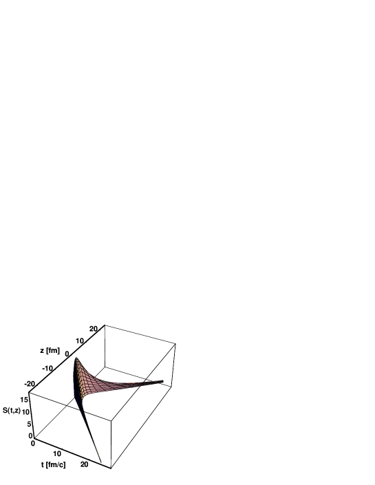
Fig. 13.: The reconstructed $S(t,z)$ emission function in arbitrary units, as a function of time $t$ and longitudinal coordinate $z$. The best fit parameters of $\Delta\eta=1.36$, $y_{0}=0.082$, $\Delta\tau=1.3$ fm/c and ${\overline{\tau}}=1.4$ fm/c are used to obtain this plot. Note that before we made this reconstruction together with the NA22 Collaboration, only 1 fm² area from this extended bumerang shape was visible to the intensity interferometry microscope.

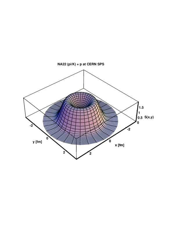
Fig. 14.: The reconstructed $S(r_{x},r_{y})$ emission function in arbitrary vertical units, as a function of the transverse coordinates $r_{x}$ and $r_{y}$. The shape has been reconstructed assuming the validity of a non-relativistic solution of hydrodynamics in the transverse direction, and using the values of $T_{0}$, $\langle\Delta T/T\rangle$ and $\langle u_{t}\rangle$ as obtained from the fits to the single-particle spectra. The root mean square width of the source distribution was obtained from the fits to the NA22 Bose–Einstein correlation functions. The momentum variables and the longitudinal and temporal variables are integrated over.

A reconstruction of the space-time distribution of pion emission points is shown in Fig. 13, expressed as a function of the cms time variable $t$ and the cms longitudinal coordinate $z\equiv r_{z}$. The momentum-integrated emission function along the $z$ axis, i.e. at ${{\mbox{\bf r}}}_{t}=(r_{x},r_{y})=(0,0)$ is given by

$$S(t,z)\propto\exp\left(-{(\tau-{\overline{\tau}})^{2}\over 2\Delta\tau^{2}}\right)\exp\left(-{(\eta-y_{0})^{2}\over 2\Delta\eta^{2}}\right).$$ (162)

It relates the parameters fitted to the NA22 single-particle spectrum and HBT radii to the particle production in space-time. The coordinates $(t,z)$ are expressed with the help of the longitudinal proper-time $\tau$ and space-time rapidity as $\eta$ as $(\tau\cosh(\eta),\tau\sinh(\eta))$.

We find a structure looking like a boomerang, i.e. particle production takes place close to the regions of $z=t$ and $z=-t$, with gradually decreasing probability for ever larger values of space-time rapidity. Although the mean proper-time for particle production is ${\overline{\tau}}=1.4$ fm/c, and the dispersion of particle production in space-time rapidity is rather small, $\Delta\eta=1.35$ fm, we still see a characteristic long tail of particle emission on both sides of the light-cone, giving a total of 40 fm maximal longitudinal extension in $z$ and a maximum of about 20 fm/c duration of particle production in the time variable $t$.

In the transverse direction, only the rms width of the source can be directly inferred from the BP radii. However, the additional information from the analysis of the transverse momentum distribution on the values of $\langle u\rangle_{t}$ and on the values of $\langle\Delta T/T\rangle_{r}$ can be used to reconstruct the details of the transverse density profile, as an exact, non-relativistic hydro solution was found in Ref. [39], given in terms of the parameters $\langle u\rangle_{t}$ and $\langle\Delta T/T\rangle_{r}$ and using an ideal gas equation of state. Assuming the validity of this non-relativistic solution in the transverse direction, in the mid-rapidity range, one can reconstruct the detailed shape of the transverse densityprofile. The result looks like a ring of fire in the $(r_{x},r_{y})$ plane, see Fig. 14. In this hydro solution, $\langle\Delta T/T\rangle_{r}<m\langle u\rangle_{t}^{2}/T_{0}$ corresponds to self-similar, expanding fireballs, while $\langle\Delta T/T\rangle_{r}>m\langle u\rangle_{t}^{2}/T_{0}$ corresponds to self-similar, expanding shells or rings of fire.

Due to the strong surface cooling and the small amount of the transverse flow, one finds that the particle emission in the transverse plane of h + p reactions at CERN SPS corresponds to a ring of fire. This transverse distribution, together with the scaling longitudinal expansion, creates an elongated, tube-like source in three dimensions, with the density of particle production being maximal on the surface of the tube.

12 Pb + Pb Correlations and Spectra at CERN SPS

In Ref. [30], an analysis similar to that of the NA22 Collaboration has been performed, with improved analytic approximations, using Fermi–Dirac or Bose–Einstein statistics $(s=\pm 1)$ in the analytic expressions fitted to single particle spectra. The spectra were evaluated with the binary source method, the Bose–Einstein correlation functions were calculated with the saddle-point method without invoking the binary source picture. The analytical formulas for the BECF and IMD, as were used in the fits, were summarized in their presently most advanced form in Section 8, their development was described in Refs [18, 19, 20, 27, 29, 50].

Fig. 15.: Result of simultaneous fits of the Buda–Lund hydro model to particle correlations and spectra in 158 AGeV Pb + Pb reactions at CERN SPS (data from the NA49 Collaboration)

Fig. 16.: Result of simultaneous fits of the Buda–Lund hydro model to particle correlations and spectra in 158 AGeV Pb + Pb reactions at CERN SPS (data from the NA44 Collaboration)

In case of homogeneous freeze-out temperatures, or particles with small masses, Eq. (156) implies a linear rise of the slope with $m$ [18] as

$$T_{*}(m)=T_{0}+m\langle u\rangle_{t}^{2},\qquad\mbox{\rm if }\quad\Big{\langle}{\Delta T\over T}\Big{\rangle}_{r}\ll T_{0}/m.$$ (163)

For heavy particles, or for large, non-vanishing temperature gradients, a flattening of the initial linear rise is obtained [18] as

$$T_{*}(m)=T_{0}\left[1+\frac{\langle u\rangle_{t}^{2}}{\big{\langle}{\Delta T\over T}\big{\rangle}_{r}}\right],\qquad\mbox{\rm if }\quad\Big{\langle}{\Delta T\over T}\Big{\rangle}_{r}\gg T_{0}/m.$$ (164)

This means that very heavy particles resolve the temperature inhomogeneities of the source, and they are produced with a mass-independent effective slope parameter in the BL-H parameterization, if $T_{0}/m$ becomes smaller than the temperature inhomogeneity. In a general case, the $T_{*}(m)$ function starts with an initial linear $m$ dependence, with a slope given by the transverse flow $\langle u\rangle_{t}$, then $T_{*}(m)$ flattenes out to a mass-independent value if the source has temperature inhomogeneities in the transverse direction. Such a behavior was reported by Pb + Pb heavy ion experiments at CERN SPS [5]. The central temperature is [30] $T_{0}\approx 140$ MeV, the flattening of the slopes sets in at about $m=1400$ MeV [9], which then leads to about 10% temperature inhomogeneity in the transverse direction of the Pb + Pb source. This estimate is in a good agreement with the results of the combined analysis of the single-particle spectra and the two-particle Bose–Einstein correlation functions, see Table 5.

Table 5.: Fit paramaters of Buda–Lund hydro (BL-H) in a simultaneous analysis of NA49, NA44 and preliminary WA98 spectra and correlation data

Parameter	NA49	NA44	WA98	Averaged
$T_{0}$ [MeV]	$134\pm 3\ \ \$	$145\pm 3\ \ \$	$139\pm 5\ \ \$	$139\pm 6\ \ \$
$\langle u_{t}\rangle$	$0.61\pm 0.05$	$0.57\pm 0.12$	$0.50\pm 0.09$	$0.55\pm 0.06$
$R_{G}$ [fm]	$7.3\pm 0.3$	$6.9\pm 1.1$	$6.9\pm 0.4$	$7.1\pm 0.2$
$\tau_{0}$ [fm/c]	$6.1\pm 0.2$	$6.1\pm 0.9$	$5.2\pm 0.3$	$5.9\pm 0.6$
$\Delta\tau$ [fm/c]	$2.8\pm 0.4$	$0.01\pm 2.2$	$2.0\pm 1.9$	$1.6\pm 1.5$
$\Delta\eta$	$2.1\pm 0.2$	$2.4\pm 1.6$	$1.7\pm 0.1$	$2.1\pm 0.4$
$\langle{\Delta T/T}\rangle_{r}$	$0.07\pm 0.02$	$0.08\pm 0.08$	$0.01\pm 0.02$	$0.06\pm 0.05$
$\langle{\Delta T/T}\rangle_{t}$	$0.16\pm 0.05$	$0.87\pm 0.72$	$0.74\pm 0.08$	$0.59\pm 0.38$
$\chi^{2}$/NDF	163/98 = 1.66	63/71 = 0.89	115/108 = 1.06	1.20

The NA49, NA44 and WA98 data on single particle spectra of h^-, identified $\pi$, K and p as well as detailed rapidity and $m_{t}$ dependent HBT radius parameters are found to be consistent with each other as well as with BL-H. The BL-H fit results to these data sets is summarized in Table 5, Ref. [30].

13 Comparison of h + p and Pb + Pb Final States at CERN SPS with Heavy Ion Reactions at Low and Intermediate Energies

The final state of central Pb + Pb collisions at CERN SPS corresponds to a cylindrically symmetric, large ($R_{G}=7.1\pm 0.2$ fm) and transversally homogenous ($T_{0}=139\pm 6$ MeV) fireball, expanding three-dimensionally with $\langle u_{t}\rangle=0.55\pm 0.06$. A large mean freeze-out time, ${\overline{\tau}}=5.9\pm 0.6$ is found with a relatively short duration of emission, $\Delta{\overline{\tau}}=1.6\pm 1.5$ fm, which is similar to the time-scale of emission in the h + p reaction. Note that the temporal cooling in Pb + Pb reactions seems to be stronger than in h + p, which can be expained by the faster, three-dimensional expansion in the former case, as compared to the essentially one-dimensional expansion in the case of h + p reactions. By the time the particle production is over, the surface of Pb + Pb collisions cools down from 139 MeV to $T_{0}/(1+\langle\Delta T/T_{0}\rangle_{r})/(1+\langle\Delta T/T_{0}\rangle_{t})\approx 83$ MeV. It is very interesting to note that this value is similar to the surface temperature of $T_{s}=82\pm 7$ MeV, found in h + p reactions as a consequence of the transverse temperature inhomogeneities, as described in Section 11, Ref. [50]. Such snowballs with relatively low values of surface temperature $T_{s}$ and a possible hotter core were reported first in 200 AGeV S + Pb reactions in Ref. [19].

Other hydro parameterizations, as reviewed in Ref. [9], frequently neglect the effects of temperature inhomogeneities during the expansion and particle production stage. Energy conservation implies that the temperature cannot be exactly constant when particles are freezing out in a non-vanishing period of time from a three-dimensionally expanding source.

The exact solution of non-relativistic, spherically symmetric fireball hydrodynamics implies [38, 18] that Gaussian fireballs with spatially uniform temperature profiles satisfy the collisionless Boltzmann equation.

Fixing the temperature to a constant in the fits yields an average freeze-out temperature in the range of $T_{f}=110\pm 30$ MeV [9, 19, 25, 24].

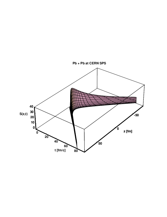
Fig. 17.: The reconstructed $S(t,z)$ emission function in arbitrary units, as a function of time $t$ and longitudinal coordinate $z$, for 158 AGeV Pb + Pb reactions

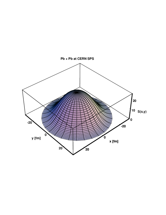
Fig. 18.: The reconstructed $S(r_{x},r_{y})$ emission function in arbitrary units, as a function of the transverse coordinates $r_{x}$ and $r_{y}$

Based on the recently found new family of non-relativistic hydrodynamics [39] and on the analysis of h + p single particle spectra and two-particle Bose–Einstein correlation function [50], we concluded that the pion emission function $S(r_{x},r_{y})$ in h + p reactions corresponds to the formation of a ring of fire in the transverse plane, because the transverse flow is rather small and because the sudden drop of the temperature in the transverse direction leads to large pressure gradients in the center and small pressure gradients and a density built-up at the expanding radius of the fire-ring. We presented arguments for a similar formation of a spherical shell of fire in the proton distributions at 30 AMeV ⁴⁰Ar + ¹⁹⁷Au reactions.

The formation of shells of fire seems thus to be of a rather generic nature, related to the initial conditions of self-similar radial flows. It is natural to ask the question: can we learn more about this phenomena in other physical systems?

Radial expansion is a well established phenomena in heavy ion collisions from low energy to high energy reactions. See Refs [117, 118] for recent reviews and for example see Refs [125, 126, 127, 128] for the evidence of collective flow in central heavy ion collisions from 100 AMeV to 2 AGeV as measured by the FOPI Collaboration at GSI SIS.

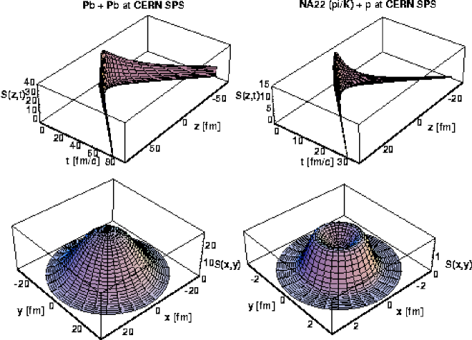
Fig. 19.: Comparison of the reconstructed $S(t,z)$ and $S(r_{x},r_{y})$ emission functions for 250 GeV/c h + p reactions and for for 158 AGeV Pb + Pb reactions at CERN SPS. Note the different characteristic scales in the transverse and the temporal directions, and the different shapes of the transverse density distribution.

The FOPI Collaboration measured recently the proton–proton correlation functions at 1.93 AGeV Ni + Ni collisions [128]. To interpret their data, they utilized a version of the hydrodynamical solution, found in Ref. [38]. They assumed a linear flow profile, a Gaussian density distribution and a constant temperature. Such a solution of fireball hydrodynamics exists, but it corresponds to a collisionless Knudsen gas [38, 39]. A collisionless approximation has to break down. Indeed, only the peak of the FOPI proton–proton correlation function was reproduced by the collisionless model, however, the tails had to be excluded from the FOPI analysis. Perhaps it is worthwhile to search for a possible formation of shells of fire at the SIS energy domain, by re-analyzing the FOPI data [39].

14 Shells of Fire and Planetary Nebulae

In transport calculations based on the Boltzmann–Uehling–Uhlenbeck equation, a formation of toroidal density distributions was predicted for central ³⁶Ar + ⁴⁵Sc collisions at $E=80$ AMeV in Ref. [120], which leads to ring-like configurations for $S(r_{x},r_{y})$.

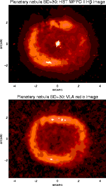
Fig. 20.: Planetary nebula BD+30 imaged by the Hubble Space Telescope (top) and by the Very Large Array (VLA) radiotelescope in New Mexico (bottom). The latter indicates a complete ring of fire, dust blocks some of the visible light on the upper image.

However, the clearest experimental observation of the development of expanding shell like structures in the time evolution of exploding fireballs comes from stellar astronomy. Stars with initial masses of less than about eight solar masses end their lives by ejecting planetary nebulae, stellar remnants turning to white dwarfs. After the star has completed its core hydrogen burning, it becomes a red giant. In the core of the star, helium burns while hydrogen continues to burn in a thin shell surrounding the core. This hydrogen rich shell swells to enormous size, and the surface temperature drops to a rather low value for stars. A solar wind develops that carries away most of the hydrogen envelope surrounding the star’s central core. The envelope material ejected by the star forms an expanding shell of gas that is known as a planetary nebula. Planetary nebulae are illuminated by their central stars and display a variety of often beautiful structures. Some are spherical or helical, others have bipolar shapes, and still others are rather irregularly shaped. In a matter of a few tens of thousands of years, they intermingle with the interstellar medium and disperse.

The space-time evolution of planetary nebulae is in many aspects similar to the solution of non-relativistic hydrodynamics given in Ref. [39]. We argued, that this solution seems to describe also low and intermediate heavy ion collisions in the 30 – 80 AMeV energy domain. A similar hydro solution may also describe the non-relativistic transverse dynamics at mid-rapidity in hadron + proton collisions in the CERN SPS energy domain, compare Figs  14 and 20, the latter from Ref. [129].

In all of these physical systems, expansion competes with the drop of the pressure gradients, which in turn is induced by the drop of the temperature on the surface. If the flow is small enough, the drop of the temperature on the surface results in a drop of the pressure gradients on the surface, which implies density pile-up. On the other hand, if the flow is strong enough, it blows away the material from the surface, preventing the formation of shells of fire, and an ordinary expanding fireball is obtained.

Finally I note that this situation is just a special class of the more general solutions given in Ref. [39]. Arbitrary number of self-similarly expanding, simultaneously existing shells of fire can be described by the general form of new class of exact solutions of fireball hydrodynamics [39].

15 Signal of Partial $U_{A}(1)$ Symmetry Restoration from Two-Pion Bose–Einstein Correlations

In this section let me summarize Ref. [74], where the effective intercept parameter of the two-pion Bose–Einstein Correlation function, $\lambda_{*}$ was shown to carry a sensitive and measurable signal of partial restoration of the axial $U_{A}(1)$ symmetry and the related increase of the $\eta^{\prime}$ production in ultra-relativistic nuclear collisions: An increase in the yield of the $\eta^{\prime}$ meson, proposed earlier as a signal of partial $U_{A}(1)$ restoration, was shown to create a “hole” in the low $p_{t}$ region of $\lambda_{*}$.

Fig. 21.: Using the estimates of pion abundances given by Fritiof, the solid line represents $\lambda_{*}(m_{t})$ assuming normal $\eta^{\prime}$ abundances while the other lines represent $\lambda_{*}(m_{t})$ with a factor of 3 (dashed), 16 (dotted) and 50 (dot–dashed) enhancement of $\eta^{\prime}$ due to partial $U_{A}(1)$ chiral symmetry restoration and the corresponding decrease of the $\eta^{\prime}$ mass in the hot and dense region. All curves are calculated for $T_{0}=140$ MeV and $\langle u_{t}\rangle=0.5$. The datapoints are from 200 AGeV central S + Pb reactions at CERN SPS, as measured by the NA44 Collaboration.

In the chiral limit ($m_{u}=m_{d}=m_{s}=0$), QCD possesses a $U(3)$ chiral symmetry. When broken spontaneously, $U(3)$ implies the existence of nine massless Goldstone bosons. In Nature, there are only eight light pseudoscalar mesons, a discrepancy which is resolved by the Adler–Bell–Jackiw $U_{A}(1)$ anomaly; the ninth would-be Goldstone boson gets a mass as a consequence of the non-zero density of topological charges in the QCD vacuum [141, 140]. In Refs [132, 133], it is argued that the ninth (“prodigal” [132]) Goldstone boson, the $\eta^{\prime}$, would be abundantly produced if sufficiently hot and dense hadronic matter is formed in nucleus–nucleus collisions. Estimates of Ref. [132] show that the corresponding production cross section of the $\eta^{\prime}$ should be enhanced by a factor of 3 up to 50 relative to that for p + p collisions.

If the $\eta^{\prime}$ mass is decreased, a large fraction of the $\eta^{\prime}$s will not be able to leave the hot and dense region through thermal fluctuation since they need to compensate for the missing mass by large momentum [132, 133, 134]. These $\eta^{\prime}$s will thus be trapped in the hot and dense region until it disappears, after which their mass becomes normal again; as a consequence, the $\eta^{\prime}$-s will have small transverse momenta $p_{t}$. Then they decay to pions via

$$\eta^{\prime}\rightarrow\eta+\pi^{+}+\pi^{-}\rightarrow(\pi^{0}+\pi^{+}+\pi^{-})+\pi^{+}+\pi^{-}.$$ (165)

It is important to observe that the $p_{t}$ of pions produced in this decay chain is small since many of the $\eta^{\prime}$ appear at $p_{t}\simeq 0$ and also since the rest mass of the decay products from the $\eta^{\prime},\eta$ decays use up most of the remaining energy. Based on the kinematics of the $\eta^{\prime},\eta$ decay chain to pions, an enhanced production of $\pi$ mesons was estimated to happen dominantly in the $p_{t}\simeq 150$ MeV region, extending to a maximum $p_{t}\simeq 407$ MeV [67]. In the core/halo picture the $\eta^{\prime},\eta$ decays contribute to the halo due to their large decay time ($1/{\Gamma_{\eta^{\prime},\eta}}\gg 20$ fm/c). Thus, we expect a hole in the $0\leq p_{t}\leq 150$ MeV region of the effective intercept parameter, $\lambda_{*}=[N_{\rm core}({\bf p})/N_{\rm total}({\bf p})]^{2}$.

To calculate the $\pi^{+}$ contribution from the halo region, the bosons ($\omega$, $\eta^{\prime}$, $\eta$ and ${\mathrm{K}}^{0}_{S}$) are given both a rapidity $(-1.0<y<1.0)$ and an $m_{t}$, then are decayed using Jetset 7.4 [137]. The $m_{t}$ distribution [18, 76] of the bosons is given by

$$N(m_{t})=Cm_{t}^{\alpha}e^{-m_{t}/T_{\rm eff}},$$ (166)

where $C$ is a normalization constant, $\alpha=1-d/2$ and where [18, 14]

$$T_{\rm eff}=T_{\rm fo}+m\langle u_{t}\rangle^{2}.$$ (167)

In the above expression, $d=3$ is the dimension of expansion, $T_{\rm fo}=140$ MeV is the freeze-out temperature and $\langle u_{t}\rangle$ is the average transverse flow velocity. It should be noted that the $m_{t}$ distribution for the core pions is also obtained from Eq. (166). The contributions from the decay products of the different regions (halo and core) are then added together according to their respective fractions, allowing for the determination of $\lambda_{*}(m_{t})$. The respective fractions of pions are estimated separately by Fritiof [135] and by RQMD [139] as summarized in Ref. [136].

Fig. 22.: Using the estimates of pion abundances given by Fritiof, $\lambda_{*}(m_{t})$ is calculated using $\langle u_{t}\rangle=0.00$ (solid line), $\langle u_{t}\rangle=0.25$ (dashed line), $\langle u_{t}\rangle=0.50$ (dotted line) and $\langle u_{t}\rangle=0.75$ (dashed–dotted line)

Simulating the presence of the hot and dense region involves increasing the relative abundance of the $\eta^{\prime}$ and also changing their $p_{t}$ spectrum. The $p_{t}$ spectrum of the $\eta^{\prime}$ is obtained by assuming energy conservation and zero longitudinal motion at the boundary between the two phases. This conservation of transverse mass at the boundary implies

$$m^{*2}_{\eta^{\prime}}+{p_{t}}^{*2}_{\eta^{\prime}}=m^{2}_{\eta^{\prime}}+{p_{t}}^{2}_{\eta^{\prime}},$$ (168)

where the $*$ denotes the $\eta^{\prime}$ in the hot dense region. The $p_{t}$ distribution then becomes a two-fold distribution. The first part of the distribution is from the $\eta^{\prime}$ which have $p_{t}^{*}\leq[m^{2}_{\eta^{\prime}}-m^{*2}_{\eta^{\prime}}]^{1/2}$. These particles are given a $p_{t}=0$. The second part of the distribution comes from the rest of the $\eta^{\prime}$’s which have big enough $p_{t}$ to leave the hot and dense region. These have the same, flow motivated $p_{t}$ distribution as the other produced resonances and are given a $p_{t}$ according to the $m_{t}$ distribution

$$N_{\eta^{\prime}}(m^{*}_{t})=C{m^{*}_{t}}^{-0.5}e^{-m^{*}_{t}/T^{\prime}},$$ (169)

where $C$ is a normalization constant and where $T^{\prime}=200$ MeV and $m^{*}_{\eta^{\prime}}$ is the effective temperature and mass, respectively, of the hot and dense region. Using the value given above for the effective temperature and letting $m^{*}_{\eta^{\prime}}=500$ MeV implies an increase in the production cross section of the $\eta^{\prime}$ in the hot and dense region by a factor of 10.

Using three different effective masses for the $\eta^{\prime}$ in the hot and dense region, calculations of $\lambda_{*}(m_{t})$ including the hot and dense regions are compared to those assuming the standard abundances in Fig. 21. A similar $m_{t}$ dependence but with slightly higher values of $\lambda_{*}(m_{t})$ is obtained when using RQMD abundances. The effective mass of 738 MeV corresponds to an enhancement of the production cross section of the $\eta^{\prime}$ by a factor of 3, while the effective mass of 403 MeV and 140 MeV correspond to factors of 16 and 50 respectively. The two data points shown are taken from NA44 data on central S + Pb reactions at the CERN SPS with incident beam energy of 200 AGeV [15]. The lowering of the $\eta^{\prime}$ mass and the partial chiral restoration result in a hole in the effective intercept parameter at low $m_{t}$. This happens even for a modest enhancement of a factor of 3 in the $\eta^{\prime}$ production. Similar results are obtained when using RQMD abundances. See Ref. [67] for further details of the simulation.

In addition, $\lambda_{*}(m_{t})$ is calculated using Fritiof abundances with different average flow velocities in Fig. 22. Here it is shown that $\lambda_{*}(m_{t})$ can also be a measure of the average collective flow. In Ref. [67], an average flow velocity of $\langle u_{t}\rangle=0.50$ resulted in an approximately flat, $m_{t}$ independent shape for the effective intercept parameter $\lambda_{*}(m_{t})$ distribution [67]. Calculations using RQMD abudances result in a similar dependence on $\langle u_{t}\rangle$, but with slightly higher values of $\lambda_{*}(m_{t})$.

This analysis of NA44 S + Pb data indicated no visible sign of $U_{A}(1)$ restoration at SPS energies. In addition, a mean transverse flow of $\langle u_{t}\rangle\approx 0.50$ in S + Pb reactions was deduced [67]. The suggested $\lambda_{*}$-hole signal of partial $U_{A}(1)$ restoration cannot be faked in a conventional thermalized hadron gas scenario, as it is not possible to create significant fraction of the $\eta$ and $\eta^{\prime}$ mesons with $p_{t}\simeq 0$ in such a case, Ref. [67].

16 Squeezed Correlations and Spectra for Mass-Shifted Bosons

In this section, let me follow the lines of Refs [69, 70] to show that novel back-to-back correlations (BBC) arise for thermal ensembles of squeezed bosonic states associated with medium-modified mass shifts. It was observed in Ref. [70], that the strength of the BBC could become unexpectedly large in heavy ion collisions, and may thus provide an experimentally observable signal of boson modification in hot and dense matter.

Consider, in the rest frame of matter, the following model Hamiltonian,

$${H}=H_{0}-\frac{1}{2}\int d^{3}{\bf x}d^{3}{\bf y}\phi({\bf x})\delta M^{2}({\bf x}-{\bf y})\phi({\bf y}),$$ (170)

where $H_{0}$ is the asymptotic Hamiltonian,

$$H_{0}=\frac{1}{2}\int d^{3}{\bf x}\left(\dot{\phi}^{2}+|\nabla\phi|^{2}+m_{0}^{2}\phi^{2}\right).$$ (171)

The scalar field $\phi({\bf x})$ in this Hamiltonian, $H$, corresponds to quasi-particles that propagate with a momentum-dependent medium-modified effective mass, which is related to the vacuum mass, $m_{0}$, via

$$m_{*}^{2}({|{\bf k}|})=m_{0}^{2}-\delta M^{2}({|{\bf k}|}).$$

The mass shift is assumed to be limited to long wavelength collective modes:

$$\delta M^{2}({|{\bf k}|})\ll m_{0}^{2}\quad\quad\mbox{\rm if}\quad|{\bf k}|>\Lambda_{s}.$$

The invariant single-particle and two-particle momentum distributions are given as:

$$N_{1}({\bf k}_{1}) = \omega_{{\bf k}_{1}}{d^{3}N\over d{\bf k}_{1}}=\omega_{{\bf k}_{1}}\langle a^{\dagger}_{{\bf k}_{1}}a^{\phantom{\dagger}}_{{\bf k}_{1}}\rangle,$$ (172)

$$N_{2}({\bf k}_{1},{\bf k}_{2}) = \omega_{{\bf k}_{1}}\omega_{{\bf k}_{2}}\langle a^{\dagger}_{{\bf k}_{1}}a^{\dagger}_{{\bf k}_{2}}a^{\phantom{\dagger}}_{{\bf k}_{2}}a^{\phantom{\dagger}}_{{\bf k}_{1}}\rangle,$$ (173)

$$\langle a^{\dagger}_{{\bf k}_{1}}a^{\dagger}_{{\bf k}_{2}}a^{\phantom{\dagger}}_{{\bf k}_{2}}a^{\phantom{\dagger}}_{{\bf k}_{1}}\rangle = \langle a^{\dagger}_{{\bf k}_{1}}a^{\phantom{\dagger}}_{{\bf k}_{1}}\rangle\langle a^{\dagger}_{{\bf k}_{2}}a^{\phantom{\dagger}}_{{\bf k}_{2}}\rangle+\langle a^{\dagger}_{{\bf k}_{1}}a^{\phantom{\dagger}}_{{\bf k}_{2}}\rangle\langle a^{\dagger}_{{\bf k}_{2}}a^{\phantom{\dagger}}_{{\bf k}_{1}}\rangle$$ (174)

$$+\langle a^{\dagger}_{{\bf k}_{1}}a^{\dagger}_{{\bf k}_{2}}\rangle\langle a^{\phantom{\dagger}}_{{\bf k}_{2}}a^{\phantom{\dagger}}_{{\bf k}_{1}}\rangle,$$

where $a_{\bf k}$ is the annihilation operator for asymptotic quanta with four-momentum $k^{\mu}\,=\,(\omega_{\bf k},{\bf k})$, $\omega_{\bf k}=\sqrt{m^{2}+{\bf k}^{2}}$ and the expectation value of an operator $\hat{O}$ is given by the density matrix $\hat{\rho}$ as $\langle\hat{O}\rangle={\rm Tr}\,\hat{\rho}\,\hat{O}$. Eq.(174) has been derived as a generalization of Wick’s theorem for locally equilibriated (chaotic) systems in Ref. [105].

The chaotic and squeezed amplitudes were introduced [70] as

$$G_{c}(1,2) = \sqrt{\omega_{{\bf k}_{1}}\omega_{{\bf k}_{2}}}\langle a^{\dagger}_{{\bf k}_{1}}a^{\phantom{\dagger}}_{{\bf k}_{2}}\rangle,$$ (175)

$$G_{s}(1,2) = \sqrt{\omega_{{\bf k}_{1}}\omega_{{\bf k}_{2}}}\langle a^{\phantom{\dagger}}_{{\bf k}_{1}}a^{\phantom{\dagger}}_{{\bf k}_{2}}\rangle.$$ (176)

In most situations, the chaotic amplitude, $G_{c}(1,2)\equiv G(1,2)$ is dominant, and carries the Bose–Einstein correlations, while the squeezed amplitude, $G_{s}(1,2)$ vanishes.

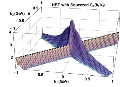
Fig. 23.: Illustration of the new back-to-back correlations for mass-shifted $\pi^{0}$ pairs, assuming $T=140$ MeV, $G_{c/s}(p_{1},p_{2})\propto\exp[-q_{12}^{2}R_{G}^{2}/2]$, with $R_{G}=2$ fm. The fall of BBC for increasing values of $|{\bf k}|$ is controlled here by a momentum-dependent effective mass, $m_{\pi,*}=m_{\pi}[1+\exp(-{\bf k}^{2}/\Lambda_{s}^{2})]$, with $\Lambda_{s}=325$ MeV in the sudden approximation.

16.1 Mass modification in a homogenous heat bath

The terms involving $G_{s}(1,2)$ become non-negligible when mass shift becomes non-vanishing, i.e. $\delta M^{2}({\bf k})\neq 0$. Given such a mass shift, the dispersion relation is modified to $\Omega_{\bf k}^{2}=\omega^{2}_{\bf k}-\delta M^{2}({\bf k})$, where $\Omega_{\bf k}$ is the frequency of the in-medium mode with momentum ${\bf k}$. The annihilation operator for the in-medium quasi-particle $b_{\bf k}$, and that of the asymptotic field, $a_{\bf k}$, are related by a Bogolyubov transformation [69]:

$$a^{\phantom{\dagger}}_{{\bf k}_{1}}=c^{\phantom{\dagger}}_{{\bf k}_{1}}b^{\phantom{\dagger}}_{{\bf k}_{1}}+s^{*\phantom{\dagger}}_{-{\bf k}_{1}}b^{\dagger}_{-{\bf k}_{1}}\equiv C^{\phantom{\dagger}}_{1}+S^{\dagger}_{-1},$$ (177)

where $c_{\bf k}=\cosh[r_{\bf k}]$, $s_{\bf k}=\sinh[r_{\bf k}]$ and $r_{\bf k}$ reads as

$$r_{\bf k}=\frac{1}{2}\log(\omega_{\bf k}/\Omega_{\bf k})\;\;.$$ (178)

We introduce the shorthand, $C^{\phantom{\dagger}}_{1}$ and $S_{-1}^{\dagger}$, to simplify later notation. As the Bogolyubov is a squeezing transformation, let us call $r_{\bf k}$ mode dependent squeeze parameter. While it is the $a$-quanta that are observed, it is the $b$-quanta that are thermalized in medium [153]. Let us consider the average for a globally thermalized gas of the $b$-quanta, that is homogenous in volume $V$:

$$\hat{\rho}={\displaystyle\phantom{|}1\over Z}\exp\left(-\frac{1}{T}\frac{V}{(2\pi)^{3}}\int d^{3}{\bf k}\,\Omega_{\bf k}\,b^{\dagger}_{\bf k}b^{\phantom{\dagger}}_{\bf k}\right).$$ (179)

When this thermal average is applied,

$$G_{c}(1,2) = \sqrt{\omega_{{\bf k}_{1}}\omega_{{\bf k}_{2}}}\left[\langle C^{\dagger}_{1}C^{\phantom{\dagger}}_{2}\rangle+\langle S^{\phantom{\dagger}}_{-1}S^{\dagger}_{-2}\rangle\right],$$ (180)

$$G_{s}(1,2) = \sqrt{\omega_{{\bf k}_{1}}\omega_{{\bf k}_{2}}}\left[\langle S^{\dagger}_{-1}C^{\phantom{\dagger}}_{2}\rangle+\langle C^{\phantom{\dagger}}_{1}S^{\dagger}_{-2}\rangle\right].$$ (181)

If this thermal $b$ gas freezes out suddenly at some time at temperature $T$, the observed single $a$-particle distribution takes the following form:

$$N_{1}({\bf k}) = \frac{V}{(2\pi)^{3}}\,\omega_{\bf k}\,n_{1}({\bf k}),$$ (182)

$$n_{1}({\bf k}) = |c_{\bf k}^{\phantom{\dagger}}|^{2}n_{\bf k}^{\phantom{\dagger}}+|s_{-\bf k}|^{2}(n_{-\bf k}+1),$$ (183)

$$n_{\bf k} = \frac{1}{\exp(\Omega_{\bf k}/T)-1}\;.$$ (184)

This spectrum includes a squeezed vacuum contribution in addition to the mass-modified thermal spectrum.

In this homogeneous limiting case, the two particle correlation function is unity except for the parallel (HBT) and antiparallel (BBC) cases:

$$C_{2}({\bf k},{\bf k}) = 2,$$ (185)

$$C_{2}({\bf k},{\bf-k}) = 1+{\displaystyle\phantom{|}{|c^{*}_{\bf k}s_{\bf k}^{\phantom{\dagger}}n_{\bf k}^{\phantom{\dagger}}+c^{*}_{-\bf k}s_{-\bf k}^{\phantom{\dagger}}(n_{-\bf k}^{\phantom{\dagger}}+1)|^{2}}\over\displaystyle\phantom{|}{n_{1}({\bf k})\,n_{1}({-\bf k})}}.$$ (186)

The dynamical correlation due to the two mode squeezing associated with mass shifts is therefore back-to-back, as first pointed out in Ref. [69]. The strength of the HBT correlations remains 2 for identical momenta.

It follows from Eq. (186) that the intercept of the BBC is unlimited from above: $1\leq C_{2}({\bf k},-{\bf k})<\infty$. As $|{\bf k}|\rightarrow\infty$, $C_{2}({\bf k},-{\bf k})\simeq 1+1/|s_{-{\bf k}}|^{2}\simeq 1+1/n_{1}({\bf k})\rightarrow\infty$. Hence, at large values of $|{\bf k}|$, the particle production is dominated by that of back-to-back correlated pairs for any non-vanishing value of the in-medium mass shifts [70].

16.2 Suppression by finite duration of emission

To describe a more gradual freeze-out, the probability distribution $F(t_{i})$ of the decay times $t_{i}$ is introduced. The sudden approximation is recovered in the $F(t_{i})=\delta(t_{i}-t_{0})$ limiting case. The time evolution of the operators is given by $a_{\bf k}(t)=a_{\bf k}(t_{i})\exp[-i\omega_{\bf k}(t-t_{i})]$. This leads to a suppression of BBC as

$$C_{2}({\bf k},-{\bf k})=1+|\tilde{F}(\omega_{\bf k}+\omega_{-{\bf k}})|^{2}{\displaystyle\phantom{|}{|c^{*}_{\bf k}s_{\bf k}^{\phantom{\dagger}}n_{\bf k}^{\phantom{\dagger}}+c^{*}_{-\bf k}s_{-\bf k}^{\phantom{\dagger}}(n_{-\bf k}^{\phantom{\dagger}}+1)|^{2}}\over\displaystyle\phantom{|}{n_{1}({\bf k})\,n_{1}({-\bf k})}}.$$ (187)

Here $\tilde{F}(\omega)=\int dtF(t)\exp(-i\omega t)$, so for an exponential decay, $F(t)=\Theta(t-t_{0})\times$ $\Gamma\exp[-\Gamma(t-t_{0})]$ the suppression factor is

$$|\tilde{F}(\omega_{\bf k}+\omega_{-{\bf k}})|^{2}=1/[1+(\omega_{\bf k}+\omega_{-{\bf k}})^{2}/\Gamma^{2}].$$ (188)

In the adiabatic limit, $\Gamma\rightarrow 0$, this factor suppresses completely the BBC, while in the sudden approximation, $\Gamma\rightarrow\infty$, the full strenght of the BBC is preserved. For a typical $\delta t=\hbar/\Gamma=2$ fm/c decay time, and for BBC of $\phi$ mesons with $m_{*}=0.6-1.4$ GeV, this suppression factor is about 0.001, which decreases the BBC of $\phi$ mesons from the scale of 2000 to 2, the scale of the HBT correlations. This emphasizes the enormous strength of the BBC [70].

The formalism to evaluate the BBC for locally thermalized, expanding sources was also developed, see Ref. [70] for greater details.

As the Bogolyubov transformation always mixes particles with anti-particles, the above considerations hold only for particles that are their own anti-particles, e.g. the $\phi$ meson and $\pi^{0}$. The extension to particle–anti-particle correlations is straightforward. Let $+$ label particles, $-$ antiparticles if antiparticle is different from particle, let $0$ label both particle and antiparticle if they are identical. The non-trivial correlations from mass modification for pairs of $(++)$, $(+-)$ and $(00)$ type read as follows:

$$C^{++}_{2}({\bf k}_{1},{\bf k}_{2})\! = \!1+{|G_{c}(1,2)|^{2}\over G_{c}(1,1)G_{c}(2,2)},$$ (189)

$$C^{+-}_{2}({\bf k}_{1},{\bf k}_{2})\! = \!1+{|G_{s}(1,2)|^{2}\over G_{c}(1,1)G_{c}(2,2)},$$ (190)

$$C^{00}_{2}({\bf k}_{1},{\bf k}_{2})\! = \!1+{|G_{c}(1,2)|^{2}\over G_{c}(1,1)G_{c}(2,2)}+{|G_{s}(1,2)|^{2}\over G_{c}(1,1)G_{c}(2,2)},$$ (191)

where we assume that mass modifications of particles and anti-particles are the same as happens at vanishing baryon density.

This theory of particle correlations and spectra for bosons with in-medium mass shifts predicts huge back-to-back correlations of $\phi^{0},\phi^{0}$ and ${\mathrm{K}}^{+},{\mathrm{K}}^{-}$ meson pairs [70]. These BBC could become observable at the STAR and PHENIX heavy ion experiments at RHIC [145], and could be looked for in present CERN SPS experiments. Further model calculations are required to study the mass-shift effects on realistic source models.

17 A Pion-Laser Model and Its Solution

In high energy heavy ion collisions hundreds of bosons are created in the present CERN SPS reactions when Pb + Pb reactions are measured at 160 AGeV laboratory bombarding energy. At the RHIC accelerator, thousands of pions could be produced in a unit rapidity interval [5]. If the number of pions in a unit value of phase-space is large enough these bosons may condense into the same quantum state and a pion laser could be created [53].

In this section a consequent quantum mechanical description of multi-boson systems is reviewed, based on properly normalized projector operators for overlapping multi-particle wave-packet states and a model of stimulated emission, following the lines of Refs [55, 56, 61]. One of the new analytic results is that multi-boson correlations generate momentum-dependent radius and intercept parameters even for static sources, as well as induce a special directional dependence of the correlation function. This is to be contrasted to the simplistic but very frequently invoked picture of Eq. (3), where sources without expansion correspond to a correlation function that depends only on the relative momentum, but not on the mean momentum of the particle pairs.

A solvable density matrix of a generic quantum mechanical system is

$$\hat{\rho}\! = \!\sum_{n=0}^{\infty}\,{\displaystyle\phantom{|}{p}_{n}\over\displaystyle\phantom{|}{\cal N}{(n)}}\!\int\!\!\,\,\prod_{i=1}^{n}d\alpha_{i}\rho_{1}(\alpha_{i})\!\left(\sum_{\sigma^{(n)}}\prod_{k=1}^{n}\,\langle\alpha_{k}|\alpha_{\sigma_{k}}\rangle\right)\,|\alpha_{1},...,\alpha_{n}\rangle\langle\alpha_{1},...,\alpha_{n}|\,.$$

Here the index $n$ characterizes sub-systems with particle number fixed to $n$, the multiplicity distribution is prescribed by the set of $\left\{{p}_{n}\right\}_{n=0}^{\infty}$, normalized as $\sum_{n=0}^{\infty}p_{n}=1$. The density matrixes are normalized as $\mbox{Tr}\,\hat{\rho}=1$ and $\mbox{Tr}\,\hat{\rho}_{n}=1$. The states $|\alpha_{1},...,\alpha_{n}\rangle$ denote properly normalized $n$-particle wave-packet boson states:

$$|\ \alpha_{1},\ ...\ ,\ \alpha_{n}\rangle={\left({\displaystyle{\sum_{\sigma^{(n)}}\prod_{i=1}^{n}\langle\alpha_{i}|\alpha_{\sigma_{i}}\rangle}}\right)^{-{1\over 2}}}\!\!\ \alpha^{{\dagger}}_{n}\ ...\ \alpha_{1}^{{\dagger}}|0\rangle.$$ (193)

Here $\sigma^{(n)}$ denotes the set of all the permutations of the indexes $\left\{1,2,...,n\right\}$ and the subscript sized ${\sigma_{i}}$ denotes the index that replaces the index $i$ in a given permutation from $\sigma^{(n)}$. The wave-packet creation operators, $\alpha_{i}^{{\dagger}}$ create the normalized single-particle states $|\alpha_{i}\rangle=\alpha_{i}^{{\dagger}}|0\rangle$, with $\langle\alpha_{i}|\alpha_{i}\rangle=1$. The $\alpha_{i}=(\xi_{i},\pi_{i},\sigma_{i},t_{i})$ stands for a given value of the parameters of a single-particle wave-packet: the mean coordinate, the mean momentum, the width of the wave-packet in coordinate space and the time of the production. The distribution function $\rho_{1}(\alpha_{i})$ provides the probability distribution for a given value of the wave-packet parameters. For simplicity, we assume a static source at rest, uniform wave-packet widths and simultaneous production, $\sigma_{i}=\sigma$ and $t_{i}=t_{0}$. A Gaussian distribution of the centers of wave-packets is also assumed: in the coordinate space, the distribution of $\xi_{i}$ is a characterized with a radius $R$, while in the momentum-space, the centers of wave-packets $\pi_{i}$ are assumed to have a non-relativistic Boltzmann distribution corresponding to a temperature $T$ and mass $m$. The coefficient of proportionality, ${\cal N}{(n)}$, can be determined from the normalization condition.

The density matrix given in Eq. (LABEL:e:dtrick) describes a quantum-mechanical wave-packet system with induced emission, and the amount of the induced emission is controlled by the overlap of the $n$ wave-packets [56], yielding a weight in the range of $[1,n!]$. Although it is very difficult numerically to operate with such a wildly fluctuating weight, the problem of overlapping multi-boson wave-packets with stimulated emission was reduced in Refs [55, 56] to an already discovered “ring”-algebra of permanents for plane-wave outgoing states [53], with modified source parameters [55, 56].

Assuming a non-relativistic, non-expanding Gaussian source at rest, and a Poisson multiplicity distribution $p_{n}^{(0)}$ in the rare gas limiting case:

$${p}^{(0)}_{n}={n_{0}^{n}\over n!}\exp(-n_{0}),$$ (194)

the ring-algebra was reduced in Ref. [53] to a set of recurrences, which reduced the complexity of the problem from the numerically impossible $n!$ to the numerically easy $n^{2}$. These recurrences were solved analytically in Refs [55, 56], further reducing the complexity of the problem to $n^{0}$, and yielding analytic insight to the behavior of the multi-boson symmetrization effects.

The probability of events with fixed multiplicity $n$, the single-particle and the two-particle momentum distribution in such events are given as

$${p}_{n}\!\! = \!\!\omega_{n}\left(\sum_{k=0}^{\infty}\omega_{k}\right)^{-1},$$ (195)

$$N^{(n)}_{1}({\bf{k}}_{1})\!\! = \!\!\sum_{i=1}^{n}{\displaystyle\phantom{|}\omega_{n-i}\over\displaystyle\phantom{|}\omega_{n}}G_{i}(1,1),$$ (196)

$$N^{(n)}_{2}({\bf{k}}_{1},{\bf{k}}_{2})\!\! = \!\!\sum_{l=2}^{n}\sum_{m=1}^{l-1}{\displaystyle\phantom{|}\omega_{n-l}\over\displaystyle\phantom{|}\omega_{n}}\left[G_{m}(1,1)G_{l-m}(2,2)+G_{m}(1,2)G_{l-m}(2,1)\right],$$

where $\omega_{n}=p_{n}/p_{0}$. Averaging over the multiplicity distribution $p_{n}$ yields the inclusive spectra as

$$G(1,2) = \sum_{n=1}^{\infty}G_{n}(1,2),$$ (198)

$$N_{1}({\bf{k}}_{1}) = \sum_{n=1}^{\infty}p_{n}N^{(n)}_{1}({\bf{k}}_{1})\,=\,G(1,1),$$ (199)

$$N_{2}({\bf{k}}_{1},{\bf{k}}_{2}) = G(1,1)G(2,2)+G(1,2)G(2,1).$$ (200)

Let us introduce the following auxiliary quantities:

$$\gamma_{\pm}={\displaystyle\phantom{|}1\over\displaystyle\phantom{|}2}\left(1+x\pm\sqrt{1+2x}\,\right), x=R_{e}^{2}\sigma_{T}^{2}\,,$$ (201)

$$\sigma_{T}^{2}=\sigma^{2}+2mT\,, R_{e}^{2}=R^{2}+{\displaystyle\phantom{|}mT\over\displaystyle\phantom{|}\sigma^{2}\sigma_{T}^{2}}\,,$$ (202)

The general analytical solution of the model is given through the generating function of the multiplicity distribution $p_{n}$

$$G(z) = \sum_{n=0}^{\infty}p_{n}z^{n}\,=\,\exp\left(\sum_{n=1}^{\infty}C_{n}(z^{n}-1)\right),$$ (203)

where $C_{n}$ is introduced as

$$C_{n}\!=\!{\displaystyle\phantom{|}1\over\displaystyle\phantom{|}n}\!\int\!d^{3}{\bf{k}}_{1}\,G_{n}(1,1)={\displaystyle\phantom{|}n_{0}^{n}\over\displaystyle\phantom{|}n}\left[\gamma_{+}^{n\over 2}-\gamma_{-}^{n\over 2}\right]^{-3}.$$ (204)

The general analytic solution for the functions $G_{n}(1,2)$ is given as:

$$G_{n}(1,2)\! = \!j_{n}\exp\left\{-{b_{n}\over 2}\left[\left(\gamma_{+}^{n\over 2}{\bf{k}}_{1}-\gamma_{-}^{n\over 2}{\bf{k}}_{2}\right)^{2}+\left(\gamma_{+}^{n\over 2}{\bf{k}}_{2}-\gamma_{-}^{n\over 2}{\bf{k}}_{1}\right)^{2}\right]\right\},\!\!$$ (205)

$$j_{n}\! = \!n_{0}^{n}\!\left[{b_{n}\over\pi}\right]^{3\over 2}\,,\qquad b_{n}\,=\,{\displaystyle\phantom{|}1\over\sigma_{T}^{2}}{\displaystyle\phantom{|}\gamma_{+}-\gamma_{-}\over\displaystyle\phantom{|}\gamma_{+}^{n}-\gamma_{-}^{n}}\,.$$ (206)

The detailed proof that the analytic solution to the multi-particle wave-packet model is indeed given by the above equations is described in Ref. [56].

The representation of Eq. (203) indicates that the quantities $C_{n}$-s are the so called combinants  [147, 148, 149] of the probability distribution of $p_{n}$ and in this case their explicit form is known for any set of model parameters. In the generator functional formalism of multi-particle production, the combinants can be introduced in general as the integrals of the exclusive correlation functions [150]. The form of the multiplicity distribution, given by Eqs (203,204) does not correspond to the multiplicity distributions described in standard textbooks of mathematical statistics, e.g. Ref. [80]. It has the very interesting property, that the probability distribution simultaneously corresponds to an infinite convolution of independently distributed clusters of particle singlets, pairs, triplets and higher-order $n$-tuples, as well as to an infinite convolution of strongly correlated Bose–Einstein distribution [55, 56] of particle singlets, pairs, triplets etc. As far as I know, this is a new type of physically motivated discrete distribution in the theory of probability and statistics.

The large $n$ behavior of $p_{n}$ depends on the ratio of $n_{0}/n_{c}$, where the critical value of $n_{0}$ is $n_{c}=\gamma_{+}^{3/2}$,  [53, 54, 55, 56]. If $n_{0}<n_{c}$, one finds $\langle n(n-1)\rangle>\langle n\rangle^{2}$, a super-Poissonian multiplicity distribution, and a chaotic or thermal behavior of the inclusive correlations, $C_{2}({\bf k},{\bf k})=2$. If $n_{0}\geq n_{c}$, the multiplicity distribution, the inclusive spectra and the inclusive correlations become mathematically undefined, but the exlusive quantities remain finite for any fixed value of $n$. To calculate inclusive observables, a regularization has to be introduced similarly to the description of Bose–Einstein condensation of massive quanta in the limit of $\mu\rightarrow m$ in standard statistical mechanics.

Highly condensed limiting case. In Refs [55, 56] we have related the divergence for $n_{0}\geq n_{c}$ of the mean multiplicity $\langle n\rangle$ to the onset of a generalized type of Bose–Einstein condensation of the wave-packets to the wave-packet state with the smallest energy. Note that the onset of Bose–Einstein condensation happens in the limit when $p_{n}/p_{n+1}\rightarrow 1$, which happens if $n_{0}\rightarrow n_{c}$ from below [56], and this limiting case formally corresponds to an “infinite temperature” case [151] — if the finite slope parameters of the $N_{1}^{(n)}({\bf k})$ single-particle distributions in exclusive events are not taken into account and the concept of the temperature is inferred only from the number distribution.

In a physical situation, the total number of pions is limited: $n\leq n_{E}=E_{\rm tot}/E_{0}$, where $E_{0}$ is the energy of the wave-packet with the smallest energy (including the mass $m$). Thus, energy conservation induces a cut-off in the number of pions, that has to be taken into account explicitly [146, 152]. Such a cut in the multiplicity distribution can be straightforwardly implemented, as the basic building block, the fully symmetrized $n$-particle invariant momentum distribution in events with exactly $n$ particles is always finite for every fixed values of $n$, similarly to the bosonic enhancement factor $\omega_{n}$. At $n_{0}=n_{c}$, the series $S_{n}=\sum_{j=0}^{n}\omega_{j}$ changes from a convergent to a divergent one. After the regularization of the model, by assigning a zero probability to multiplicities greater that $n_{E}$, one can show that for $n_{0}>n_{c}$ a Bose–Einstein condensation develops more and more with increasing values of $n_{0}$.

Utmost care is required when evaluating the results published in the literature regarding the nature of coherence and Bose–Einstein condensation in the pion-laser model: some papers identify the “Bose–Einstein condensation” with the “infinitely hot” $n_{0}=n_{c}$ limiting case. At this point, however, the condensate just appears with non-zero probability (and one has to introduce the cut multiplicity distribution to describe it with a $p_{n_{E}}>0$), but the number of quanta in the condensate is rather small, $p_{n_{E}}\propto 1/n_{E}$ at the $n=n_{c}$ critical point.

The nature of the Bose–Einstein condensation was discussed and clarified in Ref. [152], where it was shown that the condensate will fully develop and dominate the density matrix in the $R\rightarrow 0$ and $T\rightarrow 0$ simultaneous limiting cases, confirming the intuitive picture that Bose–Einstein condensation happens in very cold and very small systems.

In the highly condensed limiting case, the multiplicity distribution of the produced particles will be sub-Poissonian, a very narrow, cut power-law distribution that increases with $n$ as

$$p_{n}\propto\left(\frac{n_{0}}{n_{c}}\right)^{n}\,\Theta(n_{E}-n)\qquad\mbox{\rm for}\,\,\,n_{0}\gg n_{c},$$ (207)

and vanishes after $n>n_{E}$. In the limit when the number of particles in the condensate is very large, the exclusive and the inclusive correlation functions become unity [56],

$$C({\bf{k}}_{1},{\bf{k}}_{2}) = C^{(n)}({\bf{k}}_{1},{\bf{k}}_{2})=1$$

(the highly condensed limiting case, $$n_{0}\gg n_{c}$$).

By definition, the above equalities imply optical coherence in the highly condensed limiting case [56, 152]. It is worthwhile to emphasize, that optical coherence is not to be confused with the appearance of the coherent states of the annihilation operator [152]. Instead of being an eigenstate of the annihilation operator, the fully developed Bose–Einstein condensate is an eigenstate of the creation operator, with zero eigenvalue. This is due the cutoff induced by the conservation of energy: it is not possible to add one more pion to the condensate if already all the pions allowed by the constraints are in the condensate.

Rare gas limiting case. In contrast, the large source sizes or large effective temperatures correspond to a rare Boltzmann gas, the $x\gg 1$ limiting case. The general analytical solution of the model becomes particularly simple in this limiting case. The leading order multiplicity distribution can be found from Eqs (203,204), corresponding to independently distributed particles with a small admixture of independently distributed particle pairs [55]:

$$p_{n}={\displaystyle\phantom{|}n_{0}^{n}\over\displaystyle\phantom{|}n!}\exp(-n_{0})\,\left[1+{\displaystyle\phantom{|}n(n-1)-n_{0}^{2}\over\displaystyle\phantom{|}2(2x)^{3\over 2}}\right].$$ (209)

The mean multiplicity, the factorial cumulant moments of the multiplicity distribution, the inclusive and exclusive momentum distributions were obtained to leading order terms in $1/x$ in Ref. [55]. Figure 24 indicates that the radius parameter of the exclusive correlation function becomes mean momentum momentum-dependent, even for static sources! This genuine multi-particle symmetrization effect is more pronounced for higher values of the fixed multiplicity $n$, in contrast to the momentum dependence of $\lambda_{{\bf K}}$ that is independent of $n$ [55].

Fig. 24.: Multi-particle symmetrization results at low ${\bf K}$ in a momentum-dependent reduction of the intercept parameter $\lambda_{{\bf K}}$, the side-wards and the outwards radius parameters, $R_{{\bf K},s}$ and $R_{{\bf K},o}$ from their static values of 1 and $R_{e}$, respectively. The enhancement of these parameters at high momentum is hardly noticeable for large and hot systems.

One finds that multi-boson symmetrization effects lead to the development of a Bose–Einstein condensate. Before the onset of the Bose–Einstein condensation, the stimulated emission becomes significant in the low momentum modes earlier than in the high momentum modes. This is the reason, why even the exclusive correlation functions develop a mean momentum dependent radius parameter, as well as a direction-dependent radius component and a mean momentum dependent intercept parameter.

18 Summary and Outlook

In this review, new kind of similarities were highlighted between stellar astronomy and intensity interferometry in high energy physics. The model independent characterization of short-range correlation was given in terms of expansions in complete orthonormal sets of polinomials, the core/halo model and the recently found Coulomb wave-function correction method was reviewed, for Bose–Einstein $n$-particle correlations.

The invariant Buda–Lund (BL) parameterization of Bose–Einstein correlation functions was derived in a general form, and compared to the Bertsch–Pratt and the Yano–Koonin–Podgoretskii parameterization in the particular Gaussian limiting case. The Buda–Lund hydrodynamical parameterization, BL-H was fitted to hadron–proton and Pb + Pb collisions at CERN SPS energies. Larger mean freeze-out proper-times and larger transverse radii were found in the Pb + Pb reactions. Although the central values of freeze-out temperatures were rather similar in both reactions, the transverse temperature gradient is larger while the transversal flow is smaller in h + p reactions, than in the Pb + Pb system. This resulted in different shapes for the transverse density profiles, that were approximately reconstructed assuming the applicability of a new family of solutions to fireball hydrodynamics [39]. Although Pb + Pb reactions were found to be rather homogenous expanding fireballs, the h + p reactions were found to be similar to a cold and expanding ring of fire when viewed in the transverse plane. The central freeze-out temperature is about $T_{0}=140$ MeV in both reactions, the surface temperature after the emission of particles is over seems to be also similar, about $T_{s}=82$ MeV, the duration of the particle emission is also about $\Delta{\overline{\tau}}\approx 1.5$ fm in both cases.

Inspecting the results of a non-relativistic version of BL-H to ⁴⁰Ar + ¹⁹⁷Au proton and neutron correlations and spectra, an indirect signal was observed for the formation of a shell of fire, made of protons, while the neutrons seems to come from an ordinary fireball. The hydrodynamics of cooling and expanding shells of low energy heavy ion reactions was shown to be similar to that of spherical planetary nebulae, indicating a new connection between stellar astronomy and particle interferometry in heavy ion physics.

Another similarity between stellar astronomy and high energy physics was discussed in terms of the interferometry of binary sources: the binary stars in stellar astronomy create oscillations in the HBT effect [113] similarly to the oscillations that were shown to exist in the Buda–Lund type of hydrodynamical parameterization in heavy ion physics and to the expected oscillations of pion correlations in particle interferometry in W⁺W^- decays at LEP2. The first positive evidence for the existence of such binary sources in heavy ion physics seems to be the recent measurement of oscillating proton–proton correlations by the NA49 Collaboration [114], which may be a consequence of the existence of the two maxima in the proton rapidity distribution and the attractive final-state interactions of protons, that enhance the large $Q$ part of the pp intensity correlation function and make these oscillations clearly visible.

The question of non-Gaussian oscillations of three-dimensional Bose–Einstein correlation functions in heavy ion physics has not yet been experimentally investigated. I think it is time to start the experimental search for non-Gaussian structures in multi-dimensional Bose–Einstein correlation functions in high energy heavy ion and particle physics. I hope that experiments will decide to publish in the future not only the (Gaussian) fit parameters of (multi-dimensional) Bose–Einstein correlation functions, but, most importantly, the measured data points and the corresponding the error bars. It was shown already in Refs [16, 17, 18, 19, 20], that the reconstruction of the space-time picture of the particle emission: the extraction of density, flow and temperature profiles requires the simultaneous analysis of the double-differential single-particle spectra and the momentum-dependent multi-dimensional Bose–Einstein correlation functions. These data sets should be made public in as much detail as possible, including multi-dimensional data and error-bar tables.

In the chiral limit, when the up, down and strange quarks become massless and the $U_{A}(1)$ symmetry is fully restored, the mass of the $\eta^{\prime}$ meson vanishes in the $U_{A}(1)$ symmetric, new phase. The appearance of such a phase implies that the intercept parameter of the two-pion correlation function vanishes in the $p_{t}\leq 150$ MeV region. In this sense, the transverse mass-dependent intercept parameter $\lambda_{*}(m_{t})$, was interpreted as an effective order parameter of partial $U_{A}(1)$ symmetry restoration [67, 68].

Bosonic mass shifts in medium were shown to result in unlimitedly large back-to-back correlations of the observable boson–anti-boson pairs. Although a finite time suppression factor may reduce the strength of these correlations substantially, the magnitude of the back-to-back correlations is estimated to be observably strong for typical mass shifts and freeze-out time distributions in ultra-relativistic heavy ion collisions.

Multi-boson symmetrization effects were shown to generate momentum-dependent radius and intercept parameters even for static sources.

The proposed $\lambda_{*}$-hole signal of the $U_{A}(1)$ symmetry restoration, the new kind of back-to-back correlations and optically coherent, effectively lasing pion sources could be searched for in future in heavy ion experiments at CERN SPS and at RHIC. The oscillations in multi-dimensional Bose–Einstein and Fermi–Dirac correlations could be searched for in e⁺e^- annihilation experiments at LEP2, as well as in heavy ion collisions at CERN SPS and at RHIC. Note that this paper is a review of particle interferometry before 2000; a substantially shortened version of the present material has been published in Ref. [154].

References

- [1] R. Hanbury Brown and R.Q. Twiss, Phil. Mag. 45 (1954) 663.
- [2] R. Hanbury Brown and R.Q. Twiss, Nature (London) 177 (1956) 27; Nature (London) 178 (1956) 1046.
- [3] G. Goldhaber, S. Goldhaber, W. Lee and A. Pais, Phys. Rev. 120 (1960) 300.
- [4] G. Goldhaber, W.B. Fowler, S. Goldhaber, T.F. Hoang, T.E. Kalogeropolous and W.M. Powell, Phys. Rev. Lett. 3 (1959) 181.
- [5] Proceedings of the Quark Matter conferences: Nucl. Phys. A498 (1989); A525 (1991); A544 (1992); A566 (1993); A590 (1995); A610 (1996); A638 (1998).
- [6] L. Lönnblad and T. Sjöstrand, Phys. Lett. B351 (1995) 293.
- [7] L. Lönnblad and T. Sjöstrand, Eur. Phys. J. C2 (1998) 165.
- [8] J.W. Harris and B. Müller, Ann. Rev. Nucl. Part. Sci. 46 (1996) 71.
- [9] R. Stock, hep-ph/9911408; B. Müller, nucl-th/9906029.
- [10] W.A. Zajc, in Particle Production in Highly Excited Matter, eds H. Gutbrod and J. Rafelski, NATO ASI Series B303, Plenum Press, 1993, p. 435.
- [11] U. Heinz and B. Jacak, Ann. Rev. Nucl. Part. Sci. 49 (1999) 529; nucl-th/9902020.
- [12] R.M. Weiner, hep-ph/9904389; Phys. Rep. 327 (2000) 249 and references therein.
- [13] U.A. Wiedemann and U. Heinz, nucl-th/9901094; Phys. Rep. 319 (1999) 145 and references therein.
- [14] I.G. Bearden et al. (NA44 Collaboration), Phys. Rev. Lett. 78 (1997) 2080.
- [15] H. Beker et al. (NA44 Collaboration), Phys. Rev. Lett. 74 (1995) 3340; Nucl. Phys. A566 (1993) 115c.
- [16] T. Csörgő, B. Lörstad and J. Zimányi, Phys. Lett. B338 (1994) 134.
- [17] T. Csörgő, Phys. Lett. B347 (1995) 354.
- [18] T. Csörgő and B. Lörstad, Phys. Rev. C54 (1996) 1390.
- [19] T. Csörgő and B. Lörstad, Nucl. Phys. A590 (1995) 465.
- [20] T. Csörgő and B. Lörstad, hep-ph/9511404; Proc. XXVth Int. Conf. Multiparticle Dynamics, Stara Lesna, Slovakia, 1995, eds D. Bruncko et al., World Scientific, Singapore, p. 661.
- [21] E. Schnedermann, J. Sollfrank and U. Heinz, Phys. Rev. C48 (1993) 2462.
- [22] S. Chapman, P. Scotto and U. Heinz, Phys. Rev. Lett. 74 (1995) 4400.
- [23] S. Chapman, P. Scotto and U. Heinz, Heavy Ion Phys. 1 (1995) 1.
- [24] S. Chapmann, J. Rayford Nix, U. Heinz, Phys. Rev. C52 (1995) 2694; S. Chapman and J. Rayford Nix, Phys. Rev. C54 (1996) 866; J. Rayford Nix, Phys. Rev. C58 (1998) 2303.
- [25] T. Csörgő and B. Lörstad, hep-ph/9612325; Heavy Ion Phys. 4 (1996) 221.
- [26] J. Helgesson, T. Csörgő, M. Asakawa and B. Lörstad, Phys. Rev. C56 (1997) 2626.
- [27] T. Csörgő and B. Lörstad, hep-ph/9901272; Proc. Correlations and Fluctuations ’98, Mátraháza, Hungary, June 14–21, 1998, eds T. Csörgő, S. Hegyi, G. Jancsó and R.C. Hwa, World Scientific, Singapore, 1999, p. 108.
- [28] A. Ster, T. Csörgő and B. Lörstad, hep-ph/9809571; Proc. Correlations and Fluctuations ’98, Mátraháza, Hungary, June 14–21, 1998, eds T. Csörgő, S. Hegyi, G. Jancsó and R.C. Hwa, World Scientific, Singapore, 1999, p. 137.
- [29] A. Ster, T. Csörgő and J. Beier, hep-ph/9810341; Heavy Ion Phys. 10 (1999) 85.
- [30] A. Ster, T. Csörgő and B. Lörstad, hep-ph/9907338; Nucl. Phys. A661 (1999) 419.
- [31] S.Z. Belenkij and L.D. Landau, Nuovo Cimento Suppl. 3 10 (1956) 15.
- [32] G.A. Milekhin, Zh. Eksp. Teor. Fiz. 35 (1958) 1185 [Sov. Phys. – JETP 8 (1959) 825].
- [33] J.P. Bondorf, S.A. Garpman and J. Zimányi, Nucl. Phys. A296 (1978) 320.
- [34] B. Andersson, Nucl. Phys. B112 (1976) 413.
- [35] J.D. Bjorken, Phys. Rev. D27 (1983) 140.
- [36] Y. Hama and F.S. Navarra, Phys. Lett. B129 (1983) 251.
- [37] R. Venugolapan and M. Prakash, Phys. Rev. C41 (1990) 221.
- [38] P. Csizmadia, T. Csörgő and B. Lukács, Phys. Lett. B443 (1998) 21.
- [39] T. Csörgő, nucl-th/9809011.
- [40] T.S. Biró, nucl-th/9911004; Phys. Lett. B474 (2000) 21.
- [41] L. Bravina, L.P. Csernai, P. Lévai and D. Strottman, Phys. Rev. C50 (1994) 2161.
- [42] R. Venugopalan, M. Prakash, M. Kataja and P.V. Ruuskanen, Nucl. Phys. A566 (1994) 473.
- [43] B.R. Schlei, D. Strottman, Phys. Rev. C59 (1999) R9.
- [44] D.H. Rischke and M. Gyulassy, Nucl. Phys. A608 (1996) 479.
- [45] F. Grassi and O. Socolcowski Jr., nucl-th/0001010; F. Grassi and O. Socolcowski Jr., Phys. Rev. Lett. 80 (1998) 1170.
- [46] S.A. Bass, A. Dumitru, M. Bleicher, L. Bravina, E. Zabrodin, H. Stoecker and W. Greiner, Phys. Rev. C60 (1999) 021902.
- [47] M. Gyulassy et al., “Last Call For Predictions For RHIC”, Proc. QM’99, Nucl. Phys. A (2000) in press.
- [48] G. Bertsch, M. Gong and M. Tohyama, Phys. Rev. C37 (1988) 1896; G.F. Bertsch, Nucl. Phys. A498 (1989) 173c.
- [49] N.M. Agababyan et al. (EHS/NA22 Collaboration), Z. Phys. C71 (1996) 405.
- [50] N.M. Agababyan et al. (EHS/NA22 Collaboration), Phys. Lett. B422 (1998) 359.
- [51] B. Lörstad, Proc. Correlations and Fluctuations ’98, Mátraháza, Hungary, June 1998, eds T. Csörgő et al., World Scientific, Singapore, 1999.
- [52] M. Acciarri et al. (L3 Collaboration), Phys. Lett. B458 (1999) 517.
- [53] S. Pratt, Phys. Lett. B301 (1993) 795; S. Pratt and V. Zelevinsky, Phys. Rev. Lett. 72 (1994) 816.
- [54] W.Q. Chao, C.S. Gao and Q.H. Zhang, J. Phys. G: Nucl. Part. Phys. 21 (1995) 847.
- [55] T. Csörgő and J. Zimányi, Phys. Rev. Lett. 80 (1998) 916.
- [56] J. Zimányi and T. Csörgő, hep-ph/9705432; Heavy Ion Phys. 9 (1999) 241.
- [57] M. Gyulassy, S.K. Kaufmann and L.W. Wilson, Phys. Rev. C20 (1979) 2267.
- [58] S.S. Padula, M. Gyulassy and S. Gavin, Nucl. Phys. B329 (1990) 357.
- [59] S.S. Padula and M. Gyulassy, Nucl. Phys. B339 (1990) 378.
- [60] D. Miskowiec and S. Voloshin, nucl-ex/9704006; Heavy Ion Phys. 9 (1999) 283.
- [61] J. Zimányi and T, Csörgő, hep-ph/9811283; Proc. Correlations and Fluctiations ’98, eds T. Csörgő et al., World Scientific, Singapore, 1999, p. 56.
- [62] Q.H. Zhang, Phys. Rev. C58 (1998) R18.
- [63] Q.H. Zhang, Phys. Rev. C59 (1999) 1646.
- [64] S. Pratt, T. Csörgő and J. Zimányi, Phys. Rev. C42 (1990) 2646.
- [65] T. Csörgő and S. Hegyi, hep-ph/9912220; Phys. Lett. B489 (2000) 15.
- [66] W. Kittel, hep-ph/9905394; Proc. XXXVIth Rencontre de Moriond, QCD and High Energy Hadronic Interactions, March 20–27 1999, Les Archs, France.
- [67] S.E. Vance, T. Csörgő and D. Kharzeev, Phys. Rev. Lett. 81 (1998) 2205.
- [68] T. Csörgő, D. Kharzeev and S.E. Vance, hep-ph/9910436.
- [69] M. Asakawa and T. Csörgő, hep-ph/9612331; Heavy Ion Phys. 4 (1996) 233; M. Asakawa and T. Csörgő, quant-ph/9708006; Proc. SEWM’97, Eger, Hungary, eds F. Csikor and Z. Fodor, World Scientific, 1998, p. 332.
- [70] M. Asakawa, T. Csörgő and M. Gyulassy, Phys. Rev. Lett. 83 (1999) 4013.
- [71] T. Csörgő, Proc. Cracow Workshop on Multiparticle Production, eds A. Bialas et al., World Scientific, Singapore, 1994, p. 175.
- [72] S. Hegyi and T. Csörgő, Proc. Budapest Workshop on Relativistic Heavy Ion Collisions, preprint KFKI-1993-11/A, p. 47; T. Csörgő and S. Hegyi, Proc. XXVIIIth Renontres de Moriond, QCD and High Energy Hadronic Interactions, Les Archs, France, March 1993, ed. J. Tran Thanh Van, Editions Frontiers, p. 635.
- [73] F.Y. Edgeworth, Trans. Cambridge Phil. Soc. 20 (1905) 36.
- [74] N. Neumeister et al. (UA1 Collaboration), Z. Phys. C60 (1993) 633.
- [75] N.M. Agabagyan et al. (NA22 Collaboration), Z. Phys. C59 (1993) 405.
- [76] T. Csörgő, B. Lörstad and J. Zimányi, Z. Phys. C71 (1996) 491.
- [77] T. Csörgő, S. Nickerson and D. Kiang, Proc. 7th Int. Workshop on Multiparticle Production, Nijmegen, eds R.C. Hwa et al., World Scientific, Singapore, 1997, p. 50.
- [78] S. Nickerson, D. Kiang and T. Csörgő, Phys. Rev. C57 (1998) 3251.
- [79] A. Bialas, Acta Phys. Pol. B23 (1992) 561.
- [80] M.G. Kendall and A. Stuart, The Advanced Theory of Statistics, Vol. 1, Charles Griffin and Co. Ltd, London, 1958, p. 157, p. 83 and p. 178.
- [81] E.O. Alt, T. Csörgő, B. Lörstad and J. Schmidt-Sorensen, hep-ph/9910041; Eur. Phys. J. C13 (2000) 663.
- [82] E.O. Alt, T. Csörgő, B. Lörstad and J. Schmidt-Sorensen, Phys. Lett. B458 (1999) 407.
- [83] J. Bolz, U. Ornik, M. Plümer, B.R. Schlei and R.M. Weiner, Phys. Rev. D47 (1993) 3860.
- [84] J. Bolz et al., Phys. Lett. B300 (1993) 404.
- [85] T. Csörgő, Phys. Lett. B409 (1997) 11.
- [86] T. Csörgő, B. Lörstad, J. Schmidt-Sorensen and A. Ster, Eur. Phys. J. C9 (1999) 275.
- [87] S. Pratt, Phys. Rev. Lett. 53 (1984) 1219; S. Pratt, Phys. Rev. D 33 (1986) 72.
- [88] N. Suzuki, M. Bijayima and I.V. Andreev, Phys. Rev. C56 (1997) 2736.
- [89] B. Lörstad, Int. J. Mod. Phys. A12 (1989) 2861.
- [90] R.M. Weiner, Phys. Lett. B232 (1989) 278.
- [91] H. Boutggild et al. (NA44 Collaboration), Phys. Lett. B455 (1999) 77.
- [92] J.G. Cramer and K. Kadija, Phys. Rev. C53 (1996) 908.
- [93] A. Giovannini and G. Veneziano, Nucl. Phys. B130 (1977) 61.
- [94] G. Goldhaber, in Proceedings of the International Conference on High Energy Physics, Lisbon, Portugal, 1981.
- [95] B. Andersson and W. Hofmann, Phys. Lett. B169 (1986) 364.
- [96] B. Andersson, G. Gustafson, G. Ingelman and T. Sjöstrand, Phys. Rep. 97 (1983) 33; B. Andersson, G. Gustafson, B. Södeberg, Z. Phys. C20 (1983) 317.
- [97] H. Aihara et al. (TPC), Phys. Rev. D31 (1985) 996; P. Mättig, Phys. Rep. 177 (1989) 141.
- [98] O. Smirnova, B. Lörstad, R. Mureşan, in Proc. Correlations and Fluctuations ’98, Mátraháza, Hungary, June 1998, eds T. Csörgő et al., World Scientific, Singapore, 1999.
- [99] G. Alexander et al. (OPAL Collaboration), Phys. Lett. B384 (1996) 377.
- [100] G. Alexander and H.J. Lipkin, Phys. Lett. B352 (1995) 162.
- [101] G. Alexander, I. Cohen and E. Levin, Phys. Lett. B452 (1999) 159.
- [102] G. Alexander and I. Cohen, hep-ph/9909288.
- [103] T. Csörgő and J. Zimányi, Nucl. Phys. A517 (1990) 588.
- [104] T. Csörgő and S. Pratt, KFKI-1991-28/A p. 75.
- [105] A.N. Makhlin and Yu.M. Sinyukov, Z. Phys. C39 (1988) 69; Yu.M. Sinyukov, Nucl. Phys. A566 (1995) 589c.
- [106] H. Heiselberg, Phys. Rev. Lett. 82 (1999) 205; H. Heiselberg, nucl-th/9609022.
- [107] F.B. Yano and S.E. Koonin, Phys. Lett. B78 (1978) 556.
- [108] M.I. Podgoretskii, Sov. J. Nucl. Phys. 37 (1983) 272.
- [109] Y.-F. Wu, U. Heinz, B. Tomasik and U.A. Weideman, Eur. Phys. J. C1 (1998) 599.
- [110] B. Tomasik and U. Heinz, nucl-th/9707001; Eur. Phys. J. C4 (1998) 327.
- [111] P. Seyboth et al., in Proc. Correlations and Fluctuations ’98, Mátraháza, Hungary, June 1998, eds T. Csörgő, S. Hegyi, R.C. Hwa and G. Jancsó, World Scientific, Singapore, 1999.
- [112] S.V. Akkelin and Yu.M. Sinyukov, preprint ITP-63-94E, unpublished; S.V. Akkelin and Yu.M. Sinyukov, Phys. Lett. B356 (1995) 525.
- [113] R. Hanbury Brown et al., Mon. Not. R. Astron. Soc. 167 (1974) 121.
- [114] H. Appelshäuser et al. (NA49 Collaboration), Phys. Lett. B467 (1999) 21.
- [115] H. Appelshäuser et al. (NA49 Collaboration), Phys. Rev. Lett. 82 (1999) 2471.
- [116] D.H. Boal, C.-K. Gelbke and B.K. Jennings, Rev. Mod. Phys. 62 553 (1990); D.H. Boal, Phys. Rev. C33 (1986) 2206.
- [117] W. Bauer, C.-K. Gelbke and S. Pratt, Ann. Rev. Nucl. Part. Sci. 42 (1992) 77.
- [118] D. Ardouin, Int. J. Mod. Phys. E6 (1997) 391.
- [119] J. Aichelin, A. Rosenhauer, G. Peilert, H. Stöcker and W. Greiner, Phys. Rev. Lett. 58 (1987) 1926.
- [120] D.O. Handzy et al., Phys. Rev. Lett. 75 (1995) 2916.
- [121] W.C. Gong et al., Phys. Rev. C43 (19991) 1804; A. Elmaani et al., Phys. Rev. C48 (1993) 1864.
- [122] B. Jakobsson, private communication.
- [123] M. Cronqvist et al., Phys. Lett. B317 (1993) 505.
- [124] R. Ghetti et al., Nucl. Inst. Meth. A335 (1993) 156.
- [125] N. Herrmann et al. (FOPI Collaboration), Nucl. Phys. A610 (1996) 49C.
- [126] B. Hong et al. (FOPI Collaboration), Phys. Rev. C57 (1998) 244.
- [127] P. Crochet et al. (FOPI Collaboration), Nucl. Phys. A624 (1997) 755.
- [128] R. Kotte et al. (FOPI Collaboration), Eur. Phys. J. A6 (1999) 185.
- [129] Courtesy of P. Harrington and S. White, http://www.astro.umd.edu/white/ .
- [130] U.A. Wiedemann, P. Scotto and U. Heinz, Phys. Rev. C53 (1996) 918.
- [131] K. Werner, Phys. Lett. B219 (1989) 111.
- [132] J. Kapusta, D. Kharzeev and L. McLerran, Phys. Rev. D53 (1996) 5028.
- [133] Z. Huang and X.-N. Wang, Phys. Rev. D53 (1996) 5034.
- [134] E. Shuryak, Comm. Nucl. Part. Phys. 21 (1994) 235 and references therein.
- [135] B. Anderson et al., Nucl. Phys. B281 (1987) 289.
- [136] H. Heiselberg, Phys. Lett. B379 (1996) 27.
- [137] T. Sjöstrand, Comp. Phys. Comm. 82 (1994) 74; hep-ph/9508391; T. Sjöstrand, Comp. Phys. Comm. 39 (1986) 347; T. Sjöstrand and M. Bengtsson, Comp. Phys. Comm. 43 (1986) 367.
- [138] J. Sollfrank et al., Z. Phys. C52 (1991) 593; J. Sollfrank et al., Phys. Lett. B252 (1990) 256.
- [139] J.P. Sullivan et al., Phys. Rev. Lett. 70 (1993) 3000.
- [140] G. Veneziano, Nucl. Phys. B159 (1979) 213.
- [141] E. Witten, Nucl. Phys. B156 (1979) 269.
- [142] F.B. Yano and S.E. Koonin, Phys. Lett. B78 (1978) 556.
- [143] W.A. Zajc, in Hadronic Multiparticle Production, ed. P. Charruthers, World Scientific, 1988, p. 235.
- [144] W.A. Zajc et al., Phys. Rev. C29 (1988) 2173.
- [145] W.A. Zajc and B. Lörstad, private communication.
- [146] Q.H. Zhang, W.Q. Chao and C.S. Gao, Phys. Rev. C52 (1995) 2064.
- [147] M. Gyulassy and S.K. Kaufmann, Phys. Rev. Lett. 40 (1978) 298; S.K. Kaufmann and M. Gyulassy, J. Phys. A 11 (1978) 1715.
- [148] S. Hegyi, Phys. Lett. B309 (1993) 443.
- [149] S. Hegyi, Phys. Lett. B318 (1993) 642.
- [150] S. Hegyi, Phys. Lett. B463 (1999) 126.
- [151] L. Diósi, hep-ph/9904306.
- [152] T. Csörgő, quant-ph/9903050; Heavy Ion Phys. 9 (1999) 161.
- [153] I.V. Andreev and R.M. Weiner, Phys. Lett. B373 (1996) 159.
- [154] T. Csörgő, Proc. NATO Advanced Study Institute Series, Particle Production Spanning MeV and TeV Energies, Nijmegen, Aug. 1999, Kluwer, 2000, eds W. Kittel et al. C 554 203.