hep-ph/0001196 VUTH 00-04 Azimuthal Spin Asymmetries in Semi-Inclusive Production from Positron-Proton Scattering.

Abstract

The recent measurements of azimuthal single spin asymmetries by the HERMES collaboration at DESY may shed some light on presently unknown fragmentation and distribution functions. We present a study of such functions and give some estimates of weighted integrals directly related to those measurements.

PACS Numbers 13.85.Ni,13.87.Fh,13.88.+e

I Introduction

The HERMES collaboration has recently presented interesting results on the measurement of some single spin asymmetries, relative to inclusive pion production in the scattering of positrons off a longitudinally polarized hydrogen target [1]. In particular, they are a $\sin(2\phi^{l}_{h})$ and a $\sin(\phi^{l}_{h})$ asymmetry, for which a theoretical analysis has been performed in Ref. [2, 3]. Given as weighted cross-sections, $\langle W\rangle=\int W\,d\sigma$ with subscripts indicating polarization of beam and target, the relevant ones are

$$\left<\frac{Q_{T}^{2}}{4MM_{h}}\sin(2\phi^{l}_{h})\right>_{OL}=-\frac{4\pi\alpha^{2}s}{Q^{4}}\,\lambda(1-y)\,\sum_{a,\overline{a}}e_{a}^{2}\ x_{B}\,h_{1L}^{\perp(1)a}(x_{B})\,H_{1}^{\perp(1)a}(z_{h}),$$ (1)

$$\left<\frac{Q_{T}}{M}\sin(\phi^{l}_{h})\right>_{OL}=\frac{4\pi\alpha^{2}s}{Q^{4}}\,\lambda\,(2-y)\sqrt{1-y}\,\frac{2M_{h}}{Q}$$ (3)

$$\hskip 28.45274pt\times\sum_{a,\overline{a}}e_{a}^{2}\Biggl{\{}\,x_{B}\,h_{1L}^{\perp(1)a}(x_{B})\,\frac{\tilde{H}^{a}(z_{h})}{z_{h}}\,-\,x_{B}\Bigl{[}x_{B}\,{h}_{L}^{a}(x_{B})-\frac{m}{M}\,g_{1L}^{a}(x_{B})\Bigr{]}\,H_{1}^{\perp(1)a}(z_{h})\,\Biggr{\}},$$

where $\phi^{l}_{h}$ is the azimuthal angle between the lepton scattering plane and the hadron production plane (see Ref. [3]), $M$ and $M_{h}$ are the masses of the target proton and of the produced hadron, respectively, whereas $Q_{T}$ is the transverse momentum of the produced hadron divided by $z_{h}$. If we neglect the term proportional to the quark mass $m$ in Eq. (3), we can see that four functions play a dominant role here: the distribution functions $h_{1L}^{\perp a}(x)$ and $h_{L}^{a}(x)$, and the fragmentation functions $H_{1}^{\perp a}(z)$ and $\tilde{H}^{a}(z)$. More precisely, the functions appearing in the weighted cross-sections are $h_{1L}^{\perp(1)a}(x)$ and $H_{1}^{\perp(1)a}(z)$, where the superscript $(1)$ indicates that we are dealing with $k_{T}^{2}$-moments. But let’s examine our ingredients in some more detail.

The function $h_{1L}^{\perp a}(x)$ is a leading (twist-two) chiral-odd distribution function, which describes the probability of finding a transversely polarized quark of flavour $a$ in a longitudinally polarized proton. The superscript $\perp$ signals a correlation between the proton longitudinal polarization, $\lambda$, and the intrinsic transverse momentum of the quark, $k_{T}$: the contribution to the correlator $\Phi_{ij}$ of the term proportional to $h_{1L}^{\perp}$ is zero any time we neglect intrinsic $k_{T}$.

The function $h_{L}^{a}(x)$ is the twist-3 chiral-odd function relevant for a longitudinally polarized proton. It can be expressed in terms of leading functions plus interaction dependent terms as

$$h_{L}(x)=-\frac{2}{x}\,h_{1L}^{\perp(1)}(x)+\frac{m}{M\,x}\,g_{1}(x)+\tilde{h}_{L}(x),$$ (4)

where $h_{1L}^{\perp(1)}$ is a $k_{\scriptscriptstyle T}^{2}$-moment defined as

$$h_{1L}^{\perp(1)}(x)=\int d^{2}k_{\scriptscriptstyle T}\ \frac{|\mbox{\boldmath$k$}_{\scriptscriptstyle T}|^{2}}{2M^{2}}\,h_{1L}^{\perp}(x,\mbox{\boldmath$k$}_{\scriptscriptstyle T}).$$ (5)

By making use of a relation following from Lorentz covariance,

$$h_{L}(x)=h_{1}(x)-\frac{d}{dx}h_{1L}^{\perp(1)}(x),$$ (6)

one can solve Eq. (3) for $h_{1L}^{\perp(1)}$ and obtain the well-known result [4]

$$h_{L}(x)=2x\,\int_{x}^{1}dy\,\frac{h_{1}(y)}{y^{2}}\,+\,\frac{m}{M}\Biggl{(}\frac{g_{1}(x)}{x}-2x\int_{x}^{1}dy\frac{g_{1}(y)}{y^{3}}\Biggr{)}\,+\,\Biggl{(}\tilde{h}_{L}(x)-2x\int_{x}^{1}dy\frac{\tilde{h}_{L}(y)}{y^{2}}\Biggr{)}.$$ (7)

The last bracket in Eq. (7) contains the interaction dependent terms, involving $\tilde{h}_{L}(x)$, and will be indicated by $\overline{h}_{L}(x)$

$$\overline{h}_{L}(x)=\tilde{h}_{L}(x)-2x\int_{x}^{1}dy\frac{\tilde{h}_{L}(y)}{y^{2}}\,.$$ (8)

Neglecting the terms proportional to the quark mass $m$, one can simply write $h_{L}(x)$ as

$$h_{L}(x)=2x\,\int_{x}^{1}dy\,\frac{h_{1}(y)}{y^{2}}+\overline{h}_{L}(x)\,.$$ (9)

Notice that $h_{L}(x)$, $\overline{h}_{L}(x)$ and $\tilde{h}_{L}(x)$, being higher twist, cannot be given an intuitive interpretation in terms of probability densities.

As far as the fragmentation process is concerned, $H_{1}^{\perp}$ is a T-odd leading twist function which gives the probability of a spinless or unpolarized hadron (like the pion, for example) to be created from a transversely polarized scattered quark. The role and the features of this function were extensively studied in Ref. [5] and in Ref. [6, 7], where parameterizations based on a fit on $pp^{\uparrow}\to\pi X$ experimental data [8] was given. It is worth to point out here that the contribution to the correlator $\Phi_{ij}$ of the term proportional to this function would be zero if the intrinsic transverse momentum of the fragmenting quark was neglected, as signaled by the superscript $\perp$.

Its first moment, $H_{1}^{\perp(1)a}(z_{h})$, which appears in the weighted integrals of Eqs. (1) and (3), is defined as

$$H_{1}^{\perp(1)}(z)=\int d^{2}k_{\scriptscriptstyle T}^{\prime}\ \frac{|\mbox{\boldmath$k$}_{\scriptscriptstyle T}|^{2}}{2M_{h}^{2}}\,H_{1}^{\perp}(z,\mbox{\boldmath$k$}_{\scriptscriptstyle T}^{\prime}).$$ (10)

The fragmentation function $\tilde{H}^{a}(z)$, appearing in the first term of Eq. (3), is a subleading function which also can be split into a leading function and an interaction dependent part,

$$H^{a}(z)=-2z\,H_{1}^{\perp(1)a}(z)+\tilde{H}^{a}(z).$$ (11)

By making use of a relation following from Lorentz covariance,

$$\frac{H^{a}(z)}{z}=z^{2}\,\frac{d}{dz}\,\Bigl{(}\frac{H_{1}^{\perp(1)a}(z)}{z}\Bigr{)},$$ (12)

we can solve Eq. (10) to find:

$$\frac{\tilde{H}^{a}(z)}{z}=\frac{d}{dz}\,\Bigl{(}zH_{1}^{\perp(1)a}(z)\Bigr{)},$$ (13)

which straightforwardly connects $\tilde{H}^{a}(z)$ to $H_{1}^{\perp(1)a}(z)$.

Unfortunately, most of the distribution functions which appear in these expressions are not known a priori, since they have not been measured yet. Thus, no direct information can be extracted from the HERMES measurement. Nevertheless, some light can be shed by considering extreme cases and exploit the consequences and the results they lead to. In what follows, we will examine in detail two possible opposite scenarios.

It is worth mentioning that the HERMES collaboration also measured a third azimuthal single spin asymmetry, namely a $\sin\phi^{l}_{h}$ asymmetry for polarized leptons. It can be expressed as a weighted integral as follows

$$\left<\frac{Q_{T}}{M_{h}}\;\sin(\phi^{l}_{h})\right>_{LO}=-\frac{4\pi\alpha^{2}s}{Q^{4}}\,2y\sqrt{1-y}\,\sum_{a,\overline{a}}e_{a}^{2}\ \frac{M}{Q}\ x_{B}^{2}\,\tilde{e}^{a}(x_{B})\,H_{1}^{\perp(1)a}(z_{h}),$$ (14)

in which, this time, it is the lepton beam to be polarized and not the hydrogen target. This quantity involves, besides the same fragmentation function as in the earlier-mentioned asymmetries, the interaction dependent part of the higher twist distribution function $e^{a}(x)$,

$$e^{a}(x)=\frac{m_{a}}{M}\frac{f_{1}^{a}(x)}{x}+\tilde{e}^{a}(x).$$ (15)

The asymmetry in Eq. (14) is found to be small in HERMES experiment. Consistency among the various measurements seems to indicate that $\tilde{e}(x)$ is small.

II Results

Our first approach is to assume that the contribution of the function $\tilde{h}_{L}(x)$, the interaction dependent term in $h_{L}$, and the quark mass terms can be neglected. This means

$$\overline{h}_{L}(x) = 0,$$ (16)

$$h_{L}(x) = 2x\,\int_{x}^{1}dy\,\frac{h_{1}(y)}{y^{2}},$$ (17)

as follows from Eqs. (8) and (9). Furthermore, from Eq. (3) we find

$$h_{1L}^{\perp(1)}(x)=-\frac{1}{2}xh_{L}(x)=-x^{2}\,\int_{x}^{1}dy\,\frac{h_{1}(y)}{y^{2}},$$ (18)

assuming suitable boundary conditions, $h_{1}(1)=0$. Thus Eqs. (17) and (18) allow us to express all the distribution functions we need in terms of one function only, the leading twist transverse spin distribution function $h_{1}(x)$. Very recently, this approximation has also been used in a calculation of the $\sin(\phi^{l}_{h})$ and $\sin(2\phi^{l}_{h})$ asymmetries using the effective chiral quark-soliton model [9].

As one possible input, we use the functions $h_{1}(x)$ and $H_{1}^{\perp}(z)$ recently determined in Ref. [7] by performing a new set of fits of the FNAL E704 $p^{\uparrow}p\to\pi X$ experimental data [8]. There, both the Soffer bound [10] $|h_{1}(x)|\leq 1/2[f_{1}(x)+g_{1}(x)]$ and the positivity bound $H_{1}^{\perp}(z)\leq 2\,D_{1}(z)$ are respected, and it is showed how a completely satisfactory fit can only be obtained by using sets of distribution functions which respect the requirement $g_{1}/f_{1}\to 1$ as $x\to 1$. Strictly speaking, an unambiguous determination of these functions is not possible without the aid of new and more accurate experimental data on a wider range, especially in the high $x$ region. Nevertheless, reasonable estimates can be given by using their parameterizations, which are the most involved and reliable presently available. Here, we will consider three of their choices of distribution functions: the old BBS parameterizations [11], which respect the constraint $g_{1}/f_{1}\to 1$ as $x\to 1$ and give the best fit in terms of $\chi^{2}$ in Ref.  [7] but does not involve any $Q^{2}$ evolution, the more recent LSS_(BBS) set [12], parameterized in the same spirit but satisfying the correct $Q^{2}$ evolution and fitting the most recent world data and, for comparison, the LSS [13] and MRST [14] sets of longitudinally polarized and unpolarized distribution functions, which include a “conventional” $\Delta d(x)$, negative over the whole $x$ range. Fig. 1 shows the function $h_{1}$ as obtained from the fit of Ref. [7] by using the three sets. Notice that the $h_{1}^{u}(x)$ and $h_{1}^{d}(x)$ obtained by using the BBS and LSS_(BBS) distribution functions are roughly a factor 1/2 smaller than those obtained by using the LSS-MRST sets.

Substituting the explicit form of $h_{1}^{a}(x)$ in Eqs. (18) and (17), we can solve the integral and find the explicit parameterization of $h_{1L}^{\perp(1)a}(x)$ and $h_{L}^{a}(x)$ (where $a$ means $u$ and $d$, since we are considering valence contribution only). The distribution functions $h_{L}(x)$ and $h_{1L}^{\perp(1)}(x)$ obtained assuming $\tilde{h}_{L}(x)=0$ in the two possible scenarios are presented in Fig. 2. Notice that $h_{1L}^{\perp(1)}(x)$ satisfies the required bound $(h_{1L}^{\perp(1)}(x))^{2}+(h_{1L}^{\perp}(x))^{2}\leq\frac{p_{T}^{2}}{4M^{2}}f_{1}^{2}$, see Ref. [15] for details.

The second assumption we consider is that $h_{1L}^{\perp(1)}(x)$ is small enough to be neglected (and again quark mass terms are neglected too). It is interesting to point out that this approximation seems at first sight the most appropriate, since the HERMES collaboration finds the $\sin(2\phi_{h}^{l})$ single spin asymmetry of Eq. (1) to be much smaller than the $\sin(\phi_{h}^{l})$ asymmetry [1]. A preliminary HERMES analysis [16] is actually going to use this approximation. We will comment on this choice later.

In this approximation, by using Eqs. (4) and (9), we obtain

$$h_{L}(x) = h_{1}(x)\,,$$ (19)

$$\tilde{h}_{L}(x) = h_{1}(x)\,,$$ (20)

$$\overline{h}_{L}(x) = h_{1}(x)-2x\int_{x}^{1}dy\frac{h_{1}(y)}{y^{2}}\,.$$ (21)

Again, we can solve the integral and find an explicit parameterization of $h_{L}(x)$.

Plots of the distribution function $\overline{h}_{L}^{a}(x)$, obtained assuming $h_{1L}^{\perp(1)}(x)=0$ by the BBS, LSS_(BBS) or the LSS-MRST sets of distribution functions, are presented in Fig. 3. Notice that in both cases we find

$$\int_{0}^{1}\;dx\,h_{L}^{a}(x)=0\,.$$ (22)

To be able to calculate the weighted integrals in Eqs. (1,3,14), we need an estimate of the fragmentation functions involved. $H_{1}^{\perp(1)}(z)$ was extensively studied and discussed in Refs. [5, 6], and in the recent Ref. [7] a suitable parameterization was given which respects the positivity constraint and is consistent with the transversity distribution function $h_{1}(x)$ used above [see Ref. [7] for details and discussion]. We then have

$$H_{1}^{\perp(1)}(z)=\frac{1}{z^{0.73}}\,\Big{[}\,1.21\,(1-z)^{1.40}+1.35\,(1-z)^{4.97}\,\Big{]}\;,$$ (23)

where we used the unpolarized pion fragmentation functions as given by Ref. [17], using isospin simmetry to separate the $\pi^{+}$ and $\pi^{-}$ contributions. The function $\tilde{H}(z)$ can be expressed as a function of $H_{1}^{\perp(1)}(z)$ via Eq. (11)

$$\tilde{H}(z) = [0.33\,(1-z)^{1.40}+0.37\,(1-z)^{4.97}]\,z^{0.27}+$$ (25)

$$[-1.70\,(1-z)^{0.40}-6.73\,(1-z)^{3.97}]\,z^{1.27}\;.$$

One might be tempted to examine the two possible extreme situations, $H_{1}^{\perp(1)}=0$ or $\tilde{H}(z)=0$, in analogy to what was done for the distribution functions. But this would not lead to relevant results. In fact, if $H_{1}^{\perp(1)}=0$ then also $\tilde{H}(z)=0$ and all the weighted integrals would be zero. On the other hand, if $\tilde{H}(z)=0$, then Eq. (11) give the constraint $z\,H_{1}^{\perp(1)}=$ const, which is only consistent with the requirement of $H_{1}^{\perp(1)}$ being zero itself.

In Figs. 4 and 5 we present plots of the azimuthal spin asymmetries as a function of $x$ and $z$, obtained by using the BBS set of distribution functions. Choosing the LSS_(BBS) set would give very similar results, whereas for the MRST-LSS set the asymmetries retain the same shape and features but are larger of roughly a factor two. Fig. 4 shows the weighted integral of Eq.(1) in the only scenario in which it is non-zero, i.e. for $\tilde{h}_{L}(x)=0$. The plots correspond to the BBS choice of distribution functions. The weighted integral of Eq. (3), corresponding to the two possible extreme situations we discussed in the previous session, is shown in Fig. 5. Notice that under the approximation $\tilde{h}_{L}=\overline{h}_{L}=0$, Fig. 5, both the terms proportional to $h_{1L}^{\perp(1)}$ and $h_{L}$ contribute to the weighted integral, whereas under the assumption $h_{1L}^{\perp(1)}(x)=0$ the weighted integral is proportional to the term $h_{L}$ only. It is interesting to notice that the $\sin(2\phi^{l}_{h})$ asymmetry is suppressed compared to the $\sin(\phi^{l}_{h})$ asymmetry even in the approximation $\tilde{h}_{L}=0$, which leads to a maximal $h_{1L}^{\perp(1)}$. This tells us that the experimental measurement of HERMES yielding a small $\sin(2\phi^{l}_{h})$ spin-asymmetry, consistent with zero, allows no conclusions on $h_{1L}^{\perp(1)}$. This result is confirmed by the calculation in Ref. [9]. Note also that all the weighted integrals have roughly the same overall shape. They are sizeable in the small $z$ region for central values of $x$. Of course one needs to be aware that, depending on $Q^{2}$, at small $z$-values threshold effects in the production of hadrons and contributions from target fragmentation become important.

III Conclusions

Distribution and fragmentation functions are a fundamental issue. They tell us about the internal structure of the nucleons and of the role their elementary constituents play in accounting for their total spin. It is then crucial to study those processes in which these functions can be exploited. After many years of efforts, both on the experimental and theoretical point of view, experimental information on polarized distribution and fragmentation functions is now starting to come from different sources (HERMES, SMC, SLAC, COMPASS and JLAB). Thus, some light can be shed, even though we are still far from a completely clear picture. In this paper, we have studied two possible scenarios corresponding to two extreme approximations. Further experimental results could possibly give us enough handles to distinguish between the two extreme cases, and present more conclusive results and parameterization for the functions we would like to uncover. This would be another step helping to draw a neater picture of the very intriguing “soft” physics which governs the hadronic world.

List of Figures

lof

 

FIG. 1.: The distribution functions $h_{1}^{u}(x)$ and $h_{1}^{d}(x)$ as obtained by using the MRST-LSS, BBS and LSS_(BBS) sets of distribution functions. The curves in the positive quadrant correspond to the $u$ flavour, whereas the curves in the negative quadrant correspond to the $d$ flavour.

$\displaystyle\begin{array}[]{ll}\mbox{~{}\psfig{angle=-90,width=216.2411pt}}&\mbox{~{}\psfig{angle=-90,width=216.2411pt}}\vspace{0.2cm}\end{array}$

FIG. 2.: The distribution functions $h_{L}^{u}(x)$, $h_{L}^{d}(x)$ and $h_{1L}^{\perp(1)u}(x)$, $h_{1L}^{\perp(1)d}(x)$, as obtained by using the MRST-LSS, BBS and LSS_(BBS) sets of distribution functions respectively, under the approximation $\tilde{h}_{L}(x)=0$.

 

FIG. 3.: The distribution functions $\overline{h}_{L}^{u}(x)$ and $\overline{h}_{L}^{d}(x)$, as obtained under the approximation $h_{1L}^{\perp(1)}(x)=0$, by using the MRST-LSS, BBS and LSS_(BBS) sets of distribution functions.

 

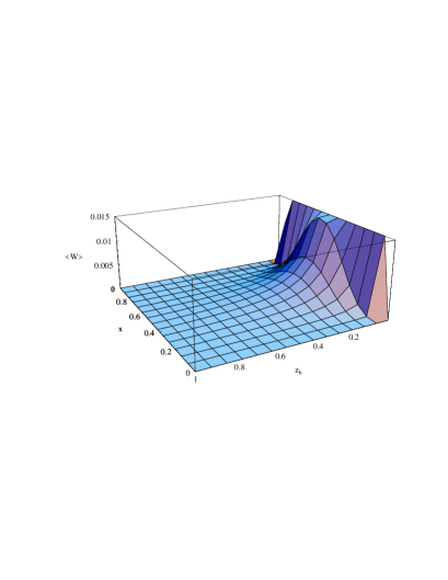
FIG. 4.: A three-dimensional view of $-\sum_{a,\bar{a}}e^{2}_{a}x_{B}h_{1L}^{\perp(1)a}(x_{B})H_{1}^{\perp(1)a}(z_{h})$, relevant for the $\sin(2\phi^{l}_{h})$ asymmetry in $\pi^{+}$ production, under the approximation $\tilde{h}_{L}(x)=\overline{h}_{L}=0$, as obtained by using the BBS set of distribution functions.

$\displaystyle\begin{array}[]{ll}\mbox{~{}\psfig{angle=0,width=213.39566pt}}&\mbox{~{}\psfig{angle=0,width=213.39566pt}}\end{array}$

FIG. 5.: A three-dimensional view of $-\sum_{a,\bar{a}}e^{2}_{a}\Bigl{[}x_{B}h_{1L}^{\perp(1)a}(x_{B})\tilde{H}^{a}(z_{h})/z-x_{B}^{2}h_{L}^{a}(x_{B})H_{1}^{\perp(1)a}(z_{h})\Bigr{]}$, relevant for the $\sin(\phi^{l}_{h})$ asymmetry in $\pi^{+}$ production, as obtained by using the BBS set of distribution functions, under the approximation $\tilde{h}_{L}=\overline{h}_{L}=0$ (on the left) and under the approximation $h_{1L}^{\perp(1)}(x)=0$ (on the right).

REFERENCES

• [1] HERMES Collaboration, A. Airapetian et al., hep-ex/9910062.
• [2] R.D. Tangerman and P.J. Mulders, Phys. Rev. D51 3357 (1995); P.J. Mulders and R.D. Tangerman, Nucl. Phys. B461 197 (1996).
• [3] D. Boer and P.J. Mulders, Phys. Rev. D57, 5780 (1998).
• [4] R.L. Jaffe and X. Ji, Nucl. Phys. B375, 527 (1992).
• [5] M. Boglione and P.J. Mulders, Phys. Rev. D60, 054007 (1999).
• [6] M. Anselmino, M. Boglione, F. Murgia, Phys. Rev. D60, 054027 (1999); M. Boglione and P.J. Mulders, Phys. Rev. D60, 054007 (1999).
• [7] M. Boglione and E. Leader, hep-ph/9911207.
• [8] D.L. Adams et al, Phys. Lett. B261, 201 (1991) and Phys. Lett. B264, 462 (1991).
• [9] A.V. Efremov, K. Goeke, M.V. Polyakov, D. Urbano, hep-ph/0001119.
• [10] J. Soffer, Phys. Rev. Lett. 74, 1292 (1995).
• [11] S.J. Brodsky, M. Burkhardt, I. Schmidt, Nucl. Phys. B441, 197 (1995).
• [12] E. Leader, A.V. Sidorov, D.B. Stamenov, Int. J. Mod. Phys. A13, No.32, 5573 (1998).
• [13] E. Leader, A.V. Sidorov, D.B. Stamenov, Phys. Lett. B462, 189 (1999).
• [14] A.D. Martin, R.G. Roberts, W.J. Stirling, R.S. Thorne, Eur. Phys. J. C4, 463 (1988).
• [15] A. Bacchetta, M. Boglione, A. Henneman, P.J. Mulders, hep-ph/9912490.
• [16] E. DeSanctis, W.-D. Nowak, K.A. Oganessyan, in preparation.
• [17] J. Binnewies, B.A. Kniehl, G. Kramer, Z. Phys. C64, 471 (1995).