IPNO-DR 99 23

CPT-99/P.3915

Contributions of order ${\cal O}(m_{\rm quark}^{2})$ to $K_{\ell 3}$ form factors and unitarity of the CKM matrix

N.H. Fuchs

Physics Department, Purdue University
West Lafayette IN 47907, USA

M. Knecht

Centre de Physique Théorique, CNRS-Luminy, Case 907
F-13288 Marseille Cedex 9, France

J. Stern

Groupe de Physique Théorique, Institut de Physique Nucléaire
F-91406 Orsay Cedex, France

The form factors for the $K_{\ell 3}$ semileptonic decay are computed to order $O(p^{4})$ in generalized chiral perturbation theory. The main difference with the standard $O(p^{4})$ expressions consists in contributions quadratic in quark masses, which are described by a single divergence-free low-energy constant, $A_{3}$. A new simultaneous analysis is presented for the CKM matrix element $V_{us}$, the ratio $F_{K}/F_{\pi}$, $K_{\ell 3}$ decay rates and the scalar form factor slope $\lambda_{0}$. This framework easily accommodates the precise value for $V_{ud}$ deduced from superallowed nuclear $\beta$-decays.

1 Introduction

Together with low-energy $\pi$–$\pi$ scattering [1, 2], the semi-leptonic $K_{\ell 3}$ [3] and $K_{e4}$ [4, 5] decays have been among the first applications of standard chiral perturbation theory (S$\chi$PT) [6, 2, 7] to be studied at the one-loop level. At this order, the mesonic form factors that describe these decays do not contain the poorly known low energy constants $L_{8}$ and $L_{6}$, and consequently they may be expected to be less sensitive to the size of the chiral condensate $\langle\bar{q}q\rangle$ than, e.g., the $\pi-\pi$ s-wave [8, 9]. In particular, the $K_{\ell 3}$ form factors at ${\cal O}({\rm p}^{4})$ merely involve, besides the masses and decay constants of the pseudoscalar states, the low energy constant $L_{9}$, whose value can be obtained [3] from the experimentally measured charge radius of the pion [10]. This fortunate circumstance has been used in the past to extract the CKM matrix element $V_{us}$ from the $K_{e3}$ decay rates [11], and presently this extraction is still considered by the Particle Data Group (PDG) compilation [12] to remain the most accurate and least model dependent. Yet this determination of $V_{us}$ relies on a model-dependent estimate of ${\cal O}(m_{\rm quark}^{2})$ contributions to the form factor $f_{+}(0)$ (the notation will be given below), which, in S$\chi$PT, arise as contributions of order ${\cal O}({\rm p}^{6})$. With the new careful and accurate determinations of $V_{ud}$ from superallowed nuclear $\beta$-decays [13, 14, 15], the size of these corrections is required to be comparable to the (parameter-free) genuine ${\cal O}({\rm p}^{4})$ contribution in order to preserve the unitarity of the CKM matrix. It is then legitimate to ask whether similarly important ${\cal O}(m_{\rm quark}^{2})$ contributions would not affect the parameter-free S$\chi$PT prediction for the slope $\lambda_{0}$ of the $K_{\mu 3}$ scalar form factor at order ${\cal O}({\rm p}^{4})$. In principle, these questions can be answered by performing the full two-loop S$\chi$PT calculation of the $K_{\ell 3}$ form factors, provided the several new ${\cal O}({\rm p}^{6})$ counterterms that will contribute can be measured independently or estimated in a reliable way . The present status of this enterprise is limited  to the evaluation of the so-called chiral double-logs [19], which, although only part of the full two-loop corrections, do not seem to point towards huge effects coming from the chiral loops themselves (see in particular the numerical results in Table 1 of Ref. [19] and the comments preceding it).

The purpose of the present work is to address some of these issues from the point of view of generalized chiral perturbation theory (G$\chi$PT) [8, 20, 21]. The expressions for the form factors of semileptonic decay of kaons to ${\cal O}({\rm p}^{4})$ in G$\chi$PT have never been published (a discussion of the $K_{\ell 4}$ form factors at order ${\cal O}({\rm p}^{2})$ in G$\chi$PT can be found in Ref. [22]), although they have existed for some time and have been partially reported on various occasions. Keeping in mind the well-known and important exception of the phase of the $K_{e4}^{+}$ decay amplitude, the $K_{\ell 3}$ and $K_{e4}$ form factors are indeed found to be to a large extent independent of the size of the condensate $\langle\bar{q}q\rangle$. The main consequence of the modified chiral counting ($m_{q}\sim{\cal O}({\rm p}))$ is that in G$\chi$PT the form factors receive a contribution quadratic in quark masses already at order ${\cal O}({\rm p}^{4})$, in addition to the standard ${\cal O}({\rm p}^{4})$ expressions. Furthermore, these new ${\cal O}(m_{\rm quark}^{2})$ contributions, which within S$\chi$PT would count as ${\cal O}({\rm p}^{6})$, are all related. They all stem from a single term of the ${\cal L}_{(2,2)}$ component of the effective Lagrangian ${\cal L}_{{\rm eff}}$ and they are described by a single divergence-free low-energy constant $A_{3}$ (see Ref. [9] and Appendix A for notation). (This statement is exact in the case of $K_{\ell 3}$ form factors $f_{+}$ and $f_{-}$, whereas in the case of $K_{e4}$ it remains true for the dominant ${\cal O}(m_{s}^{2})$ terms.) It thus appears that the ${\cal O}({\rm p}^{4})$ G$\chi$PT offers a predictive description of the terms quadratic in quark masses which is non-trivial compared to the one-loop S$\chi$PT (no quadratic terms) and yet much simpler than the standard ${\cal O}({\rm p}^{6})$ order, in which other unknown constants should contribute in addition to the ${\cal O}({\rm p}^{4})$ G$\chi$PT terms driven by the constant $A_{3}$. This framework, which is as systematic as the standard expansion, suggests a new simultaneous analysis of $V_{us}$, $K_{\ell 3}$ decay rates, $F_{K}/F_{\pi}$, and of the scalar slope $\lambda_{0}$ which may be of interest in connection with the constraint of unitarity of the CKM matrix and with the forthcoming new $K_{\ell 3}$ data. A closely related application, namely the determination of the ${\cal O}({\rm p}^{4})$ constant $L_{3}$ from the $K_{e4}^{0}$ decay rate, will be presented elsewhere [23], together with a full discussion of the $K_{\ell 4}$ form factors at order ${\cal O}({\rm p}^{4})$ in G$\chi$PT.

The present stage of our analysis involves one additional limitation, to the extent that no electromagnetic corrections are included, unless explicitly stated. For this reason we postpone a detailed analysis of the isospin asymmetry in the $K_{e3}^{0}$ and $K_{e3}^{+}$ decay rates that is due to the mass difference $m_{d}-m_{u}$. We just check that this asymmetry is consistent with the G$\chi$PT treatment of $\pi^{0}-\eta$ mixing within errors.

The paper is organized as follows: Section 2 provides the necessary expressions of the $K_{\ell 3}$ form factors and of the $\pi^{0}-\eta$ mixing angles in G$\chi$PT. Implications for the determinations of $V_{us}$ and of the ratio $F_{K}/F_{\pi}$ of pseudoscalar decay constants are discussed in Section 3. The slopes of the $K_{\ell 3}$ form factors are considered in Section 4. Concluding remarks are presented in Section 5. Details on the ${\cal O}({\rm p}^{4})$ structure of the G$\chi$PT effective Lagrangian and on its renormalization are presented in Appendix A. Useful expressions for the pseudoscalar masses and decay constants have been gathered in Appendix B.

2 $K_{\ell 3}$ form factors in G$\chi$PT to ${\cal O}({\rm p}^{4})$

We consider the two semileptonic decay channels

$$K^{+}(p) \rightarrow \pi^{0}(p^{\prime})\ell^{+}(p_{\ell})\nu_{\ell}(p_{\nu})\hskip 28.45274pt[K_{\ell 3}^{+}]$$

$$K^{0}(p) \rightarrow \pi^{-}(p^{\prime})\ell^{+}(p_{\ell})\nu_{\ell}(p_{\nu})\hskip 25.6073pt[K_{\ell 3}^{0}].$$ (2.1)

The symbol $\ell$ stands for $\mu$ or $e$. As stated before, we do not consider electromagnetic corrections. The processes (2.1) are then described by four form factors, $f^{K^{+}\pi^{0}}_{\pm}(t)$ and $f^{K^{0}\pi^{-}}_{\pm}(t)$, which depend on $t=(p^{\prime}-p)^{2}=(p_{l}+p_{\nu})^{2}$, the square of the four momentum transfer to the leptons, and which are defined in terms of the hadronic matrix elements of the charged strangeness changing QCD vector current as follows:

$$<\pi^{0}(p^{\prime})|({\overline{s}}\gamma_{\mu}u)(0)|K^{+}(p)> = \frac{1}{\sqrt{2}}\big{[}(p+p^{\prime})_{\mu}f^{K^{+}\pi^{0}}_{+}+(p-p^{\prime})_{\mu}f^{K^{+}\pi^{0}}_{-}\big{]}$$

$$<\pi^{-}(p^{\prime})|({\overline{s}}\gamma_{\mu}u)(0)|K^{0}(p)> = (p+p^{\prime})_{\mu}f^{K^{0}\pi^{-}}_{+}+(p-p^{\prime})_{\mu}f^{K^{0}\pi^{-}}_{-}.$$ (2.2)

2.1 G$\chi$PT expressions of the $K_{\ell 3}$ form factors

The one-loop G$\chi$PT expressions (using the notation of reference [3]) for the form factors are summarized below. We start with the two form factors $f^{K^{0}\pi^{-}}_{+}(t)$ and $f^{K^{+}\pi^{0}}_{+}(t)$, which are in practice sufficient for the description of the electron decay modes $K_{e3}^{+}$ and $K_{e3}^{0}$, and keeping isospin breaking contributions due to the quark mass difference $m_{d}-m_{u}$. For the $K_{\ell 3}^{0}$ channel, which is somewhat simpler, since $\pi^{0}-\eta$ mixing only enters the loop contributions, we obtain

$$f_{+}^{K^{0}\pi^{-}}(t) = 1\ +\ H_{\pi^{+}K^{0}}(t)\ +\ {1\over 2}\,H_{\pi^{0}K^{+}}(t)\ +\ {3\over 2}\,H_{\eta K^{+}}(t)$$ (2.3)

$$+ \sqrt{3}\,\stackrel{{\scriptstyle o}}{{\varepsilon}}\,\bigg{[}H_{\pi K}(t)\ -\ H_{\eta K}(t)\bigg{]}$$

$$+ \bigg{[}{1\over 8}{\widehat{m}}^{2}\,\xi^{2}\,+\,{1\over 2}{\widehat{m}}^{2}A_{3}\bigg{]}\,(r-1)^{2}\,\big{(}1+{1\over R}\big{)}\;,$$

with (the definitions of the loop functions $M_{PQ}^{\rm r}\,(t)$, $K_{PQ}(t)$ and $L_{PQ}\,(t)$ that we use below can be found in Ref. [7])

$$H_{PQ}(t)\ =\ {1\over{F_{\pi}^{2}}}\,\bigg{[}t\,M_{PQ}^{\rm r}\,(t)\ -\ L_{PQ}\,(t)\ +\ {2\over 3}\,L_{9}^{\rm r}\,t\,\bigg{]}\ .\\$$ (2.4)

Here $\stackrel{{\scriptstyle o}}{{\varepsilon}}$ denotes the leading order $\pi^{0}-\eta$ mixing angle,

$$\stackrel{{\scriptstyle o}}{{\varepsilon}}\ =\ {\sqrt{3}\over 4R}\bigg{[}1-{\Delta_{GMO}\over M_{\eta}^{2}-M_{\pi}^{2}}+{2\over 3}\,(r_{2}-r)\ {r-1\over r+1}\ {M_{\pi}^{2}\over M_{\eta}^{2}-M_{\pi}^{2}}\bigg{]}\;,\\$$ (2.5)

where

$$r \equiv m_{s}/{\widehat{m}}$$

$$r_{2} \equiv 2{M_{K}^{2}\over M_{\pi}^{2}}-1$$ (2.6)

$$\Delta_{GMO} \equiv 3M_{\eta}^{2}-4M_{K}^{2}+M_{\pi}^{2}\;.$$

We work only at first order in the quark mass difference $(m_{d}-m_{u})$, i.e. we consider only terms that are at most of order ${\cal O}(1/R)$ , where

$$R={m_{s}-{\widehat{m}}\over m_{d}-m_{u}}.\\$$ (2.7)

The lowest order S$\chi$PT value for the $\pi^{0}-\eta$ mixing angle, $\stackrel{{\scriptstyle o}}{{\varepsilon}}_{\rm st}={\sqrt{3}\over 4R}$, is recovered by dropping, in Eq. (2.5), the last two terms, which are counted as order ${\cal O}({\rm p}^{4})$ in S$\chi$PT. The $\xi^{2}$ and $A_{3}$ terms in Eq. (2.3) are ${\cal O}({\rm p}^{4})$ contributions in G$\chi$PT (see the detailed formulas for the effective Lagrangian in Appendix A), but are absent at this order in S$\chi$PT.

For the $K_{\ell 3}^{+}$ decay mode, we find

$$f_{+}^{K^{+}\pi^{0}}(t) = f_{+}^{K^{0}\pi^{-}}(t)\times\left\{1\ +\ {{\sqrt{3}}\over 2}(\varepsilon_{1}\ +\ \varepsilon_{2})\right.$$

$$\qquad-\left.\ {1\over\sqrt{3}}{\widehat{m}}^{2}\xi^{2}(r-1)^{2}\,\stackrel{{\scriptstyle o}}{{\varepsilon}}\ -\ {\widehat{m}}^{2}C_{2}^{P}(r-1)^{2}\,\bigg{[}{1\over R}\ +\ {{2\stackrel{{\scriptstyle o}}{{\varepsilon}}}\over{\sqrt{3}}}\bigg{]}\right\}\;,$$

where the $\pi^{0}-\eta$ mixing angles at order ${\cal O}({\rm p}^{4})$, $\varepsilon_{1}$, $\varepsilon_{2}$, are defined in section 2.2 below. Although the constant $C_{2}^{P}$ corresponds to a counterterm of ${\cal L}_{(2,2)}$ (see Eq. (A) in Appendix A) that violates the Zweig rule, it is not expected to be suppressed, since this violation occurs in the $0^{-}$ channel.

At zero momentum transfer, Eq. (2.3) gives

$$f_{+}^{K^{0}\pi^{-}}(0) = 1\ -\ {1\over{256\pi^{2}F_{\pi}^{2}}}\,\bigg{\{}2\,(M_{\pi^{+}}^{2}+M_{K^{0}}^{2})\,h_{0}\big{(}{{M_{\pi^{+}}^{2}}\over{M_{K^{0}}^{2}}}\big{)}$$

$$+\quad(M_{\pi^{0}}^{2}+M_{K^{+}}^{2})\,h_{0}\big{(}{{M_{\pi^{0}}^{2}}\over{M_{K^{+}}^{2}}}\big{)}+3\,(M_{K^{+}}^{2}+M_{\eta}^{2})\,h_{0}\big{(}{{M_{K^{+}}^{2}}\over{M_{\eta}^{2}}}\big{)}$$

$$+\quad 2\,\sqrt{3}\stackrel{{\scriptstyle o}}{{\varepsilon}}\,\bigg{[}(M_{\pi}^{2}+M_{K}^{2})\,h_{0}\big{(}{{M_{\pi}^{2}}\over{M_{K}^{2}}}\big{)}\,-\,(M_{K}^{2}+M_{\eta}^{2})\,h_{0}\big{(}{{M_{K}^{2}}\over{M_{\eta}^{2}}}\big{)}\bigg{]}\bigg{\}}$$

$$+ \bigg{[}{1\over 8}{\widehat{m}}^{2}\xi^{2}+{1\over 2}{\widehat{m}}^{2}A_{3}\bigg{]}\,(r-1)^{2}\,\left(1+{1\over R}\right)\ ,$$

with

$$h_{0}(x)\,=\,1\,+\,{{2x}\over{1-x^{2}}}\,\ln x\ .\\$$ (2.10)

To recover the expression at order ${\cal O}({\rm p}^{4})$ in S$\chi$PT [11, 3] for $f_{+}^{K^{0}\pi^{-}}(0)$, one replaces $\stackrel{{\scriptstyle o}}{{\varepsilon}}$ by the leading order S$\chi$PT value $\stackrel{{\scriptstyle o}}{{\varepsilon}}_{\rm st}$, and one simply drops the last line in Eq. (2.1). Notice that this last contribution is the only correction of order ${\cal O}({\rm p}^{4})$ that does not vanish in the large-$N_{c}$ limit of QCD. The fact that the ${\cal O}({\rm p}^{4})$ corrections to $f_{+}^{K^{0}\pi^{-}}(0)$ in S$\chi$PT vanish altogether in the large-$N_{c}$ limit might provide a natural explanation why contributions of the ${\cal O}({\rm p}^{6})$ counterterms could be comparatively sizeable.

The expressions of the form factors $f_{-}^{K^{0}\pi^{-}}(t)$ and $f_{-}^{K^{+}\pi^{0}}(t)$ are rather cumbersome if ${\cal O}(m_{d}-m_{u})$ effects are included. Since we do not need the latter in this case, we give only the common expression of these two form factors in the isospin limit, which is

$$f_{-}^{K\pi}(t) = {1\over 2}{\widehat{m}}\xi(r-1)\ -\ {1\over 4}{\widehat{m}}^{2}\xi^{2}(r-1)(r+3)\ -\ {\widehat{m}}^{2}\xi{\tilde{\xi}}(r-1)(r+2)$$

$$+ {1\over 2}{\widehat{m}}^{2}(A_{1}+B_{1})(r^{2}-1)\ +\ {1\over 2}{\widehat{m}}^{2}(A_{2}-2B_{2})(r-1)$$

$$+ {\widehat{m}}^{2}D^{S}(r-1)(r+2)\ +\ {1\over 4}[5\mu_{\pi}-2\mu_{K}-3\mu_{\eta}]$$

$$- {1\over{4F_{0}^{2}}}\,\big{[}5\,t-2\,M_{\pi}^{2}-2\,M_{K}^{2}+16{\widehat{m}}^{2}(A_{0}+2\,Z_{0}^{S})(r+1)\big{]}\,K_{\pi K}(t)$$

$$- {1\over{4F_{0}^{2}}}\,\big{[}3t-2M_{\pi}^{2}-2M_{K}^{2}+4{\widehat{m}}^{2}(A_{0}+2Z_{0}^{P})(r-1)(r+3)\big{]}\,K_{K\eta}(t)$$

$$- {3\over{2F_{0}^{2}}}\,(M_{K}^{2}-M_{\pi}^{2})\left\{\left[M_{K\pi}^{\rm r}\,(t)\,+\,{2\over 3}\,L_{9}^{\rm r}\right]\ +\ \left[M_{K\eta}^{\rm r}\,(t)\,+\,{2\over 3}\,L_{9}^{\rm r}\right]\right\}\;.$$

For the ease of comparison, we may rewrite this G$\chi$PT expression for the form factor $f_{-}(t)$ in terms of the corresponding S$\chi$PT expression:

$$f_{-}^{K\pi;std}(t) = \frac{F_{K}}{F_{\pi}}-1-\frac{2\,L_{9}^{r}\,\left(M_{K}^{2}-M_{\pi}^{2}\right)}{F_{\pi}^{2}}$$ (2.12)

$$+\,{\frac{\left(2\,M_{K}^{2}+2\,M_{\pi}^{2}-3\,t\right)}{4\,F_{\pi}^{2}}}\,K_{K\eta}(t)$$

$$+\,{\frac{\left(2\,M_{K}^{2}+2\,M_{\pi}^{2}-5\,t\right)}{4\,F_{\pi}^{2}}}\,K_{\pi K}(t)$$

$$-\,\frac{3\,\left(M_{K}^{2}-M_{\pi}^{2}\right)\,}{2\,F_{\pi}^{2}}\,\left[{M^{r}}_{K\eta}(t)+{M^{r}}_{K\pi}(t)\right]\;,$$

$$f_{-}^{K\pi}(t) = f_{-}^{K\pi;std}(t)$$ (2.13)

$$-\,\frac{1}{4}\left(\frac{F_{K}}{F_{\pi}}-1\right)^{2}\,\left({\frac{F_{K}^{2}}{{F_{\pi}}^{2}}}+2\frac{\,F_{K}}{F_{\pi}}-1\right)$$

$$-\,\frac{1}{2}\,{m^{2}}\,{A_{3}}\,(r-1)(r+3)$$

$$-\,{\frac{{\Delta_{GMO}}\,\left(r+3\right)}{4\,{F_{\pi}^{2}}\,\left(r-1\right)}}\,K_{K\eta}(t)-\frac{M_{\pi}^{2}\,\left(1+r\right)\,\hat{\epsilon}(r)}{F_{\pi}^{2}}\,K_{\pi K}(t)\;,$$

where

$$\hat{\epsilon}(r) \equiv {4\,{\widehat{m}}^{2}\,(A_{0}+2\,Z_{0}^{S})\over M_{\pi}^{2}}=2{r_{2}-r\over r^{2}-1}(1+2\zeta)$$

$$\zeta = Z_{0}^{S}/A_{0}\;,$$ (2.14)

and the ${\cal O}({\rm p}^{4})$ expression

$$\hat{m}\xi = {1\over r-1}\left({{F_{K}^{2}}\over{F_{\pi}^{2}}}-1\right)$$

$$-(r+1)\,\hat{m}^{2}\,(A_{1}+B_{1})-\hat{m}^{2}\,(A_{2}-2B_{2})-(r+3)\,\hat{m}^{2}\,A_{3}$$

$$-2\,(r+2)\,\hat{m}^{2}D^{S}$$

$$+2\,\hat{m}^{2}\,\xi^{2}+2\,(r+2)\,\hat{m}^{2}\xi\tilde{\xi}$$

$$-{1\over 2(r-1)}\,(5\mu_{\pi}-2\mu_{K}-3\mu_{\eta})$$

has been used. It is remarkable that, in Eq. (2.13), all ${\cal L}_{(2,2)}$ constants – except for $A_{3}$ – have been absorbed into the renormalization of the decay constants. Notice also that, in contrast to $f_{+}(t)$, $f_{-}(t)$ starts only at next-to-leading order in the chiral expansion, and that furthermore this contribution is not suppressed at $t=0$ for $N_{c}\to\infty$.

2.2 Mixing angles

The expressions of the $K_{\ell 3}$ form factors given in the preceding subsection involve the $\pi^{0}-\eta$ mixing angles $\stackrel{{\scriptstyle o}}{{\varepsilon}},\varepsilon_{1},\varepsilon_{2}$. In defining them we ignore isospin breaking through electromagnetic effects, so that the only source of isospin violation is the quark mass difference $m_{d}-m_{u}$. If $m_{d}\neq m_{u}$, the isosinglet and isovector axial currents $A_{\mu}^{8}$ and $A_{\mu}^{3}$ have nonvanishing off-diagonal matrix elements between the vacuum and one-meson states. The $two$ $\pi^{0}\-\eta$ mixing angles $\varepsilon_{1}$ and $\varepsilon_{2}$ are introduced such as to define combinations of the axial currents having vanishing off-diagonal matrix elements:

$$\langle\Omega|\,\cos\varepsilon_{1}\,A_{\mu}^{8}(0)-\sin\varepsilon_{1}\,A_{\mu}^{3}(0)\,|\pi^{0}(p)\rangle = 0$$

$$\langle\Omega|\,\cos\varepsilon_{2}\,A_{\mu}^{3}(0)+\sin\varepsilon_{2}\,A_{\mu}^{8}(0)\,|\eta(p)\rangle = 0.$$

Both $\varepsilon_{1}$ and $\varepsilon_{2}$ are of order ${\cal O}(m_{d}-m_{u})$. Note that we were not forced to define mixing angles in terms of matrix elements of the axial currents: we could have chosen to use the pseudoscalar densities, or any other operators with the appropriate quantum numbers; however, the corresponding expressions for the mixing angles would in general differ from those given below.

Keeping only contributions which are at most linear in the quark mass difference $m_{d}-m_{u}$, the off-diagonal matrix elements of the flavor neutral axial currents read

$$\langle\Omega|A_{\mu}^{8}(0)|\pi^{0}(p)\rangle = ip_{\mu}\,F_{\pi}\,\varepsilon_{1}$$

$$\langle\Omega|A_{\mu}^{3}(0)|\eta(p)\rangle = -ip_{\mu}\,F_{\eta}\,\varepsilon_{2}.$$

The decay constants $F_{\pi}$ and $F_{\eta}$ define the diagonal matrix elements of the same currents,

$$\langle\Omega|A_{\mu}^{3}(0)|\pi^{0}(p)\rangle = ip_{\mu}\,F_{\pi}$$

$$\langle\Omega|A_{\mu}^{8}(0)|\eta(p)\rangle = ip_{\mu}\,F_{\eta}\,\;.$$

Up to corrections of order ${\cal O}((m_{u}-m_{d})^{2})$ that we neglect, $F_{\pi}$ can be identified with the charged pion decay constant, $F_{\pi}$ = 92.4 MeV.

At order ${\cal O}({\rm p}^{2})$, the two mixing angles coincide and are equal to $\stackrel{{\scriptstyle o}}{{\varepsilon}}$. At order ${\cal O}({\rm p}^{3})$, they both receive ${\cal O}(m_{\rm quark})$ corrections, and are no longer equal. Explicitly,

$${\varepsilon_{1}\ +\ \varepsilon_{2}\over 2} = \stackrel{{\scriptstyle o}}{{\varepsilon}}\,+\,{1\over\sqrt{3}R(M_{\eta}^{2}-M_{\pi}^{2})}\,\bigg{\{}{\widehat{m}}^{3}X_{\rho}(r)$$ (2.19)

$$-\bigg{(}{F_{K}^{2}\over F_{\pi}^{2}}-1\bigg{)}\,\bigg{[}{\Delta_{GMO}\over 2}+{1\over 3}(r_{2}-r)\bigg{(}{r+2\over r+1}\bigg{)}M_{\pi}^{2}\bigg{]}\bigg{\}}\;,$$

and

$$\varepsilon_{1}-\varepsilon_{2} = \frac{1}{\sqrt{3}R(M_{\eta}^{2}-M_{\pi}^{2})}\left(\frac{F_{K}^{2}}{F_{\pi}^{2}}-1\right)\,\bigg{[}\Delta_{GMO}-\frac{2}{3}(r_{2}-r)\left(\frac{r-2}{r+1}\right)M_{\pi}^{2}\bigg{]}\;,$$ (2.20)

where we have defined

$$X_{\rho}(r)=(r-1)^{2}\,[(3\rho_{1}+4\rho_{3})\,(r-1)-\rho_{2}\,(r+1)]\\$$ (2.21)

in terms of the ${\cal L}_{(0,3)}$ quantities $\rho_{1,2,3}$.

3 Decay rates, $V_{us}$ and $F_{K}/F_{\pi}$ revisited

3.1 The $K^{0}\rightarrow\pi^{-}e^{+}\nu$ rate

For the $K_{e3}$ decay we only need to consider the form factor $f_{+}(t)$, and for $K^{0}\rightarrow\pi^{-}e^{+}\nu$ Eq. (2.3) is all we need. Ignoring the tiny term in Eq. (2.3) proportional to $\stackrel{{\scriptstyle o}}{{\varepsilon}}$, we may write the decay rate in units of $10^{-15}~{}{\mbox{\rm{MeV}}}$ as

$$\Gamma[K^{0}\rightarrow\pi^{-}e^{+}\nu] = V_{us}^{2}\bigg{[}105.056$$

$$+\,203.031\,(r-1)^{2}\,\bigg{(}\frac{{\widehat{m}}^{2}A_{3}}{2}+\frac{{\widehat{m}}^{2}\xi^{2}}{8}\bigg{)}$$

$$+\,98.267\,(r-1)^{4}\,\bigg{(}\frac{{\widehat{m}}^{2}A_{3}}{2}+\frac{{\widehat{m}}^{2}\xi^{2}}{8}\bigg{)}^{2}\bigg{]}.$$

Strictly speaking, the last contribution on the right-hand side of this expression, although coming from the square of the ${\cal O}({\rm p}^{4})$ expression of $f_{+}^{K^{0}\pi^{-}}(t)$, represents an order ${\cal O}({\rm p}^{6})$ effect in the chiral expansion of the decay rate. However, as can be checked e.g. on Figs. 1 and 2 below, it does not affect our analysis in the range of values considered for the Cabibbo angle.

We express ${\widehat{m}}\xi$ in terms of $V_{us}$ as follows: first, we use Eq. (2.1), but only at lowest order,

$${\widehat{m}}\xi={1\over r-1}\bigg{(}{F_{K}^{2}\over F_{\pi}^{2}}-1\bigg{)}\;,\\$$ (3.2)

and then use the formula for the ratio of the branching rates

$${\Gamma[K\rightarrow\mu\nu]\over\Gamma[\pi\rightarrow\mu\nu]}={\left|V_{us}\right|^{2}\over\left|V_{ud}\right|^{2}}{F_{K}^{2}\over F_{\pi}^{2}}{M_{K^{+}}\over M_{\pi^{+}}}{\left\{1-(M_{\mu}/M_{K^{+}})^{2}\right\}^{2}\over\left\{1-(M_{\mu}/M_{\pi^{+}})^{2}\right\}^{2}}\cdot(1+\delta_{K}-\delta_{\pi})\;,\\$$ (3.3)

where the radiative corrections $\delta_{K}=0.0020\pm 0.0002,\delta_{\pi}=0.0017\pm 0.0002$ nearly cancel [26].

Next, we use the experimental values [12] for the branching rates to fix [11] the combination of constants

$${F_{K}\over F_{\pi}}{V_{us}\over V_{ud}}=0.2758\pm 0.0005,\\$$ (3.4)

together with the unitarity of the Cabibbo-Kobayashi-Maskawa (CKM) matrix

$$V_{ud}^{2}+V_{us}^{2}=1.\\$$ (3.5)

We ignore $|V_{ub}|$, which has been obtained [27, 28] from a model-dependent analysis of data from B semileptonic decays to be (3.25 $\pm$ 0.6) $\times 10^{-3}$; however, even if the central value of $V_{ub}$ turned out to be three times larger, this would not affect our results. After expanding Eq. (LABEL:GammaK0) in $V_{us}$ around $V_{us}=0.220$, this implies

$$\Gamma[K^{0}\rightarrow\pi^{-}e^{+}\nu] = 5.390+31.10\,(V_{us}-0.220)$$ (3.6)

$$+\,(r-1)^{2}\,{\widehat{m}}^{2}A_{3}\,[5.059+37.58\,(V_{us}-0.220)]$$

$$+\,(r-1)^{4}\,{\widehat{m}}^{4}A_{3}^{2}\,[1.189+10.81\,(V_{us}-0.220)],$$

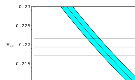
to be compared with the experimental rate of $4.937\pm 0.052$. Consequently, from the knowledge of $V_{us}$ one may extract a value for the ${\cal L}_{(2,2)}$ quantity ${\widehat{m}}^{2}(r-1)^{2}A_{3}=(m_{s}-{\widehat{m}})^{2}A_{3}$. For example, in Figure 1 we show the band in the ($V_{us}\,,\,A_{3}$) plane indicated by experiment, together with lines of constant $V_{us}$ corresponding to the Particle Data Group (PDG) [12] value $V_{us}=0.2196\pm 0.0023$. Accepting this constraint on $V_{us}$ would imply ${\widehat{m}}^{2}(r-1)^{2}A_{3}=-0.089\pm 0.024$. A naive dimensional analysis (NDA) [9] would give

$$|(r-1)^{2}\,{\widehat{m}}^{2}\,A_{3}|\,{\bigg{|}}_{NDA}\approx{m_{s}^{2}(\Lambda_{H})\over\Lambda_{H}^{2}}\approx 0.04\;,\\$$ (3.7)

where we have taken $m_{s}(\Lambda_{H})\approx$ 200 MeV, and $\Lambda_{H}\approx$ 1 GeV is a typical hadronic mass scale.

Figure 1: The dependence of $V_{us}$ on $A_{3}$. Horizontal lines indicate the range of values for $V_{us}$ given by PDG [12].

3.2 Determination of $V_{ud}$ from nuclear beta decay

In its 1998 update, PDG [12] recommends for $V_{us}$ only the value determined from $K_{e3}$ decay, arguing that the value obtained from hyperon decays (see [29] for an early attempt along these lines) suffers from theoretical uncertainties due to first-order SU(3) symmetry-breaking effects in the axial-vector couplings. However, within the context of the present G$\chi$PT analysis, we may not, without independent knowledge of $A_{3}$, use the values for $V_{us}$ thereby extracted from $K_{e3}$ decay. Moreover, $F_{K}$ is determined from the $K_{\mu 2}$ decay together with the knowledge of $V_{us}$, and we note that $F_{K}/F_{\pi}$ appears implicitly in our theoretical expressions for the $K_{\ell 3}$ form factors. The origin of this is, of course, our re-expression Eq. (3.2) of the ${\cal{L}}_{(0,3)}$ constant $\xi$ in terms of $F_{K}/F_{\pi}$.

¿From the unitarity condition for the CKM matrix, it follows that $|V_{us}|$ may be fixed from the knowledge of the up-down quark-mixing matrix element of the CKM matrix, $|V_{ud}|$, alone. The value of $V_{ud}$ can be determined from several independent sources: nuclear superallowed Fermi beta decays, free neutron decay, and pion beta decay.

Currently, superallowed Fermi $0^{+}\rightarrow 0^{+}$ nuclear beta decays [13, 14, 15], together with the muon lifetime, provide the most accurate value,

$$V_{ud}=0.9740\pm 0.0005.\\$$ (3.8)

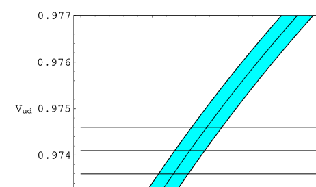
The precision is limited not by experimental error but by the estimated uncertainty in theoretical corrections [15]. In Figure 2 we show the band in the $V_{ud}\,,\,A_{3}$ plane indicated by experiment, together with lines of constant $V_{ud}$ corresponding to these values.

Figure 2: The dependence of $V_{ud}$ on $A_{3}$. Horizontal lines indicate the range of values for $V_{ud}$ determined from superallowed nuclear beta decay.

The determinations of $V_{ud}$ from free neutron decay data are approximately a factor of four poorer in precision (see the discussion in [15] and references therein),

$$V_{ud}=0.9759\pm 0.0021,\\$$ (3.9)

due to the difficulty in separating the vector from the axial piece, but planned experiments aiming at an accurate measurement of the electron emission asymmetry [30] could change this situation qualitatively, since the error in this case is primarily of experimental origin.

Finally, the theoretical corrections in the nuclear Fermi transitions are absent in the case of the pion beta decay. The present status of this type of experiments results in the value [15]

$$V_{ud}=0.9670\pm 0.0161.\\$$ (3.10)

Here also, the situation might improve in the future [31, 30].

Combining the above results, one obtains

$$V_{ud}=0.9741\pm 0.0005.\\$$ (3.11)

Accepting this value for $V_{ud}$ would imply ${\widehat{m}}^{2}(r-1)^{2}A_{3}=-0.124\pm 0.022$, somewhat larger than the NDA estimate Eq. (3.7), but still acceptable.

Finally, we note that recent (model-dependent) analyses of hyperon semileptonic decays give [32]

$$V_{ud}=0.9750\pm 0.0004,\\$$ (3.12)

and [33]

$$V_{ud}=0.9743\pm 0.0009.\\$$ (3.13)

Taking the value Eq. (3.11) for $V_{ud}$ (i.e., excluding results from hyperon decays), the unitarity relation Eq. (3.5) gives

$$V_{us}=0.2261\pm 0.0023.\\$$ (3.14)

Incorporating the above values for the CKM matrix elements into Eq. (3.4) then implies

$$\frac{F_{K}}{F_{\pi}}=1.189\pm 0.012\;\;\;[V_{ud}{\rm~{}from~{}nuclear~{}beta~{}decay]},\\$$ (3.15)

which may be compared with the corresponding result using the PDG values for $V_{us}$,

$$\frac{F_{K}}{F_{\pi}}=1.226\pm 0.014\;\;\;[V_{us}{\rm~{}from~{}PDG]}.\\$$ (3.16)

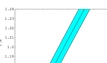
Using Eq. (3.4), which relates $F_{K}/F_{\pi}$ to $V_{us}$ and $V_{ud}$, Eq. (3.5) which relates $V_{us}$ and $V_{ud}$, and Eq. (3.6) which relates $V_{us}$ and ${\widehat{m}}^{2}(r-1)^{2}A_{3}$, we may directly relate $F_{K}/F_{\pi}$ and ${\widehat{m}}^{2}(r-1)^{2}A_{3}$, see Figure 3.

Figure 3: The dependence of $F_{K}/F_{\pi}$ on $A_{3}$.

3.3 $m_{u}\neq m_{d}$ effects on the $K^{+}\rightarrow\pi^{0}e^{+}\nu$ rate

We may treat the decay of the $K^{+}$ similarly; the result is most conveniently expressed in terms of the ratio

$${\Gamma[K^{+}\rightarrow\pi^{0}e^{+}\nu]\over\Gamma[K^{0}\rightarrow\pi^{-}e^{+}\nu]} = (R^{+0})^{2}\,\bigg{[}0.49615-0.00240\,(r-1)^{2}\,\bigg{(}\frac{{\widehat{m}}^{2}A_{3}}{2}+\frac{{\widehat{m}}^{2}\xi^{2}}{8}\bigg{)}$$

$$+\,0.00234\,(r-1)^{4}\,\bigg{(}\frac{{\widehat{m}}^{2}A_{3}}{2}+\frac{{\widehat{m}}^{2}\xi^{2}}{8}\bigg{)}^{2}\bigg{]},$$

where $R^{+0}$ is the ratio

$$R^{+0}\equiv{{\displaystyle f_{+}^{K^{+}\pi^{0}}(0)}\over{\displaystyle f_{+}^{K^{0}\pi^{-}}(0)}}\;.\\$$ (3.18)

Note that the last two terms in the brackets in Eq. (3.3) arise from the small differences in phase space which are due to mass differences between $K^{0}$ and $K^{+}$, and between $\pi^{+}$ and $\pi^{0}$.

Proceeding as we did for the $K^{0}$ rate above, i.e., using Eqs. (3.2) and (3.4), we obtain

$${\Gamma[K^{+}\rightarrow\pi^{0}e^{+}\nu]\over\Gamma[K^{0}\rightarrow\pi^{-}e^{+}\nu]} = (R^{+0})^{2}\,\big{\{}0.4961+0.0040\,(V_{us}-0.22)$$ (3.19)

$$-(r-1)^{2}\,{\widehat{m}}^{2}\,A_{3}\,[0.0011+0.0041\,(V_{us}-0.22)]$$

$$+0.0005\,(r-1)^{4}\,{\widehat{m}}^{4}\,A_{3}^{2}\big{\}}\;.$$

The correction terms in the curly brackets are completely negligible for $A_{3}$ and $V_{us}$ in the range determined above, since they are at most of the order of 0.0001, compared to the leading term 0.4961.

The measured rates may be deduced from the data given by the Particle Data Group [12]:

$$\Gamma[K^{+}\rightarrow\pi^{0}e^{+}\nu]_{exp} = 2.561\pm 0.032$$

$$\Gamma[K^{0}\rightarrow\pi^{-}e^{+}\nu]_{exp} = 4.937\pm 0.052,$$

where, as above, we express all rates in units of $10^{-15}$ MeV; consequently,

$${\Gamma[K^{+}\rightarrow\pi^{0}e^{+}\nu]_{exp}\over\Gamma[K^{0}\rightarrow\pi^{-}e^{+}\nu]_{exp}}=0.519\pm 0.016.\\$$ (3.21)

Consequently, the experimental value for $R^{+0}$ is 1.023 $\pm$ 0.016.

Up to and including terms of order ${\cal O}({\rm p}^{4})$, the theoretical expression for $R^{+0}$ is given by Eq. (2.1); the terms proportional to ${\widehat{m}}^{2}\xi^{2}(r-1)^{2}$ and to ${\widehat{m}}^{2}C_{2}^{P}$ are of order ${\cal O}({\rm p}^{4})$. We first estimate the ${\cal O}({\rm p}^{3})$ correction terms in Eq. (2.19) by NDA. For the first one, we obtain

$$\left|{{\widehat{m}}^{3}X_{\rho}(r)\over M_{\pi}^{2}}\right|_{NDA}\approx\left|{8\,r^{3}{\widehat{m}}^{3}\rho\over M_{\pi}^{2}}\right|_{NDA}\approx{8\,m_{s}^{3}(\Lambda_{H})\over M_{\pi}^{2}\Lambda_{H}}\approx 3.2,\\$$ (3.22)

where $\rho$ characterizes the size of the ${\cal L}_{(0,3)}$ low-energy constants $\rho_{\alpha},\,\alpha=1,2,3$. This implies (using $R=43.5$, from reference [24])

$${{\widehat{m}}^{3}X_{\rho}(r)\over R(M_{\eta}^{2}-M_{\pi}^{2})}\ \approx\ {0.22\over R}\ \approx\ 0.005.\\$$ (3.23)

Similarly, the last term in Eq. (2.19) is

$${1\over\sqrt{3}R(M_{\eta}^{2}-M_{\pi}^{2})}\bigg{(}{F_{K}^{2}\over F_{\pi}^{2}}-1\bigg{)}\,\bigg{[}{\Delta_{GMO}\over 2}+{1\over 3}(r_{2}-r)\bigg{(}{r+2\over r+1}\bigg{)}M_{\pi}^{2}\bigg{]}\quad$$

$$\approx\quad{-0.033\over R}+{0.006(r_{2}-r)\over R}\,\bigg{(}{r+2\over r+1}\bigg{)}$$ (3.24)

$$\qquad\approx\;-0.00075+0.00014\,(r_{2}-r)\,\bigg{(}{r+2\over r+1}\bigg{)}\;,$$

which is quite negligible.

Finally, we turn to the ${\cal O}({\rm p}^{4})$ corrections to $R^{+0}$. From

$${\widehat{m}}^{2}\xi^{2}(r-1)^{2}\approx\bigg{(}{F_{K}^{2}\over F_{\pi}^{2}}-1\bigg{)}^{2}\approx 0.24,\\$$ (3.25)

we obtain

$${{\widehat{m}}^{2}\xi^{2}(r-1)^{2}\stackrel{{\scriptstyle o}}{{\varepsilon}}\over\sqrt{3}}\approx 0.14\stackrel{{\scriptstyle o}}{{\varepsilon}}\;.\\$$ (3.26)

The NDA estimate for the $C_{2}^{P}$ term gives

$${\widehat{m}}^{2}\,\left|C_{2}^{P}\right|\,(r-1)^{2}\,\bigg{[}{1\over R}\ +\ {{2\stackrel{{\scriptstyle o}}{{\varepsilon}}}\over{\sqrt{3}}}\bigg{]}\approx 0.04\,\cdot\bigg{[}{1\over R}\ +\ {{2\stackrel{{\scriptstyle o}}{{\varepsilon}}}\over{\sqrt{3}}}\bigg{]}\;,\\$$ (3.27)

where we note that no assumption has been made here of any suppression of $C_{2}^{P}$ due to Zweig rule violation. We have verified that ${\cal O}({\rm p}^{4})$ corrections to $\varepsilon_{1}\ +\ \varepsilon_{2}$ are negligibly small. Using the numerical form of Eq. (2.5),

$$\stackrel{{\scriptstyle o}}{{\varepsilon}}\,=\,{1\over R}\,\bigg{[}0.533+0.502\,{r-1\over r+1}\,\bigg{(}1-{r\over r_{2}}\bigg{)}\bigg{]},\\$$ (3.28)

the upshot is that $R^{+0}$ may be written (recall Eq. (2.1))

$$R^{+0} = 1+\sqrt{3}\,\stackrel{{\scriptstyle o}}{{\varepsilon}}-\,0.14\,\stackrel{{\scriptstyle o}}{{\varepsilon}}\pm\,{0.22\over R}\;,$$ (3.29)

where the term $-0.14\,\stackrel{{\scriptstyle o}}{{\varepsilon}}$ comes from Eq. (3.26); the indicated uncertainty, coming from other higher-order corrections, is dominated by the estimation of the contributions from the ${\cal L}_{(0,3)}$ terms (see Eq. (3.23) above). Numerically, this implies

$$R^{+0}\,=\,1+{1\over R}\,\bigg{[}0.85+0.80\,{r-1\over r+1}\,\bigg{(}1-{r\over r_{2}}\bigg{)}\bigg{]}\pm{0.22\over R},\\$$ (3.30)

and taking, for example, the commonly accepted value [24] $R$ = 43.5 $\pm$ 2.2,

$$R^{+0}=1.020\pm 0.005\ +\ 0.018\,{r-1\over r+1}\,\bigg{(}1-{r\over r_{2}}\bigg{)},\\$$ (3.31)

which is consistent, for any permissible value of $r$, with the experimental value 1.023 $\pm$ 0.016 which we deduced above. In view of this experimental uncertainty, we will leave for a later time the careful investigation of the ${\cal O}({\rm p}^{4})$ effects mentioned above, together with the analysis of electromagnetic corrections (the radiative corrections to $R^{+0}$ in the standard case have been investigated in Ref. [34]). Note that some (but not all) of the existing experimental data has been published with radiative corrections, but often without mention of how these corrections have been implemented [35]. More precise knowledge of $R^{+0}$ would be useful in constraining the relationship displayed in Eq. (3.29) between the two quark-mass ratios $R$ and $r$, thereby testing the relevance of G$\chi$PT.

4 Form factor slopes

Analyses of $K_{\ell 3}$ data frequently assume a linear dependence

$$f^{K\pi}_{+,0}(t)=f^{K\pi}_{+}(0)\left[1+\lambda_{+,0}\frac{t}{M^{2}_{\pi^{+}}}\right]\;,\\$$ (4.1)

where, as usual, the scalar form factor is defined as

$$f^{K\pi}_{0}(t)=f^{K\pi}_{+}(t)+{t\over M_{K}^{2}-M_{\pi}^{2}}f^{K\pi}_{-}(t)\;.\\$$ (4.2)

The parameter $\lambda_{+}^{K\pi}$ is identical to that of S$\chi$PT,

$${\lambda_{+}^{K\pi}\over M_{\pi^{+}}^{2}} = {1\over 6}\,\langle\,{\rm r}^{2}\,\rangle^{\pi}_{\rm V}$$ (4.3)

$$+\ {1\over{64\pi^{2}F_{0}^{2}}}\,\bigg{[}1\,-\,{1\over 2}h_{1}\big{(}{{M_{\pi}^{2}}\over{M_{K}^{2}}}\big{)}\,-\,{1\over 2}h_{1}\big{(}{{M_{K}^{2}}\over{M_{\eta}^{2}}}\big{)}\,+\,{5\over 12}\ln\big{(}{{M_{\pi}^{2}}\over{M_{K}^{2}}}\big{)}\,+\,{1\over 4}\ln\big{(}{{M_{K}^{2}}\over{M_{\eta}^{2}}}\big{)}\bigg{]}\ ,$$

with

$$h_{1}(x)\ +\ {1\over 2}\,{{(x^{3}-3x^{2}-3x+1)}\over{(x-1)^{3}}}\,\ln x\,+\,{1\over 2}\,\left({{x+1}\over{x-1}}\right)^{2}\,-\,{1\over 3}\ ,\\$$ (4.4)

and

$$F_{\pi}^{2}\,\langle\,{\rm r}^{2}\,\rangle^{\pi}_{\rm V}\,\ =\,12\,L_{9}^{r}-\frac{1}{32\pi^{2}}\bigg{\{}2\ln\frac{M_{\pi}^{2}}{\mu^{2}}+\ln\frac{M_{K}^{2}}{\mu^{2}}+3\bigg{\}}\ .\\$$ (4.5)

On the other hand, the G$\chi$PT expression for $\lambda_{0}^{K\pi}$,

$${\lambda_{0}^{K\pi}\over M_{\pi^{+}}^{2}} = {1\over 2}\bigg{[}\left({{F_{K}^{2}}\over{F_{\pi}^{2}}}\,-\,1\right)\,-\,{1\over 2}\left({{F_{K}^{2}}\over{F_{\pi}^{2}}}\,-\,1\right)^{2}\,-\,{\widehat{m}}^{2}\,(r-1)^{2}\,A_{3}\,{r+3\over r-1}\bigg{]}{1\over M_{K}^{2}-M_{\pi}^{2}}$$

$$- {1\over{384\pi^{2}F_{0}^{2}}}\bigg{[}5\,-\,{{4M_{\pi}^{2}\,(r+1)\,\hat{\epsilon}(r)}\over{M_{K}^{2}+M_{\pi}^{2}}}\bigg{]}\,h_{2}\big{(}{{M_{\pi}^{2}}\over{M_{K}^{2}}}\big{)}$$

$$- {1\over{384\pi^{2}F_{0}^{2}}}\bigg{[}3\,+$$

$$\,2\,\left({{M_{\eta}^{2}-M_{K}^{2}}\over{M_{\eta}^{2}+M_{K}^{2}}}\right)\left({{M_{K}^{2}+M_{\pi}^{2}}\over{M_{K}^{2}-M_{\pi}^{2}}}\right)\left(1-{{\Delta_{GMO}\,(r+3)}\over{2\,(M_{K}^{2}+M_{\pi}^{2})\,(r-1)}}\right)\bigg{]}\,h_{2}\big{(}{{M_{K}^{2}}\over{M_{\eta}^{2}}}\big{)}$$

$$+ {1\over{64\pi^{2}F_{0}^{2}}}\ ,$$

where

$$h_{2}(x)\ =\ {3\over 2}\,\left({{1+x}\over{1-x}}\right)^{2}\,+\,{{3x(1+x)}\over{(1-x)^{3}}}\,\ln x\ ,\\$$ (4.7)

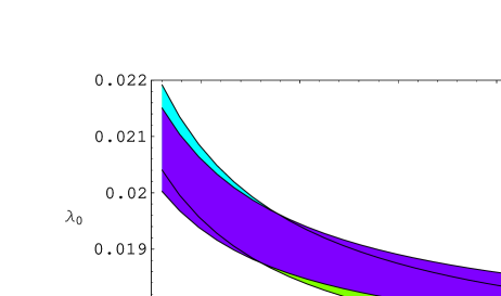
differs from the S$\chi$PT result. This expression for $\lambda_{0}$ explicitly displays the dependence on ${\widehat{m}}^{2}(r-1)^{2}A_{3}$ and on $r$, while its dependence on $V_{us}$ is implicit in the $F_{K}/F_{\pi}$ terms. However, as we saw above in Figure 3, $F_{K}/F_{\pi}$ and ${\widehat{m}}^{2}(r-1)^{2}A_{3}$ are correlated once we know the rate for $K^{0}\rightarrow\pi^{-}e^{+}\nu$. Therefore, for any choice of the quark mass ratio $r$, Eq. (4) gives a range of values for $\lambda_{0}$ corresponding to a given region in the ($F_{K}/F_{\pi},\ {\widehat{m}}^{2}(r-1)^{2}A_{3}$) plane. For example, Eq. (3.15) defines one region in Figure 3, while Eq. (3.16) defines another. We display in Figure 4 the corresponding regions in the ($\lambda_{0},r$) plane.

Figure 4: The dependence of $\lambda_{0}$ on $r$. The darker shaded region indicates the range of values Eq.  (3.15) for $\lambda_{0}$ determined by using $V_{ud}$ from superallowed nuclear beta decay, while the lighter shaded region shows the corresponding range Eq. (3.16) determined by using the PDG values for $V_{us}$. See text for details.

This analysis was done assuming that the Zweig-violating parameter $Z_{0}^{S}$=0. The whole dependence on $Z_{0}^{S}$ is contained (through $\zeta=Z_{0}^{S}/A_{0}$) in the parameter $\hat{\epsilon}(r)$. As pointed out in [21], the vacuum stability requirement $B_{0}\geq 0$ implies a upper bound on $\zeta$, which yields

$$\hat{\epsilon}(r)-\hat{\epsilon}(r)|_{\zeta=0}\ <\ (1-\hat{\epsilon}(r)|_{\zeta=0})\ {2\over r+2}\\$$ (4.8)

We find that taking $\zeta=0$ or its maximal allowed value makes a difference of less than 0.0004 in $\lambda_{0}$, for any choice of $r$.

In S$\chi$PT, including one-loop corrections, the result [3] is

$$\lambda_{0}=0.017\pm 0.004,\\$$ (4.9)

where the error is an estimate of the uncertainties due to higher-order contributions. The experimental situation remains unclear, in view of the inconsistency between some more recent data [12] and the result ($\lambda_{0}=0.019\pm 0.004$) of the high-statistics experiment of Donaldson et al [36].

5 Summary and discussion

In the preceding pages, we have studied the $K_{\ell 3}$ form factors at ${\cal O}({\rm p}^{4})$ precision within the generalized framework of chiral perturbation theory. In this connection, three (related) issues have been discussed: the extraction of the CKM matrix element $V_{us}$ from the experimental value of the $K_{\ell 3}$ branching ratios, the determination of the ratio $F_{K}/F_{\pi}$ of pseudoscalar decay constants, and the prediction for the slope $\lambda_{0}$ of the scalar form factor.

In the Leutwyler-Roos analysis [11], the expression of $f_{+}^{K^{0}\pi^{-}}(0)$ is written as

$$f_{+}^{K^{0}\pi^{-}}(0)=1+f_{1}+f_{2}+\cdots\,,\\$$ (5.1)

where the contributions $f_{1}$ and $f_{2}$ are of order $m_{\rm quark}$ and $m_{\rm quark}^{2}$ respectively. The one-loop S$\chi$PT contribution $f_{1}$ arises from Goldstone boson loops only, a counterterm contribution at this order of the standard counting being forbidden by the Ademollo-Gatto theorem. This leads to a parameter free prediction $f_{1}=-0.023$. Furthermore, $f_{2}$, which would arise at chiral order ${\cal O}({\rm p}^{6})$ in S$\chi$PT, has been estimated in [11] to be $-$0.016 $\pm$ 0.008 by using a model for pion and kaon wave functions to compute matrix elements in the infinite momentum frame. This leads to a value $V_{us}=0.2196\pm 0.0023$. Assuming unitarity of the CKM matrix in a three generation standard model, and using the existing estimates of $|V_{ub}|$, the determination $V_{ud}=0.9741\pm 0.0005$ from superallowed nuclear $\beta$-decays leads instead to $V_{us}=0.2261\pm 0.0022$. Therefore, unitarity of the CKM matrix can only be restored at the expense of having the S$\chi$PT two-loop correction $f_{2}$ at least as large as the one-loop contribution $f_{1}$. This is far from signaling a failure of the chiral expansion in the present case, since $f_{1}$ might be anomalously small, being, for instance, suppressed, even compared to $f_{2}$, in the large-$N_{c}$ limit (another consequence of the Ademollo-Gatto theorem). In G$\chi$PT, the corresponding expansion of $f_{+}^{K^{0}\pi^{-}}(0)$ reads

$$f_{+}^{K^{0}\pi^{-}}(0)=1+{\tilde{f}}_{1}+{\tilde{f}}_{2}+\cdots\,,\\$$ (5.2)

where ${\tilde{f}}_{1}$ collects all ${\cal O}({\rm p}^{4})$ contributions in the generalized chiral counting, and contains ${\cal O}(m_{\rm quark}^{2})$ terms. The difference between ${\tilde{f}}_{1}$ and $f_{1}$

$${\tilde{f}}_{1}-f_{1}=\bigg{[}{1\over 8}{\widehat{m}}^{2}\,\xi^{2}\,+\,{1\over 2}{\widehat{m}}^{2}A_{3}\bigg{]}\,(r-1)^{2}\,\big{(}1+{1\over R}\big{)}\;,\\$$ (5.3)

involves a single low-energy constant from ${\cal L}_{(2,2)}$, $A_{3}$, which would appear only at order ${\cal O}({\rm p}^{6})$ in S$\chi$PT. The contribution of the ${\cal L}_{(2,1)}$ low-energy constant $\xi$ is determined by the value of the ratio $F_{K}/F_{\pi}$. The value of $V_{ud}$ from the nuclear $\beta$-decay data can be accommodated by

$$(r-1)^{2}{\widehat{m}}^{2}A_{3}=-0.124\pm 0.022\,,\quad\frac{F_{K}}{F_{\pi}}=1.189\pm 0.012\,.\\$$ (5.4)

The corresponding difference is ${\tilde{f}}_{1}-f_{1}=-0.04\pm 0.01$, and it represents the value which would be required in the Leutwyler-Roos analysis for the two-loop contribution $f_{2}$ (instead of the estimate $f_{2}=-0.016\pm 0.008$ of [11]) in order to maintain the unitarity of the CKM matrix. Of course, a confirmation, with a comparable accuracy, from other sources (neutron decay, pion $\beta$-decay) of the value of $V_{ud}$ obtained from nuclear $\beta$-decays can only be welcome.

This determination of $A_{3}$ and the decrease in the value of the ratio of decay constants, as compared to the number $F_{K}/F_{\pi}=1.22\pm 0.01$ [11], is compatible with the present experimental information concerning the difference in the $K^{0}_{e3}$ and $K^{+}_{e3}$ decay rates, and induces only a mild modification in the prediction for the slope of the scalar form factor $\lambda_{0}$, which, as a function of the quark mass ratio $m_{s}/{\widehat{m}}$, varies between 0.0018 and 0.0022, well within the range set by the high-statistics $K^{0}_{L}$ experiment of Donaldson et al. [36]. The higher values of $\lambda_{0}$ obtained by some of the more recent experiments [12] are therefore difficult to understand at the theoretical level, and cannot be ascribed, within G$\chi$PT, to the manifestation of a smaller value of the bilinear light quark condensate.

We thus conclude that the nuclear $\beta$-decay determination of $V_{ud}=0.9741\pm 0.0005$ need not be in contradiction with the present values of the $K_{e3}$ decay rates and with chiral perturbation theory. One should then ask how the corresponding increase of $|V_{us}|$ by about 2.5 standard deviations would manifest itself in various observables. We have already mentioned that the present understanding of hyperon semi-leptonic decays is compatible with the suggested update of $V_{us}$. The effect on the $K_{e4}$ decay rates should be analyzed separately [23]. Some effect on the extraction of the ${\cal O}({\rm p}^{4})$ low-energy constants $L_{1},L_{2}$ and $L_{3}$ is to be expected a priori, but a precise statement requires a closer analysis. Finally, it is worth mentioning the possible effect on hadronic spectral functions which are extracted from the decays $\tau\rightarrow{\rm hadrons}+\nu_{\tau}$ and used for a determination of fundamental QCD parameters [38, 39, 40]. While the non-strange ($\bar{u}d$) spectral functions should be only barely affected by an increase of $\sim 0.25\%$, the recently published [40] strange ($\bar{u}s$) spectral functions should be reduced by $\sim 4.6\%$. Consequently, we would expect no notable influence on the determination of $\alpha_{S}(M_{\tau}^{2})$ [38], whereas the central value of the running strange quark mass ${\rm m_{s}}$ determined recently [39, 40] could increase by $\sim 15-20\%$. The issue certainly deserves a more detailed study.

Acknowledgments

Useful correspondence with W.S. Woolcock, W.C. Haxton and J. Comfort is kindly acknowledged. We also thank N. Vinh Mau for clarifying discussions.

Appendices

A Expansion and renormalization of the effective Lagrangian

In this Appendix, we display the structure of the effective action of G$\chi$PT up to order ${\cal O}({\rm p}^{4})$. For a general discussion of the G$\chi$PT expansion framework, we refer the reader to the existing literature [8, 20, 21].

At leading order, the generalized expansion is described by ${\tilde{\cal L}}^{(2)}$, which was first given in Ref. [8]:

$${\tilde{\cal L}}^{(2)} = {1\over 4}F_{0}^{2}\left\{\langle D_{\mu}U^{+}D^{\mu}U\rangle+2B_{0}\langle U^{+}\chi+\chi^{+}U\rangle\right.$$

$$\qquad+A_{0}\langle(U^{+}\chi)^{2}+(\chi^{+}U)^{2}\rangle+Z_{0}^{S}\langle U^{+}\chi+\chi^{+}U\rangle^{2}$$

$$\qquad+Z_{0}^{P}\langle U^{+}\chi-\chi^{+}U\rangle^{2}+\left.H_{0}\langle\chi^{+}\chi\rangle\right\}\ .$$

The notation is as in Refs. [7, 3], except for the consistent removal of the factor $2B_{0}$ from $\chi$, the parameter that collects the scalar and pseudoscalar sources,

$$\chi={s}+i{p}={\cal M}+\cdots\ ,\,{\cal M}={\rm diag}(m_{u},m_{d},m_{s})\ .\\$$ (A.6)

In G$\chi$PT, the next-to-leading-order corrections are of order ${\cal O}({\rm p}^{3})$, and still occur at tree level only. They are embodied in ${\tilde{\cal L}}^{(3)}={\cal L}_{(2,1)}+{\cal L}_{(0,3)}$, which reads [20, 37]

$$\tilde{\cal L}^{(3)} = {1\over 4}F_{0}^{2}\left\{\xi\langle D_{\mu}U^{+}D^{\mu}U(\chi^{+}U+U^{+}\chi)\rangle+\tilde{\xi}\langle D_{\mu}U^{+}D^{\mu}U\rangle\langle\chi^{+}U+U^{+}\chi\rangle\right.$$

$$\qquad+\rho_{1}\langle(\chi^{+}U)^{3}+(U^{+}\chi)^{3}\rangle+\rho_{2}\langle(\chi^{+}U+U^{+}\chi)\chi^{+}\chi\rangle$$

$$\qquad+\rho_{3}\langle\chi^{+}U-U^{+}\chi\rangle\langle(\chi^{+}U)^{2}-(U^{+}\chi)^{2}\rangle$$

$$\qquad+\rho_{4}\langle(\chi^{+}U)^{2}+(U^{+}\chi)^{2}\rangle\langle\chi^{+}U+U^{+}\chi\rangle$$

$$\qquad+\rho_{5}\langle\chi^{+}\chi\rangle\langle\chi^{+}U+U^{+}\chi\rangle$$

$$\qquad+\left.\rho_{6}\langle\chi^{+}U-U^{+}\chi\rangle^{2}\langle\chi^{+}U+U^{+}\chi\rangle+\rho_{7}\langle\chi^{+}U+U^{+}\chi\rangle^{3}\right\}\ .$$

The tree-level contributions at order ${\cal O}({\rm p}^{4})$ are contained in

$$\tilde{\cal L}^{(4)}={\cal L}_{(4,0)}+{\cal L}_{(2,2)}+{\cal L}_{(0,4)}+B_{0}^{2}{\cal L}^{\prime}_{(0,2)}+B_{0}{\cal L}^{\prime}_{(2,1)}+B_{0}{\cal L}^{\prime}_{(0,3)}\ .\\$$ (A.8)

The part without explicit chiral symmetry breaking, ${\cal L}_{(4,0)}$, is described by the same low-energy constants $L_{1}$, $L_{2}$, $L_{3}$, $L_{9}$ and $L_{10}$ as in S$\chi$PT [7]:

$${\cal L}_{(4,0)} = L_{1}\langle D_{\mu}U^{+}D^{\mu}U\rangle\langle D_{\nu}U^{+}D^{\nu}U\rangle+L_{2}\langle D_{\mu}U^{+}D^{\nu}U\rangle\langle D_{\mu}U^{+}D^{\nu}U\rangle$$

$$+L_{3}\langle D_{\mu}U^{+}D^{\mu}UD_{\nu}U^{+}D^{\nu}U\rangle-iL_{9}\langle F_{\mu\nu}^{R}D^{\mu}UD^{\nu}U^{+}+F_{\mu\nu}^{L}D^{\mu}U^{+}D^{\nu}U\rangle$$

$$+L_{10}\langle U^{+}F_{\mu\nu}^{R}UF^{L\mu\nu}\rangle+H_{1}\langle F_{\mu\nu}^{R}F^{R\mu\nu}+F_{\mu\nu}^{L}F^{L\mu\nu}\rangle\;.$$

The new term ${\cal L}_{(2,2)}$ would count as ${\cal O}({\rm p}^{6})$ in S$\chi$PT, and is given by:

$${\cal L}_{(2,2)} = {1\over{4}}F_{0}^{2}\left\{A_{1}\langle D_{\mu}U^{+}D^{\mu}U(\chi^{+}\chi+U^{+}\chi\chi^{+}U)\rangle\right.$$

$$\qquad+A_{2}\langle D_{\mu}U^{+}U\chi^{+}D^{\mu}UU^{+}\chi\rangle$$

$$\qquad+A_{3}\langle D_{\mu}U^{+}U(\chi^{+}D^{\mu}\chi-D^{\mu}\chi^{+}\chi)+D_{\mu}UU^{+}(\chi D^{\mu}\chi^{+}-D^{\mu}\chi\chi^{+})\rangle$$

$$\qquad+A_{4}\langle D_{\mu}U^{+}D^{\mu}U\rangle\langle\chi^{+}\chi\rangle$$

$$\qquad+B_{1}\langle D_{\mu}U^{+}D^{\mu}U(\chi^{+}U\chi^{+}U+U^{+}\chi U^{+}\chi)\rangle$$

$$\qquad+B_{2}\langle D_{\mu}U^{+}\chi D^{\mu}U^{+}\chi+\chi^{+}D_{\mu}U\chi^{+}D^{\mu}U\rangle$$

$$\qquad+B_{3}\langle U^{+}D_{\mu}\chi U^{+}D^{\mu}\chi+D_{\mu}\chi^{+}UD^{\mu}\chi^{+}U\rangle$$

$$\qquad+B_{4}\langle D_{\mu}U^{+}D^{\mu}U\rangle\langle\chi^{+}U\chi^{+}U+U^{+}\chi U^{+}\chi\rangle$$

$$\qquad+C_{1}^{S}\langle D_{\mu}U\chi^{+}+\chi D^{\mu}U^{+}\rangle\langle D_{\mu}U\chi^{+}+\chi D^{\mu}U^{+}\rangle$$

$$\qquad+C_{2}^{S}\langle D_{\mu}\chi^{+}U+U^{+}D^{\mu}\chi\rangle\langle D_{\mu}U^{+}\chi+\chi^{+}D^{\mu}U\rangle$$

$$\qquad+C_{3}^{S}\langle D_{\mu}\chi^{+}U+U^{+}D^{\mu}\chi\rangle\langle D_{\mu}\chi^{+}U+U^{+}D^{\mu}\chi\rangle$$

$$\qquad+C_{1}^{P}\langle D_{\mu}U\chi^{+}-\chi D^{\mu}U^{+}\rangle\langle D_{\mu}U\chi^{+}-\chi D^{\mu}U^{+}\rangle$$

$$\qquad+C_{2}^{P}\langle D_{\mu}\chi^{+}U-U^{+}D^{\mu}\chi\rangle\langle D_{\mu}U^{+}\chi-\chi^{+}D^{\mu}U\rangle$$

$$\qquad+C_{3}^{P}\langle D_{\mu}\chi^{+}U-U^{+}D^{\mu}\chi\rangle\langle D_{\mu}\chi^{+}U-U^{+}D^{\mu}\chi\rangle$$

$$\qquad+D^{S}\langle D_{\mu}U^{+}D^{\mu}U(\chi^{+}U+U^{+}\chi)\rangle\langle\chi^{+}U+U^{+}\chi\rangle$$

$$\qquad+D^{P}\langle D_{\mu}U^{+}D^{\mu}U(\chi^{+}U-U^{+}\chi)\rangle\langle\chi^{+}U-U^{+}\chi\rangle$$

$$\qquad+\left.H_{2}\langle D_{\mu}\chi^{+}D^{\mu}\chi\rangle\right\}\;.$$

Notice that the number of counterterms (17) involved in ${\cal L}_{(2,2)}$ agrees with Refs. [16, 17]. However, in both cases, different bases have been used. Finally, the tree-level contributions which behave as ${\cal O}(m_{\rm quark}^{4})$ in the chiral limit are contained in ${\cal L}_{(0,4)}$,

$${\cal L}_{(0,4)} = {1\over{4}}F^{2}_{0}\left\{E_{1}\langle(\chi^{+}U)^{4}+(U^{+}\chi)^{4}\rangle\right.$$

$$\qquad+E_{2}\langle\chi^{+}\chi(\chi^{+}U\chi^{+}U+U^{+}\chi U^{+}\chi)\rangle$$

$$\qquad+E_{3}\langle\chi^{+}\chi U^{+}\chi\chi^{+}U\rangle$$

$$\qquad+F_{1}^{S}\langle\chi^{+}U\chi^{+}U+U^{+}\chi U^{+}\chi\rangle^{2}$$

$$\qquad+F_{2}^{S}\langle(\chi^{+}U)^{3}+(U^{+}\chi)^{3}\rangle\langle\chi^{+}U+U^{+}\chi\rangle$$

$$\qquad+F_{3}^{S}\langle\chi^{+}\chi(\chi^{+}U+U^{+}\chi)\rangle\langle\chi^{+}U+U^{+}\chi\rangle$$

$$\qquad+F_{4}^{S}\langle(\chi^{+}U)^{2}+(U^{+}\chi)^{2}\rangle\langle\chi^{+}\chi\rangle$$

$$\qquad+F_{1}^{P}\langle\chi^{+}U\chi^{+}U-U^{+}\chi U^{+}\chi\rangle^{2}$$

$$\qquad+F_{2}^{P}\langle(\chi^{+}U)^{3}-(U^{+}\chi)^{3}\rangle\langle\chi^{+}U-U^{+}\chi\rangle$$

$$\qquad+F_{3}^{P}\langle\chi^{+}\chi(\chi^{+}U-U^{+}\chi)\rangle\langle\chi^{+}U-U^{+}\chi\rangle$$

$$\qquad+F_{5}^{SS}\langle(\chi^{+}U)^{2}+(U^{+}\chi)^{2}\rangle\langle\chi^{+}U+U^{+}\chi\rangle^{2}$$

$$\qquad+F_{6}^{SS}\langle\chi^{+}\chi\rangle\langle\chi^{+}U+U^{+}\chi\rangle^{2}$$

$$\qquad+F_{5}^{SP}\langle(\chi^{+}U)^{2}+(U^{+}\chi)^{2}\rangle\langle\chi^{+}U-U^{+}\chi\rangle^{2}$$

$$\qquad+F_{6}^{SP}\langle\chi^{+}\chi\rangle\langle\chi^{+}U-U^{+}\chi\rangle^{2}$$

$$\qquad+F_{7}^{SP}\langle(\chi^{+}U)^{2}-(U^{+}\chi)^{2}\rangle\langle\chi^{+}U-U^{+}\chi\rangle\langle\chi^{+}U+U^{+}\chi\rangle$$

$$\qquad+\left.H_{3}\langle\chi^{+}\chi\chi^{+}\chi\rangle+H_{4}\langle\chi^{+}\chi\rangle^{2}\right\}\;.$$

Contributions from ${\cal L}_{(0,4)}$ would only appear at order ${\cal O}({\rm p}^{8})$ in S$\chi$PT, which, to the best of our knowledge, have not been discussed in the literature.

The ${\cal O}({\rm p}^{4})$ loop corrections to the processes studied here involve only graphs with one or two vertices from ${\tilde{\cal L}}^{(2)}$:

$${\tilde{\cal Z}}^{(4)}_{\rm 1\,loop}={\tilde{\cal Z}}^{(4)}_{\rm tadpole}+{\tilde{\cal Z}}^{(4)}_{\rm unitarity}+\cdots\\$$ (A.12)

The divergent parts of these one-loop graphs have been subtracted at a scale $\mu$ in the same dimensional renormalization scheme as described in [7]. Accordingly, the low energy constants of ${\cal L}_{(4,0)}$, ${\cal L}_{(2,2)}$, and ${\cal L}_{(0,4)}$ stand for the renormalized quantities, with an explicit logarithmic scale dependence ($X(\mu)$ denotes generically any of these renormalized low-energy constants)

$$X(\mu)=X(\mu^{\prime})+{{\Gamma_{X}}\over{(4\pi)^{2}}}\,\cdot\ln({\mu^{\prime}}/\mu)\ .\\$$ (A.13)

At order ${\cal O}({\rm p}^{4})$, the low-energy constants of ${\tilde{\cal L}}^{(2)}$ and ${\tilde{\cal L}}^{(3)}$ also need to be renormalized. The corresponding counterterms, however, are of order ${\cal O}(B_{0}^{2})$ and ${\cal O}(B_{0})$, respectively, and they are gathered in the three last terms of Eq. (A.8): in G$\chi$PT, renormalization proceeds order by order in the expansion in powers of $B_{0}$ [20, 21]. Alternatively, one may think of Eqs. (A) and (A) as standing for the combinations ${\tilde{\cal L}}^{(2)}+B_{0}^{2}{\cal L}^{\prime}_{(0,2)}$ and ${\tilde{\cal L}}^{(3)}+B_{0}{\cal L}^{\prime}_{(2,1)}+B_{0}{\cal L}^{\prime}_{(0,3)}$, respectively, with the corresponding low-energy constants representing the renormalized quantities. The full list of $\beta$-function coefficients $\Gamma_{X}$ are tabulated below.

$X$	$F_{0}^{2}\cdot\Gamma_{X}$
$A_{0}$	$5B_{0}^{2}/3$
$Z_{0}^{S}$	$11B_{0}^{2}/9$
$Z_{0}^{P}$	$0$
$H_{0}$	$10B_{0}^{2}/3$

Table 1: Subtraction scale dependences of the low energy constants of ${\tilde{\cal L}}^{(2)}$.

$X$	$F_{0}^{2}\cdot\Gamma_{X}$
$\xi$	$3B_{0}$
${\tilde{\xi}}$	$B_{0}$
$\rho_{1}$	$4B_{0}\left(\frac{1}{6}A_{0}+Z_{0}^{S}+Z_{0}^{P}\right)$
$\rho_{2}$	$4B_{0}\left(\frac{1}{6}A_{0}-Z_{0}^{S}+3Z_{0}^{P}\right)$
$\rho_{3}$	$4B_{0}\left({1\over 2}A_{0}-{2\over 3}Z_{0}^{S}+{5\over 6}Z_{0}^{P}\right)$
$\rho_{4}$	$4B_{0}\left({11\over 9}A_{0}+{5\over 6}Z_{0}^{S}-{2\over 3}Z_{0}^{P}\right)$
$\rho_{5}$	$4B_{0}\left(A_{0}+{5\over 3}Z_{0}^{S}-{4\over 3}Z_{0}^{P}\right)$
$\rho_{6}$	$4B_{0}\left({1\over 9}Z_{0}^{S}+{11\over 18}Z_{0}^{P}\right)$
$\rho_{7}$	$4B_{0}\left({11\over 18}Z_{0}^{S}+{1\over 9}Z_{0}^{P}\right)$

Table 2: Subtraction scale dependences of the low energy constants of ${\tilde{\cal L}}^{(3)}$.

$X$	$\Gamma_{X}$
$L_{1}$	${3\over{32}}$
$L_{2}$	${3\over{16}}$
$L_{3}$	$0$
$L_{9}$	${1\over{4}}$
$L_{10}$	$-{1\over{4}}$
$H_{1}$	$-{1\over{8}}$

Table 3: Subtraction scale dependences of the low energy constants of ${\cal L}_{(4,0)}$.

$X$	$F_{0}^{2}\cdot\Gamma_{X}$
$A_{1}$	$-6(Z_{0}^{S}-Z_{0}^{P})$
$A_{2}$	$0$
$A_{3}$	$0$
$A_{4}$	$2(Z_{0}^{S}-Z_{0}^{P})$
$B_{1}$	$(3A_{0}-2Z_{0}^{S}-2Z_{0}^{P})$
$B_{2}$	$4(Z_{0}^{S}+Z_{0}^{P})$
$B_{3}$	$0$
$B_{4}$	$(A_{0}+Z_{0}^{S}+Z_{0}^{P})$
$C_{1}^{S}$	$(A_{0}-2Z_{0}^{P})$
$C_{2}^{S}$	$0$
$C_{3}^{S}$	$0$
$C_{1}^{P}$	$(A_{0}-2Z_{0}^{S})$
$C_{2}^{P}$	$0$
$C_{3}^{P}$	$0$
$D^{S}$	$(A_{0}+7Z_{0}^{S})$
$D^{P}$	$(A_{0}+7Z_{0}^{P})$
$H_{2}$	$0$

Table 4: Subtraction scale dependences of the low energy constants of ${\cal L}_{(2,2)}$.

$X$	$F_{0}^{2}\cdot\Gamma_{X}$
$E_{1}$	$-{7\over 3}A_{0}^{2}+8A_{0}(Z_{0}^{S}+Z_{0}^{P})+{34\over 3}(Z_{0}^{S}+Z_{0}^{P})^{2}$
$E_{2}$	$-16A_{0}(Z_{0}^{S}-Z_{0}^{P})+24(Z_{0}^{S})^{2}-24(Z_{0}^{P})^{2}$
$E_{3}$	$-{14\over 3}A_{0}^{2}+8A_{0}(Z_{0}^{S}+Z_{0}^{P})+{8\over 9}\left[35(Z_{0}^{S})^{2}+35(Z_{0}^{P})^{2}-2Z_{0}^{S}Z_{0}^{P}\right]$
$F_{1}^{S}$	${26\over 9}A_{0}^{2}-{25\over 9}(Z_{0}^{S}+Z_{0}^{P})^{2}$
$F_{2}^{S}$	$2A_{0}^{2}+{2\over 3}A_{0}Z_{0}^{S}-{16\over 3}A_{0}Z_{0}^{P}-{4\over 9}\left[17(Z_{0}^{S})^{2}+8(Z_{0}^{P})^{2}+25Z_{0}^{S}Z_{0}^{P}\right]$
$F_{3}^{S}$	$2A_{0}^{2}+{2\over 3}A_{0}Z_{0}^{S}-{16\over 3}A_{0}Z_{0}^{P}-{4\over 9}\left[71(Z_{0}^{S})^{2}+8(Z_{0}^{P})^{2}-29Z_{0}^{S}Z_{0}^{P}\right]$
$F_{4}^{S}$	$-20(Z_{0}^{S})^{2}+20(Z_{0}^{P})^{2}$
$F_{1}^{P}$	$A_{0}^{2}-{8\over 9}(Z_{0}^{S}+Z_{0}^{P})^{2}$
$F_{2}^{P}$	$2A_{0}^{2}-{16\over 3}A_{0}Z_{0}^{S}+{2\over 3}A_{0}Z_{0}^{P}-{4\over 9}\left[8(Z_{0}^{S})^{2}+17(Z_{0}^{P})^{2}+25Z_{0}^{S}Z_{0}^{P}\right]$
$F_{3}^{P}$	$-2A_{0}^{2}+{16\over 3}A_{0}Z_{0}^{S}-{2\over 3}A_{0}Z_{0}^{P}+{4\over 9}\left[8(Z_{0}^{S})^{2}+71(Z_{0}^{P})^{2}-29Z_{0}^{S}Z_{0}^{P}\right]$
$F_{5}^{SS}$	${44\over 9}A_{0}Z_{0}^{S}+{8\over 9}A_{0}Z_{0}^{P}+{1\over 9}\left[85(Z_{0}^{S})^{2}+4(Z_{0}^{P})^{2}+26Z_{0}^{S}Z_{0}^{P}\right]$
$F_{6}^{SS}$	$4A_{0}Z_{0}^{S}+{2\over 9}\left[77(Z_{0}^{S})^{2}-4(Z_{0}^{P})^{2}-26Z_{0}^{S}Z_{0}^{P}\right]$
$F_{5}^{SP}$	${8\over 9}A_{0}Z_{0}^{S}+{44\over 9}A_{0}Z_{0}^{P}+{1\over 9}\left[4(Z_{0}^{S})^{2}+85(Z_{0}^{P})^{2}+26Z_{0}^{S}Z_{0}^{P}\right]$
$F_{6}^{SP}$	$-4A_{0}Z_{0}^{P}+{2\over 9}\left[4(Z_{0}^{S})^{2}-77(Z_{0}^{P})^{2}+26Z_{0}^{S}Z_{0}^{P}\right]$
$F_{7}^{SP}$	$2A_{0}(Z_{0}^{S}+Z_{0}^{P})-{2\over 9}\left[4(Z_{0}^{S})^{2}+4(Z_{0}^{P})^{2}-55Z_{0}^{S}Z_{0}^{P}\right]$
$H_{3}$	$8A_{0}(Z_{0}^{S}+Z_{0}^{P})+{4\over 9}\left[35(Z_{0}^{S})^{2}+35(Z_{0}^{P})^{2}-2Z_{0}^{S}Z_{0}^{P}\right]$
$H_{4}$	$4A_{0}^{2}-{4\over 9}\left[17(Z_{0}^{S})^{2}+17(Z_{0}^{P})^{2}-2Z_{0}^{S}Z_{0}^{P}\right]$

Table 5: Subtraction scale dependences of the low energy constants of ${\cal L}_{(0,4)}$.

B Masses and Decay Constants

For the reader’s convenience and for later reference, we provide, in this Appendix, the expressions of the pseudoscalar decay constants and masses at order ${\cal O}({\rm p}^{4})$ . Introducing the notation ($P=\pi,K,\eta$)

$$\mu_{P}\,=\,\frac{M_{P}^{2}}{32\pi^{2}F_{\pi}^{2}}\,\ln\frac{M_{P}^{2}}{\mu^{2}}\;,\\$$ (B.1)

where $\mu$ is the renormalisation scale, we obtain the following formulae for the decay constants (in the limit $m_{u}=m_{d}$),

$$F_{\pi}^{2}=F_{0}^{2}\left[1+2{\widehat{m}}\delta_{F,\pi}^{(2,1)}+2{\widehat{m}}^{2}\delta_{F,\pi}^{(2,2)}-4\mu_{\pi}-2\mu_{K}\right]\ ,\\$$ (B.2)

with

$$\delta_{F,\pi}^{(2,1)} = \xi+(2+r){\tilde{\xi}}$$

(B.3)

$$\delta_{F,\pi}^{(2,2)} = A_{1}+{1\over 2}A_{2}+2A_{3}+B_{1}-B_{2}$$

$$+{1\over 2}(2+r^{2})(A_{4}+2B_{4})+2(2+r)D^{S}$$

$$F_{K}^{2}=F_{0}^{2}\left[1+2{\widehat{m}}\delta_{F,K}^{(2,1)}+2{\widehat{m}}^{2}\delta_{F,K}^{(2,2)}-{3\over 2}\mu_{\pi}-3\mu_{K}-{3\over 2}\mu_{\eta}\right]\ ,\\$$ (B.4)

with

$$\delta_{F,K}^{(2,1)} = {1\over 2}(1+r)\xi+(2+r){\tilde{\xi}}$$

(B.5)

$$\delta_{F,K}^{(2,2)} = {1\over 2}(1+r^{2})(A_{1}+A_{3}+B_{1})+{r\over 2}(A_{2}+2A_{3}-2B_{2})$$

$$+{1\over 2}(2+r^{2})(A_{4}+2B_{4})+(1+r)(2+r)D^{S}$$

$$F_{\eta}^{2}=F_{0}^{2}\left[1+2{\widehat{m}}\delta_{F,\eta}^{(2,1)}+2{\widehat{m}}^{2}\delta_{F,\eta}^{(2,2)}-6\mu_{K}\right]\ ,\\$$ (B.6)

with

$$\delta_{F,\eta}^{(2,1)} = {1\over 3}(1+2r)\xi+(2+r){\tilde{\xi}}$$

(B.7)

$$\delta_{F,\eta}^{(2,2)} = {1\over 3}(1+2r^{2})(A_{1}+{1\over 2}A_{2}+2A_{3}+B_{1}-B_{2})$$

$$+{1\over 2}(2+r^{2})(A_{4}+2B_{4})+{2\over 3}(1+2r)(2+r)D^{S}$$

$$-{4\over 3}(r-1)^{2}(C_{1}^{P}+C_{2}^{P})$$

For the masses, we obtain:

$$F_{\pi}^{2}M_{\pi}^{2} = F_{0}^{2}\bigg{\{}2{\widehat{m}}B_{0}+4{\widehat{m}}^{2}A_{0}+4{\widehat{m}}^{2}(2+r)Z_{0}^{S}$$

$$\qquad+2{\widehat{m}}^{3}\delta_{M,\pi}^{(0,3)}+2{\widehat{m}}^{4}\delta_{M,\pi}^{(0,4)}+4{\widehat{m}}^{2}A_{3}M_{\pi}^{2}$$

$$\qquad-\,\mu_{\pi}\,[3\,M_{\pi}^{2}+5\,M_{\pi}^{2}\,\hat{\epsilon}(r)]$$

$$\qquad-2\,\mu_{K}\,[M_{\pi}^{2}+(1+r)\,M_{\pi}^{2}\,\hat{\epsilon}(r)]$$

$$\qquad-{1\over 3}\,\mu_{\eta}\bigg{[}M_{\pi}^{2}+(1+2r)\,M_{\pi}^{2}\,\hat{\epsilon}(r)-2\,{\Delta_{GMO}\over r-1}\bigg{]}\bigg{\}}$$

$$F_{K}^{2}M_{K}^{2} = F_{0}^{2}\bigg{\{}(1+r){\widehat{m}}B_{0}+(1+r)^{2}{\widehat{m}}^{2}A_{0}+2(1+r)(2+r){\widehat{m}}^{2}Z_{0}^{S}$$

$$\qquad+(1+r){\widehat{m}}^{3}\delta_{M,K}^{(0,3)}+(1+r){\widehat{m}}^{4}\delta_{M,K}^{(0,4)}+(1+r)^{2}{\widehat{m}}^{2}A_{3}M_{K}^{2}$$

$$\qquad-{3\over 2}\,\mu_{\pi}\,[M_{K}^{2}+M_{\pi}^{2}\,\hat{\epsilon}(r)]$$

$$\qquad-3\,\mu_{K}\,\,[M_{K}^{2}+{1\over 2}\,(1+r)^{2}\,M_{\pi}^{2}\,\hat{\epsilon}(r)]$$

$$\qquad-{1\over 6}\,\mu_{\eta}\,\bigg{[}5\,M_{K}^{2}+(r+1)\,(1+2r)\,M_{\pi}^{2}\,\hat{\epsilon}(r)+{r+1\over r-1}\,\Delta_{GMO}\bigg{]}\bigg{\}}$$

$$F_{\eta}^{2}M_{\eta}^{2} = F_{0}^{2}\bigg{\{}{2\over 3}(1+2r){\widehat{m}}B_{0}+{4\over 3}(1+2r^{2}){\widehat{m}}^{2}A_{0}+{4\over 3}(1+2r)(2+r){\widehat{m}}^{2}Z_{0}^{S}+{8\over 3}(1-r)^{2}{\widehat{m}}^{2}Z_{0}^{P}$$

$$\qquad+2{\widehat{m}}^{3}\delta_{M,\eta}^{(0,3)}+2{\widehat{m}}^{4}\delta_{M,\eta}^{(0,4)}+{4\over 3}(1+2r^{2}){\widehat{m}}^{2}A_{3}M_{\eta}^{2}-{8\over 3}(1-r)^{2}{\widehat{m}}^{2}C_{2}^{P}M_{\eta}^{2}$$

$$\qquad-\,\mu_{\pi}\,\bigg{[}M_{\pi}^{2}+(2r+1)\,M_{\pi}^{2}\,\hat{\epsilon}(r)-2\,{\Delta_{GMO}\over r-1}\bigg{]}$$

$$\qquad-{2\over 3}\,\mu_{K}\,\bigg{[}8M_{K}^{2}-3M_{\pi}^{2}+(r+1)(2r+1)\,M_{\pi}^{2}\,\hat{\epsilon}(r)+2\,{2r-1\over r-1}\,\Delta_{GMO}\bigg{]}$$

$$\qquad-{1\over 9}\,\mu_{\eta}\,\bigg{[}16M_{K}^{2}-7M_{\pi}^{2}+3\,(2r+1)^{2}\,M_{\pi}^{2}\,\hat{\epsilon}(r)+4\,{4r-1\over r-1}\,\Delta_{GMO}\bigg{]}\bigg{\}}\ ,$$

with

$$\delta_{M,\pi}^{(0,3)} = {9\over 2}\rho_{1}+{1\over 2}\rho_{2}+(10+4r+r^{2})\rho_{4}+{1\over 2}(2+r^{2})\rho_{5}+6(2+r)^{2}\rho_{7}$$ (B.11)

$$\delta_{M,K}^{(0,3)} = {3\over 2}(1+r+r^{2})\rho_{1}+{1\over 2}(1-r+r^{2})\rho_{2}+3(2+2r+r^{2})\rho_{4}+{1\over 2}(2+r^{2})\rho_{5}+6(2+r)^{2}\rho_{7}$$ (B.12)

$$\delta_{M,\eta}^{(0,3)} = {3\over 2}(1+2r^{3})\rho_{1}+{1\over 6}(1+2r^{3})\rho_{2}+{8\over 3}(1+r)(1-r)^{2}\rho_{3}+$$ (B.13)

$$\qquad{1\over 3}(10+8r+17r^{2}+10r^{3})\rho_{4}+{1\over 6}(1+2r)(2+r^{2})\rho_{5}+$$

$$\qquad{8\over 3}(1-r)^{2}(2+r)\rho_{6}+2(1+2r)(2+r)^{2}\rho_{7}\ ,$$

while the ${\cal O}({\rm p}^{4})$ contributions are

$$\delta_{M,\pi}^{(0,4)} = 8E_{1}+2E_{2}+4(1+r)(2+r^{2})F_{1}^{S}+(20+9r+r^{3})F_{2}^{S}$$

$$\qquad+(4+r+r^{3})F_{3}^{S}+2(2+r^{2})F_{4}^{S}+4(2+r)(6+2r+r^{2})F_{5}^{SS}$$

$$\qquad+2(2+r)(2+r^{2})F_{6}^{SS}\ ,$$

$$\delta_{M,K}^{(0,4)} = 2(1+r)(1+r^{2})E_{1}+(1+r^{3})E_{2}+{1\over 2}(1+r)(1-r)^{2}E_{3}$$

$$\qquad+4(1-r)(2+r^{2})F_{1}^{S}+(8+9r+9r^{2}+4r^{3})F_{2}^{S}$$

$$\qquad+(4-r+r^{2}+2r^{3})F_{3}^{S}+(1+r)(2+r^{2})F_{4}^{S}$$

$$\qquad+4(2+r)(4+3r+2r^{2})F_{5}^{SS}+2(2+r)(2+r^{2})F_{6}^{SS}\ ,$$

$$\delta_{M,\eta}^{(0,4)} = {8\over 3}(1+2r^{4})E_{1}+{2\over 3}(1+2r^{4})E_{2}$$

$$\qquad+{8\over 3}(1+2r^{2})(2+r^{2})F_{1}^{S}+{1\over 3}(20+13r+37r^{3}+20r^{4})F_{2}^{S}$$

$$\qquad+{1\over 3}(4+5r+5r^{3}+4r^{4})F_{3}^{S}+{2\over 3}(1+2r^{2})(2+r^{2})F_{4}^{S}$$

$$\qquad+{16\over 3}(1+r)^{2}(1-r)^{2}F_{1}^{P}+4(1-r)^{2}(1+r+r^{2})F_{2}^{P}$$

$$\qquad+{4\over 3}(1-r)^{2}(1+r+r^{2})F_{3}^{P}+4(2+r)(2+2r+3r^{2}+2r^{3})F_{5}^{SS}$$

$$\qquad+{2\over 3}(2+r)(2+r^{2})(1+2r)F_{6}^{SS}+{8\over 3}(1-r)^{2}(2+r^{2})F_{5}^{SP}$$

$$\qquad+{4\over 3}(1-r)^{2}(2+r^{2})F_{6}^{SP}+{16\over 3}(1-r)^{2}(1+r)(2+r)F_{7}^{SP}\ .$$

References

- [1] J. Gasser and H. Leutwyler, Phys. Lett. B 125, 325 (1984).
- [2] J. Gasser and H. Leutwyler, Ann. Phys. 158, 142 (1984).
- [3] J. Gasser and H. Leutwyler, Nucl. Phys. B250, 517 (1985).
- [4] J. Bijnens, Nucl. Phys. B337, 635 (1990).
- [5] C. Riggenbach, J. Gasser, J.F. Donoghue and B.R. Holstein, Phys. Rev. D 43, 127 (1991).
- [6] J. Gasser and H. Leutwyler, Phys. Lett. B 125, 321 (1984).
- [7] J. Gasser and H. Leutwyler, Nucl. Phys. B250, 465 (1985).
- [8] N.H. Fuchs, H. Sazdjian and J. Stern, Phys. Lett. B 269, 183 (1991).
- [9] M. Knecht, B. Moussallam, J. Stern and N.H. Fuchs, Nucl. Phys. B457, 513 (1995).
- [10] S.R. Amendolia et al., Nucl. Phys. B277, 168 (1986).
- [11] H. Leutwyler and M. Roos, Z. Phys. C25, 91 (1984).
- [12] C. Caso et al., Eur. Phys. J. C3, 1 (1998).
- [13] J.C. Hardy, I.S. Towner, V.T. Koslowsky, E. Hagberg and H. Schmeing, Nucl. Phys. A509, 429 (1990).
- [14] I.S. Towner, E. Hagberg, J.C. Hardy, V. Koslowsky and G. Savard, Proceedings of the Int. Conf. on Exotic Nuclei and Atomic Masses, Arles, France, June 1995, eds. M. de Saint Simon and O. Sorlin (Edition Frontières, Gif-sur-Yvette, France, 1995) pp.711-721.
- [15] I.S. Towner and J.C. Hardy, Talk given at the Fifth International WEIN Symposium (Santa Fe, N.M., June 1998), eprint nucl-th/9809087.
- [16] H.W. Fearing and S. Scherer, Phys. Rev. D 53, 315 (1996).
- [17] J. Bijnens, G. Colangelo and G. Ecker, JHEP 9902:020, 1999.
- [18] P. Post and K. Schilcher, Phys. Rev. Lett. 79, 1088 (1997).
- [19] J. Bijnens, G. Colangelo and G. Ecker, Phys. Lett. B 441, 437 (1998).
- [20] J. Stern, H. Sazdjian and N.H. Fuchs, Phys. Rev. D 47, 3814 (1993).
-
[21]
M. Knecht and J. Stern, in The Second
DANE Physics Handbook, ed. L. Maiani, G. Pancheri and
N. Paver, (INFN, Frascati, 1995), p. 169.
M. Knecht, Nucl. Phys. Proc. Suppl. 39B,C, 249 (1995).
J. Stern, in Chiral Dynamics: Theory and experiment, eds. A.M Bernstein, D. Drechsel and T. Walcher, Berlin, Germany, Springer-Verlag, 1998 (Lecture Notes in Physics, Vol. 513).
J. Stern, Nucl. Phys. Proc. Suppl. 64, 232 (1998). - [22] M. Knecht, H. Sazdjian, J. Stern and N. H. Fuchs, Phys. Lett. B 313, 229 (1993).
- [23] N.H. Fuchs, M. Knecht and J. Stern, in preparation.
- [24] J. Gasser and H. Leutwyler, Phys. Rep. 87, 77 (1982).
- [25] T. Das et al., Phys. Rev. Lett. 18, 759 (1967).
- [26] M. Finkemeier, Phys. Lett. B 387, 391 (1996).
- [27] N. Uraltsev, Int. J. Mod. Phys. A14, 4641 (1999).
[28]
L.K. Gibbons, Annu. Rev. Nucl. Part. Sci. 48, 121 (1998).
B.H. Behrens et al., CLEO Collaboration, eprint hep-ex/9905056. - [29] J.F. Donoghue, B.R. Holstein and S.W. Klimt, Phys. Rev. D 35, 934 (1987).
- [30] J. Deutsch, Talk given at the Fifth International WEIN Symposium (Santa Fe, N.M., June 1998), eprint nucl-th/9901098.
- [31] D. Počanić et al., report R-89.01, updated version available from the PSI web page http://pibeta.psi.ch/.
- [32] P.D. Ratcliffe, Phys. Lett. B 365, 383 (1996).
- [33] R. Flores-Mendieta, E. Jenkins and A.V. Manohar, Phys. Rev. D 58, 094028 (1998).
- [34] H. Neufeld and H. Rupertsberger, Z. Phys. C68, 91 (1995); ibid. C71, 131 (1996).
- [35] B.M.K. Nefkens, Crystal Ball Report CB-98-004.
- [36] G. Donaldson et al, Phys. Rev. D 9, 2960 (1974).
- [37] M. Knecht, B. Moussallam and J. Stern, Nucl. Phys. B429, 125 (1994).
- [38] The ALEPH collaboration, Eur. Phys. J. C4, 409 (1998).
- [39] A. Pich and J. Prades, JHEP 9910:004, 1999.
- [40] The ALEPH collaboration, Eur. Phys. J. C11, 599 (1999).