Local Finite Density Theory, Statistical Blocking and Color Superconductivity

Abstract

The motivation for the development of a local finite density theory is discussed. One of the problems related to an instability in the baryon number fluctuation of the chiral symmetry breaking phase of the quark system in the local theory is shown to exist. Such an instability problem is removed by taking into account the statistical blocking effects for the quark propagator, which depends on a macroscopic statistical blocking parameter $\varepsilon$. This new frame work is then applied to study color superconducting phase of the light quark system.

I Introduction

The problems encountered in relativistic high energy physics and astrophysics are local problems about causally unconnected parts (in a classical relativistic sense) of the system rather than about the whole system. In both cases, the resolution of probing system is much smaller than the size of the systems being observed. The overall feature of the system at any given time (in any specific reference frame) is generated by first synchronizing clocks, next measuring wanted physical quantity within each part of the system independently at the time that is considered the same within the allowed accuracy and then reassemble the whole picture of the system using the bits of local information about the system measured (see Fig. 1).

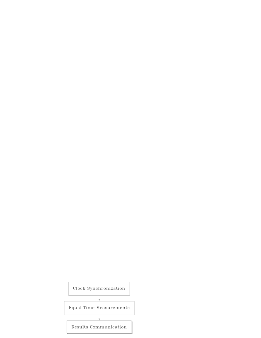
FIG. 1.: The process of local measurement in the relativistic space-time. In the first and last steps, the observers remain causally (in a classical sense) connected. The observers are separated by space-like distances in the second step when the “equal time” measurements are carried out. The correlation between these observers in the second step can only be quantum mechanical, which is known to violates classical causality manifested in the violation of Bell’s inequality.

There is no guarantee in quantum world that the refined image of the system obtained under such a procedure should be identical to that of the one obtained by doing a low resolution global measurement, in which a uniform (in space-time) external field is exerted on the system and the response of the system to the external field is measured, like the ones that determine the bulk properties of the system frequently studied in non-relativistic condensed matter system. Such a subtle difference is believed to originate from the quantum interference effects which are best illustrated by the classical double slit experiments where when one does not care which slit the microscopic particle (e.g., an electron) go, there is a interference pattern on the screen behind the double slits, but as long as one determines which slit the microscopic particle went through, the interference pattern disappears. The interference pattern can not be obtained by summing over the two pictures obtained separately by knowing exactly which slit the microscopic particle go. Such a behavior is no longer a theoretical conjecture but a experimental fact which is demonstrated recently by experiments from different groups around the world. The same difference should manifest in quantum field theory in the local versus global observables. The importance of an understanding of such a difference has not been appreciated due to the lack of a comparing theoretical frame-work. A consistent local theory for quantum field theory at finite field strength (leading to finite density of matter and energy) is constructed [1, 2] not only for understand such a difference but also for describing the problems raised in high energy physics and astrophysics.

I shall discuss one of the problems in constructing a local finite density quantum field theory for fermions in this talk, those who are interested in the original works can read the papers [1, 2]. The particular problem that I am going to to discuss here is about the necessity of including fermionic statistical block effects in the chiral symmetry breaking phase of light quark system. But before we can discuss the problem, let us first brief review what the local theory should be look like at the formal level and what is its most transparent properties.

II The Statistical Gauge Field

The non-relativistic many body theory for a system with variable particle number is based upon the Grand Canonical Ensemble (GCE) [3]. The partition function for the system in the GCE is related to its Hamiltonian $\widehat{H}$ and its particle number $\widehat{N}$ in the following way

$$Z=\lim_{\Omega\to\infty}Tre^{-\beta(\widehat{H}-\mu\widehat{N})},$$ (1)

where $\Omega$ is the volume of the system, $\beta=1/T$ with $T$ the temperature and $\mu$ is the chemical potential. The limit $\Omega\to\infty$ is the thermodynamical limit in which the equilibrium statistical mechanics describes physical many body system at equilibrium. A measurement of the ground state fermion number density in GCE which is given by

$$\overline{n} = \lim_{T\to 0}{\frac{\partial}{\partial\mu}}\left({\frac{T}{\Omega}}\ln Z\right)$$ (2)

corresponds to a global measurement since the chemical potential is independent of both space and time. Global measurements are most frequently carried out in condensed matter systems with a size smaller than or comparable to our human body (of order 1 meter) which permit us to study the system “as a whole”. The GCE is highly successful in describing these situations. Questions posed by high-energy physics, astrophysics and cosmology are somewhat different. The size of the systems compared to that of the resolution of the measuring apparatus are normally much larger, therefore one actually is capable of study either more details of the probed systems due to the reduction of the wave length of the probing system or only small fraction of the probed system due to the impossibility of covering the whole probed system by the probing system at the same time. One is in effect doing local measurements in these later situations.

Local measurements in quantum field theory are realized by exerting an external local field to the system at the space-time points interested, and, the measured quantity is deduced from the response of the system to the external field. For finite density systems, a Lorentz 4-vector local field $\mu^{\alpha}(x)$, called the primary statistical gauge field, is introduced. The ground state expectation value of fermion number density can be expressed as the functional derivative

$$\overline{\rho}(x) = {\frac{\delta\ln Z}{\delta\mu^{0}(x)}}$$ (3)

with $Z$ a functional of $\mu^{\alpha}$. It corresponds to a local measurement in the ground state at the space-time point x.

For a concrete discussion of the consequences of substituting the global chemical potential in non-relativistic many body theory for the local primary statistical gauge field, let us consider an Lagrangian of the following form

$${\cal L}^{\prime} = {\frac{1}{2}}\overline{\Psi}(i\hbox to0.0pt{/\hss}\partial+\hbox to0.0pt{/\hss}\mu O_{3}-m)\Psi+{\cal L}_{B}+{\cal L}_{\mbox{int}}$$ (4)

with $m$ the fermion mass, ${\cal L}_{B}$ the Lagrangian density of boson fields of the system and ${\cal L}_{\mbox{int}}$ the interaction between the boson and fermion fields. An 8 component “real” fermion field $\Psi$ is used for the discussion [1] with $O_{3}$ the third Pauli matrices acting on the upper and lower 4-component of $\Psi$. In most of the cases, ${\cal L}_{\mbox{int}}=-\overline{\Psi}(\Sigma(f)-m)\Psi$ with $\Sigma$ a function(al) of the boson fields represented by $f$. It is well known that the partition functional for the system can be formally written in terms of a path integration over the dynamical fields

$$Z[\mu]=\int D[f,\Psi,\overline{\Psi}]exp(i\int d^{4}x{\cal L}^{\prime})=\int D[f]exp(iS_{\mbox{eff}})$$ (5)

which is a functional of $\mu^{\alpha}$ and $\ln Z[\mu]$ is its effective action.

The fermion degrees of freedom can be integrated out first leading to an effective Euclidean action for the boson fields and the primary statistical gauge field

$$S_{\mbox{eff}}[f,\mu] = {\frac{1}{2}}\mbox{SpLn}{\frac{[i\hbox to0.0pt{/\hss}\partial+\hbox to0.0pt{/\hss}\mu O_{3}-\Sigma(f)]}{[i\hbox to0.0pt{/\hss}\partial+\hbox to0.0pt{/\hss}\mu O_{3}-m]}}+\int d^{4}x\left[{\cal L}_{B}(f)+\mu\overline{\rho}-\overline{e}\right]$$ (6)

with “Sp” the functional trace, $\overline{e}$ the average energy density of the corresponding free system of fermions ($\Sigma=0$) and $\overline{\rho}$ is the ground state expectation value of fermion number density to be discussed in the following at the “chemical potential” $\mu\equiv\sqrt{\overline{\mu}^{\alpha}\overline{\mu}_{\alpha}}$, where $\overline{\mu}^{\alpha}$ is the ground state value of $\mu^{\alpha}$ normally provided by the external conditions that fixes the density.

The first term in Eq. 6 is invariant under the $U(1)$ statistical gauge transformation $\mu_{\alpha}(x)\to\mu^{\prime}_{\alpha}(x)=\mu_{\alpha}(x)-\partial_{\alpha}\Lambda(x)$. This is because such a gauge transformation, which transforms the partition functional $Z[\mu]$ to

$$Z[\mu]\to Z^{\prime}[\mu]=Z[\mu^{\prime}]$$ (7)

can always be compensated, at least for the first term in Eq. 6 by a change of the fermionic integration variable

$$\Psi(x) \to e^{i\Lambda(x)O_{3}}\Psi(x)$$ (8)

$$\overline{\Psi}(x) \to e^{-i\Lambda(x)O_{3}}\overline{\Psi}(x)$$ (9)

so that

$$Z[\mu^{\prime}]=Z[\mu],$$ (10)

which means that fermionic quantum fluctuation contribution to $Z[\mu]$ is invariant under the gauge transformation. Such a gauge invariance is connected to the conservation of fermion number. Therefore I call the 4-vector $\mu^{\alpha}$ the statistical gauge field. Since $\mu^{\alpha}$ is a local field, its excitation represents certain collective excitations of the system. Its general dynamics in different phases of the system at low energy can be derived [1].

III The Instability of GCE in the Relativistic Space-Time

The Euclidean effective action for the boson field given by Eq. 6 can be evaluated in the usual way [1]. Since the effective action given by Eq. 6 is a canonical functional of $\mu^{\alpha}$, we can make a Legendre transformation of it, namely

$$\widetilde{S}_{\mbox{eff}}=S_{\mbox{eff}}-\int d^{4}x\overline{\mu}_{\alpha}\overline{j}^{\alpha}$$ (11)

with $\overline{j}^{\alpha}$ the ground state current of fermion number density, to make it a canonical functional of the fermion density in order to study the stability of the vacuum state against fluctuations in fermion number.

The effective potential characterizing the above mentioned energy density can be defined using $\widetilde{S}_{\mbox{eff}}$ for space-time independent background $f$ fields:

$$V_{\mbox{eff}}=-\widetilde{S}_{\mbox{eff}}/V_{4}$$ (12)

with $V_{4}$ the volume of the space-time box that contains the system. The stability of the vacuum state against the fluctuations in fermion number density around $\overline{\rho}=0$ can be studied using $V_{\mbox{eff}}$, which is a canonical function of $\overline{\rho}$. Minimization of $V_{\mbox{eff}}$ with respect to $\mu$ gives the vacuum value $\rho_{vac}$ of the system since the vacuum $\overline{\rho}$ is a monotonic function of $\mu$.

The local finite density theory can be examined by applying it to the chiral symmetry breaking phase of the half bosonized Nambu Jona-Lasinio model for the 3+1 dimension and the chiral Gross-Neveu model for 2+1 dimensions with its effective potential given by

$$V_{\mbox{eff}}=iN_{g}\int{\frac{d^{D}p}{(2\pi)^{D}}}\left[\ln\left(1-{\frac{\sigma^{2}}{p_{+}^{2}}}\right)+\ln\left(1-{\frac{\sigma^{2}}{p_{-}^{2}}}\right)\right]+{\frac{1}{4G_{0}}}\sigma^{2}+\overline{e},$$ (13)

where “$D$” is the space-time dimension, $G_{0}$ is the coupling constant and $p^{2}_{\pm}=(p_{0}\pm\mu)^{2}-\mbox{\boldmath{p}}^{2}$.

The integration over the momentum $p^{\mu}$ in Eq. 13 is divergent, a cutoff is needed to regulate the theory so that finite results can be obtained. Whatever the cutoff scheme is, one qualitative feature is true, namely, the stable minima of $V_{eff}$ move from $\sigma=0$ to $\sigma=\pm\sigma_{vac}\neq 0$ as the coupling constant $G_{0}$ is increased above a critical value $G_{0c}$.

Since the logarithmic functions in Eq. 13 has branch cuts on the real $p^{0}$ axis, the choice for the integration contour for $p^{0}$ is important. The physical $p^{0}$ integration contour is shown by $C_{Phys}$ in Fig. 2, which goes under the real axis when $p^{0}<0$ and above the real axis when $p^{0}>0$.

FIG. 2.: The set of contours belonging to the same physical class. Contour $C_{Phys}$ is the original physical contour in the Minkowski space. Contour $C_{E}$ is the Euclidean contour. Contour $C_{+}$ is the quasiparticle contour. $\pm i\pi$ denote the imaginary part of the integrand along the edges of its cuts (thick lines) on the physical $p_{0}$ plane.

It is possible to do the momentum space integration by doing the $p^{0}$ integration first without a cutoff in it, namely,

$$V_{\mbox{eff}}=iN_{g}\int{\frac{d^{D-1}p}{(2\pi)^{D-1}}}\int_{C_{Phys}}{\frac{dp^{0}}{2\pi}}\left[\ln\left(1-{\frac{\sigma^{2}}{p_{+}^{2}}}\right)+\ln\left(1-{\frac{\sigma^{2}}{p_{-}^{2}}}\right)\right]+{\frac{1}{4G_{0}}}\sigma^{2}+\overline{e}.$$ (14)

In such a case, the integration contours $C_{Phys}$, $C_{+}$ and $C_{E}$ are all equivalent in the 8-component “real” representation for the fermion fields, since the large $p_{0}$ behavior of the imaginary part of the logarithmic functions in Eq. 14 is of order $O(\mu^{2}/|p_{0}|^{2})$ on the physical complex $p_{0}$ sheet, which allows the distortion of the integration contour from $C_{Phys}$ to the Euclidean contour $C_{E}$ and to the quasiparticle contour $C_{+}$. Let us make a few comment: 1) the 8-component “real” representation for the fermion fields make it equivalent between contour $C_{Phys}$, $C_{+}$ and $C_{E}$. The usual 4-component representation does not has such a property [12] without an arbitrary subtraction. It is in this sense that the 8-component theory is not equivalent to the 4-component theory if finite density situation is considered 2) the quasiparticle contour $C_{+}$ is the most convenient contour to demonstrate that the quantum fluctuation term (the fermionic determinant) at the right hand side of Eq. 14 is a sum over the quasiparticle energies levels in the negative energy sea. The behavior of the quasi-particles is, at least in the approximation taken here, identical to that of genuine particles with a global mass despite the fact that the “mass” of the quasi-particles is related to the vacuum expectation value of a local field rather than a global constant 3) there is no instability due the fermion number fluctuation if the $p^{0}$ integration is done first since only the quasiparticle contributes. This integration contour for $p^{0}$ is implied in most of the phenomenological applications in the literature since it is intuitively acceptable. Such a “naturalness” is based on an implicit assumption, namely, the quasiparticles is the whole story.

However, there are a few problems in doing a unbounded $p^{0}$ integration first in a relativistic space-time. The most obvious one is related to the fact that a unbounded $p^{0}$ integration, which is done first, corresponds to an arbitrary choice of a equal-time hypersurface in space-time with zero thickness. This is not a covariant choice since the spatial component of the momentum $p^{\mu}$ integration has to be cutted off so that the spatial resolution of the theory is not infinitely high. Such a procedure, which is Newtonian in character based on a universal absolute time, is not considered fair in relativity since space and time can be related to each other by Lorentz transformation. The second one is connected to the observation that the quasiparticle does not saturate the local observables [1, 13] due to the existence of the transient and local quantum fluctuations of the order parameter $\sigma$. These important kind of transient and local quantum fluctuations, which does not decouple in the thermodynamical limit[13], are quenched if the momentum $p^{\mu}$ integration is carried out by doing an unbounded $p^{0}$ integration first.

The relativistic covariance can be maintained by cutting off the theory covariantly in the Euclidean space for the momentum $p^{\mu}$ by restricting the length of the Euclidean $p^{\mu}$ to be less than or equal to a cutoff $\Lambda\sim 1$ $GeV$. Such a covariance in cutoff is also adopted in lattice simulations of QCD on a symmetric lattice. The covariant cutoff of the theory allow the observers on each space-time point of the measuring hypersurface to have a resolution in time (speed of light $c=1$) of the same order as the spatial resolution. Therefore we are not talking about absolute equal-time, which does not make sense in relativity, but the kind of “equal-time” defined operationally in Fig. 1. It is not expected that the difference between these two kind of cutoff procedure can be removed by renormalization since such differences are physical that shall not be renormalized away.

It can be shown that if the covariant integration procedure is adopted, then $\partial^{2}V_{\mbox{eff}}/\partial\mu^{2}|_{\mu=0}<0$ as long as $\sigma\neq 0$ and $D\geq 2$, which implies that the $\sigma\neq 0$ state with $\overline{\rho}=0$ is not stable against fermion number fluctuations. Such a conclusion is independent of any cutoff scheme (smooth or sharp) and cutoff value for $\Lambda$. The dependence of the effective potential on the time component of the statistical gauge field is plotted in Fig. 3

FIG. 3.: The $\mu$ dependence of $V_{eff}$ of the conventional approach in the $\alpha$ phase. It has two minima at non-zero $\mu$. Here $\Lambda$ is the Euclidean momentum cutoff that defines the model.

Such a result is both theoretically and physically unacceptable since it would result in large CP violation in the strong interaction vacuum state which is not observed.

IV The statistical blocking effect

It appears that the phase in which $\sigma_{vac}\neq 0$ has a tendency to generate finite density of fermion. Such an unexpected behavior may reflect the fact that some thing is missing in our formalism used so far.

An inspection of the Folk space structure of the vacuum state in the $\sigma_{vac}\neq 0$ phase reveals the problem. It is know that in such a case, the vacuum state is condensed with finite density of fermion–antifermion pairs, namely,

$$\overline{n}_{Q\overline{Q}}=\lim_{V_{3}\to\infty}{\overline{N}_{Q\overline{Q}}\over V_{3}}\neq 0$$ (15)

with $N_{Q\overline{Q}}$ the number of the $Q\overline{Q}$ pairs and $V_{3}$ the spatial volume of the system respectively. This is because

$$\sigma_{vac}\sim\mathopen{\langle vac\,|}\overline{\psi}\psi\mathclose{|\,vac\rangle}$$ (16)

so

$$\mathclose{|\,vac\rangle}=C_{0}\mathclose{|\,0\rangle}+C_{1}\mathclose{|\,Q\overline{Q}\rangle}+C_{2}\mathclose{|\,Q\overline{Q}Q\overline{Q}\rangle}+\ldots$$ (17)

with the number of $Q\overline{Q}$ pairs proportional to $V_{3}$ if $\sigma_{vac}\neq 0$. Like the Fermi sea in the condensed matter system of fermions, these fermion–antifermion pairs can produce the statistical blocking effects inside of the system. Such statistical blocking effects can not be progressively generated by including higher order loops in a perturbative expansion of the effective action. This is because the perturbative terms correspond to a modification of the properties of the system due to finite number of fermions at any specific order of the perturbation expansion. An effect of Eq. 15 can only be accounted for by non-perturbative means. I proposed a modification of the causal structure of the theory to include the statistical blocking effect [1] in a similar way as the chemical potential do to the theory for the finite density situations. Fig. 4.b is a graphical representation of the non-perturbative sea used for our asymptotic ensemble in which the maximum filled energy level in the positive energy states is controlled by the statistical block parameter $\varepsilon$.

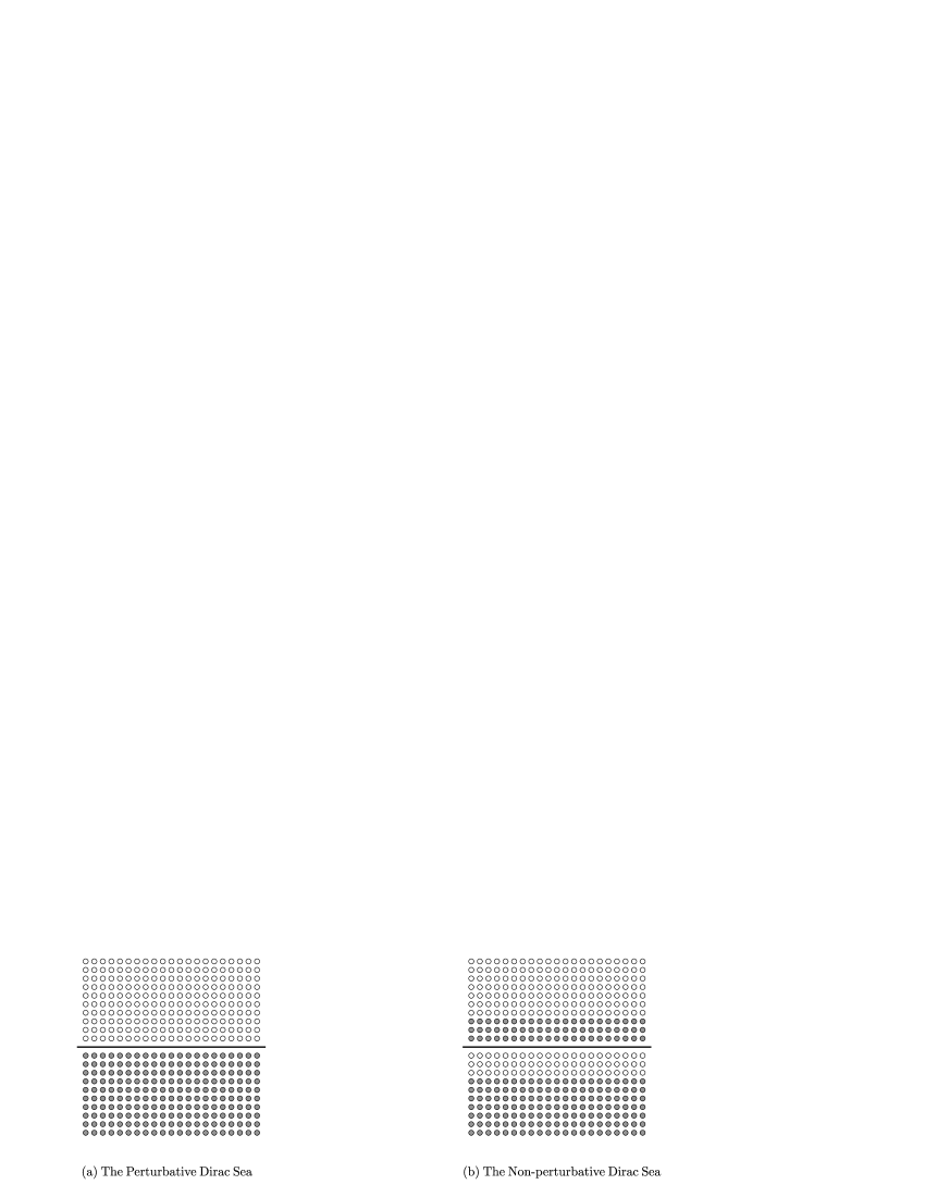
FIG. 4.: The perturbative and non-perturbative Dirac sea for the bare particles. The hollow circles represent the empty states.

It can be shown that if Fig. 4.b is chosen, the energy integration contour $C_{Phys}$ has to be distorted to ${\cal C}_{Phys}$ drawn in Fig. 5

FIG. 5.: The $p^{0}$ integration contour for the effective action for transition amplitudes between states in which both the fermion and antifermion states with absolute value of their energy below $\varepsilon$ filled. The thick lines extending to positive and negative infinity represent the branch cuts of the logarithmic function.

The effective potential $V_{eff}$ depends, in addition to other conventional ones, the statistical blocking parameter $\varepsilon$. Eq. 13 should be replaced by [1]

$$V_{\mbox{eff}}(\sigma,\mu,\varepsilon)=iN_{g}\int_{{\cal C}_{Phys}}{\frac{d^{D}p}{(2\pi)^{D}}}\left[\ln\left(1-{\frac{\sigma^{2}}{p_{+}^{2}}}\right)+\ln\left(1-{\frac{\sigma^{2}}{p_{-}^{2}}}\right)\right]+{\frac{1}{4G_{0}}}\sigma^{2}+{N_{g}\over 4\pi^{2}}\left(\mu^{4}+2\varepsilon^{4}+12\mu^{2}\varepsilon^{2}\right)$$ (18)

which should be evaluated in the Euclidean space in a way that preserves the analytic properties of Fig. 5 and cutted off covariantly.

The stability of the resulting effective potential for $D=4$ is represented in terms of equal $V_{eff}$ contour in Fig. 6 with a nonvanishing $\sigma/\Lambda=1$ and $\Lambda\sim 1$ $GeV$ is the covariant cutoff. The effective potential is not stable if both $\mu$ and $\varepsilon$ are zero. The minima at finite $\mu$ are now local minima rather than global. The global minima are located at finite $\varepsilon$ and vanish $\mu$ at which point $\partial^{2}V_{\mbox{eff}}/\partial\mu^{2}>0$ and $\partial^{2}V_{\mbox{eff}}/\partial\varepsilon^{2}>0$ which means that they are stable.

FIG. 6.: The contour plot of the equal $V_{\mbox{eff}}$ in the phase in which $D=4$, $\sigma/\Lambda=1.0$. The point $\mu=0$ and $\varepsilon=0$ is not stable both in the $\pm\varepsilon$ direction and in the $\pm\mu$ direction. The absolute minima of the effective potential is located at about $\mu=0$ and $\varepsilon/\Lambda=\pm 0.1$. There is also a pair of local minima located at $\mu/\Lambda=\pm 0.1$ and $\varepsilon=0$.

Therefore, the statistical blocking parameter cure the CP problem mentioned above. Some of the implications of having a non-vanishing $\varepsilon$ in the $\sigma_{vac}\neq 0$ phase of the vacuum is discussed in Refs. [1, 2].

V The Properties of Color Superconductivity

The ground states of the strong interaction could have different phases from the chiral symmetry breaking phase or the $\alpha$-phase [4, 5, 6, 7, 8]. They are characterized by a condensation of diquarks causing color superconductivity. Such a possibility is interesting because it may be realized in the early universe, in astronomical objects and events, in heavy ion collisions, inside nucleons [7, 9, 10] and nuclei, etc.. For the possible scalar diquark condensation in the vacuum, a half bosonized model Lagrangian is introduced [11, 1], which reads

$${\cal L}_{I} = {\frac{1}{2}}\overline{\Psi}\left[i{\hbox to0.0pt{/\hss}\partial}-\sigma-i\vec{\pi}\cdot\vec{\tau}\gamma^{5}O_{3}-\gamma^{5}{\cal A}_{c}\chi^{c}O_{(+)}-\gamma^{5}{\cal A}^{c}\overline{\chi}_{c}O_{(-)}\right]\Psi-{\frac{1}{4G_{0}}}(\sigma^{2}+\vec{\pi}^{2})+{\frac{1}{2G_{3^{\prime}}}}\overline{\chi}_{c}\chi^{c},$$ (19)

where $\sigma$, $\vec{\pi}$, $\overline{\chi}_{c}$ and $\chi^{c}$ are auxiliary fields with $(\chi^{c})^{\dagger}=-\overline{\chi}_{c}$ and $G_{0}$, $G_{3^{\prime}}$ are coupling constants of the model. ${\cal A}_{c}$ and ${\cal A}^{c}$ $(c=1,2,3)$ act on the color space of the quark; they are ${\cal A}_{c_{1}c_{2}}^{c}=-\epsilon^{cc_{1}c_{2}}$ ${\cal A}_{c,c_{1}c_{2}}=\epsilon^{cc_{1}c_{2}}$ with $\epsilon^{abc}$ ($a,b=1,2,3$) the total antisymmetric Levi–Civitá tensor. Here $O_{(\pm)}$ are raising and lowering operators respectively in the upper and lowering 4 components of $\Psi$.

This model has two non-trivial phases. The vacuum expectation of $\sigma$ is non-vanishing with vanishing $\chi^{2}\equiv-\overline{\chi}_{c}\chi^{c}$ in the $\alpha$-phase. The vacuum state in the $\alpha$-phase is condensed with quark-antiquark pairs. The vacuum expectation of $\sigma$ is zero with finite $\chi^{2}$ that spontaneously breaks the $U(1)$ statistical gauge symmetry in the second phase, which is called the $\omega$-phase. There is a condensation of correlated scalar diquarks and antidiquarks in the color $\overline{3}$ and $3$ states in the $\omega$-phase of the vacuum state.

Since diquarks and antidiquarks are condensed in the $\omega$-phase, it is expected that an exchange of the role of $\varepsilon$ and $\mu$ occurs. It is found to be indeed true: there are also two sets of minima for the effective potential, the first set is the one with finite $\mu=\pm\mu_{vac}$ and $\varepsilon=0$ and the second set corresponds to $\mu=0$ and finite $\varepsilon=\pm\varepsilon_{vac}$ in the $\omega$-phase of the model. But here the absolute minima of the system in the $\omega$-phase correspond to the first set of solutions, in which the CP invariance and baryon number conservation are spontaneously violated due to the presence of a finite vacuum $\mu^{\alpha}_{vac}$. The stability of the resulting effective potential is represented in Figs. 7 and 8

FIG. 7.: The contour plot of the equal $V_{\mbox{eff}}$ in the phase in which $\chi_{vac}/\Lambda=1.0$. The point $\mu=0$ and $\varepsilon=0$ is also not stable both in the $\pm\varepsilon$ direction and in the $\pm\mu$ direction. The local minima of the effective potential is located at about $\mu=0$ and $\varepsilon/\Lambda=\pm 0.15$. There is also a pair of absolute minima located at $\mu/\Lambda=\pm 0.3$ and $\varepsilon=0$.

FIG. 8.: The 3D plot of $V_{\mbox{eff}}$ in the phase in which $\chi_{vac}/\Lambda=1.0$.

This conclusion is also applicable to the $\beta$-phase of $p$-wave diquark condensation models [4, 5] with vector fermion pair and antifermion pair condensation, in which the chiral symmetry $SU(2)_{L}\times SU(2)_{R}$ is also spontaneously broken down. It is shown in Fig. 9 and 10

FIG. 9.: The contour plot of the equal $V_{\mbox{eff}}$ in the phase in which $\sqrt{\phi^{2}_{vac}}/\Lambda=1.0$. The point $\mu=0$ and $\varepsilon=0$ is also not stable both in the $\pm\varepsilon$ direction and in the $\pm\mu$ direction. The local minima of the effective potential is located at about $\mu=0$ and $\varepsilon/\Lambda=\pm 0.15$. There is also a pair of absolute minima located at $\mu/\Lambda=\pm 0.3$ and $\varepsilon=0$.

FIG. 10.: The 3D plot of $V_{\mbox{eff}}$ in the phase in which $\sqrt{\phi^{2}_{vac}}/\Lambda=1.0$.

Therefore, the statistical blocking parameter $\varepsilon$ and the primary statistical gauge field $\mu^{\alpha}$ provide a more complete set of macroscopic parameters to describe the condensation of fermionic particles in a relativistic system. Their physical meaning is also clear. The statistical gauge field characterizes the condensation of particle (pairs), which has net fermion number. The color superconducting phase is caused by condensation of fermion pairs, which implies that fermion pairing or antifermion pairing are favored against the fermion–antifermion pairing. The matter antimatter tends to separate in the color superconducting phase resulting in genesis of matter. The statistical blocking parameter characterizes the concentration of fermion–antifermion pairs with no net fermion number. The chiral symmetry breaking phase, on the other hand, favors the fermion–antifermion pairing. It is not surprising that $\varepsilon\neq 0$ in the chiral symmetry breaking phase.

VI Summary

In summary, it is important to take into account, among others ones discussed in Refs. [1, 2], of the statistical blocking effect in a localized finite density theory.

REFERENCES

- [1] S. Ying, Ann. Phys. 266, 295 (1998).
- [2] S. Ying, Report No. hep-th/9908087; S. Ying, Commun. Theor. Phys. Accepted.
- [3] See, e.g., K. Huang K Statistical Mechanics (Willy, New York, 1963).
- [4] S. Ying, Phys. Lett. B283, 341 (1992).
- [5] S. Ying, 1996 Ann. Phys. (NY) 250, 69 (1996).
- [6] T. Schäfer, Phys. Rev. D57, 950 (1998).
- [7] M. Alford, K. Rajagopal, and F. Wilczek, Phys. Lett. B422, 247 (1998).
- [8] R. Rapp, T. Schäfer, E. V. Shuryak, and M. Velkovsky, Phys. Rev. Lett. 81, 53 (1998).
- [9] S. Ying, J. Phys. G22, 293 (1996); S. Ying, Commun. Theor. Phys. 28, 301 (1997).
- [10] S. Ying, Report No. hep-ph/9912519.
- [11] S. Ying, Report No. hep-ph/9604255.
- [12] S. Ying, Report No. hep-th/9611166.
- [13] S. Ying, Report No. hep-ph/9704216.