Spinodal Instabilities and the Dark Energy Problem

Abstract

The accelerated expansion of the Universe measured by high redshift Type Ia Supernovae observations is explained using the non-equilibrium dynamics of naturally soft boson fields. Spinodal instabilities inevitably present in such systems yield a very attractive mechanism for arriving at the required equation of state at late times, while satisfying all the known constraints on models of quintessence.

One of the most startling developments in observational cosmology is the mounting evidence for the acceleration of the expansion rate of the Universe[1]. Coupled with cluster abundance and CMB observations, these data can be interpreted as evidence for a cosmological constant $\Lambda$ which contributes an amount $\Omega_{\Lambda}\simeq 0.7$ to the critical energy density while matter contributes $\Omega_{\text{matter}}\simeq 0.3$, leading to a flat FRW cosmology (see [2] and references therein).

While introducing a cosmological constant may be a cosmologically sound explanation of the observations, it is a worrisome thing to do indeed from the particle physics point of view. It is hard enough to try to explain a vanishing cosmological constant, given the various contributions from quantum zero point energies, as well as from the classical theory[3], but at least one could envisage either a symmetry argument (such as supersymmetry, if it were unbroken) or a dynamical approach (such as the ill-fated wormhole approach[4]) that could do the job. It is much more difficult to see how cancellations between all possible contributions would give rise to a non-zero remnant of order $10^{-47}$ GeV⁴ which is extremely small compared to $M_{\text{Planck}}^{4}$ or $M_{\text{SUSY}}^{4}$, the “natural” values expected in a theory with gravity or one with a supersymmetry breaking scale $M_{\text{SUSY}}$. Even from the cosmological perspective, a cosmological constant begs the question of why its effects are dominating now, as opposed to any time prior to today, especially given its different redshifting properties compared to matter or radiation energy density.

These fine tuning problems can at least be partially alleviated if instead of using a ${\em constant}$ energy density to drive the accelerated expansion, a dynamically varying one were used instead. This is the idea behind Quintessence models[5]. A scalar field whose equation of state violated the strong energy condition (i.e. with $\rho+3P<0$ ) during its evolution[6] would serve just as well as a cosmological constant in terms of explaining the data, as long as its equation of state satisfied the various known constraints for such theories [7]. However, an arbitrary scalar field whose energy density dominates the expansion rate is not sufficient to get out of all fine tuning problems; in particular, for a field of sufficiently small mass that it would only start evolving towards its minimum relatively recently (i.e. masses of order the inverse Hubble radius), the ratio of matter energy density $\rho_{m}$ to field energy density $\rho_{\phi}$ would be need to be incredibly fine tuned at early times so as to have $\rho_{m}/\rho_{\phi}\sim 1$ today. The quintessence approach uses so-called tracker fields[8] that have potentials that drive the field to attractor configurations that have a a fixed value of $\rho_{m}/\rho_{\phi}$. Thus, for these models, regardless of the initial conditions, the intermediate time value of $\rho_{m}/\rho_{\phi}$ will always be the same. The only fine tuning required in these models is the timing of the deviation of $\rho_{\phi}$ from the tracking solutions to allow it to satisfy the condition $\rho_{\phi}+3P_{\phi}<0$ today.

What we propose is a working alternative to the idea of tracker fields without the usual fine tuning problems. Recent work on the non-equilibrium dynamics of quantum fields[9, 10] has shown that under certain circumstances the back reaction of quantum fluctuations can have a great influence on the evolution of the quantum expectation value of a field [11, 12], to the extent that using the classical equations of motion can grossly misrepresent the actual dynamics of the system. What we will show below is that we can make use of this modified dynamical behavior to construct models that might allow for a more natural setting for a late time cosmological constant.

The class of models we consider are those using pseudo-Nambu-Goldstone bosons (PNGBs) to construct theories with naturally light scalars[13]. Such models have been used for late time phase transitions[14], as well as to give rise to a cosmological “constant” that eventually relaxed to zero[15], not unlike what we want to do here. However, our take on these models will be significantly different from that of ref.[15].

We can write the required energy density as $\rho_{\text{Dark Energy}}\sim\left(10^{-3}\text{ eV}\right)^{4}$, which is suggestive of a light neutrino mass scale[16, 17]. There is a way to construct models of scalar fields coupled to neutrinos where the scalar field potential naturally (in the technical sense of t’Hooft[18]) incorporates the small mass scale $m_{\nu}^{4}$.

Consider a Lagrangian containing a Yukawa coupling of the form[13]:

$$-{\cal L}_{\text{Yuk}}=\sum_{j=0}^{N-1}\left(m_{0}+\varepsilon\exp i\left(\frac{\Phi}{f}+\frac{2\pi j}{N}\right)\right)\overline{\nu}_{jL}\nu_{jR}+\text{h.c.}$$ (1)

The scale $f$ is the scale at which a the global symmetry that gives rise to the Nambu-Goldstone mode $\Phi$ is spontaneously broken. The Lagrangian ${\cal L}_{\text{Yuk}}$ is to be thought of as part of the low-energy effective theory of $\Phi$ coupled to neutrinos at energies below $f$.

The term proportional to $\varepsilon$ could be obtained by a coupling to a Higgs field $\chi$ that acquires an expectation value $\left\langle\chi\right\rangle=f/\sqrt{2}\exp i\frac{\Phi}{f}$. Note that in the absence of $m_{0}$ this Yukawa term possesses a continuous chiral $U\left(1\right)$ symmetry. The term proportional to $m_{0}$ breaks this symmetry explicitly to a residual discrete $Z_{N}$ symmetry given by:

$$\nu_{j}\rightarrow\nu_{j+1},\text{ }\nu_{N-1}\rightarrow\nu_{0},\text{ }\Phi\rightarrow\Phi+\frac{2\pi f}{N}.$$ (2)

This interaction can generate an effective potential for the Nambu-Goldstone mode $\Phi$ which must vanish in the limit that $m_{0}\rightarrow 0$ which is equivalent to the vanishing of the neutrino masses. Since $\Phi$ is an angular degree of freedom, it should not be a surprise that the effective potential is periodic and of the form

$$V\left(\Phi\right)=M^{4}\left(1+\cos\frac{N\Phi}{f}\right).$$ (3)

Here $M$ should be associated with a light neutrino mass $m_{\nu}\sim 10^{-3}$ eV.

Here, we have followed the working hypothesis of [15] which states that the effective vacuum energy will be dominated by the heaviest fields still evolving towards their true minimum. We assume that the super light PGNB field $\Phi$, with associated mass of order $\sim m_{\nu}^{2}/f$, will be the last field still rolling down its potential. Thus we have chosen by hand the constant in eq.(3) so that when $\Phi$ reaches the minimum it will have zero cosmological constant associated with it. This choice is essentially a choice of the zero of energy at asymptotically late times.

The finite temperature behavior associated with these models is extremely interesting[19]. For $N\geq 3$ the $\Phi$ dependent part of the potential can be written as

$$c\left(T\right)M^{4}\cos\frac{N\Phi}{f},$$ (4)

where $c\left(T\right)$ vanishes at high temperature $T$. Thus the high temperature phase of the theory has a non-linearly realized $U\left(1\right)$ symmetry where the $\Phi$ potential becomes exactly flat with value $M^{4}$. Since $M\sim m_{\nu}$ this cosmological constant contribution will have no effect during nucleosynthesis and through the matter dominated phase until $T\sim M$. At this time $c\left(T\right)$ reaches its asymptotic value of unity and we have the potential in eq.(3). For $N=2$, $c\left(T\right)$ changes sign continously, passing through zero at the critical temperature such that the high temperature minima become the low temperature maxima and vice-versa. There is a $Z_{2}$ symmetry in both the low and high temperature phases.

The potential in eq.(3) has regions of spinodal instability, i.e. where the effective mass squared is negative. These occur when $\cos N\Phi/f>0.$ If $\Phi$ is in this region, modes of sufficiently small comoving wavenumber follow an equation of motion that at least for early times is that of an inverted harmonic oscillator. This instability will then drive the non-perturbative growth of quantum fluctuations until they reach the spinodal line where $\cos N\Phi/f=0$[12]. Since the quantum fluctuations grow non-pertrubatively large, we have to resum perturbation theory to regain sensible behavior and this is done by the Hartree truncation [12]. The prescription is to first expand $\Phi$ around its (time dependent) expectation value $\left\langle\Phi\left(\vec{x},t\right)\right\rangle\equiv\phi\left(t\right)$ as

$$\Phi\left(\vec{x},t\right)=\phi\left(t\right)+\psi\left(\vec{x},t\right),$$ (5)

where the tadpole condition $\left\langle\psi\left(\vec{x},t\right)\right\rangle=0$ gives the equation of motion for $\phi\left(t\right)$. The Hartree approximation involves inserting eq.(5) into eq.(3), expanding the cosines and sines, and then making the following replacements[12]:

$$\cos\frac{N\psi}{f}\longmapsto\left(1-\frac{N^{2}\left(\psi^{2}-\left\langle\psi^{2}\right\rangle\right)}{2f^{2}}\right)\exp-\frac{N^{2}\left\langle\psi^{2}\right\rangle}{2f^{2}},\quad\sin\frac{N\psi}{f}\longmapsto\frac{N\psi}{f}\exp-\frac{N^{2}\left\langle\psi^{2}\right\rangle}{2f^{2}}.$$ (6)

The equations for the field $\phi,$ and the fluctuation modes $f_{k}$ coupled to the scale factor $a\left(t\right)$ are

$$\ddot{\phi}+3\frac{\dot{a}}{a}\dot{\phi}-\frac{NM^{4}}{f}\exp-\frac{N^{2}\left\langle\psi^{2}\right\rangle}{2f^{2}}\sin\frac{N\phi}{f}=0,$$ (7)

$$\ddot{f}_{k}+3\frac{\dot{a}}{a}\dot{f}_{k}+\left(\frac{k^{2}}{a^{2}}-\frac{N^{2}M^{4}}{f^{2}}\exp-\frac{N^{2}\left\langle\psi^{2}\right\rangle}{2f^{2}}\cos\frac{N\phi}{f}\right)f_{k}=0,$$ (8)

with

$$\left\langle\psi^{2}\right\rangle=\int\frac{d^{3}k}{\left(2\pi\right)^{3}}\left|f_{k}\right|^{2}.$$ (9)

The effective Friedmann equation for the scale factor is obtained by use of semiclassical gravity, i.e. by using $\left\langle T_{\mu\nu}\right\rangle$ to source the Einstein equations:

$$\frac{\dot{a}^{2}}{a^{2}}=\frac{8\pi}{3M_{p}^{2}}\left[\rho_{m}(t)+\frac{1}{2}\dot{\phi}^{2}+\frac{1}{2}\langle\dot{\psi}^{2}\rangle+\frac{1}{2a^{2}}\left\langle(\vec{\nabla}\psi)^{2}\right\rangle+M^{4}\left(1+\cos(N\phi/f)\exp-\frac{N^{2}\left\langle\psi^{2}\right\rangle}{2f^{2}}\right)\right],$$ (10)

with

$$\rho_{m}(t)=\rho_{m}(t_{i})\frac{a^{3}(t_{i})}{a^{3}(t)}$$ (11)

being the matter density and $t_{i}$ being the time at which the PGNB field begins its evolution.

The interesting feature of the above equations of motion is the appearance of terms involving $\exp-\frac{N^{2}\left\langle\psi^{2}\right\rangle}{2f^{2}}$. These multiply terms in the potential and its various derivatives that contain the non-trivial $\phi$ dependence. What we expect to have happen is that as the spinodally unstable modes grow, they will force $\left\langle\psi^{2}\right\rangle$ to grow as well. This in turn will rapidly drive the exponential terms to zero, leaving a term proportional to $M^{4}$ in the Friedmann equations, which will act as a cosmological constant at late times.

If we consider the $N\geq 3$ models, then at temperatures larger than $T_{\text{crit}}\sim M$ the potential is just given by $M^{4}$ and is swamped by both the matter and radiation contributions to the energy density. Since the potential is flat, we expect that the zero mode is equally likely to attain any value between $0$ and $2\pi$ and in particular, we expect a probability of order $\sim 1/2$ for the initial value to lie above the spinodal line. If there was an inflationary period before this phase transition, we expect that the zero mode will take on the same value throughout the region that will become the observable universe today.

As the temperature decreases, the non-trivial parts of the potential turn on and the zero mode begins its evolution towards the minimum once the Universe is old enough, i.e. $H\left(T_{\text{roll}}\right)\sim m_{\phi}\sim M^{2}/f$. At the same time, if the zero mode started above the spinodal line, the fluctuations begin their spinodal growth. Whether the spinodal instabilities have any cosmological effect depends crucially on a comparison of time scales, the first being between the time $t_{\ast}$ it takes the zero mode to reach the spinodal point at $\phi_{\text{spinodal}}/f=\pi/2N$ under the purely classical evolution (i.e. neglecting the fluctuations), and the time $t_{\text{spinodal}}$ it takes for the fluctuations to sample the minima of the tree-level potential, so that $N^{2}\langle\psi^{2}\rangle/f^{2}\sim{\cal O}\left(1\right)$. Since the growth of instabilities will stop at times later than $t_{\ast}$, if spinodal instabilities are to be at all relevant to the evolution of $\phi$, we need $t_{\text{spinodal}}\ll t_{\ast}$. By looking at the equations of motion we can argue that[11]

$$t_{\text{spinodal}}\simeq\frac{f}{2M^{2}}\ln\frac{f^{2}}{N^{2}\langle\psi^{2}\rangle\left(t_{i}\right)}+\frac{3}{2H_{i}},$$ (12)

where $t_{i}$ is the time at which the zero mode starts to roll and $H_{i}$ is the Hubble parameter at this time. Furthermore the early time behavior of the equations of motion gives us

$$t_{\ast}\simeq\frac{f}{M^{2}}\ln\frac{f}{N\phi(t_{i})}+\frac{3}{2H_{i}}.$$ (13)

Comparing eqs.(12,13), we see that to have the spinodal instabilities be significant we need $\phi^{2}(t_{i})\ll\langle\psi^{2}\rangle\left(t_{i}\right)$.

The other condition that needs to be met is that there should be sufficient time for the spinodal instabilities to dominate the zero mode evolution before today. This will ensure that the expansion of the Universe will be driven by the remnant cosmological constant $M^{4}$ at the times relevant to the SNIa observations. For large enough initial fluctuations we can make the spinodal time as early as we need.

What sets the scale of the initial fluctuations? If we assume a previous inflationary phase, we can treat the PGNB as a minimally coupled massless field and the standard inflationary results should apply[20]. The initial conditions for the mode functions are then given by:

$$f_{k}\left(t_{i}\right)=\frac{i}{\sqrt{2k^{3}}}H_{DS}\ \text{\ for }\kappa\leq k\leq H_{i},$$ (14)

where $\kappa$ is an infrared cutoff corresponding to horizon size during the De Sitter phase and $H_{DS}$ is the Hubble parameter during inflation. The short wavelength modes ($k>H_{i}$) have their conformal vacuum initial conditions. With these initial conditions

$$\frac{\langle\psi^{2}\rangle\left(t_{i}\right)}{f^{2}}\simeq\frac{H_{DS}^{2}}{4\pi^{2}f^{2}}\left(N_{\text{e-folds}}-60\right).$$ (15)

and for $H_{DS}\simeq 10^{13}$ GeV, $N_{\text{e-folds}}-60\simeq 10^{5}$, and $f\simeq 10^{15}$ GeV, we would only need that $\phi(t_{i})/f\ll 0.5$. These are not outlandish parameter values and we see that very little fine tuning is required. In fact, there is a great deal of freedom in choosing the values of these parameters, the only requirement being that the ratio of parameters appearing in (15) not be so small that the required value of $\phi(t_{i})/f$ is overly restricted.

In the figures below we use these parameters as well as $M\simeq 5.5\times 10^{-3}$ eV corresponding to neutrino masses, beginning the evolution at a redshift $1+z=1200$. In Fig. 1 we plot the numerical evolution of the zero mode and of the growth of the fluctuations, while Fig. 2 shows the equation of state of the PNGB field and the total equation of state including PNGB and matter components as a function of redshift. What we quickly infer from these graphs is that the evolution of the Universe becomes dominated by the remnant cosmological term, leading to an evolution toward a late time equation of state $w\equiv P/\rho\simeq-1$. The equation of state today is seen to be $w\simeq-0.7$ and indicates a matter component $\Omega_{\text{matter}}=0.3$ and a cosmological constant-like component $\Omega_{\text{pngb}}=0.7$. Because the PNGB component has an equation of state $w=-1$ by a redshift as high as $z=50$, these results reproduce the best fit spatially flat cosmology of the SNIa data[1].

One feature of this model is that the parameter $M$ is directly related to the measured value of today’s Hubble constant. We find

$$M=\left(5.5\times 10^{-3}\text{eV}\right)\left(\frac{H_{0}}{65\frac{\text{km}}{\text{s{\hbox{\cdot}}Mpc}}}\right)^{1/2}\left(\frac{\Omega_{\text{pngb}}}{0.7}\right)^{1/4}\;,$$ (16)

which is to be compared to the observed $90\%$ confidence range of $\Delta m^{2}$ from the Super Kamiokande contained events analysis[16] of $5\times 10^{-4}\text{eV}^{2}<\Delta m^{2}<6\times 10^{-3}\text{eV}^{2}$, and the more recent results of the up-down asymmetry analysis[17] which indicates a range $1.5\times 10^{-3}\text{eV}^{2}<\Delta m^{2}<1.5\times 10^{-2}\text{eV}^{2}$, whereas the small and large mixing angle MSW solutions of the solar neutrino problem[21, 22] yield a range of $5\times 10^{-6}\text{eV}^{2}<\Delta m^{2}<4\times 10^{-4}\text{eV}^{2}$.

There is no shortage of models to explain the accelerating expansion of the universe. However, most options are lacking in motivation and require significant fine tuning of initial conditions or the introduction of a fine tuned small scale into the fundamental Lagrangian. We too have a fine tuned scale: the neutrino mass. However, we can take solace in the fact that this fine tuning is related to a particle that can be found in the Particle Data Book[23], with known mechanisms to produce the required value, and experiments dedicated to its measurement.

The model itself is also relatively benign, not requiring invocations of String or M-theory to justify its potential. Chiral symmetry breaking leading to PNGB’s is not unheard of in nature (pions do exist after all!), and should probably be expected in GUT or SUSY symmetry breaking phase transitions involving coupled scalars. This, together with the dynamical effects of backreaction allow the present model to be successful in explaining the data with only minor tuning of initial conditions.

Acknowledgement 1

D.C. was supported by a Humboldt Fellowship while R.H. was supported in part by the Department of Energy Contract DE-FG02-91-ER40682.

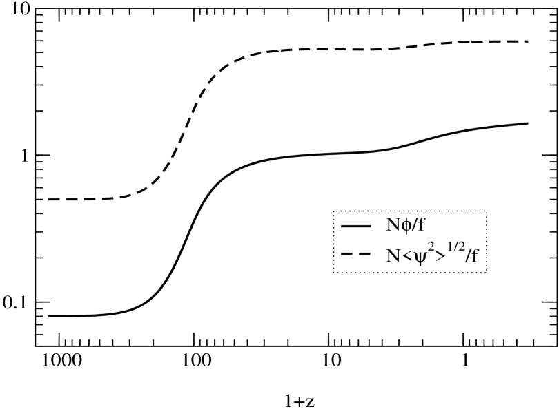
FIG. 1.: The evolution of the zero mode $\phi$ and the root mean square flucutation $\langle\psi^{2}\rangle^{1/2}$ as a function of the redshift $1+z$ from recombination at $1+z\simeq 1200$ to today at $1+z=1$ and beyond. The parameters used for the simulation correspond to $M=5.5\times 10^{-3}$ eV, $f/N=10^{15}$ GeV and $(N_{\text{e-folds}}-60)H_{\text{DS}}^{2}=10^{31}(\text{GeV})^{2}$. For convenience we have used $(N_{\text{e-folds}}-60)=10$, which is necessary to avoid numerical implementation of an infrared cutoff of order $\exp(-10^{5})$. This has the effect of slightly underestimating $\langle\psi^{2}\rangle$ as the evolution proceeds compared to the case of $(N_{\text{e-folds}}-60)=10^{5}$, but will not change any qualitative features of the evolution. The initial conditions are $N\phi(t_{i})/f=0.08$ and $\dot{\phi}(t_{i})=0$.

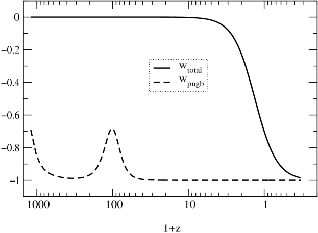
FIG. 2.: The total equation of state $w_{\text{total}}=P_{\text{pngb}}/(\rho_{\text{matter}}+\rho_{\text{pngb}})$ and the PNGB equation of state $w_{\text{pngb}}=P_{\text{pngb}}/\rho_{\text{pngb}}$ as a function of redshift. The parameters were chosen as in Fig. 1.

REFERENCES

- [1] S.J. Perlmutter et al., Nature 391, 51 (1998); S.J. Perlmutter et al., astro-ph/9812133 (1998); A.G. Riess et al., Astron. J. 116, 1009 (1998).
- [2] N.A. Bahcall, J.P. Ostriker. S. Perlmutter and P.J. Steinhardt, Science 284, 1481 (1999).
- [3] S. Weinberg, Rev. Mod. Phys. 61, 1, (1989).
- [4] S. Coleman, Nucl. Phys. B310 643 (1988).
- [5] R.R. Caldwell, R.Dave and P.J. Steinhardt, Phys. Rev. Lett. 80, 1582 (1998); I. Zlatev, L. Wang and P.J. Steinhardt, Phys. Rev. Lett 82 896 (1999); related works are: T.Barreiro, E. J. Copeland and N.J. Nunes, astro-ph/9910214 (1999); Andreas Albrecht and Constantinos Skordis, astro-ph/9908085 (1999); Varun Sahni and Limin Wang, astro-ph/9910097 (1999).
- [6] N. Weiss, Phys. Rev. Lett. 42 197 (1987); C. Wetterich, Astron. and Astrophy. 301, 321 (1995); B. Ratra and P.J.E. Peebles, Phys. Rev. D37 3406 (1988); P. Ferreira and M. G. Joyce, Phys. Rev. Lett. 79, 4740 (1997); Phys. Rev. D58, 023503 (1998).
- [7] L. Wang, R.R. Caldwell, J.P. Ostriker and P.J. Steinhardt, astro-ph/9901388 (1999).
- [8] P.J. Steinhardt, L. Wang and I. Zlatev, Phys. Rev. D59, 123504 (1999).
- [9] J. Schwinger, J. Math. Phys. 2, 407 (1961); P.M. Bakshi and K.T. Mahanthappa, J. Math. Phys. 4, 1 (1963); ibid, 12; L.V. Keldysh, Sov. Phys. JETP 20, 1018 (1965).
- [10] D. Cormier, Non-Equilibrium Field Theory Dynamics in Inflationary Cosmology, hep-ph/9804449 (1998), and references therein.
- [11] D. Boyanovsky, D. Cormier, H.J. de Vega, R. Holman, A. Singh and M. Srednicki, Phys. Rev. D56, 1939 (1997).
- [12] D. Cormier and R. Holman, Phys. Rev. D60, 41301 (1999); hep-ph/9912483 (1999).
- [13] C.T. Hill and G.G. Ross, Nucl. Phys. B311, 253 (1988); Phys. Lett. 203B, 125 (1988).
- [14] C.T. Hill, D.N. Schramm and J. Fry, Comm. Nucl. Part. Phys. 19, 25 (1989); I. Wassermann, Phys. Rev. Lett. 57, 2234 (1986); W. H. Press, B. Ryden and D. Spergel, Ap. J. 347, 590 (1989).
- [15] J.A. Frieman, C.T. Hill, A. Stebbins and I. Waga, Phys. Rev. Lett. 75, 2077 (1995); see also K. Coble, S. Dodelson, and J. Frieman, Phys. Rev. D 55, 1851 (1997).
- [16] Y. Fukuda et al., Phys. Rev. Lett. 81, 1562 (1998).
- [17] Y. Fukuda et al., Phys. Lett. B467, 185 (1999).
- [18] G. ’t Hooft in Recent Developments in Gauge Theories, eds. G. ’t Hooft, et al (Plenum Press, New York and London, 1979), p. 135.
- [19] Arun K. Gupta, C. T. Hill, R. Holman and E.W. Kolb, Phys. Rev. D45, 441 (1992).
- [20] A. Linde, Particle Physics and Inflationary Cosmology, (Harwood Academic Publishers, Switzerland, 1990).
- [21] L. Wolfenstein, Phys. Rev. D17, 2369 (1978); S.P. Mikheyev and A.Yu. Smirnov, Sov. Jour. Nucl. Phys. 42, 913 (1985).
- [22] J.N. Bahcall, P.I. Krastev and A.Yu. Smirnov, Phys. Rev. D58, 096016 (1998).
- [23] C. Caso et al., Eur. Phys. J. C3, 1 (1998).