SLAC-PUB-8319 SU-ITP-99/53 January, 2000

TeV Strings and Collider Probes of Large Extra Dimensions

Schuyler Cullen

Department of Physics
Stanford University, Stanford, California 94305 USA

Maxim Perelstein and Michael E. Peskin

Stanford Linear Accelerator Center
Stanford University, Stanford, California 94309 USA

ABSTRACT

Arkani-Hamed, Dimopoulos, and Dvali have proposed that the fundamental gravitational scale is close to 1 TeV, and that the observed weakness of gravity at long distances is explained by the presence of large extra compact dimensions. If this scenario is realized in a string theory of quantum gravity, the string excited states of Standard Model particles will also have TeV masses. These states will be visible to experiment and in fact provide the first signatures of the presence of a low quantum gravity scale. Their presence also affects the more familiar signatures due to real and virtual graviton emission. We study the effects of these states in a simple string model.

Submitted to Physical Review D

1 Introduction

Traditionally, the weakness of gravitational interactions at the scales accessible to particle physics experiments has been explained by postulating that the Planck scale at which gravity becomes strong is very high, $M_{\mbox{\scriptsize Pl}}\sim 10^{19}$ GeV. Below this scale, ordinary quantum field theory applies, but, when this scale is reached, one can observe the underlying quantum theory that incorporates quantum gravity. A disappointing feature of the traditional framework is that the enormously high value of the Planck scale prevents us from observing any effects of quantum gravity in laboratory experiments in the conceivable future, which means that the search for the quantum theory of gravity has to proceed without any experimental input. Recently Arkani-Hamed, Dimopoulos, and Dvali (ADD) [1] have proposed an alternative to this pessimistic scenario. They have constructed models in which gravity becomes strong at a scale $M$ of order 1 TeV. They explain the apparent weakness of gravity at lower energies by the presence of compact dimensions with compactification radius $R\gg M^{-1}$. We will call these ‘large extra dimensions’. In this framework, gravity could have significant effects on particle interactions at the energies accessible to current experiments and observations [2].

So far, almost all work on the phenomenological implications of large extra dimensions has concentrated on the effects of real and virtual graviton emission. It is the basic assumption of the model that gravitons can move in the extra dimensions. Then the graviton quantum states will be characterized by a (quantized) momentum in the extra dimensions. The states with nonzero momentum are called Kaluza-Klein (KK) excitations; they can be described equivalently as massive spin-2 particles in 4 dimensions, with mass equal to the higher-dimensional momentum, which couple to Standard Model particles through a coupling to the energy-momentum tensor $T^{\mu\nu}$ with strength $M_{\mbox{\scriptsize Pl}}^{-1}$. The sum over these states leads gravity to become strong at a scale $M\ll M_{\mbox{\scriptsize Pl}}$ because the spectrum of KK excitations becomes exceedingly dense as the size $R$ of the compact dimensions is taken to be much larger than $M^{-1}$.

Because the low-energy coupling of the KK excitations is model-independent, one can study processes in which gravitons are emitted into the extra dimensions [3, 4, 5] in the context of a low-energy effective field theory. For collision energies much less than $M$, the cross sections for missing-energy signatures are not sensitive to the details of physics at the scale $M$. This fact allows one to obtain model-independent bounds on $M$. On the other hand, it means that the simple observation of graviton emission does not give information about the nature of the fundamental gravity theory.

The approach of low-energy effective field theory can also be applied to processes in which the KK excitations appear as virtual exchanges contributing to the scattering of Standard Model particles [3, 6, 7]. In this case, the contribution of low-energy effective field theory is cutoff-dependent and of the same order as that from possible higher-dimension operators. In phenomenological analyses, the virtual KK exchange is typically represented as a dimension-8 contact interaction of the form $T^{\mu\nu}T_{\mu\nu}$ with a coefficient proportional to $1/M^{4}$. The precise value of this coefficient depends on the underlying model. It is also possible that this model could predict additional contact interactions with a different spin structure that could also be observed as corrections to Standard Model scattering processes. For these reasons, the virtual exchanges cannot be used to put lower bounds on $M$. On the other hand, the presence of high-spin contact interactions can produce impressive signals, and the measurement of the coefficients of these interactions can give new information on the fundamental theory.

The study of large extra dimensions differs from other phenomenological problems in that the underlying theory from which the low-energy effective description is derived is a theory of quantum gravity. This fact may bring in new and unforseen consequences. In particular, the only known framework that allows a self-consistent description of quantum gravity is string theory [8]. But string theory is not simply a theory of quantum gravity. As an essential part of its structure, not only the gravitons but also the particles of the Standard Model must have an extended structure. This means that, in a string theory description, there will be additional modifications of Standard Model amplitudes due to string excitations which might compete with or even overwhelm the modifications due to graviton exchange.

In this paper, we will study the signatures of string theory in a simple toy model with large extra dimensions. The most important effects in this model come from the exchange of string Regge (SR) excitations of Standard Model particles. We will show that, in Standard Model scattering processes, contact interactions due to SR exchange produce their own characteristic effects in differential cross sections. We will also show that these typically dominate the effects due to KK exchange. In addition, the SR excitations can be directly produced as resonances. These effects have been discussed previously, but at a more qualitative level, by Lykken [10], and by Tye and collaborators [11]. The effects of SR resonances have also been studied some time ago, in the context of composite models of quarks and leptons, by Bars and Hinchliffe [12].

The dominance of SR over KK effects is a generic feature of weakly-coupled string theory. It follows from the counting of coupling constants in string perturbation theory [9], which is illustrated in Figure 1. To model the ADD scenario, we consider open string theories which contain at low energy a set of Yang-Mills gauge bosons that can be identified with gauge bosons of the Standard Model. We denote the dimensionless Yang-Mills coupling by $g$. Figure 1(a) shows the string generalization of a Standard Model two-body scattering amplitude at order $g^{2}$. This amplitude coincides with the Standard Model expectation in the limit in which the center-of-mass energy is much lower than the string scale $M_{S}$ and, at higher energy, shows corrections proportional to powers of $(s/M_{S}^{2})$. These are the effects of SR excitations. Figure 1(b) shows the leading string contribution to graviton emission. The graviton is a closed string state, and thus this process involves the closed-string coupling constant, which is of order $g^{2}$; the full amplitude is of order $g^{3}$. Figure 1(c) shows one contribution to the one-loop corrections to two-body scattering. This diagram is of order $g^{4}$. However, as Lovelace [13] originally showed, this string diagram contains the graviton-exchange contribution when factorized as indicated in the figure. Thus, the exchange of gravitons and their KK excitations are suppressed with respect to SR exchange by a factor $g^{2}$ in the amplitude.

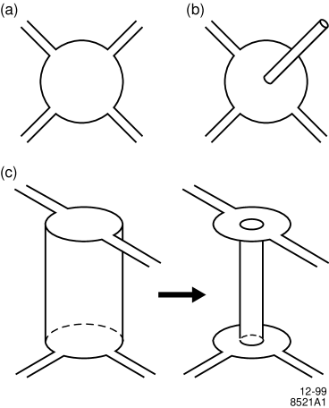
Figure 1: Schematic diagrams contributing to scattering amplitudes in a string generalization of the Standard Model: (a) tree-level 2-body scattering; (b) graviton emission; (c) loop-level 2-body scattering.

In this paper, we will flesh out the picture represented by Figure 1 using an illustrative toy string model. In Section 2, we will present this model, which uses scattering amplitudes on the 3-brane of weakly-coupled Type IIB string theory to describe a string version of Quantum Electrodynamics with electrons and photons. In Section 3, we will apply this model to compute the cross sections for Bhabha scattering and $e^{+}e^{-}\to\gamma\gamma$ at high energy. In Section 4, we will discuss the phenomenological consequences of those results, both for contact interactions in high-energy scattering and for the direct observability of SR resonances. We will find a direct bound on the string scale of $M_{S}>1$ TeV. Translated into a bound on the fundamental quantum gravity scale, this becomes $M>1.6$ TeV. This bound is admittedly model-dependent, but it is also larger than any other current limit by more than a factor of two for the relevant case of 6 large extra dimensions.

In the remainder of the paper, we will discuss the more familiar signatures of large extra dimensions in string language. In Section 5, we will study the KK graviton emission process $e^{+}e^{-}\to\gamma G$. In Section 6, we will discuss the effects of virtual KK graviton exchange through a detailed analysis of the process of $\gamma\gamma$ elastic scattering. This analysis will also allow us to derive the relation between the string scale and the fundamental quantum gravity scale. In Section 7, we will review the collider limits on large extra dimensions in the light of the new picture presented in this paper. Section 8 will present our conclusions. A series of appendices review formulae for the analysis of Bhabha scattering and present some of the more technical details of the string calculations.

A number of the topics considered in Sections 5 and 6 have recently been considered, from a slightly different point of view, in a paper of Dudas and Mourad [14]. The phenomenological importance of SR resonances in models with a low string scale has been discussed briefly by Accomando, Antoniadis, and Benakli [15].

2 The model

In this paper, we would like to investigate the simplest model that illustrates the influence of string Regge (SR) excitations on physical cross sections. Thus, we will be content to study a simple embedding of the Quantum Electrodynamics of electrons and photons into string theory. This theory contains only one gauge group and only vectorlike couplings. More realistic string models with large extra dimensions have been constructed by Kakuzhadze, Tye, and Shiu [16], Antoniadis, Bachas, and Dudas [17], and Ibanez, Rabadan, and Uranga [18]. These models are quite complicated. The added structure is inessential to the general phenomenological picture that we will present in this paper, though there are many model-dependent details that would be interesting to study.

With this motivation, we consider a very simple embedding of QED into Type IIB string theory. In this theory, there exists a stable BPS object, the D3-brane, which is a 4-dimensional hypersurface on which open strings may end. We will assume that the 10-dimensional space of the theory has 6 dimensions compactified on a torus with a periodicity $2\pi R$, and that $N$ coincident D3-branes are stretched out in the 4 extended dimensions. The massless states associated with open strings that end on the branes are described by an $N=4$ supersymmetric Yang-Mills theory with a gauge group $U(N)$. These states include gauge bosons $A^{\mu a}$, gauginos $\widetilde{g}^{ai}$, and complex scalars $\phi^{a}$, where $a$ is an index of the adjoint representation of $U(N)$ and $i$ runs from 1 to 4. We will project this theory down to a $U(1)$ gauge theory with two massless Weyl fermions and identify the gauge boson and fermions of that theory with the photon and electron of QED.

We take the parameters of this theory to be the string scale $M_{S}={{\alpha^{\prime}}}^{-1/2}$ and the (dimensionless) Yang-Mills coupling constant $g$, which we identify with a Standard Model gauge coupling. (Except for this definition of $g$, we adopt the conventions of [9]). Note that $M_{S}$ is directly observable: The SR resonances occur at masses $M_{n}=\sqrt{n}M_{S}$, for $n=1,2,\ldots$.

The gravitational constant and other physical scales in the theory are derivable from $M_{S}$ and $g$. However, the relation involves one-loop calculations and is model-dependent, depending on the full spectrum of the theory. Quite generally in the ADD scenario, the Newton constant which represents the observed strength of gravity is given in terms of the fundamental gravitational scale $M$ by the relation [2, 3, 4, 19]

$$(4\pi G_{N})^{-1}=M^{n+2}R^{n}\ ,$$ (1)

where the compact dimensions are taken to be flat and periodic with period $2\pi R$. Our toy model corresponds to the case $n=6$. In Section 6 we will present a simple but model-dependent computation of the relation between $M$ and string scale $M_{S}$. We will show that

$${M\over M_{S}}=\left({1\over\pi}\right)^{1/8}\alpha^{-1/4}\ ,$$ (2)

where $\alpha=g^{2}/4\pi$. Then, for two extreme choices,

$$\alpha=1/137 \to M/M_{S}=3.0\ ;$$

$$\alpha=\alpha_{s}(\mbox{1\ TeV}) \to M/M_{S}=1.6\ .$$ (3)

In scattering amplitudes involving virtual gravitons, the gravity scale will enter as $M^{-4}$, and so the string and gravity effects will be well-separated in size. For future reference, the tension of the D3-brane is given by [9]

$$\tau_{3}={1\over 8\pi^{3}}\alpha^{-1}M_{S}^{4}\ .$$ (4)

The relations in (3) illustrate the most problematical aspect of our analysis. The naive string constructions we will use in this paper require all of the Standard Model gauge couplings to be unified at the string scale. Proposals for splitting these couplings to realistic values using the vacuum expectation value of a string modulus field are given in [17, 18]. However, in this paper we will deal with the Standard Model interactions only one at a time.

The explicit embedding that we will use is the following: Consider the $SU(2)$ subgroup of $U(N)$ with generators

$$t^{+}={1\over\sqrt{2}}\pmatrix{0&1\cr 0&0\cr}\ ,\qquad t^{-}={1\over\sqrt{2}}\pmatrix{0&0\cr 1&0\cr}\ ,\qquad t^{3}={1\over 2}\pmatrix{1&0\cr 0&-1\cr}\ .$$ (5)

(In general, we normalize $SU(N)$ generators to ${\mbox{\rm tr}}[t^{a}(t^{b})^{\dagger}]=\frac{1}{2}\delta^{ab}$.) We can identify the left-handed electron $e^{-}_{L}$, the left-handed positron $e^{+}_{L}$, and the photon $A_{\mu}$ as

$$e^{-}_{L}=\widetilde{g}^{-1}\ ,\qquad e^{+}_{L}=\widetilde{g}^{+1}\ ,\qquad A_{\mu}=A_{\mu}^{3}\ ,$$ (6)

where the superscript denotes the matrix from (5) which would be used in computing the Chan-Paton factor. The three generators form a closed operator algebra, and in fact the tree amplitudes of $N=4$ super-Yang-Mills theory which have only these states on external lines also involve only these states on internal lines. In string theory, we can reduce the massless sector to this set of states by an appropriate orbifold projection [20]. (For example, in a $U(2)$ theory, mod out by $Z_{2}\times Z_{3}$, where $Z_{2}$ is the center of $SU(2)$ and the internal indices $i$ are assigned the $Z_{3}$ phases $1,\zeta,\zeta,\zeta$, with $\zeta=e^{2\pi i/3}$). This gives an explicit prescription for computing tree-level string corrections to QED amplitudes. The electric charge of the electron is given by

$$e=g\ ,$$ (7)

as one can determine from the commutator $[t^{+},t^{3}]$. To compute loop corrections, we should properly extend this theory to a full modular-invariant string construction. Instead, for simplicity, we will use the content of the original $N=4$ supersymmetric theory to compute the loop diagram studied in Section 6.

Most of our analysis will be carried out at the tree level in string theory. A tree-level amplitude for a particular process actually depends only on whether that process involves open- or closed-string states and is otherwise independent of which weak coupling string theory it belongs to. Beyond this, it depends only on the correlation function of the vertex operators associated with the external particles for that process and is independent of the remainder of the string spectrum. If the tree amplitude for a process involves four particles from an $N=4$ supersymmetric string theory, the amplitude is identical whether the full theory has $N=4$ supersymmetry or is nonsupersymmetric. This identity is explicit when a nonsupersymmetric model is constructed as an orbifold of a supersymmetric theory and, in that situation, is a special case of the ‘inheritance’ property of orbifolds. This identity is also familiar in field theory, where tree-level scattering amplitudes in QCD are computed by recognizing that they are identical to amplitudes in a supersymmetric generalization of QCD [21]. Thus, the string corrections to tree-level Standard Model amplitudes that we will compute in this paper are actually valid for any situation in which the quarks and leptons come from the untwisted sector of an open string orbifold.

Our tree amplitudes are model-independent in another way. An alternative string construction of the ADD scenario would be to consider Type IIA string theory with 5 dimensions large and one dimension small. Then the ADD scenario would arise if the Standard Model particles were bound to a D4-brane wrapped around the small dimension. Similarly, one could consider $n$ large and $(6-n)$ small dimensions, with a D$(9-n)$-brane wrapped around the small dimensions. If the small dimensions are smaller than 1/TeV, all external states would necessarily carry zero momentum in these directions. Then actually the tree amplitudes derived in this paper would apply for any value of $n$. We should also note that while we assume the toroidal compactification of the extra dimensions here, we expect the results for scattering of open strings on the D brane in Sections 3 and 4 to remain valid for models with a warp factor in the bulk [22], provided that the bulk curvature is sufficiently small near the brane.

3 Stringy corrections to $e^{+}e^{-}\to\gamma\gamma$ and Bhabha scattering

In this section, we will use our toy model to compute the effects of TeV scale strings on Bhabha scattering and $\gamma\gamma$ production in $e^{+}e^{-}$ collisions. We will compute the leading-order scattering amplitudes in string theory, using the external states described in the previous section.

Tree amplitudes of open-string theory are given as sums of ordered amplitudes multiplied by group theory Chan-Paton factors [9]. We consider amplitudes with all momenta directed inward. Let the ordered amplitude with external states $(1,2,3,4)$ be denoted $g^{2}A(1,2,3,4)$. Then the full scattering amplitude ${\cal A}(1,2,3,4)$ is given by

$${\cal A}(1,2,3,4) = g^{2}A(1,2,3,4)\cdot{\mbox{\rm tr}}[t^{1}t^{2}t^{3}t^{4}+t^{4}t^{3}t^{2}t^{1}]$$ (8)

$$+\ g^{2}A(1,3,2,4)\cdot{\mbox{\rm tr}}[t^{1}t^{3}t^{2}t^{4}+t^{4}t^{2}t^{3}t^{1}]$$

$$+\ g^{2}A(1,2,4,3)\cdot{\mbox{\rm tr}}[t^{1}t^{2}t^{4}t^{3}+t^{3}t^{4}t^{2}t^{1}]\ .$$

To compute QED amplitudes with fixed external states, we would substitute for each $t^{i}$ the appropriate matrix from (5) (or, for outgoing states, the Hermitian conjugate matrix).

The field theory tree amplitudes of Yang-Mills theory can be cast into the same form [21], and it is useful to consider that case first. Only a subset of the possible 4-point ordered amplitudes are nonzero; those amplitudes are given in Figure 2. In this figure, a wavy external line denotes a gauge boson, and a straight external line denotes a fermion. The sign denotes the helicity (for states directed inward). The diagrams are presented with the $s$-channel vertical and the $t$-channel horizontal. Actually, the four amplitudes involving fermions can be derived from the two with only gauge bosons by the use of $N=1$ supersymmetry Ward identities, and these identities also imply the vanishing of the ordered amplitudes for helicity combinations not shown in the figure. The two 4-gauge boson amplitudes are related by $N=2$ supersymmetry. This is an example of the model-independence discussed at the end of the previous section.

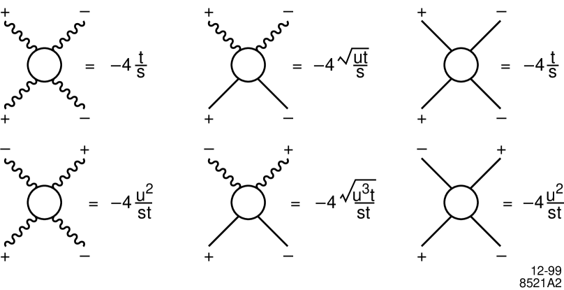
Figure 2: Nonzero 4-point ordered tree amplitudes of Yang-Mills theory. Wavy lines represent gauge bosons; straight lines represent fermions. The sign for each line is the helicity, directed inward.

It is straightforward to check that these formulae give the familiar QED tree amplitudes. For example, for $e^{-}_{L}e^{+}_{R}$ elastic scattering, only the first line of (8) has a nonzero Chan-Paton factor and we find

$${\cal A}(e^{-}_{L}e^{+}_{R}\to e^{-}_{L}e^{+}_{R})=-2e^{2}{u^{2}\over st}=2e^{2}u\left({1\over s}+{1\over t}\right)\ ,$$ (9)

with $g=e$. For $e^{+}e^{-}$ annihilation to $\gamma\gamma$, all three terms contribute and we find, for example,

$${\cal A}(e^{-}_{L}e^{+}_{R}\to\gamma_{L}\gamma_{R})=-e^{2}\sqrt{{u\over t}}\left[{u\over s}+{t\over s}-1\right]=2e^{2}\sqrt{{u\over t}}\ .$$ (10)

The generalization of the formulae in Figure 2 to string states on a D-brane is known to be quite simple [23, 24] : All of the amplitudes shown in the figure are multiplied by the common factor

$${\cal S}(s,t)={\Gamma(1-{\alpha^{\prime}}s)\Gamma(1-{\alpha^{\prime}}t)\over\Gamma(1-{\alpha^{\prime}}s-{\alpha^{\prime}}t)}\ .$$ (11)

This factor is essentially the original Veneziano amplitude [25]. Before we apply this result, it will be useful to sketch its derivation.

In the model described in Section 2, the electron and photon states are massless states of open strings ending on the D3-brane. These states are described by the quantum theory of fluctuations of an open string in which the string fields have Neumann boundary conditions in the $\mu=$ 0–3 directions and Dirichlet boundary conditions in the $\mu=$ 5–10 directions. The string world surface has the topology of a disk, as shown in Figure 3(a). The scattering amplitudes are evaluated by mapping this surface onto a circle in the complex plane, as in Figure 3(b), and then into the upper half plane. External open string states are represented by operators, called ‘vertex operators’, placed on the boundary, and group theory matrices $t^{a}$, the Chan-Paton factors. When the boundary is mapped to the real line, the vertex operators appear in a given order 1,2,3,4, and their correlation function gives the ordered amplitude $A(1,2,3,4)$ which appears in (8). By summing over all orderings, one builds up the complete formula for ${\cal A}(1,2,3,4)$.

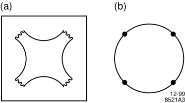
Figure 3: Schematic illustration and world-sheet diagram of the scattering process involving four open strings on a D-brane.

The explicit formula for the 4-point ordered amplitude is [9, 26]

$$A(1,2,3,4)={1\over{\alpha^{\prime}}^{2}}X^{2}\int_{0}^{1}dx\left<\prod_{i=1}^{4}{\cal V}_{q_{i}}(x_{i},k_{i})\right>\ ,$$ (12)

where ${\cal V}_{q_{i}}(x_{i})$ is the vertex operator of the state $i$. The operators are placed on the real axis at $x_{i}=0,x,1,X$, with $X$ to be fixed and sent to $\infty$. The index $q_{i}$ denotes the superconformal charge, which for the disk amplitude is constrained by $\sum_{i}q_{i}=-2$.

A good way to account for the boundary conditions on the real line is to perform the ‘doubling trick’, which represents left-moving fields on the world-sheet by fields in the upper half plane and right-moving fields by their continuation to the lower half plane. Explicitly, let us split the worldsheet boson field into its holomorphic and antiholomorphic parts:

$$X^{\mu}(z,\overline{z})=X^{\mu}(z)+\overline{X}^{\mu}(\overline{z}).$$ (13)

The boundary conditions imposed on $X(z)$ and the worldsheet fermion field $\psi(z)$ on the real line are then

$$X^{\mu}(z)=\pm\overline{X}^{\mu}(\overline{z}),\,\,\,\,\psi^{\mu}(z)=\pm\overline{\psi}^{\mu}(\overline{z}),$$ (14)

where the plus sign corresponds to $\mu=0-3$ (Neumann boundary conditions), and the minus sign to $\mu=5-10$ (Dirichlet boundary conditions.) The fields $X(z)$ and $\psi(z)$ are originally defined only on the upper half-plane, $\cal{C}^{+}$. We extend the definitions of these fields to the full plane by identifying

$$X^{\mu}(z)=\pm\overline{X}^{\mu}(z)\ ,\qquad\psi^{\mu}(z)=\pm\overline{\psi}^{\mu}(z)\ ,\qquad z\in{\cal C}^{-},$$ (15)

where the plus and minus signs again correspond to the Neumann and Dirichlet boundary conditions. With these definitions, the correlation functions of these fields are given by

$$\left<X^{\mu}(w)X^{\nu}(z)\right> = -{{\alpha^{\prime}}\over 2}g^{\mu\nu}\ln|w-z|,$$

$$\left<\psi^{\mu}(w)\psi^{\nu}(z)\right> = g^{\mu\nu}(w-z)^{-1},$$ (16)

for any $\mu$ and $\nu$.

The open string vertex operators are built from the worldsheet boson and fermion fields $X^{\mu}$ and $\psi^{\mu}$, the spin field $\Theta_{\alpha}$, and the superconformal ghost field $\phi$. We work in the space-time metric $(-,+,\ldots,+)$, and define the conventional Mandelstam variables by $s=-2k_{1}\cdot k_{2}$, $t=-2k_{1}\cdot k_{4}$, and $u=-2k_{1}\cdot k_{3}$. Then, for photons, the vertex operators with $q=-1$ and $q=0$ take the form

$${\cal V}_{-1}^{\mu}(x,k) = (2{{\alpha^{\prime}}})^{1/2}e^{-\phi}\psi^{\mu}e^{i2k\cdot X}(x),$$

$${\cal V}_{0}^{\mu}(x,k) = 2(i\partial X^{\mu}+{\alpha^{\prime}}k\cdot\psi\psi^{\mu})e^{i2k\cdot X}(x)\ .$$ (17)

These expressions are referred to, respectively, as the ‘$-1$ picture’ and the ‘0 picture’. The factor of 2 in the exponentials compensates for the replacement of the full $X^{\mu}(z,\overline{z})$ by its holomorphic part in (13). For fermions, the vertex operator with with $q=-1/2$ (‘$-1/2$ picture’) is

$${\cal V}_{-1/2}^{\alpha}(x,k)=2^{1/2}{{\alpha^{\prime}}}^{3/4}e^{-\phi/2}\Theta^{\alpha}e^{i2k\cdot X}(x).$$ (18)

Note that for open strings, the momenta and polarization tensors are required to be parallel to the D-brane, so all the fields that appear in the vertex operators (17) and (18) have Neumann boundary conditions. It is then not surprising that the result (11) is identical to the corresponding result in type I string theory.

The correlators required for the calculation are given by (16) and

$$\left<e^{-\phi(w)}e^{-\phi(z)}\right> = (w-z)^{-1},$$

$$\left<\Theta_{\alpha}(w)\Theta_{\beta}(z)\right> = C_{\alpha\beta}(w-z)^{-5/4},$$ (19)

where $C_{\alpha\beta}$ is the charge conjugation matrix. Explicitly evaluating the expressions (12) with these vertex operators and correlators, one finds the expressions in Figure 2 multiplied by the form factor (11), as promised.

A check on the normalization of the 0 picture operator is given by the operator product relation

$$\epsilon_{2}\cdot{\cal V}_{-1}(x,k_{2})\,\,\epsilon_{1}\cdot{\cal V}_{0}(0,k_{1}) \sim$$ (20)

$$\hskip-133.69994pt-{\alpha^{\prime}}x^{2k_{1}\cdot k_{2}{\alpha^{\prime}}-1}\left\{\epsilon_{1}\cdot\epsilon_{2}(k_{1}-k_{2})_{\mu}+2\epsilon_{1}\cdot k_{2}\epsilon_{2\mu}-2\epsilon_{2}\cdot k_{1}\epsilon_{1\mu}\right\}{\cal V}_{-1}^{\mu}(0,k_{1}+k_{2})+\Delta\ ,$$

where $\Delta$ is a total derivative in $x$. A similar relation holds for ${\cal V}_{0}(x,k_{2}){\cal V}_{0}(0,k_{1})$. When inserted into (8), these relations give the correct factorization to a pole in $(k_{1}+k_{2})^{2}$ and the three-gluon vertex, as shown in Figure 4. The relative normalization of ${\cal V}_{0}$ and ${\cal V}_{-1}$ is given by the picture-changing relation [9]. Then comparison of the four-point amplitudes to those of Yang-Mills theory gives the normalization of (12).

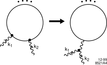
Figure 4: Factorization of the open-string amplitude to produce a pole in $(k_{1}+k_{2})^{2}$ and a three-gluon vertex.

To compare string amplitudes to Standard Model amplitudes, we are typically interested in the limit in which $s$, $t$, $u$ are much less than the string scale $M_{S}={\alpha^{\prime}}^{-1/2}$. In this limit,

$${\cal S}(s,t)=\left(1-{\pi^{2}\over 6}{st\over M_{S}^{4}}+\cdots\right)\ .$$ (21)

It is interesting that, in the toy model, the leading corrections are proportional to $M_{S}^{-4}$, corresponding to an operator of dimension 8. This is a consequence of the fact that the first higher-dimension operator with $N=4$ supersymmetry appears at dimension 8 [27]. It is likely that in more general string models in which quarks and leptons appear from twisted sectors of the orbifold, the first string corrections would be proportional to $M_{S}^{-2}$.

Now we can apply the form factor (11) to representative QED processes. For Bhabha scattering, only the first Chan-Paton factor is nonzero, and so we find

$${\cal A}(e^{-}_{L}e^{+}_{R}\to e^{-}_{L}e^{+}_{R}) = -2e^{2}{u^{2}\over st}{\cal S}(s,t)\ ,$$

$${\cal A}(e^{-}_{L}e^{+}_{R}\to e^{-}_{R}e^{+}_{L}) = -2e^{2}{t\over s}{\cal S}(s,t)\ ,$$

$${\cal A}(e^{-}_{L}e^{+}_{L}\to e^{-}_{L}e^{+}_{L}) = -2e^{2}{s\over t}{\cal S}(s,t)\ ,$$ (22)

and the same results for the parity-reflected processes. In general, all helicity amplitudes for Bhabha scattering are given by their field theory expressions multiplied by ${\cal S}(s,t)$. This form factor has SR poles in the $s$- and $t$-channels. A $u$-channel pole cannot appear, because the open string contains no states with electric charge $\pm 2$.

For $e^{+}e^{-}\to\gamma\gamma$, the result is more complex. The string form factor appears in all three possible channels, and we find

$${\cal A}(e^{-}_{L}e^{+}_{R}\to\gamma_{L}\gamma_{R})=e^{2}\sqrt{{u\over t}}\left[{u\over s}{\cal S}(s,t)+{t\over s}{\cal S}(s,u)-{\cal S}(t,u)\right]\ .$$ (23)

The other nonzero helicity amplitudes are derived from this one by parity reflection and crossing. In particular, the amplitude for production of $\gamma_{R}\gamma_{R}$ remains zero. The amplitude (23) contains massive SR poles in all three channels.

4 String phenomenology at colliders

The expressions for stringy corrections that we have derived allow one to search for signals of string theory in collider experiments. In this section, we will discuss these explicit signatures of string theory. We begin by considering effects visible as contact interactions well below the string scale. We will then discuss direct observation of the string Regge excitations.

4.1 Contact interactions

Both two-photon production and Bhabha scattering have been studied at LEP 2 at the highest available energies. We consider first the case of two-photon production. Deviations from the Standard Model cross section have been analyzed by the LEP experiments in terms of Drell’s parametrization [28]

$${d\sigma\over d\cos\theta}={d\sigma\over d\cos\theta}\biggr{|}_{SM}\cdot\left(1\pm{2ut\over\Lambda_{\pm}^{4}}\right)\ .$$ (24)

For the case of $e^{+}e^{-}\to\gamma\gamma$, it is actually a general result that the first correction due to a higher-dimension operator comes from a unique dimension-8 operator. This operator is proportional to the cross term in $T^{\mu\nu}T_{\mu\nu}$, where $T^{\mu\nu}$ is the energy-momentum tensor of QED. Thus, Drell’s parametrization (24) should apply to any model of new physics at short distances.

To compare our string theory results to this expression, insert (21) into (23); this gives

$${\cal A}(e^{-}_{L}e^{+}_{R}\to\gamma_{L}\gamma_{R})=-2e^{2}\sqrt{{u\over t}}\left[1+{\pi^{2}\over 12}{ut\over M_{S}^{4}}+\cdots\right]\ .$$ (25)

Squaring this expression, and noting that the correction is invariant to crossing $t\leftrightarrow u$, we can identify

$$\Lambda_{+}=\left(12/\pi^{2}\right)^{1/4}M_{S}\ .$$ (26)

The OPAL collaboration [29] has reported a limit $\Lambda_{+}>304$ GeV from measurements at 183 and 189 GeV in the center of mass. The ALEPH, DELPHI, and L3 collaborations have reported similar constraints [30, 31, 32]. The OPAL result corresponds to a limit

$$M_{S}>290\ \mbox{GeV}\ ,\ \mbox{95\% conf.}$$ (27)

If we use the first line of (3) to convert this to a limit on the fundamental quantum gravity scale, we find $M>870$ GeV.

The comparison of string predictions to the data on Bhabha scattering brings in two new considerations. The first of these is that Bhabha scattering at energies above the $Z^{0}$ resonance includes $Z^{0}$ exchange as an important contribution, while the $Z^{0}$ was not a part of our string QED. To find a prescription for including both $\gamma$ and $Z^{0}$ exchange, we recall that all QED Bhabha scattering amplitudes are multiplied by the common form factor ${\cal S}(s,t)$. Thus, we suggest comparing the data on Bhabha scattering to the simple formula

$${d\sigma\over d\cos\theta}(e^{-}e^{+}\to e^{-}e^{+})={d\sigma\over d\cos\theta}\biggr{|}_{SM}\cdot\left|{\cal S}(s,t)\right|^{2}\ .$$ (28)

This is essentially the assumption that the SR excitations of the photon and the $Z^{0}$ have the same spectrum, up to contributions of size $m_{Z}^{2}$ that we can ignore in computing their masses, and that the SR excitations of the $Z^{0}$ have the same polarization asymmetry as the $Z^{0}$ in their coupling to electrons.

The second complication for Bhabha scattering is that, unlike the case of $e^{+}e^{-}\to\gamma\gamma$, there are many possible forms for the higher-dimension corrections to the Standard Model result. Already at dimension 6 there are three possible helicity-conserving operators, of which two are also parity-conserving. At dimension 8 there are 4 parity-conserving operators. Various combinations of these operators have been proposed as the basis for fits to Bhabha scattering data. It would be useful to review the most important models proposed previously and to compare them to (28).

For many years, Bhabha scattering has been of interest as the most sensitive probe of lepton substructure. The form proposed for deviations from the Standard Model prediction was the most general combination of helicity-conserving dimension-6 operators [33]

$$\delta{\cal L}={4\pi\over 2\Lambda^{2}}\left[\eta_{LL}\overline{e}_{L}\gamma^{\mu}e_{L}\overline{e}_{L}\gamma_{\mu}e_{L}+\eta_{RR}\overline{e}_{R}\gamma^{\mu}e_{R}\overline{e}_{R}\gamma_{\mu}e_{R}+2\eta_{RL}\overline{e}_{R}\gamma^{\mu}e_{R}\overline{e}_{L}\gamma_{\mu}e_{L}\right]\ ,$$ (29)

where the $\eta_{a}$ are $\pm 1$ or 0 and the mass scale $\Lambda$ is taken to be the scale of compositeness.

With the recent interest in large extra dimensions and low-scale quantum gravity, Bhabha scattering has been reconsidered as a place to look for the effects of virtual KK graviton exchange. As we have remarked in the introduction, the effect of KK exchange is not reliably computable in low-energy effective field theory. Typically, this effect is modeled by introducting an appropriate contact interaction with an adjustible coefficient [3, 6, 7]. In this paper we will follow Hewett’s convention by representing the effective Lagrangian for KK exchange as [6]:

$$\delta{\cal L}=i{4\lambda\over M_{H}^{4}}T^{\mu\nu}T_{\mu\nu}\ ,$$ (30)

where $\lambda=\pm 1$ and $T^{\mu\nu}$ is the full energy-momentum tensor of the model. Hewett writes the scale in this Lagrangian as $M_{S}$; we use the notation $M_{H}$ to distinguish this mass scale from the string scale [34].

It should be noted that the expressions (29) and (30) do not contain any powers of a small coupling constant. When these expressions are added to the Standard Model formulae, the higher-dimension operators compete with amplitudes that are of order $g^{2}$. This allows one to obtain very stringent bounds on the coefficient of the new operators. Bounds on the $\Lambda$ parameters, for example, are typically a factor of 20 higher than the center-of-mass energy of the $e^{+}e^{-}$ collisions being analyzed. The physical meaning of these bounds, however, depends on the relation between the coefficients in (29) and (30) and the predictions of the underlying fundamental theory. In Section 6, we will derive (30) from our toy string model and show that the coefficient is of order

$${1\over M_{H}^{4}}\sim{g^{4}\over M_{S}^{4}}\ .$$ (31)

Thus, (30) is parametrically suppressed with respect to the effects of SR exchange. This conclusion is generic when quantum gravity is represented by a weakly-coupled string theory, though perhaps in other models of quantum gravity (30) might be the dominant effect.

With this in mind, we will compare the models discussed above to an illustrative data set for Bhabha scattering at LEP 2. A complete analysis of the LEP 2 data is beyond the scope of this paper. For reference, we have listed the various expressions for the Bhabha scattering cross sections in these models in Appendix A.

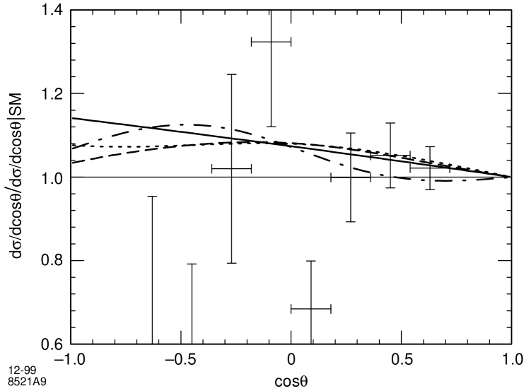
Figure 5: Comparison of data on Bhabha scattering at 183 GeV with models of corrections to the Standard Model from higher-dimension operators. The plot shows the fractional deviation from the Standard Model, $(d\sigma/d\cos\theta/d\sigma/d\cos\theta/|_{\mbox{\scriptsize SM}}-1)$ versus $\cos\theta$. The four curves represent: solid, string model with $M_{S}=410$ GeV; dotted, KK exchange with $M_{H}=830$ GeV; dashed, VV contact interactions with $\Lambda=8800$ GeV; dot-dash, AA contact interactions with $\Lambda=6700$ GeV.

The four LEP experiments have all announced preliminary results on the Bhabha scattering cross section at high energies [32, 35, 36, 37, 38] and have used the results to put limits on 4-fermion contact interactions. In particular, the L3 experiment has published their data at 183 GeV in a form convenient for our analysis. In Figure 5, we compare this data to the formula (28) and to the analogous formulae derived from (29) and (30). The curves shown are the 95% confidence exclusion limits for the various models considered: for SR exchange, $M_{S}>410$ GeV, for KK exchange with $\lambda=+1$, $M_{H}>830$ GeV, for compositeness with VV contact interactions ($\eta_{LL}=\eta_{RR}=\eta_{RL}=-1$) $\Lambda>8800$ GeV, for compositeness with AA contact interactions, ($\eta_{LL}=\eta_{RR}=-\eta_{RL}=+1$), $\Lambda>6700$ GeV. In a weakly-coupled string theory, the dominant effect would come from $M_{S}$. Using the relation (3), the exclusion limit on $M_{S}$ derived from this data would correspond to a limit on the quantum gravity scale of $M>1.2$ TeV.

A similar analysis can be used to estimate the sensitivity of experiments at future, higher-energy $e^{+}e^{-}$ colliders. As a guide, consider a linear $e^{+}e^{-}$ collider running at a center of mass energy of 1 TeV. With a 100 fb^-1 data sample, the measurement of Bhabha scattering should be systematics limited. We consider a set of 8 measurements of the differential cross sections corresponding to the bin centers in Figure 5 and assume that each measurement is made to 3% accuracy and agrees with the Standard Model expectation. Then the 95% confidence exclusion limits for the four models just considered are: for SR exchange, $M_{S}>3.1$ TeV, for KK exchange with $\lambda=+1$, $M_{H}>6.2$ TeV, for compositeness with VV contact interactions $\Lambda>88$ TeV, for compositeness with AA contact interactions, $\Lambda>62$ TeV. The corresponding deviations from the Standard Model expectation are graphed as a function of $\cos\theta$ in Figure 6. Using (3), the limit on $M_{S}$ would translate to a limit $M>9.3$ TeV on the quantum gravity scale.

A remarkable feature of Figure 6 is that the four curves shown have very different shapes. If a deviation from the Standard Model is seen, then with higher statistics or higher energy it should be possible to determine which of these theories, if any, gives the correct description.

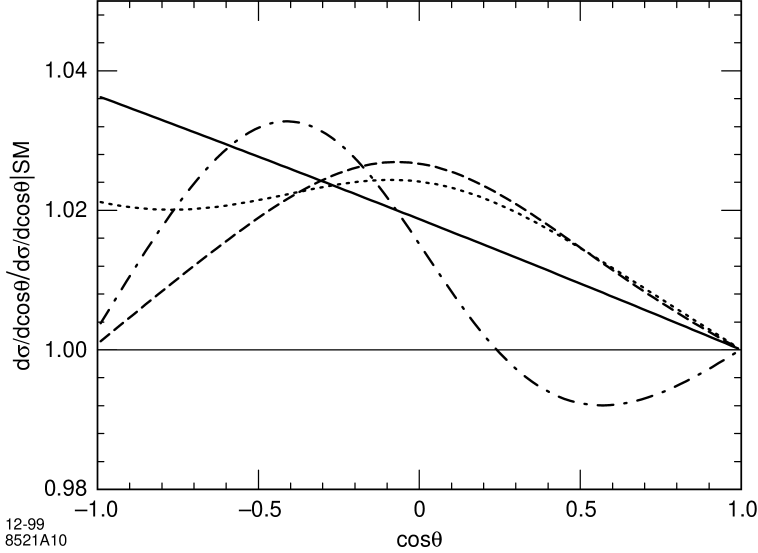
Figure 6: Comparison of deviations from the Standard Model prediction for Bhabha scattering at 1 TeV due to corrections from higher-dimension operators. The four curves represent: solid, string model with $M_{S}=3.1$ TeV; dotted, KK exchange with $M_{H}=6.2$ TeV; dashed, VV contact interactions with $\Lambda=88$ TeV; dot-dash, AA contact interactions with $\Lambda=62$ TeV.

4.2 Resonances

Though theories based on contact interactions are limited to the first deviations from the Standard Model, our string theory formulae are valid at higher energies, and we can examine their characteristic features there. The most obvious property apparent in (11) is the presence of a sequence of $s$-channel poles at masses $M_{n}=\sqrt{n}M_{S}$, for $n=1,2,\ldots$. It is interesting to explore the properties of the first resonances in some detail.

The stringy form factor ${\cal S}(s,t)$ has its first pole at $s=M_{S}^{2}$. Near this point, it has the form

$${\cal S}(s,t)\sim{t\over s-M_{S}^{2}}\ .$$ (32)

We can use (32) to find the first resonance in string QED tree amplitudes. The pole contributions are

$${\cal A}(e^{-}_{L}e^{+}_{R}\to e^{-}_{L}e^{+}_{R}) = -2e^{2}{u^{2}\over s^{2}}{s\over s-M_{S}^{2}},\hskip 45.52458pt{\cal A}(e^{-}_{L}e^{+}_{R}\to e^{-}_{R}e^{+}_{L})=-2e^{2}{t^{2}\over s^{2}}{s\over s-M_{S}^{2}},$$

$${\cal A}(e^{-}_{L}e^{+}_{R}\to\gamma_{L}\gamma_{R}) = -2e^{2}{u\sqrt{ut}\over s^{2}}{s\over s-M_{S}^{2}},\hskip 28.45274pt{\cal A}(\gamma_{L}\gamma_{R}\to\gamma_{L}\gamma_{R})=-2e^{2}{u^{2}\over s^{2}}{s\over s-M_{S}^{2}},$$

$${\cal A}(\gamma_{R}\gamma_{R}\to\gamma_{R}\gamma_{R}) = -2e^{2}{s\over s-M_{S}^{2}},\hskip 56.9055pt{\cal A}(e^{-}_{R}e^{+}_{R}\to e^{-}_{R}e^{+}_{R})=-2e^{2}{s\over s-M_{S}^{2}},$$

with equal results for the parity-reflected and time-reversed processes, and zero for all other possible reactions.

The properties of the first SR resonances can then be found by factorizing these expressions. They require four spin 0 resonances $\gamma_{0i}$, $i=1,\ldots,4$, one spin 1 resonance $\gamma_{1}^{*}$ and one spin 2 resonance $\gamma_{2}^{*}$. Four spin zero resonances are needed because the transition amplitudes between any pair of $e^{-}_{R}e^{+}_{R}$, $e^{-}_{L}e^{+}_{L}$, $\gamma_{R}\gamma_{R}$ and $\gamma_{L}\gamma_{L}$ vanish. The on-shell couplings of electron and photon pairs to the resonances are

$${\cal A}(\gamma_{R}\gamma_{R}\to\gamma_{01}^{*})=\sqrt{2}eM_{S},$$                    

                   

                   

                   

(36)

(37)

where, when the first particle moves in the $+\hat{3}$ direction,

$$\epsilon_{+}^{\mu}={1\over\sqrt{2}}(0,1,i,0)^{\mu}\ ,\qquad\epsilon_{-}^{\mu}={1\over\sqrt{2}}(0,1,-i,0)^{\mu}\ ,\qquad\epsilon_{0}^{\mu}=(0,0,0,1)^{\mu}\ .$$ (38)

Feynman rules which give rise to these expressions are listed in Figure 7.

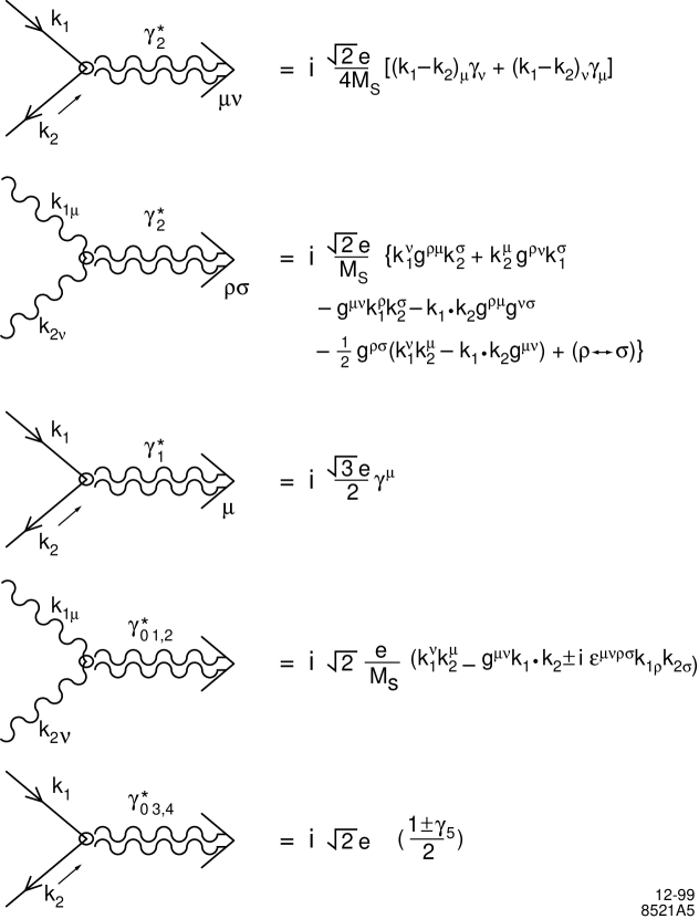
Figure 7: Feynman rules for the coupling of the SR resonances at $M=M_{S}$ in string QED to electron and photon pairs.

From these expressions, we can compute the width of the resonances. For the scalar SR resonances,

$$\Gamma_{01}=\Gamma_{02}={\alpha\over 4}M_{S}\ ,\qquad\Gamma_{03}=\Gamma_{04}={\alpha\over 2}M_{S}\ .$$ (39)

For the vector resonance,

$$\Gamma_{1}={\alpha\over 4}M_{S}\ ,$$ (40)

with equal contributions from decays to $e^{-}_{R}e^{+}_{L}$ and $e^{-}_{L}e^{+}_{R}$. For the spin 2 resonance,

$$\Gamma_{2}(e^{+}e^{-})=\Gamma_{2}(\gamma\gamma)={\alpha\over 20}M_{S}\ ,\qquad\Gamma_{2}={\alpha\over 10}M_{S}\ ,$$ (41)

again with equal contributions from $e^{-}_{R}e^{+}_{L}$ and $e^{-}_{L}e^{+}_{R}$. The production cross sections can be derived from these formulae using, for example

$$\sigma(e^{+}e^{-}\to\gamma^{*}_{J})=4\pi^{2}(2J+1){\Gamma(\gamma_{J}^{*}\to e^{+}e^{-})\over M_{S}}\delta(s-M_{S}^{2})\ .$$ (42)

In $e^{+}e^{-}$ collisions, one currently has data available only up to 200 GeV. In quark-antiquark processes, however, collision energies up to 1 TeV and above are available in the Tevatron data. Thus, it is important to generalize this analysis to $q\overline{q}$ collisions so that we can ask whether the SR excitations of the gluon ought to have been seen at the Tevatron. We will now present our first attempt at a generalization of string QED to string QCD. Though this theory will not be completely satisfactory, it will at least allow us to estimate the bound on the string scale from the study of jets at the Tevatron.

Consider, then, a system of four D3-branes with a $U(4)$ gauge symmetry. Represent the gluons of QCD by the gauge bosons of $SU(3)\subset U(4)$, that is, by $3\times 3$ Chan-Paton matrices $t^{a}$. Represent left-handed quarks and antiquarks of one flavor by the $U(4)$ matrices

$$(t^{i})_{pq}={1\over\sqrt{2}}\delta^{i}_{p}\delta^{4}_{q}\ ,\qquad(\overline{t}^{i})_{pq}={1\over\sqrt{2}}\delta^{i}_{q}\delta^{4}_{p}\ .$$ (43)

Ideally, we would like to make an orbifold projection of the $U(4)$ theory onto a theory which contained only these quarks and gluons at the massless level. Unfortunately, this is not possible, because the commutator $[t^{i},\overline{t}^{j}]$ includes not only a linear combination of the $t^{a}$ but also the $U(1)$ generator

$$t_{4}={1\over\sqrt{24}}\pmatrix{1&&&\cr&1&&\cr&&1&\cr&&&-3\cr}\ .$$ (44)

Thus, this massless $U(1)$ gauge boson will also appear in quark-quark scattering amplitudes.

Keeping this problem in mind, we compute the amplitude for $q_{L}\overline{q}_{R}$ scattering using (8). Only the first line has a nonzero Chan-Paton factor, which equals

$${\mbox{\rm tr}}[t^{i}\overline{t}^{j}t^{k}\overline{t}^{\ell}+\overline{t}^{\ell}t^{k}\overline{t}^{j}t^{i}] = {1\over 4}\left\{\delta^{jk}\delta^{\ell i}+\delta^{k\ell}\delta^{ij}\right\}$$ (45)

$$= {1\over 2}\left\{(t^{a})_{ji}(t^{a})_{\ell k}+{2\over 3}\delta^{ji}\delta^{\ell k}\right\}\ .$$

In the last line, the first term corresponds to color octet exchange in the $s$-channel, and the second term to exchange of a $U(1)$ boson corresponding to the generator (44). To make our estimate, we will drop the $U(1)$ piece and then factorize the color octet piece of the amplitude as above. This gives

$${\cal A}(q_{L}^{i}\overline{q}_{R}^{j}\to q_{L}^{\ell}\overline{q}_{R}^{k})=-2g^{2}{u^{2}\over st}(t^{a})_{ji}(t^{a})_{\ell k}\cdot{\cal S}(s,t)\ ,$$ (46)

which implies:

$${\cal A}(q_{L}^{i}\overline{q}^{j}_{R}\to g_{1}^{*a}) = \sqrt{{3\over 2}}gM_{S}(t^{a})_{ji}\epsilon_{-}^{\mu}\ ,$$

$${\cal A}(q^{i}_{L}\overline{q}^{j}_{R}\to g_{2}^{*a}) = \sqrt{{1\over 2}}gM_{S}(t^{a})_{ji}\cdot{1\over\sqrt{2}}[\epsilon_{-}^{\mu}\epsilon_{0}^{\nu}+\epsilon_{-}^{\nu}\epsilon_{0}^{\mu}]\ ,$$ (47)

and similarly for $q_{R}^{i}\overline{q}^{j}_{L}$. The result is just what we would have obtained by replacing $e$ by $g$ and adding an $SU(3)$ color matrix in the Feynman rules of Figure 7. From these matrix elements, we can compute the production cross sections from unpolarized $q\overline{q}$ initial states:

$$\sigma(q\overline{q}\to g_{1}^{*})={4\pi^{2}\alpha_{s}\over 3}\delta(s-M_{S}^{2})\ ,\qquad\sigma(q\overline{q}\to g_{2}^{*})={4\pi^{2}\alpha_{s}\over 9}\delta(s-M_{S}^{2})\ ,$$ (48)

so that

$$\sigma(q\overline{q}\to g^{*})={16\pi^{2}\alpha_{s}\over 9}\delta(s-M_{S}^{2})\ .$$ (49)

The result (49) can be compared to the cross section for producing the axigluon [39] and coloron [40], hypothetical massive vector or axial vector bosons that couple to $q\overline{q}$ with the QCD coupling strength. In either case, the cross section is

$$\sigma(q\overline{q}\to V)={16\pi^{2}\alpha_{s}\over 9}\delta(s-M_{S}^{2})\ .$$ (50)

Then we can use experimental constraints on these objects to place a direct experimental bound on the string scale. A recent paper by the CDF collaboration has searched for the presence of a narrow resonance in the two-jet invariant mass distribution in $p\overline{p}$ collisions at the Tevatron [41]. The CDF collaboration does not find evidence for such a resonance and puts a lower limit of 980 GeV (at 95% conf.) on the axigluon or coloron mass. Naively, we should have the same limit on $M_{S}$. Several uncertain factors appear in this comparison, however. On the negative side, the events with $g_{2}^{*}$ have an angular distribution which is more peaked toward the beam axis, and so the acceptance for these events should be lower. The angular distribution for the $g_{1}^{*}$ events is identical to that from the axigluon or coloron. On the positive side, we have ignored scalar gluon resonances and the production of $g_{1}^{*}$ and $g_{2}^{*}$ by gluons. Thus, we might say that the CDF limit constraints the string scale $M_{S}$ to be greater than approximately 1 TeV. If we convert this limit to a limit on the quantum gravity scale using the second line of (3), we find that $M>1.6$ TeV.

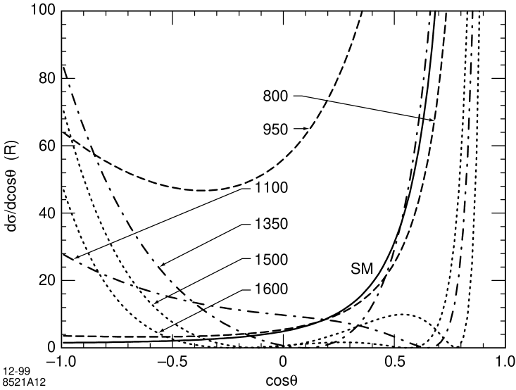
Figure 8: Differential cross section for Bhabha scattering in our string model, with $M_{S}=1$ TeV, at a sequence of center of mass energies that interleave the first few resonances. The cross sections are given in units of $R=4\pi\alpha^{2}/3s$. The number next to each curve indicates the energy. The various line types show: solid, Standard Model prediction; dashed, $E_{\mbox{\scriptsize CM}}<M_{S}$; dot-dash, $M_{S}<E_{\mbox{\scriptsize CM}}<\sqrt{2}M_{S}$; dotted, $\sqrt{2}M_{S}<E_{\mbox{\scriptsize CM}}<\sqrt{3}M_{S}$.

The sensitivity to SR resonances in quark and gluon scattering will increase dramatically when the LHC begins operation. The sensitivity of higher-energy hadron colliders to the axigluon was estimated some time ago by Bagger, Schmidt, and King [42]. Scaling their results to the LHC energy, we expect that the LHC could put a limit of about 5 TeV on the axigluon mass, and a comparable limit on $M_{S}$. Using (3), this would correspond to a limit $M>8$ TeV. These values are sufficiently high that string resonances ought to be discovered at the LHC if the low quantum gravity scale is connected to the mechanism of electroweak symmetry breaking as suggested by ADD [1].

To conclude this section, we discuss what happens when we probe even higher energies, above the scale of the first SR resonance. When $s>M_{n}^{2}$, the expression (11) has a zero at $t=-(s-M_{n}^{2})$. Thus, above the first resonance, there is one zero in $\cos\theta$, above the second resonance, there are two zeros, and so forth. This leads to an angular distribution of the sort produced by diffractive scattering. In Figure 8, we plot the differential cross section for Bhabha scattering, from (28), for a sequence of energies that interleave the SR resonances.

It is well-known from the old string literature that the differential cross sections at very high energy have the form of a narrow diffractive peak. Indeed, using Stirling’s formula to evaluate ${\cal S}(s,t)$ in the limit $s\to\infty$ and fixed angle, we find [9]

$${\cal S}(s,t)\sim\exp[-{\alpha^{\prime}}sf(\cos\theta)]\ ,$$ (51)

where $f(\theta)$ is the positive function

$$f(c)=-{1+c\over 2}\log{1+c\over 2}-{1-c\over 2}\log{1-c\over 2}\ .$$ (52)

However, at intermediate energies, the large positive deviation in the backward direction is also an important part of the string signature. As $\cos\theta\to-1$,

$$\bigl{|}{\cal S}(s,t)\bigr{|}^{2}\to\left({\pi{\alpha^{\prime}}s\over\sin\pi{\alpha^{\prime}}s}\right)^{2}\ .$$ (53)

Thus for increasing $s$ there is a larger enhancement, but in a narrower region of backward angles.

5 Stringy corrections to $e^{+}e^{-}\to\gamma G$

Our toy model includes the process of graviton emission in electron-positron annihilation, $e^{+}e^{-}\to\gamma G$. This process gives a missing-energy signature which becomes significant when the center-of-mass energy of the annihilation approaches the gravitational scale $M$. The process has been used by the LEP 2 experiments to put constraints on the size of large extra dimensions. In this section, we study the stringy corrections to this process.

To begin, we recall that the leading contribution to this process at low energy is model-independent. The calculation uses only the fact that a graviton—even a KK excitation—couples to the energy-momentum tensor of matter [43]. The coupling has the usual 4-dimensional gravitational strength. From this, one finds that the polarized differential cross section for the process $e^{-}_{L}e^{+}_{R}\to\gamma G$, for production of a given KK excitation of mass $m$, is given by [3, 4]

$${d\sigma\over d\cos\theta}\biggr{|}_{\mbox{\scriptsize ft}} = {\pi\alpha G_{N}\over 1-m^{2}/s}\Biggl{[}(1+\cos^{2}\theta)\left(1+\bigl{(}{m^{2}\over s}\bigr{)}^{4}\right)$$ (54)

$$+\left({1-3\cos^{2}\theta+4\cos^{4}\theta\over 1-\cos^{2}\theta}\right){m^{2}\over s}\left(1+\bigl{(}{m^{2}\over s}\bigr{)}^{2}\right)+6\cos^{2}\theta\bigl{(}{m^{2}\over s}\bigr{)}^{2}\Biggr{]}\ .$$

To obtain the full cross-section for graviton emission at a given collision energy, we need to sum over all the modes whose emission is kinematically allowed. The resulting cross-section behaves as $\sigma\sim s^{n/2}/M^{n+2}$. This expression grows with $s$; if it were valid for all $s$, it would violate unitarity. We will see that string theory supplies an appropriate form factor to cut off this dependence.

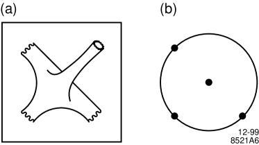
Figure 9: Schematic illustration and world-sheet diagram of the scattering process involving three open strings on a D-brane and one closed string in the bulk.

In our stringy toy model, the graviton is a part of the closed string massless spectrum, while the electrons and photons are described by massless states of open strings. Therefore, to study the process $e^{+}e^{-}\to\gamma G$ we consider the string scattering amplitude involving three open strings and a closed string. The calculation of this amplitude is very similar to the calculation of the four open-string scattering presented in Section 3. The amplitude is given by

$${\cal M}(1,2,3,G)=gM(1,2,3,G)\,\,{\mbox{\rm tr}}([t^{1},t^{2}]t^{3}),$$ (55)

where we need to substitute for each $t^{i}$ the appropriate matrix from (5). To evaluate the ordered amplitude $M(1,2,3,G)$, we map the string worldsheet in Fig. 9 (a) onto a disc, and then into the upper half plane. The three open string vertex operators have to be placed on the boundary; the closed string vertex operator can sit anywhere inside the upper half plane. Then, the ordered amplitude is

$$M(1,2,3,G)={1\over{{\alpha^{\prime}}}^{2}}X^{2}\int_{{\cal C}^{+}}d^{2}z\left<\prod_{i=1}^{3}{\cal V}_{q_{i}}(x_{i},k_{i}){\cal V}_{q_{G}}(z,\overline{z},k_{G})\right>\ ,$$ (56)

where ${\cal V}_{q_{i}}(x_{i})$ is the vertex operator of the open string state $i$, and ${\cal V}_{q_{G}}(z,\overline{z})$ is the vertex operator of the graviton. The open string vertex operators are placed on the real axis at $x_{i}=0,1,X$, with $X$ to be fixed and sent to $\infty$. The integral is taken over the upper half plane ${\cal C}^{+}$. Just as in Section 3, we perform the doubling trick, extending the definitions of the fields to the full complex plane; then the open string vertex operators are given by (17) and (18). The closed string vertex operator in the 0 picture takes the form

$${\cal V}_{0,0}^{\mu\lambda}(z,\overline{z},k) = -{\kappa\over\pi{\alpha^{\prime}}}D^{\lambda}_{\,\nu}\left(\partial X^{\mu}(z)+ik\cdot\psi(z)\psi^{\mu}(z)\right)e^{ik\cdot X(z)}$$ (57)

$$\cdot\left(\partial X^{\nu}(\overline{z})+iDk\cdot\psi(\overline{z})\psi^{\nu}(\overline{z})\right)e^{iDk\cdot X(\overline{z})},$$

where $D^{\mu}_{\,\nu}=1$ for $\mu=\nu=0..3$, $D^{\mu}_{\,\nu}=-1$ for $\mu=\nu=5..10$, and $D^{\mu}_{\,\nu}=0$ for $\mu\not=\nu$. Using these vertex operators and the correlation functions given in (16) and (19), the amplitude (56) can be evaluated. In this calculation, one encounters integrals of the form

$$I_{0}(a,b,c) = \int_{{\cal C}^{+}}d^{2}z\,|z|^{a}\,|1-z|^{b}\,(z-\overline{z})^{c},$$

$$I_{1}(a,b,c) = \int_{{\cal C}^{+}}d^{2}z\,|z|^{a}\,|1-z|^{b}\,(z-\overline{z})^{c}\,(z+\overline{z}),$$ (58)

with arbitrary $a,b,c.$ Using the representation

$$|z|^{a}={1\over\Gamma(-a/2)}\int_{0}^{\infty}t^{-a/2-1}e^{-t|z|^{2}}dt$$ (59)

these integrals can be evaluated. The results are

$$I_{0}(a,b,c) = (2i)^{c}{\sqrt{\pi}\over 2}\Gamma\left(-1-(a+b+c)/2\right)$$

$$\hskip 28.45274pt\cdot{\Gamma\left((1+c)/2\right)\Gamma\left(1+(b+c)/2\right)\Gamma\left(1+(a+c)/2\right)\over\Gamma(-a/2)\Gamma(-b/2)\Gamma\left(2+(a+b)/2+c\right)}\ ;$$

$$I_{1}(a,b,c) = 2{2+a+c\over 4+a+b+2c}I_{0}(a,b,c).$$ (60)

We find that the individual amplitudes contributing to (54) are all multiplied by a common factor

$${\cal F}(s,t,u,m^{2}) = {1\over\sqrt{\pi}}e^{-(\log 2){\alpha^{\prime}}m^{2}}\Gamma(\frac{1}{2}-\frac{1}{2}{\alpha^{\prime}}m^{2})$$ (61)

$$\hskip-56.9055pt\cdot{\Gamma(1-\frac{1}{2}{\alpha^{\prime}}s)\Gamma(1-\frac{1}{2}{\alpha^{\prime}}t)\Gamma(1-\frac{1}{2}{\alpha^{\prime}}u)\over\Gamma(1+\frac{1}{2}{\alpha^{\prime}}(s-m^{2}))\Gamma(1+\frac{1}{2}{\alpha^{\prime}}(t-m^{2}))\Gamma(1+\frac{1}{2}{\alpha^{\prime}}(u-m^{2}))}\ .$$

An analogous result holds for the process $gg\rightarrow gG$: To obtain the string theory amplitude, we just multiply the field theory answer by the same prefactor (61). This result is in agreement with the calculation of Dudas and Mourad [14]. We believe, but we have not been able to show, that the relation among amplitudes is a consequence of the $N=4$ supersymmetry of the underlying model. The field-theory cross section formula (54) is then modified by

$${d\sigma\over d\cos\theta}={d\sigma\over d\cos\theta}\biggr{|}_{\mbox{\scriptsize ft}}\cdot\left|{\cal F}(s,t,u,m^{2})\right|^{2}\ .$$ (62)

The expression (61) has an interesting pole structure [14]. The poles in the $s$ channel occur for $s=2nM_{S}^{2}$, and correspond to producing SR states with an even excitation number. The SR states with an odd excitation number cannot decay into a graviton and an open string massless state. On the other hand, these states can mix with the graviton, leading to the appearance of extra poles at $m^{2}=(2n+1)M_{S}^{2}$. These poles were also observed by Hashimoto and Klebanov [24] in their calculation of the gluon-gluon-graviton vertex. Their presence is essential for the correct factorization properties of the form factor (61).

The form factor (61) expresses the way in which the amplitudes for KK graviton emission are cut off in all relevant high-energy limits. Assume that the kinematic variables are sufficiently far away from any of the poles in (61). (Near the poles, the effects of finite width of the resonances have to be taken into account. This is beyond the scope of our analysis here.) For the radiation of state of very high mass, we can evaluate ${\cal F}$ at the threshold $s=m^{2}$, $t=u=0$, and then take $m^{2}$ large. Using Stirling’s formula, we find

$${\cal F}\sim\exp[-(\log 2){\alpha^{\prime}}m^{2}]\ .$$ (63)

In the limit of fixed mass, $s\to\infty$, and fixed angle, we find

$${\cal F}\sim\exp[-{\alpha^{\prime}}sf(\cos\theta)]\ ,$$ (64)

where $f(c)$ is the function defined in (52). In the high-energy limit in which $s,t,u,m^{2}$ all become large together, we find the more complicated formula

$${\cal F}\sim\exp[-\frac{1}{2}{\alpha^{\prime}}sf(x,\cos\theta)]\ ,$$ (65)

where $x=m^{2}/s$ and $f(x,c)$ is given by

$$f(x,c) = x\log{4x}-(1-x){(1+c)\over 2}\log{(1+c)\over 2}-(1-x){(1-c)\over 2}\log{(1-c)\over 2}$$ (66)

$$-({(1+c)\over 2}+x{(1-c)\over 2})\log({(1+c)\over 2}+x{(1-c)\over 2})$$

$$-({(1-c)\over 2}+x{(1+c)\over 2})\log({(1-c)\over 2}+x{(1+c)\over 2})\ .$$

The function $f(x,c)$ is positive for the allowed values of $c$ and $x$, even though this property is not manifest in (66). Thus, the string correction (61) gives a form factor suppression in all hard-scattering regions.

Recently, Bando et al. [44] have pointed out that high-mass graviton emission from a brane is suppressed by a form factor effect due to brane recoil. The formula they propose is

$${\cal F}\sim\exp[-\frac{1}{2}{\Lambda_{S}^{2}\over\tau_{3}}m^{2}]\ ,$$ (67)

where $\tau_{3}$ is the brane tension and $\Lambda_{S}$ is a cutoff scale which should be of order $M_{S}$. The expression in the exponent is smaller than that in (63) by a factor of order $g_{YM}^{2}$. In weak-coupling Type IIB string theory, brane recoil is described by the emission of scalars in the $N=4$ gauge multiplet associated with brane. With the orbifold projection described in Section 2, there is one scalar $\phi^{3}$ that survives and remains in the spectrum. This scalar does not couple to the QED state in the field theory limit, but it does couple through higher-dimension operators. However, these couplings are proportional to one factor of $g_{YM}$ in the amplitude for each $\phi^{3}$ emitted. These inelastic processes deplete the cross section for elastic $G$ emission without $\phi^{3}$ emission and should lead to a form factor suppression of the form $\exp[-cg_{YM}^{2}m^{2}/M_{S}^{2}]$. This is in agreement with the result of [44]. However, we see from (63) that there is a parametrically more important source for the form factor, the intrinsic non-pointlike nature of the states in string theory. We should note that the numerical coefficient in the formula (4) for the brane tension is quite small, so that effects of the size (67) might nevertheless be relevant.

In our study of open-string scattering, we saw that the form factor cutoff of string amplitudes is important only at very high energy. At energies of the order of the string scale, a much more important phenomenon is the enhancement of scattering cross sections through the effect of SR resonances. We have seen that the amplitudes for graviton emission contain the series of SR poles at $s=2nM_{S}^{2}$ and $m^{2}=(2n+1)M_{S}^{2}$. Thus, string theory predicts an enhancement of the rate for graviton emission processes such as $e^{+}e^{-}\to\gamma G$ through resonant processes such as

$$e^{+}e^{-}\to\gamma^{**}\to\gamma G\ ,\quad e^{+}e^{-}\to\gamma\gamma^{*}_{1,2}\to\gamma\gamma G\ .$$ (68)

Typically, the resonances would be seen more clearly in $e^{+}e^{-}$ or $q\overline{q}$ elastic scattering. However, the resonant production of missing-energy events would be an important confirmation that the observed resonances were a manifestation of quantum gravity with large extra dimensions.

6 Stringy corrections to $\gamma\gamma$ scattering

In this section, we address the question of the relative strengths of the effective operators in the low energy theory mediated by virtual SR and KK exchanges. At the end of Section 1, we argued, on very general grounds, that in any weakly coupled string theory the SR-mediated operators are expected to dominate. Here, we will substantiate this claim by an explicit calculation.

6.1 Tree amplitude

It is important to note that, unlike renormalizable field theory, string theory gives a nonzero contribution to the $\gamma\gamma$ scattering amplitude at the tree level. To compute this amplitude, we follow the procedure outlined in Section 3. We find

$${\cal A}(\gamma_{R}\gamma_{R}\to\gamma_{R}\gamma_{R})=-e^{2}s^{2}\left[{1\over st}{\cal S}(s,t)+{1\over su}{\cal S}(s,u)+{1\over tu}{\cal S}(t,u)\right]\ ,$$ (69)

where ${\cal S}(s,t)$ is given by (11). The helicity amplitudes for $\gamma_{R}\gamma_{L}\to\gamma_{R}\gamma_{L}$ and $\gamma_{L}\gamma_{L}\to\gamma_{L}\gamma_{L}$ can be obtained from (69) by crossing. All other helicity amplitudes vanish.

The expression (69) must vanish in the field theory limit ${\alpha^{\prime}}\to 0$. This is easily seen as a consequence of $s+t+u=0$. Using a higher–order expansion of ${\cal S}$, as in (21), we obtain

$${\cal A}(\gamma_{R}\gamma_{R}\to\gamma_{R}\gamma_{R})={\pi^{2}\over 2}e^{2}{s^{2}\over M_{S}^{4}}+\cdots\ ,\qquad{\cal A}(\gamma_{R}\gamma_{L}\to\gamma_{R}\gamma_{L})={\pi^{2}\over 2}e^{2}{u^{2}\over M_{S}^{4}}+\cdots\ .$$ (70)

This result can be compared to the $\gamma\gamma\to\gamma\gamma$ amplitude induced by KK graviton exchange. Using the effective Lagrangian (30), it is straightforward to see that [45, 46]

$${\cal A}_{\rm KK}(\gamma_{R}\gamma_{R}\to\gamma_{R}\gamma_{R})=16{\lambda\over M_{H}^{4}}s^{2}\ ,\qquad{\cal A}_{\rm KK}(\gamma_{R}\gamma_{L}\to\gamma_{R}\gamma_{L})=16{\lambda\over M_{H}^{4}}u^{2}\ .$$ (71)

These expressions have exactly the same form as (70), and this must be so, because there is only one gauge-invariant, parity-conserving dimension 8 operator which contributes to $\gamma\gamma\to\gamma\gamma$. However, the scale $M_{H}$ in (71) is different from the string scale that appears in (70). We have already remarked in Section 4 that the relation between $M_{S}$ and $M_{H}$ can be obtained explicitly in our string model, and that in a weakly-coupled string theory the effect of KK graviton exchanges (71) is subdominant to the SR exchanges (70). In the next section, we will derive that result.

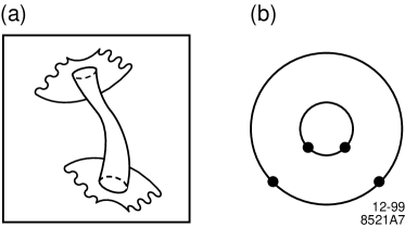
Figure 10: Schematic illustration and world-sheet diagram for open string scattering via a closed string exchange.

6.2 Loop amplitude

In string theory, the graviton exchange proper arises at the next order in perturbation theory. The graviton is a closed-string state. It first appears in open-string perturbation theory through the 1-loop diagram shown in Figure 10 [13]. In this section, we will compute this diagram and show that it contains a piece which has the form of the one-graviton exchange amplitude. Some other properties of this diagram have recently been analyzed in [14].

In the covariant formulation of string theory [9, 26], the open string loop amplitude shown in Figure 10 is computed in terms of correlation functions of vertex operators placed on the two boundaries. It is convenient to conformally map the annulus shown in Figure 10(b) into a cylinder, represented by a rectangle in the complex plane

$$0\leq\Re w\leq\pi\ ,\qquad 0\leq\Im w\leq 2\pi t\ ,$$ (72)

periodically connected with the identification $w\cong w+2\pi it$. The boundaries of the annulus are mapped to the lines $\Re w=0$ and $\Re w=\pi$. The parameter $t$ is a modulus which must be integrated over the whole range $0<t<\infty$.

The complete four-point open string amplitude is a sum of ordered amplitudes in which the four vertex operators are placed on the boundaries in all possible ways. The open strings on a D-brane and the Type IIB closed strings are oriented, so we do not need to consider non-orientable worldsheets such as the Mobius strip. Thus,

$${\cal A}_{\rm 1-loop}= g^{4}A_{\rm p}(1,2,3,4)\cdot{\mbox{\rm tr}}[t^{1}t^{2}t^{3}t^{4}]+{\rm\,\,perms\,\,}+$$ (73)

$$g^{4}A_{\rm np}(1,2;3,4)\cdot{\mbox{\rm tr}}[t^{1}t^{2}]{\mbox{\rm tr}}[t^{3}t^{4}]+{\rm\,\,perms}.$$ (75)

This equation is the analogue of the tree-level color decomposition in (8). Only the second line, the ‘non-planar’ amplitude, has the correct color structure to represent graviton exchange. We will show that the first term in the second line, which we denote ${\cal A}_{Gs}$, contains the contribution of a virtual graviton exchanged in the $s$-channel.

The explicit expression for ${\cal A}_{Gs}$ is

$${\cal A}_{Gs}=g^{4}{\mbox{\rm tr}}[t^{1}t^{2}]{\mbox{\rm tr}}[t^{3}t^{4}]\int{dt\over t}\left[\prod_{i=1}^{4}\int_{0}^{2\pi t}dy_{i}\right]$$

$$\cdot Z_{x}^{p}\sum_{\lambda}Z_{\lambda}\left<\prod_{i=1}^{4}\epsilon_{i}\cdot{\cal V}_{0}(w_{i},k_{i})\right>_{\lambda}\ ,$$ (76)

where $Z_{x}^{p}$ denotes the partition function of the worldsheet bosons $X^{\mu}$ and the anticommuting ghosts, and $Z_{\lambda}$ denotes the partition function of the worldsheet fermions $\psi^{\mu}$ and the commuting ghosts. The expectation value is correspondingly assumed to be computed only from field contractions, excluding the partition functions. The parameter $\lambda$ denotes the periodicities of the worldsheet fermions. As we stated in Section 2, we will carry out our computations in this section in the original $N=4$ supersymmetric Type IIB theory. Thus, we will sum only over uniform periodic and antiperiodic boundary conditions for the world-sheet fermions around each of the two cycles. The vertex operators are placed at

$$w_{1}=iy_{1}\ ,\quad w_{2}=iy_{2}\ ,\quad w_{3}=\pi+iy_{3}\ ,\quad w_{4}=\pi+iy_{4}\ .$$ (77)

We will check the overall normalization of this expression in Section 6.3.

The easiest way to account for the boundary conditions on the worldsheet fermions is to extend their definitions to $\pi\leq\Re w\leq 2\pi$. On this extended worldsheet, the fermions are holomorphic, and their possible periodicities and correlators are the same as for a torus with modulus $it$. For the worldsheet bosons, the boundary conditions can be described using the method of image charges. For the fields located on the boundary and satisfying Neumann boundary conditions the correlator is the same as that for a torus with modulus $it$, with an extra factor of 2 from the image fields. The correlators necessary for our calculation are listed explicitly in Appendix B.

For the computation of this section, we will be interested in the contribution to the amplitude from bosonic closed string states propagating up the cylinder. These states have fermions antiperiodic around the cylinder, that is, in the direction of $\Im w$. Both boundary conditions in the direction of $\Re w$ are needed to enforce the GSO projection [9]. We will refer to the partition functions for the sectors antiperiodic in the imaginary direction and antiperiodic/periodic in the real direction as $Z^{A}_{A}$/$Z^{A}_{P}$ and use a similar notation for the correlation functions. In Section 6.3, we will also consider the contribution from bosonic open string states propagating around the cylinder. These states have fermions with boundary conditions antiperiodic in the real direction. The computation will involve the partition functions $Z^{A}_{A}$/$Z^{P}_{A}$ and the analogous correlators.

For the cylinder amplitude, the superconformal charges satisfy $\sum_{i}q_{i}=0$. Thus, we will write all four vertex operators in the 0 picture. We will use the explicit form

$${\cal V}_{0}^{\mu}(k_{i})=(i\dot{X}^{\mu}+{\alpha^{\prime}}2k\cdot\psi\,\,\psi^{\mu})e^{ik_{i}\cdot X}(w_{i},\overline{w_{i}}),$$ (78)

where the dot denotes a derivative along the boundary. Note that this expression is slightly different from (17) in that the $X$ field has not been split into holomorphic and antiholomorphic components.

The $t$ integration in (76) runs from 0 to $\infty$. However, this domain of integration can be separated into two regions. In the limit of small $t$, the cylinder becomes very long and the amplitude is dominated by light closed-string states. In the limit of large $t$, the cylinder becomes very narrow and the amplitude is dominated by light open-string states. The separation between these two regions is ambiguous, since only their sum is a well-defined gauge-invariant quantity. We parametrize this ambiguity by the integration cutoff $t_{0}$. Below we will show that the small-$t$ region reproduces the graviton exchange amplitudes (71), with $M_{H}$ related to the string scale and $t_{0}$. In this calculation, we will use the small-$t$ expansions of the partition functions and correlators. These expressions (given in Appendix B) are valid up to $t\sim\pi$. This suggests that the natural value of the cutoff is $t_{0}\sim\pi$. The expression we will derive for $M_{H}$ will depend on $t_{0}$. This simply makes clear that the loop diagrams of string theory also give other contributions to the dimension 8 terms of the effective Lagrangian. The most important point is that all of these contributions are subleading, suppressed by a power of $g^{2}$ relative to the SR contribution (69).

We now describe the evaluation of the graviton-exchange contribution in (76). For the moment, we consider a D$p$-brane with $p$ arbitrary; later we will specialize to the case $p=3$. Using the small-$t$ expressions of the partition functions and correlators given in Appendix B, we find the expression

$${\cal A}_{Gs} = g^{4}\delta^{12}\delta^{34}\cdot 4^{-{\alpha^{\prime}}s}2^{(7-3p)/2}\pi^{3-p}{{\alpha^{\prime}}}^{(7-p)/2}\cdot\int_{0}^{t_{0}}dtt^{(5-p)/2}\exp({{\alpha^{\prime}}s\over 2}{\pi\over t})$$ (79)

$$\cdot 2\left[\prod_{i=1}^{4}\int_{0}^{1}dY_{i}\right](\sin\pi Y_{12})^{-{\alpha^{\prime}}s}(\sin\pi Y_{34})^{-{\alpha^{\prime}}s}F(Y_{i};\epsilon_{i},k_{i})\hskip 14.22636pt+\hskip 14.22636pt\Delta,$$

where $F$ is a function of external momenta and kinematics which has no $t$ dependence, $Y_{i}=y_{i}/2\pi t$, $Y_{ij}=Y_{i}-Y_{j}$, and $\Delta$ is the contribution to the integral from the large-$t$ region. Explicitly, the function $F$ is given by

$$F=C_{1}+C_{2}\ ,$$ (80)

where

$$C_{1} = \left({1\over 2{\alpha^{\prime}}}\right)^{2}\epsilon_{1}\cdot\epsilon_{2}\epsilon_{3}\cdot\epsilon_{4}\sin^{-2}\pi Y_{12}\sin^{-2}\pi Y_{34},$$

$$C_{2} = {k_{1}\cdot k_{4}}\bigl{(}2k_{1}\cdot k_{4}\,\epsilon_{1}\cdot\epsilon_{2}\,\epsilon_{3}\cdot\epsilon_{4}+2\epsilon_{1}\cdot\epsilon_{2}\,(k_{1}\cdot\epsilon_{3}\,k_{3}\cdot\epsilon_{4}+\epsilon_{3}\cdot k_{4}\,k_{2}\cdot\epsilon_{4})$$ (81)

$$\hskip 56.9055pt+2\epsilon_{3}\cdot\epsilon_{4}\,(k_{1}\cdot\epsilon_{2}\,\epsilon_{1}\cdot k_{3}+\epsilon_{1}\cdot k_{2}\,\epsilon_{2}\cdot k_{4})\bigr{)}.$$

Since we are only interested in the $s\rightarrow 0$ limit of the amplitude, in (81) we have dropped the terms which do not contribute in this limit.

The small-$t$ contribution in (79) factorizes into two integrals, the modulus intergal in the first line and the coordinate integral in the second line. The coordinate integral can be easily evaluated. In this calculation, one encounters two simple integrals,

$$I_{1}=\int_{0}^{1}dY_{1}\int_{0}^{1}dY_{2}(\sin\pi Y_{12})^{-2-{\alpha^{\prime}}s},$$ (82)

and

$$I_{2}=\int_{0}^{1}dY_{1}\int_{0}^{1}dY_{2}(\sin\pi Y_{12})^{-{\alpha^{\prime}}s}.$$ (83)

Evaluating these integrals in the limit ${\alpha^{\prime}}s\rightarrow 0$ yields $I_{1}=0$, $I_{2}=1$. Therefore, in this limit we have

$$2\left[\prod_{i=1}^{4}\int_{0}^{1}dY_{i}\right](\sin\pi Y_{12})^{-{\alpha^{\prime}}s}(\sin\pi Y_{34})^{-{\alpha^{\prime}}s}F(Y_{i};\epsilon_{i},k_{i})=2C_{2}.$$ (84)

One can show that this expression is identical to the matrix element of the square of the photon energy-momentum tensor, $T^{\mu\nu}(1,2)T_{\mu\nu}(3,4)$. This means that in this limit, this process is accurately described by the effective Lagrangian (30). The integral over the modulus $t$ then determines the coefficient of this operator.

The modulus integral can be rewritten in a form reminiscent of a massive graviton propagator from field theory. To do this, we change the integration variable to $v=1/t$, and use the identity

$$v^{(p-9)/2}=\left({{\alpha^{\prime}}\over 2}\right)^{(9-p)/2}\int d^{9-p}m\exp(-{\pi{\alpha^{\prime}}m^{2}\over 2}v)\ .$$ (85)

Performing the $v$ integration, we find

$$\int_{0}^{t_{0}}dtt^{(5-p)/2}\exp({{\alpha^{\prime}}s\over 2}{\pi\over t})=-\left({{\alpha^{\prime}}\over 2}\right)^{(7-p)/2}{1\over\pi}\int d^{9-p}m{1\over s-m^{2}}\exp\bigl{(}{\pi{\alpha^{\prime}}(s-m^{2})\over 2}v_{0}\bigr{)},$$ (86)

where $v_{0}=1/t_{0}$. When both $s$ and $m^{2}$ are small compared to $1/{\alpha^{\prime}}$, the integrand in (86) is just the field theory propagator. We have already pointed out that the virtual graviton exchange cannot be analyzed within effective field theory; technically, this results from the divergence of the KK mass integration in the region of high $m$. The integral in (86), however, is finite, due to the exponential suppression for ${\alpha^{\prime}}m^{2}\gg 1$. This finite coefficient gives the scale $M_{H}$ in (30).

Evaluating the integral (86) for $s=0$ and assembling the pieces, we obtain as the leading term in the low-energy expansion of the small-$t$ integral of (79)

$${\cal A}_{Gs}=g^{4}\delta^{12}\delta^{34}\cdot 2^{(9-3p)/2}\pi^{(13-3p)/2}(\pi v_{0})^{(p-7)/2}{{\alpha^{\prime}}}^{(7-p)/2}{1\over 7-p}\cdot T^{\mu\nu}(1,2)T_{\mu\nu}(3,4)+\ldots\ .$$ (87)

Now set $p=3$. The amplitude (87) can be reproduced by the effective Lagrangian (30), provided that we identify

$${8\over M_{H}^{4}}=g^{4}{\pi^{2}\over 4}{1\over M_{S}^{4}}\cdot(\pi v_{0})^{-2},$$ (88)

and use $\lambda=+1$ in (30). As we have explained above, for a numerical estimate we can evaluate this expression with $v_{0}\sim 1/\pi$. This gives

$${1\over M_{H}^{4}}\sim{\pi^{2}\over 32}{g^{4}\over M_{S}^{4}}.$$ (89)

As expected, the relation is of the form (31), with an additional suppression from the numerical coefficient on the right-hand side. Substituting this value of $M_{H}$ into (71), we confirm that this contribution is subdominant with respect to the SR exchange amplitude (69).

6.3 Normalization

There is another reason that we must analyze the one-loop diagram, and that is to find the relation between the effective Newton constant or the gravity scale $M$ and the more fundamental string theory parameters $g$ and ${\alpha^{\prime}}$. We have already quoted this relation in (2). In this section, we will give the derivation. Once again, our analysis will be done for the toy case of an $N=4$ supersymmetric D-brane theory.

Our procedure is illustrated in Figure 11. We will first take the $t\to\infty$ limit of the cylinder and relate this to a loop diagram of Yang-Mills field theory. This will determine the normalization of the diagram. Then we will take the $t\to 0$ limit to identify the graviton exchange. In this section, we will give what we consider the shortest route through this analysis, considering a two-point function in the first part of the calculation rather than a four-point function, and, in the second part, considering only one fairly simple structure in the gravitation interaction.

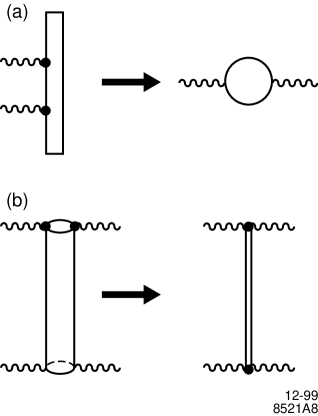
Figure 11: Limits of the cylinder diagram which must be compared to derive the normalization of the graviton exchange contribution: (a) $t\to\infty$; (b) $t\to 0$.

We thus consider first the $t\to\infty$ limit. In principle, we should study the four-point loop diagram. However, it is simpler to analyze the two-point function. The normalizations of these diagrams are related by considering the limit $(k_{1}+k_{2})^{2}\to 0$, in which pairs of vertex operators factorize into single vertex operator insertions as shown in Figure 4. Through this relation, the normalization of (76) is equivalent to the following normalization of the planar two-point loop amplitude shown in Figure 11(a):

$${\cal A}_{2}=g^{2}{\mbox{\rm tr}}[t^{1}t^{2}]{\mbox{\rm tr}}[1]\int{dt\over t}\left[\prod_{i=1}^{2}\int_{0}^{2\pi t}dy_{i}\right]\cdot Z_{x}^{p}\sum_{\lambda}Z_{\lambda}\left<\prod_{i=1}^{2}\epsilon_{i}\cdot{\cal V}_{0}(w_{i},k_{i})\right>_{\lambda}\ ,$$ (90)

where the notations are as in (76) and the two vertex operators are placed at $w_{1}$ and $w_{2}$ in (77).

It is simplest to concentrate on the structure

$$\epsilon_{1}\cdot k_{2}\epsilon_{2}\cdot k_{1}\ .$$ (91)

Looking back to the form (78), we see that this structure arises in two ways in the contraction of vertex operators, from the contraction of the two factors $\dot{X}$ with factors $k\cdot X$ in the exponentials, and from a contraction of the fermionic terms with one another. The correlators for $X$ and $\psi$ should be taken in the limit $t\to\infty$; the appropriate expressions are given in (128). In the two sectors corresponding to bosonic open string states, these terms give

$$\left<\Pi\epsilon\cdot{\cal V}\right>^{A}_{A} \sim \epsilon_{1}\cdot k_{2}\epsilon_{2}\cdot k_{1}\left[{{\alpha^{\prime}}}^{2}(1-2Y)^{2}-4{{\alpha^{\prime}}}^{2}(e^{-\pi tY}+e^{-\pi t(1-Y)})^{2}\right]\ ,$$

$$\left<\Pi\epsilon\cdot{\cal V}\right>^{P}_{A} \sim \epsilon_{1}\cdot k_{2}\epsilon_{2}\cdot k_{1}\left[{{\alpha^{\prime}}}^{2}(1-2Y)^{2}-4{{\alpha^{\prime}}}^{2}(e^{-\pi tY}-e^{-\pi t(1-Y)})^{2}\right]\ ,$$ (92)

where $Y=Y_{12}$ and, for clarity, we have left off the expectation value of the exponentials. Restoring this factor, including the partition functions from (112), and making the cancellations between the two sectors, we find

$${\cal A}_{2} = g^{2}N_{C}\delta^{12}\int^{\infty}_{0}{dt\over t}{64\pi^{2}t^{2}{\alpha^{\prime}}^{2}\over(8\pi^{2}{\alpha^{\prime}}t)^{d/2}}$$ (93)

$$\hskip 36.135pt\cdot\int^{1}_{0}dY\,\epsilon_{1}\cdot k_{2}\epsilon_{2}\cdot k_{1}\left[(1-2Y)^{2}-1\right]\exp[{\alpha^{\prime}}k_{1}\cdot k_{2}(2\pi t)Y(1-Y)]\ ,$$

where we have replaced $(p+1)=d$ and ${\mbox{\rm tr}}[1]=N_{C}$. Now do the $t$ integral. For $d$ close to 4, we obtain,

$${\cal A}_{2} = g^{2}N_{C}\delta^{12}{8\over(4\pi)^{2}}\Gamma\left(2-{d\over 2}\right)\epsilon_{1}\cdot k_{2}\epsilon_{2}\cdot k_{1}\,\int^{1}_{0}dY\,\left[(1-2Y)^{2}-1\right]\ .$$ (94)

As Kaplunovsky [47] pointed out for the analogous closed string calculation, this result can be matched to the computation of the one-loop two-point diagram in Yang-Mills theory in the background-field gauge. The required expressions are given in [48]. The value of this diagram given there, summed over the bosonic content of the $N=4$ supersymmetric Yang-Mills theory (1 vector and 6 scalars), is

$$g^{2}N_{C}\delta^{12}{1\over(4\pi)^{2}}\Gamma\left(2-{d\over 2}\right)(\epsilon_{1}\cdot\epsilon_{2}k_{1}\cdot k_{2}-\epsilon_{1}\cdot k_{2}\epsilon_{2}\cdot k_{1})\,\int^{1}_{0}dY\,\left[8(1-2Y)^{2}-8\right]\ .$$ (95)

In this expression, $Y$ is the Feynman parameter. The first term in the bracket comes from a spin-independent determinant, the second term from the spin operator. The expressions (94) and (95) match. Thus, the normalization assumed in (90) and in (76) is correct.

Now we turn to the $t\to 0$ limit. Here it is simplest to extract the graviton exchange by considering the limit of high-energy scattering with low momentum transfer. That is, we set

$$k_{2}\approx-k_{1}\ ,\qquad k_{4}\approx-k_{3}\ .$$ (96)

Then the usual graviton exchange diagram in four dimensions contains a term

$${\cal A}=-8\pi G_{N}\delta^{12}\delta^{34}(2k_{1}^{\mu}k_{1}^{\nu}){1\over s}(2k_{3\mu}k_{3\nu})=-8\pi G_{N}{t^{2}\over s}\delta^{12}\delta^{34}\ ,$$ (97)

where $s=-(k_{1}+k_{2})^{2}=-(k_{3}+k_{4})^{2}$ and $t=-(k_{1}+k_{3})^{2}$.

In the scattering amplitude of four vector bosons, this term has the structure

$$\epsilon_{1}\cdot\epsilon_{2}\epsilon_{3}\cdot\epsilon_{4}k_{1}\cdot k_{3}k_{1}\cdot k_{3}\ ,$$ (98)

using (96) to replace $k_{2}$ and $k_{4}$.

After close examination of the various terms contributing to (76), one can see that, after the cancellation between the $Z^{A}_{A}$ and $Z^{A}_{P}$ sectors, there is only one source for a term of this structure. That is the contribution in which one takes only the fermionic term in each vertex operator (78) and contracts the $\epsilon\cdot\psi$ operators on the same side of the cylinder and the $k\cdot\psi$ operators across the cylinder. The correlators needd are given in (122) and (127). There are two contractions of this type for each sector. When these two terms are added, all dependence on the $Y_{ij}$ cancels out. The contributions from the two sectors then add constructively. The sum of these terms gives

$${\cal A}_{Gs}=(\epsilon_{1}\cdot\epsilon_{2}\epsilon_{3}\cdot\epsilon_{4}\delta^{12}\delta^{34}t^{2})g^{4}{2(2\pi{\alpha^{\prime}})^{4}\over(8\pi^{2}{\alpha^{\prime}})^{(p+1)/2}}\int^{\infty}_{0}dtt^{(5-p)/2}\left[\frac{1}{2}e^{\pi/4t}\right]^{2{\alpha^{\prime}}s}\ .$$ (99)

One should be careful to note that the $t$ in the prefactor is the Mandelstam invariant, whereas the other factors $t$ represent the modulus of the cylinder.

This expression can be simplified by changing variables from $t$ to $v=1/t$ and then introducing the variable $m$ as in (85). Setting also $p=3$, we arrive at the expression

$${\cal A}_{Gs}=(\epsilon_{1}\cdot\epsilon_{2}\epsilon_{3}\cdot\epsilon_{4}\delta^{12}\delta^{34}t^{2})g^{4}{{{\alpha^{\prime}}}^{4}\over 8\pi}\int d^{6}m{1\over m^{2}-s}\ .$$ (100)

We can convert the integral over $m$ to a discrete sum over KK states in the 6 large extra dimensions of periodicity $2\pi R$ by using the relation

$$R^{6}\int d^{6}m=\sum_{m}\ .$$ (101)

Finally, we may pick off the term in the sum that corresponds to the massless graviton in four dimensions. We then identify

$$8\pi G_{N}={1\over 8\pi}{{\alpha^{\prime}}}^{4}g^{4}R^{-6}\ .$$ (102)

Replacing $G_{N}$ with the fundamental quantum gravity scale $M$ according to (1), we find

$$M^{-8}=\pi\alpha^{2}{{\alpha^{\prime}}}^{4}\ ,$$ (103)

which is equivalent to the promised relation (2).

7 Experimental constraints on the quantum gravity scale

It is useful to compare the constraints on the large extra dimension scenario that we have obtained in this paper through model-dependent string effects to more robust, model-independent constraints. In the introduction, we noted that previous constraints on large extra dimensions have come from two sources, searches for missing energy due to gravitation radiation into the extra dimensions, and searches for contact interactions due to KK graviton exchange. It has become clear in this paper that the possible contact interactions are model-dependent and may not be of purely gravitational origin. So the truly model-independent constraints come only from missing-energy experiments.

In Table 1, we summarize the most important present and future constraints on the quantum gravity scale $M$ from missing-energy searches. This table updates the table presented in [4] and improves upon it in several important respects.

Collider		R / M ($n=2$)	R / M ($n=4$)	R / M ($n=6$)
Present:	SN1987A	$3\times 10^{-5}/50000$	$1\times 10^{-9}/1000$	$6\times 10^{-11}/100$
	LEP 2	$4.8\times 10^{-2}$ / 1200	$1.9\times 10^{-9}$ / 730	$6.8\times 10^{-12}$ / 530
	Tevatron	$5.5\times 10^{-2}$ / 1140	$1.4\times 10^{-9}$ / 860	$4.1\times 10^{-12}$ / 780
Future:	LC	$1.2\times 10^{-3}$ / 7700	$1.2\times 10^{-10}$ / 4500	$6.5\times 10^{-13}$ / 3100
	LHC	$4.5\times 10^{-4}$ /12500	$5.6\times 10^{-11}$ / 7500	$2.7\times 10^{-13}$ / 6000

Table 1: Current and future sensitivities to large extra dimensions from missing-energy experiments. All values for colliders are expressed as 95% confidence exclusion limits on the size of extra dimensions $R$ (in cm) and the effective Planck scale $M$ (in GeV). For the analysis of SN1987A, we give probable-confidence limits.

The first line of Table 1 gives the constraints obtained in [5] from the consistency of the observed neutrino flux from the supernova SN1987A with the predictions of the stellar collapse models. This analysis puts an upper bound on the rate of energy loss through graviton emission. There exist some strong astrophysical bounds on the scale of quantum gravity—for example, [49]—but these depend on assumptions about the cosmological scenario. The constraint from the supernova is different in character. Since we have a reasonable understanding of the composition of a supernova and of the conditions inside its core during collapse, it is possible to calculate the gravitional radiation expected in this process in an unambiguous way. The typical energy of the emitted gravitons is well below a TeV, and so the emission rate calculation uses only the model-independent low-energy limit of the gravitational coupling. It is argued in [5] that, though there are uncertainties in the parameters of the supernova core, the bounds quoted should be accurate to better than a factor of 2. The bound for the case of two large extra dimensions ($n=2$) is surprisingly strong and must be taken seriously. We note that the values given in the remaining lines of the table are more precise 95% confidence exclusion limits available from accelerator experiments.

The second line of the table gives the constraints arising from the process $e^{+}e^{-}\to\gamma+$ (missing) which have been announced by the ALEPH collaboration [50, 19]. Similar constraints on anomalous single photon production have been announced by the other LEP experiments [51, 52, 53].

The third line of the table is derived from a new search for events with one jet and missing $E_{T}$ presented by the CDF collaboration in [54]. Of the five cuts on missing $E_{T}$ presented in this analysis, the analysis based on the cut $E_{T}>200$ GeV turns out to give the best sensitivity. We have applied the formulae in [4] to convert the limit on the cross section to the quoted bounds on $M$. Note that these bounds are very close to the estimates in the “Future Tevatron” line of [4].

The fourth line of the table gives the reach of a 1 TeV $e^{+}e^{-}$ linear collider as computed in [4]. However, in the fifth line, the constraints given in Table 1 for the LHC are much stronger. This is the result of the observation, made in [3], that at the LHC there is a dramatic improvement in signal/background if one makes a very hard $E_{T}$ cut. It is advantageous to move this cut to as high a value as the statistics permit. The results shown here correspond to the analysis in [4] applied to a cut at $E_{T}>1000$ GeV.

For the LHC search, one may worry that the effective field theory used to obtain the bounds in Table 1 breaks down for the collisions of the most energetic partons. In Section 5, we have derived the form factor which describes the modification of the cross sections at high energies due to string theory effects. We have shown that at very high energies, this form factor leads to exponential suppression of the signal cross section. One might expect that the sensitivity of the LHC searches will be somewhat lowered by this effect. However, it turns out that for values of the string scale in the few-TeV range, this effect does not significantly alter the signal rates at LHC. In fact, we find a relatively small effect for typical parton-parton center-of-mass energies and a dramatic enhancement when partons can combine to the SR resonances, due to processes analogous to (68) with an excited gluon or quark intermediate state. In the situation in which these states are present, they would also be seen as resonances in the two-jet invariant mass distribution. We conclude that in either case, whether the resonances are observed or not, the bounds in the last line of Table 1 would not be significantly decreased by stringy physics.

8 Conclusions

In this paper, we have studied the phenomenology of large extra dimensions for the situation in which quantum gravity is represented by a weakly-coupled string theory. We have found that, in this case, the signatures of large extra dimensions which have been considered in the literature up to now are overshadowed by genuine string effects. The first sign of new physics is found in string corrections to Standard Model two-body scattering cross sections, leading to contact interactions due to string resonances and to the dramatic appearance of these resonances at colliders. The fact that these resonances have not yet been observed allows us to put a lower bound on the string scale of about 1 TeV. The corresponding limit on the quantum gravity scale, $M>1.6$ TeV, is much stronger than that of any current accelerator experiment. The next generation of colliders should probe values of the string scale up to 5 TeV and values of the quantum gravity scale above 8 TeV.

The motivation for the idea of large extra dimensions in the work of Arkani-Hamed, Dimopoulos, and Dvali [1] came from the possibility of a natural relation between the weak interaction scale and the scale of quantum gravity. If this possibility is indeed realized, the linear collider and the LHC will carry out experimental measurements of string physics. For many years, physicists have thought of strings as tiny objects and imagined that we could observe them in experiments only in some distant era. It seems now that this era could be close at hand.

ACKNOWLEDGEMENTS

We are grateful to Nima Arkani-Hamed for stimulating this investigation, and to Nicolas Toumbas, who collaborated with us in the early stages of this work. We thank Dimitri Bourilkov for a very useful correspondence concerning the LEP 2 Bhabha scattering data. We also thank Tom Banks, Hooman Davoudiasl, Savas Dimopoulos, Lance Dixon, Ian Hinchliffe, Ann Nelson, and Alex Pomarol for helpful discussions and the Institute for Theoretical Physics at UC Santa Barbara for hospitality. The work of SC was supported in part by the US National Science Foundation under contract PHY–9870115; the work of MP and MEP was supported by the US Department of Energy under contract DE–AC03–76SF00515.

Appendix A Reference formulae for models of contact interactions

In this appendix, we give the explicit expressions for the contact-interaction corrections to Bhabha scattering that are compared in Figures 5 and 6. We also give the first contact-interaction corrections to the $e^{+}e^{-}\to\gamma\gamma$ and $\gamma\gamma\to\gamma\gamma$ amplitudes.

The unpolarized cross section formula for Bhabha scattering can be written in the form

$${d\sigma\over d\cos\theta}={\pi\alpha^{2}\over 2s}\left[u^{2}(|A_{LL}|^{2}+|A_{RR}|^{2})+2t^{2}|A_{RL,s}|^{2}+2s^{2}|A_{RL,t}|^{2}\right]\ ,$$ (104)

where

$$A_{LL} = {1\over s}+{1\over t}+{(\frac{1}{2}-\sin^{2}\theta_{w})^{2}\over\sin^{2}\theta_{w}\cos^{2}\theta_{w}}\left({1\over s-m_{Z}^{2}}+{1\over t-m_{Z}^{2}}\right)+\Delta_{LL}$$

$$A_{RR} = {1\over s}+{1\over t}+{\sin^{2}\theta_{w}\over\cos^{2}\theta_{w}}\left({1\over s-m_{Z}^{2}}+{1\over t-m_{Z}^{2}}\right)+\Delta_{RR}$$

$$A_{RL,s} = {1\over s}-{(\frac{1}{2}-\sin^{2}\theta_{w})\over\cos^{2}\theta_{w}}{1\over s-m_{Z}^{2}}+\Delta_{RL,s}$$

$$A_{RL,t} = {1\over t}-{(\frac{1}{2}-\sin^{2}\theta_{w})\over\cos^{2}\theta_{w}}{1\over t-m_{Z}^{2}}+\Delta_{RL,t}\ .$$ (105)

For KK graviton exchange parametrized by (30) [55],

$$\Delta_{LL}=\Delta_{RR} = {\lambda\over\pi\alpha M_{H}^{4}}\left[(u+{3\over 4}s)+(u+{3\over 4}t)\right]$$

$$\Delta_{RL,s} = -{\lambda\over\pi\alpha M_{H}^{4}}(t+{3\over 4}s)$$

$$\Delta_{RL,s} = -{\lambda\over\pi\alpha M_{H}^{4}}(s+{3\over 4}t)\ .$$ (106)

For standard dimension-6 contact interactions [33],

$$\Delta_{LL} = 2{\eta_{LL}\over\alpha\Lambda^{2}}$$

$$\Delta_{RR} = 2{\eta_{RR}\over\alpha\Lambda^{2}}$$

$$\Delta_{RL,s}=\Delta_{RL,t} = {\eta_{RL}\over\alpha\Lambda^{2}}\ .$$ (107)

The VV case corresponds to $\eta_{LL}=\eta_{RR}=\eta_{RL}=\pm 1$. The AA case corresponds to $\eta_{LL}=\eta_{RR}=-\eta_{RL}=\pm 1$.

For the string model described in Sections 2 and 3, the corrections are more easily described by (28).

The expressions above are written in such a way that they can easily be pulled apart into cross sections for definite helicity initial and final states. At a high-energy linear collider with a polarized $e^{-}$ beam, it is possible to resolve ambiguities in the relative contributions of the various $\Delta_{i}$.

For completeness, we note also that the amplitude for $e^{+}e^{-}\to\gamma\gamma$, which is given by (25) in our string model, takes the following form with KK graviton exchange parametrized by (30) [56]:

$${\cal A}(e^{-}_{L}e^{+}_{R}\to\gamma_{L}\gamma_{R})=-2e^{2}\sqrt{{u\over t}}\left[1+{\lambda\over\pi\alpha M_{H}^{4}}ut\right]\ .$$ (108)

Thus, in this model, we may identify Drell’s $\Lambda_{\pm}$ parameter as

$$\Lambda_{\lambda}=(\pi\alpha)^{1/4}M_{H}\approx 0.39M_{H}\ .$$ (109)

Appendix B Ingredients needed for the one-loop calculation in Section 6

The partition functions for the cylinder with modulus $it$, with fermion periodicities required for our calculation in Section 6, are:

$$Z_{x}^{p} = (8\pi^{2}{\alpha^{\prime}}t)^{-(p+1)/2}\eta(it)^{-8};$$

$$Z^{A}_{A} = \left({\vartheta_{00}(0\mid it)\over\eta(it)}\right)^{4};$$

$$Z^{A}_{P} = -\left({\vartheta_{10}(0\mid it)\over\eta(it)}\right)^{4};$$

$$Z^{P}_{A} = -\left({\vartheta_{01}(0\mid it)\over\eta(it)}\right)^{4}.$$ (110)

Note that the zero-mode integration in the bosonic partition function, $Z_{x}$, was performed only in the directions transverse to the brane. It turns out that this is the only place in the calculation which depends on $p$. The small-$t$ expansions of the partition functions which we will use for the calculation in Section 6.2 are

$$Z_{x}^{p} = (8\pi^{2}{\alpha^{\prime}})^{-(p+1)/2}t^{(7-p)/2}e^{2\pi/3t}+\ldots;$$

$$Z^{A}_{A} = e^{\pi/3t}(1+8e^{-\pi/t}+\ldots);$$

$$Z^{A}_{P} = -e^{\pi/3t}(1-8e^{-\pi/t}+\ldots).$$ (111)

In the calculation in Section 6.3, we will make use of the following large-$t$ expansions:

$$Z_{x}^{p} = (8\pi^{2}{\alpha^{\prime}}t)^{-(p+1)/2}e^{2\pi t/3}+\ldots;$$

$$Z^{A}_{A} = e^{\pi t/3}(1+8e^{-\pi t}+\ldots);$$

$$Z^{P}_{A} = -e^{\pi t/3}(1-8e^{-\pi t}+\ldots).$$ (112)

Here and below, we only keep the leading terms in the expansions of bosonic partition functions and correlators. For fermionic quantities, we keep the first subleading corrections, since in some cases the leading terms cancel after different sectors are combined.

We will also need the following correlation functions (all of them are understood to exclude the corresponding partition function):

$$\left<X^{\mu}(w_{i})X^{\nu}(w_{j})\right> = g^{\mu\nu}\left(-{\alpha^{\prime}}\log\left|\vartheta_{11}\left({w_{ij}\over 2\pi}\mid it\right)\right|^{2}+{\alpha^{\prime}}{(\Im w_{ij})^{2}\over 2\pi t}\right);$$

$$\left<\psi^{\mu}(w_{i})\psi^{\nu}(w_{j})\right>^{A}_{A} = {g^{\mu\nu}\over 2\pi}{\vartheta_{00}\left({w_{ij}\over 2\pi}\mid it\right)\over\vartheta_{11}\left({w_{ij}\over 2\pi}\mid it\right)}{\partial_{\nu}\vartheta_{11}(0\mid it)\over\vartheta_{00}(0\mid it)};$$

$$\left<\psi^{\mu}(w_{i})\psi^{\nu}(w_{j})\right>^{A}_{P} = {g^{\mu\nu}\over 2\pi}{\vartheta_{10}\left({w_{ij}\over 2\pi}\mid it\right)\over\vartheta_{11}\left({w_{ij}\over 2\pi}\mid it\right)}{\partial_{\nu}\vartheta_{11}(0\mid it)\over\vartheta_{10}(0\mid it)};$$

$$\left<\psi^{\mu}(w_{i})\psi^{\nu}(w_{j})\right>^{P}_{A} = {g^{\mu\nu}\over 2\pi}{\vartheta_{01}\left({w_{ij}\over 2\pi}\mid it\right)\over\vartheta_{11}\left({w_{ij}\over 2\pi}\mid it\right)}{\partial_{\nu}\vartheta_{11}(0\mid it)\over\vartheta_{01}(0\mid it)},$$ (113)

where $w_{ij}=w_{i}-w_{j}.$ The fermionic correlators here are just the same as for a torus with modulus $it$; they are valid for arbitrary $w_{i}$’s. On the other hand, the bosonic correlator in the first line is only valid for the fields that are placed on the boundary and satisfy Neumann boundary conditions. It differs from a torus correlator by a factor of 2, which correctly takes into account the image charges in this case. This correlator is sufficient for our present calculation.

The small-$t$ expansions of the correlators (113) depend on whether the two fields are on the same side of the cylinder or not. We can write $w_{ij}=\pi\Delta_{ij}+2\pi iy_{ij}$, where $y_{ij}=y_{i}-y_{j}$, and $\Delta_{ij}=0$ if $i$ and $j$ are on the same side of the cylinder, and 1 otherwise (this assumes, without loss of generality, that $i>j$.) The small-$t$ expansions for the case of $\Delta_{ij}=0$ are,

$$\left<X^{\mu}(w_{i})X^{\nu}(w_{j})\right> = g^{\mu\nu}{\alpha^{\prime}}\left({\pi\over 2t}-2\log 2+\log t-2\log\sin\pi Y_{ij}\right)\,+\ldots;$$ (114)

$$\left<\dot{X}^{\mu}(w_{i})X^{\nu}(w_{j})\right> = ig^{\mu\nu}{{\alpha^{\prime}}\over t}\cot\pi Y_{ij}\,+\ldots;$$ (116)

$$\left<\dot{X}^{\mu}(w_{i})\dot{X}^{\nu}(w_{j})\right> = g^{\mu\nu}{{\alpha^{\prime}}\over 2t^{2}}{1\over\sin^{2}\pi Y_{ij}}\,+\ldots;$$ (118)

$$\left<\psi^{\mu}(w_{i})\psi^{\nu}(w_{j})\right>^{A}_{A} = -ig^{\mu\nu}{1\over 2t}{1\over\sin\pi Y_{ij}}\left(1-4e^{-\pi/t}\sin^{2}\pi Y_{ij}+\ldots\right);$$ (120)

$$\left<\psi^{\mu}(w_{i})\psi^{\nu}(w_{j})\right>^{A}_{P} = -ig^{\mu\nu}{1\over 2t}{1\over\sin\pi Y_{ij}}\left(1+4e^{-\pi/t}\sin^{2}\pi Y_{ij}+\ldots\right),$$ (122)

where $Y_{ij}=y_{ij}/t$. For the case of $\Delta_{ij}=1$ we get:

$$\left<X^{\mu}(w_{i})X^{\nu}(w_{j})\right> = g^{\mu\nu}{\alpha^{\prime}}\log t+\ldots;$$ (123)

$$\left<\psi^{\mu}(w_{i})\psi^{\nu}(w_{j})\right>^{A}_{A} = g^{\mu\nu}{2\over t}e^{-\pi/2t}\cos\pi Y_{ij}+\ldots;$$ (125)

$$\left<\psi^{\mu}(w_{i})\psi^{\nu}(w_{j})\right>^{A}_{P} = -ig^{\mu\nu}{2\over t}e^{-\pi/2t}\sin\pi Y_{ij}+\ldots$$ (127)

The other two correlators, $<\dot{X}X>$ and $<\dot{X}\dot{X}>$, are in this case suppressed by $e^{-\pi/t}$ and do not play a role.

For the calculation in Section 6.3, we need the large-$t$ expansions of the correlators (113), with the fields on the same side of the cylinder. These are given by

$$\left<X^{\mu}(w_{i})X^{\nu}(w_{j})\right> = -2\pi t{\alpha^{\prime}}g^{\mu\nu}Y_{ij}(1-Y_{ij});$$

$$\left<\dot{X}^{\mu}(w_{i})X^{\nu}(w_{j})\right> = i{\alpha^{\prime}}g^{\mu\nu}(1-2Y_{ij});$$

$$\left<\dot{X}^{\mu}(w_{i})\dot{X}^{\nu}(w_{j})\right> = g^{\mu\nu}{{\alpha^{\prime}}\over\pi t};$$

$$\left<\psi^{\mu}(w_{i})\psi^{\nu}(w_{j})\right>^{A}_{A} = -ig^{\mu\nu}\left(e^{-\pi tY_{ij}}+e^{-\pi t(1-Y_{ij})}\right);$$

$$\left<\psi^{\mu}(w_{i})\psi^{\nu}(w_{j})\right>^{P}_{A} = -ig^{\mu\nu}\left(e^{-\pi tY_{ij}}-e^{-\pi t(1-Y_{ij})}\right).$$ (128)

References

- [1] N. Arkani-Hamed, S. Dimopoulos and G. Dvali, Phys. Lett. B429, 263 (1998), hep-ph/9803315; I. Antoniadis, N. Arkani-Hamed, S. Dimopoulos and G. Dvali, Phys. Lett. B436, 257 (1998), hep-ph/9804398.
- [2] N. Arkani-Hamed, S. Dimopoulos and G. Dvali, Phys. Rev. D59, 086004 (1999), hep-ph/9807344.
- [3] G. F. Giudice, R. Rattazzi and J. D. Wells, Nucl. Phys. B544, 3 (1999), hep-ph/9811291.
- [4] E. A. Mirabelli, M. Perelstein and M. E. Peskin, Phys. Rev. Lett. 82, 2236 (1999), hep-ph/9811337.
- [5] S. Cullen and M. Perelstein, Phys. Rev. Lett. 83, 268 (1999), hep-ph/9903422.
- [6] J. L. Hewett, Phys. Rev. Lett. 82, 4765 (1999), hep-ph/9811356.
- [7] T. Han, J. D. Lykken and R. Zhang, Phys. Rev. D59, 105006 (1999), hep-ph/9811350.
- [8] For an excellent pedagogical introduction to string theory, see [9].
- [9] J. Polchinski, String Theory, Vols. I, II (Cambridge Univ. Pr., 1998).
- [10] J. D. Lykken, Phys. Rev. D54, 3693 (1996), hep-th/9603133.
- [11] Z. Kakushadze and S.-H. Tye, Nucl. Phys. B548, 180 (1999), hep-th/9809147; G. Shiu, R. Shrock and S. H. Tye, Phys. Lett. B458, 274 (1999), hep-ph/9904262.
- [12] I. Bars, in Proc. of 1984 Summer Study on the Design and Utilization of the Superconducting Super Collider, Snowmass, CO, Jun 23 - Jul 13, 1984; I. Bars and I. Hinchliffe, Phys. Rev. D33, 704 (1986).
- [13] C. Lovelace, Phys. Lett. 34B, 500 (1971).
- [14] E. Dudas and J. Mourad, hep-th/9911019.
- [15] E. Accomando, I. Antoniadis and K. Benakli, hep-ph/9912287.
- [16] G. Shiu and S.-H. Tye, Phys. Rev. D58, 106007 (1998), hep-th/9805157; Z. Kakushadze and S.-H. Tye, Phys. Rev. D58, 126001 (1998), hep-th/9806143.
- [17] I. Antoniadis, C. Bachas and E. Dudas, Nucl. Phys. B560, 93 (1999), hep-th/9906039.
- [18] L. E. Ibanez, R. Rabadan and A. M. Uranga, Nucl. Phys. B542, 112 (1999), hep-th/9808139; G. Aldazabal, L. E. Ibanez and F. Quevedo, hep-th/9909172.
- [19] Note that in [3] a slightly different convention is used in which appears on the right-hand side of (1).
- [20] S. Kachru and E. Silverstein, Phys. Rev. Lett. 80, 4855 (1998), hep-th/9802183.
- [21] S. J. Parke and T. R. Taylor, Phys. Lett. 157B, 81 (1985); M. L. Mangano and S. J. Parke, Phys. Rept. 200, 301 (1991).
- [22] L. Randall and R. Sundrum, Phys. Rev. Lett. 83, 3370 (1999), hep-ph/9905221.
- [23] M. R. Garousi and R. C. Myers, Nucl. Phys. B475, 193 (1996), hep-th/9603194.
- [24] A. Hashimoto and I. R. Klebanov, Phys. Lett. B381, 437 (1996), hep-th/9604065; Nucl. Phys. Proc. Suppl. 55B, 118 (1997), hep-th/9611214.
- [25] G. Veneziano, Nuovo. Cim. A57, 190 (1968).
- [26] D. Friedan, E. Martinec and S. Shenker, Nucl. Phys. B271, 93 (1986).
- [27] E. S. Fradkin and A. A. Tseytlin, Nucl. Phys. B227, 252 (1983); R. R. Metsaev and A. A. Tseytlin, Nucl. Phys. B298, 109 (1988).
- [28] S. Drell, Ann. Phys. 4, 75 (1958).
- [29] G. Abbiendi et al. [OPAL Collaboration], Phys. Lett. B465, 303 (1999), hep-ex/9907064.
- [30] ALEPH Collaboration, ALEPH 99-049, paper contributed to the 1999 European Physical Society HIgh Energy Physics conference.
- [31] DELPHI Collaboration, DELPHI 99-137, paper contributed to the 1999 European Physical Society HIgh Energy Physics conference.
- [32] M. Acciarri et al. [L3 Collaboration], Phys. Lett. B464, 135 (1999), hep-ex/9909019; Phys. Lett. B470, 281 (1999), hep-ex/9910056.
- [33] E. Eichten, K. Lane and M. E. Peskin, Phys. Rev. Lett. 50, 811 (1983).
- [34] In [3], the coefficient of the operator is written . In [7], the coefficient of this operator is written , for compact dimensions. All three conventions appear in the subsequent literature. For the processes considered in this paper, matrix elements of the trace of are zero, so we need not consider conventions for the inclusion of that term.
- [35] ALEPH Collaboration, ALEPH 99-018, paper contributed to the 1999 European Physical Society High Energy Physics conference.
- [36] G. Abbiendi et al. [OPAL Collaboration], Eur. Phys. J. C13, 553 (2000), hep-ex/9908008.
- [37] DELPHI Collaboration, DELPHI 99-135, paper contributed to the 1999 European Physical Society High Energy Physics conference.
- [38] D. Bourilkov, JHEP 9908, 006 (1999), hep-ph/9907380.
- [39] P. H. Frampton and S. L. Glashow, Phys. Lett. B190, 157 (1987).
- [40] R. S. Chivukula, A. G. Cohen and E. H. Simmons, Phys. Lett. B380, 92 (1996), hep-ph/9603311; E. H. Simmons, Phys. Rev. D55, 1678 (1997), hep-ph/9608269.
- [41] F. Abe et al. [CDF Collaboration], Phys. Rev. D55, 5263 (1997), hep-ex/9702004;
- [42] J. Bagger, C. Schmidt and S. King, Phys. Rev. D37, 1188 (1988).
- [43] R. Sundrum, Phys. Rev. D59, 085009 (1999), hep-ph/9805471.
- [44] M. Bando, T. Kugo, T. Noguchi and K. Yoshioka, Phys. Rev. Lett. 83, 3601 (1999), hep-ph/9906549.
- [45] K. Cheung, Phys. Rev. D61, 015005 (2000), hep-ph/9904266.
- [46] H. Davoudiasl, Phys. Rev. D60, 084022 (1999), hep-ph/9904425.
- [47] V. S. Kaplunovsky, Nucl. Phys. B307, 145 (1988), hep-th/9205068.
- [48] M. E. Peskin and D. V. Schroeder, An Introduction to Quantum Field Theory (Perseus Pr., 1995). See, in particular, section 16.6.
- [49] L. J. Hall and D. Smith, Phys. Rev. D60, 085008 (1999), hep-ph/9904267.
- [50] ALEPH Collaboration, ALEPH 99-051, paper contributed to the 1999 European Physical Society High Energy Physics conference.
- [51] DELPHI Collaboration, DELPHI 99-77, paper contributed to the 1999 European Physical Society High Energy Physics conference.
- [52] L3 Collaboration, L3 Note 2426, paper contributed to the 1999 European Physical Society High Energy Physics conference.
- [53] G. Abbiendi et al. [OPAL Collaboration], Eur. Phys. J. C8, 23 (1999), hep-ex/9810021.
- [54] A. Castro, talk presented at the 7th International Conference on Supersymmetries in Physics (SUSY99), http://fnth37.fnal.gov/funnelweb/castro_susy99
- [55] T. G. Rizzo, Phys. Rev. D59, 115010 (1999), hep-ph/9901209.
- [56] H. Davoudiasl, Phys. Rev. D61, 044018 (2000), hep-ph/9907347.