hep-ph/0001157
CERN-TH/2000-010

Edinburgh 2000/01

RM3-TH/00-01

SINGLET PARTON EVOLUTION AT SMALL $x$:
a Theoretical Update
Guido Altarelli^1, 2, Richard D. Ball⁴ and Stefano Forte³

¹Theory Division, CERN
CH–1211 Geneva 23, Switzerland
²Università di Roma Tre
³INFN, Sezione di Roma Tre
Via della Vasca Navale 84, I-00146 Rome, Italy
⁴Department of Physics and Astronomy, University of Edinburgh,
Mayfield Road, Edinburgh EH9 3JZ, Scotland

Abstract

This is an extended and pedagogically oriented version of our recent work, in which we proposed an improvement of the splitting functions at small $x$ which overcomes the apparent problems encountered by the BFKL approach.

Presented by G. Altarelli at the XVII Autumn School

”QCD: Perturbative or Nonperturbative?”

Instituto Superior Tecnico, Lisbon, Portugal, October 1999

CERN-TH/2000-010

January 2000

Abstract

This is an extended and pedagogically oriented version of our recent work in ref. [1] where we proposed an improvement of the splitting functions at small $x$ which overcomes the apparent problems encountered by the BFKL approach.

1 Introduction

The theory of scaling violations in deep inelastic scattering is one of the most solid consequences of asymptotic freedom and provides a set of fundamental tests of QCD. At large $Q^{2}$ and not too small but fixed $x$ the QCD evolution equations for parton densities [2] provide the basic framework for the description of scaling violations. The complete splitting functions have been computed in perturbation theory at order $\alpha_{s}$ (LO approximation) and $\alpha_{s}^{2}$ (NLO) [3]. For the first few moments the anomalous dimensions at order $\alpha_{s}^{3}$ are also known [4].

At sufficiently small $x$ the approximation of the splitting functions based on the first few terms of the expansion in powers of $\alpha_{s}$ is not in general a good approximation. If not for other reasons, as soon as $x$ is small enough that $\alpha_{s}\xi\sim 1$, with $\xi=\log{1/x}$, all terms of order $\alpha_{s}(\alpha_{s}\xi)^{n}$ and $\alpha_{s}^{2}(\alpha_{s}\xi)^{n}$ which are present [5] in the splitting functions must be considered in order to achieve an accuracy up to order $\alpha_{s}^{3}$. In terms of the anomalous dimension $\gamma(N,\alpha_{s})$, defined as the $N$–th Mellin moment of the singlet splitting function (actually the eigenvector with largest eigenvalue), these terms correspond to sequences of the form $(\alpha_{s}/N)^{n}$ or $\alpha_{s}(\alpha_{s}/N)^{n}$. In most of the kinematic region of HERA [6] the condition $\alpha_{s}\xi\sim 1$ is indeed true. Considering that, by kinematics, $\alpha_{s}\xi\leq\alpha_{s}\log{s/Q^{2}}$, and $s\approx 10^{5}~{}GeV^{2}$, $\alpha_{s}(m_{Z}^{2})\approx 0.119$, we see that at $Q^{2}~{}=~{}3,10,10^{2},10^{3}~{}GeV^{2}$ $\alpha_{s}\xi$ can be as large as $\alpha_{s}\xi\leq 4.3,~{}3.0,~{}1.2,~{}0.6$, respectively. Hence, in principle one could expect to see in the data indications of important corrections to the approximation [7, 8] of splitting functions computed only up to order $\alpha_{s}^{2}$ and the corresponding small $x$ behaviour. In reality this appears not to be the case: the data can be fitted quite well by the evolution equations in the NLO approximation [8, 9]. An idea of the quality of the fit can be obtained from fig. 1 where a comparison of the data with the QCD NLO scaling violations is displayed. Of course it may be that some corrections exist but they are hidden in a redefinition of the gluon, which is the dominant parton density at small $x$. While the data do not support the presence of large corrections in the HERA kinematic region [10] the evaluation of the higher order corrections at small $x$ to the singlet splitting function from the BFKL theory [11, 12, 13] appears to fail. The results of the recent calculation [14, 15, 16] of the NLO term $\chi_{1}$ of the BFKL function $\chi=\alpha_{s}\chi_{0}+\alpha_{s}^{2}\chi_{1}...$ show that the expansion is very badly behaved, with the non leading term completely overthrowing the main features of the leading term. Taken at face value, these results appear to hint at very large corrections to the singlet splitting function at small $x$ in the region explored by HERA [17].

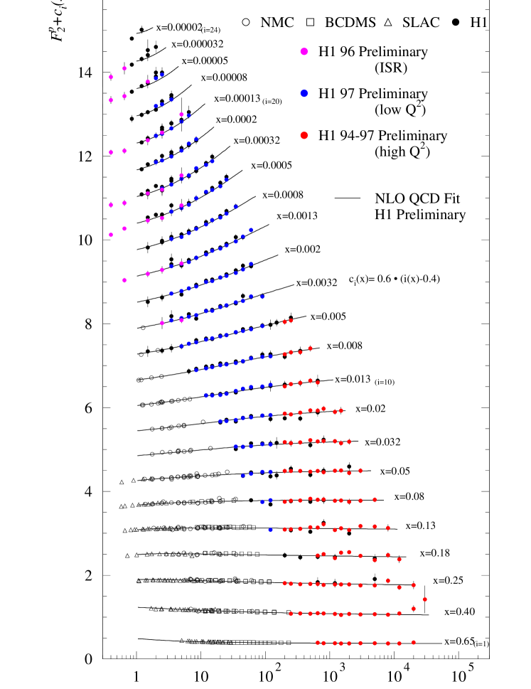
Figure 1: Next-to-leading order QCD fit to HERA and pre-HERA data on the proton structure function $F_{2}(x,Q^{2})$ [9].

Here we review this problem and propose a procedure to construct a meaningful improvement of the singlet splitting function at small $x$, using the information from the BFKL function. After recalling some basic notions we start by defining an alternative expansion for the BFKL function $\chi(M)$ which, unlike the usual expansion, is well behaved and stable when going from LO to NLO, at least for values far from $M=1$. This is obtained by adding suitable sequences of terms of the form $(\alpha_{s}/M)^{n}$ or $\alpha_{s}(\alpha_{s}/M)^{n}$ to $\alpha_{s}\chi_{0}$ or $\alpha_{s}^{2}\chi_{1}$ respectively. The coefficients are determined by the known form of the singlet anomalous dimension at one and two loops. This amounts to a resummation [18] of $(\alpha_{s}\log{Q^{2}/\mu^{2}})^{n}$ terms in the inverse $M$-Mellin transform space. This way of improving $\chi$ is completely analogous to the usual way of improving $\gamma$ [20]. One important point, which is naturally reproduced with good accuracy by the above procedure, is the observation that the value of $\chi(M)$ at $M=0$ is fixed by momentum conservation to be $\chi(0)=1$. This observation plays a crucial role in formulating the novel expansion and explains why the normal BFKL expansion is so unstable near $M=0$, with $\chi_{0}\sim 1/M$, $\chi_{1}\sim-1/M^{2}$ and so on. This rather model–independent step is already sufficient to show that no catastrophic deviations from the NLO approximation of the evolution equations are to be expected. The next step is to use this novel expansion of $\chi$ to determine small $x$ resummation corrections to add to the LO and NLO anomalous dimensions $\gamma$. Defining $\lambda$ as the minimum value of $\chi$, $\chi(M_{min})=\lambda$, and using the results of ref. [21], a meaningful expansion for the improved anomalous dimension is written down in terms of $\chi_{0}$, $\chi_{1}$, and $\lambda$. The large negative correction to $\lambda_{0}/\alpha_{s}=\chi_{0}(1/2)$ induced by $\alpha_{s}\chi_{1}$, that is formally of order $\alpha_{s}$ but actually is of order one for the relevant values of $\alpha_{s}$, suggests that $\lambda$ should be reinterpreted as a nonperturbative parameter. We conclude by showing that the very good agreement of the data with the NLO evolution equation can be obtained by choosing a small value of $\lambda$, compatible with zero.

2 $Q^{2}$ Evolution at Small $x$

The behaviour of structure functions at small $x$ is dominated by the singlet parton component. Thus we consider the singlet parton density

$$G(\xi,t)=x[g(x,Q^{2})+k_{q}\otimes q(x,Q^{2})],$$ (1)

where $\xi=\log{1/x}$, $t=\log{Q^{2}/\mu^{2}}$, $g(x,Q^{2})$ and $q(x,Q^{2})$ are the gluon and singlet quark parton densities, respectively, and $k_{q}$ is such that, for each moment

$$G(N,t)=\int^{\infty}_{0}\!d\xi\,e^{-N\xi}~{}G(\xi,t),$$ (2)

the associated anomalous dimension $\gamma(N,\alpha_{s}(t))$ corresponds to the largest eigenvalue in the singlet sector. At large $t$ and fixed $\xi$ the evolution equation in $N$-moment space is then

$${{d}\over{dt}}G(N,t)=\gamma(N,\alpha_{s}(t))~{}G(N,t),$$ (3)

where $\alpha_{s}(t)$ is the running coupling. The anomalous dimension is completely known at one and two loop level:

$$\gamma(N,\alpha_{s})=\alpha_{s}\gamma_{0}(N)+\alpha_{s}^{2}\gamma_{1}(N)+\dots\>.$$ (4)

As $\gamma(N,\alpha_{s})$ is, for each $N$, the largest eigenvalue in the singlet sector, momentum conservation order by order in $\alpha_{s}$ implies that

$$\gamma(1,\alpha_{s})=\gamma_{0}(1)=\gamma_{1}(1)=...=0.$$ (5)

The solution of eq.(3) is given by

$$G(N,t)=G(N,0)~{}\exp{\int^{\alpha_{s}(t)}_{\alpha_{s}}~{}d\alpha_{s}^{\prime}~{}{{\gamma(N,\alpha_{s}^{\prime})}\over{\beta(\alpha_{s}^{\prime})}}}$$ (6)

where $\alpha_{s}\equiv\alpha_{s}(0)$ and the QCD beta function $\beta(\alpha_{s})$ is defined by

$${{d\alpha_{s}(t)}\over{dt}}=\beta(\alpha_{s}(t));~{}~{}~{}~{}~{}\beta(\alpha_{s})=-b\alpha_{s}^{2}(1+b^{\prime}\alpha_{s}+.....);~{}~{}~{}~{}~{}b={{\beta_{0}}\over{4\pi}}={{11n_{c}-2n_{f}}\over{12\pi}}$$ (7)

At one loop accuracy $\gamma(N,\alpha_{s})=\alpha_{s}\gamma_{0}(N)$ and the solution reduces to:

$$G(N,t)=G(N,0)~{}e^{(\gamma_{0}\eta/b)}=G(N,0)~{}[{{\alpha_{s}}\over{\alpha_{s}(t)}}]^{\gamma_{0}/b};~{}~{}~{}~{}\eta=\log{{{\alpha_{s}}\over{\alpha_{s}(t)}}}$$ (8)

Of formal interest is the solution in the limit of fixed coupling. In general, in this limit, we have $G(N,t)=G(N,0)~{}\exp{[\gamma(N,\alpha_{s})t]}$ and, at one loop, $G(N,t)=G(N,0)~{}\exp{(\gamma_{0}\alpha_{s}t)}$. Comparing with the running coupling case at one loop, we see that $\alpha_{s}t$ at fixed coupling is replaced by $\eta/b$ at running coupling. In fact by expanding we have

$$\eta=\log{{{\alpha_{s}}\over{\alpha_{s}(t)}}}=\log{(1+b\alpha_{s}t)}=b\alpha_{s}t+......$$ (9)

It is useful to keep in mind this translation rule for one loop results.

We now consider the small $x$ behaviour of the one loop solution. Small $x$ means large $\xi$, hence small $N$. At small $N$, $\gamma_{0}(N)={{n_{c}}\over{\pi N}}+\ldots$. The $1/N$ behaviour correspond to the $1/x$ behaviour of the one loop singlet splitting function $P_{0}(x)$, the Mellin transform of $\gamma_{0}$: $\gamma(N)=\int^{1}_{0}\!dx\,x^{N}\!P(x)$. In general $P(x)\sim 1/x(\log(1/x))^{n}$ corresponds to $\gamma(N)\sim n!/N^{n+1}$. We can add a constant term to $\gamma_{0}(N)$ in such a way that the momentum conservation condition at $N=1$ is respected:

$$\gamma_{0}(N)\approx{{n_{c}}\over{\pi}}({{1}\over{N}}-1)+.....$$ (10)

This addition provides a good approximation in a wide region extending from $N\sim 0$ up to $N\sim 1$. From eq.(8) one obtains the leading behaviour:

$$G(N,t)=G(N,0)~{}\exp\left[{{n_{c}}\over{\pi}}{{\eta}\over{b}}({{1}\over{N}}-1)\right]$$ (11)

By taking the inverse Mellin transform we obtain:

$$G(\xi,t)=\int_{c-i\infty}^{c+i\infty}\!{{dN}\over{2\pi i}}\!\exp{(N\xi+{{n_{c}\eta}\over{\pi b}}({{1}\over{N}}-1))}G(N,0)$$ (12)

where the integral is along the imaginary axis at $RealN=c$. The leading behaviour at small $x$ is obtained by the saddle point method (see Appendix). Let $N_{0}$ be the point where the derivative of the exponent vanishes:

$${{d}\over{dN}}\left(N\xi+{{n_{c}\eta}\over{\pi b}}\left({{1}\over{N}}-1\right)\right)_{N=N_{0}}=0,~{}~{}~{}~{}N_{0}=\sqrt{{{n_{c}\eta}\over{\pi b\xi}}}$$ (13)

At $N_{0}$ the value of the exponent is:

$$\left(N\xi+{{n_{c}\eta}\over{\pi b}}\left({{1}\over{N}}-1\right)\right)_{N=N_{0}}=\sqrt{{{4n_{c}\eta\xi}\over{\pi b}}}-{{n_{c}\eta}\over{\pi b}}$$ (14)

For $G(N,0)$ regular at $N\geq 0$, the resulting small $x$ behaviour is given by:

$$G(\xi,t)=G(N_{0},0)\eta^{\hbox{${{1}\over{4}}$}}\xi^{-\hbox{${{3}\over{4}}$}}\exp{\sqrt{{{4n_{c}\eta\xi}\over{\pi b}}}}\exp{(-{{n_{c}\eta}\over{\pi b}})}$$ (15)

This is the well known ”double scaling” behaviour, first predicted in ref.[7] and developed in refs.[8]. The exponential factor

$$\exp{\sqrt{{{4n_{c}\eta\xi}\over{\pi b}}}}\approx\exp{\sqrt{{{4n_{c}}\over{\pi b}}\log{{{1}\over{x}}}\log{{{\log{Q^{2}/\Lambda^{2}}}\over{\log{\mu^{2}/\Lambda^{2}}}}}}}$$ (16)

produces a peak at small $x$ which increases with $Q^{2}$. The $x$ behaviour is weaker than any power of $x$ but stronger than any power of a logarithm. This one loop prediction is not much modified by NLO corrections because the computed two loop anomalous dimension $\gamma_{1}(N)$ also behaves like $1/N$. And in fact the complete NLO QCD evolution reproduces the double scaling exponential rise quite accurately. As already mentioned the HERA data are quite well fitted for $Q^{2}\geq~{}1-4~{}{\rm GeV}^{2}$ by QCD $Q^{2}$ evolution computed at NLO accuracy. This agreement of the data with the usual evolution equations is however rather unexpected. In fact the $Q^{2}$ evolution takes into account all terms of order $[\alpha_{s}\log{1/x}\log{Q^{2}}]^{n}$ and $[\alpha_{s}\log{Q^{2}}]^{n}$ and are valid for sufficiently large $Q^{2}$ and $x$ small but fixed. However possible terms of order $[\alpha_{s}\log{1/x}]^{n}$ are not included in the splitting function, so that the results are not necessarily reliable for sufficiently small $x$ at fixed $Q^{2}$. The powerful approach based on the BFKL equation provides a suitable tool towards an estimate of these terms and will now be discussed.

3 The BFKL Function

The starting point of the BFKL theory is that, at large $\xi$ and fixed $Q^{2}$ (in particular at fixed $\alpha_{s}$), the following $x$ evolution equation for $M$ moments was proven valid:

$${{d}\over{d\xi}}G(\xi,M)=\chi(M,\alpha_{s})~{}G(\xi,M),$$ (17)

where

$$G(\xi,M)=\int^{\infty}_{-\infty}\!dt\,e^{-Mt}~{}G(\xi,t),$$ (18)

For convergence, we consider $0<M<1$ as the physical region and assume that $G(\xi,t)$ vanishes as $Q^{2}$ in the photoproduction limit $Q^{2}\rightarrow\!0$ and approaches a constant modulo logs in the limit of large $Q^{2}$. In eq.(17) $\chi(M,\alpha_{s})$ is the BFKL function which is now known at NLO accuracy:

$$\chi(M,\alpha_{s})=\alpha_{s}\chi_{0}(M)+\alpha_{s}^{2}\chi_{1}(M)+\dots\>.$$ (19)

The BFKL function has been computed in perturbation theory at one and two loops starting from the large $s$ behaviour of the amplitude for gluon-gluon scattering.

We consider $T$, the absorptive part of the $A+B\rightarrow A+B$ forward scattering amplitude from gluon exchange, as depicted in fig. 2. $A$ and $B$ are generic real or virtual particles. In the case of interest, $A$ will be the virtual photon and $B$ the proton. From the optical theorem $T$ is proportional to the total $A+B$ cross section $\sigma$. We are interested in the gluon exchange component which is dominant in the singlet sector. So in the deep inelastic scattering case the virtual photon $A$ is attached to a quark loop which is included in $\phi_{A}$. Going down vertically then there is the g-g amplitude $\Gamma_{N}$ and finally the proton blob $\phi_{B}$. The cross section $\sigma$ can be written as:

$$\sigma\sim\int\!{{d^{2}k_{1}}\over{k_{1}^{2}}}\!\phi_{A}(\vec{k}_{1})\int\!{{d^{2}k_{2}}\over{k_{2}^{2}}}\!\phi_{B}(\vec{k}_{2})\int_{a-i\infty}^{a+i\infty}\!{{dN}\over{2\pi i}}~{}({{s}\over{k_{1}k_{2}}})^{N}~{}\Gamma_{N}(\vec{k}_{1},\vec{k}_{2})$$ (20)

Here $k_{1,2}$ are transverse momentum vectors of the s-channel gluons with virtuality $-(\vec{k})^{2}$, $\phi_{A,B}$ are suitable hadronic structure functions, $\Gamma_{N}$ is the $g$-$g$ kernel and $s=2p_{A}p_{B}$ is the squared invariant mass of the colliding particles. Note that a symmetric scale choice was adopted in the $s$ factor. The $g$-$g$ kernel in the $\overline{\rm MS}$ scheme obeys the generalised BFKL equation:

$$N\Gamma_{N}(\vec{k}_{1},\vec{k}_{2})=\delta^{(2)}(\vec{k}_{1}-\vec{k}_{2})+\int\!d^{2}k~{}K(\vec{k}_{1},\vec{k})~{}\Gamma_{N}(\vec{k},\vec{k}_{2})$$ (21)

The BFKL equation can be cast in the form of the $x$ evolution equation (17) inverting the $N$-Mellin transform eq. (2) and taking an $M$-Mellin transform eq. (18). The inversion of the $N$-Mellin turns multiplication by $N$ into differentiation with respect to $\ln(1/x)$, and the $M$-Mellin turns the convolution with respect to $k^{2}$ into an ordinary product. It then follows that the $\chi(M,\alpha_{s})$ function is related to $K$ by $M$-Mellin transformation:

$$\chi(M,\alpha_{s})=\int\!d^{2}k~{}K(\vec{k}_{1},\vec{k})~{}({{k^{2}}\over{k_{1}^{2}}})^{M-1}$$ (22)

At NLO and beyond, $\chi(M,\alpha_{s})$ can acquire a further dependence on $k_{1}^{2}$ due to the running of the coupling. From the symmetry under $\vec{k}_{1}\rightarrow\vec{k}_{2}$ exchange of $\Gamma_{N}$, the symmetry of $K$ also follows and in turn, at leading order, this implies that $\chi_{0}(M)=\chi_{0}(1-M)$. We have slightly cheated in this derivation in that the variable $N$ in eq. (21) is defined by the moment integration of eq. (20), i.e. with the symmetric factor $({{s}\over{k_{1}k_{2}}})^{N}$. The $N$ moments eq. (2) instead are taken with the factor $x^{N}=({{s}\over{Q^{2}}})^{-N}$ where $Q^{2}$ is the virtuality of one of the two particles, say $Q^{2}=k_{1}^{2}$. This difference is irrelevant at LO, but at NLO it must be taken into account and modifies [14] the relation between $\chi$ and $K$ eq. (22).

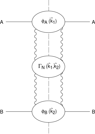
Figure 2: The process $A+B\rightarrow A+B$.

At one loop accuracy $\chi_{0}(M)$ is scheme and scale independent and has the following simple form (see fig.4 below):

$$\chi_{0}(M)={{n_{c}}\over{\pi}}\int_{0}^{1}~{}{{dz}\over{1-z}}~{}[z^{M-1}+z^{-M}-2]$$ (23)

(an alternative expression is $\chi_{0}(M)=n_{c}/\pi[2\psi(1)-\psi(M)-\psi(1-M)]$ with $\psi(M)=\Gamma^{\prime}(M)/\Gamma(M)$, where $\Gamma$ is the Euler gamma function). By expanding the denominator and performing the integration, one finds the expression:

$$\chi_{0}(M)={{n_{c}}\over{\pi}}\sum_{n=0}^{\infty}[{{1}\over{M+n}}+{{1}\over{n+1-M}}-{{2}\over{n+1}}]={{1}\over{M}}+2\zeta(3)M^{2}+2\zeta(5)M^{4}+.....$$ (24)

Also note that

$$\chi_{0}(\hbox{${{1}\over{2}}$})={{n_{c}}\over{\pi}}4\ln{2}$$ (25)

In eq. (17) the coupling $\alpha_{s}$ is fixed. The inclusion of running effects in the BFKL theory is a delicate point. If we are only interested to next-to-leading log $1/x$ accuracy, the running of the coupling in the evolution equation (3) can be expanded out to leading order in $t$: $\alpha_{s}(t)=\alpha_{s}(\mu^{2})(1-b\alpha_{s}(\mu^{2})t)$. Upon $M$-mellin transformation, this corresponds to a differential operator: $\alpha_{s}(M)=\alpha_{s}(1+b\alpha_{s}{d\over dM})$, which can be used in the $x$ evolution equation (17). This affects the relation between the $t$ and $x$ evolution equations, and in particular it modifies the relations between $\chi$ and the anomalous dimension $\gamma$ which we will derive in the next section (duality relation). However, for all practical purposes, this modification can be simply viewed as the result of an additional contribution to $\chi$: once this contribution is incorporated in $\chi$, the anomalous dimension $\gamma$ is given by the duality relation given in the next session. Henceforth, we assume that $\chi$ includes such contribution, at the appropriate order in the small $x$ expansion. To next-to-leading order in $\alpha_{s}$ (i.e. to NLLx), this corresponds to a contribution to $\chi_{1}$ proportional to the first coefficient $\beta_{0}=\hbox{${{11}\over{3}}$}n_{c}-\hbox{${{2}\over{3}}$}n_{f}$ of the $\beta$-function. Since the extra term depends on the definition of the gluon density, it is also necessary to specify the choice of factorization scheme: here we choose the $\overline{\rm MS}$ scheme, so that the $\chi_{1}$ that we will consider in the sequel is given by [21]

$$\chi_{1}(M)=\hbox{${{1}\over{4\pi^{2}}}$}n_{c}^{2}\tilde{\delta}(M)+\hbox{${{1}\over{8\pi^{2}}}$}\beta_{0}n_{c}((2\psi^{\prime}(1)-\psi^{\prime}(M)-\psi^{\prime}(1-M))+\hbox{${{1}\over{4n_{c}^{2}}}$}\chi_{0}(M)^{2},$$ (26)

where the function $\tilde{\delta}$ is defined in the first of ref. [14]. Note that beyond the leading order the symmetry of the BFKL function under $M\rightarrow 1-M$ is destroyed by the effects of running and by the fact that the scales $k_{1}$ and $k_{2}$ are very different in the actual case of interest. As a result the actual BFKL function which is relevant for deep inelastic leptoproduction is not perturbative near $M=1$, the point where the soft scale is approached.

To start exploring the physical significance of the $x$ evolution equation, we work in the fixed coupling approximation. The solution of eq.(17) is given by:

$$G(\xi,M)=G(0,M)\!\exp{\left[\chi(M,\alpha_{s})\xi\right]}$$ (27)

By taking the inverse Mellin transform, we obtain:

$$G(\xi,t)=\int_{c-i\infty}^{c+i\infty}\!{{dM}\over{2\pi i}}\!\exp{[Mt+\chi(M,\alpha_{s})\xi]}G(0,M)$$ (28)

For $t$ and $\xi$ large we consider the saddle point condition (for simplicity, we restrict our discussion to the LO):

$${{d}\over{dM}}\bigg{(}Mt+\alpha_{s}\chi_{0}(M)\xi\bigg{)}_{M=M_{0}}=0,~{}~{}~{}~{}\rm{or}~{}~{}~{}~{}{{t}\over{\xi}}=-\alpha_{s}\chi^{\prime}_{0}(M_{0})$$ (29)

With $t$ and $\xi$ both large we can study three different interesting limits: 1) $t/\xi$ large and positive (i.e. the limit $Q^{2}\rightarrow\infty$, $\xi$ large but fixed); 2) $t/\xi\rightarrow 0$ (or the Regge limit: $x\rightarrow 0$ and $Q^{2}$ large but fixed); 3) $t/\xi\rightarrow-\infty$ (or the photoproduction limit: $Q^{2}\rightarrow 0$ and $\xi$ large but fixed). In case 1) at $M_{0}$ the derivative must be large and negative, thus $M_{0}$ is small (see fig. 4). One finds:

$$M_{0}=\sqrt{{{n_{c}\alpha_{s}\xi}\over{\pi t}}},~{}~{}~{}~{}~{}~{}~{}G(\xi,t)\propto\exp{[M_{0}t+\alpha_{s}\chi_{0}(M_{0})\xi]}\approx\exp{\sqrt{{{4n_{c}\alpha_{s}t\xi}\over{\pi}}}}$$ (30)

Since we know that $\alpha_{s}t$ at fixed $\alpha_{s}$ corresponds to $\eta/b$ for running $\alpha_{s}$, we see that the double scaling result, eq.(15), is reproduced. In case 2), $t/\xi\rightarrow 0$ and the derivative must vanish at $M_{0}$, or $M_{0}=1/2$. The asymptotic behaviour is fixed by $\chi_{0}(1/2)$ (see eq.(25)) and we have:

$$G(\xi,t)\propto\exp{[\alpha_{s}\chi_{0}(1/2)\xi]}\approx x^{-\lambda_{0}},~{}~{}~{}~{}~{}~{}\lambda_{0}=\alpha_{s}{{n_{c}}\over{\pi}}4\ln{2}$$ (31)

This is the hard Pomeron prediction (as opposed to the soft Pomeron, or $\lambda_{0}\approx 0$),which is well known but of dubious physical relevance, as we shall see in the following. In case 3) $t/\xi$ is large and negative, so the derivative must be large and positive, which leads to $M_{0}\approx 1$ where $\chi_{0}(M)\approx n_{c}/[\pi(1-M)]$. A simple calculation leads to:

$$M_{0}=1-\sqrt{{{n_{c}\alpha_{s}\xi}\over{\pi|t|}}},~{}~{}~{}~{}~{}~{}G(\xi,t)\propto Q^{2}\exp{\sqrt{{{4n_{c}\xi\alpha_{s}|t|}\over{\pi}}}}$$ (32)

This result is qualitatively encouraging, because it leads to the correct linear vanishing of $G(\xi,t)$ in $Q^{2}$ in the photoproduction limit [23]. But, quantitatively we cannot trust this result, because non perturbative effects must be important at $Q^{2}\approx 0$. Actually this confirms that the BFKL function must contain non perturbative effects near $M=1$ otherwise photoproduction would also be perturbative.

4 The Duality Relations

In the region where $Q^{2}$ and $1/x$ are both large the $t$ and $\xi$ evolution equations, i.e. eqs.(3,17), are simultaneously valid, and their mutual consistency requires the validity of the “duality” relation [12, 23]:

$$\chi(\gamma(N,\alpha_{s}),\alpha_{s})=N,$$ (33)

and its inverse

$$\gamma(\chi(M,\alpha_{s}),\alpha_{s})=M.$$ (34)

In order to derive the duality relations we start from the $x$ evolution equation, eq.(17), and take the $x$ Mellin transform of both sides:

$$\int^{\infty}_{0}~{}d\xi~{}e^{-N\xi}~{}{{d}\over{d\xi}}~{}G(\xi,M)=\chi(M,\alpha_{s})~{}G(N,M)$$ (35)

Integration by parts leads to:

$$[e^{-N\xi}~{}G(\xi,M)]^{\infty}_{0}+NG(N,M)=\chi(M,\alpha_{s})~{}G(N,M)$$ (36)

The square bracket on the l.h.s is determined by $\xi\sim 0$ and provides an N independent boundary condition, which we denote by $-H_{0}(M)$ (recall that the $x$ evolution equation is only valid at large $\xi$). Solving for $G(N,M)$, we find:

$$G(N,M)={{H_{0}(M)}\over{N-\chi(M,\alpha_{s})}}$$ (37)

The position of the singularity in $N$ fixes the large $t$ behaviour of $G(N,t)$:

$$G(N,t)=\int_{c-i\infty}^{c+i\infty}\!{{dM}\over{2\pi i}}~{}\exp{Mt}~{}G(N,M)\mathrel{\mathop{\sim}\limits_{\scriptscriptstyle{t\rightarrow\infty}}}\chi(M_{p},\alpha_{s})=N$$ (38)

while the contribution of additional singularities further on the left of $M_{p}$ is suppressed by powers of $Q^{2}$. Then, at fixed $\alpha_{s}$, this must coincide with

$$G(N,t)\mathrel{\mathop{\sim}\limits_{\scriptscriptstyle{t\rightarrow\infty}}}e^{\gamma(N,\alpha_{s})t}$$ (39)

where $\gamma$ is the anomalous dimension function at all order in $\alpha_{s}$. Thus $M_{p}=\gamma(N,\alpha_{s})$ and the duality relation eq.(33), and its inverse, eq.(34), are obtained. These relations are true for the complete leading twist contribution in the domain where the $t$ and $\xi$ evolution equations, i.e. eqs.(3,17), are simultaneously valid.

                 

Figure 3: Graphical representation of different expansions of (a) $\gamma$ and (b) $\chi$ in powers of $\alpha_{s}$ and $1/N$ (a) and $1/M$ (b) to order $m$ and $n$ respectively, and the different relations between these expansions. Vertical lines correspond to terms of the same fixed order in $\alpha_{s}$: for example the one loop anomalous dimension $\gamma_{0}$ contains terms with $m=1$, $n=1,0,-1,-2,\ldots$. Diagonal lines correspond to terms of the same order in $\alpha_{s}$ at fixed $\alpha_{s}\over N$ (a) or $\alpha_{s}\over M$ (b): for example $\gamma_{s}(\alpha_{s}/N)$ contains terms with $m=n=1,2,3,\ldots$. The sum of terms in a vertical line of the $\gamma$ plot is related by duality eqs. (33,34) to the sum of terms in a diagonal line in the $\chi$ plot and conversely (marked by the same line style). The solid lines denote terms of the same order in the “envelope” or “double leading” expansion discussed in the text.

Using eq. (33), knowledge of the expansion eq. (19) of $\chi(M,\alpha_{s})$ to LO and NLO in $\alpha_{s}$ at fixed $M$ determines the coefficients of the expansion of $\gamma(N,\alpha_{s})$ in powers of $\alpha_{s}$ at fixed ${{\alpha_{s}}\over{N}}$:

$$\gamma(N,\alpha_{s})=\gamma_{s}(\hbox{${{\alpha_{s}}\over{N}}$})+\alpha_{s}\gamma_{ss}(\hbox{${{\alpha_{s}}\over{N}}$})+\ldots,$$ (40)

where $\gamma_{s}$ and $\gamma_{ss}$ contain respectively sums of all the leading and subleading singularities of $\gamma$ (see fig. 3). To derive the expressions of $\gamma_{s}$ and $\gamma_{ss}$ we start from eq.(33) written in the form:

$$\alpha_{s}\chi_{0}[\gamma_{s}(\hbox{${{\alpha_{s}}\over{N}}$})+\alpha_{s}\gamma_{ss}(\hbox{${{\alpha_{s}}\over{N}}$})+...]+\alpha_{s}^{2}\chi_{1}[\gamma_{s}(\hbox{${{\alpha_{s}}\over{N}}$})+...]+....=N$$ (41)

We then expand in $\alpha_{s}$ at $\alpha_{s}/N$ fixed:

$$\chi_{0}(\gamma_{s}(\hbox{${{\alpha_{s}}\over{N}}$}))+\alpha_{s}\chi^{\prime}_{0}(\gamma_{s}(\hbox{${{\alpha_{s}}\over{N}}$}))~{}\gamma_{ss}(\hbox{${{\alpha_{s}}\over{N}}$})+\alpha_{s}\chi_{1}(\gamma_{s}(\hbox{${{\alpha_{s}}\over{N}}$}))+....={{N}\over{\alpha_{s}}}$$ (42)

From this we find the relations:

$$\chi_{0}(\gamma_{s}(\hbox{${{\alpha_{s}}\over{N}}$})) = {N\over\alpha_{s}},$$ (43)

$$\gamma_{ss}(\hbox{${{\alpha_{s}}\over{N}}$}) = -{{\chi_{1}(\gamma_{s}(\hbox{${{\alpha_{s}}\over{N}}$}))}\over{\chi^{\prime}_{0}(\gamma_{s}(\hbox{${{\alpha_{s}}\over{N}}$}))}}.$$ (44)

This corresponds to an expansion of the splitting function in logarithms of $x$: if for example we write

$$\gamma_{s}({{\alpha_{s}}\over{N}})=\sum_{k=1}^{\infty}g_{k}^{(s)}\left({{\alpha_{s}}\over{N}}\right)^{k}$$ (45)

then the associated splitting function is given by

$$P_{s}(\alpha_{s}\xi)\equiv\int_{c-i\infty}^{c+i\infty}\!{{dN}\over{2\pi i\alpha_{s}}}\,e^{N\xi}\,\gamma_{s}(\hbox{${{\alpha_{s}}\over{N}}$})=\sum_{k=1}^{\infty}{{g_{k}^{(s)}}\over{(k-1)!}}(\alpha_{s}\xi)^{(k-1)},$$ (46)

and similarly for the subleading singularities $P_{ss}(\alpha_{s}\xi)$, etc. From eq.(24) it follows that

$$g_{1}^{(s)}=n_{c}/\pi,\>g_{2}^{(s)}=g_{3}^{(s)}=0\>,g_{4}^{(s)}=2\zeta(3)n_{c}/\pi,\dots$$ (47)

We see that the logaritmic terms in $P_{s}$ only start at order $\alpha_{s}^{3}$ due to the vanishing of $g_{2}^{(s)}$ and $g_{3}^{(s)}$. It is also important to observe that the coefficients of the $P_{s}$ expansion are factorially suppressed with respect to those of $\gamma_{s}$. This implies that while the convergence radius of the $\gamma_{s}$ expansion is finite, that of $P_{s}$ is infinite.

At this point it is interesting to make a digression and compare the small $x$ behaviour of the singlet structure functions in the spacelike region with that of singlet fragmentation functions in the timelike region. In the leading log approximation the timelike splitting functions, relevant for the evolution of fragmentation functions, are the same as the spacelike splitting functions. Therefore the solution to the one loop evolution equation in the small $x$ region is valid both for parton distributions in the spacelike region and for fragmentation functions in the timelike region. But if this were the correct asymptotic result at $x\rightarrow 0$ for the singlet framentation functions it would imply that the average multiplicity (the $N=0$ moment) is singular. Indeed it is in fact known [19] that, in the timelike region, the behaviour of the anomalous dimension near $N=0$ is actually modified by higher order terms according to:

$$\gamma(N,\alpha_{s})={{\alpha_{s}n_{c}}\over{\pi N}}-2({{\alpha_{s}n_{c}}\over{\pi}})^{2}{{1}\over{N^{3}}}+......={{1}\over{4}}[-N+\sqrt{N^{2}+{{8\alpha_{s}n_{c}}\over{\pi}}}]$$ (48)

In $x$ space this is equivalent to the occurrence of terms of order $\alpha_{s}[\alpha_{s}\log^{2}{1/x}]^{n-1}$ in nth order perturbation theory in $\alpha_{s}$. Thus there are two powers of log for each $\alpha_{s}$ in the timelike region instead than one. These terms modify the behaviour of $\gamma(N,\alpha_{s})$ near $N=0$ into a non singular one. This corresponds to the well known behaviour of the average multiplicity in gluon jets given by:

$$<n_{g}>\propto~{}\exp{\int_{\alpha_{s}}^{\alpha_{s}(t)}~{}d\alpha_{s}~{}{{\gamma(0,\alpha_{s})}\over{\beta(as)}}}\approx\exp{\sqrt{{{2n_{c}\log{Q^{2}/\Lambda^{2}}}\over{\pi b\log{\mu^{2}/\Lambda^{2}}}}}}$$ (49)

which is well supported by experiment. How is it possible that there is such a difference between the spacelike and timelike regions? That the fragmentation functions are more singular than the structure functions is due to the fact that in leptoproduction the final state is totally inclusive. Instead, when we compute the fragmentation of a gluon into a gluon, we fix the momentum of the observed soft gluon and so its associated infrared singularity cannot be canceled against the corresponding virtual contribution and appears in the result as an extra power of $\xi$.

Going back to the duality relations, the inverse duality eq. (34) relates the fixed order expansion eq. (4) of $\gamma(N,\alpha_{s})$ to an expansion of $\chi(M,\alpha_{s})$ in powers of $\alpha_{s}$ with ${{\alpha_{s}}\over{M}}$ fixed: if

$$\chi(M,\alpha_{s})=\chi_{s}(\hbox{${{\alpha_{s}}\over{M}}$})+\alpha_{s}\chi_{ss}(\hbox{${{\alpha_{s}}\over{M}}$})+\ldots,$$ (50)

where now $\chi_{s}(\hbox{${{\alpha_{s}}\over{M}}$})$ and $\chi_{ss}(\hbox{${{\alpha_{s}}\over{M}}$})$ contain the leading and subleading singularities respectively of $\chi(M,\alpha_{s})$, then

$$\gamma_{0}(\chi_{s}(\hbox{${{\alpha_{s}}\over{M}}$})) = {{M}\over{\alpha_{s}}},$$ (51)

$$\chi_{ss}(\hbox{${{\alpha_{s}}\over{M}}$}) = -{{\gamma_{1}(\chi_{s}(\hbox{${{\alpha_{s}}\over{M}}$}))}\over{\gamma^{\prime}_{0}(\chi_{s}(\hbox{${{\alpha_{s}}\over{M}}$}))}}.$$ (52)

We now discuss the physical implications of these formal results for the singlet splitting function at small $x$.

5 Improving the BFKL Expansion

In principle, since $\chi_{0}$ and $\chi_{1}$ are known, they can be used to construct an improvement of the splitting function which includes a summation of leading and subleading logarithms of $x$. However, as is now well known, the calculation [14, 15, 16] of $\chi_{1}$ has shown that this procedure is confronted with serious problems. The fixed order expansion eq. (19) is very badly behaved: at relevant values of $\alpha_{s}$ the NLO term completely overwhelms the LO term. In particular, near $M=0$, the behaviour is unstable, with $\chi_{0}\sim 1/M$, $\chi_{1}\sim-1/M^{2}$. Also, the value of $\chi$ near the minimum is subject to a large negative NLO correction, which turns the minimum into a maximum and can even reverse the sign of $\chi$ at the minimum: in $\overline{\rm MS}$ for $n_{f}=3$ or $4$, we approximately have

$$\chi(\hbox{${{1}\over{2}}$},\alpha_{s})\approx 2.65\alpha_{s}(1-6.2\alpha_{s}+...)$$ (53)

Finally, if one considers the resulting $\gamma_{s}$ and $\gamma_{ss}$ or their Mellin transforms $P_{s}(x)$ and $P_{ss}(x)$ one finds that the NLO terms become much larger than the LO terms and negative in the region of relevance for the HERA data [17]. We now discuss our proposals to deal with all these problems.

Our first observation is that a much more stable expansion for $\chi(M)$ can be obtained if we make appropriate use of the additional information which is contained in the one and two loop anomalous dimensions $\gamma_{0}$ and $\gamma_{1}$. Instead of trying to improve the fixed order expansion eq. (4) of $\gamma$ by all order summation of singularities deduced from the fixed order expansion eq. (19) of $\chi$, we attempt the converse: we improve $\chi_{0}(M)$ by adding to it the all order summation of singularities $\chi_{s}$ eq. (51) deduced from $\gamma_{0}$, $\chi_{1}(M)$ by adding to it $\chi_{ss}$ deduced from $\gamma_{1}$ eq. (52), and so on. It can then be seen that the instability at $M=0$ of the usual fixed order expansion of $\chi$ was inevitable: momentum conservation for the anomalous dimension, eq. (5), implies, given the duality relation, that the value of $\chi(M)$ at $M=0$ is fixed to unity, since from eq. (33) we see that at $N=1$

$$\chi(\gamma(1,\alpha_{s}),\alpha_{s})=\chi(0,\alpha_{s})=1.$$ (54)

It follows that the fixed order expansion of $\chi$ must be poorly behaved near $M=0$: a simple model of this behaviour is to think of replacing $\alpha_{s}/M$ with $\alpha_{s}/(M+\alpha_{s})=\alpha_{s}/M-\alpha_{s}^{2}/M^{2}+...$ in order to satisfy the momentum conservation constraint.

We thus propose a reorganization of the expansion of $\chi$ into a “double leading” (DL) expansion, organized in terms of “envelopes” of the contributions summarized in fig. 3b: each order contains a “vertical” sequence of terms of fixed order in $\alpha_{s}$, supplemented by a “diagonal” resummation of singular terms of the same order in $\alpha_{s}$ if $\alpha_{s}/M$ is considered fixed. To NLO the new expansion is thus

$$\chi(M,\alpha_{s}) =\left[\alpha_{s}\chi_{0}(M)+\chi_{s}\left({\hbox{${{\alpha_{s}}\over{M}}$}}\right)-\hbox{${{n_{c}\alpha_{s}}\over{\pi M}}$}\right]$$ (55)

$$\qquad+\alpha_{s}\left[\alpha_{s}\chi_{1}(M)+\chi_{ss}\left({\hbox{${{\alpha_{s}}\over{M}}$}}\right)-\alpha_{s}\left(\hbox{${{f_{2}}\over{M^{2}}}$}+\hbox{${{f_{1}}\over{M}}$}\right)-f_{0}\right]+\cdots$$

where the LO and NLO terms are contained in the respective square brackets. Thus the LO term contains three contributions: $\chi_{0}(M)$ is the leading BFKL function eq. (19), $\chi_{s}(\alpha_{s}/M)$ eq. (51) are resummed leading singularities deduced from the one loop anomalous dimension, and $n_{c}\alpha_{s}/(\pi M)$ is subtracted to avoid double counting. At LO the momentum conservation constraint eq. (54) is satisfied exactly because $\gamma_{0}(1)=0$ and $[\chi_{0}(M)-\hbox{${{n_{c}}\over{\pi M}}$}]\sim M^{2}$ near $M=0$ (see eq.(24)). At NLO there are again three types of contributions: $\chi_{1}(M)$ from the NLO fixed order calculation (eq. (26)), the resummed subleading singularities $\chi_{ss}(\alpha_{s}/M)$ deduced from the two loop anomalous dimension, and three double counting terms, $f_{0}=0$, $f_{1}=-n_{f}(13+10n_{c}^{2})/(36\pi^{2}n_{c}^{3})$ and $f_{2}=n_{c}^{2}(11+2n_{f}/n_{c}^{3})/(12\pi^{2})$ (corresponding to those terms with $(m,n)=(1,0),(2,1),(2,2)$ respectively in fig. 3b). Note that at the next-to-leading level the momentum conservation constraint is not exactly satisfied because the constant contribution to $\chi_{1}$ does not vanish in $\overline{\rm MS}$, even though it is numerically very small (see fig. 4). It could be made exactly zero by a refinement of the double counting subtraction but we leave further discussion of this point for later.

Figure 4: Plots of different approximations to the $\chi$ function discussed in the text: the BFKL leading and next-to-leading order functions eq. (19), $\alpha_{s}\chi_{0}$ and $\alpha_{s}\chi_{0}+\alpha_{s}^{2}\chi_{1}$ (dashed); the LO and NLO dual $\alpha_{s}\chi_{s}$ and $\alpha_{s}\chi_{s}+\alpha_{s}^{2}\chi_{ss}$ of the one and two loop anomalous dimensions (solid), and the double-leading functions at LO and NLO defined in eq. (55) (dotdashed). Note that the double-leading curves coincide with the resummed ones at small $M$, and with the fixed order ones at large $M$.

Plots of the various LO and NLO approximations to $\chi$ are shown in fig. 4. In this and other plots in this paper we take $\alpha_{s}=0.2$, which is a typical value in the HERA region, and the number of active flavours $n_{f}=4$. We see that, as discussed above, the usual fixed order expansion eq. (19) in terms of $\chi_{0}$ and $\chi_{1}$ is very unstable. However, the new expansion eq. (55) is stable up to $M\mathrel{\hbox to0.0pt{\raise 2.15277pt\hbox{$<$}\hss}{\lower 2.15277pt\hbox{$\sim$}}}0.3-0.4$. Furthermore, in this region, $\chi$ evaluated in the double leading expansion (55) is very close to the resummations of leading and subleading singularities eq. (50) obtained by duality eq. (51,52) from the one and two loop anomalous dimensions. This shows that in this region the dominant contribution to $\chi$, and thus to $\gamma$ , comes from the resummation of logarithms of $Q^{2}/\mu^{2}$ with $Q^{2}\gg\mu^{2}$.

Beyond $M\sim 0.4$, the size of the contributions from collinear singular and nonsingular terms becomes comparable (after all here $Q^{2}\sim\mu^{2}$), but the calculation of the latter (from the fixed expansion eq. (19)) has become unstable due to the influence of the singularities at $M=1$. No complete and reliable description of $\chi$ seems possible without some sort of stabilization of these singularities. However, since they correspond to infrared singularities of the BFKL kernel (specifically logarithms of $Q^{2}/\mu^{2}$ with $Q^{2}\ll\mu^{2}$) this would necessarily be model dependent. In particular, such a stabilization cannot be easily deduced from the resummation of the $M=0$ singularities: the original symmetry of the gluon–gluon amplitude at large $s$ is spoiled by running coupling effects and by unknown effects from the coefficient function through which it is related to the deep-inelastic structure functions, in a way which is very difficult to control near the photoproduction limit $M\to 1$. We thus prefer not to enter into this problem: rather we will discuss later a practical procedure to bypass it.

The results summarized in fig. 4 clearly illustrate the superiority of the new double leading expansion of $\chi$ over the fixed order expansion, and already indicate that the complete $\chi$ function could after all lead to only small departures from ordinary two loop evolution.

6 Improving the Splitting Function Expansion

Having constructed a more satisfactory expansion eq. (55) of the kernel $\chi$, we now derive from it an improved form of the anomalous dimension $\gamma$ to be used in the evolution eq. (3), in order to achieve a more complete description of scaling violations valid both at large and small $x$. In principle, this can be done by using the duality relation eq. (33), which simply gives the function $\gamma$ as the inverse of the function $\chi$. However, in order to derive an analytic expression for $\gamma(N,\alpha_{s})$ which also allows us to clarify the relation to previous attempts we start from the naive double-leading expansion of $\gamma$ [20] in which terms are organized into “envelopes” of the contributions summarized in fig. 3a in an analogous way to the double leading expansion (55) of $\chi$:

$$\gamma(N,\alpha_{s}) =\left[\alpha_{s}\gamma_{0}(N)+\gamma_{s}\left(\hbox{${{\alpha_{s}}\over{N}}$}\right)-\hbox{${{n_{c}\alpha_{s}}\over{\pi N}}$}\right]$$ (56)

$$\qquad+\alpha_{s}\left[\alpha_{s}\gamma_{1}(N)+\gamma_{ss}\left(\hbox{${{\alpha_{s}}\over{N}}$}\right)-\alpha_{s}\left(\hbox{${{e_{2}}\over{N^{2}}}$}+\hbox{${{e_{1}}\over{N}}$}\right)-e_{0}\right]+\cdots,$$

where now $e_{2}=g_{2}^{(s)}=0$, $e_{1}=g_{1}^{(ss)}=n_{f}n_{c}(5+13/(2n_{c}^{2}))/(18\pi^{2})$ and $e_{0}=-(\hbox{${{11}\over{2}}$}n_{c}^{3}+n_{f})/(6\pi n_{c}^{2})$. In this equation, the leading and subleading singularities $\gamma_{s}$ and $\gamma_{ss}$ are obtained using duality eq. (33) from $\chi_{0}$ and $\chi_{1}$, and summed up to give expressions which are exact at NLLx. These are then added to the usual one and two loop contributions, and the subtractions take care of the double counting of singular terms.

It can be shown that the dual of the double leading expansion of $\chi$ eq. (55) coincides with this double leading expansion of $\gamma$ eq. (56) order by order in perturbation theory, up to terms which are higher order in the sense of the double leading expansions. However, it is clear that these additional subleading terms must be numerically important. Indeed, it is well know that at small $N$ the anomalous dimension in the small-$x$ expansion eq. (40) is completely dominated by $\gamma_{ss}(\alpha_{s}/N)$ which grows very large and negative, leading to completely unphysical results in the HERA region [17]. It is clear that this perturbative instability will also be a problem in the double leading expansion eq. (56). On the other hand, we know from fig. 4 that the exact dual of $\chi$ in double leading expansion is stable, and not too far from the usual two loop result. The origin of this instability problem, and a suitable reorganization of the perturbative expansion which allows the resummation of the dominant part of the subleading terms have been discussed in ref. [21]. After this resummation, the resulting expression for $\gamma$ in double leading expansion will be very close to the exact dual of the corresponding expansion of $\chi$.

To understand this point we consider the asymptotic behaviour of $P_{s}$ and $P_{ss}$ at large $\xi$. Starting from the definition of the splitting function as the inverse Mellin transform of the anomalous dimension $\gamma$ as given in eq.(46), we have:

$$P_{s}(\alpha_{s}\xi)\equiv\int_{c-i\infty}^{c+i\infty}\!{{dN}\over{2\pi i\alpha_{s}}}\,e^{N\xi}\,\gamma_{s}(\hbox{${{\alpha_{s}}\over{N}}$})=-\int_{c-i\infty}^{c+i\infty}\!{{d\gamma_{s}}\over{2\pi i}}\,e^{\alpha_{s}\chi_{0}(\gamma_{s})\xi}\,\gamma_{s}\chi^{\prime}_{0}(\gamma_{s})$$ (57)

where we have used eq.(43) to change the integration variable according to $dN=\alpha_{s}\chi^{\prime}_{0}(\gamma_{s})d\gamma_{s}$. Similarly for $P_{ss}$, by using the form of $\gamma_{ss}$ given in eq.(44), we obtain:

$$P_{ss}(\alpha_{s}\xi)\equiv\int_{c-i\infty}^{c+i\infty}\!{{dN}\over{2\pi i\alpha_{s}}}\,e^{N\xi}\,\gamma_{ss}(\hbox{${{\alpha_{s}}\over{N}}$})=+\int_{c-i\infty}^{c+i\infty}\!{{d\gamma_{s}}\over{2\pi i}}\,e^{\alpha_{s}\chi_{0}(\gamma_{s})\xi}\,\chi_{1}(\gamma_{s})$$ (58)

The asymptotic behaviour of $P_{s}$ and $P_{ss}$ at large $\xi$ can now be obtained by applying the saddle point method. Remembering that the only real minimum of $\chi_{0}(\gamma_{s})$ in the range $0<\gamma_{s}<1$ is at $\gamma_{s}=\hbox{${{1}\over{2}}$}$, and expanding around the minimum according to

$$\gamma_{s}\chi^{\prime}_{0}(\gamma_{s})=\hbox{${{1}\over{2}}$}\chi^{{}^{\prime\prime}}_{0}(\hbox{${{1}\over{2}}$})(\gamma_{s}-\hbox{${{1}\over{2}}$})~{}+~{}\chi^{{}^{\prime\prime}}_{0}(\hbox{${{1}\over{2}}$})~{}(\gamma_{s}-\hbox{${{1}\over{2}}$})^{2}+....;~{}~{}~{}~{}~{}\chi_{1}(\gamma_{s})=\chi_{1}(\hbox{${{1}\over{2}}$})+....$$ (59)

one finds (see the formulae on the saddle point method in Appendix):

$$P_{s}(\alpha_{s}\xi)\mathrel{\mathop{\sim}\limits_{\scriptscriptstyle{\xi\rightarrow\infty}}}e^{\alpha_{s}\chi_{0}(\hbox{${{1}\over{2}}$})\xi}=x^{-\lambda_{0}};~{}~{}~{}~{}~{}{{P_{ss}}\over{P_{s}}}\mathrel{\mathop{\sim}\limits_{\scriptscriptstyle{\xi\rightarrow\infty}}}\alpha_{s}\chi_{1}(\hbox{${{1}\over{2}}$})\xi.$$ (60)

We see that at sufficiently small values of $x$ $P_{ss}$ overwhelms $P_{s}$ causing the perturbative expansion to become unstable. Actually this occurs at not so small values of $x$ because $\chi_{1}/\chi_{0}$ is so large.

On the basis of these results the procedure of ref. [21] can be interpreted in a simple way whenever the all-order “true” function $\chi(M,\alpha_{s})$ possesses a minimum at a real value of $M$, $M_{min}$, with $0<M_{min}<1$ (although the final result for the anomalous dimension will retain its validity even in the absence of such minimum). Using $\lambda$ to denote this minimum value of $\chi$,

$$\lambda\equiv\chi(M_{min},\alpha_{s})=\lambda_{0}+\Delta\lambda,\qquad\lambda_{0}\equiv\alpha_{s}\chi_{0}(\hbox{${1\over 2}$})=\hbox{${{4n_{c}}\over{\pi}}$}\alpha_{s}\ln 2.$$ (61)

The instability turns out to be due to the fact that higher order contributions to $\gamma$ must change the asymptotic small $x$ behaviour from $x^{-\lambda_{0}}$ to $x^{-\lambda}~{}=~{}x^{-\lambda_{0}}e^{\Delta\lambda\xi}~{}\approx~{}x^{-\lambda_{0}}[1+\Delta\lambda\xi+....]$, with $\Delta\lambda=\alpha_{s}^{2}\chi_{1}(\hbox{${1\over 2}$})+\cdots$.Having understood the source of the problem we can now cure it by a suitable resummation procedure. In terms of splitting functions the proposed resummed expansion is simply

$$xP(x,\alpha_{s}) = \alpha_{s}e^{\xi\Delta\lambda}[P_{s}(\alpha_{s}\xi)+\alpha_{s}\tilde{P}_{ss}(\alpha_{s}\xi)+\dots]$$ (62)

$$= \alpha_{s}e^{\xi\Delta\lambda}[P_{s}(\alpha_{s}\xi)+\alpha_{s}P_{ss}(\alpha_{s}\xi)-\xi\Delta\lambda P_{s}(\alpha_{s}\xi)+\dots].$$

The expansion is now stable [21], in the sense that it may be shown that $\tilde{P}_{ss}(\alpha_{s}\xi)/P_{s}(\alpha_{s}\xi)$ remains bounded as $\xi\to\infty$: subleading corrections will then be small provided only that $\alpha_{s}$ is sufficiently small. Equivalently, this procedure consists of absorbing the value of the correction to the value of $\chi$ at the minimum into the leading order term in the expansion of $\chi$:

$$\chi(M,\alpha_{s}) = \alpha_{s}\chi_{0}(M)+\alpha_{s}^{2}\chi_{1}(M)+\dots$$ (63)

$$= (\alpha_{s}\chi_{0}(M)+\Delta\lambda)+\alpha_{s}^{2}\tilde{\chi}_{1}(M)+\cdots,$$

where $\tilde{\chi}_{n}(M)\equiv\chi_{n}(M)-c_{n}$, with $c_{n}$ chosen so that $\tilde{\chi}_{n}(M)$ no longer leads to an $O(\alpha_{s}^{n})$ shift in the minimum. Since the position $M_{min}$ of the all-order minimum is not known, one must in practice expand it in powers of $\alpha_{s}$ around the leading order value $M=\hbox{${1\over 2}$}$, so at higher orders the expressions for the subtraction constants $c_{n}$ can become quite complicated functions of $\chi_{i}$ and their derivatives at $M=\hbox{${1\over 2}$}$ [21]. However at NLO we have simply $c_{1}=\chi_{1}(\hbox{${1\over 2}$})$, so $\Delta\lambda=\alpha_{s}^{2}\chi_{1}(\hbox{${1\over 2}$})+\cdots$.

The corresponding expansion of $\gamma$ in resummed leading and subleading singularities can also be obtained from the duality eqs.(43,44,…) by treating $\chi_{0}+\Delta\lambda$ as the LO contribution to $\chi$, and the subsequent terms $\tilde{\chi}_{i}$ as perturbative corrections to it. Of course, since the reorganization eq. (63) amounts to a reshuffling of perturbative orders, to any finite order the anomalous dimension obtained in this way will be equal to the old one up to formally subleading corrections. Explicitly, we find in place of the previous expansion in sums of singularities eq. (40) the resummed expansion

$$\gamma(N,\alpha_{s})=\gamma_{s}\left(\hbox{${{\alpha_{s}}\over{N-\Delta\lambda}}$}\right)+\alpha_{s}\tilde{\gamma}_{ss}\left(\hbox{${{\alpha_{s}}\over{N-\Delta\lambda}}$}\right)+\dots,$$ (64)

where

$$\tilde{\gamma}_{ss}\left(\hbox{${{\alpha_{s}}\over{N-\Delta\lambda}}$}\right)\equiv\gamma_{ss}\left(\hbox{${{\alpha_{s}}\over{N-\Delta\lambda}}$}\right)-{\chi_{1}(\hbox{${1\over 2}$})\over\chi^{\prime}_{0}\left(\gamma_{s}\left(\hbox{${{\alpha_{s}}\over{N-\Delta\lambda}}$}\right)\right)}.$$ (65)

The shift in the denominators from $N$ to $N-\Delta\lambda$ results from combining the exponential $e^{-N\xi}$ of the Mellin transform with the exponential $e^{\Delta\lambda\xi}$ factored out in eq.(62).

We can thus replace the unresummed singularities $\gamma_{s}$ and $\gamma_{ss}$ in eq. (56) with the resummed singularities eq. (64) to obtain a double leading expansion with stable small $x$ behaviour:

$$\gamma(N,\alpha_{s}) = \left[\alpha_{s}\gamma_{0}(N)+\gamma_{s}(\hbox{${{\alpha_{s}}\over{N-\Delta\lambda}}$})-\alpha_{s}\hbox{${{n_{c}}\over{\pi N}}$}\right]$$ (66)

$$+\alpha_{s}\left[\alpha_{s}\gamma_{1}(N)+\tilde{\gamma}_{ss}(\hbox{${{\alpha_{s}}\over{N-\Delta\lambda}}$})-\alpha_{s}(\hbox{${{e_{2}}\over{N^{2}}}$}+\hbox{${{e_{1}}\over{N}}$})-e_{0}\right]+\cdots.$$

Momentum conservation is violated by the resummation because $\gamma_{s}$ and $\gamma_{ss}$ and the subtraction terms do not vanish at $N=1$. It can be restored by simply adding to the constant $e_{0}$ a further series of constant terms beginning at $O(\alpha_{s}^{2})$: these are all formally subleading in the double leading expansion. This constant shift in $\gamma$ is precisely analogous to the shift made on $\chi$ in eq. (61) which generated the resummation.

It is important to recognize that there is inevitably an ambiguity in the double counting subtraction terms in eq. (66). For example, at the leading order of the double leading expansion instead of subtracting $n_{c}\alpha_{s}\over\pi N$ we could have subtracted $n_{c}\alpha_{s}\over\pi(N-\Delta\lambda)$, since this differs only by formally subleading terms: $\Delta\lambda=O(\alpha_{s}^{2})$, so

$${\alpha_{s}\over N}={\alpha_{s}\over N-\Delta\lambda}\left(1-{\Delta\lambda\over N-\Delta\lambda}+\dots\right).$$ (67)

Following the same type of subtraction at NLO, the resummed double leading anomalous dimension may thus be written as

$$\gamma(N,\alpha_{s}) = \left[\alpha_{s}\gamma_{0}(N)+\gamma_{s}(\hbox{${{\alpha_{s}}\over{N-\Delta\lambda}}$})-\alpha_{s}\hbox{${{n_{c}}\over{\pi(N-\Delta\lambda)}}$}\right]$$

$$\quad+\alpha_{s}\left[\alpha_{s}\gamma_{1}(N)+\tilde{\gamma}_{ss}(\hbox{${{\alpha_{s}}\over{N-\Delta\lambda}}$})+\hbox{${{n_{c}\Delta\lambda}\over{\pi(N-\Delta\lambda)^{2}}}$}\right.$$

$$\qquad\left.-\alpha_{s}(\hbox{${{e_{2}}\over{(N-\Delta\lambda)^{2}}}$}+\hbox{${{e_{1}}\over{N-\Delta\lambda}}$})-e_{0}\right]+\cdots,$$

where the new contribution proportional to $n_{c}\Delta\lambda$ in the NLO subtraction is due to the fact that to NLO accuracy we cannot simply replace $\alpha_{s}/N$ with $\alpha_{s}/(N-\Delta\lambda)$, but we must retain the NLO correction term in eq. (67). The characteristic feature of this alternative resummation is that the fixed order anomalous dimensions $\gamma_{0}$, $\gamma_{1}$ are preserved in their entirety, including the position of their singularities. As with the previous expansion eq. (66) momentum conservation may be imposed by adding to $e_{0}$ a series of terms constant in $N$ and starting at $O(\alpha_{s}^{2})$.

This completes our procedure of inclusion of the most important part of the subleading corrections, as we shall see shortly by a direct comparison of the resummed expansions eq. (66) and eq. (6) with the exact dual of $\chi$ evaluated according to eq. (55). In the sequel we will discuss the phenomenology based on the two resummed expansions eq. (66) and eq. (6) on an equal footing, taking the spread of the results as an indication of the residual ambiguity due to subleading terms. Although formally the differences between the two expansions are subleading, we will find that in practice they may be quite substantial, because $\Delta\lambda$ may be large.

Figure 5: Comparison of the anomalous dimension $\gamma$ evaluated at NLO in the resummed expansion eq. (66) for three different values of $\lambda$ (dashed) with the usual fixed order perturbative anomalous dimension (also at NLO) eq. (4) (dotted) and that obtained by exact duality from $\chi$ at NLO in the expansion eq. (55) as displayed in fig. 4 (solid). The unresummed $\gamma$ eq. (56) is also shown at NLO. Notice that the $\lambda=0.21$ curve is very close to the two loop anomalous dimension down to the branch point at $N=\lambda$.

7 Application to Phenomenology

So far we have constructed resummations of the anomalous dimension and splitting function which satisfy the elementary requirements of perturbative stability and momentum conservation. This construction relies necessarily on the value $\lambda$ of $\chi$ near its minimum, since it is this which determines the small $x$ behaviour of successive approximations to the splitting function. In order to obtain a formulation that can be of practical use for actual phenomenology, we will need however to improve the description of $\chi(M)$ in the “central region” near its minimum $M_{min}$, since as we already observed, we cannot reliably determine the position and value of the minimum of $\chi$ without a stabilization of the $M=1$ singularity. Indeed, we can see from fig. 4 that in the central region $\chi$ evaluated in the double leading expansion is dominated by the presumably unphysical $M=1$ poles of $\chi$, and at NLO this means that it actually has no minimum, becoming rapidly negative. However, one can use the value $\lambda$ of the true $\chi$ at the minimum as a useful parameter for an effective description of the $\chi$ function around $M=1/2$. Indeed, $\Delta\lambda$ as estimated from its next-to-leading order value $\alpha_{s}^{2}\chi_{1}(1/2)$ turns out to be of the same order as $\lambda_{0}$ for plausible values of $\alpha_{s}$, a feature which can be also directly seen from fig. 4. This supports the idea that $\lambda$ and $\Delta\lambda$ are not truly perturbative quantities: in general we expect that the overall shift of the minimum will still be of the order of $\lambda_{0}$ and negative. It is this order transmutation that makes the impact of the resummations eq. (66,6), and the differences between them, quite substantial. After the reinterpretation of $\lambda$ as a parametrization of our ignorance of $\chi$ in the region near $M=\hbox{${1\over 2}$}$ the resulting $\chi$ function is fixed near $M=0$ by momentum conservation and near the central region by the value of $\lambda$. Thus in the region of interest for deep inelastic scattering it cannot be much different from the true $\chi$ function.

Figure 6: Comparison of the anomalous dimension $\gamma$ evaluated at NLO in the resummed expansion eq. (6) for two different values of $\lambda$ (dashed) with the usual fixed order perturbative anomalous dimension (also at NLO) eq. (4) (solid) and that obtained by exact duality from $\chi$ at NLO as in fig. 4 (dotdash). Notice that the $\lambda=0$ curve is virtually indistinguishable from the fixed order anomalous dimension for all values of $N$.

In fig. 5 and fig. 6 we display the results for the resummed anomalous dimensions in the two different expansions eq. (66) and eq. (6) respectively, each computed at next-to-leading order. In both figures we show for comparison the fixed order anomalous dimension $\alpha_{s}\gamma_{0}(N)+\alpha_{s}^{2}\gamma_{1}(N)$ eq. (4). Also for comparison, we show the exact dual of $\chi$ computed at NLO in the double leading expansion eq. (55), obtained from eq. (33) by exact numerical inversion. This curve is thus simply the inverse of the corresponding curve already shown in fig. 4.

In fig. 5 we show the anomalous dimension computed at NLO using the resummation eq. (66), for $\lambda=\lambda_{0}$ and $\lambda=0$. The first value corresponds to the LO approximation to $\lambda$, while the second value is close to the NLO approximation when $\alpha_{s}$ is in the region $\alpha_{s}\sim 0.1-0.2$. We might expect the value of $\lambda$ as determined by the actual all-order minimum of $\chi$ to lie within this range. Note that, in general, the resummed anomalous dimension has a cut starting at $N=\lambda$, which corresponds to the $x^{-\lambda}$ power rise; for this reason our plots stop at this value of $N$. The $\lambda=0$ curve, corresponding to the next-to-leading order approximation to $\lambda$, is seen to be very close to the exact dual of $\chi$ at NLO in the expansion eq. (55), as already anticipated. This is to be contrasted with the corresponding unresummed anomalous dimension eq. (56), which is also displayed in fig. 5, and is characterized by the rapid fall at small $N$ discussed already in ref. [17, 21]. This comparison demonstrates that indeed the perturbative reorganization eliminates this pathological steep decrease. The resummed curve with $\lambda=0$ and the exact dual of $\chi$ become rather different for small $N\mathrel{\mathchoice{\lower 0.86108pt\vbox{\halign{$\m@th\displaystyle\hfil#$\cr<\crcr\sim\crcr}}}{\lower 0.86108pt\vbox{\halign{$\m@th\textstyle\hfil#$\cr<\crcr\sim\crcr}}}{\lower 0.86108pt\vbox{\halign{$\m@th\scriptstyle\hfil#$\cr<\crcr\sim\crcr}}}{\lower 0.86108pt\vbox{\halign{$\m@th\scriptscriptstyle\hfil#$\cr<\crcr\sim\crcr}}}}0.2$. However, this is precisely the range of $N$ which corresponds to the central region of $M$ where we cannot trust the next-to-leading order determination of $\chi$. Finally, we show that we can choose a value of $\lambda\simeq 0.21$ such that the resummed anomalous dimension closely reproduces the two loop result down to the branch point at $N=\lambda$. This shows that the absence of visible deviations from the usual two loop evolution can be accommodated by the resummed anomalous dimension. However this is not necessarily the best option phenomenologically: perhaps the data could be better fitted by a different value of $\lambda$ if a suitable modification of the input parton distributions is introduced. It is nevertheless clear that large values of $\lambda$ such as $\lambda\approx\lambda_{0}$ can be easily excluded within the framework of this resummation, since they would lead to sizeable deviations from the standard two loop scaling violations in the medium and large $x$ region.

The splitting functions corresponding to the anomalous dimensions of fig. 5 are displayed in fig. 7. The basic qualitative features are of course preserved: in particular, the curves with small values of $\lambda=0$ and $\lambda=0.21$ are closest to the two loop result. However, on a more quantitative level, it is clear that anomalous dimensions which coincide in a certain range of $N$, but differ in other regions (such as very small $N$) may lead to splitting functions which differ over a considerable region in $x$. In particular, the $\lambda=0.21$ curve displays the predicted $x^{-\lambda}$ growth at sufficiently large $\xi$ ($x\mathrel{\mathchoice{\lower 0.86108pt\vbox{\halign{$\m@th\displaystyle\hfil#$\cr<\crcr\sim\crcr}}}{\lower 0.86108pt\vbox{\halign{$\m@th\textstyle\hfil#$\cr<\crcr\sim\crcr}}}{\lower 0.86108pt\vbox{\halign{$\m@th\scriptstyle\hfil#$\cr<\crcr\sim\crcr}}}{\lower 0.86108pt\vbox{\halign{$\m@th\scriptscriptstyle\hfil#$\cr<\crcr\sim\crcr}}}}10^{-4}$). The dip seen in the figure for intermediate values of $\xi$ is necessary in order to compensate this growth in such a way that the moments for moderate values of $N$ remain unchanged. Note that the $x^{-\lambda}$ behaviour of the splitting function at small $x$ is corrected by logs [21]: $P_{s}\mathrel{\mathop{\sim}\limits_{\scriptscriptstyle{\xi\rightarrow\infty}}}\xi^{-3/2}x^{-\lambda}$. If $\lambda=0$ this logarithmic drop provides the dominant large $\xi$ behaviour which appears in the figure.

If the anomalous dimensions are instead resummed as in eq. (6), the results are as shown in fig. 6, again for the two very different values of $\lambda$, $\lambda=0$ and $\lambda=\lambda_{0}$. When $\lambda=0$ the resummed anomalous dimension is now essentially indistinguishable from the two loop result. This is due to the fact that the simple poles at $N=0$ which are now retained in $\gamma_{0}$ and $\gamma_{1}$ provide the dominant small $N$ behaviour. The branch point at $N=\lambda$ in $\gamma_{s}$ and $\gamma_{ss}$ is then relatively subdominant. This remains of course true for all $\lambda\leq 0$, and in practice also for small values of $\lambda$ such as $\lambda\mathrel{\mathchoice{\lower 0.86108pt\vbox{\halign{$\m@th\displaystyle\hfil#$\cr<\crcr\sim\crcr}}}{\lower 0.86108pt\vbox{\halign{$\m@th\textstyle\hfil#$\cr<\crcr\sim\crcr}}}{\lower 0.86108pt\vbox{\halign{$\m@th\scriptstyle\hfil#$\cr<\crcr\sim\crcr}}}{\lower 0.86108pt\vbox{\halign{$\m@th\scriptscriptstyle\hfil#$\cr<\crcr\sim\crcr}}}}0.1$. When instead $\lambda=\lambda_{0}$ the result does not differ appreciably from the resummed anomalous dimension shown in fig. 5, since now the dominant small $N$ behaviour is given by the branch point at $N=\lambda_{0}$, which is not affected by changes in the double counting prescription. Summarizing, the peculiar feature of the resummation eq. (6) is that it leads to results which are extremely close to usual two loops for any value of $\lambda\leq 0$, without the need for a fine-tuning of $\lambda$.

Figure 7: The splitting functions corresponding to the anomalous dimensions of fig. 5.

Finally, in fig. 8 we display the splitting functions obtained from the resummed anomalous dimensions of fig. 6. The $\lambda=\lambda_{0}$ case is, as expected, very close to the corresponding curve in fig. 7. However the $\lambda=0$ curve is now in significantly better agreement with the two loop result than any of the resummed splitting functions of fig. 7, even that computed with the optimized value $\lambda=0.21$. Moreover, this agreement now holds in the entire range of $\xi$. This is due to the fact that the corresponding anomalous dimension is now very close to the fixed order one for all $N>0$, and not only for $N>\lambda=0.21$. This demonstrates explicitly that one cannot exclude the possibility that the known small $x$ corrections to splitting functions resum to a result which is essentially indistinguishable from the two-loop one. This however is only possible if $\lambda\mathrel{\mathchoice{\lower 0.86108pt\vbox{\halign{$\m@th\displaystyle\hfil#$\cr<\crcr\sim\crcr}}}{\lower 0.86108pt\vbox{\halign{$\m@th\textstyle\hfil#$\cr<\crcr\sim\crcr}}}{\lower 0.86108pt\vbox{\halign{$\m@th\scriptstyle\hfil#$\cr<\crcr\sim\crcr}}}{\lower 0.86108pt\vbox{\halign{$\m@th\scriptscriptstyle\hfil#$\cr<\crcr\sim\crcr}}}}0$.

Figure 8: The splitting functions corresponding to the anomalous dimensions of fig. 6.

To summarise, we find that the known success of perturbative evolution, and in particular double asymptotic scaling at HERA can be accommodated within two distinct possibilities, both of which are compatible with our current knowledge of anomalous dimensions at small $x$, and in particular with the inclusion of corrections derived from the BFKL equation to usual perturbative evolution. One possibility, embodied by the resummed anomalous dimension eq. (6) with $\lambda\mathrel{\mathchoice{\lower 0.86108pt\vbox{\halign{$\m@th\displaystyle\hfil#$\cr<\crcr\sim\crcr}}}{\lower 0.86108pt\vbox{\halign{$\m@th\textstyle\hfil#$\cr<\crcr\sim\crcr}}}{\lower 0.86108pt\vbox{\halign{$\m@th\scriptstyle\hfil#$\cr<\crcr\sim\crcr}}}{\lower 0.86108pt\vbox{\halign{$\m@th\scriptscriptstyle\hfil#$\cr<\crcr\sim\crcr}}}}0$, is that double scaling remains a very good approximation to perturbative evolution even if the $x\to 0$ limit is taken at finite $Q^{2}$. The other option, corresponding to the resummation eq. (66) with a small value of $\lambda$, is that double scaling is a good approximation in a wide region at small $x$, including the HERA region, but eventually substantial deviations from it will show up at sufficiently small $x$. In the latter case, the best-fit parton distributions might be significantly differ from those determined at two loops even at the edge of the HERA kinematic region. Both resummations are however fully compatible with a smooth matching to Regge theory in the low $Q^{2}$ region [24].

8 Conclusion

In conclusion, we have presented a procedure for the systematic improvement of the splitting functions at small $x$ which overcomes the difficulties of a straightforward implementation of the BFKL approach. The basic ingredients of our approach are the following. First, we achieve a stabilization of the perturbative expansion of the function $\chi$ near $M=0$ through the resummation of all the LO and NLO collinear singularities derived from the known one– and two–loop anomalous dimensions. The resulting $\chi$ function is regular at $M=0$, and in fact, to a good accuracy, satisfies the requirement imposed by momentum conservation via duality. Then, we acknowledge that without a similar stabilization of the $M=1$ singularity it is not possible to obtain an reliable determination of $\chi$ in the central region $M\sim 1/2$. However, we do not have an equally model–independent prescription to achieve this stabilization at $M=1$. Nevertheless, the behaviour of $\chi$ in the central region can be effectively parameterized in terms of a single parameter $\lambda$ which fixes the asymptotic small $x$ behaviour of the singlet parton distribution. This enables us to arrive at an analytic expression for the improved splitting function, which is valid both at small and large $x$ and is free of perturbative instabilities.

This formulation can be directly confronted with the data, which ultimately will provide a determination of $\lambda$ along with $\alpha_{s}$ and the input parton densities. The well known agreement of the small $x$ data with the usual $Q^{2}$ evolution equations suggests that the optimal value of $\lambda$ will turn out to be small, and possibly even negative for the relevant value of $\alpha_{s}$. Such a value of $\lambda$ is theoretically attractive, because it corresponds to a structure function whose leading-twist component does not grow as a power of $x$ in the Regge limit: it would thus be compatible with unitarity constraints, and with an extension of the region of applicability of perturbation theory towards this limit.

Several alternative approaches to deal with the same problem through the resummation of various classes of formally subleading contributions have been recently presented in the literature. Specific proposals are based on making a particular choice of the renormalization scale [25], or on a different identification of the large logs which are resummed by the $\xi$ evolution equation (17), either by a function of $\xi$ itself [26], or by a function of $Q^{2}$ [18, 27], or both [28]. The main shortcoming of these approaches is their model dependence. For instance, in ref. [27] the value of $\lambda$ is calculated, and $\chi$ is supposedly determined for all $0\leq M\leq 1$. This however requires the introduction of a symmetrization of $\chi$, which we consider to be strongly model dependent: indeed, in ref. [27] it is recognized that their value of $\lambda$ only signals the limit of applicability of their computation. We contrast this situation with the approach to resummation presented here, which makes maximal use of all the available model-independent information, with a realistic parameterization of the remaining uncertainties. We expect further progress to be possible only on the basis of either genuinely nonperturbative input, or through a substantial extension of the standard perturbative domain.

Acknowledgement: We thank S. Catani, J. R. Cudell, P. V. Landshoff, G. Ridolfi and G. Salam for interesting discussions. G.A. is particularly grateful to Lidia Ferreira for her invitation and the very pleasant and kind hospitality in Lisbon. This work was supported in part by a PPARC Visiting Fellowship, and EU TMR contract FMRX-CT98-0194 (DG 12 - MIHT).

Appendix: The Saddle Point Method

We want to approximately evaluate the integral

$$I(s)=\int_{c-i\infty}^{c+i\infty}\!{{dN}\over{2\pi i}}\!\exp{[s\!f(N)]}g(N)$$ (69)

as an expansion in the small parameter $1/s$, where $f(N)$ and $g(N)$ are given, sufficiently well behaved, real functions. Assume that there is one (or more) points where $f(N)$ is stationary: $f^{\prime}(N_{0})=0$. Expanding $f(N)$ and $g(N)$ around $N_{0}$ we have

$$f(N)=f(N_{0})+\hbox{${1\over 2}$}f^{\prime\prime}(N_{0})(N-N_{0})^{2}+......$$ (70)

$$g(N)=f(N_{0})+g^{\prime}(N_{0})~{}(N-N_{0})+\hbox{${1\over 2}$}g^{\prime\prime}(N_{0})~{}(N-N_{0})^{2}+.....$$

Performing the gaussian integrals one obtains for each $N_{0}$ a contribution:

$$I(s)={{\exp{sf(N_{0})}}\over{\sqrt{2\pi}}}~{}[{{g(N_{0})}\over{\sqrt{sf^{\prime\prime}(N_{0})}}}~{}-~{}\hbox{${1\over 2}$}{{g^{\prime\prime}(N_{0})}\over{\sqrt{(sf^{\prime\prime}(N_{0}))^{3}}}}+....]$$ (71)

which gives the desired expansion in powers of $1/s$.

References

- [1] G. Altarelli,R. Ball and S. Forte, hep-ph/9911273.
- [2] V.N. Gribov and L.N. Lipatov, Sov. J. Nucl. Phys. 15 (1972) 438; L.N. Lipatov, Sov. J. Nucl. Phys. 20 (1975) 95; G. Altarelli and G. Parisi, Nucl. Phys. B126 (1977) 298; see also Y.L. Dokshitzer,Sov. Phys. J.E.T.P. 46 (1977) 691.
- [3] G. Curci, W. Furmański and R. Petronzio, Nucl. Phys. B175 (1980) 27; E.G. Floratos, C. Kounnas and R. Lacaze, Nucl. Phys. B192 (1981) 417.
- [4] S.A. Larin, T. van Ritbergen, J.A.M. Vermaseren, Nucl. Phys. B427 (1994) 41; S.A. Larin et al., Nucl. Phys. B492 (1997) 338.
- [5] See e.g. R.K. Ellis, W.J. Stirling and B.R. Webber, “QCD and Collider Physics” (C.U.P., Cambridge 1996).
- [6] See e.g. M. Klein, Proceedings of the Lepton-Photon Symposium (Stanford, 1999),http://www-sldnt.slac.stanford.edu/lp99/pdf/54.pdf
- [7] A. De Rújula et al., Phys. Rev. 10 (1974) 1649.
- [8] R.D. Ball and S. Forte, Phys. Lett. B335 (1994) 77; B336 (1994) 77; Acta Phys. Polon. B26 (1995) 2097.
- [9] See e.g. A. de Roeck, in Proceedings of “Nucleon 99”
- [10] R.D. Ball and S. Forte, hep-ph/9607291; I. Bojak and M. Ernst, Phys. Lett. B397 (1997) 296; Nucl. Phys. B508 (1997) 731; J. Blümlein and A. Vogt, Phys. Rev. D58 (1998) 014020.
- [11] L.N. Lipatov, Sov. J. Nucl. Phys. 23 (1976) 338; V.S. Fadin, E.A. Kuraev and L.N. Lipatov, Phys. Lett. 60B (1975) 50; Sov. Phys. J.E.T.P. 44 (1976) 443;45 (1977) 199; Y.Y. Balitski and L.N.Lipatov, Sov. J. Nucl. Phys. 28 (1978) 822.
- [12] T. Jaroszewicz, Phys. Lett. B116 (1982) 291.
- [13] S. Catani, F. Fiorani and G. Marchesini, Phys. Lett. B336 (1990) 18; S. Catani et al., Nucl. Phys. B361 (1991) 645; S. Catani and F. Hautmann, Phys. Lett. B315 (1993) 157; Nucl. Phys. B427 (1994) 475.
- [14] V.S. Fadin and L.N. Lipatov, Phys. Lett. B429 (1998) 127; V.S. Fadin et al, Phys. Lett. B359 (1995) 181; Phys. Lett. B387 (1996) 593; Nucl. Phys. B406 (1993) 259; Phys. Rev. D50 (1994) 5893; Phys. Lett. B389 (1996) 737;Nucl. Phys. B477 (1996) 767; Phys. Lett. B415 (1997) 97; Phys. Lett. B422 (1998) 287.
- [15] G. Camici and M. Ciafaloni, Phys. Lett. B412 (1997) 396; Phys. Lett. B430 (1998) 349.
- [16] V. del Duca, Phys. Rev. D54 (1996) 989; Phys. Rev. D54 (1996) 4474; V. del Duca and C.R. Schmidt, Phys. Rev. D57 (1998) 4069; Z. Bern, V. del Duca and C.R. Schmidt, Phys. Lett. B445 (1998) 168.
- [17] R.D. Ball and S. Forte, hep-ph/9805315; J. Blümlein et al., hep-ph/9806368.
- [18] G. Salam, J. High En. Phys. 9807 (1998) 19.
- [19] A. Bassetto, M. Ciafaloni and G. Marchesini, Nucl. Phys. B163 (1980) 477; A.H. Mueller, Phys. Lett. 104B(1981) 161; Nucl. Phys. B213 (1983) 85; A. Bassetto, M. Ciafaloni, G. Marchesini and A.H. Mueller, Nucl. Phys. B207 (1982)189; B.I. Ermolaev and V.S. Fadin, JETP Lett. 33 (1981) 285; Yu.I. Dokshitzer,V.S. Fadin and V.A. Khoze, Zeit. Phys. C15 (1983)325; C18 (1983) 37.
- [20] R.D. Ball and S. Forte, Phys. Lett. B351 (1995) 313; R.K. Ellis, F. Hautmann and B.R. Webber, Phys. Lett. B348 (1995) 582.
- [21] R.D. Ball and S. Forte, Phys. Lett. B465 (1999) 271
- [22] G. Camici and M. Ciafaloni, Nucl. Phys. B496 (1997) 305.
- [23] R.D. Ball and S. Forte, Phys. Lett. B405 (1997) 317.
- [24] J.R. Cudell, A. Donnachie and P.V. Landshoff, Phys. Lett. B448 (1999) 281.
- [25] S.J. Brodsky et al., JETP Lett. 70 (1999) 155; R.S. Thorne, Phys. Rev. D60 (1999) 054031.
- [26] C.R. Schmidt, Phys. Rev. D60 (1999) 074003.
- [27] M. Ciafaloni and D. Colferai, Phys. Lett. B452 (1999) 372; M. Ciafaloni, G. Salam and D. Colferai, hep-ph/9905566.
- [28] J.R. Forshaw, D.A. Ross and A. Sabio Vera, Phys. Lett. B455 (1999) 273.