On conditions for the nonperturbative equivalence of
ultraviolet cut-off and dimensional regularization schemes

Abstract

We consider procedures through which an ultraviolet cut-off regularization scheme can be modified to reproduce the same results for nonperturbative renormalized Green’s functions as obtained from a dimensional regularization scheme. These issues are considered within the Dyson-Schwinger equation framework, where ultraviolet cut-off regularization can lead to explicit violations of gauge invariance. As a specific illustration, we consider the electron self-energy in quenched QED₄ in both schemes and establish those procedures for which the UV cut-off scheme can be expected to lead to the dimensional regularization results. We also compare results from precise numerical studies using the two types of regularization.

I Introduction

In order to study quantum field theories in the nonperturbative regime it is essential to have appropriate regularization schemes which respect the symmetries of the underlying theory. In the lattice approach[1, 2, 3] to nonperturbative studies of gauge theories the gauge fields are represented by links and the action is formulated in terms of these links in order to maintain gauge invariance by construction. This is the case even though the finite lattice spacing is acting as a form of ultraviolet regulator. It is useful to augment lattice studies by other nonperturbative methods such as studies of Dyson-Schwinger equations (DSE)[4, 5, 6]. Studies using the DSE must always involve some form of truncation of the infinite tower of coupled integral equations and hence can never be a first principles approach. Nevertheless, DSE are a useful complement to lattice studies and through their self-consistent nature can provide important insights into the nonperturbative behavior of quantum field theories. In addition, information obtained from the lattice can place significant constraints on the DSE approach, which can further enhance its usefulness.

One difficulty facing DSE integral equation studies is that the use of an ultraviolet (UV) cut-off to regulate the integrations will in general lead to an explicit violation of gauge invariance. In other words, the renormalized Green’s functions calculated within a DSE study using a UV cut-off will in general contain unacceptable explicit gauge-invariance violating contributions, unless specific steps are taken to remove them. On the other hand, DSE studies implemented using a gauge–invariant regularization scheme such as dimensional regularization will have no such undesirable explicit gauge-invariance violating contributions.

Only recently have explicit numerical DSE studies been succesfully performed using dimensional regularization[7, 8]. The subject of these initial studies was quenched QED₄, which, while not a physically realistic theory, has the advantage of being simple enough that it is an excellent testing ground for nonperturbative techniques such as DSE and lattice studies. Renormalized quantities calculated within a dimensional regularization scheme can be compared directly with those obtained using a UV cut-off scheme, (provided of course that the same renormalization conditions are imposed). This is just what was done for studies of the fermion propagator and dynamical chiral symmetry breaking using dimensional regularization in Refs. [7, 8], where direct comparisons of results for the fermion propagator and critical coupling $\alpha_{c}$ were made with results obtained using ultraviolet cut-off regularization [9, 10, 11]. It was found that, with an appropriate modification to the naive UV cut-off treatment and within the currently achieved numerical precision, the results were the same as those obtained from the more computationally demanding dimensional regularization approach. In nonperturbative studies the UV cut-off regularization scheme can have significant computational advantages over the dimensional regularization scheme, where a careful extrapolation to the $\epsilon\to 0$ limit must be taken numerically.

The purpose of the present work is to exploit this recent development of nonperturbative dimensional regularization in order to help motivate and establish general principles for removing the unwanted explicit gauge-violating contributions in the UV cut-off regularization approach. This is to be achieved by imposing translational invariance on to cut-off regularization. In order to achieve this we are free to add terms which would vanish in any translationally invariant scheme. Hence one must choose an arbitrary centre for the 4-dimensional momentum cut-off hypersphere and then add terms which will be designed to produce a translationally invariant result. In order for this program to be successful, one needs sufficient constraints to fix the free parameters in order to arrive at a uniquely defined, translationally invariant answer. The parameters are fixed by eliminating worse than logarithmically divergent terms, and by requiring consistency with perturbation theory dimensional regularization in the weak-coupling limit. In Sec. II we present the formalism for the fermion DSE and briefly summarize and compare the numerical studies for the renormalized nonperturbative fermion propagator using the two schemes. In Sec. III we analyse translational invariance theoretically for perturbative massless and massive QED₄. We also provide a derivation of the modified cut-off regularization scheme which agrees with the translationally invariant dimensional regularization scheme. Finally, in Sec. IV we summarize and conclude.

II Fermion Dyson-Schwinger Equation in Quenched QED₄

The DSE for fermion propagator in quenched QED₄ can be represented diagramatically as :

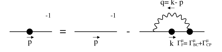
FIG. 1.: The inverse fermion propagator in quenched QED₄

Making use of the Feynman rules for this diagram leads to :

$$-{\it i}{\it S}_{F}^{-1}=-{\it i}{{\it S}_{F}^{0}}^{-1}-\int_{M}\frac{d^{4}k}{(2\,\pi)^{4}}\,(-{\it i}e\Gamma^{\mu}_{F})\,{\it i}S_{F}(k^{2})\,(-{\it i}e\gamma^{\nu})\,{\it i}\Delta_{\mu\nu}(q^{2})\quad,$$ (1)

where introducing several frequently used notations at once :

The Full Fermion Propagator is :

$$iS_{F}\equiv i\frac{F(p^{2})}{\not\!p-M(p^{2})}\equiv i\frac{Z(p^{2})}{\not\!p-M(p^{2})}\equiv i\frac{1}{A(p^{2})\,\not\!p-B(p^{2})}\quad,$$ (2)

and $F(p^{2})\equiv Z(p^{2})\equiv 1/A(p^{2})$ is the fermion wave-function renormalization, $M(p^{2})\equiv B(p^{2})/A(p^{2})\equiv Z(p^{2})B(p^{2})$ is the dynamical fermion mass.

The Full Photon Propagator is :

$$i\Delta_{\mu\nu}(p^{2})=-\frac{i}{p^{2}}\,\left[G(p^{2})\,\left(g_{\mu\nu}-\frac{p_{\mu}p_{\nu}}{p^{2}}\right)+\xi\frac{p_{\mu}p_{\nu}}{p^{2}}\right]\quad,$$ (3)

where $G(p^{2})\equiv 1/(1+\Pi(p^{2}))$ is the boson wave-function renormalization which is $1$ in the quenched approximation, and $\xi$ the covariant gauge parameter. We shall call $\left(g_{\mu\nu}-p_{\mu}p_{\nu}/p^{2}\right)$ the transverse part and $p_{\mu}\,p_{\nu}/p^{2}$ the longitudinal part. Finally, $\Gamma^{\mu}$ is the full fermion-boson vertex for which we use the CP ansatz, namely ($q\equiv k-p$)

$$\Gamma^{\mu}(k,p,q)=\Gamma_{\rm BC}^{\mu}(k,p)+\tau_{\rm CP}(k^{2},p^{2})\left[\gamma^{\mu}(p^{2}-k^{2})+(p+k)^{\mu}{\not\!q}\right]\>,$$ (4)

where $\Gamma_{\rm BC}$ is the usual Ball-Chiu part of the vertex which satisfies the Ward-Takahashi identity [12]

$$\Gamma^{\mu}_{\rm BC}(k,p) = \frac{1}{2}\left(\frac{1}{F(k^{2})}+\frac{1}{F(p^{2})}\right)\gamma^{\mu}$$ (5)

$$+ \frac{(k+p)^{\mu}}{k^{2}-p^{2}}\left\{\left(\frac{1}{F(k^{2})}-\frac{1}{F(p^{2})}\right)\frac{({\not\!k}+{\not\!p})}{2}-\left(\frac{M(k^{2})}{F(k^{2})}-\frac{M(p^{2})}{F(p^{2})}\right)\right\}\quad,$$ (6)

and the coefficient function $\tau_{6}$ is that chosen by Curtis and Pennington, i.e.,

$$\tau_{\rm CP}(k^{2},p^{2})=-\frac{1}{2\,d(k,p)}\left(\frac{1}{F(k^{2})}-\frac{1}{F(p^{2})}\right)\>,$$ (7)

where

$$d(k,p)=\frac{(k^{2}-p^{2})^{2}+[M^{2}(k^{2})+M^{2}(p^{2})]^{2}}{k^{2}+p^{2}}\>.$$ (8)

For studies of the nonperturbative renormalized fermion propagator, dynamical chiral symmetry breaking, and critical coupling $\alpha_{c}$ in quenched QED₄, it is necessary to choose a specific form for the fermion-photon proper vertex. While the exact form of this vertex is not known, there are constraints and symmetries which strongly restrict the allowable form. These include the Ward-Takahashi identity (WTI)[12]), the absence of artificial kinematic singularities, the requirements of multiplicative renormalizability (MR), and the need to agree with perturbation theory in the weak coupling limit. Furthermore, one should eventually ensure that the gauge dependence of the resulting fermion propagator is consistent with the Landau-Khalatnikov transformation [13] and that the value of the dynamical chiral symmetry breaking critical coupling ($\alpha_{c}$) should be gauge independent.

A number of discussions of the choice of the transverse part of the proper vertex can be found in the literature, e.g., Refs. [14, 15, 16, 17, 18, 19, 20, 21, 23]. We consider for our illustration here only the Curtis-Pennington (CP) vertex[15, 16, 17, 18, 24], which satisfies both the WTI and the constraints of multiplicative renormalizability. It is known that this vertex is not entirely adequate to ensure the gauge invariance of $\alpha_{c}$, although it is superior in this regard to the bare vertex for example[18, 24]. The choice of a vertex satisfying the WTI is a necessary but not sufficient condition to ensure the full gauge covariance of the Green’s functions of the theory and the gauge invariance of physical observables. Bashir and Pennington [20, 21] have proposed alternatives to the CP vertex, which ensure by construction that the critical coupling indeed becomes strictly gauge independent. All of the above studies were carried out with a UV cut-off regularization, where it was necessary to remove by hand an obvious explicit gauge-invariance violating term [19] which arose from the cut-off itself, (see for example Ref. [10] for a detailed discussion of this). We emphasize that the issue of interest here is not the construction of the ideal fermion-photon proper vertex, but rather to understand and remove explicit gauge-invariance violations arising from the UV cut-off regulator itself. For that purpose the CP vertex provides a useful illustrative example.

A Numerical Studies of the Fermion DSE

In quenched QED there is no renormalization of the electron charge and the appropriate photon propagator is just the bare one. The resulting nonlinear integral equation for the fermion propagator is solved numerically. The general features of dimensional regularization can be found in any recent textbook (e.g., Ref. [25]), and we use the notation $D=4-2\epsilon<4$ for the dimension of Euclidean space. Successive calculations with decreasing $\epsilon$ must be numerically extrapolated to $\epsilon=0$. For the UV cut-off regularization we simply cut-off the Euclidean four-dimensional loop integral at $\Lambda$ and verify that $\Lambda$ is sufficiently large. Clearly there is an ambiguity about exactly which loop momentum variable has the cut-off applied to it. In all calculations to date which use a UV cut-off a formal numerical extrapolation to $\Lambda\longrightarrow\infty$ has not been necessary.

The formalism is presented in Minkowski space and the Wick rotation into Euclidean space can then be performed once the equations to be solved have been written down. Although we use dimensional regularization, we cannot make use of the popular perturbative renormalization schemes such as $MS$ or $\overline{MS}$, since they cannot be applied in a nonperturbative context.

In the following equations and definitions, we will use $\epsilon$ to denote generic regularization dependence, where we must take the generic $\epsilon\to 0$ in the limit where the regularization is removed. For the UV cut-off case we understand $\epsilon\sim 1/\Lambda$. The renormalized inverse fermion propagator is defined through

$$S^{-1}_{R}(\mu;p)=\frac{1}{F_{R}(\mu;p^{2})}\not\!p-\frac{M_{R}(\mu;p^{2})}{F_{R}(\mu;p^{2})} = Z_{2}(\mu,\epsilon)[\not\!p-m_{0}(\epsilon)]-\Sigma_{0}(\mu,\epsilon;p)\quad,$$ (9)

$$= \not\!p-m(\mu)-{\Sigma}_{R}(\mu;p)\;\;\;,$$ (10)

where $\mu$ is the chosen renormalization scale, $m(\mu)$ is the value of the renormalized mass at $p^{2}=\mu^{2}$, $m_{0}(\epsilon)$ is the bare mass and $Z_{2}(\mu,\epsilon)$ is the wave-function renormalization constant. Due to the WTI for the fermion-photon proper vertex, we have for the vertex renormalization constant $Z_{1}(\mu,\epsilon)=Z_{2}(\mu,\epsilon)$. The renormalized and unrenormalized fermion self-energies are denoted as ${\Sigma}_{R}(\mu;p)$ and $\Sigma_{0}(\mu,\epsilon;p)$ respectively. These can be expressed in terms of Dirac and scalar pieces

$$\Sigma_{0}(\mu,\epsilon;p)=\Sigma^{d}_{0}(\mu,\epsilon;p^{2})\not\!p+\Sigma^{s}_{0}(\mu,\epsilon;p^{2})\;\;\;,$$ (11)

and similarly for ${\Sigma}_{R}(\mu;p)$. We do not explicitly indicate the dependence on $\epsilon$ of the renormalized quantities $1/F_{R}(\mu;p^{2})$, $M_{R}(\mu;p^{2})/F_{R}(\mu;p^{2})$ and ${\Sigma}_{R}(\mu;p)$, since for renormalized quantities we will always be interested in their $\epsilon\to 0$ limit. The renormalized mass function $M(p^{2})$ is renormalization point independent due to the nature of multiplicative renormalizability [10]. The renormalization point boundary condition

$$\left.S_{R}^{-1}(\mu;p)\right|_{p^{2}=\mu^{2}}=\not\!p-m(\mu)\quad,$$ (12)

implies that $F_{R}(\mu;\mu^{2})\equiv 1$ and $m(\mu)\equiv M(\mu^{2})$ and gives

$${\Sigma}^{d,s}_{R}(\mu;p^{2})=\Sigma_{0}^{d,s}(\mu,\epsilon;p^{2})-\Sigma_{0}^{d,s}(\mu,\epsilon;\mu^{2})\quad.$$ (13)

Also, the wave-function renormalization is given by

$$Z_{2}(\mu,\epsilon)=1+\Sigma_{0}^{d}(\mu,\epsilon;\mu^{2})\quad,$$ (14)

and for the bare mass $m_{0}(\epsilon)$

$$m_{0}(\epsilon)=\left[m(\mu)-\Sigma_{0}^{s}(\mu,\epsilon;\mu^{2})\right]/Z_{2}(\mu,\epsilon)\;\;\;.$$ (15)

Under a renormalization point transformation $\mu\to\mu^{\prime}$, $m(\mu^{\prime})=M({\mu^{\prime}}^{2})$ and $Z_{2}(\mu^{\prime},\epsilon)=Z_{2}(\mu,\epsilon)/F(\mu^{\prime};\mu^{2})$ as discussed in Ref. [10]. Since we are working here in the quenched approximation we have $Z_{3}(\mu,\epsilon)=1$, $e_{0}\equiv e(\mu)$, and the photon propagator ${\Delta}^{\mu\nu}(\mu;q)$ has its perturbative form where $G(p^{2})=1$.

The unrenormalized self-energy is given by the integral

$$\Sigma_{0}(\mu,\epsilon;p)=i\,(e(\mu)\nu^{\epsilon})^{2}\int\frac{d^{D}k}{(2\pi)^{D}}\gamma^{\lambda}{S}(\mu;k){\Gamma}^{\nu}(\mu;k,p){\Delta}_{\lambda\nu}(\mu;p-k)\>,$$ (16)

where $\nu$ is an arbitrary mass scale introduced in $D\equiv 4-2\epsilon$ dimensions so that the renormalized coupling $e(\mu)$ remains dimensionless in the dimensional regularization scheme. For the UV cut-off case we have no need of $\nu$ since $\epsilon=0$ but instead we integrate over a four-dimensional sphere whose radius is the UV cut-off $\Lambda$. The center of this sphere is often taken to be $k_{\mu}=0$, although one could equally well choose it to be at any location, e.g., at any $(k_{\mu}+c\,p_{\mu}+b_{\mu})=0$, where $c$ is an arbitrary real constant and $b_{\mu}$ is an arbitrary Euclidean four-momentum.

B Numerical Comparison

In Ref. [7], the renormalized dimensionally regularized fermion DSE for the Curtis-Pennington vertex in quenched approximation was studied numerically. Therein, it was noted that the fermion propagator extrapolated to $\epsilon=0$ using dimensional regularization differed from that obtained from using a cut-off regulator ‘as is’, but agreed with that obtained by using a cut-off regulator with the modification proposed by Ref. [19], within the numerical accuracy of the study. This was observed for a massive solution with the coupling $\alpha=1.5$ and the gauge parameter $\xi=0.25$. Here we explore whether this agreement holds at much increased numerical precision for the more numerically tractable case of $\alpha=0.6$ in a variety of gauges for both massive and massless solutions of the quenched fermion DSE.

1 Massive Case

Fig 4 shows a family of solutions calculated in dimensional regularization scheme with the regulator parameter $\epsilon$ decreased from 0.08 to 0.03 for the coupling $\alpha=0.6$. The gauge parameter is $\xi=0.25$, the renormalization point $\mu^{2}=10^{8}$ and the renormalized mass is $m(\mu)=400$. [Note that we have chosen our units such that $\mu^{2}=10^{8}$ and $m(\mu)=400$ in those units. We could equally well choose these units to be MeV, eV, GeV, etc. For a given solution we can simply multiply all mass scales in the problem by the same arbitrary constant and we still have a valid solution]. It is important to note the strong dependence of the solutions on $\epsilon$, even though this parameter is already rather small. The ultraviolet is most sensitive to this regulator, however even in the infrared there is considerable dependence due to the intrinsic coupling between these regions by the renormalization procedure. This strong dependence on $\epsilon$ should be contrasted with the situation in cut-off based studies where at rather modest cut-offs ($\Lambda^{2}\approx 10^{10}$) the renormalized functions $A$ and $M$ had already reached their asymptotic limits.

Also shown is the result of extrapolating these solutions to $\epsilon=0$ by fitting a polynominal quartic in $\epsilon$ at each momentum point. As was observed in [7], the linearity and stability of the extrapolation may be improved by a suitable choice of scale,$\nu$ : of the scales 1, 10, 100, 1000, and 10000, the latter two fit these criteria best. We show $\nu=10000$ on the graphs.

Fig. 5 shows this extrapolated solution along with the corresponding cut-off results, both with and without the aforementioned modification which eliminates a spurious term induced by the cut-off which breaks translational invariance. As may be clearly seen from the insert of Fig 5 the modified ultaviolet cut-off curve is indisguishable from the scaled dimensionally regularized one, while the naive cut-off curve clearly deviates from the others in the infrared. This observation is quantified by tables I and II which show absolute percentage comparisons of the finite renormalization and the mass function for the extrapolated solution with the modified and naive UV cut-off massive solutions respectively, with parameters as in Fig. 4 for two different scales and two different polynomial degrees. The agreement with the modified cut-off solution is seen to be excellent, and is three orders of magnitude better than the agreement with the naive cut-off.

Finally, Fig 6 shows a comparison in three different gauges, namely $\xi=0$, $\xi=0.25$ and $\xi=1$, of solutions of the fermion DSE extrapolated to $\epsilon=0$, and solutions using naive and modified UV cut-off regulators, with other parameters the same as in Fig. 4. The $A(p^{2})$ solutions are identical in Landau gauge, and the agreement between the extrapolated solution and the modified cut-off solution is readily distinguished in Feynman gauge. Owing to the approximate gauge invariance of the mass function, an insert is neccessary to reveal the same holds for $M(p^{2})$.

2 Massless Case

Fig 7 shows a family of solutions calculated in the dimensional regularization scheme with the regulator parameter $\epsilon$ from from 0.04 to 0.005 for the coupling $\alpha=0.6$, the gauge parameter $\xi=0.25$ and the renormalization point $\mu^{2}=10^{8}$. As in the massive case, there is a strong dependence of the renormalized function $A(p^{2})$ on the regulator $\epsilon$, although here the infrared is even more sensitive than the ultraviolet to $\epsilon$. This contrasts with cut-off solutions which reach their asymptotic limit at rather modest cut-offs.

Also shown is the result of extrapolating these solutions to $\epsilon=0$ by fitting a polynominal quartic in $\epsilon$ at each momentum point to $\log_{10}(A)$. This was appropriate because the the logarithmically scaled axes reveals the power-law character of the extrapolated solution.

In Fig 8 we show this extrapolated solution along with curves of the naive and modified cut-off solutions based on the power-behaved analytical formulae Eqs. (72) and (77) [15, 26, 27] discussed in the next section of the form

$$F(p^{2})=\left(p^{2}/\Lambda^{2}\right)^{\gamma}\,.$$ (17)

The curves are indistinguishable on the main figure: an insert reveals the extrapolated solution agrees with the modified cut-off solution. This is quantified by table III which shows absolute percentage comparisons of $A(p^{2})$ for these solutions. As in the massive case, the agreement with the modified cut-off solution is many orders of magnitude better than that with the naive cut-off.

Finally Fig 9 shows a comparison in three different gauges, namely $\xi=0$, $\xi=0.25$ and $\xi=1$, of solutions of the fermion DSE extrapolated to $\epsilon=0$, and solutions using naive and modified UV cut-off regulators, with other parameters the same as in Fig. 7. As in the massive case, the $A(p^{2})$ solutions are identical in Landau gauge, and the agreement between the extrapolated and modified cut-off solution is clear in Feynman gauge.

III Theoretical Studies on Translational Invariance of the DSE

The DSE approach to calculating any nonperturbative renormalized Green’s function in a renormalizable quantum field theory involves an integral over a loop momentum, where the integrand involves two or more renormalized nonperturbative Green functions[4]. If the Green’s function to be calculated from the loop integral corresponds to one of the primitively divergent diagrams, then regularization of the loop integration and renormalization will in general be necessary. The primitively divergent diagrams in QED are the 2 and 3-point Green functions, i.e., the fermion and photon propagators and the fermion-photon proper (i.e., one-particle irreducible) vertex. For other higher $n$-point Green’s functions the loop integrations in the DSE formalism are necessarily finite and renormalization of these quantities is not needed once the nonperturbative primitively divergent diagrams have been renormalized.

For instance the fermion self energy part of Eq. (1), as it stands, has a linear ultraviolet divergence because the integrand behaves like $\int\frac{d^{4}k}{k^{3}}$ for large $k$. Therefore, an ultraviolet regulator must be introduced in order to perform the loop integral. When the regulator is removed by renormalizing the theory, one should be left with a finite quantity which is independent of the scheme used. If two regularization schemes give different results then some symmetries have been violated by one (or both) of the regulators . The regulatization scheme should be chosen carefully so that gauge invariance and Poincare symmmetry in QED are preserved. For instance, while the Pauli Villars and dimensional regularization schemes respect gauge and translational invariance, UV cut-off regularization does not. However, one can attempt to use a UV cut-off regulator and still preserve these symmetries by imposing them on the regulator itself. Whether or not this procedure will be unique and conserve all symmetries is the key question. Here, a translationally invariant regularization scheme is defined to mean that the same results are obtained after arbitrary shifts in the definition of the loop mometum variable in the limit that the regularization is removed. Since a UV cut-off regularization is a restriction of the Euclidean loop-momentum integral to a four-dimensional hypersphere of radius $\Lambda$, we wish to ensure that in the limit $\Lambda\to\infty$ we find that the results are insensitive to the location of the centre of this hypersphere.

We are interested in establishing necessary and sufficient conditions for a UV cut-off regularization scheme to reproduce the results of a dimensional regularization scheme for the renormalized $n$-point Green’s functions. The scope of this present work is to establish a procedure for this for the electron self-energy. The procedures for removing unwanted contributions in a UV cut-off scheme are straightforward: (1) The best way to begin identifying such terms is to replace nonperturbative quantities in the integrand by their perturbative form; (2) Test that the resulting expression for the integral of the nonperturbative renormalized quantity is independent of the location of the hyperspheres center in the limit $\Lambda\to\infty$. Let us begin with an analysis of perturbation theory in order to understand the problem :

A Perturbation Theory as a Guide

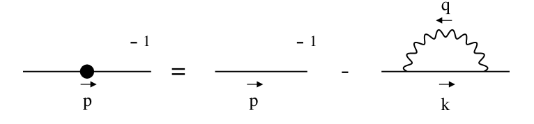
FIG. 2.: The inverse fermion propagator to one loop order in perturbation theory

Taking the weak coupling limit of Eq. (1) for massless QED₄ up to ${\cal{O}}(\alpha)$, substituting in the fermion and photon propagators and the 3-point vertex function, multiplying it by $\not\!p$ and taking its trace leads to the following expression :

$$\frac{1}{F(p^{2})}=1+\frac{i\,\alpha}{4\,\pi^{3}p^{2}}\,\int_{M}\frac{d^{4}k}{k^{2}q^{4}}\,\Big{\{}\left(-2\,k\cdot p\,q^{2}\right)+(\xi-1)\,\left(k^{2}\,p\cdot q-p^{2}\,k\cdot q\right)\Big{\}}\quad,\hskip 71.13188pt$$ (18)

$$= 1+\frac{i\,\alpha}{4\,\pi^{3}p^{2}}\,\int_{M}\frac{d^{4}k}{k^{2}q^{4}}\,\Big{\{}\underbrace{-3\,k\cdot p\,(k^{2}+p^{2})+4(k\cdot p)^{2}+2k^{2}p^{2}}+\xi\,\underbrace{\left(k^{2}\,p\cdot q-p^{2}\,k\cdot q\right)}\Big{\}}\quad.$$

$$\hskip 193.47882ptI_{T}\hskip 71.13188pt+\hskip 56.9055ptI_{L}\hskip 14.22636pt$$

where “M” denotes Minkowski space.

ANALYSIS:

(1) :

First we shall calculate the fermion wave-function renormalization within Dimensional Regularization, which respects the symmetries of QED. It is important to note that the first term and the coefficient of $(\xi-1)$ in the curly bracket of Eq. (18) give the same answer implying that the non-${\xi}$ part, $I_{T}$, of Eq. (LABEL:eq:perfermion2) vanishes and the ${\xi}$ part, $I_{L}$, yields the result as below :

$$\frac{1}{F(p^{2})}=1-\frac{\alpha\,\xi}{4\pi}\,\left[\frac{-1}{\epsilon}+\ln\left(\frac{p^{2}}{\nu^{2}}\right)-1+\gamma-\ln(4\,\pi)\right]\quad.$$ (20)

(2) :

Repeating the same calculation as above except this time using Cut-off Regularization we get with the hypersphere centre at $k_{\mu}=0$ :

$$\frac{1}{F(p^{2})}=1-\frac{\alpha\xi}{4\,\pi}\,\left(\ln\frac{p^{2}}{\Lambda^{2}}-\mbox{\framebox{ $\displaystyle{\bf\frac{1}{2}}$ }}\,\,\right)\quad.$$ (21)

Once again the integral of $I_{T}$ from Eq. (LABEL:eq:perfermion2) is zero.

The $1/2$ term in Eq. (21) is a consequence of cut-off regularization not preserving translational invariance and gauge covariance; in other words it is due to the non-conservation of current. The Landau-Khalatnikov (LK) transformations determines the gauge covariance of the theory in that if any Green’s functions of the theory are known in one gauge they are also known for any other gauge via this transformation. If in the Landau gauge, the fermion wave-function renormalization is $F(p^{2},\Lambda^{2})=\,A_{0}\,(p^{2}/\Lambda^{2})^{\gamma_{0}}$ then this transforms to the covariant gauge as $F(p^{2},\Lambda^{2})=\,A\,(p^{2}/\Lambda^{2})^{\gamma}$ where $\gamma=\,\gamma_{0}+\alpha\,\xi/4\pi$ and $A,A_{0}$ are constants,[27]. $\gamma_{0}$ is gauge independent term and in perturbation theory of ${\cal{O}}(\alpha^{2})$, [27]. Therefore, if one performs the perturbative expansion of $F(p^{2})=\,A\,(p^{2}/\Lambda^{2})^{\gamma}$ for small $\alpha$, then the $1/2$ term in Eq. (21) should be absent in order to ensure that the solution of the DSE for fermion wave-function renormalization is LK covariant.

As we shall see below this term can be removed by making use of the WTI or symmetry properties.

• 
  

• The WTI follows from gauge invariance. Applying it to the $\xi$-part of photon propagator in Eq. (1), separates out the term, $p\cdot q/q^{4}$, which is zero in any translational invariant scheme (odd in $q$). On the other hand, in cut-off regularization it is the source of the $1/2$ term in Eq. (21).

  
  
  
  

• To analyse the translational invariance  in cut-off regularization we shall shift the centre of the sphere from $k_{\mu}=0$ to $k_{\mu}=c\,p_{\mu}$, where $c$ is an arbitrary real constant, in Eq. (18) and Eq. (LABEL:eq:perfermion2). In so doing we obtain the following equations  :

  $$\int^{\Lambda}d^{4}k\,\frac{-2\,k\cdot p}{k^{2}\,(k-p)^{2}} = \pi^{2}p^{2}\left\{\ln\frac{p^{2}}{\Lambda^{2}}-\frac{1}{2}\right\}$$ (23)

  $$\hskip 28.45274pt\mathop{\longrightarrow}^{k\to k-cp}\qquad\pi^{2}p^{2}\left\{\ln\frac{p^{2}}{\Lambda^{2}}+\left(-\frac{1}{2}+c\right)+{\cal{O}}(\Lambda^{-1})\right\}\quad,$$

  $$\int^{\Lambda}d^{4}k\,\frac{-k\cdot q\,p^{2}}{k^{2}\,(k-p)^{4}} = \pi^{2}p^{2}\left\{\ln\frac{p^{2}}{\Lambda^{2}}\right\}$$ (25)

  $$\hskip 28.45274pt\mathop{\longrightarrow}^{k\to k-cp}\qquad\pi^{2}p^{2}\left\{\ln\frac{p^{2}}{\Lambda^{2}}+{\cal{O}}(\Lambda^{-1})\right\}\quad,$$

  $$\int^{\Lambda}d^{4}k\,\frac{p\cdot q}{(k-p)^{4}} = \pi^{2}p^{2}\left\{-\frac{1}{2}\right\}$$ (27)

  $$\hskip 28.45274pt\mathop{\longrightarrow}^{k\to k-cp}\qquad\pi^{2}p^{2}\left\{-\frac{(c+1)}{2}\right\}\quad,$$

  $$\int^{\Lambda}d^{4}k\,\frac{-3\,k\cdot p\,(k^{2}+p^{2})+4(k\cdot p)^{2}+2k^{2}p^{2}}{k^{2}\,(k-p)^{4}} = 0$$ (28)

  $$\mathop{\longrightarrow}^{k\to k-cp}\qquad \pi^{2}p^{2}\left\{\frac{3\,c}{2}+{\cal{O}}(\Lambda^{-1})\right\}\quad.$$ (29)

  Examination of Eqs. (23)- (29) reveals that with the exception of Eq. (25) (which is logarithmically divergent) all others are linearly divergent and VIOLATE translational invariance :

  Looking at the first term in $I_{L}$, which corresponds to Eq. (27), the WTI helps us to immediately recognize it as odd and linearly divergent. In cut-off regularization the position of the sphere is very important for the regularized quantities. If it is placed at $k_{\mu}=0$ then the $1/2$ term is generated in Eq. (21) and Eq. (27) which is consequence of the violation of translational invariance. On the other hand if the centre is located at $k_{\mu}=-p_{\mu}$ i.e. $c=-1$ then Eq. (27) is zero, translational invariance is preserved and cut-off is consistent with dimensional regularization.

  The second term in $I_{L}$ has only a logarithmic divergence and when it is shifted arbitrarily, the difference between the shifted and unshifted value vanishes as $\Lambda\longrightarrow\infty$ so this term is translational invariant even under cut-off regularization, Eq. (25).

  Finally we shall consider the transverse part, $I_{T}$ of Eq. (LABEL:eq:perfermion2) or Eq. (29). For large $k$ it becomes :

  $$I_{T} = \int d^{4}k\left\{-\frac{3\,k\cdot p}{k^{4}}+\frac{1}{k^{6}}\,\underbrace{\left(-4(k\cdot p)^{2}+k^{2}p^{2}\right)}\right\}\quad,$$ (31)

  $$\hskip 159.3356pt0$$

  as can be seen this expression, is zero (convergent) in any translationally invariant scheme. The reason for this is that the integral of the linearly divergent (also odd in $k$) term ($-3\,k\cdot p/k^{4}$) is zero and the logarithmically divergent second and third terms cancel each other out in any translationally invariant scheme, since they cancel after the angular integration about $k_{\mu}=0$. If Eq. (31) is centred at $k_{\mu}=0$ then even in cut-off regularization, the integral of the first term is identically zero. Conversely, if the hypersphere is centred at $k_{\mu}\neq 0$ the integral of the first term is non-zero. For instance, in Eq. (29), $k_{\mu}=c\,p_{\mu}$ will give $3\,c/2$. Hence, in order to be consistent with the translational invariant regularization $c$ must be ${\bf{zero}}$, i.e. when the transverse part is calculated one should keep the centre at $k_{\mu}=0$ or one must add suitable terms to compansate. Up until now, the general covariant gauge case has been discussed. However, often it is easier to calculate the fermion wave-function renormalization in a specific gauge. Take for example Feynman gauge, $\xi=1$, in this case Eq. (18) greatly simplifies and we are left with only the first term of the integral, Eq. (23). From this equation we can see that in order to be consistent with the arbitrary covariant gauge calculation and dimensional regularization calculation $c$ can conveniently be chosen to be $1/2$. In the arbitrary covariant gauge calculation, the non-$\xi$ part of the integral in Eq. (18) is given by Eqs. (23-25-27). In this case, the terms violating translational invariance cancel out in Eq. (23) and Eq. (27) if and only if $c=0$. In the Feynman gauge no cancellation occurs so that the term violating the translational invariance in Eq. (23) must vanish identically. This can only be done if the hypersphere is centred at $k_{\mu}=p_{\mu}/2$, namely $c=1/2$. We emphasize that we can equally well choose either centre for any gauge. The two choices described here give the same translationally invariant result since the two choices can be seen to differ by just the right term (that vanishes in a translationally invariant scheme).

  To summarize: In an arbitrary covariant gauge $I_{T}$ vanishes as it should, if the centre of the hypersphere is located at $k_{\mu}=0$. In that case, centering the cut-off integration for $I_{L}$ at $k_{\mu}=q_{\mu}$ gives the result consistent with the translationally invariant dimensional regularization. This is one convenient procedure. In the specific case of the Feynman gauge this same translationally invariant result can also, for example, be conveniently obtained by centering the hypersphere of the entire integrand at $k_{\mu}=p_{\mu}/2$. These two ways of proceeding, of course, lead to the same expression for the total integral in Feynman gauge as they should.

(3)  Renormalization :

(a) : Applying multiplicative renormalization (MR) requires the following relations between renormalized, $F_{R}$, and unrenormalized, $F_{0}$, fermion wave-function renormalization :

$$F_{R}=Z_{2}^{-1}\,F_{0}\quad,$$ (32)

where $Z_{2}$ denotes the fermion renormalization constant. If we apply MR to the perturbation theory order by order, then the unrenormalized fermion wave-function renormalization which is calculated in an uncorrected cut-off scheme up to order ${\alpha}$ is :

$$F_{0}(p^{2},\Lambda^{2}) = 1+\frac{\alpha\,\xi}{4\,\pi}\left(\ln\frac{p^{2}}{\Lambda^{2}}-\frac{1}{2}\right)+{\cal{O(\alpha^{2})}}\quad,$$ (33)

and the fermion renormalization constant is :

$$Z_{2}(\mu^{2},\Lambda^{2})=1+\frac{\alpha\,\xi}{4\,\pi}\left(\ln\frac{\mu^{2}}{\Lambda^{2}}-\frac{1}{2}\right)+{\cal{O}}(\alpha^{2})$$ (34)

One can renormalize $F_{0}$ by choosing $F_{R}(p^{2},\mu^{2})=1$ at ${p^{2}=\mu^{2}}$ and find the renormalized wave-function renormalization from Eq. (32) as :

$$F_{R}(p^{2},\mu^{2})=1+\frac{\alpha\,\xi}{4\,\pi}\ln\frac{p^{2}}{\mu^{2}}+{\cal{O}}(\alpha^{2})\quad,$$ (35)

which can be summed to all orders as :

$$F_{R}(p^{2})=\left(\frac{p^{2}}{\mu^{2}}\right)^{\frac{\alpha\,\xi}{4\,\pi}}\quad.$$ (36)

(b) : Applying subtractive renormalization to the dimensional regularization calculation, Eq. (20), we get :

$${F_{R}(p^{2})} = 1+\Sigma_{R}(p^{2};\mu^{2})$$ (37)

$$= 1+\left(\Sigma_{0}(p^{2};\mu^{2},\Lambda^{2})-\Sigma_{0}(\mu^{2};\mu^{2},\Lambda^{2})\right)$$ (38)

$$= 1+\frac{\alpha\xi}{4\,\pi}\ln\frac{p^{2}}{\mu^{2}}+{\cal{O}}(\alpha^{2})$$ (39)

$$= \left(\frac{p^{2}}{\mu^{2}}\right)^{\frac{\alpha\xi}{4\pi}}\quad,$$ (40)

where $\Sigma_{R}(p^{2};\mu^{2})$ is renormalized fermion self energy. As we see, even if we start with the incorrect unrenormalized fermion wave-function renormalization, we get the same renormalized results for both cut-off and dimensional regularization schemes in perturbation theory. This is because the WTI is taken care of automatically in perturbation theory; however this is not the case in nonperturbative theory. So, starting with the wrong quantity, gives the wrong answer in nonperturbative theory. If one does not impose translational invariance on the regulator as a necessary condition then the result will be different in cut-off and dimensional regularization schemes.

Since the violation of translational invariance in a naive UV cut-off scheme appears to be the only source of gauge-covariance violation, the restoration of translational invariance should also remove any explicit source of gauge-covariance violation. Translational invariance is certainly a necessary condition, but one should ask whether it is a sufficient condition. At present we know of no rigorous mathematical argument that proves such a sufficiency. All that can be said is that it is difficult to conceive of integrands where this would not be the case. Indeed, field theories which yield different behaviors from dimensional regularization and translationally invariant UV cut-off approaches would need to be specified by both a Lagrangian density and by a particular choice of regularization scheme.

We now move on to nonperturbative QED and investigate how much information from perturbation theory we can make use of. Let us start with Ball-Chiu (BC) plus Curtis-Pennington (CP) vertex in massless QED₄.

B Prescription for Consistency with Dimensional Regularization

Thus far we have seen how translational invariance is violated in the UV cut-off regularization and have described what must be done to obtain the same result as dimensional regularization for the fermion self-energy in quenched QED₄. In this section we shall formulate a more general prescription.

In any translationally invariant regularization scheme the following expression is true:

translationally (41)

invariant   scheme (42)

$$I(p^{2})=\int d^{4}k\,I(k,p,\theta) = \int d^{4}k\,I(k^{\prime},p,\theta)\quad,$$ (43)

where the integrand $I(k,p,\theta)$ is related to the shifted integrand $I(k^{\prime},p,\theta)$ through $k^{\prime}_{\mu}=k_{\mu}+c\,p_{\mu}+b_{\mu}$. Unfortunately, in cut-off regularization the above equality is not true for renormalized integrands in the limit $\Lambda\longrightarrow\infty$ unless the integrand, $I(k,p,\theta)$, is at worst logarithmically divergent, i.e., in general

$${\mathop{\lim}_{\Lambda\rightarrow\infty}}\left(\int^{\Lambda}d^{4}k\,I(k,p,\theta)-\int^{\Lambda}d^{4}k\,I(k^{\prime},p,\theta)\right)\neq 0\quad.$$ (45)

Since in the limit $\Lambda\to\infty$ the renormalized Green functions (and their various component parts) are necessarily finite, the contribution from the integrands must be vanishingly small at infinity. This ensures that the result of the integral is independent of whether the shape of the integral region was hyperspherical, hypercubic or any other shape one might construct. In other words, once translational invariance in the UV cut-off approach has been ensured and the limit $\Lambda\to\infty$ has been taken, the resulting renormalized nonperturbative quantities are entirely independent of the details of how the limit was taken. To ensure the above equality we need to develop an appropriate, unique, translationally invariant cut-off regularization scheme. This can be summarized by the following prescription :

1. Start with the integral $\int^{\Lambda}d^{4}k\,I(k,p,\theta)$.

2. Choose any centre for the four-dimensional hypersphere with radius $\Lambda$.

3. Add $\int d^{4}k\,\Delta I_{i}$ terms which would vanish in any translational invariant regularization scheme to eliminate the defect of all linearly divergent terms in perturbation theory, where

   $$\int d^{4}k\,\Delta I_{i}=\int d^{4}k\,\left[I_{i}(k^{\prime},p,\theta)-I_{i}(k,p,\theta)\right]=\,0\quad.$$ (46)

   and where $I_{i}(k,p,\theta)$ is some integrand. The above difference is zero in dimensional regularization but will introduce an artificial term which contributes to the next to leading order terms in a cut-off scheme. The number of $\Delta I_{i}$ terms needed is related to the number of linearly divergent terms in the integrand ,

   $$\int^{\Lambda}d^{4}k\,I^{\prime}(k,p,\theta)=\int^{\Lambda}d^{4}k\,\left[I(k,p,\theta)+\sum_{i}\,d_{i}\,\Delta I_{i}(k,k^{\prime},p,\theta)\right]\quad.$$ (47)

   where $d_{i}$ are constants.

4. The $d_{i}$’s are to be fixed by equating Eq. (47) with the translational invariant results (dimensional regularization results) from perturbation theory.

C Application of the Prescription

Let us consider the fermion wave-function renormalization, $F(p^{2})$, in perturbation theory as an example. As we shall disscuss later one can see the residue of the violated symmetries in the cut-off scheme in the nonperturbative case even after renormalization. Of course this is not the case in perturbation theory. Therefore, since in this section we deal with the perturbative expansion of the fermion wave-function renormalization, we shall use regularized quantities in order to pin down the terms which cause problems in the nonperturbative case.

The integrand in Eq. (LABEL:eq:perfermion2) can be divided into three parts :

$$I(k,p,\theta)=I_{0}(k,p,\theta)+\,\xi\left[I{{}^{\rm odd}}(k,p,\theta)+\,I{{}^{\rm trans.}}(k,p,\theta)\right]\quad,$$ (48)

where

$$\left.\begin{array}[]{cll}\displaystyle I\,_{0}(k,p,\theta)&\equiv&\displaystyle\frac{\left(-3\,k\cdot p\,(k^{2}+p^{2})+4(k\cdot p)^{2}+2k^{2}p^{2}\right)}{k^{2}\,q^{4}}\quad,\\ \displaystyle I\,{{}^{\rm odd}}(k,p,\theta)&\equiv&\displaystyle\frac{k^{2}\,p\cdot q}{k^{2}\,q^{4}}\quad,\\ \displaystyle I\,{{}^{\rm trans.}}(k,p,\theta)&\equiv&\displaystyle\frac{-p^{2}\,k\cdot q}{k^{2}\,q^{4}}\quad,\end{array}\,\,\,\right\}$$ (52)

where $I^{{\rm odd}}$ is odd in $q$ and $I^{{\rm trans}}$ is a translationally invariant integrand (since it is only logarithmically divergent).

Let us apply the prescription to the ${\xi}$ part in Eq. (48) first :

1. Start with,

   $$I_{\xi}(p)\equiv\int^{\Lambda}d^{4}k\left[I\,{{}^{\rm odd}}(k,p,\theta)+\,I\,{{}^{\rm trans.}}(k,p,\theta)\right]\quad.$$ (53)

2. Choose $k_{\mu}$ as the centre of the hypersphere $\Lambda$.

3. Add $\int d^{4}k\,\Delta I_{i}$ terms :

   $$I^{\prime}\,_{\xi}(p) = \int^{\Lambda}d^{4}k\left[I^{\prime}\,{{}^{\rm odd}}(k,p,\theta)+\,I^{\prime}\,{{}^{\rm trans.}}(k,p,\theta)\right]\quad,$$ (54)

   $$= \int^{\Lambda}d^{4}k\,\Big{\{}\,\,\,I{{}^{\rm odd}}(k,p,\theta)+d_{1}\,\left[I{{}^{\rm odd}}(k^{\prime},p,\theta)-I{{}^{\rm odd}}(k,p,\theta)\right]$$ (56)

   $$+\hskip 36.98866ptI{{}^{\rm trans}}(k,p,\theta)+d_{2}\,\left[I{{}^{\rm trans}}(k^{\prime},p,\theta)-I{{}^{\rm trans}}(k,p,\theta)\right]\Big{\}}\quad,$$

   where $k^{\prime}$ is the shifted $k$, in general $k^{\prime}_{\mu}=k_{\mu}+cp_{\mu}+b_{\mu}$.

4. Fix $d_{1}$ by using the following :

• In any translational invariant scheme, any odd part of the integral should be zero :

  $$\int d^{4}kI^{\prime}\,{{}^{\rm odd}}(k,p)=\int d^{4}kI^{\prime}\,{{}^{\rm odd}}(k^{\prime},p)=0$$ (57)

  Therefore the odd part of Eq. (56) can be written as :

  $$I^{{}^{\prime}\rm odd}(p)\,=\,0=\,\int^{\Lambda}d^{4}k\,\left\{(1-d_{1})\,I{{}^{\rm odd}}(k,p,\theta)+d_{1}\,I{{}^{\rm odd}}(k^{\prime},p,\theta)\right\}\quad.$$ (58)

  For instance, if we locate the centre of the sphere at $k_{\mu}=0$ and then we shift the loop momentum to $k_{\mu}\longrightarrow k_{\mu}+p_{\mu}$ then :

  $$\int^{\Lambda}d^{4}k\,I{{}^{\rm odd}}(k,p,\theta) = -\frac{1}{2}\quad,$$ (59)

  $$\int^{\Lambda}d^{4}k\,I{{}^{\rm odd}}(k+p,p,\theta) = \int^{\Lambda}d^{4}k\,\frac{(p\cdot k)}{k^{4}}=0\quad.$$ (60)

  Hence, in order to satisfy Eq. (58),

  $$d_{1}=1$$

• The $I^{\rm trans}$ part is independent of shifts in $k$, i.e. it is translationally invariant since it is only logarithmically divergent :

  $$I^{{}^{\prime}\rm trans}(p)=\int^{\Lambda}\,I{{}^{trans}}(k,p,\theta)\quad=\int^{\Lambda}\,I{{}^{trans}}(k^{\prime},p,\theta)\quad\mbox{independent of $d_{2}$}$$ (61)

  Now let us consider the $I_{0}$ part of Eq. (48) :

• We know from dimensional regularization that in perturbation theory $\int d^{4}k\,I_{0}(k,p,\theta)=0$  .

  $$I_{0}^{\prime}(p)=\,0=\,\int^{\Lambda}d^{4}k\left\{(1-d_{3})\,I_{0}(k,p,\theta)+d_{3}\,I_{0}(k^{\prime},p,\theta)\right\}\quad.$$ (62)

  Within cut-off regularization :

  $$\int^{\Lambda}d^{4}k\,I_{0}(k,p,\theta) = 0\quad,$$ (63)

  $$\int^{\Lambda}d^{4}k\,I_{0}(k^{\prime},p,\theta) = -\frac{3}{2}\quad,$$ (64)

  where again here the first integral is centred at $k_{\mu}=0$ and the second integral at $k_{\mu}=p_{\mu}$. So, for Eq. (62) to be true

  $$d_{3} = 0\quad.$$

The above prescription for the cut-off regularization scheme should ensure the same result as the dimensional regularization scheme.

D Massless, Quenched QED₄ with CP-Vertex

FIG. 3.: Quenched Dyson-Schwinger Equation with Curtis-Pennington Vertex

Inserting the full fermion and bare photon propagators and full fermion-photon vertex (BC+CP) into Eq. (1), then multiplying the result by $\not\!p$, and taking its trace we get :

$$\frac{1}{F(p^{2})} = 1+\frac{i\,\alpha}{8\,\pi^{3}p^{2}}\,\int_{M}\frac{d^{4}k}{k^{2}q^{4}}\,\times$$

$$\Bigg{\{}\left(1+\frac{F(k^{2})}{F(p^{2})}\right)\,\Bigg{[}\hskip 51.21495pt\left(-3\,k\cdot p\,(k^{2}+p^{2})+4(k\cdot p)^{2}+2k^{2}p^{2}\right)+\xi\,\left(k^{2}\,p\cdot q-p^{2}\,k\cdot q\right)\Bigg{]}$$

$$+\left(1-\frac{F(k^{2})}{F(p^{2})}\right)\,\Bigg{[}\frac{(k^{2}+p^{2})}{(k^{2}-p^{2})}\,\left(-3\,k\cdot p\,(k^{2}+p^{2})+4(k\cdot p)^{2}+2k^{2}p^{2}\right)+\xi\,\left(k^{2}\,p\cdot q+p^{2}\,k\cdot q\right)\Bigg{]}\Bigg{\}}\,.$$

After moving from Minkowski space to Euclidean space by performing a Wick rotation, we can carry out the above integrals. By looking at Eq. (LABEL:eq:bccp), we notice that the fermion wave-function, $F(p^{2})$, is the only nonperturbative quantity and does not depend on the angle between $k$ and $p$. At the level of calculating angular integrals, everything is the same as for the perturbation theory case, hence we know how to deal with these integrals. As we have seen before, the first term of the integral in Eq. (LABEL:eq:bccp), earlier called $I_{T}$, is zero,( Eq. (29)). So then we have:

$$\frac{1}{F(p^{2},\Lambda^{2})}=1-\frac{\alpha\,\xi}{4\,\pi^{3}}\,\int_{E}\,\frac{d^{4}k}{k^{2}\,q^{4}}\,\left(k^{2}\,p\cdot q-p^{2}k\cdot q\,\frac{F(k^{2},\Lambda^{2})}{F(p^{2},\Lambda^{2})}\right)\,.$$ (66)

The above equation can be expressed in terms of renormalized quantities as :

$$\frac{1}{Z_{2}(\mu^{2},\Lambda^{2})\,F_{R}(p^{2},\mu^{2})}=1-\frac{\alpha\,\xi}{4\,\pi^{3}\,p^{2}}\,\int_{E}\,\frac{d^{4}k}{k^{2}\,q^{4}}\,\left(k^{2}\,p\cdot q-p^{2}k\cdot q\,\frac{F_{R}(k^{2},\mu^{2})}{F_{R}(p^{2},\mu^{2})}\right)\quad.$$ (67)

Multiplying this equation by $F_{R}(p^{2},\mu^{2})$ to leave the fermion renormalization constant, $Z_{2}$, alone on the left hand side and performing some of the integrals, we find :

$$\frac{1}{Z_{2}(\mu^{2},\Lambda^{2})}=F_{R}(p^{2},\mu^{2})+\frac{\alpha\,\xi}{4\,\pi}\,\int_{0}^{\Lambda^{2}}\,dk^{2}\,\left(\frac{k^{2}}{p^{4}}\,F_{R}(p^{2},\mu^{2})\,\theta(p^{2}-k^{2})+\frac{1}{k^{2}}\,F_{R}(k^{2},\mu^{2})\,\theta(k^{2}-p^{2})\right)\quad.$$

If we write the same expression for $p^{2}=\mu^{2}$ and subtract it from Eq. (LABEL:eq:peqmu), we get :

$$0=F_{R}(p^{2},\mu^{2})-F_{R}(\mu^{2},\mu^{2})+\,\frac{\alpha\,\xi}{4\,\pi}\,\Bigg{\{}\frac{1}{2}\,F_{R}(p^{2},\mu^{2})\,-\,\frac{1}{2}\,F_{R}(\mu^{2},\mu^{2})+\int_{p^{2}}^{\mu^{2}}\,\frac{dk^{2}}{k^{2}}\,F_{R}(k^{2},\mu^{2})\Bigg{\}}\quad.$$

Considering that the fermion wave-function renormalization $F(p^{2})$ must obey the power behaviour $F_{R}(p^{2},\mu^{2})=(p^{2}/\mu^{2})^{\nu}$ in the nonperturbative massless case, then after carrying out the radial integral Eq. (LABEL:eq:differ) can be written as:

$$F_{R}(p^{2},\mu^{2})-F_{R}(\mu^{2},\mu^{2})=-\frac{\alpha\,\xi}{4\,\pi}\,\Bigg{\{}\left(\frac{1}{2}-\frac{1}{\nu}\right)\,\left[F_{R}(p^{2},\mu^{2})-\,F_{R}(\mu^{2},\mu^{2})\right]\Bigg{\}}\quad.$$ (70)

Comparing both sides of Eq. (70) we find that[24],[27]

$$\nu=\frac{2\alpha\xi}{\alpha\xi+8\pi}\quad$$ (71)

giving the solution

$$F_{R}(p^{2}/\mu^{2}) = \left(\frac{p^{2}}{\mu^{2}}\right)^{2\alpha\xi/(\alpha\xi+8\pi)}.$$ (72)

Unlike perturbation theory, the third and fourth terms of Eq. (LABEL:eq:differ) do not cancel each other, so that the first term, $1/2$, on the right hand side of Eq. (70) survives. We have seen in perturbation theory that keeping $\int d^{4}k\,p\cdot q/q^{4}$ which is the source of this term did not make any difference in the renormalized quantities, because in perturbation theory it is :

$$\int d^{4}k\,\frac{p\cdot q}{q^{4}}-\int d^{4}k\,\frac{\mu\cdot q^{\prime}}{q^{\prime 4}}=\,0\quad,$$ (73)

where $q^{\prime}=k-\mu$. BUT it does make a difference in nonperturbative studies. Assuming the transverse vertex vanishes in the Landau gauge means that $\nu=\alpha\,\xi/4\,\pi$, i.e. $F_{R}(p^{2},\mu^{2})=(p^{2}/\mu^{2})^{{\alpha\,\xi}/{4\,\pi}}$, from the LKF transformation. Eq. (71) is different from $\alpha\,\xi/4\,\pi$ due to the fact that translational invariance is broken by cut-off regularization. Therefore, one must cancel the $\int d^{4}k\,p\cdot q/q^{4}$ term in Eq. (66) in order to recover the correct behaviour of the fermion wave-function renormalization. Removing this term from Eq. (66), we find :

$$\frac{1}{F(p^{2},\Lambda^{2})}=1+\frac{\alpha\,\xi}{4\,\pi^{3}}\,\int_{E}\,\frac{d^{4}k}{k^{2}\,q^{4}}\,\left(p^{2}k\cdot q\,\frac{F(k^{2},\Lambda^{2})}{F(p^{2},\Lambda^{2})}\right)\quad,$$ (75)

so that

$$\nu = \frac{\alpha\,\xi}{4\,\pi}\quad$$ (76)

giving the solution of this equation as

$$F_{R}(p^{2}/\mu^{2}) = \left(\frac{p^{2}}{\mu^{2}}\right)^{\alpha\,\xi/4\,\pi}.$$ (77)

This is exactly the same as the result obtained from a nonperturbative dimensional regularization scheme [19]. As a result of the above discussions we see that the modified cut-off prescription can be succesfully applied to massless quenched QED. Therefore, after applying the prescription for this case one can see the agreement between dimensional regularization and the modified cut-off result numerically in Figs.8 and 9.

E Massive, Quenched QED₄ with CP-Vertex

The fermion wave-function renormalization for the massive QED₄ case using BC and CP vertices can be written as :

$$\frac{1}{F(p^{2})} = 1+\frac{i\,\alpha}{8\,\pi^{3}p^{2}}\,\int_{M}\frac{d^{4}k}{\left(k^{2}-M^{2}(k^{2})\right)\,q^{4}}\,\times$$ (82)

$$\Bigg{\{}\left(1+\frac{F(k^{2})}{F(p^{2})}\right)\,\Bigg{[}\hskip 51.21495pt\left(-3\,k\cdot p\,\left(k^{2}+p^{2}\right)+4(k\cdot p)^{2}+2k^{2}p^{2}\right)+\xi\,\left(k^{2}\,p\cdot q-p^{2}\,k\cdot q\right)\Bigg{]}$$

$$+\left(1-\frac{F(k^{2})}{F(p^{2})}\right)\,\Bigg{[}\frac{1}{\left(k^{2}-p^{2}\right)}\,\,\,\frac{\left(-3\,k\cdot p\,\left(k^{2}+p^{2}\right)+4(k\cdot p)^{2}+2k^{2}p^{2}\right)}{d}+\xi\,\left(k^{2}\,p\cdot q+p^{2}\,k\cdot q\right)\Bigg{]}$$

$$-\left(1-\frac{F(k^{2})}{F(p^{2})}\right)\,\Bigg{[}\frac{1}{\left(k^{2}-p^{2}\right)}\,\frac{2\,\Delta^{2}\,\left(M^{2}(k^{2})+M^{2}(p^{2})\right)^{2}}{d}\Bigg{]}$$

$$+\left(M^{2}(k^{2})-M(k^{2})M(p^{2})\frac{F(k^{2})}{F(p^{2})}\right)\,\frac{1}{(k^{2}-p^{2})}\,\Bigg{(}-4\Delta^{2}+\xi\,(k^{2}-p^{2})^{2}p\cdot q\Bigg{)}\Bigg{\}}\quad,$$

where

$$d = \frac{(k^{2}-p^{2})^{2}+[M^{2}(k^{2})+M^{2}(p^{2})]^{2}}{k^{2}+p^{2}}\quad,$$

$$\Delta^{2} = (k\cdot p)^{2}-k^{2}p^{2}\quad.$$

In this case, the second and third lines of Eq. (82) are exactly the same as in the massless case except for the mass term in the denominator. Hence, for calculating these lines, the only difference between the massless and massive cases will come from radial integrals and the presence of a mass term in the denominator only makes the calculation convergent more quickly. So we do not encounter any worse than a logarithmic divergence. The third and fourth lines of Eq. (82) will introduce new terms which depend on the mass function but the integrals do not have any worse divergence than the logarithmic divergence because for large momenta the mass function behaves like $M(k^{2})\,\alpha\,k^{-\gamma},0<\gamma<2$, [24], [9],[10]. Therefore, there is no danger of violating translational invariance.

Of course, in the massive case with the Curtis-Pennington or the real transverse vertex, the fermion wave-function renormalization will not give $1$ in Landau gauge. In other words, the transversality condition [28], [23] is not applicable for these vertices. As a result of that, for such vertices, we can not use the condition $F(p^{2})=1$ in Landau gauge in the prescription. Consequently, the third item, Eq. (62), in the prescription must be changed to :

$$I_{0}^{\prime}(p)={\overline{f(p)}} = \int^{\Lambda}d^{4}k\,I^{\prime}_{0}(k,p,\theta)=\int^{\Lambda}d^{4}k\,I^{\prime}_{0}(k^{\prime},p,\theta)$$ (83)

$$= \int^{\Lambda}d^{4}k\left\{(1-d_{3})\,I_{0}(k,p,\theta)+d_{3}\,I_{0}(k^{\prime},p,\theta)\right\}$$ (84)

$$= (1-d_{3})\,f(p)+d_{3}\,f^{\prime}(p)\quad.$$ (85)

Knowing that $k_{\mu}=0$ is the right centre for $I_{0}$ term in massless QED and required to satisfy the massless limit when $M(p^{2})\longrightarrow 0$, we should also choose the centre at $k_{\mu}=0$ for the massive case. This means ${\overline{f(p)}}=f(p)$, then Eq. (85) becomes :

$$0=d_{3}\,\left[f^{\prime}(p)-f(p)\right]\quad,$$ (86)

Due to the fact that [$f^{\prime}(p)\neq f(p)$], $d_{3}$ should be :

$$d_{3}=0\quad.$$ (87)

This is just the prescription used in the modified UV cut-off scheme which we have already seen gives such excellent numerical agreement with the dimensional regularization studies.

IV Conclusions and Outlook

Studying Quantum Electrodynamics necessarily introduces divergences. We have seen explicitly that the violation of translational invariance in nonperturbative studies using an ultraviolet cut-off leaves an error in the renormalized result. Hence, if one wants to use cut-off regularization and find the translationally invariant answer for the calculated renormalized quantity then a modification is needed. Since the nonperturbative quantity must give the perturbative result in the weak coupling limit, it is simplest to attempt to identify these modifications within perturbation theory. Once this is done we can attempt to generalise it to the nonperturbative case. Fortunately, in the case of the fermion self-energy calculation one can establish a nonperturbative framework on top of the perturbative one.

In this work the violation of translational invariance for the electron self-energy is analyzed in detail and a prescription is presented in order to calculate the quantity without breaking translational invariance in cut-off regularization. More precisely we mean that violations of translational invariance are no worse than logarithmic and so for the subtracted (i.e., renormalized) integral in the limit $\Lambda\,\longrightarrow\,\infty$, translational invariance is restored. In this regard, the electron self-energy is used a test case and as a result we have seen that a suitably modified cut-off scheme and the dimensional regularization scheme should be in agreement. Careful numerical studies (see Tables I–III and Figs. 5–6 and  8–9) have demonstrated this agreement to high precision. In closing we note that while we can always add terms with arbitrary coefficients which would vanish in a translationally invariant regularization scheme, our approach will only be useful when there are sufficient known constraints to determine these coefficients uniquely. We are currently attemping to extend this approach to include the photon self energy, so that we can study unquenched QED₄ using a translationally invariant ultraviolet cut-off regularization scheme.

TABLE I.: Absolute percentage comparison of finite renormalization $A(p^{2})$ for $\epsilon\to 0$ with modified and naive UV cut-off massive solutions, with parameters as in Fig. 4. Here $\nu$ represents the scale of the extrapolated solutions, while ‘degree’ is the degree of the polynomial used to fit the extrapolated solution at each point. Higher degree polynomials show no variation from the quintic.

$\nu$	degree	cutoff	$p^{2}=10^{-6}$	$p^{2}=10^{-2}$	$p^{2}=10^{2}$	$p^{2}=10^{6}$	$p^{2}=10^{10}$	$p^{2}=10^{14}$
1000	4	mod	$2.8\times 10^{-5}$	$2.8\times 10^{-5}$	$2.9\times 10^{-5}$	$2.2\times 10^{-5}$	$2.3\times 10^{-5}$	$4.7\times 10^{-5}$
		naive	$3.7\times 10^{-2}$	$3.7\times 10^{-2}$	$3.7\times 10^{-2}$	$3.2\times 10^{-2}$	$3.3\times 10^{-2}$	$9.8\times 10^{-2}$
1000	5	mod	$2.8\times 10^{-5}$	$2.8\times 10^{-5}$	$2.8\times 10^{-5}$	$2.2\times 10^{-5}$	$2.2\times 10^{-5}$	$5.8\times 10^{-5}$
		naive	$3.7\times 10^{-2}$	$3.7\times 10^{-2}$	$3.7\times 10^{-2}$	$3.2\times 10^{-2}$	$3.3\times 10^{-2}$	$9.8\times 10^{-2}$
10000	4	mod	$2.6\times 10^{-5}$	$2.6\times 10^{-5}$	$2.8\times 10^{-5}$	$2.9\times 10^{-5}$	$1.2\times 10^{-5}$	$1.5\times 10^{-5}$
		naive	$3.7\times 10^{-2}$	$3.7\times 10^{-2}$	$3.7\times 10^{-2}$	$3.2\times 10^{-2}$	$3.3\times 10^{-2}$	$9.8\times 10^{-2}$
10000	5	mod	$2.5\times 10^{-5}$	$2.5\times 10^{-5}$	$2.8\times 10^{-5}$	$3.0\times 10^{-5}$	$1.2\times 10^{-5}$	$1.8\times 10^{-5}$
		naive	$3.7\times 10^{-2}$	$3.7\times 10^{-2}$	$3.7\times 10^{-2}$	$3.2\times 10^{-2}$	$3.3\times 10^{-2}$	$9.8\times 10^{-2}$

TABLE II.: Absolute percentage comparison as above, but for the mass function $M(p^{2})$.

$\nu$	degree	cutoff	$p^{2}=10^{-6}$	$p^{2}=10^{-2}$	$p^{2}=10^{2}$	$p^{2}=10^{6}$	$p^{2}=10^{10}$	$p^{2}=10^{14}$
1000	4	mod	$0.00012$	$0.00012$	$0.00012$	$0.00013$	$0.00026$	$0.055$
		naive	$0.33$	$0.33$	$0.33$	$0.33$	$0.63$	$1.9$
1000	5	mod	$0.00012$	$0.00012$	$0.00012$	$0.00013$	$0.00026$	$0.054$
		naive	$0.33$	$0.33$	$0.33$	$0.33$	$0.63$	$1.9$
10000	4	mod	$0.00026$	$0.00026$	$0.00026$	$0.00046$	$0.00049$	$0.035$
		naive	$0.33$	$0.33$	$0.33$	$0.32$	$0.63$	$2.0$
10000	5	mod	$0.00026$	$0.00026$	$0.00026$	$0.00046$	$0.00047$	$0.035$
		naive	$0.33$	$0.33$	$0.33$	$0.32$	$0.63$	$2.0$

TABLE III.: Absolute percentage comparison of the finite renormalization $A(p^{2})$ for $\epsilon\to 0$ with modified and naive UV cut-off massless solutions, with parameters as in Fig. 7. Here ‘degree’ is the degree of the polynomial used to fit the extrapolated solution at each point. Higher degree polynomials show no variation from the quintic.

degree	cutoff	$p^{2}=10^{-10}$	$p^{2}=10^{-5}$	$p^{2}=10^{0}$	$p^{2}=10^{5}$	$p^{2}=10^{10}$	$p^{2}=10^{15}$	$p^{2}=10^{20}$
4	mod	$6.9\times 10^{-5}$	$6.2\times 10^{-6}$	$2.1\times 10^{-6}$	$5.3\times 10^{-7}$	$7.3\times 10^{-6}$	$1.4\times 10^{-4}$	$8.4\times 10^{-4}$
	naive	$2.9\times 10^{-1}$	$2.1\times 10^{-1}$	$1.3\times 10^{-1}$	$4.9\times 10^{-2}$	$3.3\times 10^{-2}$	$1.1\times 10^{-1}$	$1.9\times 10^{-1}$
5	mod	$6.8\times 10^{-5}$	$6.1\times 10^{-6}$	$2.1\times 10^{-6}$	$5.8\times 10^{-7}$	$7.5\times 10^{-6}$	$1.4\times 10^{-4}$	$8.5\times 10^{-4}$
	naive	$2.9\times 10^{-1}$	$2.1\times 10^{-1}$	$1.3\times 10^{-1}$	$4.9\times 10^{-2}$	$3.3\times 10^{-2}$	$1.1\times 10^{-1}$	$1.9\times 10^{-1}$

FIG. 4.: The finite renormalization $A(p^{2})$ and mass function $M(p^{2})$ of massive solutions of the fermion DSE for various choices of the regulator parameter $\epsilon$, with coupling $\alpha=0.6$, gauge parameter $\xi=0.25$, renormalization point $\mu^{2}=10^{8}$, renormalized mass $m(\mu)=400$ and scale $\nu=1$. Also shown are $A(p^{2})$ and $M(p^{2})$ extrapolated to $\epsilon=0$, obtained by fitting polynomials quartic in $\epsilon$ at each momentum point.

FIG. 5.: The finite renormalization $A(p^{2})$ and mass function $M(p^{2})$ of the massive solution of the fermion DSE extrapolated to $\epsilon=0$ from Fig. 4, compared with solutions using naive and modified UV cut-off regulators. Note that the curves are almost indistinguishable on the main figure: the inserts in the figure for the infra-red reveal the excellent agreement between the extrapolated (quartic fit) dimensional regularization solutions and the modified cut-off solutions which lie on top of each other.

FIG. 6.: A comparison in three different gauges of the finite renormalization $A(p^{2})$ and mass function $M(p^{2})$ of the massive solution of the fermion DSE extrapolated to $\epsilon=0$, and solutions using naive and modified UV cut-off regulators. Other parameters are the same as in Fig. 4. As in the massless case, the $A(p^{2})$ solutions are identical in Landau gauge. The agreement between the extrapolated (quartic) dimensional regularization solution and the modified cut-off solution is readily seen in the Feynman gauge and the curves again lie on top of each other in all gauges. The naive cut-off solution clearly disagrees with dimensional regularization result. Owing to the approximate gauge invariance of the mass function, an insert is neccessary to reveal that the same holds for $M(p^{2})$.

FIG. 7.: The finite renormalization $A(p^{2})$ of chirally symmetric zero-mass solutions of the fermion DSE for various choices of the regulator parameter $\epsilon$, with coupling $\alpha=0.6$, gauge parameter $\xi=0.25$, renormalization point $\mu^{2}=10^{8}$ and scale $\nu=1$. Also shown is $A(p^{2})$ extrapolated to $\epsilon=0$, obtained by fitting a polynomial quartic in $\epsilon$ to $\log_{10}(A)$ at each point. The logarithmically scaled axes reveals the power-law character of the extrapolated solution (straight line is this figure). The invariance in $\epsilon$ of the point at $p^{2}\approx 10^{-4}$ is only approximate, the spread being about 5 parts in $10^{3}$.

FIG. 8.: The finite renormalization $A(p^{2})$ of the chirally symmetric zero-mass solution of the fermion DSE extrapolated to $\epsilon=0$ from Fig. 7, compared with the formulae (72) and (77) for the naive and modified UV cut-off solutions respectively. The curves are indistinguishable on the main figure: an insert reveals the extrapolated solution agrees with the modified cut-off solution.

FIG. 9.: A comparison in three different gauges of the finite renormalization $A(p^{2})$ of the chirally symmetric zero-mass solution extrapolated to $\epsilon=0$ and the naive and modified UV cut-off solutions given by eqns. (72) and (77) respectively. Other parameters are the same as in Fig. 7. The curves are identical in Landau gauge: in Feynman gauge, the agreement between the extrapolated and modified UV cut-off solutions is clearly visible.